computational fluid dynamics analysis of jets with ...lyrintzi/aiaa-2005-2887-loren.pdfcomputational...

Computational Fluid Dynamics Analysis of Jets with

Internal Forced Mixers

L. A. Garrison∗ A. S. Lyrintzis† G. A. Blaisdell‡

Purdue University, West Lafayette, IN, 47907, USA

W. N. Dalton§

Rolls-Royce Corporation, Indianapolis, IN, 41234, USA

In the current study Computational Fluid Dynamics (CFD) analysis using the Reynoldsaveraged Navier-Stokes (RANS) equations with the two-equation Shear Stress Transport(SST) turbulence model is performed for internally mixed jets with the goal of accuratelypredicting the development of the turbulence in the resulting jet plumes. The CFD resultsfrom an axisymmetric and three forced mixer test cases are compared to experimentalParticle Image Velocimetry (PIV) data. The CFD results of the mean velocities in the jetplume compare well with experimental PIV data with the exception of a slightly slowercenterline velocity decay rate. In addition, the CFD results of the turbulence levels in thejet shear layer take longer to spread to the centerline. The CFD results also show an over-prediction in the turbulence levels in the initial portion of the jet shear layer. However,the peak turbulence levels in the CFD results further downstream in the jet plumes forthe forced mixer test cases are in agreement with PIV data. In addition, the CFD resultsfrom this study support the hypothesis that the additional noise source seen at high Machnumbers (high Mach number lift - HML) in the high frequency range of the acoustic datafor these mixers at near critical pressure ratios is due to the interaction of the turbulentstreamwise vorticies shed by the mixers and a normal shock at the final nozzle exit.

Nomeclature

Roman Symbols SubscriptsU Jet velocity c Core flow propertyD Jet diameter b Bypass flow propertyH Lobe penetration height m Fully mixed jet propertyM Mach number f Flight stream propertyk Turbulence kinetic energy 1 Flow property upstream of a shockp Static pressure 2 Flow property downstream of a shockL11 Longitudinal turbulence length scalea Constant (Ribner) AbbreviationsK1 Non-dimensional wave number NPR Nozzle Pressure Ratiof Frequency HML High Mach number LiftA Area CFD Computational Fluid Dynamics

RANS Reynolds Averaged Navier-StokesGreek Symbols PIV Particle Image Velocimetryλ Velocity ratioω Specific turbulence dissipation rate

∗Graduate Research Assistant, School of Aeronautics and Astronautics, Student Member AIAA.†Professor, School of Aeronautics and Astronautics, Associate Fellow AIAA.‡Associate Professor, School of Aeronautics and Astronautics, Senior Member AIAA.§Manager Mechnaical Methods and Acoustics, Member AIAA.

1 of 20

American Institute of Aeronautics and Astronautics

I. Introduction

The prediction of the jet noise from complex configurations continues to be a problem for industry despiteover a half century of research in flow generated noise. The lack of accurate noise prediction methods

for the complex geometries applicable to modern jet engines prevents engine companies from factoring noiseinto the design of new mixer geometries. As a result, engine companies are forced to design, build, andperform relatively expensive experimental tests of new nozzle and mixer designs to determine whether theywill meet FAA noise requirements.

One recent approach to modeling the noise for the complex configuration of a jet with an internal forcedmixer has been developed which uses modified single jet noise spectra to build a noise prediction.1,2 Thistwo-source noise prediction method, which is a modification of the four-source method for predicting coaxialjets,3,4 uses a combination of two single jet predictions which are filtered and shifted by empirically derivedsource strength terms. This type of noise model, with two empirically determined parameters, has beenpreviously shown to be capable of accurately matching experimental noise data for a family of 12-lobe forcedmixers.

The goal of the current research effort is to replace the empirically derived two-source noise modelparameters with model parameters that are determined from CFD analysis, ultimately resulting in a stand-alone noise prediction tool. In this paper, the CFD analyses of the various mixer geometries are validatedagainst experimental PIV data. In this study, CFD analyses of a confluent (axisymmetric) and three forcedmixer geometries are performed to determine the turbulence quantities in the jet plumes. The mean flowand turbulence data from the CFD solutions are compared to experimental Particle Image Velocimetry(PIV) data of the jet plume flow fields. In addition, the CFD results from this study are shown to supportthe hypothesis for the origin of the high Mach number lift (HML) phenomenon, which is seen in the highfrequency region of the acoustic data for these mixers at set points with near critical pressure ratios.5 Itis shown that only the cases that exhibit the HML phenomenon have a normal shock at the nozzle exit,supporting the theory that the HML noise source is due to the interaction of the turbulent streamwisevorticies shed by the forced mixers and a normal shock at the final nozzle exit.

II. Experimental Data

The experimental Particle Image Velocimetry (PIV) data for the mixers evaluated in this study wastaken in Aeroacoustic Propulsion Laboratory at NASA Glenn.6 PIV measurements were taken at twelveplanes perpendicular to the jet axis at locations ranging from 0.1 to 10 diameters downstream of the finalnozzle exit. The stereo PIV arrangement used in the experimental test program measured all three velocitycomponents. Both mean and rms velocities are available. The PIV data was corrected to align the jetcenterline axis with the origin of PIV reference frame. The PIV data was then interpolated onto a uniformpolar grid to aide in further post-processing.

The results for one confluent mixer and three forced mixer geometries are presented in this paper. Theconfluent mixer geometry, shown in Figure 1, is an axisymmetric splitter plate which separates the bypassand core flows. All three forced mixers, which are essentially convoluted splitter plates, have 12 lobes andare of similar designs. An example of a forced mixer geometry is shown in Figure 2. The primary differencebetween the three forced mixers is the amount of lobe penetration, H, defined as the difference between themaximum and minimum radii at the end of the splitter plate as shown in Figure 3. The values of the lobepenetration heights non-dimensionalized by the final nozzle exit diameter, D, are given in Table 1 for thethree forced mixers. In addition to the four mixer geometries, three nozzle geometries are also evaluated.These nozzle geometries are the baseline L0 nozzle, the L1 nozzle (75% of the baseline length), and the L2nozzle (50% of the baseline length). The profiles for the three nozzle geometries are shown in Figure 4.

In this study, flow field results are presented for a total of three operating set points. The primary andsecondary nozzle pressure ratios, the velocity ratios, and the flight Mach numbers for these set points areshown in Table 2. The confluent mixer CFD results are compared to the PIV data at set points 312 and5000. The nozzle pressure ratios of the core and bypass flows are equal in set point 5000 which simulates asingle jet. Forced mixer CFD results are compared to PIV data for set points 112 and 312.

2 of 20


Table 1. Forced mixer properties.

Mixer ID H/D Description12CL 0.199 12 Lobe, Low Penetration12UM 0.241 12 Lobe, Medium Penetration12UH 0.280 12 Lobe, High Penetration

Table 2. Experimental data test conditions.

Set Point NPRc NPRb λ Mf

112 1.39 1.44 0.68 0.2312 1.74 1.82 0.62 0.25000 1.44 1.44 1.00 0.0

III. CFD Analysis

An initial study of the axisymmetric confluent mixer case was performed using both FLUENT7 and theWIND code,8 which solves the Reynolds averaged Navier-Stokes (RANS) equations. In this initial studythe performance of a number of two-equation turbulence models was assessed. It was ultimately determinedthat the two-equation Shear Stress Transport (SST) turbulence model9 yielded the best agreement with thePIV data. All of the CFD analyses of the steady-state jet plume flow fields presented in this paper werecalculated using the WIND code with the two-equation SST turbulence model. The boundary conditions arecalculated based on the total pressure, total temperature, mass flow rate, and ambient conditions recordedduring the PIV tests. In addition, the inflow boundary conditions for the turbulence kinetic energy, k, aredetermined based on the turbulence levels in the first plane of the PIV data. The inflow boundary conditionsfor the specific turbulence dissipation rate, ω, are determined based on the turbulence kinetic energy andthe assumption that the turbulent viscosity is 100 times the molecular viscosity. It was seen that varyingthe inflow turbulence viscosity ratio over several orders of magnitude had a relatively small impact on theturbulence levels in the jet plume.

A. Confluent Mixer

The axisymmetric grid used for the confluent mixer calculations contains approximately 80,000 grid points.A refined grid with twice as many points in the axial and radial directions was also tested. The turbulencelevels in the jet plume of the fine grid were almost identical to those with the 80,000 point grid. Thecomputational domain of the jet plume extends out 5.5 diameters in the radial direction and 10 diametersdownstream of the nozzle exit. The axisymmetric calculations, run on 6 processors of a Linux cluster, take1.5 seconds per cycle. Typically 8,000 cycles are run to obtain a converged solution, resulting in a turnaround time of approximately 3.5 hours.

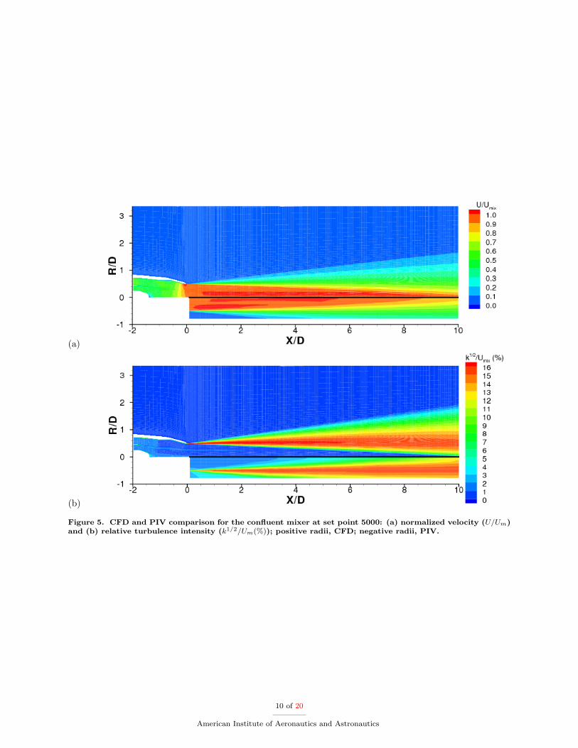
The CFD results for the confluent mixer with the baseline L0 nozzle at set point 5000 (simulated single jet)are compared to the experimental PIV data in Figure 5. Contours of the non-dimensional mean streamwisevelocity (U/Um) and relative turbulence intensity (k1/2/Um) are shown for the CFD solution (positive radii)and PIV data (negative radii) in Figure 5. From the comparison of the mean velocity it is seen that the CFDresults slightly under-predict the decay of the centerline velocity. The comparison of the turbulence kineticenergy shows a slight over-prediction in the CFD turbulence kinetic energy in the jet shear layer region upto 6 diameters downstream of the nozzle exit. In addition the turbulence in the PIV data spreads to thecenterline much faster than in the CFD results.

The CFD results for the confluent mixer with the baseline L0 nozzle at set point 312 are compared tothe experimental PIV data in Figure 6. From the comparison of the mean streamwise velocity it is seenthat once again the CFD slightly under-predicts the decay of the centerline velocity. The comparison ofthe turbulence kinetic energy shows a consistent over-prediction of the turbulence in the CFD results. Inaddition, it is once again seen that the turbulence in the PIV data spreads to the centerline much faster

3 of 20


than what is predicted by CFD.

B. Forced Mixers

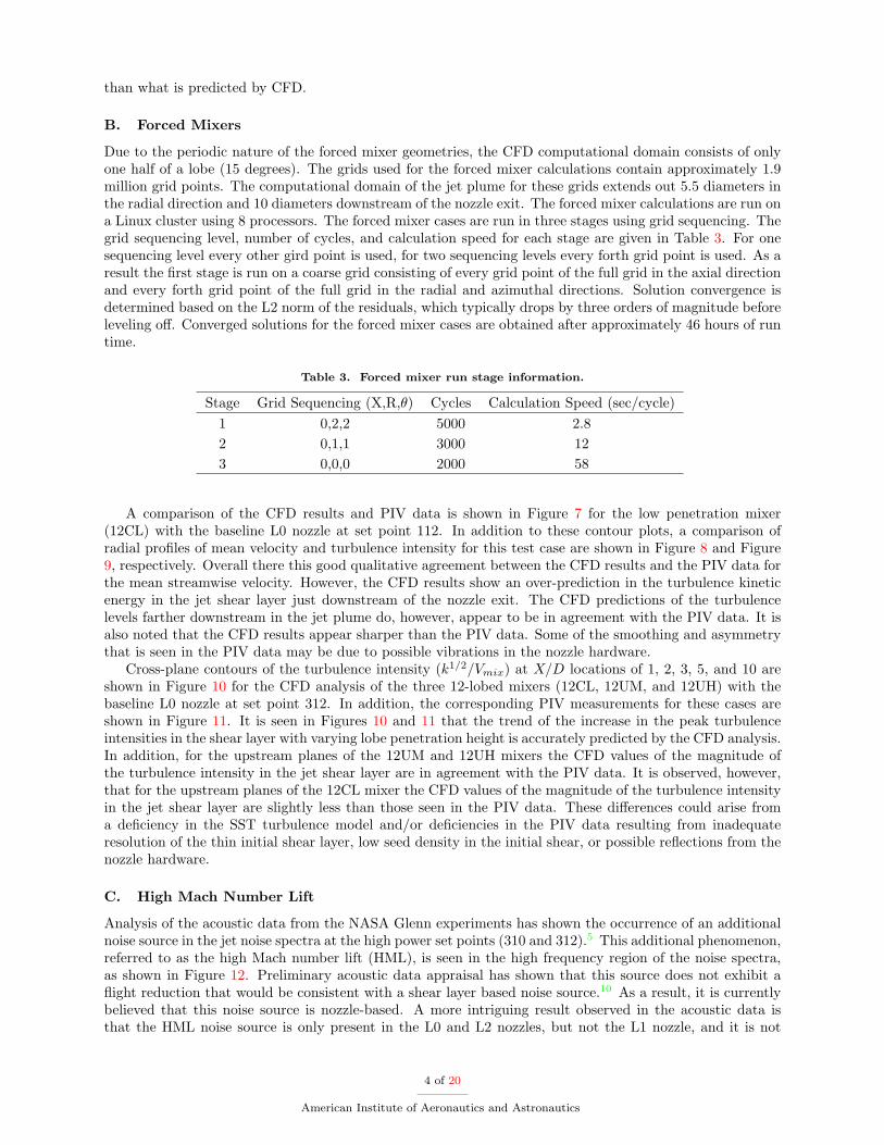
Due to the periodic nature of the forced mixer geometries, the CFD computational domain consists of onlyone half of a lobe (15 degrees). The grids used for the forced mixer calculations contain approximately 1.9million grid points. The computational domain of the jet plume for these grids extends out 5.5 diameters inthe radial direction and 10 diameters downstream of the nozzle exit. The forced mixer calculations are run ona Linux cluster using 8 processors. The forced mixer cases are run in three stages using grid sequencing. Thegrid sequencing level, number of cycles, and calculation speed for each stage are given in Table 3. For onesequencing level every other gird point is used, for two sequencing levels every forth grid point is used. As aresult the first stage is run on a coarse grid consisting of every grid point of the full grid in the axial directionand every forth grid point of the full grid in the radial and azimuthal directions. Solution convergence isdetermined based on the L2 norm of the residuals, which typically drops by three orders of magnitude beforeleveling off. Converged solutions for the forced mixer cases are obtained after approximately 46 hours of runtime.

Table 3. Forced mixer run stage information.

Stage Grid Sequencing (X,R,θ) Cycles Calculation Speed (sec/cycle)1 0,2,2 5000 2.82 0,1,1 3000 123 0,0,0 2000 58

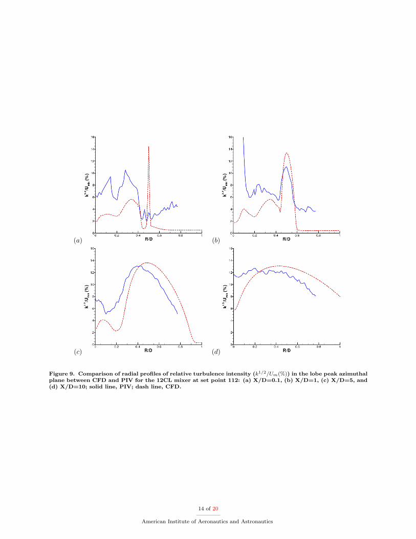
A comparison of the CFD results and PIV data is shown in Figure 7 for the low penetration mixer(12CL) with the baseline L0 nozzle at set point 112. In addition to these contour plots, a comparison ofradial profiles of mean velocity and turbulence intensity for this test case are shown in Figure 8 and Figure9, respectively. Overall there this good qualitative agreement between the CFD results and the PIV data forthe mean streamwise velocity. However, the CFD results show an over-prediction in the turbulence kineticenergy in the jet shear layer just downstream of the nozzle exit. The CFD predictions of the turbulencelevels farther downstream in the jet plume do, however, appear to be in agreement with the PIV data. It isalso noted that the CFD results appear sharper than the PIV data. Some of the smoothing and asymmetrythat is seen in the PIV data may be due to possible vibrations in the nozzle hardware.

Cross-plane contours of the turbulence intensity (k1/2/Vmix) at X/D locations of 1, 2, 3, 5, and 10 areshown in Figure 10 for the CFD analysis of the three 12-lobed mixers (12CL, 12UM, and 12UH) with thebaseline L0 nozzle at set point 312. In addition, the corresponding PIV measurements for these cases areshown in Figure 11. It is seen in Figures 10 and 11 that the trend of the increase in the peak turbulenceintensities in the shear layer with varying lobe penetration height is accurately predicted by the CFD analysis.In addition, for the upstream planes of the 12UM and 12UH mixers the CFD values of the magnitude ofthe turbulence intensity in the jet shear layer are in agreement with the PIV data. It is observed, however,that for the upstream planes of the 12CL mixer the CFD values of the magnitude of the turbulence intensityin the jet shear layer are slightly less than those seen in the PIV data. These differences could arise froma deficiency in the SST turbulence model and/or deficiencies in the PIV data resulting from inadequateresolution of the thin initial shear layer, low seed density in the initial shear, or possible reflections from thenozzle hardware.

C. High Mach Number Lift

Analysis of the acoustic data from the NASA Glenn experiments has shown the occurrence of an additionalnoise source in the jet noise spectra at the high power set points (310 and 312).5 This additional phenomenon,referred to as the high Mach number lift (HML), is seen in the high frequency region of the noise spectra,as shown in Figure 12. Preliminary acoustic data appraisal has shown that this source does not exhibit aflight reduction that would be consistent with a shear layer based noise source.10 As a result, it is currentlybelieved that this noise source is nozzle-based. A more intriguing result observed in the acoustic data isthat the HML noise source is only present in the L0 and L2 nozzles, but not the L1 nozzle, and it is not

4 of 20


present for the confluent mixer geometry. It has been shown by previous CFD work that for the BaselineL0 nozzle geometry a small region of supersonic flow occurs near the nozzle exit (close to the nozzle wall),terminating in a normal shock.11 It has therefore been hypothesized that the HML noise source could becaused by turbulence from the streamwise vorticies generated by the forced mixer passing through a normalshock at the nozzle exit.

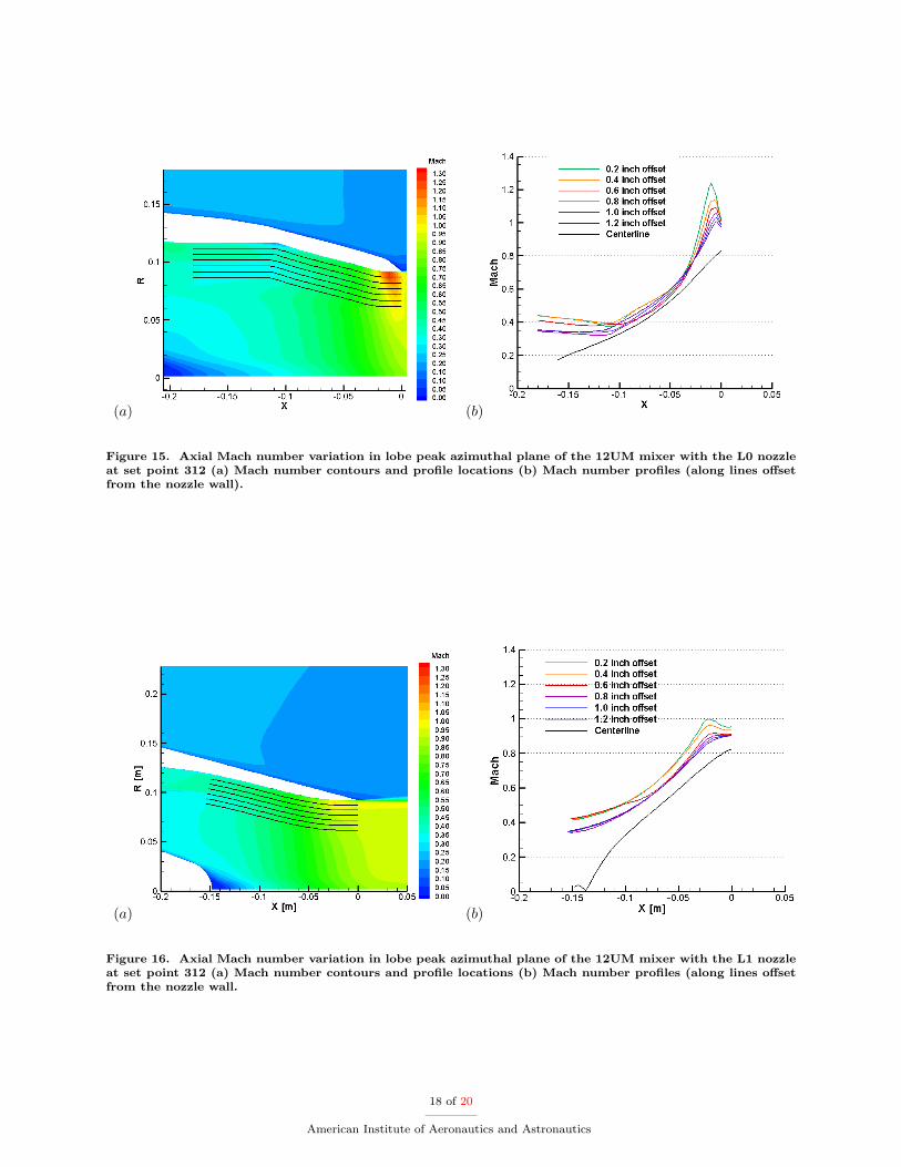
Supersonic flow could occur in a convergent nozzle at sub-critical pressure ratios as a result of flow turningeffects. The axial variation of the angle between the interior nozzle wall and the jet axis, which illustratesthe flow turning effects of the various nozzles, is shown in Figure 13 for the L0, L1, and L2 nozzles. It is seenin Figure 13 that the L0 and L2 nozzles have a relatively rapid transition from the convergent section of thenozzle to the parallel section at the nozzle exit. In contrast, the L1 nozzle has a more gradual transition.The CFD results in the lobe peak azimuthal plane of the 12UM mixer at set point 312 with the L0, L1, andL2 nozzles are shown in Figure 14. From these results it is seen that both the L0 and L2 nozzle geometriesproduce a normal shock at the final nozzle exit. However, a shock is not present at the nozzle exit for the L1nozzle geometry. These findings are consistent with the flow turning effects shown in Figure 13. In addition,the Mach number profiles along lines offset from the nozzle wall are shown in Figures 15 and 16 for the L0and L1 nozzles, respectively.

The turbulence kinetic energy just upstream of the normal shock for the 12-lobed mixers with the L0nozzle is shown in Figure 17 for set point 312. In this figure the bold contour lines correspond to thesupersonic region and the thin contour lines correspond to the subsonic flow region. An initial attemptto quantify the strength of HML noise source resulting from the turbulence-shock interaction is made byapplying the CFD data to the theoretical work of Ribner.12,13,14 The non-dimensional HML source strengthis estimated as

HML ∝∫A

k

U2m

(p2 − p1

p2

)0.323

e−3.5p2−p1

p2 dA

where p2 − p1 is the difference in static pressure across the shock and the area of integration is the shocksurface. The HML source strength is proportional to the turbulence kinetic energy, as suggested by Ribner.The functional dependence of the HML source strength with the shock strength (static pressure rise) wasdetermined based on a curve fit to the Ribner theory. The calculated HML source strength values are plottedon the shock surface for the three 12-lobed mixers in Figure 18. The total integrated HML source strengthfor the 12UM mixer is 1.99 times stronger than the total HML source strength for the 12CL mixer, which isconsistent with the acoustic experimental data.10

In addition to the source strength, the HML noise source peak frequencies are estimated using the Ribnertheory.14 The peak frequency is estimated as

f =K1UA

2πaL11

where UA is the velocity upstream of the shock, a is a constant (1.339), L11 is the longitudinal turbulencelength scale, and K1 is the peak wave number of the far-field noise one-dimensional power spectra, which isestimated as 0.75 from the Ribner results. The upstream velocity and longitudinal turbulence length scalesare calculated using the CFD data. The HML noise source peak frequencies for the 12CL mixer at setpoint 310 are shown in Figure 19. It is seen that these estimated peak frequencies are consistent with thefrequency range of the HML noise source as seen in Figure 12. The far-field directivity of the HML noisesource has also been estimated by combining the Ribner theory for the refracted noise emission angle alongwith a geometric acoustics shear layer refraction correction. The results of this analysis are compared tothe difference between Sound Pressure Level spectra of the L0 nozzle and L1 nozzle cases at 20 kHz for the12CL mixer at set point 310 in Figure 20, where the far-field angle is referenced from the jet axis. It is seenin Figure 20 that these estimates of the far-field directivity of the HML noise source are in agreement withthe experimental acoustic data.

IV. Conclusion

In this study CFD analyses of internally mixed jets are performed. The jet plume flow fields resultingfrom one axisymmetric and three forced mixer geometries are considered. For the axisymmetric confluentmixer cases the mean streamwise velocity values are in qualitative agreement with the PIV results. The

5 of 20


largest differences in the CFD predictions for these cases are the over-prediction of the turbulence kineticenergy in the shear layer and the slight under-prediction of the centerline velocity decay rate. For the threedimensional forced mixer cases the CFD predicted mean streamwise velocity and a turbulence kinetic energyvalues are in agreement with the PIV results, with the exception of an over-prediction of turbulence kineticenergy in the jet shear layer just downstream of the nozzle exit. The turbulence levels farther downstreamfor the various forced mixers were in agreement with the experimental PIV data. The final step in creatinga stand-alone noise prediction methodology is the formalization of the process in which the two-source noisemodel parameters are determined from the CFD results. Finally, the results from the CFD analysis of the12UM mixer with the various nozzle geometries supports the present theory that the origin of the high Machnumber lift noise source, which is seen in the high frequency range of the acoustic data at near criticalpressure ratios, is due to the interaction of turbulence with a normal shock at the nozzle exit.

Acknowledgments

This work has been funded by the Aeroacoustics Research Consortium (AARC) as part of a collaborativeproject with Dr. Brian Tester and Dr. Mike Fisher at the Institute of Sound and Vibration Research (ISVR),University of Southampton, UK. The first author is also supported by a Purdue Research Fellowship. AllWIND calculations were performed on the School of Aeronautics and Astronautics 104-processor LINUXcluster acquired by a Defense University Research Instrumentation Program (DURIP) grant sponsored byARO. The experimental PIV data used in this study has been provided by Dr. James Bridges at the NASAGlenn Research Center.

References

1Garrison, L. A., Dalton, W. N., Lyrintzis, A. S., and Blaisdell, G. A., “Semi-Empirical Noise Models for Predicting theNoise from Jets with Forced Mixers,” AIAA Paper No. 2004-2898, May 2004.

2Tester, B. J., Fisher, M. J., and Dalton, W. N., “A Contribution to the Understanding and Prediction of Jet NoiseDeneration in Forced Mixers,” AIAA Paper No. 2004-2897, May 2004.

3Fisher, M. J., Preston, G. A., and Bryce, W. D., “A Modelling of the Noise from Simple Coaxial Jets Part I: WithUnheated Primary Flow,” Journal of Sound and Vibration, Vol. 209, No. 3, 1998, pp. 385–403.

4Fisher, M. J., Preston, G. A., and Mead, C. J., “A Modelling of the Noise from Simple Coaxial Jets Part II: With HeatedPrimary Flow,” Journal of Sound and Vibration, Vol. 209, No. 3, 1998, pp. 405–417.

5Tester, B. J. and Fisher, M. J., “21st Century Jet Noise Test Data Appraisal,” ISVR Consultancy Ref:6920-Final Report,November 2003.

6Bridges, J. and Wernet, M. P., “Cross-Stream PIV Measurements of Jets with Internal Lobed Mixers,” AIAA Paper No.2004-2896, May 2004.

7“FLUENT 6.0 User’s Guide,” Fluent Inc., 2001.8“WIND v5.0 User’s Guide,” NPARC Alliance, NASA Glenn Research Center and USAF Arnold Engineering Development

Center, 2004.9Menter, F., “Two-Equation Eddy-Viscosity Turbulence Models for Engineering Applications,” AIAA Journal , Vol. 32,

No. 3, 1994, pp. 1598–1605.10Tester, B. J. and Fisher, M. J., “Jet Noise Generation by Forced Mixers: Part II Flight Effects,” AIAA Paper No.

2005-3094, May 2005.11Wright, C. W., Investigating Correlations Between Reynolds Averaged Flow Fields and Noise for Forced Mixed Jets,

Master’s thesis, School of Aeronautics and Astronautics, Purdue University, West Lafayette, IN, May 2004.12Ribner, H. S., “Convection of a Pattern of Vorticity Through a Shock Wave,” NACA TR-1164, 1954.13Ribner, H. S., “Shock-Turbulence Interaction and the Generation of Noise,” NACA TR-1233, 1955.14Ribner, H. S., “Spectra of Noise and Amplified Turbulence Emanating from Shock-Turbulence Interaction,” AIAA Jour-

nal , Vol. 25, No. 3, 1986, pp. 436–442.

6 of 20


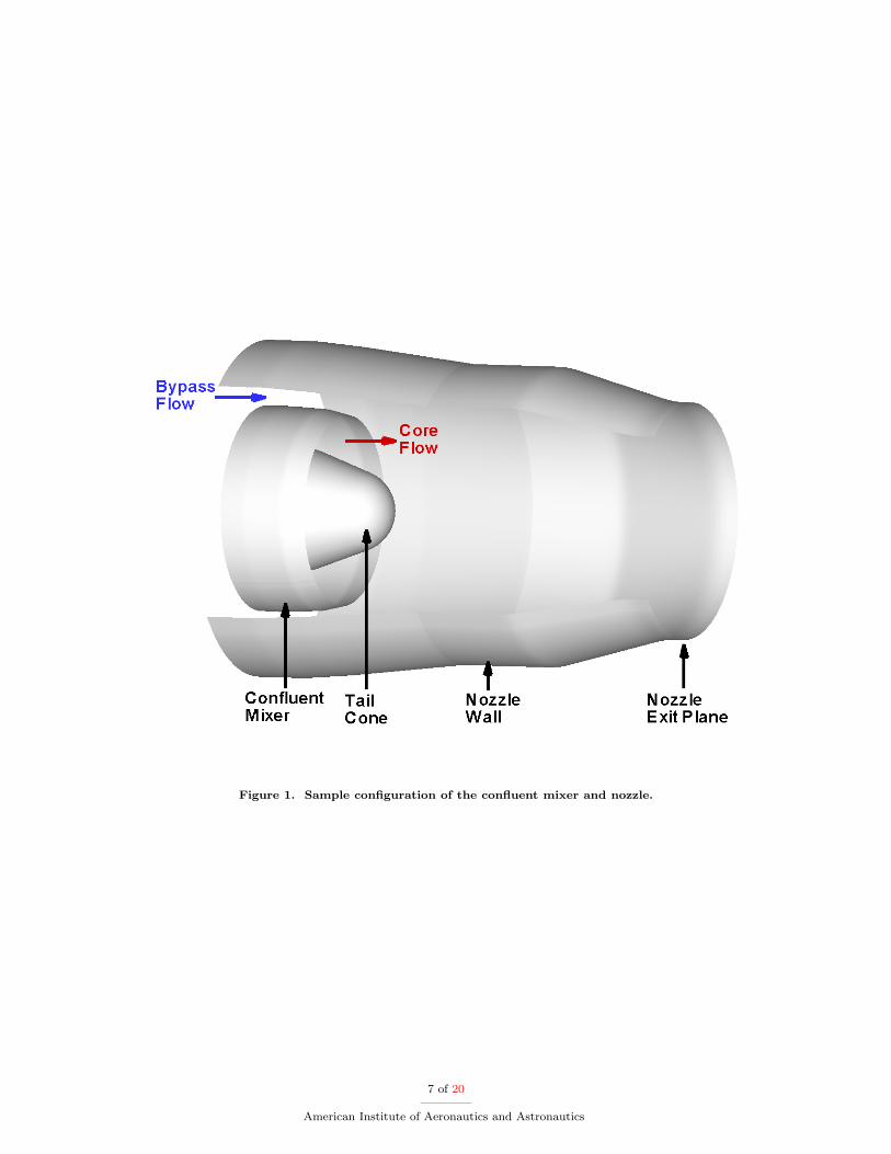
Figure 1. Sample configuration of the confluent mixer and nozzle.

7 of 20


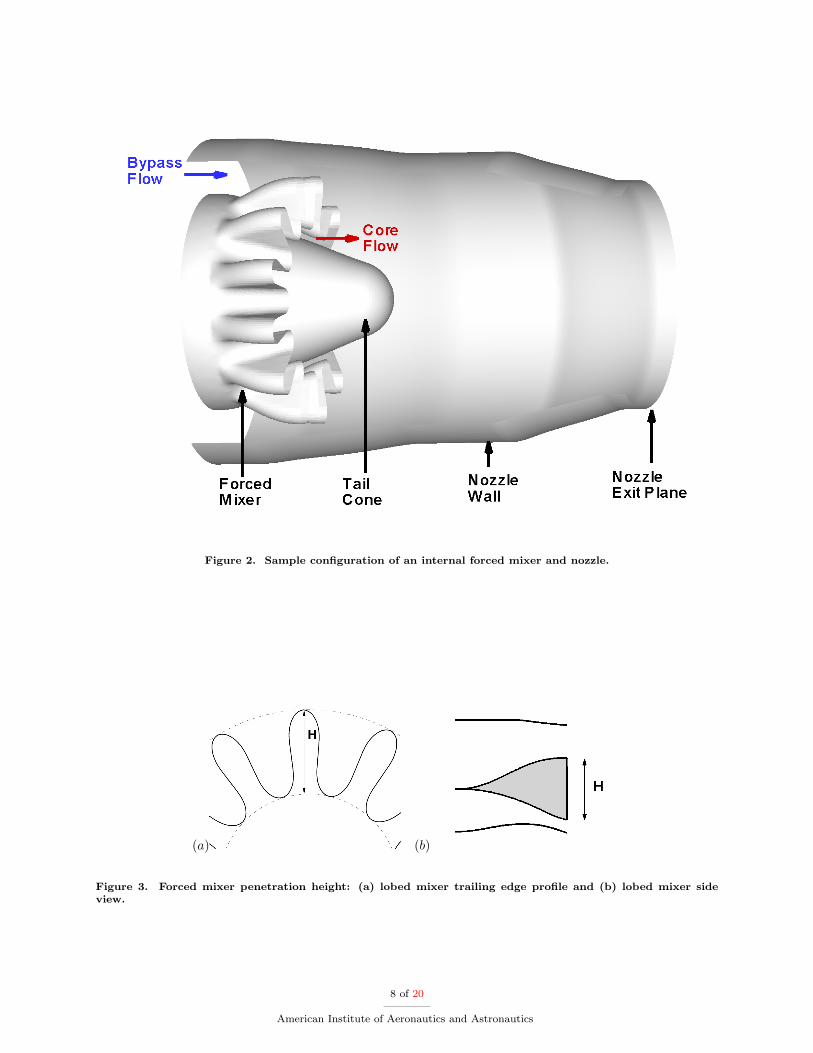
Figure 2. Sample configuration of an internal forced mixer and nozzle.

(a) (b)

Figure 3. Forced mixer penetration height: (a) lobed mixer trailing edge profile and (b) lobed mixer sideview.

8 of 20


Figure 4. Nozzle geometry profiles: (a) L0, L1, and L2 nozzles (b) L2 nozzle (c) L1 nozzle and (d) L0 (baseline)nozzle.

9 of 20


(a)

(b)

Figure 5. CFD and PIV comparison for the confluent mixer at set point 5000: (a) normalized velocity (U/Um)and (b) relative turbulence intensity (k1/2/Um(%)); positive radii, CFD; negative radii, PIV.

10 of 20


(a)

(b)

Figure 6. CFD and PIV comparison for the confluent mixer at set point 312: (a) normalized velocity (U/Um)and (b) relative turbulence intensity (k1/2/Um(%)); positive radii, CFD; negative radii, PIV.

11 of 20


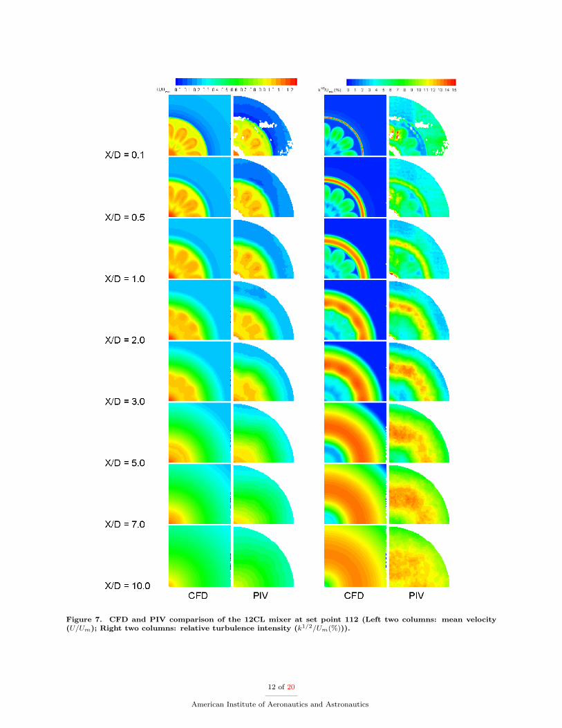
Figure 7. CFD and PIV comparison of the 12CL mixer at set point 112 (Left two columns: mean velocity(U/Um); Right two columns: relative turbulence intensity (k1/2/Um(%))).

12 of 20


(a) (b)

(c) (d)

Figure 8. Comparison of radial profiles of mean velocity (U/Um) in the lobe peak azimuthal plane betweenCFD and PIV for the 12CL mixer at set point 112: (a) X/D=0.1, (b) X/D=1, (c) X/D=5, and (d) X/D=10;solid line, PIV; dash line, CFD.

13 of 20


(a) (b)

(c) (d)

Figure 9. Comparison of radial profiles of relative turbulence intensity (k1/2/Um(%)) in the lobe peak azimuthalplane between CFD and PIV for the 12CL mixer at set point 112: (a) X/D=0.1, (b) X/D=1, (c) X/D=5, and(d) X/D=10; solid line, PIV; dash line, CFD.

14 of 20


Figure 10. CFD relative turbulence intensities (k1/2/Um(%)) of the 12CL, 12UM, and 12UH mixers at setpoint 312.

Figure 11. PIV relative turbulence intensities (k1/2/Um(%)) of the 12CL, 12UM, and 12UH mixers at set point312.

15 of 20


Figure 12. Far-field Sound Pressure Level spectra at 70◦ for the 12UM mixer with the L0 nozzle and the 12CLmixer with the L0, L1, and L2 nozzles at set point 310.

Figure 13. Axial variation of the angle between the interior nozzle wall and the jet axis for the L0, L1, andL2 nozzles.

16 of 20


(a)

(b)

(c)

Figure 14. CFD Mach number contours for the 12UM mixer in the lobe peak azimuthal plane at set point312 with the (a) L0 nozzle, (b) L1 nozzle, and (c) L2 nozzle.

17 of 20


(a) (b)

Figure 15. Axial Mach number variation in lobe peak azimuthal plane of the 12UM mixer with the L0 nozzleat set point 312 (a) Mach number contours and profile locations (b) Mach number profiles (along lines offsetfrom the nozzle wall).

(a) (b)

Figure 16. Axial Mach number variation in lobe peak azimuthal plane of the 12UM mixer with the L1 nozzleat set point 312 (a) Mach number contours and profile locations (b) Mach number profiles (along lines offsetfrom the nozzle wall.

18 of 20


(a) (b) (c)

Figure 17. CFD turbulence kinetic energy upstream of the normal shock for the (a) 12CL mixer, (b) 12UMmixer, and (c) 12UH mixer; bold contours, supersonic region; thin contours, subsonic region.

(a) (b) (c)

Figure 18. Estimated HML noise source strength on the shock surface for the (a) 12CL mixer, (b) 12UMmixer, and (c) 12UH mixer.

19 of 20


Figure 19. Estimated HML noise source peak frequencies for the 12CL mixer at set point 310.

Figure 20. Estimated HML noise source directivity at for the 12CL mixer at set point 310.

20 of 20


computational fluid dynamics analysis of jets with ...lyrintzi/aiaa-2005-2887-loren.pdfcomputational...

Documents