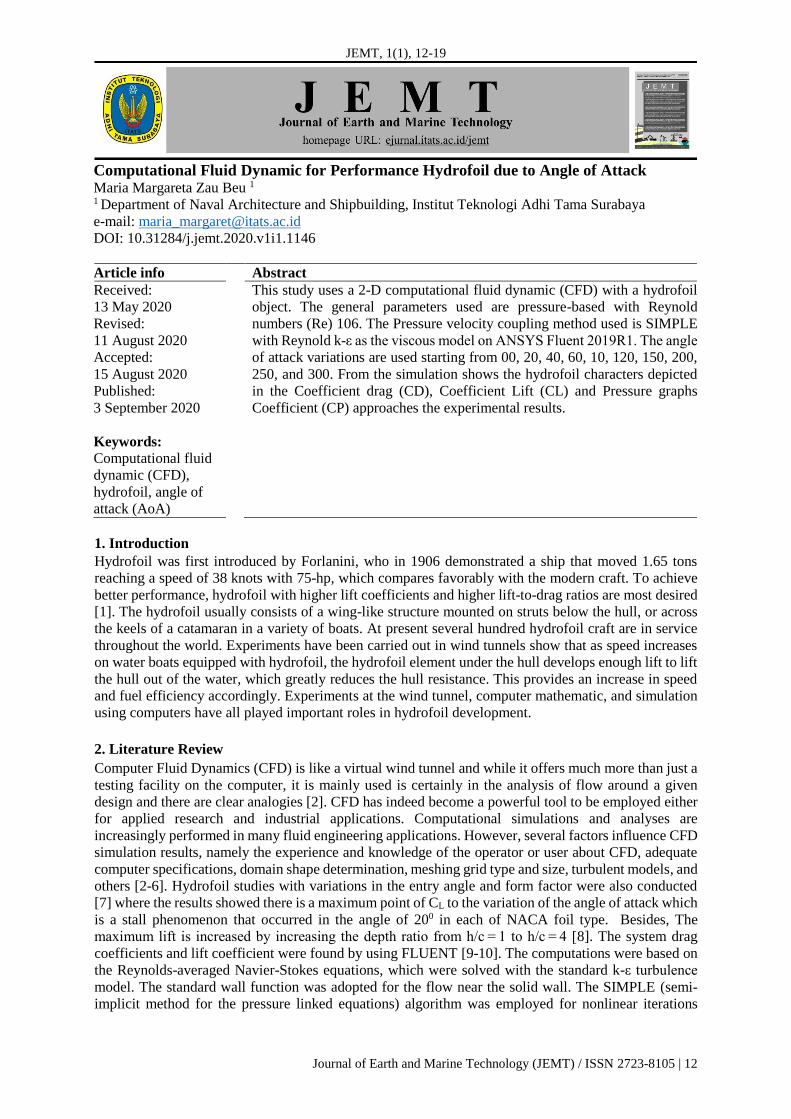
JEMT, 1(1), 12-19

Journal of Earth and Marine Technology (JEMT) / ISSN 2723-8105 | 12

Computational Fluid Dynamic for Performance Hydrofoil due to Angle of Attack Maria Margareta Zau Beu 1

1 Department of Naval Architecture and Shipbuilding, Institut Teknologi Adhi Tama Surabaya e-mail: maria_margaret@itats.ac.id

DOI: 10.31284/j.jemt.2020.v1i1.1146

Article info Abstract

Received:

13 May 2020

Revised:

11 August 2020

Accepted:

15 August 2020

Published:

3 September 2020

Keywords: Computational fluid

dynamic (CFD),

hydrofoil, angle of

attack (AoA)

This study uses a 2-D computational fluid dynamic (CFD) with a hydrofoil

object. The general parameters used are pressure-based with Reynold

numbers (Re) 106. The Pressure velocity coupling method used is SIMPLE

with Reynold k-ε as the viscous model on ANSYS Fluent 2019R1. The angle

of attack variations are used starting from 00, 20, 40, 60, 10, 120, 150, 200,

250, and 300. From the simulation shows the hydrofoil characters depicted

in the Coefficient drag (CD), Coefficient Lift (CL) and Pressure graphs

Coefficient (CP) approaches the experimental results.

1. Introduction

Hydrofoil was first introduced by Forlanini, who in 1906 demonstrated a ship that moved 1.65 tons

reaching a speed of 38 knots with 75-hp, which compares favorably with the modern craft. To achieve

better performance, hydrofoil with higher lift coefficients and higher lift-to-drag ratios are most desired

[1]. The hydrofoil usually consists of a wing-like structure mounted on struts below the hull, or across

the keels of a catamaran in a variety of boats. At present several hundred hydrofoil craft are in service

throughout the world. Experiments have been carried out in wind tunnels show that as speed increases

on water boats equipped with hydrofoil, the hydrofoil element under the hull develops enough lift to lift

the hull out of the water, which greatly reduces the hull resistance. This provides an increase in speed

and fuel efficiency accordingly. Experiments at the wind tunnel, computer mathematic, and simulation

using computers have all played important roles in hydrofoil development.

2. Literature Review

Computer Fluid Dynamics (CFD) is like a virtual wind tunnel and while it offers much more than just a

testing facility on the computer, it is mainly used is certainly in the analysis of flow around a given

design and there are clear analogies [2]. CFD has indeed become a powerful tool to be employed either

for applied research and industrial applications. Computational simulations and analyses are

increasingly performed in many fluid engineering applications. However, several factors influence CFD

simulation results, namely the experience and knowledge of the operator or user about CFD, adequate

computer specifications, domain shape determination, meshing grid type and size, turbulent models, and

others [2-6]. Hydrofoil studies with variations in the entry angle and form factor were also conducted

[7] where the results showed there is a maximum point of CL to the variation of the angle of attack which

is a stall phenomenon that occurred in the angle of 200 in each of NACA foil type. Besides, The

maximum lift is increased by increasing the depth ratio from h/c = 1 to h/c = 4 [8]. The system drag

coefficients and lift coefficient were found by using FLUENT [9-10]. The computations were based on

the Reynolds-averaged Navier-Stokes equations, which were solved with the standard k-ε turbulence

model. The standard wall function was adopted for the flow near the solid wall. The SIMPLE (semi-

implicit method for the pressure linked equations) algorithm was employed for nonlinear iterations

Journal of Earth and Marine Technology (JEMT) / ISSN 2723-8105 | 13

between the velocity and pressure fields [11]. The iterative formulations of the SIMPLE methods

generally exhibit better behavior [12]. SIMPLE typically converges very fast and efficiently, but for

industrial flows in complex geometries and with marginal flow stability, convergence may stall.

3. Research Method

3.1 Computational Approach

Computational fluid dynamics (CFD) is based on three basic physical principles: conservation of mass,

momentum, and energy. The governing equations in CFD are based on these conservation principles.

The continuity equation 2-D is based on the conservation of mass for an incompressible fluid.

0)()(

y

v

x

u

t

(1)

The turbulence model widely used in CFD is k-ε model. The transported turbulent quantities of the k-ε

model have physical meaning. The first variable is the turbulent kinetic energy k

)''''''(2

1wwvvuuk (2)

The second variable is the viscous dissipation rate ε which governs the dissipation of turbulent kinetic

energy due to the shearing of the smallest eddies

ijij eev ''2 (3)

ε is given per unit mass. A velocity scale can conveniently be taken from kuref , similarly, a length

scale is obtained from /2/3kl and the eddy viscosity then becomes

2kCluC refT (4)

When 1,,, CC kand 2C . These constants have been arrived at by comprehensive data fitting for

a wide range of turbulent flows,

92.1,44.1,3.1,0.1,09,0 21 CCC ek

For the k-ε model incoming turbulence was specified through turbulent intensity at 5% and turbulent

viscosity ratio at a value of 10.

3.2 Lift and Drag Coefficient

Lift is generated on a foil in a flow, the force working in the normal direction on the flow. The magnitude

of the angle of the lift will depend on the angle of attack, the thickness, hydrofoil, and the camber. In

addition to the lift force, there will be a drag force that works in the flow direction, this is mostly due to

viscous effects.

Figure 1. 2D-foil geometry definition[13] Figure 2. 2D-foil with the angle of attack [13]

AU

LC

water

L 2

2

(5)

AU

DC

water

D 2

2

(6)

Journal of Earth and Marine Technology (JEMT) / ISSN 2723-8105 | 14

where the characteristic area A corresponds to the hydrofoil planform area for a horizontally oriented,

completely submerged hydrofoil. Value for pressure coefficient (CP) is,

PP

PP

V

PPCP

0

25.0 (7)

Where, P is the static pressure at the point at which the pressure coefficient is being evaluated, P is

the static pressure in the freestream, 0P is the stagnation pressure in the freestream, is the

freestream fluid density, 2

V is the freestream velocity of the fluid, or the velocity of the body through

the fluid [14-15].

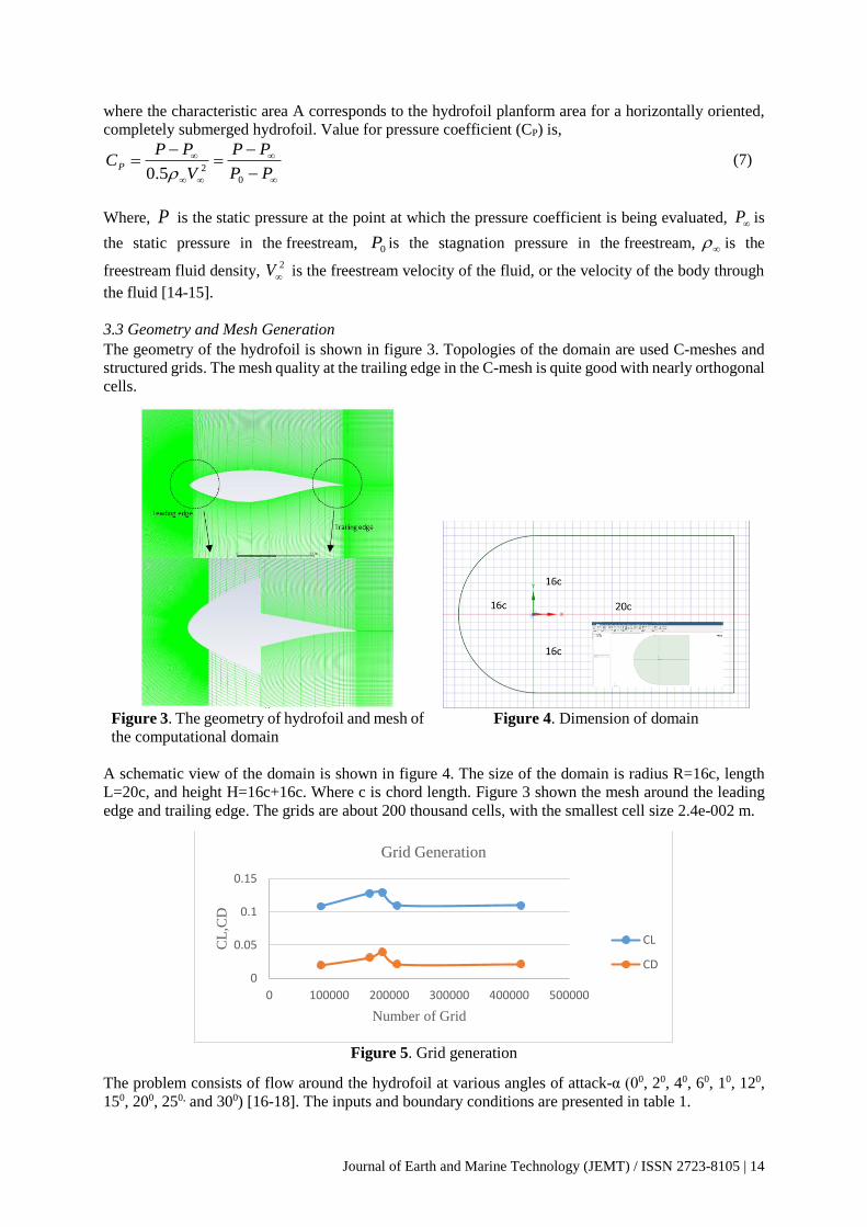
3.3 Geometry and Mesh Generation

The geometry of the hydrofoil is shown in figure 3. Topologies of the domain are used C-meshes and

structured grids. The mesh quality at the trailing edge in the C-mesh is quite good with nearly orthogonal

cells.

Figure 3. The geometry of hydrofoil and mesh of

the computational domain

Figure 4. Dimension of domain

A schematic view of the domain is shown in figure 4. The size of the domain is radius R=16c, length

L=20c, and height H=16c+16c. Where c is chord length. Figure 3 shown the mesh around the leading

edge and trailing edge. The grids are about 200 thousand cells, with the smallest cell size 2.4e-002 m.

Figure 5. Grid generation

The problem consists of flow around the hydrofoil at various angles of attack-α (00, 20, 40, 60, 10, 120,

150, 200, 250, and 300) [16-18]. The inputs and boundary conditions are presented in table 1.

0

0.05

0.1

0.15

0 100000 200000 300000 400000 500000

CL

,CD

Number of Grid

Grid Generation

CL

CD

Journal of Earth and Marine Technology (JEMT) / ISSN 2723-8105 | 15

Table 1. Inputs and Boundary Condition

General Parameter

Solver

State

Viscous Model

Material

Density

Reynold Number (Re)

Inlet Velocity

Chord Length

Pressure-Velocity Coupling

Pressure based

Steady

Reynold k-epsilon (ε)

Water

1000 kg/m3

106

10 knot

1 m

SIMPLE

4. Result and Analysis

The numerical method used here had been validated in the experimental study. The result is presented

in Figures 26 and 27.

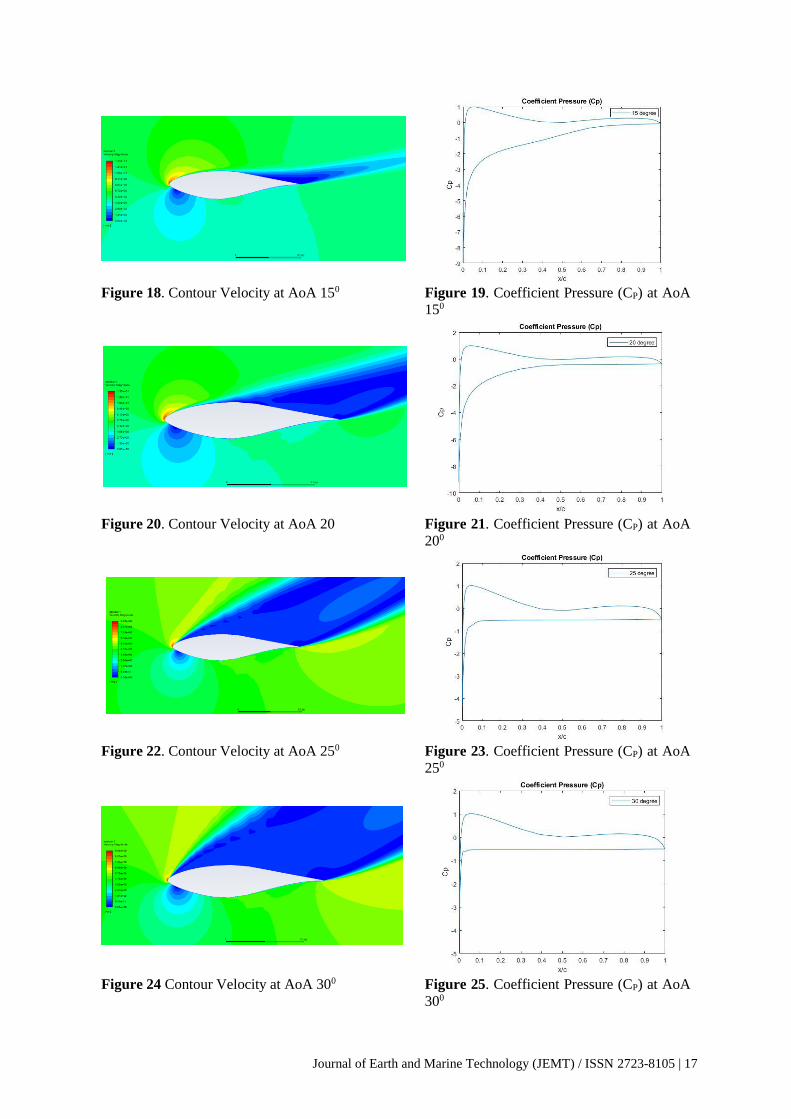
4.1 Contour Velocity and Pressure Coefficient

Hydrofoil performance obtained through the CFD approach with a fluid (water) velocity of 5.14 m/s or

equivalent to 10 knots with variations angle of attack (AoA)-α, shows the boundary layer and wake

increase in thickness with increasing angle of attack. The pressure coefficient of the hydrofoil’s upper

surface was positive and the lower surface was negative. The coefficient of pressure difference is much

larger on the leading edge, while on the rear/trailing edge it was much lower.

Figure 6. Contour Velocity at AoA 00 Figure 7. Coefficient Pressure (CP) at AoA

00

Figure 8. Contour Velocity at AoA 20 Figure 9. Coefficient Pressure (CP) at AoA 20

Journal of Earth and Marine Technology (JEMT) / ISSN 2723-8105 | 16

Figure 10. Contour Velocity at AoA 40 Figure 11. Coefficient Pressure (CP) at AoA

40

Figure 12. Contour Velocity at AoA 60 Figure 13. Coefficient Pressure (CP) at AoA

60

Figure 14. Contour Velocity at AoA 100

Figure 15. Coefficient Pressure (CP) at AoA

100

Figure 16. Contour Velocity at AoA 120 Figure 17. Coefficient Pressure (CP) at AoA

120

Journal of Earth and Marine Technology (JEMT) / ISSN 2723-8105 | 17

Figure 18. Contour Velocity at AoA 150

Figure 19. Coefficient Pressure (CP) at AoA

150

Figure 20. Contour Velocity at AoA 20 Figure 21. Coefficient Pressure (CP) at AoA

200

Figure 22. Contour Velocity at AoA 250

Figure 23. Coefficient Pressure (CP) at AoA

250

Figure 24 Contour Velocity at AoA 300 Figure 25. Coefficient Pressure (CP) at AoA

300

Journal of Earth and Marine Technology (JEMT) / ISSN 2723-8105 | 18

The invalidation test case, the lift, and the drag coefficients are compared with experimental data.

Viscous model k-ε turbulence show very good agreement for the angle of attack of up to about 00-150

and 200-250 stalls occur and increase again at an angle of attack 300.

Figure 26. Lift Coefficient (CL) for Hydrofoil in

Various of Angle of Attack

Figure 27. Drag Coefficient (CD) for

Hydrofoil in Various of Angle of Attack

Difference values from experiments and CFD simulations, for the lift coefficient (CL), the average error

is obtained 0.1337 and for the drag coefficient (CD) average error is obtained 0.0374.

6. Conclusion From the result and analysis, 2D-hydrofoil simulation with the angle of attack variations are used starting

from 00, 20, 40, 60, 10, 120, 150, 200, 250, and 300 with the constant Reynolds number 106 using realized

k-ε turbulence model. The Pressure velocity coupling method used is SIMPLE. It is seen that with the

help of CFD Ansys-Fluent software, successful analysis of the Hydrofoil performance has been carried

at various angles of attack (AoA) - α (00, 20, 40, 60, 100, 120, 150, 200, 250, 300) with constant Reynolds

number 106 using the k-ε turbulence model. The boundary layer and wake increase in thickness with

increasing angle of attack. In future works, more realistic environmental hydrodynamic conditions will

be considered for practical investigation, including the shear flow with an exponential profile and the

free-surface waves.

Acknowledgment

The numerical study was conducted at Departement System Engineering and Naval Architecture,

National Taiwan Ocean University, Taiwan. The university provides facilities and support during the

research.

References

[1] Müller, J. D. (2015). Essentials of computational fluid dynamics. In Essentials of Computational

Fluid Dynamics. https://doi.org/10.5860/choice.196614

[2] Zau Beu, M. M., & Kusuma, I. P. A. I. (2017). Investigasi Numerik VIV (Vortex Induced

Vibration) Pada Diameter Kabel Hydrophone 0.04 M Sistem Akustik Bawah Air. ROTOR, 10(2),

47. https://doi.org/10.19184/rotor.v10i2.6387

[3] Pranatal, E., & Beu, M. M. Z. (2018). Analisa CFD Penggunaan Duct pada Turbin Kombinasi

Darrieus-Savonius. Jurnal IPTEK. https://doi.org/10.31284/j.iptek.2018.v22i1.239

[4] Marchand, J. B., Astolfi, J. A., & Bot, P. (2017). Discontinuity of lift on a hydrofoil in reversed

flow for tidal turbine application. European Journal of Mechanics, B/Fluids, 63, 90–99.

https://doi.org/10.1016/j.euromechflu.2017.01.016

[5] Liu, Z., Qu, H., & Shi, H. (2019). Performance evaluation and enhancement of a semi-activated

flapping hydrofoil in shear flows. Energy, 189, 116255.

https://doi.org/10.1016/j.energy.2019.116255

Journal of Earth and Marine Technology (JEMT) / ISSN 2723-8105 | 19

[6] Stern, F., Wang, Z., Yang, J., Sadat-Hosseini, H., Mousaviraad, M., Bhushan, S., Grenestedt, J. L.

(2015). Recent progress in CFD for naval architecture and ocean engineering. Journal of

Hydrodynamics, 27(1), 1–23. https://doi.org/10.1016/S1001-6058(15)60452-8

[7] Putranto, T., & Sulisetyono, A. (2017). Lift-drag coefficient and form factor analyses of hydrofoil

due to the shape and angle of attack. International Journal of Applied Engineering Research,

12(21), 11152–11156

[8] Amini, Y., Kianmehr, B., & Emdad, H. (2019). Dynamic stall simulation of a pitching hydrofoil

near free surface by using the volume of fluid method. Ocean Engineering.

https://doi.org/10.1016/j.oceaneng.2019.106553

[9] ANSYS-Fluent 2019R1 software

[10] Elmekawy, A. N., Introduction to ANSYS Meshing Module-01

[11] Wu, J. T., Chen, J. H., Hsin, C. Y., & Chiu, F. C. (2019). Dynamics of the FKT System with

Different Mooring Lines. Polish Maritime Research, 26(1), 20–29. https://doi.org/10.2478/pomr-

2019-0003

[12] Vandoormaal, J.P., Raithby, G.D., 1984. Enhancements of the SIMPLE method for predicting

incompressible fluid flows. Numer. Heat Transf. 7, 147–163.

[13] Dagestad, I. (2018). Actuation moments for hydrofoil flaps, Norwegian University of Science and

Technology, Department of Marine Technology

[14] Newman, J. N., (1977). Marine Hydrodynamics, MIT.

[15] White, F.M., 2011. Fluid Mechanics, seventh ed. McGraw-Hill, New York, USA.

[16] Giesing, J.P., Smith, A.M.O., 1967. Potential flow about two-dimensional hydrofoils. J.

Fluid Mech. 28, 113–129

[17] Ni, Z., Dhanak, M., & Su, T. chow. (2019). Performance of a slotted hydrofoil operating close to

a free surface over a range of angles of attack. Ocean Engineering, 188(June), 106296.

https://doi.org/10.1016/j.oceaneng.2019.106296

[18] Bai, K.J., 1978. A localized finite-element method for two-dimensional steady potential flows with

a free surface. J. Ship Res. 22, 216–230.