computational cosmology - uam
TRANSCRIPT

Computational Cosmology
Habilitationsschrift
zur Erlangung der venia legendifur das Fach Astronomie & Astrophysik
eingereicht an derMathematisch-Naturwissenschaftlichen Fakultat
der Universitat Potsdam
vonDr. Alexander Knebe
(geboren am 31. Januar 1970 in Kiel)
Potsdam, im November 2008


Thesen zur Habilitationsschrift
Computational Cosmology,vorgelegt von Dr. Alexander Knebe
• Numerical simulations of cosmic structure formation follow the evolution of darkmatter (host) haloes and their substructure content, i.e. dark matter subhaloes.
• Dark matter subhaloes are anisotropically distributed, i.e. they are preferentiallyfound along the major axis of their host halo.
• Subhaloes are radially aligned, i.e. their major axis points towards the centre of thehost they orbit in.
• Subhaloes tend to be on orbits co-rotating with their hosts.
• Subhalo-subhalo interactions can lead to significant contributions to the mass loss.
• There exists a prominent population of ”backsplash” galaxies, i.e. galaxies that oncepassed close to the centre of their host but now reside in the outskirts of it.
• Properties of the tidal debris fields from disrupting subhaloes can be related to theparticulars of the subhalo it originates from.
• Even in “live” host halos drawn from cosmological simulations the debris field of dis-rupted subhaloes can be identified as coherent structures in the integrals-of-motionspace.
• However, the relation between host and debris properties is more complex thanderived from controlled experiments of individual subhaloes disrupting in analytical(static) host potentials.
• Warm (instead of cold) dark matter (WDM) greatly reduces the number of subha-loes.
• WDM (sub-)haloes have lower concentrations than their cold dark matter counter-parts.
• WDM leads to a mixture of bottom-up and top-down structure formation, i.e. fila-ments may be fragmenting.
• The likelihood of high-speed encounters akin to the “Bullet” cluster is greater inWDM than in cold dark matter.
• Non-standard inflationary scenarios can lead to “bumps” in the power spectrum ofdensity perturbations; and these bumps may mock different cosmologies, i.e. lead tostructure formation akin to WDM or even open cosmologies.
• Cosmological simulation of cosmic structure formation under the hypothesis of mo-dified Newtonian dynamics (MOND) can lead to a universe comparable to the con-cordance model at redshift z = 0.
• However, the temporal evolution of the number density of objects is different underMOND with very few galaxies present at redshifts z > 3− 5.


Popularwissenschaftliches Abstract zur Habilitationsschrift
Computational Cosmology,vorgelegt von Dr. Alexander Knebe
Die Kosmologie ist heutzutage eines der spannendsten Arbeitsgebiete in der Astronomieund Astrophysik. Das vorherrschende (Urknall-)Modell in Verbindung mit den neuestenund prazisesten Beobachtungsdaten deutet darauf hin, daß wir in einem Universum leben,welches zu knapp 24% aus Dunkler Materie und zu 72% aus Dunkler Energie besteht; diesichtbare Materie macht gerade einmal 4% aus. Und auch wenn uns derzeit eindeutige bzw.direkte Beweise fur die Existenz dieser beiden exotischen Bestandteile des Universums feh-len, so ist es uns dennoch moglich, die Entstehung von Galaxien, Galaxienhaufen und dergroßraumigen Struktur in solch einem Universum zu modellieren. Dabei bedienen sichWissenschaftler Computersimulationen, welche die Strukturbildung in einem expandie-renden Universum mittels Großrechner nachstellen; dieses Arbeitsgebiet wird NumerischeKosmologie bzw. “Computational Cosmology” bezeichnet und ist Inhalt der vorliegendenHabilitationsschrift.Nach einer kurzen Einleitung in das Themengebiet werden die Techniken zur Durchfuhrungsolcher numerischen Simulationen vorgestellt. Die Techniken zur Losung der relevanten(Differential-)Gleichungen zur Modellierung des “Universums im Computer” unterschei-den sich dabei teilweise drastisch voneinander (Teilchen- vs. Gitterverfahren), und es wer-den die verfahrenstechnischen Unterschiede herausgearbeitet. Und obwohl unterschiedli-che Programme auf unterschiedlichen Methoden basieren, so sind die Unterschiede in denEndergebnissen doch (glucklicherweise) vernachlassigbar gering. Wir stellen desweitereneinen komplett neuen Code – basierend auf dem Gitterverfahren – vor, welcher einenHauptbestandteil der vorliegenden Habilitation darstellt.Im weiteren Verlauf der Arbeit werden diverse kosmologische Simulationen vorgestelltund ausgewertet. Dabei werden zum einen die Entstehung und Entwicklung von Satel-litengalaxien – den (kleinen) Begleitern von Galaxien wie unserer Milchstraße und derAndromedagalaxie – als auch Alternativen zum oben eingefuhrten “Standardmodell” derKosmologie untersucht. Es stellt sich dabei heraus, daß keine der (hier vorgeschlagenen)Alternativen eine bedrohliche Konkurenz zu dem Standardmodell darstellt. Aber nichts-destoweniger zeigen die Rechnungen, daß selbst so extreme Abanderungen wie z.B. modi-fizierte Newton’sche Dynamik (MOND) zu einem Universum fuhren konnen, welches dembeobachteten sehr nahe kommt.Die Ergebnisse in Bezug auf die Dynamik der Satellitengalaxien zeigen auf, daß die Un-tersuchung der Trummerfelder von durch Gezeitenkrafte zerriebenen SatellitengalaxienRuckschlusse auf Eigenschaften des ursprunglichen Satelliten zulassen. Diese Tatsachewird bei der Aufschlusselung der Entstehungsgeschichte unserer eigenen Milchstraße vonerheblichem Nutzen sein. Trotzdem deuten die hier vorgestellten Ergebnisse auch daraufhin, daß dieser Zusammenhang nicht so eindeutig ist, wie er zuvor mit Hilfe kontrollierterEinzelsimulationen von Satellitengalaxien in analytischen “Mutterpotentialen” vorherge-sagt wurde: Das Zusammenspiel zwischen den Satelliten und der Muttergalaxie sowie dieEinbettung der Rechnungen in einen kosmologischen Rahmen sind von entscheidenderBedeutung.


Summary“Computational Cosmology” is the modeling of structure formation in the Universeby means of numerical simulations. These simulations can be considered as the only“experiment” to verify theories of the origin and evolution of the Universe. Over thelast 30 years great progress has been made in the development of computer codes thatmodel the evolution of dark matter (as well as gas physics) on cosmic scales and newresearch discipline has established itself.
After a brief summary of cosmology we will introduce the concepts behind such simu-lations. We further present a novel computer code for numerical simulations of cosmicstructure formation that utilizes adaptive grids to efficiently distribute the work andfocus the computing power to regions of interests, respectively. In that regards we alsoinvestigate various (numerical) effects that influence the credibility of these simulationsand elaborate on the procedure of how to setup their initial conditions. And as run-ning a simulation is only the first step to modelling cosmological structure formationwe additionally developed an object finder that maps the density field onto galaxiesand galaxy clusters and hence provides the link to observations.
Despite the generally accepted success of the cold dark matter cosmology the modelstill inhibits a number of deviations from observations. Moreover, none of the putativedark matter particle candidates have yet been detected. Utilizing both the novel sim-ulation code and the halo finder we perform and analyse various simulations of cosmicstructure formation investigating alternative cosmologies. These include warm (ratherthan cold) dark matter, features in the power spectrum of the primordial density per-turbations caused by non-standard inflation theories, and even modified Newtoniandynamics. We compare these alternatives to the currently accepted standard modeland highlight the limitations on both sides; while those alternatives may cure some ofthe woes of the standard model they also inhibit difficulties on their own.
During the past decade simulation codes and computer hardware have advanced to sucha stage where it became possible to resolve in detail the sub-halo populations of darkmatter halos in a cosmological context. These results, coupled with the simultaneousincrease in observational data have opened up a whole new window on the concordancecosmogony in the field that is now known as “Near-Field Cosmology”. We will presentan in-depth study of the dynamics of subhaloes and the development of debris oftidally disrupted satellite galaxies.1 Here we postulate a new population of subhaloesthat once passed close to the centre of their host and now reside in the outer regionsof it. We further show that interactions between satellites inside the radius of theirhosts may not be negliable. And the recovery of host properties from the distributionand properties of tidally induced debris material is not as straightforward as expectedfrom simulations of individual satellites in (semi-)analytical host potentials.
1For the purposes of our studies, we treat “substructure haloes” (or subhaloes) and “satellite galax-ies” as interchangeable. However, we note that the correspondence between dark matter substructuresand luminous satellite galaxies is not a straightforward one.


PrefaceThe concept of this thesis is to present (part of) my cumulative work of the last decadein a thematically ordered fashion. While the key note of the research presented here isobviously computational cosmology it will be divided into the following sub-categories
• cosmological simulations (Section II),
• alternative cosmologies (Section III), and
• near-field cosmology (Section IV).
However, the thesis starts with a general introduction to cosmology in Section I wherethe currently accepted standard model alongside the terminology used throughout thisthesis will be defined. The subsequent Sections are then summaries of my own con-tributions to the respective fields. To this extent I will give an introduction at thebeginning of each Section motivating the scientific relevance and then present one par-ticular highlight of each paper published by myself in that particular area. The papersthat made it into this thesis are the following (ordered chronologically):
(1) Knebe A., Green A., Binney J.J., 2001, MNRAS 325, 845
(2) Knebe A., Islam R.R., Silk J., 2002, MNRAS 326, 109
(3) Knebe A., Devriendt J.E.G., Mahmood A., Silk J., 2002, MNRAS 329, 813
(4) Binney J.J., Knebe A., 2002, MNRAS 333, 378
(5) Little B., Knebe A., Gibson B.K., 2003, MNRAS 341, 617
(6) Knebe A., Devriendt J.E.G., Gibson B.K., Silk J., 2003, MNRAS 345, 1285
(7) Dominguez A., Knebe A., 2003, EpL 4, 631
(8) Knebe A., Dominguez A., 2003, PASA 20, 173
(9) Knebe A., Gill S.P.D., Gibson B.K., 2004, PASA 21, 216
(10) Knebe A., Gibson B.K., 2004, MNRAS 347, 1055
(11) Knebe A., Gill S.P.D., Gibson B.K., Lewis G.F., Ibata R.A., Dopita M.A., 2004, ApJ 603, 7
(12) Gill S.P.D., Knebe A., Gibson B.K., 2004, MNRAS 351, 399
(13) Gill S.P.D., Knebe A., Gibson B.K., Dopita M.A., 2004, MNRAS 351, 410
(14) Gill S.P.D., Knebe A., Gibson B.K., 2005, MNRAS 356, 1327
(15) Knebe A., 2005, PASA 22, 184
(16) Knebe A., Gill S.P.D., Kawata D., Gibson B.K., 2006, 357, 35
(17) Power C.B., Knebe A., 2006, MNRAS 370, 691
(18) Knebe A., Power C.B., Gill S.P.D., Gibson B.K., 2006, MNRAS 368, 1209
(19) Warnick K., Knebe A., 2006, MNRAS 369, 1253
(20) Knebe A., Dominguez A., Dominguez-Tenreiro R., 2006, MNRAS 371, 1959
(21) Knebe A., Arnold B., Power C., Gibson B.K., 2008, MNRAS 386, 1029
(22) Warnick K., Knebe A., Power C.B., 2008, MNRAS 385, 1859
(23) Knebe A., Draganova N., Power C., Yepes G., Hoffman Y., Gottlober S., Gibson B.K., 2008,
MNRAS 386, L52
(24) Knebe A., Yahagi H., Kase H., Lewis G.F., Gibson B.K., 2008, MNRAS 388, L34
This list is not exhaustive and the total number of peer-reviewed papers published bymyself during the years 2001 - 2008 (i.e. after my PhD) is 33 with four more alreadysubmitted. The papers excluded from this thesis are mainly in-depth investigations ofthe properties of galaxies, galaxy clusters, superclusters, and the large-scale clusteringpatterns forming within the standard cold dark matter paradigm.


Contents
I Introduction 1I.1 Cosmology . . . . . . . . . . . . . . . . . . . . . . . . . . . . . . . . . . 2I.2 Friedmann Equations . . . . . . . . . . . . . . . . . . . . . . . . . . . . 3I.3 Structure Formation . . . . . . . . . . . . . . . . . . . . . . . . . . . . 4
I.3.1 The Nature of Dark Matter . . . . . . . . . . . . . . . . . . . . 4I.3.2 Collisionless Matter . . . . . . . . . . . . . . . . . . . . . . . . . 5
I.4 ΛCDM: Concordance Model of Cosmology . . . . . . . . . . . . . . . . 6
II Cosmological Simulations 7II.1 Introduction . . . . . . . . . . . . . . . . . . . . . . . . . . . . . . . . . 8
II.1.1 The Necessity for Cosmological Simulations . . . . . . . . . . . 8II.1.2 The History of Cosmological Simulations . . . . . . . . . . . . . 8II.1.3 The State-of-the-Art of Cosmological Simulations . . . . . . . . 9
II.2 The N -body Concept . . . . . . . . . . . . . . . . . . . . . . . . . . . . 11II.3 Newtonian Mechanics in Comoving Coordinates . . . . . . . . . . . . . 12II.4 Poisson Solver . . . . . . . . . . . . . . . . . . . . . . . . . . . . . . . . 14
II.4.1 Tree Codes . . . . . . . . . . . . . . . . . . . . . . . . . . . . . 14II.4.2 Particle-Mesh Codes . . . . . . . . . . . . . . . . . . . . . . . . 15II.4.3 Hybrid Methods . . . . . . . . . . . . . . . . . . . . . . . . . . . 17II.4.4 Mass Resolution . . . . . . . . . . . . . . . . . . . . . . . . . . . 17II.4.5 Comparison . . . . . . . . . . . . . . . . . . . . . . . . . . . . . 18
II.5 Numerical Issues . . . . . . . . . . . . . . . . . . . . . . . . . . . . . . 19II.5.1 Two-Body Relaxation . . . . . . . . . . . . . . . . . . . . . . . 19II.5.2 Finite Box Size Effects . . . . . . . . . . . . . . . . . . . . . . . 20II.5.3 Hydrodynamics Approach to the Evolution of Cosmic Structure 20
II.6 MLAPM – Multi-Level-Adaptive-Particle-Mesh . . . . . . . . . . . . . . . . . 23II.6.1 Handling Adaptive Meshes . . . . . . . . . . . . . . . . . . . . . 23II.6.2 Generating Refinements . . . . . . . . . . . . . . . . . . . . . . 25II.6.3 Mass Assignment Scheme . . . . . . . . . . . . . . . . . . . . . 27II.6.4 Solving Poisson’s Equation . . . . . . . . . . . . . . . . . . . . . 27
II.7 Halo Finding . . . . . . . . . . . . . . . . . . . . . . . . . . . . . . . . 29II.7.1 Friends-Of-Friends . . . . . . . . . . . . . . . . . . . . . . . . . 29II.7.2 DENMAX/SKID . . . . . . . . . . . . . . . . . . . . . . . . . . 29II.7.3 Bound-Density-Maxima . . . . . . . . . . . . . . . . . . . . . . 30II.7.4 MLAPM’s-Halo-Finder . . . . . . . . . . . . . . . . . . . . . . . . . 30
II.8 Initial Conditions . . . . . . . . . . . . . . . . . . . . . . . . . . . . . . 34II.8.1 Generating Cosmological Initial Conditions . . . . . . . . . . . . 34II.8.2 The Reliability of Cosmological Initial Conditions . . . . . . . . 35

viii CONTENTS
III Alternative Cosmologies 37III.1 Introduction . . . . . . . . . . . . . . . . . . . . . . . . . . . . . . . . . 38III.2 Warm Dark Matter . . . . . . . . . . . . . . . . . . . . . . . . . . . . . 39
III.2.1 The Overabundance of Satellite Galaxies . . . . . . . . . . . . . 39III.2.2 The dynamics of subhaloes in WDM models . . . . . . . . . . . 41III.2.3 Top-Down Fragmentation of WDM Filaments . . . . . . . . . . 42
III.3 Bumpy Power Spectra . . . . . . . . . . . . . . . . . . . . . . . . . . . 44III.3.1 Mocking different Cosmologies . . . . . . . . . . . . . . . . . . . 44III.3.2 Bumpy Power Spectra vs. WDM . . . . . . . . . . . . . . . . . 45
III.4 Modified Newtonian Dynamics . . . . . . . . . . . . . . . . . . . . . . . 47
IV Near-Field Cosmology 51IV.1 Introduction . . . . . . . . . . . . . . . . . . . . . . . . . . . . . . . . . 52
IV.1.1 The Simulations . . . . . . . . . . . . . . . . . . . . . . . . . . . 53IV.1.2 The Haloes . . . . . . . . . . . . . . . . . . . . . . . . . . . . . 53
IV.2 Satellite Galaxies . . . . . . . . . . . . . . . . . . . . . . . . . . . . . . 53IV.2.1 The Dynamics of Satellite Galaxies . . . . . . . . . . . . . . . . 54IV.2.2 The Spatial Anisotropy of Satellite Galaxies . . . . . . . . . . . 56IV.2.3 The Radial Alignment of Satellite Galaxies . . . . . . . . . . . . 57IV.2.4 Backsplash Galaxies: a new population . . . . . . . . . . . . . . 59IV.2.5 The Importance of Satellite-Satellite Interactions . . . . . . . . 60IV.2.6 The Sense of Rotation of Satellite Galaxies . . . . . . . . . . . . 62
IV.3 Debris from Satellite Galaxies . . . . . . . . . . . . . . . . . . . . . . . 63IV.3.1 Mapping Substructures . . . . . . . . . . . . . . . . . . . . . . . 64IV.3.2 Tidal Streams of Disrupting Subhaloes . . . . . . . . . . . . . . 65
V Conclusions & Outlook 69V.1 Conclusions . . . . . . . . . . . . . . . . . . . . . . . . . . . . . . . . . 70V.2 Outlook . . . . . . . . . . . . . . . . . . . . . . . . . . . . . . . . . . . 72
Bibliography 75

Part I
Introduction

2 I.1. COSMOLOGY
I.1 Cosmology
Cosmology - the study of the formation and ultimate fate of structures and galaxiesthroughout the Universe - is without a doubt the dominant field of astrophysics today.And in the last few years theoretical and observational studies have begun to con-verge as we entered the era of “Precision Cosmology”. A picture has emerged in whichcontemporary structures have evolved by gravitational amplification of seed inhomo-geneities that are likely of quantum origin. This picture ties together measurements ofthe cosmic background radiation, estimates of the primordial abundances of the lightelements, measurements of the clustering of galaxies and, to a more limited extent, thecharacteristic properties of individual galaxies (e.g. Komatsu et al., 2008).
There are several turning points to mention that mark the maturation of cosmologyfrom mere speculations to a research discipline. It all began when Einstein formulatedthe theory of general relativity in 1915. It turned out that there are solutions to hisequations that did not comply with the understanding of the Universe at that time,e.g. Friedmann found in 1922 that the Universe cannot be static. Only the pivotaldiscovery of the linear velocity-distance relation for galaxies by Edwin Hubble in 1929changed that perspective. Nevertheless, there was still the prediction of a primordialsingularity for an expanding Universe. Colloquially dubbed “Big Bang” by Fred Hoylein 1949, it was in the year 1965 that Arno Penzias and Robert Wilson discovered whatcan be considered the “remnant fireball of the Big Bang”; they (accidently) observed an“excess antenna temperature” at 4080 Mc/s (Penzias and Wilson, 1965). Already in thesame volume of the Astrophysical Journal Dicke et al. (1965) ascribed a cosmologicalorigin to this radiation, i.e. the cosmic microwave background radiation (CMBR). TheCMBR stems from the epoch when matter and radiation no longer could be in thermalequilibrium due to the cooling arising from the expansion of the Universe: protons andelectrons combined to hydrogen atoms and the Universe became transparant for (theCMBR) photons.
During the 1970’s scientists tried to piece together the jigsaw of how the big bangtheory can give rise to non-linear structures such as galaxies, galaxy groups and clus-ters. And these years also saw the advent of computer simulations of cosmic structureformation to be elaborated upon in Section II. The required primordial density pertur-bations superimposed upon an otherwise homogenous and isotropic Universe were onlydiscovered in 1992 by the COBE2 satellite. COBE found ansiotropies in the CMBRof the order ∆T/T ≈ 10−5, just the right order of magnitude if the majority of thematter in the Universe was so-called “cold dark matter”.3
The following years saw the rise of a wealth of observations targetted at improvedmeasurements of the cosmological parameters; parameters that desribe the evolutionof the Universe as a whole. And these observations converged to what has been calledthe “concordance model of cosmology” to be explained in greater detail in Section I.4.
2Cosmic Microwave Background Explorer3Already at that time it was clear that the rotation curves of individual galaxies as well as the
velocity disperion of galaxies in clusters cannot be explained by luminous matter alone. Additionalmatter that only interacts via gravity was required to explain the inferred gravity.

I.2. FRIEDMANN EQUATIONS 3
I.2 Friedmann Equations
The central equations describing the evolution of the Universe as a whole were firstformulated by Alexander Friedmann in the year 1922. They can be derived fromEinstein’s field equations of general relativity under the assumption of homogeneityand isotropy. In mathematical terms this comes down to using
Gµν + Λg
µν = −8πG
c4T
µν (I.1)
together with the (homogeneous and isotropic) Robertson-Walker metric
ds2 = dt
2− a
2(t)
dr
2
1− kr2+ r
2(dθ2 + sin θ dφ
2)
, (I.2)
where Gµν is the Einstein tensor, T
µν the energy-momentum tensor, Λ the cosmologicalconstant, a(t) the cosmic expansion factor (which determines the overall scale of thespatial metric), and k the curvature parameter.Under the further assumption that the Universe is filled with a perfect fluid (and henceconstraining the energy-momentum tensor correspondingly) one arrives at the followingset of two independent equations, the Friedmann equations :
a
a
2
=
a
a
2
0
Ωr,0a
−4 + Ωm,0a−3 + Ωk,0a
−2 + ΩΛ,0
a =4πG
3a(ρ− ρΛ)
(I.3)
where the density parameters are defined as follows:
Ωr,0 =ρr
ρcrit
Ωm,0 =ρm
ρcrit
Ωk,0 =−k
a20H
20
ΩΛ,0 =ρΛ
ρcrit
(I.4)
The normalisations used in the definitions of the density parameters are as follows
ρcrit =3H2
0
8πG
ρΛ =Λ
8πG
H =a
a
(I.5)
where ρcrit is referred to as the critical density of the Universe (required to obtain aspatially flat universe – in the absence of ρΛ) and H0 is todays value of the Hubbleparameter.

4 I.3. STRUCTURE FORMATION
The solution a(t) to Eq. (I.3) describes the expansion/contraction of the Universe andsensitively depends on these parameters. The determination of these crucial values forcosmology needs to be done observationally and a lot of efforts during the past decadehas been directed towards their confirmation.
I.3 Structure Formation
One of the underlying assumption in the derivation of the Friedmann Eq. (I.3) isthe cosmological principle, i.e. that the Universe is homogenous and isotropic (cf.Robertson-Walker metric Eq. (I.2)). However, this is not what we observe! We seehighly inhomogeneous structures such as galaxies and galaxy clusters alongside thefilamentary structure of the Universe.The just introduced density parameters determine how the Universe as a whole evolvesin time. However, structure formation depends on a couple of more values. Smalldeviations from homegeneity and isotropy need to exist in the early Universe. Theylikely have their origin in quantum fluctuations and are produced in a phase shortlyafter the big-bang called inflation. These fluctuations are thought be of Gaussiannature and can hence be described by a power spectrum. The overall amplitude ofthis power spectrum is yet another parameter to be fixed in order to have a crediblemodel for cosmological structure formation. Further, the shape of the power spectrumof primordial density perturbation also depends on the nature of the (dark) matter.For instance, hot dark matter leads to a different structure formation scenario thancold dark matter: due to its relativistic nature, hot dark matter erase fluctuations onsmall scales and therefore has difficulties to form objects like galaxies whereas colddark matter induces hierarchial structure formation by which small entities form firstand subsequently merge to build larger and larger objects (e.g. Davis et al., 1985).As we will later on return to the nature of dark matter (and actually question it inSection III.1) we are going to elaborate upon the differences in more detail now.
I.3.1 The Nature of Dark Matter
Cold dark matter (CDM) means that dark matter had negligible thermal veloc-ities kT mc
2 in the early universe. As mentioned in, for instance, Primack (2003),this assumption can be satisfied by two complementary sorts of particles:
1. dark matter particles are WIMPs (W eakly Interacting M assive Particles, suchas the neutralino) with mass m ≈ 100Gev and a cross-section of σ ≈ 10−38cm2,
2. dark matter particles are axions with mass m ≈ 10−5ev and hence having non-relativistic velocities kT mc
2, as they do not originate from a thermal mecha-nism in the early universe.
Other authors (e.g. Colın et al., 2000) define a dark matter particle to be cold if andonly if it has a mass of m 1GeV and the strength of its interaction is comparableto the strength of weak interaction.The CDM model is the most favoured in structure formation scenarios first introducedby Peebles (1982) and entails (as already mentioned) hierarchical growth of structures.

I.3. STRUCTURE FORMATION 5
Further, this model is in good agreement with several observations. It correctly pre-dicts the abundances of galaxy clusters nearby and at z ≤ 1. The power spectrumof (primordial) density perturabations is consistent with measurements from CMBanisotropies (Komatsu et al., 2008) and with the flux power spectrum inferred fromLyα forest spectra (Croft et al., 2002).However, there also exist drawbacks that will be expanded upon later on in Sec-tion III.1.
Hot dark matter (HDM) has relativistic thermal velocities kT mc2. Hence,
structures at significant scales up to tens of Mpc’s are “washed out”. This modeltherefore entails fragmentation processes to form structures (cf. Doroshkevich et al.,1974). As this model does not agree with, for instance, the clustering pattern of galaxiesas observed (and simulated) it has been discarded already a long time ago (cf. Peebles,1982; Bond and Szalay, 1983; White et al., 1983). However, we need to mention thatmassive neutrinos are in fact hot dark matter particles. The discrepancy between hotdark matter models and observations thereore places constraints on the allowed massrange for neutrinos.
I.3.2 Collisionless Matter
The different kinds of dark matter have in common to be collisionless, as underlinedby their estimated mean free path λ. Particle physics experiments lead to a WIMP-nucleon elastic-scattering cross section of at minimum σ ≈ 4 × 10−43cm2 at a WIMPmass of 60GeV (cf., e.g., Akerib et al., 2005). Varying the mass m of a dark-matterparticle between 1keV ∼< m ∼< 100GeV induces a number density n of dark matterbetween 1cm−3
∼< n ∼< 6 · 10−8cm−3. Thus, the mean free path of these particles
λ =1
σn∈
1018; 1025
Mpc. (I.6)
is much larger than the Hubble radius
rH =c
H0≈ 4000Mpc, (I.7)
where H0 is todays value of the Hubble parameter (cf. Section I.4).Even when increasing σ in Eq. (I.6) ten orders of magnitude would yield mean freepaths being much greater than rH. Hence, dark matter can be treated as a collisionlessfluid with its phase-space evolution described by the collisionless Boltzmann equation.

6 I.4. ΛCDM: CONCORDANCE MODEL OF COSMOLOGY
I.4 ΛCDM: Concordance Model of Cosmology
Here we simply like to summarize the parameters and their values of the currentlyfavoured (and commonly accepted) standard model of cosmology. The most recentcombination of high-precision measurements of the cosmological parameters presentedin Komatsu et al. (2008) yields
• the matter content Ωm = 0.279• the cosmological constant ΩΛ = 0.721• the Hubble parameter H0 = 70 km/sec/Mpc• the amplitude of density perturbations σ8 = 0.817
and this set of values is referred to as ΛCDM model.
Radiation (parameterized via Ωr) is at a neglegiably low level and hence can be dis-carded. Further, as the sum of all contributions as measured at todays time has to beunity (cf. Eq. (I.3)) the curvature term does not contribute, too.We like to note that these are the latest measurements; the model changed over theyears with minor adjustments of the parameters in one way or the other. Therefore,some of the work presented in this thesis may also refer to open cosmologies (i.e.OCDM, Ωm < 1 & ΩΛ = 0) and the “old” standard cold dark matter model (i.e.SCDM, Ωm = 1 & ΩΛ = 0).

Part II
Cosmological Simulations

8 II.1. INTRODUCTION
This part represents a summary of the following publications:
(1) Knebe A., Green A., Binney J.J., 2001, MNRAS 325, 845(2) Binney J.J., Knebe A., 2002, MNRAS 333, 378(3) Dominguez A., Knebe A., 2003, EpL 4, 631(4) Gill S.P.D., Knebe A., Gibson B.K., 2004, MNRAS 351, 399(5) Knebe A., Dominguez A., 2003, PASA 20, 173(6) Knebe A., 2005, PASA 22, 184(7) Power C.B., Knebe A., 2006, MNRAS 370, 691(8) Knebe A., Dominguez A., Dominguez-Tenreiro R., 2006, MNRAS 371, 1959
II.1 Introduction
As the major theme of this thesis is unbdoubtly “computational cosmology” we decidedto present the concepts behind this rather exciting and novel research field in consid-erable detail. All of the simulations presented later on in Section III and Section IVare though based upon the adaptive mesh refinement technique (cf. Section II.4.2,Section II.4.2 and Section II.6.2). However, we consider it important to highlight andstress the differences between various techniques and the respective codes available to(and used by) the astrophysical community for simulating cosmic structure formation.
II.1.1 The Necessity for Cosmological Simulations
Structure formation is generally believed to be a result of the gravitational amplificationof primordial density perturbations. The amplitude of these initial perturbation thoughhas to have the right value in order to match the clustering patterns observed today.While it is possible to follow the growth of structures to a certain extent using linearperturbation theory (e.g. Zel’dovich, 1970), such calculations are limited and cannotexplain the wealth of observational data available to us; they break down on a scalewhere the (variance of the) density contrast
δ =ρ(x)− ρ
ρ(II.1)
approaches unity. Todays structures exhibit δ-values in the range from voids withδ ≈ −1 to δ ≈ 106 in the central regions of galaxies and larger. This requires the needfor computer simulations: the treatment of perturbations in the non-linear regime is avery complicated problem and the only exact way of doing it is by performing numericalsimulations. As such simulations became more and more sophisticated their relevancefor the field of cosmology has also increased. And today we are left with a resarchbranch on its own, namely computational cosmology to be elaborated upon now.
II.1.2 The History of Cosmological Simulations
The Universe is believed to have started with a Big Bang in which – or more precisely:shortly after which – tiny fluctuations (in an otherwise homogeneous and isotropicspace) were imprinted into the radiation and matter density field. To understand howthe Universe evolved from that early stage into what we observe today (i.e. stars,

II.1. INTRODUCTION 9
galaxies, galaxy clusters, ...) one needs to follow the evolution of those density fieldsusing numerical methods as soon as they turn non-linear (i.e. σδ > 1). Therefore,the approach to cosmological simulations is actually twofold: firstly, one needs togenerate the initial conditions according to the cosmological structure formation modelto be investigated (cf. Section II.8) and secondly, the initial density field (sampled byparticles and hence the reference to N -body codes) needs to be evolved forward in timeusing a numerical integrator for the equations of interest (Sections II.2–II.4).Algorithms have advanced considerably since the first N
2 particle-particle codes (Aarseth,1963; Peebles, 1970; Groth et al., 1977); we have seen the development of the tree-basedgravity solvers (Barnes and Hut, 1986), mesh-based solvers (Klypin and Shandarin,1983), then the two combined (Efstathiou et al., 1985) and multiple strands of adap-tive and deforming grid codes (Villumsen, 1989; Suisalu and Saar, 1995; Kravtsov et al.,1997; Bryan and Norman, 1998; Knebe et al., 2001). While they all push the limitsof efficiency in computational resources, each code has its individual advantages andlimitations. The result of such research has been highly reliable, cost effective codes.In all such codes the evolution is simulated by following the trajectories of particlesunder their mutual gravity. These particles are supposed to sample the matter den-sity field as accurately as possible and a cosmological simulation is nothing more (andnothing less) than a simple and effective tool for investigating non-linear gravitationalevolution. There are two constraints on a cosmological simulation though: a) the cor-rect initial conditions and b) the observation of galaxies, galaxy clusters, large-scalestructure, voids, etc. Simulations are hence trying to bridge the gap between obser-vations of the early Universe (i.e. anisotropies in the Cosmic Microwave Backgroundobserved as early as 300000 years after the Big Bang) and the Universe as we see ittoday.
II.1.3 The State-of-the-Art of Cosmological Simulations
Until now the methods have been continuously refined to allow for more and moreparticles while simultaneously resolving finer and finer structures. Today it is standardto run a cosmological simulation with millions of particles in a couple of days on largesupercomputers or even clusters of PC’s. These simulations can resolve the orbits ofsatellite galaxies within dark matter haloes spanning about five orders of magnitudein mass and spatial dimension (cf. Section IV).Fig. 1 depicts the conceptual ideas behind (cosmological) simulations: starting from ini-tial seed inhomogeneities superimposed onto a homogeneous and isotropic backgroundthe matter field is evolved forward in time. This evolution depends on the cosmologi-cal model under investigation and is performed using an integrator for the appropriateequations describing the physics under investigation. Snapshots of the simulation atvarious times are recorded and then analysed and compared to observational data toverify and falsify theories of structure formation and evolution.
In the following Section we present a brief explanation of the actual name “N -body”code (Section II.2) before transfering the usual (Newtonian) equations of motion into acoordinate system that expands with the Universe in Section II.3. The heart and soulof every N -body code though is the part that solves Poisson’s equation by one meansor the other. We therefore present the general concepts behind the two most popularyet disparate methods to accomplish this task in Section II.4. Before introducing one

10 II.1. INTRODUCTION
Fig. 1. Illustration of the idea driving N -body simulations. Initial conditions (upper left)are being evolved forward in time using a computer programme modeling gravity (and gasphysics) under the assumption of a given cosmological model. The outputs over time are thencompared to observational data and the cosmological model adjusted accordingly. Imagecredit (mass map of Cl0024+164): European Space Agency, NASA and Jean-Paul Kneib(Observatoire Midi-Pyrenees, France/Caltech, USA)
particular N -body in greater detail in Section II.6, we discuss some issues with suchcodes that are of mere numerical nature in Section II.5. The last Section II.8 thendeals with the process of generating the initial conditions for cosmological simulationsand its intrinsic complications.
II.2. THE N-BODY CONCEPT 11
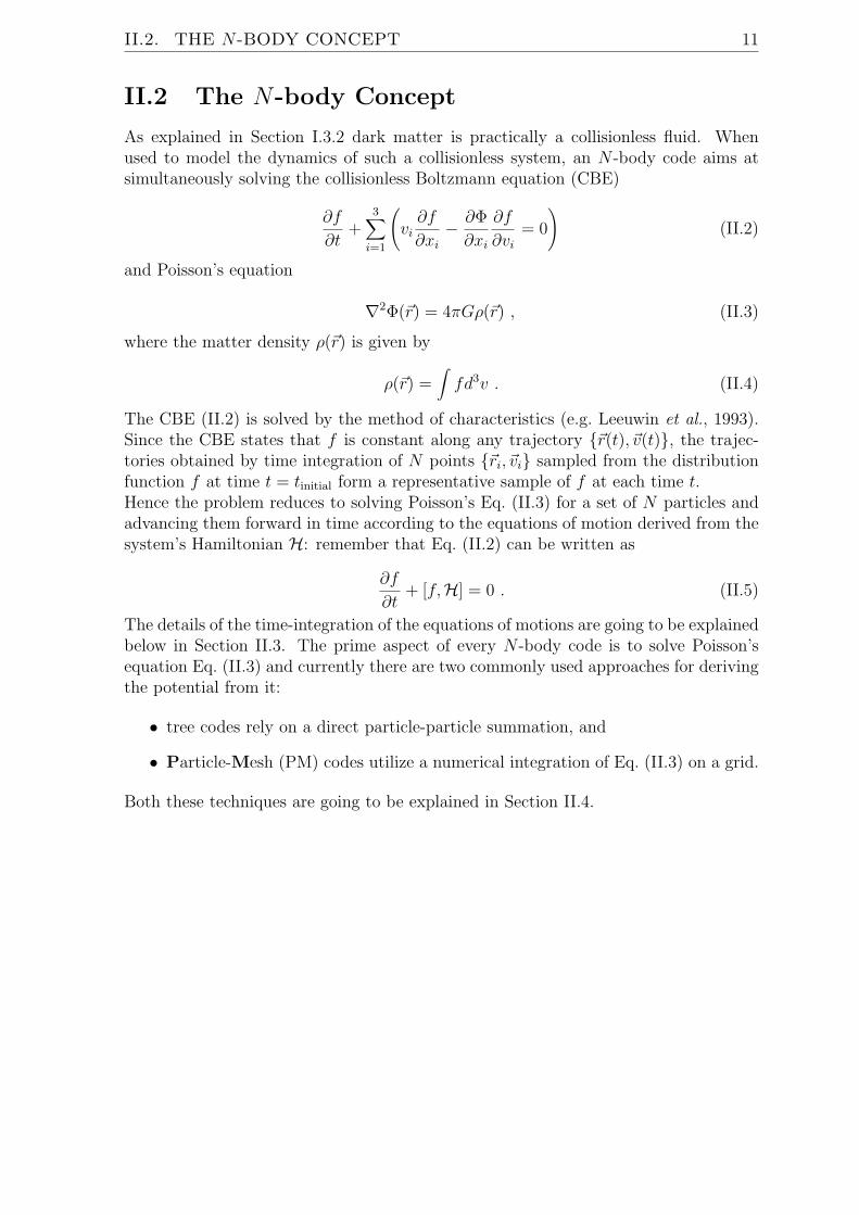
II.2 The N-body Concept
As explained in Section I.3.2 dark matter is practically a collisionless fluid. Whenused to model the dynamics of such a collisionless system, an N -body code aims atsimultaneously solving the collisionless Boltzmann equation (CBE)
∂f
∂t+
3
i=1
vi∂f
∂xi−
∂Φ
∂xi
∂f
∂vi= 0
(II.2)
and Poisson’s equation
∇2Φ(r) = 4πGρ(r) , (II.3)
where the matter density ρ(r) is given by
ρ(r) =
fd3v . (II.4)
The CBE (II.2) is solved by the method of characteristics (e.g. Leeuwin et al., 1993).Since the CBE states that f is constant along any trajectory r(t),v(t), the trajec-tories obtained by time integration of N points ri,vi sampled from the distributionfunction f at time t = tinitial form a representative sample of f at each time t.Hence the problem reduces to solving Poisson’s Eq. (II.3) for a set of N particles andadvancing them forward in time according to the equations of motion derived from thesystem’s Hamiltonian H: remember that Eq. (II.2) can be written as
∂f
∂t+ [f,H] = 0 . (II.5)
The details of the time-integration of the equations of motions are going to be explainedbelow in Section II.3. The prime aspect of every N -body code is to solve Poisson’sequation Eq. (II.3) and currently there are two commonly used approaches for derivingthe potential from it:
• tree codes rely on a direct particle-particle summation, and
• Particle-Mesh (PM) codes utilize a numerical integration of Eq. (II.3) on a grid.
Both these techniques are going to be explained in Section II.4.

12 II.3. NEWTONIAN MECHANICS IN COMOVING COORDINATES
II.3 Newtonian Mechanics in Comoving Coordinates
Even though solving Poisson’s equation is central to every N -body code, it is alsoimportant to accurately update particle positions and velocities, i.e. integrating theequations of motion. And as the Universe is expanding it is convenient to introducecomoving coordinates :
x =r
a(t)(II.6)
where a(t) is the cosmic expansion factor and the solution to the (first) Friedmannequation (I.3).The (comoving) Lagrangian is given by (cf. Knebe et al., 2001)
L = 12a
2x
2−
Φ
a, (II.7)
which leads to the canonical momentum
p = a2x. (II.8)
Hamilton’s equations are therefore
dx
dt=
p
a2
dp
dt= −
∇Φ
a.
(II.9)
accompanied by the Poisson’s equation in comoving coordinates
∆Φ = 4πGa(ρ− ρb) (II.10)
where ρb is the cosmic background density (and hence Φ is the potential responsiblefor “peculiar accelerations”).The equations-of-motion (II.9) can be discretized and integrated using a second-orderaccurate scheme as follows:
xn+1/2 = xn + pn
t+∆t/2
t
dt
a2
pn+1 = pn − ∇Φ(xn+1/2) t+∆t
t
dt
a
xn+1 = xn+1/2 + pn+1
t+∆t
t+∆t/2
dt
a2,
(II.11)
where the integrals can be evaluated analytically as they depend only on the cosmology.This modified leap-frog scheme only needs to store one copy of the positions and veloc-ities whereas other integrators as, for instance, Runge-Kutta consume more memory.Further, it has been shown that symplectic integrators4 such as Eq. (II.11) are bet-ter suited for Hamiltonian systems (Springel, 2005) as they are robust against non-
4Symplectic integrators preserve Poincare integral invariants, or in other words, preserve phase-space.

II.3. NEWTONIAN MECHANICS IN COMOVING COORDINATES 13
Hamiltonian perturbations introduced by, for instance, ordinary numerical integrationmethods.

14 II.4. POISSON SOLVER
II.4 Poisson Solver
As already mentioned in Section II.2 there are two complementary approaches forderiving the potential from Poisson’s equation (II.3): a) tree codes rely on a directparticle-particle summation, and b) PM (particle-mesh) codes utilize a numerical in-tegration of Eq. (II.3) on a grid.
II.4.1 Tree Codes
Fig. 2. Illustration of a tree code. The left panel shows the actual particle distribution andits cubical decomposition. The right panel is the tree corresponding to this distribution.
The Pre-Requisites
The particle-particle (PP) method upon which tree codes are based assumes that theparticles are δ-functions and hence the density field (rhs of Poisson’s Eq. (II.3)) readsas follows:
ρ(r) =N
i=1
miδ(r − ri) , (II.12)
where N is the total number of particles in use.
The Forces
Combining Eq. (II.12) with Eq. (II.3) the analytical solution for the force F at particleposition ri is given by:
F (ri) =
j =i
mimj
|ri − rj|2
ri − rj
|ri − rj|
. (II.13)
But as we are interested in deriving the force at every single particle position, thePP method scales like N
2 (N summations, each over (N − 1) particles). Therefore, a

II.4. POISSON SOLVER 15
(straightforward) PP summation does not appears to be feasible for evolving a set of N
particles under their mutual gravity, not even on the largest supercomputers availablenowadays! One needs to bypass the increase in computational time for large numbersof particles with a more sophisticated treatment when calculating the forces. One wayof achieving this is to organize the particles in a tree-like structure: particles located”far away” from the actual particle (at which position we intend to calculate the force)can be lumped together as a single – but more massive – particle. This tunes downthe number of calculations dramatically.The idea of a tree code is sketched in Fig. 2. The particles are organized in a tree-likestructure based upon a cubical decomposition of the computational domain. Con-sequentially, for each particle we “walk the tree” and add the forces from branchingsthat need no further unfolding into finer branches according some pre-selected “openingcriterion”.One publicly available tree code is called GADGET5 (Galaxies with Dark Matter andGas intEracT) and I refer the reader to a more elaborate discussion of this techniqueto its reference paper by Springel et al. (2001) and Springel (2005).
Force Resolution – softening
In order to avoid the singularity for ri = rj in Eq. (II.13) one needs to set a limit onthe minimal allowed spatial separation between two particles. This can be achieved byintroducing a (fixed) scale, i.e. the softening parameter :
F (ri) =
j =i
mimj
|ri − rj|2 + 2
ri − rj
|ri − rj|
(II.14)
This softening is closely related to the overall force resolution of the simulation and anelaborate discussion of it can be found in Dehnen (2001).
II.4.2 Particle-Mesh Codes
The Pre-Requisites
Another way for obtaining the forces is to numerically integrate Poisson’s equation (II.3).This method, however, demands the introduction of a grid in order to define the den-sity and hence the name particle-mesh (PM) method. The grid is usually of a regular(cubic) shape with L × L × L cells where each cell is identified by the index triplet(i, j, k). The forces are then calculated according to the following scheme:
1. assign all particles to the grid to get ρi,j,k
2. solve Poisson’s equation ∇2φi,j,k = 4πGρi,j,k
3. differentiate to get forces Fi,j,k = −∇φi,j,k
4. interpolate Fi,j,k back to particle positions
5GADGET can be downloaded from this web address http://www.mpa-garching.mpg.de/gadget

16 II.4. POISSON SOLVER
Fig. 3. An example for adaptive mesh refinement. The left panel shows the particle distri-bution at redshift z = 0 in a ΛCDM simulation. The right panel indicates the arbitrarilyshaped grids invoked by the AMR code MLAPM to solve Poisson’s equation. Not that the gridcovering the whole computational domain is not shown for clarity.
The Forces
With this scheme most of the time is spent in step 2 and the most common way tosolve Poisson’s equation on a grid is to make use of FFT’s (Fast-Fourier-Transforms).The analytical solution to Poisson’s equation is given by the integral
Φ(r) =
G(r − r)ρ(r)dr (II.15)
where G(x) = −x/x3/2 is the Green’s function of Poisson’s equation. This integral can
readily be evaluated in Fourier-space, i.e.
Φ = G ρ (II.16)
where Φ, G, and ρ are the Fourier transforms of the respective variables.The PM approach proves to be exceptionally fast outperforming any tree code.There are of course other techniques than the use of FFT’s available to numericallysolve Poisson’s equation but the utilisation of FFT’s is the most common approach asit appears to be the fastest.
Force Resolution – adaptive mesh refinement
The most severe problem with the PM method is the lack of spatial resolution below twogrid spacings. Whereas tree codes require the introduction of a softening length to avoidthe force singularity for close encounters of particles, PM codes suffer from the oppositeproblem. Gravity is an attractive force and hence the particles flow from low densityregions into high density regions amplifying primordial density fluctuations. This leads

II.4. POISSON SOLVER 17
to an excess of particles in certain cells whereas other cells are becoming more and moredevoid of matter. But as the spacing of the grid introduces a (smoothing) scale particlescloser than about two cell distances do not interact according to Eq. (II.15) anymore.We are left with the situation where we can not resolve structure formation on scalesof (and below) roughly the cell spacing of the grid!This is a major problem and the most obvious way to overcome it is to introduce finergrids in regions of high density. These grids though need to freely adapt to the actualparticle distribution at all times and hence navigating such complex grids throughcomputer memory is a very demanding task. One of the freely available adaptivemesh refinement (AMR) codes is MLAPM6 (Knebe et al., 2001).The mode of operation of this AMR technique can be viewed in Fig. 3 where a slicethrough a standard ΛCDM simulation is presented. The left panel shows the distribu-tion of particles whereas the right panel indicates the adaptive meshes used to obtaina solution to Poisson’s equation.It needs to be stressed though that the use of irregularly shaped grids inhibits FFT’s.Another technique for solving Poisson’s equation needs to be sought such as, for in-stance, multi-grid relaxation (e.g. Brandt, 1977; Press et al., 1992; Kravtsov et al.,1997; Knebe et al., 2001).
II.4.3 Hybrid Methods
There are, of course, various other techniques for simultaneously being time efficientand having a credible force resolution. One possibility is realized in the so-called P3Mtechnique (i.e. Couchman, 1991) where a combination of PP and PM provides thenecessary balance between accuracy and efficiency: the force as given by the plain PMcalculation is augmented by a direct summation over all neighboring particles withinthe surrounding cells. This gives accurate forces down to the scale provided by thesoftening parameter again. Other examples, for instance, are Tree-PM (Bode andOstriker, 2003) and moving mesh (Gnedin, 1995) codes, but the details are well beyondthe scope of this thesis.
II.4.4 Mass Resolution
It still needs to be mentioned that a cosmological simulation in practice only simulatesa certain fraction of the Universe. This is what people refer to as the simulation box.However, to account for the fact the Universe is actually infinite one uses periodicboundary conditions: particles leaving the box on one side immediately enter the boxagain on the other side.Moreover, the size of the box also defines the mass resolution of the simulation. Weare only using a certain number of particles within a fixed region of the Universe.And as the density of the Universe is determined by the cosmological model underinvestigation, each individual particle has a certain mass. This mass determines themass resolution of that specific simulation. For instance, if we model the evolutionof about 2 million particles in a box with side length 25h−1Mpc using the ΛCDMcosmology (Ω0 = 0.3), each particle weighs about 6 · 108
h−1
M⊙. Therefore we will notbe able to properly resolve dwarf galaxies in that particular cosmological simulation(Mdwarf ≥ 107
h−1
M⊙).
6MLAPM can be downloaded from this web address http://www.aip.de/People/AKnebe/MLAPM

18 II.4. POISSON SOLVER
II.4.5 Comparison
It only appears natural to ask the question which method is superior and how theycompare, respectively.There is no straight forward answer as both methods have their (dis-)advantages. Treecodes are based upon the assumption that the Universe is filled with particles of acertain size related to the softening (cf. Section II.4.1). Adaptive mesh refinementcodes use a smoothed density field (which in turn also introduces an effective particlesize) to obtain the potential and hence the force field. In both cases it is importantto bear in mind that particles are only to be understood as markers in phase-spaceand should not interact on a two-body basis, i.e. one always intends to integrate thecollisionless Boltzmann equation (II.2). There are several studies investigating two-body interactions in such simulations and it can be confirmed that they are moreprominent in tree codes (Binney and Knebe, 2002). But as long as one complies withcertain constraints on the numerical parameters (cf. Power et al., 2003) such effectscan be minimized.There are several studies comparing tree and AMR codes both in efficiency and accu-racy (e.g. Frenk et al., 1999; Knebe et al., 2001; Heitmann et al., 2007; Agertz et al.,2007) but in the end it all comes down to a “question of taste”. Both techniques arewell enough developed to successfully model the formation and evolution of cosmicstructures.

II.5. NUMERICAL ISSUES 19
II.5 Numerical Issues
II.5.1 Two-Body Relaxation
It is logically possible that two-body relaxation in simulations of cosmological clusteringinfluences the final structure of massive clusters. It has therefore been a target ofseveral investigations (e.g. Binney and Knebe, 2002; Diemand et al., 2004; El-Zant,2006). Convergence studies in which mass and spatial resolution are simultaneouslyincreased, cannot eliminate this possibility. The standard way of determining thesignificance of two-body relaxation in a simulation is to include particles of more thanone mass: if the simulation is collisionless, the final distributions of the particles willbe independent of mass, whereas the more massive particles will tend to sink to thebottoms of potential wells if two-body relaxation is significant.
Fig. 4. Ratio of the numbers of light and heavy particles in haloes as a function of the totalnumber of particles in the halo.
We performed simulations with both a spatially fixed softening length and adaptivesoftening using the publicly available codes GADGET (a tree code) and MLAPM (anadaptive mesh refinemenet code), respectively, where half of the particles have massm1 and the other half m2. The effects of two-body relaxation are detected in boththe density profiles of halos and the mass function of halos. However, in the MLAPM
simulations there is no evidence that two-particle relaxation enhances the fraction ofheavy particles in clusters. The GADGET simulations show a clear tendency for clus-ters with more than a handful of particles to contain more massive than light particlesas can be seen in Fig. 4. Further, this tendency increases in strength with the massratio m2/m1, just as is expected if it is driven by two-particle relaxation.
This work has been published as “Two-Body Relaxation in Cosmological Simulations”(Binney J., Knebe A., 2002, MNRAS 333, 378).

20 II.5. NUMERICAL ISSUES
II.5.2 Finite Box Size Effects
As explained in Section II.4.4 every cosmological simulation only follows the evolutionof matter in a certain fraction of the volume of the actual universe (with periodicboundary conditions to account for infinity of space). But to what extent does thenegligence of perturbations on scales larger than the simulation box affect structureformation?
We investigated the impact of a finite simulation box size on the structural and kine-matic properties of cold dark matter haloes. Our approach involves generating a singlerealisation of the initial power spectrum of density perturbations and studying howtruncation of this power spectrum on scales larger than Lcut = 2π/kcut affects thestructure of dark matter haloes at z = 0. In particular, we have examined the cases ofLcut = fcutLbox with fcut = 1 (i.e. no truncation), 1/2, 1/3 and 1/4.
In common with previous studies, we found that the suppression of long wavelengthperturbations reduces the strength of clustering, as measured by a suppression of the2-point correlation function ξ(r), and reduces the numbers of the most massive haloes,as reflected in the depletion of the high mass end of the mass function n(M). Inter-estingly, we find that truncation has little impact on the internal properties of haloes.The masses of high mass haloes decrease in a systematic manner as Lcut is reduced, butthe distribution of, for instance, concentrations is unaffected. On the other hand, themedian spin parameter is ∼ 50% lower in runs with fcut < 1. We argue that this is animprint of the linear growth phase of the halo’s angular momentum by tidal torquing,and that the absence of any measurable trends in concentration (and only a minorinfluence of large-scale power on the shape) reflect the importance of virialisation andcomplex mass accretion histories for these quantities, respectively.
This work has been published as “The Impact of Box Size on the Properties of DarkMatter Haloes in Cosmological Simulations” (Power C.B., Knebe A., 2006, MNRAS370, 691).
II.5.3 Hydrodynamics Approach to the Evolution of CosmicStructure
The actual set of equations integrated by an N -body code (i.e. Eq. (II.9) and Eq. (II.10))can be re-written as (cf. Knebe et al., 2006)
x = 1au,
u = w −Hu,
∇ · w = −4πGa
ma3
i δ
(3)(x− xi)− b
,
∇× w = 0,
(II.17)
where x is the comoving coordinate, u the peculiar velocity, m the particle mass, andw the peculiar gravitational acceleration.
If we now assume that the actual measure of the density field in an N -body code de-pends on a smoothing window W (z), the microscopic field mic relates to the measured(coarse–grained) field in the following way:

II.5. NUMERICAL ISSUES 21
Fig. 5. Colour-coded density field of a ΛCDM simulation (left panel) and the correspondonghydrodynamic model (right panel).
mic(x, t) =m
a(t)3
i
δ(3)(x− xi(t)),
(x, t; L) =
dy
L3W
|x− y|
L
mic(y, t).(II.18)
The physical interpretation of the field (x; L) follows straightforwardly from the prop-erties of the smoothing window: it is proportional to the number of particles containedwithin the coarsening cell of size ≈ L centered at x. A microscopic peculiar–momentumdensity as well as a peculiar–acceleration field and the corresponding coarse–grainedfields can be defined in the same way.From these definitions and Eq. (II.17), it is straightforward to derive the evolutionequations obeyed by the coarse–grained fields and u (from now on, ∂/∂t is taken atconstant x and L, and ∇ means partial derivative with respect to x):
∂
∂t+ 3H = −
1a∇ · ( u),
∂( u)
∂t+ 4Hu = w −
1a∇ · ( u u + Π),
(II.19)
where a new second-rank tensor field has been defined (dyadic notation):
Π(x, t; L) =
dy
L3W
|x− y|
L
mic(y, t) (II.20)
[umic(y, t)− u(x, t; L)][umic(y, t)− u(x, t; L)].
The peculiarities of the problem at hand (collisionless matter in the non–stationarystate of structure formation) prevent the usual truncation of the hierarchy leadingto the Euler or Navier–Stokes equations, respectively (see, e.g., Chapman and Cowl-ing, 1991). The small–size expansion (SSE) is a specific truncation for this problem(Domınguez, 2000; Buchert and Domınguez, 2005), that starts from the physical as-sumption that the coupling to the small–scales is weak (this can be argued on the basis

22 II.5. NUMERICAL ISSUES
that, in a hierarchical scenario, the smaller scales “virialize” earlier and thus “decou-ple” from the evolution of the larger scales). Then the fields Π and w are derived as aformal expansion in L: Keeping terms up to order L
2, Eqs. II.19 become (∂i = ∂/∂xi;summation over the repeated index i is understood)
∂
∂t+ 3H = −
1a∇ · ( u),
∂( u)
∂t+ 4Hu = w
mf −1a∇ · ( u u) + C,
∇ · wmf = −4πGa (− b),∇× w
mf = 0,
(II.21)
with the additional acceleration
C =BL
2
(∇ ·∇)wmf
−1
a∇ · [(∂iu)(∂iu)]
. (II.22)
The constant B is determined by the smoothing window W (z),
B =1
3
dz z
2W (z) =
4π
3
+∞
0dz z
4W (z). (II.23)
To order L0, Eq. (II.21) reduce to the ”dust (pressureless) approximation” for cosmo-
logical structure formation (Sahni and Coles, 1995).The dynamical evolution predicted by Eq. (II.21) can be implemented without muchdifficulties in a particle–mesh (PM) code of N -body simulation. For the details werefer the reader to the original paper by Knebe et al. (2006).We now performed a series of cosmological N -body simulations which made use of thishydrodynamic approach to the evolution of structures. Comparing these simulations tousual N -body simulations, we find that
• the new (hydrodynamic) model entails a proliferation of low–mass halos, and
• dark matter halos have a higher degree of rotational support.
As an illustration we show in Fig. 5 a colour-coded density field of two “hydrodynamic”dark matter models in comparison to a ΛCDM model.These results agree with the theoretical expectation about the qualitative behaviour ofthe “correction terms” (II.22) introduced by the hydrodynamic approach: these termsact as a drain of inflow kinetic energy and a source of vorticity by the small–scale tidaltorques and shear stresses.
This work has been published as “Hydrodynamic Approach to the Evolution of Cos-mic Structures II: Study of N-body Simulations at z = 0” (Knebe A., Dominguez A.,Dominguez-Tenreiro R., 2006, MNRAS 371, 1959).

II.6. MLAPM – MULTI-LEVEL-ADAPTIVE-PARTICLE-MESH 23
II.6 MLAPM – Multi-Level-Adaptive-Particle-Mesh
Most of the simulations and results presented in this thesis are based upon simulationsdone with a novel computer code that utilizes adaptive meshes in the solution processof Poisson’s equation (II.3). The code was developed from scratch and made publi-cally available to the community. We therefore consider it important to present theparticulars of this code in sufficient detail within the context of this thesis.The code we have developed, MLAPM, starts from a regular Cartesian grid and recursivelyrefines cells such that subgrids can have arbitrary geometry (subject to each cell beingcubical). MLAPM, which either uses a multigrid algorithm or a Fast-Fourier-Transformto solve Poisson’s equation, is in many ways similar to the Adaptive Refinement Tree(ART) code of Kravtsov et al. (1997) and RAMSES (Teyssier, 2002) which also utilizerecursively placed refinements of arbitrary shape as the simulation evolves.
II.6.1 Handling Adaptive Meshes
MLAPM estimates the density on an arbitrarily shaped grid and then employs a finite-difference approximation to solve Poisson’s equation subject to periodic boundary con-ditions. If the density in any cell is found to exceed a certain threshold, which cor-responds to ρref of order 1 to 8 particles per cell, the cell is subdivided as describedbelow. Cells obtained by this subdivision can be further subdivided. This sub-divisionprocess, which can generate grids of arbitrary geometry, is described in more detail inSection II.6.2.To define and navigate such complex grids, several data structures are required, whichwe now describe. The general scheme closely follows the precepts of Brandt (1977).Functions are provided both for the creation and destruction of these structures.With each cell we associate a data structure called a ‘node’, which stores the valuesfor the centre of the cell of dynamically interesting quantities:
NODE
density potential forces pointer to first particle
Since there will be more nodes than particles, they need to be defined in a way thatminimizes memory requirements. Moreover, so far as possible, we arrange for nodesthat are adjacent physically to occupy adjacent locations in computer memory. Thishas the dual advantage of minimizing cache misses and of enabling neighbours to befound by incrementing or decrementing pointers. Hence we do not follow Kravtsovet al. (1997) in arranging nodes as fully-threaded oct-trees. Instead we gather nodesinto xQUADs. An xQUAD is a line of nodes that follow each other parallel to thex-axis. With it we associate these numbers
xQUAD
pointer to first node x coordinate of the first node number of nodes pointer to next xQUAD
Since the memory for the nodes described by this QUAD is allocated as one block, thisinformation is sufficient to access directly any node in the QUAD and to determine its

24 II.6. MLAPM – MULTI-LEVEL-ADAPTIVE-PARTICLE-MESH
x coordinate. The pointer to the next xQUAD similarly enables one to reach nodesfurther down the axis in a few steps.
Just as nodes are gathered into xQUADs, so xQUADs are gathered into yQUADs.Thus a yQUAD is a series of contiguous xQUADs and gives one access to a plane7 ofnodes. With a yQUAD we associate these numbers
yQUAD
pointer to first xQUAD y coordinate of first xQUAD length of yQUAD pointer to next yQUAD
A zQUAD is a similar linked list of yQUADs, so it contains these numbers
zQUAD
pointer to first yQUAD z coordinate of first yQUAD length of zQUAD pointer to next zQUAD
Fig. 6 indicates how a two-dimensional, adaptive grid is organized using QUAD’s. All(virtual) nodes of a grid are shown, with the nodes in use (refined region) representedby filled circles. Memory is assigned only for these nodes (and the supporting QUADstructures). As soon as a node is encountered that does not need to be refined, thexQUAD stops and its ‘next’-pointer is set to the next xQUAD; if this is the lastxQUAD, the pointer is set to NULL. The same scheme applies to the relation betweenxQUAD’s and yQUAD’s, and to the relation between yQUADs and zQUADs. Inparticular, when a series of xQUADs is contiguous in the sense that there is at leastone xQUAD for every value of y in some range, the storage for the xQUADs withthe smallest x coordinates at each y is allocated in a block. Similarly, storage forcontiguous yQUADs with the smallest y coordinates at given z is allocated in a block.
Computation of the forces involves several sweeps through the nodes. In each suchsweep one loops through the linked list of all zQUADs to locate each yQUAD, andwithin each yQUAD one runs through the list of xQUADs, and within each xQUAD oneruns through the list of nodes. Consequently, when referencing a node one always knowswhich xQUAD, yQUAD and zQUAD it lies in. This information and the coherentstorage of adjacent x and yQUADS allows one to find neighbours as follows. Forexample, suppose we want to find the neighbour that has y smaller by a grid spacing.Then we decrement by one the current value of the pointer in the loop over xQUADsto locate the xQUAD nearest the y-axis at the required value of y. Then we loop overthe list of xQUADs at whose head this QUAD stands, until we find the xQUAD thatcontains the neighbour we are seeking.
The highest-level structure in MLAPM is a GRID. This gathers together a variety ofinformation about a particular level of refinement:
7Brandt calls a yQUAD a CQUAD.

II.6. MLAPM – MULTI-LEVEL-ADAPTIVE-PARTICLE-MESH 25
(pointer, x=9, length=2, next) NULL
(pointer, x=4, length=2, next) NULL
y
(pointer, x=3, length=3, next) (pointer, x=8, length=4, next) NULL
(po
inte
r, y
=3, le
ng
th=
2, n
ext)
(po
inte
r, y
=6, le
ng
th=
1, n
ext)
x
+1
Fig. 6. QUAD structured grid used within MLAPM sketched for two dimensions. Circles marknodes, open ones being virtual. QUADs are indicated by lists in brackets.
GRID
pointer to first zQUAD number of nodes per dimension distance between adjacent nodes critical density mass to density conversion factor residuals cosmic expansion factor ...
The crucial entries in this structure are the pointer to the first zQUAD and the numberof (virtual) nodes. However, additional useful book-keeping data is stored here, suchas the grid spacing, and the critical density for refinement.The data structure associated with a particle is this
PARTICLE
position momentum mass pointer to next particle
Each particle is assigned to a node, usually the finest node that contains it. The listof a nodes’s particles is maintained as a standard linked list.
II.6.2 Generating Refinements
A node is refined if its density exceeds a predetermined threshold that varies fromgrid to grid, and de-refined whenever it falls below that value. However, around eachhigh-density region some additional nodes are refined, to provide a ‘buffer zone’. Thesebuffer zones ensure that the resolution of the grid changes only gradually even if thedensity is discontinuous. In detail, a node is refined if either its density, or the density of

26 II.6. MLAPM – MULTI-LEVEL-ADAPTIVE-PARTICLE-MESH
fine grid nodes:
coarse grid nodes:
Fig. 7. Fine-grid cells often overlap more than one coarse-grid cell. Consequently, thefine-grid node at the centre may owe its existence to either of the two coarse-grid nodesexceeding the density threshold.
any of the 26 surrounding nodes exceeds the density threshold. Consequently, as MLAPMmarches through the grid deciding whether to refine nodes, it is continually testing thedensity of nodes that lie ahead of its current position, since the current node must berefined if any of them lie above the density threshold. Careful programming is requiredto avoid wasting time by testing nodes twice. Notice that a refined node such as thatshown in the centre of Fig. 7 can be called into existence by virtue of the coarse nodeto its right or to its left exceeding the density threshold, so we do not speak of ‘parent’and ‘child’ nodes.An important difference between our refinement scheme and that of the ART code, isthat some of our refined nodes are cospatial with coarse nodes (see Fig. 7), whereas inthe ART code all refined nodes are symmetrically distributed within the parent coarsenode. Our refinement scheme is the natural one to adopt if one is simply solving partialdifferential equations: during the solution process the relevant values stored at eachnode (in our case density and potential) need to be interpolated between the gridswhich is done by a Taylor expansion about the centre of the node. For instance, for aprolongation of the coarse node density to the fine node this reads as follows
ρ(xfine) = ρ(xcoarse) + ρ(xcoarse)(xfine − xcoarse) , (II.24)
where ρ(xcoarse) is determined as a finite-difference between the neighbopuring nodes to
ρ(xcoarse). If the fine and coarse nodes are co-spatial (i.e. xfine = xcoarse) we simply copythe coarse value over to the fine node; this scheme therefore ensures to best preservepeaks in the density field as opposed to always having xfine = xcoarse as is the casefor codes that symmetrically distribute fine cells within the volume of the coarse cell.When particles are involved, it does lead to additional complexity, however, becausewith our scheme refined nodes that are not cospatial with coarse nodes have cells thatoverlap the cells of more than one coarse node – see Fig. 7.The edges of refinements always include cospatial nodes of the parent grid (e.g., Fig. 7).Nodes that lie on the boundary of a refinement have a different role from ones in theinterior. First they carry the boundary conditions subject to which Poisson’s equationis solved in the interior of the refined grid. That is, the potential on a refinement’sboundary nodes is obtained by interpolation from the embedding coarse grid and held

II.6. MLAPM – MULTI-LEVEL-ADAPTIVE-PARTICLE-MESH 27
constant as the potential at interior points is adjusted towards a solution of Poisson’sequation as described in Section II.6.4. The second role of boundary nodes is to carryvalues used in the determination of the forces on particles in the refinement – thedetermination of these forces involves both numerical differentiation and interpolation.
II.6.3 Mass Assignment Scheme
Generally, each particle is placed in the linked list of the finest node within whose cellit lies. Exceptions to this rule occur when a particle enters a refinement during a callto the routine perfoming the integrating of the equations-of-motions (cf. Section II.3)and on the boundaries of refinements, where refined nodes exist only to provide valuesof the potential and forces. These nodes do not acquire particles.After testing the nearest-grid-point (NGP), cloud-in-cell (CIC) and triangular-shaped-cloud (TSC) mass-assignment schemes (Hockney and Eastwood, 1988) we adopted theTSC mass-assignment scheme. In both the CIC and TSC schemes a particle contributesto the density in more than one node. Particular care has to be exercised at the edgesof refinements if the integral of the density is to equal the total mass of the particles.A particle in the interior of a refinement only contributes to the density at refined nodes.When the density at cospatial coarse nodes is required, it is set equal to a weightedmean of the densities on a number of nearby fine nodes. Brandt (1977) calls thisoperation of taking a weighted mean “restriction”. The operator that accomplishesit has to be matched to the mass-assignment scheme, so that one obtains the samecoarse-grid densities by restriction from a fine grid as one would have obtained if therehad been no refinement and particles had been assigned to the coarse grid.The restriction operator is also matched to an interpolation operator that is used toestimate quantities on a fine grid from their values on the embedding coarse grid.Brandt calls this the “prolongation” operator. The matching is such that if values areprolonged from coarse to fine and then restricted back to the coarse grid, they do notchange.Intricate book-keeping is required when particles are transferred between grids on thecreation of a refinement.
II.6.4 Solving Poisson’s Equation
Poisson’s equation is solved using a variant of the multigrid technique (Brandt, 1977;Press et al., 1992). In essence one relaxes a trial potential to an approximate solutionof Poisson’s equation by repeatedly updating the potential according to
Φi,j,k = 16(Φi+1,j,k + Φi−1,j,k + Φi,j+1,k + Φi,j−1,k + Φi,j,k+1 + Φi,j,k−1− ρi,j,k∆
2) , (II.25)
where ∆ is the grid spacing. There are several possible orderings of the points (i, j, k)at which these updates are made. We use ‘red-black’ ordering, so called because itinvolves first updating Φ on every other node on the grid, as on the red squares of achess board, and then updating the other half of the nodes, equivalent to the blacksquares on a chess board.This algorithm rapidly eliminates errors in the trial potential that fluctuate on the scaleof the grid, but eliminates errors with longer-range fluctuations much more slowly. The

28 II.6. MLAPM – MULTI-LEVEL-ADAPTIVE-PARTICLE-MESH
multigrid technique involves using a coarser grid to seek a correction in the event thatconvergence is slow.Once we have a solution on the domain grid8, we prolong it to any refinements anditerate on the refinements until convergence (see below). Each refinement poses anindependent boundary-value problem. Fortunately, the trial potential only deviatesfrom the true one on the finest scales because it is obtained by prolongation of acoarse-grid solution of the same problem. So convergence is in practice rapid. Anyfurther refinements are handled in the same way.The potential on any grid is deemed to have converged when the residual
e = ∇2Φ− ρ (II.26)
is smaller than a fraction, ∼ 0.1, of the estimated truncation error
τ = ℘
∇
2(Φ)− (∇2Φ), (II.27)
where ℘ and are the prolongation and restriction operators, respectively. Thus, τ
is essentially the difference between evaluating the Laplacian operator on the currentgrid and on the next coarser grid.Forces at each node are evaluated from centred differences of the potential and prop-agated to the locations of particles by the TSC scheme to ensure exact momentumconservation within any given refinement (Hockney and Eastwood, 1988). The forces∇Φ obtained in this way are then used with the integration of the equations-of-motionas specified in Section II.3, Eq. (II.11).qA more elaborate description of MLAPM can be found in “Multi-Level Adaptive ParticleMesh (MLAPM): a C code for cosmological simulations” (Knebe A., Green A., BinneyJ.J., 2001, MNRAS 325, 845).
8Please note that the latest version of MLAPM/ has the option to obtain the solution on the domaingrid via a Fast-Fourier-Transform (FFT) method.

II.7. HALO FINDING 29
II.7 Halo Finding
Performing a cosmological simulation is only one step in the process of understandingstructure formation by means of computer simulations; the ensembles of millions of(dark) matter particles generated by the actual run still require interpreting and thencomparison to the real Universe. This necessitates access to analysis tools to map thephase-space which is being sampled by the particles onto “real” objects in the Universe;traditionally this has been accomplished through the use of “halo finders”. Halo findersmine simulation data to find locally over-dense gravitationally bound systems, whichare then attributed to the dark haloes we currently believe surround galaxies. Suchtools have lead to critical insights into our understanding of the origin and evolutionof structure and galaxies. To take advantage of sophisticated simulation codes and tooptimise their predictive power one needs an equally sophisticated halo finder.
Over the years, halo finding algorithms have paralleled the development of their partnerN -body codes. We briefly outline the major halo finders currently in use.
II.7.1 Friends-Of-Friends
The Friends-of-Friends (FOF) (Davis et al., 1985; Frenk et al., 1988) algorithm usesspatial information to locate haloes. Specifying a linking length blink the finder linksall pairs of particles with separation equal to or less than blink and calls these pairs“friends”. Haloes are defined by groups of friends (friends-of-friends) that have atleast one of these friendship connections. Two such advantages of this algorithm areits ease of interpretation and its avoidance of assumption concerning the halo shape.The greatest disadvantage is its simple choice of linking length which can lead toa connection of two separate objects via so-called linking “bridges”. Moreover, asstructure formation is hierarchical, each halo contains substructure and thus the needfor different linking lengths to identify “haloes-within-haloes”. There have been manyvariants to this scheme which attempt to overcome some of these limitations (Sutoet al., 1992; Suginohara and Suto, 1992; van Kampen, 1995; Okamoto and Habe, 1999;Klypin et al., 1999a).
II.7.2 DENMAX/SKID
DENMAX (Bertschinger and Gelb, 1991; Gelb and Bertschinger, 1994) and SKID(Weinberg et al., 1997) are similar methods in that they both calculate a densityfield from the particle distribution, then gradually move the particles in the directionof the local density gradient ending with small groups of particles around each localdensity maximum. The FOF method is then used to associate these small groups withindividual haloes. A further check is employed to ensure that the grouped particlesare gravitationally bound. The two methods differ through their calculation of thedensity field. DENMAX uses a grid while SKID applies an adaptive smoothing kernelsimilar to that employed in Smoothed Particle Hydrodynamics techniques (Lucy, 1977;Gingold and Monaghan, 1977; Monaghan, 1992). The effectiveness of these methodsis limited by the method used to determine the density field (Goetz et al., 1998).

30 II.7. HALO FINDING
II.7.3 Bound-Density-Maxima
A similar technique to the above is the Bound Density Maxima (BDM) method (Klypinand Holtzman, 1997; Klypin et al., 1999a). In this scheme a smoothed density is derivedby smearing out the particle distribution on a scale rsmooth of order the force resolutionof the N -body code used to generate the data: randomly placed “seed spheres” withradius rsmooth are shifted to their local centre-of-mass in an iterative procedure untilconvergence is reached. Hence, as with DENMAX and SKID, this process finds localmaxima in the density field. Bullock et al. (2001) further refined the BDM technique byfirst generating a set of possible centres, ranking the particles with respect to their localdensity and then implementing modifications which allow for credible identification ofhaloes-within-haloes. The Bullock et al. (2001) adaptation to BDM excels at findinghalo substructure.
II.7.4 MLAPM’s-Halo-Finder
Fig. 8. This panel shows a series of 3 consecutive refinement levels of MLAPM’s grid structurestarting at the 5th refinement level superimposed upon the density projection of the particledistribution (cf. also Fig. 3).
Prospective Halo Centres The general goal of a halo finder is to identify grav-itationally bound objects. As all haloes are centered about local over-density peaksthey are usually found simply by using the spatial information provided by the particledistribution. Thus, the haloes are located as peaks in the density field of the simu-lation. To locate objects in this fashion, the halo finder is required in some way toreproduce the work of the N -body code in the calculation of the density field or thelocation of its peaks. When locating haloes like this, the major limitation will alwaysbe the appropriate reconstruction of the density field. With that in mind we introducedMLAPM’s-Halo-Finder, MHF hereafter.MHF essentially uses the adaptive grids of the original simulation code MLAPM to locatethe centres of prospective haloes. As previously mentioned in Section II.6, MLAPM’sadaptive refinement meshes follow the density distribution by construction. Gridstructure naturally “surrounds” the haloes as they are simply manifestations of over-densities, a view which can best be appreciated through inspection of Fig. 8. In this

II.7. HALO FINDING 31
figure, the refinement grids of MLAPM are superimposed over the projected density ofthe particle distribution. The left image is the 5th refinement level, with the 6th and7th levels shown in the middle and right panel, respectively. We emphasise that thegrids get successively smaller and are subsets of other grids on lower refinement levels.The advantage of reconstructing and using these grids to locate haloes is that theynaturally follow the density field with the accuracy of the N -body code. No additionalscaling length is required, in contrast with techniques such as FOF. Therefore, MHFavoids one of the major complications inherent to most halo finding schemes as a nat-ural consequence of its construction.
Fig. 9. This figure illustrates the restructuring of the nested MLAPM grids into to the “gridtree”. The left side represents an idealised refinement grid structure, while the right sideshows the re-ordering of these grids into a “grid tree”. Note that each branch of the grid treerepresents a single dark matter halo within the simulation.
Gathering Halo Particles An initial guess for particles belonging to a (sub-)halo ina cosmological simulation is based upon the adaptive mesh hierarchy of the simulationcode MLAPM. The adaptive meshes are organized into a tree structure where the endleave of each branch is one of the prospective halo centres. The situation is sketchedin Fig. 9. We now need to remember that one of the features of MLAPM is to linkparticles to the finest node surrounding it (cf. Section II.6.1). Therefore, to obtain afirst set of particles “belonging” to a given centre we collect all particles starting at theend-leave moving up the tree to a point where the branch merges with another branch.That “intersection” with another halo marks the point where two centres share a larger(lower density) grid, i.e. they are embedded within a lower isodensity contour. Not tomiss any particles that possibly belong to a halo we also collect all the particles fromthat parent branch that are within half the distance to the next closest more massivebranch.
Unbinding Procedure Once we know the prospective centres for haloes and havea list of particles possibly belonging to that halo we test whether the particles aregravitationally bound to it or not.

32 II.7. HALO FINDING
In order to remove the unbound particles we have to obtain the (local) escape ve-locity vesc(r) at each particle position. As vesc is directly related to the (local) valueof the potential we integrate Poisson’s equation (under the assumption of sphericalsymmetry):
∆φ(r) =1
r
d
dr
r2dφ
dr
= 4πGρ(r) (II.28)
The first integral reads as follows
r2dφ
dr−
r2dφ
dr
r=0
= 4πG
r
0ρ(r)r2dr
= GM(< r) (II.29)
This equation shows that dφ/dr ∝ M(< r)/r2 and hence r2dφ/dr → 0 for r → 0. We
are therefore left with the following first-order differential equation for φ(r):
dφ
dr= G
M(< r)
r2(II.30)
Another integration leaves us with
φ(r) = G
r
0
M(< r)
r2dr
+ φ0 (II.31)
This time we need to calculate φ0. We do this by requiring φ(∞) = 0:
φ(∞) = G∞0
M(<r)r2 dr
+ φ0
= G rvir0
M(<r)r2 dr
+ G∞rvir
M(<r)r2 dr
+ φ0
= G rvir0
M(<r)r2 dr
+ GMvir rvir0
1r2 dr
+ φ0
= G rvir0
M(<r)r2 dr
+ GMvir
r + φ0
(II.32)
and hence
φ0 = −
G
rvir
0
M(< r)
r2dr
+ GMvir
r
(II.33)
Note that we assume that the halo is truncated at rvir when evaluating the integral∞rvir
M(<r)r2 dr
.Unbound particles are removed iteratively where we integrate Eq. (II.31) along a list ofradially ordered particles; the same holds for obtaining φ0 that has to be re-evaluatedprior to a new iteration.
MHF in Action A visual impression of MHF can be viewed in Fig. 10. Here we showthe colour-coded density field of a dark matter halo (left panel) and the subhaloesidentified by MHF (right panel). Note that the host halo itself (which is in fact thewhole object shown on the left) is not marked in the right panel for clarity. This figurenicely demonstrates the capabilities of MHF: our halo finder is proficient in locatingeven the smallest subhaloes without the need to fine-tune any technical parameters.We further like to mention that MHF also works on-the-fly when performing a simulation

II.7. HALO FINDING 33
Fig. 10. MHF in action: the left panel shows the colour-coded density field of a particularhost haloes while the right panel additionally marks the positions and radii of all identifiedsubhaloes. Note that the host is not marked for clarity.
with MLAPM; whenever the user requests to store an output file of the simulation thecode automatically generates a halo catalogue, too.This work has been published as “The evolution substructure I: a new identificationmethod” (Gill S.P.D., Knebe A., Gibson B.K., 2004, MNRAS 351, 399).

34 II.8. INITIAL CONDITIONS
II.8 Initial Conditions
Before actually staring a cosmological simulation one needs to generate the appropriateinitial conditions. In Layman’s terms this means to convert the observed fluctuationsin the cosmic microwave background radiation into density perturbations and generatea particle distribution with the corresponding statistical properties. This is fairlystraightforward under the assumption that the fluctuations are of Gaussian nature; inthat case one single function is sufficient to describe the perturabtions, namely thepower spectrum of matter perturbations P (k). In this Section we are going to explainhow to perform this task and present a study that checks the credibility of the initialconditions obtained this way.
II.8.1 Generating Cosmological Initial Conditions
The commonly used way for setting up initial conditions for a cosmological simulationis to make use of the Zeldovich approximation to move particles from a Lagrangianpoint q to an Eulerian point x (e.g. Efstathiou et al., 1985):
x = q −D(t)S(q) , (II.34)
where D(t) describes the growing mode of linear fluctuations and S(q) is the “dis-placement field”. This method is not restricted to a cosmological scenario nor to theZeldovich approximation: it is very general, relying only on the continuity equation forthe transport of particles in the limit D(t) → 0. The initial Lagrangian coordinates q
are usually chosen to form a regular, three-dimensional lattice although there are otherpossible point-particle realizations yielding a homogeneous and isotropic density fieldon large scales (i.e. glass-like initial condition, White, 1996).For the runs presented in this study we used the code described in Klypin and Holtzman(1997) to set up the initial conditions
S(q) = ∇qΦ(q), Φ(q) =
k
ak cos(k · q) + bk sin(k · q) , (II.35)
where the Fourier coefficients ak and bk are related to a pre-calculated input powerspectrum of density fluctuations, P (k), as follows:
ak = R11
k2
P (k), bk = R2
1
k2
P (k). (II.36)
R1, R2 are (Gaussian) random numbers with mean zero and dispersion unity. Thefactor 1/k2 is (the Fourier transform of) the Green’s function of Poisson’s equation9 andΦ(q) can therefore be understood as the gravitational potential created by a Gaussianstochastic density field whose power spectrum agrees with the input P (k); the powerspectrum P (k) measures the strength of each individual k-mode contributing to thedensity field. However, to fully preserve the random nature both amplitudes (sine- andcosine-wave) are to be picked from a Gaussian distribution.Eq. (II.35) can be rewritten introducing complex numbers:
9Actually, −1/k2 is the correct Green’s function, but the factor −1 can be dropped as R1 and R2
scatter around zero.

II.8. INITIAL CONDITIONS 35
Φ(q) =
k
Ak exp(ı[k · q + θk]), Ak exp(ıθk) :=1
2[ak + a−k − ı(bk − b−k)]. (II.37)
Both Ak and θk need to be drawn from appropriate random distributions. However, theICs of cosmological relevance are ergodic for Ak with k kmin, making their randomnature irrelevant: spatial regions of size much smaller than the simulation box alreadywork as many different realizations inside the box for those amplitudes. Thus, cosmicvariance enters through the random nature of the phases θk and of the amplitudes Ak
for k ≈ kmin.
II.8.2 The Reliability of Cosmological Initial Conditions
In order to check the credibility of the initial conditions generated in above outlinedway we create ten random realizations of the same power spectrum P (k) by usingdifferent random seeds when drawing R1, R2 in Eq. (II.36). The input power spectrumP (k) was calculated using the CMBFAST code (Seljak and Zaldarriaga, 1996), andall parameters (e.g. box size, number of particles, force resolution, integration steps,etc.) were fixed except for the seed for generating the random sequence providing theR–values10.These initial conditions for N -body simulations were tested with respect to their corre-lation properties. Recent claims by Baertschiger et al. (2002) throw doubts on the abil-ity of this method to clearly reproduce the analytical input correlations: Baertschigeret al. (2002) claim that the power spectrum P (k) and the mass variance σM(r) asrecovered from the initial conditions deviate from the expected behavior.Our estimator for the mass variance distributes a certain number of spheres with ra-dius r at random in the simulation volume and compares the number of particles insidethose spheres to the expected mean value
σ2M,est(r) =
1
Nr2
Ns
i=1
(Ni(r) − Nr)2
Ns − 1. (II.38)
Ns is the total number of spheres with radius r and Nr = ρ4πr3/3mp is the mean
number of particles in such a sphere.We first thoroughly tested our estimator Eq. (II.38) by confirming the scaling relationspredicted for simple particles distribution as for instance a Poisson distribution and ashuffled lattice. The result can be viewed in the left panel of Fig. 11. The estimator hasthen been applied to the set of ten initial conditions alluded to above with the resultpresented in the right panel of Fig. 11. The solid line in that plot is the analyticalcurve as derived from a simple integration of the initial input power spectrum
σ2M(r) =
1
2π2
+∞
0P (k)W 2(kr)k2
dk, W (x) =3
x3(sin x− x cos x) . (II.39)
Contrary to the findings of Baertschiger et al. (2002), we observe that the initial con-ditions agree, from approximately the scale of the particle Nyquist frequency out tonearly half the box size, with the analytical predictions. The faster drop of σ2
M,est(r)setfor scales approaching the box size is simply the effect of the finite (periodical) box. As
10An appropriate routine might be GASDEV from Numerical Recipes (Press et al., 1992).

36 II.8. INITIAL CONDITIONS
Fig. 11. Reliability check for our σ2M,est(r) estimator Eq. (II.38) (left panel). The solid lines
have the slopes of the analytical expectations (all amplitudes are arbitrary). (right panel).
soon as the volume of the sphere comes close to the actual box size (which happens forr ≈ B/2) one finds nearly all particles in the sphere due to the periodic boundary con-ditions. Hence the variance σ
2M,est(r) drops faster than predicted by Eq. (II.39). And
the larger amplitude of σ2M,est(r) for small scales is indeed a reflection of the discreteness
of the initial conditions. But in any case Fig. 11 is a rather convincing argument thatthe mass variance in the initial conditions does agree with the CDM type fluctuationsas described by the input power spectrum P (k).This work has been published as “On the reliability of initial conditions for dissipa-tionless cosmological simulations” (Knebe A., Dominguez A., 2003, PASA 20, 173)and as a comment on “On the problem of initial conditions in cosmological N-bodysimulations” (Dominguez A., Knebe A., 2003, EpL 4, 631).

Part III
Alternative Cosmologies

38 III.1. INTRODUCTION
This part represents a summary of the following publications:
(1) Knebe A., Islam R.R., Silk J., 2002, MNRAS 326, 109(2) Knebe A., Devriendt J.E.G., Mahmood A., Silk J., 2002, MNRAS 329, 813(3) Little B., Knebe A., Gibson B.K., 2003, MNRAS 341, 617(4) Knebe A., Devriendt J.E.G., Gibson B.K., Silk J., 2003, MNRAS 345, 1285(5) Knebe A., Gibson B.K., 2004, MNRAS 347, 1055(6) Knebe A., Arnold B., Power C., Gibson B.K., 2008, MNRAS 386, 1029
III.1 Introduction
The currently favoured ΛCDM model of cosmological structure formation (cf. Sec-tion I.4) has proven to be extremely successful at describing the clustering of matteron intermediate to large scales (e.g. Springel et al., 2005; Spergel et al., 2007; Komatsuet al., 2008). In contrast, it has been argued that the predictions of the ΛCDM modelare at odds with observations on the scales of galaxies, on the basis of cosmologicalN -body simulations. The major discrepancies can be summarized as follows
• Cold dark matter haloes are predicted to have “cuspy” density profiles with innerlogarithmic slopes of approximately -1.2 (e.g. Navarro et al., 2004; Tasitsiomiet al., 2004; Diemand et al., 2005; Reed et al., 2005), whereas high resolutionobservations of low surface brightness galaxies appear to require haloes withconstant density cores (e.g. Gentile et al., 2007; McGaugh et al., 2007).
• Furthermore, CDM haloes are predicted to contain a wealth of substructure,which we might expect to observe as satellite galaxies within galactic haloes, insharp contrast to the observed abundance of satellites around our Galaxy andothers (Klypin et al., 1999b; Moore et al., 1999).
• Implied by point 1., the very inner regions of simulated CDM haloes are toodense, which leads to too efficient baryonic cooling. This results into simulatedgalactic disks with too low angular momentum (Steinmetz and Navarro, 1999).
Suggested solutions to these problems have included allowing the dark matter to becollisional (i.e. self-interacting) rather than collisionless (Spergel and Steinhardt, 2000;Bento et al., 2000), allowing it to be warm rather than cold (Bode et al., 2001; Avila-Reese et al., 2001; Knebe et al., 2002), or introducing non-standard modifications to anotherwise unperturbed CDM power spectrum (e.g. Bullock, 2001; Little et al., 2003).In this part we are going to explore some of these alternative structure formationscenarios and compare them against the ΛCDM paradigm.

III.2. WARM DARK MATTER 39
III.2 Warm Dark Matter
Fig. 12. Power spectra of cold vs. warm dark matter models. ΛWDM1 corresponds to awarmon mass of 1.5keV and ΛWDM2 to 0.5keV.
Arguably one of the most promising (and least intrusive) modification to the (cold)dark matter paradigm is to allow the dark matter particle to be warm (i.e. warmdark matter, WDM hereafter). In such a case, warm dark matter particles will havea relatively high thermal velocity dispersion at the era of decoupling and therefore anon-negligible free-streaming scale λfs. This modification results in a change to the pri-mordial matter power spectrum, corresponding to a damping of density perturbationson scales below a filtering scale λf (which is related to the free-streaming scale λfs),which in turn is related to a filtering mass Mf (Bardeen et al., 1986; Bode et al., 2001;Avila-Reese et al., 2001; Knebe et al., 2002).As an illustration we present two such warm dark matter power spectra in comparisionto the ΛCDM model in Fig. 12 where ΛWDM1 corresponds to a warmon mass of 1.5keVand ΛWDM2 to 0.5keV. The following Sections III.2.1–III.2.3 now take a closer lookat properties of dark matter haloes forming in simulations of WDM cosmic structureformation. The simulations have been performed using identical phase informationwhen generating the initial conditions (cf. Section II.8) to allow for a direct cross-comparison of objects.
III.2.1 The Overabundance of Satellite Galaxies
As WDM was “designed” to reduce small scale power in the simulation it comes atno surprise that we find a depletion of subhaloes in this model. This can be viewedin Fig. 13 where we show the grey-scaled density field of two host haloes. While theupper panel shows those two objects in the CDM simulation we notice the clear trendfor the number of substructures to decrease with decreasing warmon mass (the middlepanel shows the ΛWDM1 and the lower panel the ΛWDM2 model). In terms of the

40 III.2. WARM DARK MATTER
Fig. 13. Grey scaled density field of two galactic haloes (left and right column, respectively)identified at z=0. The upper row shows the ΛCDM model whereas the middle and bottomrow are taken from the ΛWDM1 and ΛWDM2 model, respectively.

III.2. WARM DARK MATTER 41
number of subhaloes WDM models are therefore in better agreement with observations.However, we also note (though not shown here) that WDM has little influence on theshape of the density profile which still inhibits the “cuspy” nature in the central parts.The only difference being the concentration of haloes which is lowered in WDM. Thisis also the explanation for the depletion of subhaloes: they have lower concentrationand are hence more prone to tidal disruption.
This work has been published as “Merger Histories in WDM Structure Formation Sce-narios” (Knebe A., Devriendt J.E.G., Mahmood A., Silk J., 2002, MNRAS 329, 813).
III.2.2 The dynamics of subhaloes in WDM models
Fig. 14. Cumulative distribution of relative velocities between all subhaloes and their re-spective host. The thin vertical line is representative of the collisional speed of the “Bullet”cluster.
Aside from the actual number of subhaloes are there other apparant differences in thesubhalo populations of CDM and WDM host haloes?In Fig. 14 we plot the cumulative distribution of relative velocities (Vsat− Vhost) for allinterior subhaloes, where Vsat and Vhost are the centre-of-mass velocities of all particlesinside the virial radius of the subhalo and the host, respectively. Relative velocitieshave been normalised to the circular velocity Vvir of the host at the virial radius. If wecompute this quantity for the “Bullet cluster” (Markevitch, 2006) using the estimate ofthe mass deduced from weak lensing (Clowe et al., 2004), the normalised collision speed(Vsat − Vhost)/Vvir is approximately 1.9 (and shown as a thin vertical line). We need tostress that the Bullet Cluster (1E0657-56) is on ongoing merger and poses a challengeto CDM as the relative speed of the encounter is extremely large and there are notthat many high-velocity encounters predicted within the CDM paradigm (Hayashi andWhite, 2006).Fig. 14 now reveals that ∼6% of subhaloes in the CDM model have normalised relativevelocities in excess of 1.9, compared to ∼10% in the WDM model. In other words, theprobability of a high-speed encounter is greater in the WDM model than in the CDM

42 III.2. WARM DARK MATTER
model.
This work has been published as “The dynamics of subhaloes in warm dark mattermodels” (Knebe A., Arnold B., Power C., Gibson B.K., 2008, MNRAS 386, 1029).
III.2.3 Top-Down Fragmentation of WDM Filaments
Fig. 15. Gray-scaled image of the logarithm of the density field around the filament atredshifts z = 1 (left column), z = 3 (middle column) and z = 5 (right panel) for ΛWDM2(upper row) and ΛCDM (lower row).
As outlined in Section I.3 structure formation proceeds substantially different for coldand hot dark matter. Now, warm dark matter is somewhat in-between and it thereforeonly appears natural to ask whether objects primarily form top-down (as in HDM) orbottom-up (as in CDM).While we investigated the hierarchical structure formation of WDM haloes in a previousstudy (Knebe et al., 2002), we now set the focus upon the emergence of objects infilaments. To this extent we simulated one particular filament with high spatial andmass resolution in CDM and WDM. Fig. 15 shows the particle distribution for bothmodels with each particle being grey-scaled proportionally to the logarithm of the local(over-)density. A striking feature of Fig. 15 is the marked granularity of the densityfield in the CDM model at all redshifts in contrast with WDM. This reflects the lackof filtering of power on small scales in CDM as opposed to WDM. However, while theWDM filament is obviously different from its CDM counterpart at redshift z=5, theyare similar at z=1. This similarity is all the more remarkable that the logarithmicscale used to plot the density fields shown in Fig. 15 artificially enhances the density

III.2. WARM DARK MATTER 43
contrast, thus highlighting differences between the two universes that would have goneunnoticed had the scale been linear.A further difference of note is the appearance of individual (low-mass) haloes duringthe course of the WDM filament evolution, whereas dense objects only seem to bemerging in the CDM filament, therefore decreasing steadily in number. This is a clearindication of a top-down fragmentation of the filament into smaller entities opposite tohierarchical structure formation in CDM.We need to mention at this point that these results have recently been challenged byWang and White (2007) who claim that it is intrinsically difficult to simulate any kindof structure formation in hot/warm dark matter models. However, we believe that thefinal verdict is still out there and will investigate and check their claims, respectively.
This work has been published as “Top-Down Fragmentation of WDM Filaments” (KnebeA., Devriendt J.E.G., Gibson B.K., Silk J., 2003, MNRAS 345, 1285).

44 III.3. BUMPY POWER SPECTRA
III.3 Bumpy Power Spectra
Several mechanisms have been proposed that could generate “features” in the primor-dial spectrum during the epoch of inflation. Among these are models with BrokenScale Invariance (BSI) (Lesgourgues et al., 1998), and particularly BSI due to phasetransitions during inflation (Barriga et al., 2001). Other inflationary models includeresonant production of particles (Chung et al., 2000) and non-vacuum initial statesas the quantum mechanical origin for inflationary perturbations (Martin et al., 2000).Broad features can also be introduced into the power spectrum by including a run-ning spectral index in slow-roll inflationary models (e.g. Hannestad et al., 2001). Afterinflation, other effects such as pressure-induced oscillations11 in the matter radiationfluid before decoupling also leave an imprint in the overall matter transfer functiontowards small scales mainly in the form of successive crests and troughs (Eisensteinand Hu, 1998). These features will therefore also be part of the cosmological matterpower spectrum after matter-radiation equality. We therefore investigated the effectsof such features onto structure formation by means of cosmological simulations again.
III.3.1 Mocking different Cosmologies
Fig. 16. CDM input spectra containing several features (left panel) and the evolution of theabundance of haloes more massive than 1014h−1M⊙normalised to unity at redshift z = 0 inthose models (right panel).
In the left panel of Fig. 16 we present a series of artifically generated “bumps” and“dips” into an otherwise unperturbed matter power spectrum P (k) (solid line). Oneparticular interesting quantity to investigate is the abundance evolution of galaxy clus-ters which can be viewed in the right panel of Fig. 16. It has been used throughout theliterature to put constraints on the matter content of the Universe and the density pa-rameter Ωm, respectively (e.g. Bahcall et al., 1997, 1999). We note that the abundancein Fig. 16 has been normalized to unity at redshift z = 0 as we are mainly interestedin comparing the evolution rather than the absolute value.
11This is also recorded in the oscillatory nature of the spectrum of the cosmic microwave backgroundfluctuations.

III.3. BUMPY POWER SPECTRA 45
This figure indicates that the evolution of the abundance of galaxy clusters is not areliable measure of Ωm if there are features on scales of a few Mpc in the primor-dial power spectrum. Conversely, if we know the cosmological model parameters fromother measurements, the cluster abundance evolution permits us to probe features inthe power spectrum that are in the nonlinear regime at the present epoch, and hencedifficult to discern directly from current epoch measurements.
This work has been published as “Bumpy Power Spectra and Galaxy Clusters” (KnebeA., Islam R.R., Silk J., 2001, MNRAS 326, 109).
III.3.2 Bumpy Power Spectra vs. WDM
Fig. 17. Input power spectra for WDM vs. Bump simulations (left panel) and the evolutionof halo abundance for particle groups with mass M in the range [1010h−1M⊙,1011h−1M⊙](right panel).
We may even go one step further and interpret WDM has some kind of dip in thematter power spectrum P (k). Both, dips (cf. Fig. 16) and WDM (cf. Fig. 12) reducethe power and hence may have comparable effects when it comes to, for instance, thenumber of satellite galaxies.For the dip model presented in the left panel of Fig. 17 we are using the same prescrip-tion to introduce a feature into an otherwise unperturbed CDM power spectrum as forthe simulations presented in Section III.3.1. The power taken away from the standardΛCDM model via the dip agrees with the lack of power in the ΛWDM model to theextend that the integral
σ2 =
1
2π2
k=16hMpc−1
0P (k)k2
dk (III.1)
is identical for the ΛWDM and dip model (k = 16hMpc−1 is the point for which the dipmeets the unperturbed ΛCDM power spectrum again). The power in the dip modelonly drops in a narrow interval around k0 with the width of that interval controlled bythe parameter σmod. A visualization of the three power spectra used in this study isgiven in Fig. 17 (left panel).

46 III.3. BUMPY POWER SPECTRA
In the right panel of Fig. 17 we highlight the number density evolution of objects inthe mass range 1010
h−1
M⊙< M < 1011h−1
M⊙ by plotting the abundance evolution forparticle groups within that range out to redshift z = 5. Again, the behavior for WDMand the Dip model are very similar, but we see the trend for a steeper and fasterevolution in the latter.We further showed (though not presented here) that some of the large-scale cluster-ing patterns of this new dip model follow more closely the usual CDM scenario whilesimultaneously suppressing small scale structures (within galactic haloes) even moreefficiently than WDM. The analysis in the original paper (Little et al., 2003) showsthat the dip model appears to be a viable alternative to WDM but it is based ondifferent physics. Where WDM requires the introduction of a new particle species thedip model is based on a non-standard inflationary period. If we are looking for analternative to the currently challenged standard ΛCDM structure formation scenario,neither the ΛWDM nor the new dip model can be ruled out based on the analysispresented in Little et al. (2003). They both make very similar predictions.
This work has been published as “Warm Dark Matter vs. Bumpy Power Spectra” (LittleB., Knebe A., Gibson B.K., 2003, MNRAS 341, 617).

III.4. MODIFIED NEWTONIAN DYNAMICS 47
III.4 Modified Newtonian Dynamics
Some of the problems alluded to in the introduction of Section III.1, as for instancethe overabundance of satellites, can be resolved with modifications such as introducinga filtering-scale (or “dips” produced during non-standard inflationary epochs) in thepower spectrum of primordial density perturbations (e.g. WDM), self-interactions ofdark matter, etc., but none of the proposed solutions have been able to rectify allshortcomings of ΛCDM simultaneously.Therefore, there might be alternative solutions worthy of exploration, one of which isto abandon dark matter completely and to adopt the equations of MOdified NewtonianDynamics (MOND; Milgrom 1983Milgrom (1983); Bekenstein and Milgrom (1984)). Ithas already been shown by other authors that this simple idea might explain manyproperties of galaxies without the need of non-baryonic matter (e.g. Begeman et al.,1991; Milgrom, 1994; Sanders, 1996; McGaugh and de Blok, 1998; Scarpa et al., 2003).MOND is also successful in describing the dynamics of galaxy groups and clusters(Sanders, 1999; Milgrom, 1998), globular clusters (Scarpa et al., 2003) and, to a limitedextent, gravitational lensing (Mortlock and Turner, 2001; Qin et al., 1995). A recentreview of MOND is given by Sanders and McGaugh (2002) which also summarizes(most of) the successes alluded to above.
Fig. 18. Comparison of the large-scale density field of the three models under investigationat redshift z = 0 (bottom) and z = 5 (top). The left column shows the ΛCDM simulation,the middle column the MONDian cosmological simulation and the right one the fiducialOCBMond model.
Here we present a series of high-resolution N -body simulations in which the equationsof motion have been changed to account for MOdified Newtonian Dynamics (MOND).

48 III.4. MODIFIED NEWTONIAN DYNAMICS
For the technical details and equations involved we refer the reader to the originalpaper by Knebe and Gibson (2004).We showed that a low-Ω0 MONDian model with an appropriate choice for the normal-isation σ8 can lead to similar clustering properties at redshift z = 0 as the commonlyaccepted (standard) ΛCDM model. However, such a model shows no significant struc-tures at high redshift with only very few objects present beyond z > 3 that can bereadily ascribed to the low Ω0 value adopted. The agreement with ΛCDM at redshiftz = 0 is driven by the more rapid structure evolution in MOND. This agreement canbe viewed in Fig. 18 where we show for three simulations, i.e.
• a standard ΛCDM model,
• an open, low-Ω0 model with the same σ8 = 0.9 as ΛCDM,
• an open, low-Ω0 model with MOND and adjusted σMOND8 = 0.4 << σ8.
Fig. 19. Redshift evolution of the abundance of haloes with mass M > 1011h−1M⊙.
a projection of the whole simulation with each individual particle grey-scaled accordingto the local density at redshift z = 0 and z = 5. This figure indicates that the MONDsimulation (middle column) looks fairly similar to both the ΛCDM model (left column)and the OCDM model (right column) in terms of the locations of high density peaks(dark areas), filaments and the large-scale structure, respectively. One should bearin mind though that the MONDian simulation was started with a much lower σ
MOND8
normalisation than the other two runs. This is in fact reflected in the upper panelsshowing the density field at redshift z = 5; the MOND simulation is less evolved.As in the previous Sections, the evolution of the abundance of objects proofs to beagain a discriminator for the different cosmological models. To this extent, Fig. 19

III.4. MODIFIED NEWTONIAN DYNAMICS 49
shows the (integral) abundance evolution of objects with mass M > 1011h−1
M⊙. TheOCDM model undoubtly experiences very little evolution from z ∼ 5 to today whereasboth other models show a very steep evolution. The discrepancy between the MONDmodel and the other two models at redshift z = 5 can, however, be ascribed to thelower initial σ
MOND8 value again; the MOND model was set up with much smaller initial
density perturbation which only grew to a comparable level of clustering via the effectsof MOND. This is again in agreement with the findings of Sanders (2001) who showedthat the collapse of spherically symmetric overdensities becomes MOND dominated forredshifts z ∼< 5 and hence starts to outrun Newtonian models (cf. Fig. 5 in Sanders2001).
This work has been published as “Galactic Haloes in MONDian Cosmological Simula-tions” (Knebe A., Gibson B.K., 2004, MNRAS 347, 1055).


Part IV
Near-Field Cosmology

52 IV.1. INTRODUCTION
This part represents a summary of the following publications:
(1) Knebe A., Gill S.P.D., Gibson B.K., 2004, PASA 21, 216(2) Knebe A., Gill S.P.D., Gibson B.K., Lewis G.F., Ibata R.A., Dopita M.A., 2004,ApJ 603, 7(3) Gill S.P.D., Knebe A., Gibson B.K., Dopita M.A., 2004, MNRAS 351, 410(4) Gill S.P.D., Knebe A., Gibson B.K., 2005, MNRAS 356, 1327(5) Knebe A., Gill S.P.D., Kawata D., Gibson B.K., 2006, 357, 35(6) Knebe A., Power C.B., Gill S.P.D., Gibson B.K., 2006, MNRAS 368, 1209(7) Warnick K., Knebe A., 2006, MNRAS 369, 1253(8) Warnick K., Knebe A., Power C.B., 2008, MNRAS 385, 1859(9) Knebe A., Draganova N., Power C., Yepes G., Hoffman Y., Gottlober S., GibsonB.K., 2008, MNRAS 386, L52(10) Knebe A., Yahagi H., Kase H., Lewis G.F., Gibson B.K., 2008, MNRAS 388,L34
IV.1 Introduction
There is mounting evidence that the Cold Dark Matter (CDM) structure formationscenario provides the most accurate description of our Universe. Observations pointtowards a “standard” ΛCDM Universe comprised of 28% dark matter, 68% dark en-ergy, and luminous baryonic matter (i.e. galaxies, stars, gas, and dust) at a mere 4%(cf. Spergel et al., 2007; Komatsu et al., 2008, , and Section I.4). This so-called “con-cordance model” induces hierarchical structure formation whereby small objects formfirst and subsequently merge to form progressively larger objects (White and Rees,1978; Davis et al., 1985, cf. also Section I.3).Even though CDM appears to have problems with, for instance, the abundance ofsatellite galaxies orbiting within a galactic dark matter host halo, there are indica-tions from gravitational lensing experiments that these (missing) objects are in factneeded to reconcile observations with theory (Dalal and Kochanek, 2002; Dahle et al.,2003). Hence, if the (overabundant) satellite population predicted by CDM really doesexist, it is imperative to understand the orbital evolution of these objects and theirdeviation from the background dark matter distribution. Moreover, a new astrophys-ical discipline called “galactic archaeology” has emerged which tries to decipher theformation history of our very own Milky Way by utilizing the debris fields of tidallydestroyed satellite galaxies (cf. Helmi and de Zeeuw, 2000). While such disruptedsatellites may no longer be detectable in real space, they will still be identifiable in the“integrals-of-motion-space” due to the conservation of angular momentum and energy.Large observational projects (e.g. RAVE (Radial Velocity Experiment, Steinmetz et al.(2006)) and GAIA12) are being initiated to survey millions of stars in phase-space forexactly this purpose.In order to test (and possibly confirm) the underlying ΛCDM model utilizing these“galactic building blocks”, more predictions regarding their properties are necessarywhich can be verified by observations. And this is the driving agent for the scienceprsented in this Part of the thesis.
12http://www.esa.int/esaSC/120377 index 0 m.html

IV.2. SATELLITE GALAXIES 53
IV.1.1 The Simulations
Our analysis is based on a suite of in total 25 high-resolution N -body simulations.Eight of them were carried out using the publicly available adaptive mesh refinementcode MLAPM (Knebe et al., 2001) and first presented in Gill et al. (2004a). Anotherone was simulated with the ART code and corresponds to the Milky Way type halo“Box20” introduced in Prada et al. (2006). For the analysis of the radial alignmentsignal presented in Section IV.2.3 we augmented these nine hosts with 16 more haloestaking from various other (re-)simulations (Knollmann et al., in preparation; Knebeet al. (2008a); Knebe et al. (2008b)) in order to span a host halo mass range from1012
h−1
M⊙ to 1015h−1
M⊙. While the particulars of the simulations obviously varyamongst the runs, they are all based upon the ΛCDM model (with only little variationin the actual parameters as given by the first and third year WMAP analysis, Spergelet al. (2003, 2007)). Further, all these hosts contain of order millions of dark matterparticles and the time-sampling of the outputs is sufficient to closely follow the orbitalevolution (and tidal disruption) of their subhalo populations. For the very details werefer the reader to the respective publication.
IV.1.2 The Haloes
The host haloes (as well as all substructure objects down to 20 particles) are identifiedusing our novel open source halo finder MHF13 (MLAPM’s-halo-finder; Gill et al., 2004a, seealso Section II.7.4). MHF is based upon the adaptive grid hierarchy of MLAPM and actswith exactly the same resolution as the N -body code itself; it is therefore free of anybias and spurious mismatch between simulation data and halo finding precision arisingfrom numerical effects. For every halo (either host or satellite) we calculate a suite ofcanonical properties based upon the particles within the virial/truncation radius. Thevirial radius Rvir is defined as the point where the density profile (measured in termsof the cosmological background density ρb) drops below the virial overdensity ∆vir, i.e.M(< Rvir)/(4πR
3vir/3) = ∆virρb. This threshold ∆vir is based upon the dissipationless
spherical top-hat collapse model and is a function of time for the given cosmologicalmodel. For z = 0 it amounts to ∆vir = 340. This prescription does no longer applyto subhaloes where the point Rvir will not be reached due to the embedding of thesatellite within the mass distribution of the host, i.e. the density profile will show arise again at a certain point. In that case, we use this “upturn point” and truncate theobject ignoring all particles outside of the corresponding sphere. For a more elaboratediscussion of this process and the halo finder in particular, we refer the reader to Gillet al. (2004b).
IV.2 Satellite Galaxies
Within the cold dark matter paradigm haloes constantly grow in mass through slowaccretion and violent mergers (cf. Section I.3) and hence satellite galaxies can be con-sidered the “galactic building blocks”. While a self-consistent cosmological modelingof both hosts and satellites has long been recognised as optimal, the required mass and
13MHF (and MLAPM) can be downloaded from the following web page
http://www.aip.de/People/aknebe/MLAPM

54 IV.2. SATELLITE GALAXIES
force resolution can be difficult to accommodate (hence the use of static host potentialsin most previous studies, Ibata et al. (cf. 2003); Helmi (cf. 2004); Penarrubia et al. (cf.2006)).The first fully self-consistent simulations targeting the subject were performed by Tor-men (1997) and Tormen et al. (1998). Both studies were landmark efforts, but lackedthe temporal, spatial, and mass resolution necessary to explore a wide range of environ-mental effects. Unable to follow the satellite distribution within the host’s virial radius,satellites were instead tracked only up to and including the point of “accretion”. Thisallowed an analysis of the infall pattern, rather than the orbital evolution of the satel-lites. Ghigna et al. (1998) also investigated the dynamics of satellite galaxies in livedark matter host haloes. Although greatly increasing the mass and spatial resolution,they still lacked the temporal resolution to explicitly track the satellite orbits. Instead,the orbits were approximated using a spherical static potential. More recently, Taffoniet al. (2003) used N -body simulations coupled with semi-analytical tools to explorethe evolution of dark matter satellites inside more massive haloes. However, they focustheir efforts on the interplay between dynamical friction and tidal mass loss in deter-mining the final fate of the satellites. Kravtsov et al. (2004) also mainly concentrateon the mass loss history of satellites using fully self-consistent cosmological N -bodysimulations.In the following Sections we investigate the evolution of substructure and the orbitalparameters of satellites using high spatial, mass, and temporal resolution.
IV.2.1 The Dynamics of Satellite Galaxies
The work described in this sub-section focuses upon a detailed analysis of the temporaland spatial properties of satellite galaxies residing within host dark matter haloes and isbased upon eight cluster sized dark matter haloes. To date, typical satellite propertiessuch as orbital parameters and mass loss under the influence of the host halo haveprimarily been investigated using static potentials for the dark matter host halo (e.g.Johnston et al., 1996; Hayashi et al., 2003). We stress that each of these studies haveprovided invaluable insights into the physical processes involved in satellite disruption;our goal was to augment these studies by relaxing the assumption of a static hostpotential, in deference to the fact that realistic dark matter haloes are not necessarilyaxis-symmetric. Haloes constantly grow in mass through slow accretion and violentmergers, possessing rather triaxial shapes (e.g. Frenk et al., 1988; Warren et al., 1992;Kasun and Evrard, 2005; Bailin and Steinmetz, 2005; Allgood et al., 2006; Maccioet al., 2007; Bett et al., 2007; Gottlober and Yepes, 2007).As an example of the results obtained we show in Fig. 20 the eccentricity of each satellite(represented by the crosses) versus the number of orbits the satellite has completed.There is a clear trend for eccentricity to decrease as the number of orbits of a satelliteincreases. This is also demonstrated by the histogram, which is not the “binned” resultof the crosses, but is instead the average eccentricity for all satellites that had ≥ Norbits
orbits
e(Norbits) =1
Nsat(≥ Norbits)
Nsat(≥Norbits)
i=1
ei(Norbits) . (IV.1)
Here, ei(Norbits) is the eccentricity of satellite i after Norbits orbits and Nsat(≥ Norbits)is the number of satellites with equal or more than Norbits orbits.

IV.2. SATELLITE GALAXIES 55
Fig. 20. The final orbital eccentricity plotted against the number of orbits completed foreach surviving satellite (pluses). The histograms show the averaged eccentricity.
For example, a satellite that has had 3 orbits contributes its respective value of eccen-tricity to the average eccentricity in the bins for 1, 2, and 3 orbits. This histogram showsa trend indicative of orbit circularisation with time. Before the work of Hashimotoet al. (2002) one would have been quick to interpret this result as dynamical frictioncircularising the orbits, however, they suggested otherwise. To confirm this, we se-lected the satellites at differing pericentre, as dynamical friction is proportional to thelocal density of the background field, and thus has it’s strongest influence at pericentre.Having done this, we saw no significant change in the above trend. Further, when weused the analytical predictions of Taffoni et al. (2003) we found that very few satellitesin the population presented could be affected by dynamical friction. Therefore, wedo not attribute the circularising of the orbits to dynamical friction. One mechanismwhich could be responsible for the circularising of the orbits is the secular growth inthe host halo’s mass. In response to this increase in host mass the velocity and hencethe orbit of the satellite changes.

56 IV.2. SATELLITE GALAXIES
This work has been published as “The evolution of galaxy cluster substructure II: linkingdynamics to environment” (Gill S.P.D., Knebe A., Gibson B.K., Dopita M.A., 2004,MNRAS 351, 410).
IV.2.2 The Spatial Anisotropy of Satellite Galaxies
Fig. 21. Normalized distribution of angles between the position vector Raposat of the satellites
measured at the last apocenter and the major axis E1,host of the host halo.
Observations of the distribution of bright elliptical galaxies within the Virgo galaxycluster show a remarkable collinear arrangement (West and Blakeslee, 2000). Moreover,this axis also appears to be part of a filamentary bridge connecting Virgo and the richcluster Abell 1367. Moreover, even on smaller scales – in galactic systems – there areclear observational indications that the distribution of the orbits of satellite galaxies isbiased towards the galactic pole (Holmberg, 1969) giving an anisotropic distribution.

IV.2. SATELLITE GALAXIES 57
Zaritsky et al. (1997) found that satellites of (isolated) disk galaxies are scatteredasymmetrically about the parent galaxy and aligned preferentially with the disk minoraxis.Using the same set of simulations as already presented in Section IV.2.1 we now probethe alignment of the satellites’ positions with the shape and orientation of the hosthalo. To this extent, Fig. 21 presents the (normalized) distribution of angles betweenR
aposat and E1,host, i.e. the vector to the satellite’s last apocentre and the major axis
of the host halo. This graph shows that there is a clear trend in at least six of theeight host haloes studied for the two vectors to be aligned (the distribution peaks at0 and 180, respectively) meaning that the orbits of the satellites are preferentiallyfound along the major axis of the host. We like to stress that only satellite galaxiesthat at least had one or more complete orbits were taken into account in Fig. 21; thefigure is not based upon the infall pattern of satellites as investigated by, for instance,Tormen (1997). We also need to stress that the distributions presented in that figureare normalized, i.e. they are corrected for the bias introduced by plotting them as afunction of the angle θ rather than cos θ.
This work has been published as “Anisotropy in the Distribution of Satellite GalaxyOrbits” (Knebe A., Gill S.P.D., Gibson B.K., Lewis G.F., Ibata R.A., Dopita M.A.,2004, ApJ 603, 7).
IV.2.3 The Radial Alignment of Satellite Galaxies
Another property of the satellite population that has caught the interest of observersand simulators (aside from the aforementioned spatial anisotropy) is the radial align-ment of their primary axes of subhaloes with respect to the direction towards the host.The first evidence for this effect was reported for the Coma cluster, where it was ob-served that the projected major axes of cluster members preferentially align with thedirection to the cluster centre (Hawley and Peebles, 1975; Thompson, 1976). Such acorrelation between satellite elongation and radius vector has further been confirmedby statistical analysis of the SDSS data (Pereira and Kuhn, 2005; Agustsson and Brain-erd, 2006; Wang and White, 2007; Faltenbacher et al., 2008). The radial alignment ofsubhalo shapes towards the centre of their host has also been measured for the subhalopopulation in cosmological simulations (Kuhlen et al., 2007; Faltenbacher et al., 2007;Pereira et al., 2008).In this sub-section we provide evidence that the radial alignment of subhaloes in cos-mological simulations does not depend on the mass of their host dark matter halo.Further, the strength of the observed signal is only recovered when measuring the(projected) 2D shape of subhaloes at about 10-20% of their virial radii.
To measure the radial alignment of subhaloes, we use the eigenvector E1 which cor-responds to the direction of the major axis of the subhalo. We quantify the radialalignment of subhaloes as the angle between the major axis E1 of each subhalo andthe radius vector of the subhalo in the reference frame of the host:
cos θ =Rsat ∗
E1,sat
|Rsat||E1,sat|
(IV.2)
The (normalized) distribution P (cos θ) of cos θ measuring the fraction of subhaloes in

58 IV.2. SATELLITE GALAXIES
Fig. 22. Distribution of subhalo radial alignment. The histograms are the differentialdistribution (with Poissonian error bars) with the best function of the form P (cos θ) ∝ cos4 θshown as dashed line. The continuous line represents the cumulative probability distributionP (< cos θ); the dotted line is the (cumulative) isotropic distribution. Only subhaloes withNp > 200 and b/a < 0.9 are considered.
the respective bin can be viewed in Fig. 22 where we find a positive radial alignmentsignal different from isotropy, in agreement with Kuhlen et al. (2007), Faltenbacheret al. (2007) and Pereira et al. (2008). We further note that the signal does not dependon the mass of the host halo.Fig. 23 now presents the orientation correlation in 2D projection using different per-centages of inner particles for the determination of the subhaloes’ shape. We observea drop in the signal’s strength when restricting to the central parts: considering onlythe inner 10-20% of particles we recover the observed correlation noted by Pereira andKuhn (2005).We like to note that the host haloes used in Figs. 22 and 23 are different. These twostudies are based upon two different collaborations each with access to different cos-mological simulations. The former utilizes a set of 5 objects in each mass bin whereasthe latter combines the information from 40 cluster sized objects.
This work has been published as “On the relation between radial alignment of darkmatter subhaloes and host mass in cosmological simulations” (Knebe A., Draganova N.,Power C., Yepes G., Hoffman Y., Gottlober S., Gibson B.K., 2008, MNRAS 386, L52)and “The radial alignment of dark matter subhaloes: from simulations to observations”(Knebe A., Yahagi H., Kase H., Lewis G.F., Gibson B.K., 2008, MNRAS Letter, inpress).

IV.2. SATELLITE GALAXIES 59
0 30 60 90!
0
0.5
1
1.5
2
P(!
)
AllInner 80%Inner 60%Inner 40%Inner 20%Inner 10%
Fig. 23. Correlation of angle between major axes of subhaloes and position of the subhaloesfrom the center of their host in 2D projection. Each line shows the correlation using majoraxes derived from a fraction of particles. The different lines represent shape measures atdifferent mass thresholds. Error bars indicate the projection variation.
IV.2.4 Backsplash Galaxies: a new population
The relationship between galaxy morphology and local environment (i.e. the morphology-density relation) was first noticed by Hubble and Humason (1931), where they reportedthat field and cluster galaxy populations differ. However, the origin of this morphology-density relationship is still not fully understood with several large and small scale mech-anisms proposed to explain their existence, including ram pressure stripping (Gunn andGott, 1972), tidal stripping/star formation (Merritt, 1983, 1984), starvation (Larsonet al., 1980), galaxy merger and harassment (Icke, 1985; Moore et al., 1996) and dy-namics (Tsuchiya and Shimada, 2000).
We demonstrate in Fig. 24 that a rich population of galaxies exist beyond the virialradius most of which have previously spent time near the cluster centre. In this figurewe plot for all of our simulated dark matter host haloes the minimum distance Dmin asubhalo reached to the host’s centre throughout its history versus its current distanceDz=0. Both distances have been normalised by the host’s present day virial radius Rvir.
The number of backsplash galaxies with Dmin < Rvir and Dz=0 > Rvir is significant andshould be accounted for when interpreting the galaxy morphology-density relationship.These galaxies penetrate deep within the cluster potential, as deep as their boundcounterparts. Hence, they should be sampling the large and small-scale transformationmechanisms alluded to above.
Please note that we stacked the data for eight cluster-sized host systems in the prepa-ration of Fig. 24. Nevertheless, we confirm in a different study that the backsplashpopulation also exists for galactic host systems (Warnick and Knebe, 2006).

60 IV.2. SATELLITE GALAXIES
Fig. 24. Minimum distance for all satellite galaxies versus current distance in terms ofthe host’s virial radius. The population in the upper right corner consists of substructureorbiting within satellites, i.e. sub-subhaloes. This figure clearly indicates that there is adistinct population of “backsplash” satellites, i.e. Dmin < Rvir and Dz=0 > Rvir in the lowerright corner.
This work has been published as “The evolution of galaxy cluster substructure III: theoutskirts of clusters” (Gill S.P.D., Knebe A., Gibson B.K., 2005, MNRAS 356, 1327).
IV.2.5 The Importance of Satellite-Satellite Interactions
It has been understood for some time that the structure of a galaxy can be affectedby tidal interactions with its close neighbour(s) (e.g. Gunn and Gott, 1972); tell-talesigns such as tidal tails and disturbed morphologies provide a visible record of theseencounters. Around our own Galaxy, there is substantial evidence for its tidal interac-tion with the Small and Large Magellanic Clouds (SMC and LMC), the consequencesof which have been studied in detail (e.g. Lin et al., 1995; Oh et al., 1995; Gardinerand Noguchi, 1996; Yoshizawa and Noguchi, 2003; Bekki and Chiba, 2005; Mastropi-etro et al., 2005; Connors et al., 2006). What yet remained less well understood andstudied is the interaction of satellite galaxies with other satellites orbiting within thesame host. We therefore quantified the importance of satellite-satellite encounters and

IV.2. SATELLITE GALAXIES 61
Fig. 25. Frequency distribution of the average (fractional) mass loss per Gyr. The thicksolid line shows mass loss due to satellite interactions and the dashed line due to the influenceof the host alone.
assessed their impact upon mass loss from the substructure population.In Fig. 25 we show the distribution of the average mass loss per Gyr induced by eithertidal interactions with the host (dashed line) and encounters with other satellites (solidline). These two contributions to the total mass loss have been calculated using a novelmethod based upon a decomposition of the integral force experienced by each satelliteinto the contribution from the host and all other companion satellites (cf. please referto the original paper for more details).This figure demonstrates that the mass loss induced by encounters between satellitegalaxies can be as important as the tidal stripping of mass by the host potential, atleast in dynamically young host systems (halo #8, note that the host haloes are or-dered by their age with halo #1 being the oldest).
This work has been published as “Interactions of Satellite Galaxies in CosmologicalDark Matter Haloes” (Knebe A., Gill S.P.D., Gibson B.K., 2004, PASA 21, 216) and
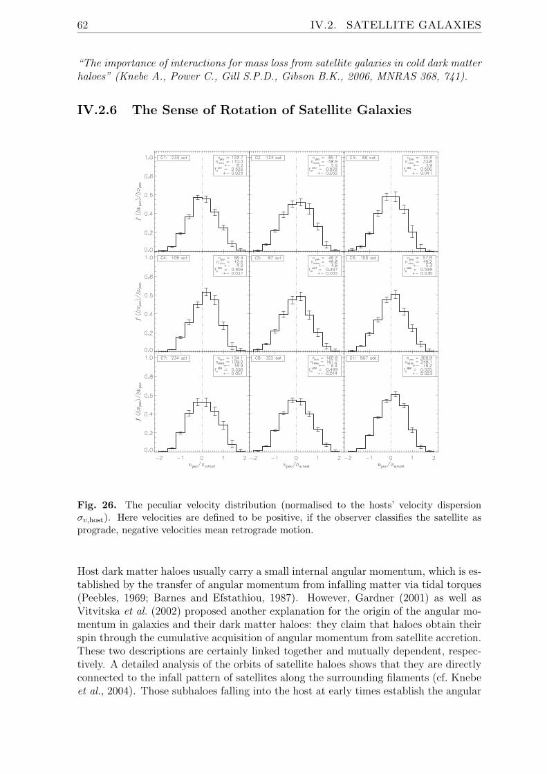
62 IV.2. SATELLITE GALAXIES
“The importance of interactions for mass loss from satellite galaxies in cold dark matterhaloes” (Knebe A., Power C., Gill S.P.D., Gibson B.K., 2006, MNRAS 368, 741).
IV.2.6 The Sense of Rotation of Satellite Galaxies
Fig. 26. The peculiar velocity distribution (normalised to the hosts’ velocity dispersionσv,host). Here velocities are defined to be positive, if the observer classifies the satellite asprograde, negative velocities mean retrograde motion.
Host dark matter haloes usually carry a small internal angular momentum, which is es-tablished by the transfer of angular momentum from infalling matter via tidal torques(Peebles, 1969; Barnes and Efstathiou, 1987). However, Gardner (2001) as well asVitvitska et al. (2002) proposed another explanation for the origin of the angular mo-mentum in galaxies and their dark matter haloes: they claim that haloes obtain theirspin through the cumulative acquisition of angular momentum from satellite accretion.These two descriptions are certainly linked together and mutually dependent, respec-tively. A detailed analysis of the orbits of satellite haloes shows that they are directlyconnected to the infall pattern of satellites along the surrounding filaments (cf. Knebeet al., 2004). Those subhaloes falling into the host at early times establish the angular

IV.3. DEBRIS FROM SATELLITE GALAXIES 63
momentum of the inner regions of the primary halo (cf. Vitvitska et al., 2002) andare channelled into the host along the same direction as those merging at later times.This leads to the speculation that satellites are preferentially co-rotating with the host,which is going to be investigated in Fig. 26.In Fig. 26 we present the results for the (differential) peculiar velocity distribution ofsubhaloes when viewed in 2D projection. We used one hundred random lines of sightand the velocities are normalised by the hosts’ velocity dispersion. All satellites to theleft of the vertical dash-dotted “zero” line have been classified as retrograde while allsatellites to the right are observed to be prograde. In addition, the mean number ofprograde and retrograde orbits (along with the 1σ deviation) is given for every host haloin the upper right corner of every panel. We get a mean observed prograde fraction of53.3% (±3.3%). The individual observed prograde fractions f
obsp for each dark matter
host are given in the inset panels of the respective plot of Fig. 26.Despite the weakness of the signal this is a new prediction of CDM structure formationthat can be verified observationally.
This work has been published as “The sense of rotation of subhaloes in cosmologicaldark matter haloes” (Warnick K., Knebe A., 2006, MNRAS 369, 1209).
IV.3 Debris from Satellite Galaxies
The tidal disruption of satellite galaxies is characteristic of the hierarchical mergingscenario. As a satellite galaxy orbits within the gravitational potential of its moremassive host, it is subject to a tidal field that may vary both in space and time. Thegravitational force acting on the satellite strips a stream of tidal debris from it, andin some cases tidal forces may be sufficient to lead to the complete disruption of thesystem. This tidal debris tends to form two distinct arms – a leading arm ahead of thesatellite and a trailing arm following the satellite.Observationally, large scale surveys have uncovered strong evidence for several tidalsteams around the Milky Way (see e.g. Belokurov et al., 2006; Grillmair, 2006; Powellet al., 2006, for recent observations). The well-known Magellanic stream is an exampleof a gaseous stream, arising from the tidal interaction of the Magellanic Clouds with ourGalaxy (e.g. Bekki and Chiba, 2005; Mastropietro et al., 2005; Connors et al., 2006).The tidal stream associated with the Sagittarius dwarf (Ibata et al., 1994) has beenstudied extensively (e.g. Johnston et al., 1995; Helmi and White, 2001; Majewski et al.,2003; Martınez-Delgado et al., 2004; Johnston et al., 2005, and many others), as hasthe Monoceros stream (Newberg et al., 2002; Yanny et al., 2003). Further, Ibata et al.(2001) have found evidence for a giant stream around M31, while deep photometricobservations by Brown et al. (2006) suggest that this tidal stream and the spheroid ofM31 have similar properties and hence may have a common origin. And even beyondour Local Group, Pohlen et al. (2004) and Wehner et al. (2006) have found evidence fortidal features around a number of distant galaxies, while the recent study of Corteseet al. (2007) has uncovered evidence for the tidal stripping of material from a spiralgalaxy that is in the process of disruption in the galaxy cluster Abell 2667.While previous studies of individual satellites disrupting in analytical host potentialsvia means of controlled N -body experiments hinted at simple and direct links between,for instance, flattening of the host and dispersion of the debris field (e.g., Ibata et al.,

64 IV.3. DEBRIS FROM SATELLITE GALAXIES
2003; Helmi, 2004; Penarrubia et al., 2006), the situation is vastly more complicated in“live” host haloes. Already Penarrubia et al. (2006) pointed out that there is only hopeto recover present-day properties of the host due to the adiabtic response of the streamto changes in the host potential, we actually go one step further: even the current stateof the host will be difficult to obtain given the complexity of interactions responsiblefor the emergence of derbris fields. There are multiple processes driving these effectsand so while we note tentative correlations, we require further simulations to help usunderstand what is happening. This will represent the focus of the following Sections.
IV.3.1 Mapping Substructures
Fig. 27. The distribution of satellite particles in the E−L plane for one of the cluster sizedhost haloes. The left panel shows the distributions at the time the respective satellite galaxyenters the virial radius of the host whereas the right panel presents the distributions at z = 0.Different colours represent particles of different satellites.
We present in Fig. 27 the evolution for eight different (tidally disrupting) satellitesin the so-called integrals-of-motions space, i.e. energy E vs. angular momentum L.Each satellite is represented by an individual colour. The satellites shown in Fig. 27are all taken from a self-consistent cosmological simulation of a galaxy cluster of massM ≈ 1014
h−1
M⊙ and represent a fair sample of all available satellites, i.e. their massescover a range from from M ∼ 5 × 10¹⁰
h−1
M⊙ to M ∼ 4 × 10¹²h−1
M⊙ and they areon different orbits. The left panel of Fig. 27 shows the distributions at the time therespective satellite enters the virial radius of the host, whereas the right panel displaysthe distributions at z = 0.Fig. 27 allows us to gauge the “drift” of satellites in integral-space. We note that,compared to Fig. 4 of Helmi and de Zeeuw (2000), the integrals-of-motion are hardlyconserved in our “live” model, neither for high nor low mass streamers. The distribu-tions rather show a large scatter, and have been significantly “re-shaped” over time. Inaddition, the mean values of E and L are also moved after the evolution. For instance,the “red” satellite drifts in time over to the initial position of the “cyan” satellite.
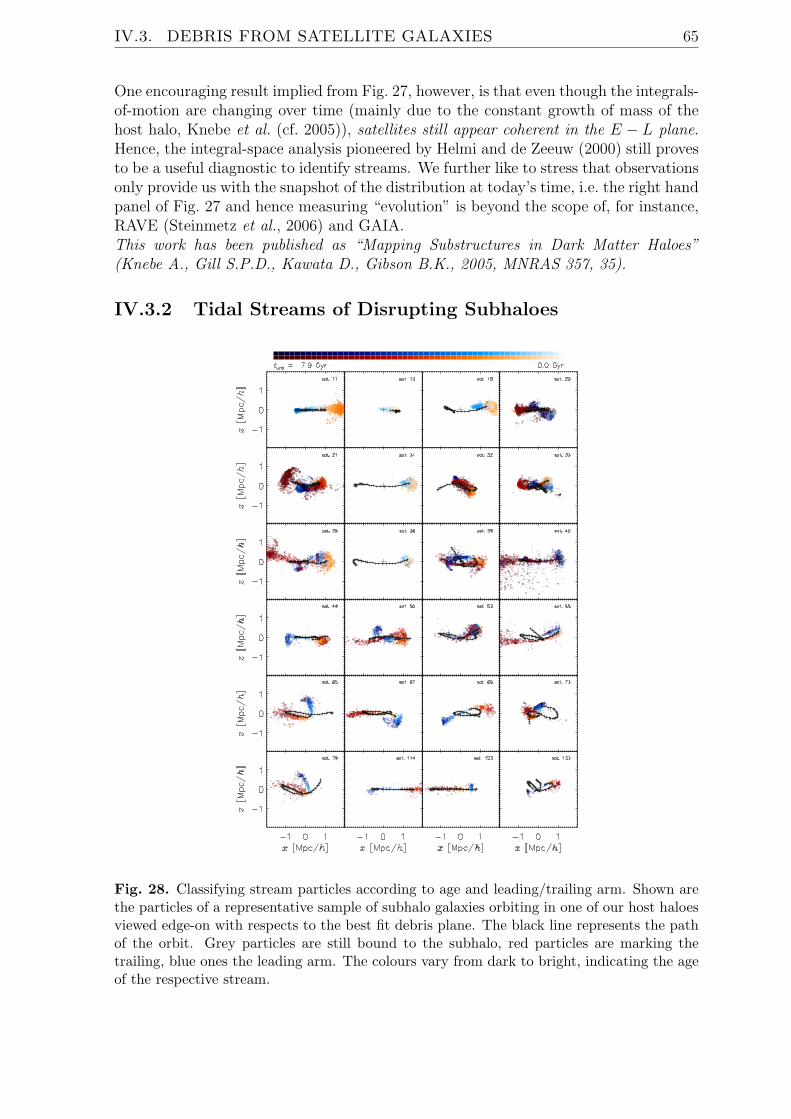
IV.3. DEBRIS FROM SATELLITE GALAXIES 65
One encouraging result implied from Fig. 27, however, is that even though the integrals-of-motion are changing over time (mainly due to the constant growth of mass of thehost halo, Knebe et al. (cf. 2005)), satellites still appear coherent in the E − L plane.Hence, the integral-space analysis pioneered by Helmi and de Zeeuw (2000) still provesto be a useful diagnostic to identify streams. We further like to stress that observationsonly provide us with the snapshot of the distribution at today’s time, i.e. the right handpanel of Fig. 27 and hence measuring “evolution” is beyond the scope of, for instance,RAVE (Steinmetz et al., 2006) and GAIA.This work has been published as “Mapping Substructures in Dark Matter Haloes”(Knebe A., Gill S.P.D., Kawata D., Gibson B.K., 2005, MNRAS 357, 35).
IV.3.2 Tidal Streams of Disrupting Subhaloes
Fig. 28. Classifying stream particles according to age and leading/trailing arm. Shown arethe particles of a representative sample of subhalo galaxies orbiting in one of our host haloesviewed edge-on with respects to the best fit debris plane. The black line represents the pathof the orbit. Grey particles are still bound to the subhalo, red particles are marking thetrailing, blue ones the leading arm. The colours vary from dark to bright, indicating the ageof the respective stream.

66 IV.3. DEBRIS FROM SATELLITE GALAXIES
In order to study leading and trailing debris arms we devised an automated methodto identify (and separate) these two arms and hence get a handle on their combinedas well as individual properties. A number of examples are given in Fig. 28 where weshow the orbits of a sample of satellites (crosses) and their respective debris fields. Thisfigure nicely demonstrates how well our method for tracking debris fields works andwe will now present one particular result. The particulars of this method are given inWarnick et al. (2008).
Fig. 29. The deviation of debris particles from the best fitting debris plane (normalised tothe virial radius of the respective host) as a function of infall mass for subhaloes with at leastone orbit. Backsplash subhaloes are marked with grey asterisks and the median values of thedistributions are shown in the lower right corners.
Our analysis of the tidal arms reveals that there is a relation between the scatter ofstream particles about the best-fit debris plane and the infall mass of the progenitorsubhalo. This allows us to reconstruct the infall mass from the spread of its tidal debrisin space: for Fig. 29 we fit a plane to the detected debris field and then determine thedeviation of the debris field from this best-fit plane and plot it against the original infallmass of the satellite (prior to disruption). We observe a correlation between infall massand debris deviation. Thus, by measuring the deviation of debris from the debris plane

IV.3. DEBRIS FROM SATELLITE GALAXIES 67
itself, it is possible for an observer to predict the most probable mass of the subhalo itoriginates from.This work has been published as “Tidal Streams of Disrupting Subhaloes in CosmologicalDark Matter Haloes” (Warnick K., Knebe A., Power C.B., 2008, MNRAS 385, 1859).


Part V
Conclusions & Outlook

70 V.1. CONCLUSIONS
V.1 Conclusions
During the past thirty years, numerical simulations of cosmic structure formation havebecome a powerful theoretical tool to accompany, interpret, and sometimes to leadcosmological observations. We presented a (more or less) thorough introduction intothis exciting discipline of “Computational Cosmology”. After a primer on the technicaldetails and numerical methods (Section II) simulations have been presented that lookedinto the differences between the standard ΛCDM model and alternative cosmologies(Section III) as well as an in-depth study of the dynamics and disruption of satellitegalaxies – the buildung blocks of cosmic structures (Section IV).In each of these sub-categories we can draw individual conclusions to be summarizedbelow.
Numerical Simulations We presented a novel solver for the integration of theequations-of-motion of dark matter particles under their mutual gravity as describedby Poisson’s equation. This solver is based upon arbitrarily shaped adaptive meshesand hence automatically adapts to the problem at hand. We further highlighted thedifferences to other codes in the field that utilize tree-structures to increase the com-putational speed for obtaining the relevant forces via direct summation.However, performing the simulation is only the first step in the study of cosmic struc-ture formation by means of computer simulations. One also needs to identify objects(galaxies, galaxy cluster, filaments, etc.) in them to be able to compare the resultsagainst observations. To this extent we also developed a new “halo finder” that isessentially parameter free. Both these codes (i.e. the simulation code MLAPM and thehalo finder MHF) have been made publically available to the community and our mainachievements/results can be summarized as follows.
• We developed an adaptive mesh gravity solver for cosmology.
• We developed a novel halo finder to be used with such simulations.
• Despite the diversity in numerical methods most of the codes used to simulatestructure formation agree with each other.
• Each method though has its strengths and weaknesses and we showed that, forinstance, two-body scattering is more prominent in tree-codes than in adaptive-mesh-refinement codes.
Alternative Cosmologies We tested whether we can solve to so-called “CDM cri-sis”, considering even the most extreme alternatives to dark matter (i.e. modifiedNewtonian dynamics (MOND), Milgrom (1983)). While most of the suggested solu-tions are (minor) modifications to the cold dark matter paradigm and include warmdark matter as well as effects from non-standard inflationary periods, MOND abandonsthe need for dark matter completely by adjusting the law of gravity. The main resultsfrom these studies can be summarized as follows.
• None of the studied alternatives is capable of simultaneously rectifying all short-comings of CDM.
• Warm dark matter greatly reduces the number of subhaloes.

V.1. CONCLUSIONS 71
• Warm dark matter haloes have lower concentrations.
• The likelihood of high-speed encounters akin to the “Bullet” cluster is greater inWDM than in CDM.
• Non-standard inflationary theories may lead to (bumpy) features in the powerspectrum of primordial density fluctuations and such “bumps” may mock differentcosmologies.
• MONDian cosmological simulations show that it is in fact possible to arrive at auniverse akin to the observed one with a different temporal evolution though.
Despite our efforts to solve the “CDM crisis” by merely tweaking the properties of darkmatter we belive that only when all the governing physics (dark matter and gas) isincluded in the theoretical modeling we will have a fair chance of understanding howgalaxies formed and evolved and will possibly resolve the CDM crisis. This refers tothe fact that our simulations are pure dark matter simulations whereas it is ratherobvious that on those scales for which the CDM crisis is apparant the physics of gasescan and should not be neglected. This last point is the main driver for further codedevelopment to be elaborated upon in the Outlook below.
Near-Field Cosmology Within the hierarchical structure formation scenario in-duced by cold dark matter the smallest entities, i.e. satellite galaxies, are the buildingblocks of all larger structures. It therefore appears mandatory to study their formation,evolution and tidal disruption in greater detail. Only recently it became possible toaddress this task not only observationally but also computationally. And as it combinesour knowledge of (large-scale) cosmology and small scale structures it has been dubbed“Near-Field Cosmology” (Freeman and Bland-Hawthorn, 2002). Utilizing a large suiteof (dark matter only) simulations of individual halos we explored the dynamics ofsubhaloes in great detail. The main results obtained are as follows.
• Subhaloes are radially aligned, i.e. their major axis points towards the centre ofthe host halo they orbit in.
• Subhaloes are anisotropically distributed, i.e. they are preferentially found alongthe major axis of their host halo.
• Subhaloes tend to be on orbits co-rotating with their host.
• Satellite-satellite interactions can lead to significant contributions to mass loss.
• Tidal debris fields from disrupting satellite galaxies are a powerful tool for study-ing the formation history of their host halos.
• We found a correlation between properties of the debris field and the intial mass(and orbital eccentricity) of the satellite.
• We developed a technique to separate the leading and trailing debris arm.
• Even in “live” host halos debris fields can be identified as coherent structures inthe integrals-of-motion space.

72 V.2. OUTLOOK
• However, the relation between host and debris properties is more complex thanderived from controlled experiments of individual satellites disrupting in analyt-ical (static) host potentials: we found little correlation of debris fields and hosthalo properties.
V.2 Outlook
Amongst many of the unanswered and open questions that emerged during the investi-gation of cosmic structure formation by means of numerical simulation that could onlybe in part presented in this thesis, we like to draw the attention to a small subset ofthe problems planned to be addressed in the near future.
The subhalo-satellite galaxy connection For the purposes of the studies pre-sented in this thesis, we treated “substructure haloes” (or subhaloes) and “satellitegalaxies” as interchangeable. However, the correspondence between dark matter sub-structures and luminous satellite galaxies is not a straightforward one. And despitegreat advances in refining numerical techniques allowing for an ever-increasing reso-lution of the problem under investigation, the implementation of more complicatedphysics such as gas physics significantly raises the complexity and hence degrades theresolution again. Therefore, complementary to modelling baryonic processes via numer-ical integration of the hydrodynamics equations we plan to engage in the discipline of“semi-analytical galaxy formation”. Such a method combines our current understand-ing of galaxy formation with the predictions from dissipationless CDM simulations suchas the ones presented in this thesis. It utilizes the merger trees of dark matter haloesfound in the simulations and adds analytical prescriptions for galaxy formation. Theparameters of these recipes are gauged by observations of galaxies in the local Universe.This technique has recently been extremely successfull in explaining the intriguingresult that all satellites of the Milky Way have the same mass interior to 300 parsec, i.e.M ≈ 107
M⊙ while spanning almost four orders of magnitude in luminosity (Strigariet al., 2008; Li et al., 2008b; Maccio’ et al., 2008). However, at present, it remainsunclear whether the luminosity function of the satellites of the Milky Way and theirpeculiar spatial distribution are unique to the Galaxy, or whether these are genericfeatures that arise during the formation of a typical galaxy. For instance, we foundthat there exists a prominent population of “backsplash” subhaloes outside the (virial)radius of even galactic host haloes. Therefore, we should be able to detect theseobjects also about the Milky Way. But to allow for a comparison with obsverationpredictions for their luminosities and/or morphologies are required, too. Therefore,the future plan is to couple the semi-analytical code GalICS (Hatton et al., 2003) toour suite of dark matter haloes (cf. Section IV) and derive observable properties for thesatellite galaxy population orbiting within them. We plan to address the question ofthe (putative) backsplash population and their possible relation to the rather peculiarspatial distribution of satellites on a so-called “disk of satellites” (Metz et al., 2007,2008). We further like to know what actually determines the number of Milky Waysatellites and what shapes their luminosity function.
Galaxies at high-redshift Besides of the discrepancies between simulations of hier-archical structure formation and observations at low redshift (cf. Section III) there also

V.2. OUTLOOK 73
appear to be problems related to our understanding of structure formation at high red-shift. There is a divergence between the predictions of analytic models and the resultsof computer simulations that follow the formation of the first objects in our Universe:while Jenkins et al. (2001) showed that the mass function of dark matter haloes ap-pears to be universal, the recent years have seen a number of studies indicating thatthis universality actually breaks down in the high-redshift universe (Springel et al.,2005; Reed et al., 2005; Heitmann et al., 2006; Betancort-Rijo and Montero-Dorta,2006; Reed et al., 2007). However, can we be certain to actually model and simulatethe mass function at those high-redshifts accurately? While a lot of efforts have beendirected towards modeling haloes as accurately as possible at low redshifts, high red-shift simulations, however, suffer from their own set of systematic issues as quantifiedby Lukic et al. (2007). But as haloes forming at redshifts around z ≈ 15 − 20 willhost the first galaxies and stars that (presumably) re-ionized the Universe, a preciseand quantitative understanding of those objects (and their abundance) is crucial for acomprehension of the subsequent structure formation. Further, the properties of thoseearly objects can significantly differ from the particulars of their present day counter-parts (Cohn and White, 2008; Knebe and Power, 2008) further pointing towards thenecessity to study them in greater detail.In that regards we plan to investigate the abundance of objects at redshifts z ≥ 10 byutilizing extremely high-resolution cosmological simulations of hierarchical structureformation taking into account the criteria set by Lukic et al. (2007). This then allowsus to establish the mass function of high redshift haloes. We shall further apply thetechnique of semi-analytical galaxy formation alluded to above to make predictionsthat can be tested by the next generation of 21cm missions such as LOFAR and theSKA that will observationally probe that redshift regime.
Cosmological Magneto-Hydrodynamics Magnetic fields play an important rolein almost all astrophysical phenomena including star formation. But due to the diffi-culty in analytic modeling magnetic fields are still poorly understood; numerical sim-ulation again is the major tool for studying their effects and impact.When it comes to the local Universe, it has been well established that there arewidespread magnetic fields in the intracluster medium (e.g. Carilli and Taylor, 2002;Govoni, 2006, for a recent review). There has also been tantalizing evidence for mag-netic fields in the wider intergalactic medium. The origin of these large-scale magneticfields is still unknown. Furthermore, it is presently mostly unknown whether thesemagnetic fields have played an important role or not in systems ranging from large-scale structure formation over galaxy clusters to cluster core regions and to galaxyformation itself. There have only been a few studies aiming at investigating the roleof magnetic fields in the intracluster and intergalactic medium to date (e.g. Ryu et al.,1998; Dolag et al., 2002, 2005; Bruggen et al., 2005; Li et al., 2008a; Xu et al., 2008),most of them not in a cosmological context.With regards to the high-redshift Universe, preliminary investigations of the relevanceof magnetic fields for cosmic structure formation scenarios reveal that their effectscannot be neglected (Sethi et al., 2008). The presence of magnetic fields in the earlyUniverse can significantly change the standard history of star formation and they canfurther seed early formation of structures (Sethi and Subramanian, 2005).We therefore went one step further than simply adding gas physics to our simulationcode described in Section II.6; we added the equations of magneto-hydrodynamics in su-

74 V.2. OUTLOOK
percomoving coordinates to MLAPM that are being solved by a conservative, divergence-free Godunov-type central scheme (Ziegler, 2005). And first test runs indicate thatthe presence of magnetic fields in the early universe will have an impact upon cosmicstructure formation. We are currently in the process of confirming this finding withbetter resolved simulations and differing initial magnetic field configurations.
Cosmological Modified Newtonian Dynamics We just fininshed developing anovel solver for the analogue to Poisson’s equation in the framework of modified New-tonian dynamics (MOND)
∇ ·
µ
|∇ΦM |
a2g0
∇ΦM
=4πG
a(ρ− ρ) . (V.1)
This equation is (in contrast to the Newtonian Poisson’s equation) highly non-linearand hence standard codes based upon tree structures and/or FFT’s in general are notapplicable to solve it; one needs to defer to multi-grid relaxation techniques. We willutilize this new code to revisit the issue of cosmic structure formation under MOND.14
And first steps in that direction show that, for instance, the probability of high-speedencounters between galaxy clusters (as, for instance, observed in the “Bullet cluster”,Markevitch (2006)) are more likely in MOND than in dark matter scenarios. Never-theless, structure formation in a MONDian universe appears to be more rapid withless structures at high redshift – possibly in contradiction to observations. We hope toclarify this and either rule out or confirm the venturesome theory of MOND.
14Note that for the study presented in Section III.4 we did not solve the MONDian Poisson’sequation but rather modified the Newtonian potential according to a prescription based upon variousassumptions to account for the affects of MOND.

Bibliography
Aarseth, S. J. (1963). Dynamical evolution of clusters of galaxies, I. MNRAS, 126,223–+.
Agertz, O., Moore, B., Stadel, J., Potter, D., Miniati, F., Read, J., Mayer, L.,Gawryszczak, A., Kravtsov, A., Nordlund, A., Pearce, F., Quilis, V., Rudd, D.,Springel, V., Stone, J., Tasker, E., Teyssier, R., Wadsley, J., and Walder, R. (2007).Fundamental differences between SPH and grid methods. MNRAS, 380, 963–978.
Agustsson, I. and Brainerd, T. G. (2006). The Orientation of Satellite Galaxies: Evi-dence of Elongation in the Direction of the Host. ApJ, 644, L25–L28.
Akerib, D. S., Armel-Funkhouser, M. S., Attisha, M. J., Bailey, C. N., Baudis, L.,Bauer, D. A., Brink, P. L., Bunker, R., Cabrera, B., Caldwell, D. O., Chang, C. L.,Crisler, M. B., Cushman, P., Daal, M., Dixon, R., Dragowsky, M. R., Driscoll, D. D.,Duong, L., Ferril, R., Filippini, J., Gaitskell, R. J., Hennings-Yeomans, R., Holm-gren, D., Huber, M. E., Kamat, S., Lu, A., Mahapatra, R., Mandic, V., Martinis,J. M., Meunier, P., Mirabolfathi, N., Nelson, H., Nelson, R., Ogburn, R. W., Per-era, T. A., Issac, M. C., Ramberg, E., Rau, W., Reisetter, A., Ross, R. R., Saab,T., Sadoulet, B., Sander, J., Savage, C., Schnee, R. W., Seitz, D. N., Serfass, B.,Sundqvist, K. M., Thompson, J.-P. F., Wang, G., Yellin, S., and Young, B. A. (2005).Exclusion limits on the WIMP-nucleon cross section from the first run of the Cryo-genic Dark Matter Search in the Soudan Underground Laboratory. Phys. Rev. D,72(5), 052009–+.
Allgood, B., Flores, R. A., Primack, J. R., Kravtsov, A. V., Wechsler, R. H., Fal-tenbacher, A., and Bullock, J. S. (2006). The shape of dark matter haloes: depen-dence on mass, redshift, radius and formation. MNRAS, 367, 1781–1796.
Avila-Reese, V., Colın, P., Valenzuela, O., D’Onghia, E., and Firmani, C. (2001).Formation and Structure of Halos in a Warm Dark Matter Cosmology. ApJ, 559,516–530.
Baertschiger, T., Joyce, M., and Sylos Labini, F. (2002). Power-Law Correlation andDiscreteness in Cosmological N-Body Simulations. ApJ, 581, L63–L66.
Bahcall, N. A., Fan, X., and Cen, R. (1997). Constraining Omega with Cluster Evolu-tion. ApJ, 485, L53+.
Bahcall, N. A., Ostriker, J. P., Perlmutter, S., and Steinhardt, P. J. (1999). The CosmicTriangle: Revealing the State of the Universe. Science, 284, 1481–+.

76 BIBLIOGRAPHY
Bailin, J. and Steinmetz, M. (2005). Internal and External Alignment of the Shapesand Angular Momenta of ΛCDM Halos. ApJ, 627, 647–665.
Bardeen, J. M., Bond, J. R., Kaiser, N., and Szalay, A. S. (1986). The statistics ofpeaks of Gaussian random fields. ApJ, 304, 15–61.
Barnes, J. and Efstathiou, G. (1987). Angular momentum from tidal torques. ApJ,319, 575–600.
Barnes, J. and Hut, P. (1986). A Hierarchical O(NlogN) Force-Calculation Algorithm.Nature, 324, 446–449.
Barriga, J., Gaztanaga, E., Santos, M. G., and Sarkar, S. (2001). Evidence for an in-flationary phase transition from the LSS and CMB anisotropy data. Nuclear PhysicsB Proceedings Supplements , 95, 66–69.
Begeman, K. G., Broeils, A. H., and Sanders, R. H. (1991). Extended rotation curvesof spiral galaxies - Dark haloes and modified dynamics. MNRAS, 249, 523–537.
Bekenstein, J. and Milgrom, M. (1984). Does the missing mass problem signal thebreakdown of Newtonian gravity? ApJ, 286, 7–14.
Bekki, K. and Chiba, M. (2005). Formation and evolution of the Magellanic Clouds- I. Origin of structural, kinematic and chemical properties of the Large MagellanicCloud. MNRAS, 356, 680–702.
Belokurov, V., Zucker, D. B., Evans, N. W., Gilmore, G., Vidrih, S., Bramich, D. M.,Newberg, H. J., Wyse, R. F. G., Irwin, M. J., Fellhauer, M., Hewett, P. C., Walton,N. A., Wilkinson, M. I., Cole, N., Yanny, B., Rockosi, C. M., Beers, T. C., Bell,E. F., Brinkmann, J., Ivezic, Z., and Lupton, R. (2006). The Field of Streams:Sagittarius and Its Siblings. ApJ, 642, L137–L140.
Bento, M. C., Bertolami, O., Rosenfeld, R., and Teodoro, L. (2000). Self-interactingdark matter and the Higgs boson. Phys. Rev. D, 62(4), 041302–+.
Bertschinger, E. and Gelb, J. M. (1991). Cosmological N-body simulations. Computersin Physics , 5, 164–175.
Betancort-Rijo, J. E. and Montero-Dorta, A. D. (2006). Understanding the CosmicMass Function High-Mass Behavior. ApJ, 650, L95–L98.
Bett, P., Eke, V., Frenk, C. S., Jenkins, A., Helly, J., and Navarro, J. (2007). Thespin and shape of dark matter haloes in the Millennium simulation of a Λ cold darkmatter universe. MNRAS, 376, 215–232.
Binney, J. and Knebe, A. (2002). Two-body relaxation in cosmological simulations.MNRAS, 333, 378–382.
Bode, P. and Ostriker, J. P. (2003). Tree Particle-Mesh: An Adaptive, Efficient, andParallel Code for Collisionless Cosmological Simulation. ApJS, 145, 1–13.
Bode, P., Ostriker, J. P., and Turok, N. (2001). Halo Formation in Warm Dark MatterModels. ApJ, 556, 93–107.

BIBLIOGRAPHY 77
Bond, J. R. and Szalay, A. S. (1983). The collisionless damping of density fluctuationsin an expanding universe. ApJ, 274, 443–468.
Brandt, A. (1977). Multi-Level Adaptive Solutions to Boundary-Value Problems. Math.of Comp., 31, 333–390.
Brown, T. M., Smith, E., Guhathakurta, P., Rich, R. M., Ferguson, H. C., Renzini,A., Sweigart, A. V., and Kimble, R. A. (2006). Deep Photometry of AndromedaReveals Striking Similarities in the Tidal Stream and Spheroid Populations. ApJ,636, L89–L92.
Bruggen, M., Ruszkowski, M., Simionescu, A., Hoeft, M., and Dalla Vecchia, C. (2005).Simulations of Magnetic Fields in Filaments. ApJ, 631, L21–L24.
Bryan, G. L. and Norman, M. L. (1998). Statistical Properties of X-Ray Clusters:Analytic and Numerical Comparisons. ApJ, 495, 80–+.
Buchert, T. and Domınguez, A. (2005). Adhesive gravitational clustering. A&A, 438,443–460.
Bullock, J. S. (2001). Tilted CDM versus WDM in the Subgalactic Scuffle. ArXivAstrophysics e-prints (0111005).
Bullock, J. S., Kolatt, T. S., Sigad, Y., Somerville, R. S., Kravtsov, A. V., Klypin,A. A., Primack, J. R., and Dekel, A. (2001). Profiles of dark haloes: evolution,scatter and environment. MNRAS, 321, 559–575.
Carilli, C. L. and Taylor, G. B. (2002). Cluster Magnetic Fields. ARA&A, 40, 319–348.
Chapman, S. and Cowling, T. G. (1991). The Mathematical Theory of Non-uniformGases . The Mathematical Theory of Non-uniform Gases, by Sydney Chapman andT. G. Cowling and Foreword by C. Cercignani, pp. 447. ISBN 052140844X. Cam-bridge, UK: Cambridge University Press, January 1991.
Chung, D. J. H., Kolb, E. W., Riotto, A., and Tkachev, I. I. (2000). Probing Planck-ian physics: Resonant production of particles during inflation and features in theprimordial power spectrum. Phys. Rev. D, 62(4), 043508–+.
Clowe, D., Gonzalez, A., and Markevitch, M. (2004). Weak-Lensing Mass Reconstruc-tion of the Interacting Cluster 1E 0657-558: Direct Evidence for the Existence ofDark Matter. ApJ, 604, 596–603.
Cohn, J. D. and White, M. (2008). Dark matter halo abundances, clustering andassembly histories at high redshift. MNRAS, 385, 2025–2033.
Colın, P., Avila-Reese, V., and Valenzuela, O. (2000). Substructure and Halo DensityProfiles in a Warm Dark Matter Cosmology. ApJ, 542, 622–630.
Connors, T. W., Kawata, D., and Gibson, B. K. (2006). N-body simulations of theMagellanic stream. MNRAS, 371, 108–120.

78 BIBLIOGRAPHY
Cortese, L., Marcillac, D., Richard, J., Bravo-Alfaro, H., Kneib, J.-P., Rieke, G., Cov-one, G., Egami, E., Rigby, J., Czoske, O., and Davies, J. (2007). The strong trans-formation of spiral galaxies infalling into massive clusters at z ˜ 0.2. MNRAS, 376,157–172.
Couchman, H. M. P. (1991). Mesh-refined P3M - A fast adaptive N-body algorithm.ApJ, 368, L23–L26.
Croft, R. A. C., Weinberg, D. H., Bolte, M., Burles, S., Hernquist, L., Katz, N.,Kirkman, D., and Tytler, D. (2002). Toward a Precise Measurement of MatterClustering: Lyα Forest Data at Redshifts 2-4. ApJ, 581, 20–52.
Dahle, H., Pedersen, K., Lilje, P. B., Maddox, S. J., and Kaiser, N. (2003). WeakGravitational Lensing by a Sample of X-Ray-luminous Clusters of Galaxies. III.Serendipitous Weak Lensing Detections of Dark and Luminous Mass Concentrations.ApJ, 591, 662–676.
Dalal, N. and Kochanek, C. S. (2002). Direct Detection of Cold Dark Matter Substruc-ture. ApJ, 572, 25–33.
Davis, M., Efstathiou, G., Frenk, C. S., and White, S. D. M. (1985). The evolutionof large-scale structure in a universe dominated by cold dark matter. ApJ, 292,371–394.
Dehnen, W. (2001). Towards optimal softening in three-dimensional N-body codes - I.Minimizing the force error. MNRAS, 324, 273–291.
Dicke, R. H., Peebles, P. J. E., Roll, P. G., and Wilkinson, D. T. (1965). CosmicBlack-Body Radiation. ApJ, 142, 414–419.
Diemand, J., Moore, B., Stadel, J., and Kazantzidis, S. (2004). Two-body relaxationin cold dark matter simulations. MNRAS, 348, 977–986.
Diemand, J., Moore, B., and Stadel, J. (2005). Earth-mass dark-matter haloes as thefirst structures in the early Universe. Nature, 433, 389–391.
Dolag, K., Bartelmann, M., and Lesch, H. (2002). Evolution and structure of magneticfields in simulated galaxy clusters. A&A, 387, 383–395.
Dolag, K., Grasso, D., Springel, V., and Trachev, I. (2005). Simulating the MagneticField in the Local Supercluster. In L. O. Sjouwerman and K. K. Dyer, editors,X-Ray and Radio Connections (eds. L.O. Sjouwerman and K.K Dyer) Publishedelectronically by NRAO, http://www.aoc.nrao.edu/events/xraydio Held 3-6 February2004 in Santa Fe, New Mexico, USA, (E8.10) 6 pages .
Domınguez, A. (2000). Hydrodynamic approach to the evolution of cosmological struc-tures. Phys. Rev. D, 62(10), 103501–+.
Doroshkevich, A. G., Sunyaev, R. A., and Zeldovich, I. B. (1974). The formationof galaxies in Friedmannian universes. In M. S. Longair, editor, Confrontation ofCosmological Theories with Observational Data, volume 63 of IAU Symposium, pages213–225.

BIBLIOGRAPHY 79
Efstathiou, G., Davis, M., White, S. D. M., and Frenk, C. S. (1985). Numericaltechniques for large cosmological N-body simulations. ApJS, 57, 241–260.
Eisenstein, D. J. and Hu, W. (1998). Baryonic Features in the Matter Transfer Func-tion. ApJ, 496, 605–+.
El-Zant, A. A. (2006). Two-body relaxation in simulated cosmological haloes. MNRAS,370, 1247–1256.
Faltenbacher, A., Li, C., Mao, S., van den Bosch, F. C., Yang, X., Jing, Y. P., Pasquali,A., and Mo, H. J. (2007). Three Different Types of Galaxy Alignment within DarkMatter Halos. ApJ, 662, L71–L74.
Faltenbacher, A., Jing, Y. P., Li, C., Mao, S., Mo, H. J., Pasquali, A., and van denBosch, F. C. (2008). Spatial and Kinematic Alignments between Central and SatelliteHalos. ApJ, 675, 146–155.
Freeman, K. and Bland-Hawthorn, J. (2002). The New Galaxy: Signatures of ItsFormation. ARA&A, 40, 487–537.
Frenk, C. S., White, S. D. M., Davis, M., and Efstathiou, G. (1988). The formation ofdark halos in a universe dominated by cold dark matter. ApJ, 327, 507–525.
Frenk, C. S., White, S. D. M., Bode, P., Bond, J. R., Bryan, G. L., Cen, R., Couchman,H. M. P., Evrard, A. E., Gnedin, N., Jenkins, A., Khokhlov, A. M., Klypin, A.,Navarro, J. F., Norman, M. L., Ostriker, J. P., Owen, J. M., Pearce, F. R., Pen, U.-L., Steinmetz, M., Thomas, P. A., Villumsen, J. V., Wadsley, J. W., Warren, M. S.,Xu, G., and Yepes, G. (1999). The Santa Barbara Cluster Comparison Project: AComparison of Cosmological Hydrodynamics Solutions. ApJ, 525, 554–582.
Gardiner, L. T. and Noguchi, M. (1996). N-body simulations of the Small MagellanicCloud and the Magellanic Stream. MNRAS, 278, 191–208.
Gardner, J. P. (2001). Dependence of Halo Properties on Interaction History, Environ-ment, and Cosmology. ApJ, 557, 616–625.
Gelb, J. M. and Bertschinger, E. (1994). Cold dark matter. 1: The formation of darkhalos. ApJ, 436, 467–490.
Gentile, G., Tonini, C., and Salucci, P. (2007). ΛCDM halo density profiles: where doactual halos converge to NFW ones? A&A, 467, 925–931.
Ghigna, S., Moore, B., Governato, F., Lake, G., Quinn, T., and Stadel, J. (1998). Darkmatter haloes within clusters. MNRAS, 300, 146–162.
Gill, S. P. D., Knebe, A., and Gibson, B. K. (2004a). The evolution of substructure -I. A new identification method. MNRAS, 351, 399–409.
Gill, S. P. D., Knebe, A., Gibson, B. K., and Dopita, M. A. (2004b). The evolution ofsubstructure - II. Linking dynamics to environment. MNRAS, 351, 410–422.
Gingold, R. A. and Monaghan, J. J. (1977). Smoothed particle hydrodynamics - Theoryand application to non-spherical stars. MNRAS, 181, 375–389.

80 BIBLIOGRAPHY
Gnedin, N. Y. (1995). Softened Lagrangian hydrodynamics for cosmology. ApJS, 97,231–257.
Goetz, M., Huchra, J. P., and Brandenberger, R. H. (1998). Group Identificationin N-Body Simulations: SKID and DENMAX Versus Friends-of-Friends. ArXivAstrophysics e-prints .
Gottlober, S. and Yepes, G. (2007). Shape, Spin, and Baryon Fraction of Clusters inthe MareNostrum Universe. ApJ, 664, 117–122.
Govoni, F. (2006). Observations of magnetic fields in regular and irregular clusters.Astronomische Nachrichten, 327, 539–+.
Grillmair, C. J. (2006). Substructure in Tidal Streams: Tributaries in the AnticenterStream. ApJ, 651, L29–L32.
Groth, E. J., Peebles, P. J. E., Seldner, M., and Soneira, R. M. (1977). The clusteringof galaxies. Scientific American, 237, 76–78.
Gunn, J. E. and Gott, J. R. I. (1972). On the Infall of Matter Into Clusters of Galaxiesand Some Effects on Their Evolution. ApJ, 176, 1–+.
Hannestad, S., Hansen, S. H., and Villante, F. L. (2001). Probing the power spectrumbend with recent cosmic microwave background data. Astroparticle Physics , 16,137–144.
Hatton, S., Devriendt, J. E. G., Ninin, S., Bouchet, F. R., Guiderdoni, B., and Vibert,D. (2003). GALICS- I. A hybrid N-body/semi-analytic model of hierarchical galaxyformation. MNRAS, 343, 75–106.
Hawley, D. L. and Peebles, P. J. E. (1975). Distribution of observed orientations ofgalaxies. AJ, 80, 477–491.
Hayashi, E. and White, S. D. M. (2006). How rare is the bullet cluster? MNRAS, 370,L38–L41.
Hayashi, E., Navarro, J. F., Taylor, J. E., Stadel, J., and Quinn, T. (2003). TheStructural Evolution of Substructure. ApJ, 584, 541–558.
Heitmann, K., Lukic, Z., Habib, S., and Ricker, P. M. (2006). Capturing Halos at HighRedshifts. ApJ, 642, L85–L88.
Heitmann, K., Lukic, Z., Fasel, P., Habib, S., Warren, M. S., White, M., Ahrens, J.,Ankeny, L., Armstrong, R., O’Shea, B., Ricker, P. M., Springel, V., Stadel, J., andTrac, H. (2007). The Cosmic Code Comparison Project. ArXiv e-prints , 706.
Helmi, A. (2004). Is the dark halo of our Galaxy spherical? MNRAS, 351, 643–648.
Helmi, A. and de Zeeuw, P. T. (2000). Mapping the substructure in the Galactic halowith the next generation of astrometric satellites. MNRAS, 319, 657–665.
Helmi, A. and White, S. D. M. (2001). Simple dynamical models of the Sagittariusdwarf galaxy. MNRAS, 323, 529–536.

BIBLIOGRAPHY 81
Hockney, R. W. and Eastwood, J. W. (1988). Computer simulation using particles .Bristol: Hilger, 1988.
Holmberg, E. (1969). A study of physical groups of galaxies. Arkiv for Astronomi , 5,305–343.
Hubble, E. and Humason, M. L. (1931). The Velocity-Distance Relation among Extra-Galactic Nebulae. ApJ, 74, 43–+.
Ibata, R., Irwin, M., Lewis, G., Ferguson, A. M. N., and Tanvir, N. (2001). A giantstream of metal-rich stars in the halo of the galaxy M31. Nature, 412, 49–52.
Ibata, R. A., Gilmore, G., and Irwin, M. J. (1994). A Dwarf Satellite Galaxy inSagittarius. Nature, 370, 194–+.
Ibata, R. A., Irwin, M. J., Lewis, G. F., Ferguson, A. M. N., and Tanvir, N. (2003).One ring to encompass them all: a giant stellar structure that surrounds the Galaxy.MNRAS, 340, L21–L27.
Icke, V. (1985). Distant encounters between disk galaxies and the origin of S 0 spirals.A&A, 144, 115–123.
Jenkins, A., Frenk, C. S., White, S. D. M., Colberg, J. M., Cole, S., Evrard, A. E.,Couchman, H. M. P., and Yoshida, N. (2001). The mass function of dark matterhaloes. MNRAS, 321, 372–384.
Johnston, K. V., Spergel, D. N., and Hernquist, L. (1995). The Disruption of theSagittarius Dwarf Galaxy. ApJ, 451, 598–+.
Johnston, K. V., Hernquist, L., and Bolte, M. (1996). Fossil Signatures of AncientAccretion Events in the Halo. ApJ, 465, 278–+.
Johnston, K. V., Law, D. R., and Majewski, S. R. (2005). A Two Micron All SkySurvey View of the Sagittarius Dwarf Galaxy. III. Constraints on the Flattening ofthe Galactic Halo. ApJ, 619, 800–806.
Kasun, S. F. and Evrard, A. E. (2005). Shapes and Alignments of Galaxy ClusterHalos. ApJ, 629, 781–790.
Klypin, A. and Holtzman, J. (1997). Particle-Mesh code for cosmological simulations.ArXiv Astrophysics e-prints .
Klypin, A., Gottlober, S., Kravtsov, A. V., and Khokhlov, A. M. (1999a). Galaxies inN-Body Simulations: Overcoming the Overmerging Problem. ApJ, 516, 530–551.
Klypin, A., Kravtsov, A. V., Valenzuela, O., and Prada, F. (1999b). Where Are theMissing Galactic Satellites? ApJ, 522, 82–92.
Klypin, A. A. and Shandarin, S. F. (1983). Three-dimensional numerical model of theformation of large-scale structure in the Universe. MNRAS, 204, 891–907.
Knebe, A. and Gibson, B. K. (2004). Galactic haloes in MONDian cosmological sim-ulations. MNRAS, 347, 1055–1064.

82 BIBLIOGRAPHY
Knebe, A. and Power, C. (2008). On the Correlation between Spin Parameter andHalo Mass. ApJ, 678, 621–626.
Knebe, A., Green, A., and Binney, J. (2001). Multi-level adaptive particle mesh(MLAPM): a c code for cosmological simulations. MNRAS, 325, 845–864.
Knebe, A., Devriendt, J. E. G., Mahmood, A., and Silk, J. (2002). Merger histories inwarm dark matter structure formation scenarios. MNRAS, 329, 813–828.
Knebe, A., Gill, S. P. D., Gibson, B. K., Lewis, G. F., Ibata, R. A., and Dopita, M. A.(2004). Anisotropy in the Distribution of Satellite Galaxy Orbits. ApJ, 603, 7–11.
Knebe, A., Gill, S. P. D., Kawata, D., and Gibson, B. K. (2005). Mapping substructuresin dark matter haloes. MNRAS, 357, L35–L39.
Knebe, A., Domınguez, A., and Domınguez-Tenreiro, R. (2006). Hydrodynamic ap-proach to the evolution of cosmic structures - II. Study of N-body simulations at z= 0. MNRAS, 371, 1959–1974.
Knebe, A., Draganova, N., Power, C., Yepes, G., Hoffman, Y., Gottlober, S., andGibson, B. K. (2008a). On the relation between the radial alignment of dark mattersubhaloes and host mass in cosmological simulations. MNRAS, 386, L52–L56.
Knebe, A., Yahagi, H., Kase, H., Lewis, G., and Gibson, B. K. (2008b). The radialalignment of dark matter subhalos: from simulations to observations. ArXiv e-prints ,805.
Komatsu, E., Dunkley, J., Nolta, M. R., Bennett, C. L., Gold, B., Hinshaw, G., Jarosik,N., Larson, D., Limon, M., Page, L., Spergel, D. N., Halpern, M., Hill, R. S., Kogut,A., Meyer, S. S., Tucker, G. S., Weiland, J. L., Wollack, E., and Wright, E. L.(2008). Five-Year Wilkinson Microwave Anisotropy Probe (WMAP) Observations:Cosmological Interpretation. ArXiv e-prints , 803.
Kravtsov, A. V., Klypin, A. A., and Khokhlov, A. M. (1997). Adaptive RefinementTree: A New High-Resolution N-Body Code for Cosmological Simulations. ApJS,111, 73–+.
Kravtsov, A. V., Gnedin, O. Y., and Klypin, A. A. (2004). The Tumultuous Lives ofGalactic Dwarfs and the Missing Satellites Problem. ApJ, 609, 482–497.
Kuhlen, M., Diemand, J., and Madau, P. (2007). The Shapes, Orientation, and Align-ment of Galactic Dark Matter Subhalos. ApJ, 671, 1135–1146.
Larson, R. B., Tinsley, B. M., and Caldwell, C. N. (1980). The evolution of diskgalaxies and the origin of S0 galaxies. ApJ, 237, 692–707.
Leeuwin, F., Combes, F., and Binney, J. (1993). N-body simulations with perturbationparticles. I - Method and tests. MNRAS, 262, 1013–1022.
Lesgourgues, J., Polarski, D., and Starobinsky, A. A. (1998). CDM models with a BSIstep-like primordial spectrum and a cosmological constant. MNRAS, 297, 769–776.

BIBLIOGRAPHY 83
Li, S., Li, H., and Cen, R. (2008a). CosmoMHD: A Cosmological Magnetohydrody-namics Code. ApJS, 174, 1–12.
Li, Y.-S., Helmi, A., De Lucia, G., and Stoehr, F. (2008b). On the common mass scaleof the Milky Way satellites. ArXiv e-prints .
Lin, D. N. C., Jones, B. F., and Klemola, A. R. (1995). The motion of the Magellanicclouds, origin of the Magellanic Stream, and the mass of the Milky Way. ApJ, 439,652–671.
Little, B., Knebe, A., and Islam, R. R. (2003). Warm dark matter versus bumpy powerspectra. MNRAS, 341, 617–622.
Lucy, L. B. (1977). A numerical approach to the testing of the fission hypothesis. AJ,82, 1013–1024.
Lukic, Z., Heitmann, K., Habib, S., Bashinsky, S., and Ricker, P. M. (2007). The HaloMass Function: High-Redshift Evolution and Universality. ApJ, 671, 1160–1181.
Maccio, A. V., Dutton, A. A., van den Bosch, F. C., Moore, B., Potter, D., and Stadel,J. (2007). Concentration, spin and shape of dark matter haloes: scatter and thedependence on mass and environment. MNRAS, 378, 55–71.
Maccio’, A. V., Kang, X., and Moore, B. (2008). Central mass and luminosity of MilkyWay satellites in the LCDM model. ArXiv e-prints .
Majewski, S. R., Skrutskie, M. F., Weinberg, M. D., and Ostheimer, J. C. (2003). ATwo Micron All Sky Survey View of the Sagittarius Dwarf Galaxy. I. Morphology ofthe Sagittarius Core and Tidal Arms. ApJ, 599, 1082–1115.
Markevitch, M. (2006). Chandra Observation of the Most Interesting Cluster in theUniverse. In A. Wilson, editor, The X-ray Universe 2005 , volume 604 of ESA SpecialPublication, pages 723–+.
Martin, J., Riazuelo, A., and Sakellariadou, M. (2000). Nonvacuum initial states forcosmological perturbations of quantum-mechanical origin. Phys. Rev. D, 61(8),083518–+.
Martınez-Delgado, D., Gomez-Flechoso, M. A., Aparicio, A., and Carrera, R. (2004).Tracing Out the Northern Tidal Stream of the Sagittarius Dwarf Spheroidal Galaxy.ApJ, 601, 242–259.
Mastropietro, C., Moore, B., Mayer, L., Wadsley, J., and Stadel, J. (2005). Thegravitational and hydrodynamical interaction between the Large Magellanic Cloudand the Galaxy. MNRAS, 363, 509–520.
McGaugh, S. S. and de Blok, W. J. G. (1998). Testing the Hypothesis of ModifiedDynamics with Low Surface Brightness Galaxies and Other Evidence. ApJ, 499,66–+.
McGaugh, S. S., de Blok, W. J. G., Schombert, J. M., Kuzio de Naray, R., and Kim,J. H. (2007). The Rotation Velocity Attributable to Dark Matter at IntermediateRadii in Disk Galaxies. ApJ, 659, 149–161.

84 BIBLIOGRAPHY
Merritt, D. (1983). Relaxation and tidal stripping in rich clusters of galaxies. I -Evolution of the mass distribution. ApJ, 264, 24–48.
Merritt, D. (1984). Relaxation and tidal stripping in rich clusters of galaxies. II -Evolution of the luminosity distribution. ApJ, 276, 26–37.
Metz, M., Kroupa, P., and Jerjen, H. (2007). The spatial distribution of the MilkyWay and Andromeda satellite galaxies. MNRAS, 374, 1125–1145.
Metz, M., Kroupa, P., and Libeskind, N. I. (2008). The Orbital Poles of Milky WaySatellite Galaxies: A Rotationally Supported Disk of Satellites. ApJ, 680, 287–294.
Milgrom, M. (1983). A modification of the Newtonian dynamics as a possible alterna-tive to the hidden mass hypothesis. ApJ, 270, 365–370.
Milgrom, M. (1994). Modified dynamics predictions agree with observations of the HIkinematics in faint dwarf galaxies contrary to the conclusions of Lo, Sargent, andYoung. ApJ, 429, 540–544.
Milgrom, M. (1998). Galaxy Groups and Modified Dynamics. ApJ, 496, L89+.
Monaghan, J. J. (1992). Smoothed particle hydrodynamics. ARA&A, 30, 543–574.
Moore, B., Katz, N., Lake, G., Dressler, A., and Oemler, A. (1996). Galaxy harassmentand the evolution of clusters of galaxies. Nature, 379, 613–616.
Moore, B., Ghigna, S., Governato, F., Lake, G., Quinn, T., Stadel, J., and Tozzi, P.(1999). Dark Matter Substructure within Galactic Halos. ApJ, 524, L19–L22.
Mortlock, D. J. and Turner, E. L. (2001). Gravitational lensing in modified Newtoniandynamics. MNRAS, 327, 557–566.
Navarro, J. F., Hayashi, E., Power, C., Jenkins, A. . R., Frenk, C. S., White, S. D. M.,Springel, V., Stadel, J., and Quinn, T. R. (2004). The inner structure of ΛCDMhaloes - III. Universality a nd asymptotic slopes. MNRAS, 349, 1039–1051.
Newberg, H. J., Yanny, B., Rockosi, C., Grebel, E. K., Rix, H.-W., Brinkmann, J.,Csabai, I., Hennessy, G., Hindsley, R. B., Ibata, R., Ivezic, Z., Lamb, D., Nash,E. T., Odenkirchen, M., Rave, H. A., Schneider, D. P., Smith, J. A., Stolte, A., andYork, D. G. (2002). The Ghost of Sagittarius and Lumps in the Halo of the MilkyWay. ApJ, 569, 245–274.
Oh, K. S., Lin, D. N. C., and Aarseth, S. J. (1995). On the tidal disruption of dwarfspheroidal galaxies around the galaxy. ApJ, 442, 142–158.
Okamoto, T. and Habe, A. (1999). Formation and Evolution of Galactic Halos inClusters of Galaxies. ApJ, 516, 591–603.
Penarrubia, J., Benson, A. J., Martınez-Delgado, D., and Rix, H. W. (2006). ModelingTidal Streams in Evolving Dark Matter Halos. ApJ, 645, 240–255.
Peebles, P. J. E. (1969). Origin of the Angular Momentum of Galaxies. ApJ, 155,393–+.

BIBLIOGRAPHY 85
Peebles, P. J. E. (1970). Structure of the Coma Cluster of Galaxies. AJ, 75, 13–+.
Peebles, P. J. E. (1982). Large-scale background temperature and mass fluctuationsdue to scale-invariant primeval perturbations. ApJ, 263, L1–L5.
Penzias, A. A. and Wilson, R. W. (1965). A Measurement of Excess Antenna Temper-ature at 4080 Mc/s. ApJ, 142, 419–421.
Pereira, M. J. and Kuhn, J. R. (2005). Radial Alignment of Cluster Galaxies. ApJ,627, L21–L24.
Pereira, M. J., Bryan, G. L., and Gill, S. P. D. (2008). Radial Alignment in SimulatedClusters. ApJ, 672, 825–833.
Pohlen, M., Martınez-Delgado, D., Majewski, S., Palma, C., Prada, F., and Balcells,M. (2004). Tidal Streams around External Galaxies. In F. Prada, D. MartinezDelgado, and T. J. Mahoney, editors, ASP Conf. Ser. 327: Satellites and TidalStreams , pages 288–+.
Powell, W. L., Lauchner, A., Wilhelm, R., and McWilliam, A. (2006). Globular ClusterTidal Streams: An Observational Study. In Bulletin of the American AstronomicalSociety , volume 38 of Bulletin of the American Astronomical Society , pages 940–+.
Power, C., Navarro, J. F., Jenkins, A., Frenk, C. S., White, S. D. M., Springel, V.,Stadel, J., and Quinn, T. (2003). The inner structure of ΛCDM haloes - I. A nu-merical convergence study. MNRAS, 338, 14–34.
Prada, F., Klypin, A. A., Simonneau, E., Betancort-Rijo, J., Patiri, S., Gottlober, S.,and Sanchez-Conde, M. A. (2006). How Far Do They Go? The Outer Structure ofGalactic Dark Matter Halos. ApJ, 645, 1001–1011.
Press, W. H., Teukolsky, S. A., Vetterling, W. T., and Flannery, B. P. (1992). Nu-merical recipes in C. The art of scientific computing . Cambridge: University Press,—c1992, 2nd ed.
Primack, J. R. (2003). Status of cold dark matter cosmology. Nuclear Physics BProceedings Supplements , 124, 3–12.
Qin, B., Wu, X. P., and Zou, Z. L. (1995). An attempt to empirically evaluate thegravitational deflection of light in the modified Newtonian dynamics. A&A, 296,264–+.
Reed, D., Governato, F., Verde, L., Gardner, J., Quinn, T., Stadel, J., Merritt, D., andLake, G. (2005). Evolution of the density profiles of dark matter haloes. MNRAS,357, 82–96.
Reed, D. S., Bower, R., Frenk, C. S., Jenkins, A., and Theuns, T. (2007). The halomass function from the dark ages through the present day. MNRAS, 374, 2–15.
Ryu, D., Miniati, F., Jones, T. W., and Frank, A. (1998). A Divergence-free UpwindCode for Multidimensional Magnetohydrodynamic Flows. ApJ, 509, 244–255.

86 BIBLIOGRAPHY
Sahni, V. and Coles, P. (1995). Approximation methods for non-linear gravitationalclustering. Phys. Rep., 262, 1–135.
Sanders, R. H. (1996). The Published Extended Rotation Curves of Spiral Galaxies:Confrontation with Modified Dynamics. ApJ, 473, 117–+.
Sanders, R. H. (1999). The Virial Discrepancy in Clusters of Galaxies in the Contextof Modified Newtonian Dynamics. ApJ, 512, L23–L26.
Sanders, R. H. (2001). The Formation of Cosmic Structure with Modified NewtonianDynamics. ApJ, 560, 1–6.
Sanders, R. H. and McGaugh, S. S. (2002). Modified Newtonian Dynamics as anAlternative to Dark Matter. ARA&A, 40, 263–317.
Scarpa, R., Marconi, G., and Gilmozzi, R. (2003). Using globular clusters to testgravity in the weak acceleration regime. A&A, 405, L15–L18.
Seljak, U. and Zaldarriaga, M. (1996). A Line-of-Sight Integration Approach to CosmicMicrowave Background Anisotropies. ApJ, 469, 437–+.
Sethi, S. K. and Subramanian, K. (2005). Primordial magnetic fields in the post-recombination era and early reionization. MNRAS, 356, 778–788.
Sethi, S. K., Nath, B. B., and Subramanian, K. (2008). Primordial magnetic fields andformation of molecular hydrogen. ArXiv e-prints , 804.
Spergel, D. N. and Steinhardt, P. J. (2000). Observational Evidence for Self-InteractingCold Dark Matter. Physical Review Letters , 84, 3760–3763.
Spergel et al., D. N. (2003). First-Year Wilkinson Microwave Anisotropy Probe(WMAP) Observations: Determination of Cosmological Parameters. ApJS, 148,175–194.
Spergel et al., D. N. (2007). Three-Year Wilkinson Microwave Anisotropy Probe(WMAP) Observations: Implications for Cosmology. ApJS, 170, 377–408.
Springel, V. (2005). The cosmological simulation code GADGET-2. MNRAS, 364,1105–1134.
Springel, V., Yoshida, N., and White, S. D. M. (2001). GADGET: a code for collision-less and gasdynamical cosmological simulations. New Astronomy , 6, 79–117.
Springel, V., White, S. D. M., Jenkins, A., Frenk, C. S., Yoshida, N., Gao, L., Navarro,J., Thacker, R., Croton, D., Helly, J., Peacock, J. A., Cole, S., Thomas, P., Couch-man, H., Evrard, A., Colberg, J., and Pearce, F. (2005). Simulations of the formation,evolution and clustering of galaxies and quasars. Nature, 435, 629–636.
Steinmetz, M. and Navarro, J. F. (1999). The Cosmological Origin of the Tully-FisherRelation. ApJ, 513, 555–560.

BIBLIOGRAPHY 87
Steinmetz, M., Zwitter, T., Siebert, A., Watson, F. G., Freeman, K. C., Munari,U., Campbell, R., Williams, M., Seabroke, G. M., Wyse, R. F. G., Parker, Q. A.,Bienayme, O., Roeser, S., Gibson, B. K., Gilmore, G., Grebel, E. K., Helmi, A.,Navarro, J. F., Burton, D., Cass, C. J. P., Dawe, J. A., Fiegert, K., Hartley, M.,Russell, K. S., Saunders, W., Enke, H., Bailin, J., Binney, J., Bland-Hawthorn, J.,Boeche, C., Dehnen, W., Eisenstein, D. J., Evans, N. W., Fiorucci, M., Fulbright,J. P., Gerhard, O., Jauregi, U., Kelz, A., Mijovic, L., Minchev, I., Parmentier, G.,Penarrubia, J., Quillen, A. C., Read, M. A., Ruchti, G., Scholz, R.-D., Siviero, A.,Smith, M. C., Sordo, R., Veltz, L., Vidrih, S., von Berlepsch, R., Boyle, B. J., andSchilbach, E. (2006). The Radial Velocity Experiment (RAVE): First Data Release.AJ, 132, 1645–1668.
Strigari, L. E., Bullock, J. S., Kaplinghat, M., Simon, J. D., Geha, M., Willman, B.,and Walker, M. G. (2008). A common mass scale for satellite galaxies of the MilkyWay. Nature, 454, 1096–1097.
Suginohara, T. and Suto, Y. (1992). Properties of galactic halos in spatially flat uni-verses dominated by cold dark matter - Effects of nonvanishing cosmological con-stant. ApJ, 396, 395–410.
Suisalu, I. and Saar, E. (1995). An adaptive multigrid solver for high-resolution cos-mological simulations. MNRAS, 274, 287–299.
Suto, Y., Cen, R., and Ostriker, J. P. (1992). Statistics of the cosmic Mach numberfrom numerical simulations of a cold dark matter universe. ApJ, 395, 1–20.
Taffoni, G., Mayer, L., Colpi, M., and Governato, F. (2003). On the life and death ofsatellite haloes. MNRAS, 341, 434–448.
Tasitsiomi, A., Kravtsov, A. V., Gottlober, S., and Klypin, A. A. (2004). DensityProfiles of ΛCDM Clusters. ApJ, 607, 125–139.
Teyssier, R. (2002). Cosmological hydrodynamics with adaptive mesh refinement. Anew high resolution code called RAMSES. A&A, 385, 337–364.
Thompson, L. A. (1976). The Angular Momentum Properties of Galaxies in RichClusters. ApJ, 209, 22–34.
Tormen, G. (1997). The rise and fall of satellites in galaxy clusters. MNRAS, 290,411–421.
Tormen, G., Diaferio, A., and Syer, D. (1998). Survival of substructure within darkmatter haloes. MNRAS, 299, 728–742.
Tsuchiya, T. and Shimada, M. (2000). Orbital Deformation of Satellites by DynamicalFriction in Spherical Halos with Anisotropic Velocity Dispersion. ApJ, 532, 294–301.
van Kampen, E. (1995). Improved numerical modelling of clusters of galaxies. MNRAS,273, 295–327.
Villumsen, J. V. (1989). A new hierachical particle-mesh code for very large scalecosmological N-body simulations. ApJS, 71, 407–431.

88 BIBLIOGRAPHY
Vitvitska, M., Klypin, A. A., Kravtsov, A. V., Wechsler, R. H., Primack, J. R., andBullock, J. S. (2002). The Origin of Angular Momentum in Dark Matter Halos. ApJ,581, 799–809.
Wang, J. and White, S. D. M. (2007). Discreteness effects in simulations of hot/warmdark matter. MNRAS, 380, 93–103.
Warnick, K. and Knebe, A. (2006). The sense of rotation of subhaloes in cosmologicaldark matter haloes. MNRAS, 369, 1253–1266.
Warnick, K., Knebe, A., and Power, C. (2008). The Tidal Streams of DisruptingSubhaloes in Cosmological Dark Matter Haloes. MNRAS, 999, 0–0.
Warren, M. S., Quinn, P. J., Salmon, J. K., and Zurek, W. H. (1992). Dark halosformed via dissipationless collapse. I - Shapes and alignment of angular momentum.ApJ, 399, 405–425.
Wehner, E. H., Gallagher, J. S., Papaderos, P., Fritze-von Alvensleben, U., and West-fall, K. B. (2006). NGC 3310 and its tidal debris: remnants of galaxy evolution.MNRAS, 371, 1047–1056.
Weinberg, D. H., Hernquist, L., and Katz, N. (1997). Photoionization, NumericalResolution, and Galaxy Formation. ApJ, 477, 8–+.
West, M. J. and Blakeslee, J. P. (2000). The Principal Axis of the Virgo Cluster. ApJ,543, L27–L30.
White, S. D. M. (1996). Formation and Evolution of Galaxies. In R. Schaeffer, J. Silk,M. Spiro, and J. Zinn-Justin, editors, Cosmology and Large Scale Structure, pages349–+.
White, S. D. M. and Rees, M. J. (1978). Core condensation in heavy halos - A two-stagetheory for galaxy formation and clustering. MNRAS, 183, 341–358.
White, S. D. M., Frenk, C. S., and Davis, M. (1983). Clustering in a neutrino-dominateduniverse. ApJ, 274, L1–L5.
Xu, H., Collins, D. C., Norman, M. L., Li, S., and Li, H. (2008). A CosmologicalAMR MHD Module for Enzo. In First Stars III , volume 990 of American Instituteof Physics Conference Series , pages 36–38.
Yanny, B., Newberg, H. J., Grebel, E. K., Kent, S., Odenkirchen, M., Rockosi, C. M.,Schlegel, D., Subbarao, M., Brinkmann, J., Fukugita, M., Ivezic, Z., Lamb, D. Q.,Schneider, D. P., and York, D. G. (2003). A Low-Latitude Halo Stream around theMilky Way. ApJ, 588, 824–841.
Yoshizawa, A. M. and Noguchi, M. (2003). The dynamical evolution and star formationhistory of the Small Magellanic Cloud: effects of interactions with the Galaxy andthe Large Magellanic Cloud. MNRAS, 339, 1135–1154.
Zaritsky, D., Smith, R., Frenk, C. S., and White, S. D. M. (1997). Anisotropies in theDistribution of Satellite Galaxies. ApJ, 478, L53+.

BIBLIOGRAPHY 89
Zel’dovich, Y. B. (1970). Gravitational instability: An approximate theory for largedensity perturbations. A&A, 5, 84–89.
Ziegler, U. (2005). Self-gravitational adaptive mesh magnetohydrodynamics with theNIRVANA code. A&A, 435, 385–395.


AcknowledgmentI want to thank all persons, who contributed to this thesis by some means or the other.The list is way too long to be summarized here and includes basically all co-authorson my publications.
The only person I like to mention by name is my ex-wife Anne Christin Knebe; shehas been with me through all the ups and downs during the time that was required tocollate the research that eventually made it into this Habilitation.
“I wish I would have known, wish I would have seen,I wish I’d had some lines to read between”
(The Perishers)


ErklarungenHiermit erklare ich, dass die vorliegende Habilitationsschrift von mir selbst und ohnefremde Hilfe verfasst wurde. Alle benutzten Quellen sind im Literaturverzeichnisangegeben.
Die Arbeit hat in gleicher oder ahnlicher Form noch keiner Prufungsbehorde vorgele-gen. Ich versichere weiterhin, dass von mir kein fruherer Habilitationsantrag gestelltwurde.
Desweiteren erklare ich, von der Habilitationsordnung der Universitat Potsdam vom25.11.1999 Kenntnis genommen zu haben.
Dr. Alexander Knebe Potsdam, 5. November 2008