computational complexity and practical implementation of...
TRANSCRIPT
Comenius University in BratislavaFaculty of Mathematics, Physics and Informatics
Department of Computer Science
Computational Complexityand
Practical Implementationof RNA Motif Search
(Master’s Thesis)
2012 Bc. Ladislav Rampášek

Comenius University in BratislavaFaculty of Mathematics, Physics and Informatics
Computational Complexity and PracticalImplementation of RNA Motif Search
Master’s Thesis
Study Program: Computer ScienceBranch of Study: 2508 InformatikaSupervisor: Mgr. Bronislava Brejová PhD.
Bratislava, 2012 Bc. Ladislav Rampášek

15218056
Univerzita Komenského v BratislaveFakulta matematiky, fyziky a informatiky
ZADANIE ZÁVEREČNEJ PRÁCE
Meno a priezvisko študenta: Bc. Ladislav RampášekŠtudijný program: informatika (Jednoodborové štúdium, magisterský II. st.,
denná forma)Študijný odbor: 9.2.1. informatikaTyp záverečnej práce: diplomováJazyk záverečnej práce: anglický
Názov: Výpočtová zložitosť a praktická implementácia hľadania RNA motívov
Cieľ: Na vyhľadávanie RNA génov v genómoch biológovia používajú štrukturálnemotívy pripomínajúce regulárne výrazy. Cieľom práce je študovať výpočtovúzložitosť ich vyhľadávania a vyvinúť metódy, ktoré dobre fungujú napraktických príkladoch.
Vedúci: Mgr. Bronislava Brejová, PhD.Katedra: FMFI.KI - Katedra informatiky
Dátum zadania: 19.10.2010
Dátum schválenia: 27.04.2012 prof. RNDr. Branislav Rovan, PhD.garant študijného programu
študent vedúci práce

15218056
Comenius University in BratislavaFaculty of Mathematics, Physics and Informatics
THESIS ASSIGNMENT
Name and Surname: Bc. Ladislav RampášekStudy programme: Computer Science (Single degree study, master II. deg., full
time form)Field of Study: 9.2.1. Computer Science, InformaticsType of Thesis: Diploma ThesisLanguage of Thesis: English
Title: Computational Complexity and Practical Implementation of RNA Motif Search
Aim: To search for RNA genes in genomes, biologists use structural motifs similar toregular expressions. The goal of the thesis is to study computational complexityof searching for occurrences of such motifs and to develop a practical algorithmfor such search.
Supervisor: Mgr. Bronislava Brejová, PhD.Department: FMFI.KI - Department of Computer Science
Assigned: 19.10.2010
Approved: 27.04.2012 prof. RNDr. Branislav Rovan, PhD.Guarantor of Study Programme
Student Supervisor

I hereby declare that I wrote this thesis by myself, only withthe help of the referenced literature, under the careful super-vision of my thesis advisor.
. . . . . . . . . . . . . . . . . . . . . . . . . . . . . . . . . . .
i

Acknowledgments
I am deeply grateful to my supervisor Dr. Broňa Brejová, and Prof. Andrej Lupták fortheir invaluable help and guidance, many insightful conversations and comments duringthe development of my thesis.
I want to especially acknowledge Prof. Andrej Lupták for motivating this research,for invaluable hands-on experience and close guidance in the world of RNA. Researchfellowship in Prof. Andrej Lupták’s research lab at the University of California, Irvinesignificantly added to the quality of my work.
Further, I was privileged to collaborate with Dr. Tomáš Vinař, and with Randi M. Jimenez,whose inspiring comments and precious hands-on experience significantly helped in the de-velopment of practical software tools.
I would like to also acknowledge the National Scholarship Programme of the SlovakRepublic and the Tatrabanka Foundation for their generous financial support.
Ladislav Rampášek
ii

Abstrakt
Autor: Bc. Ladislav RampášekNázov práce: Výpočtová zložitosť a praktická
implementácia hľadania RNA motívovUniverzita: Univerzita Komenského v BratislaveFakulta: Fakulta matematiky, fyziky a informatikyKatedra: Katedra informatikyVedúci diplomovej práce: Mgr. Bronislava Brejová PhD.Rozsah práce: 59 stránDátum: máj 2012
V tejto práci sme sa venovali problému vyhľadávania štrukturálnych RNA motívov.Naša práca je motivovaná výskumom Prof. Andreja Luptáka [Ruminski et al., 2010] voblasti kataliticky aktívnych RNA, tzv. ribozýmov. Táto práca nadväzuje na našu pred-chádzajúcu prácu [Rampášek, 2010], v ktorej sme navrhli nový algoritmus na vyhľadávanieRNA motívov založený na publikovanom prehľadávaní s návratom [Gautheret et al., 1990].Náplňou tejto diplomovej práce sú tri hlavné výsledky. Za prvé, dokázali sme NP-úplnosťproblému vyhľadávania RNA štrukturálnych motívov pomocou redukcie z problému ONE-IN-THREE 3SAT. Ďalej, navrhli sme adaptívnu metódu pre usporiadanie elementov vprehľadávaní s návratom použitom v RNArobo. Túto metódu sme implementovali vnástroji RNArobo 2.0. Táto zmena priniesla značné zrýchlenie. Pre zložité motívy jetak RNArobo 2.0 rýchlejší ako zaužívané nástroje RNAbob [Eddy, 1996] a RNAMotif[Macke et al., 2001]. Na záver, vyvinuli sme nástroje, ktoré umožňujú ohodnotiť nájdenévýskyty daného motívu na základe odhadu stability ich štruktúry.
Celkovo naša práca vyústila v sadu nástrojov, ktoré umožňujú automatizovaný postupvyužiteľný pre objavovanie nových výskytov funkčných RNA, podobný postupu navrhnutémuv [Jimenez et al., 2012].
Kľúčové slová: RNA motív, vyhľadávanie v texte, NP-úplnosť, prehľadávanie s návratom,RNArobo
iii
Abstract
Author: Bc. Ladislav RampášekTitle: Computational Complexity and Practical
Implementation of RNA Motif SearchUniversity: Comenius University in BratislavaFaculty: Faculty of Mathematics, Physics and InformaticsDepartment: Departement of Computer ScienceSupervisor: Mgr. Bronislava Brejová PhD.Number of Pages: 59Date: May 2012
In this thesis we study the RNA structural motif search problem. Our work is mo-tivated by the research of Prof. Andrej Lupták in the area of self-cleaving ribozymes[Ruminski et al., 2010]. This thesis follows our previous work [Rampášek, 2010], wherewe proposed a new algorithm for RNA motif search based on a published backtrack-ing method [Gautheret et al., 1990]. Here, we present three main results. Firstly, wehave proven the RNA structural motif search problem to be NP-complete by a reductionfrom ONE-IN-THREE 3SAT. Secondly, we have devised a data-driven element orderingstrategy for the backtracking search of RNArobo. We have implemented this strategy inRNArobo 2.0. This change has considerably improved the running time, and for complexmotifs RNArobo 2.0 outperforms other search tools, RNAbob [Eddy, 1996] and RNAMotif[Macke et al., 2001]. Finally, we have developed tools for post-processing RNArobo searchresults by ranking them according to their estimated structural stability.
Overall our work resulted in a practical computational pipeline, similar to that pro-posed in [Jimenez et al., 2012], that can be used to discover new homologs of functionalRNAs.
Keywords: RNA motif, pattern matching, NP-completeness, backtracking, RNArobo
iv

Contents
Introduction 1
1 Biological Background 31.1 Existing Search Tools . . . . . . . . . . . . . . . . . . . . . . . . . . . . . . 6
2 Computational Complexity 72.1 Structural Motif . . . . . . . . . . . . . . . . . . . . . . . . . . . . . . . . . 72.2 Structural Motif Search Problem . . . . . . . . . . . . . . . . . . . . . . . . 82.3 RNA Motif Search Problem . . . . . . . . . . . . . . . . . . . . . . . . . . . 102.4 NP-completeness of RNA-SMS . . . . . . . . . . . . . . . . . . . . . . . . . 10
2.4.1 SMS is NP-complete . . . . . . . . . . . . . . . . . . . . . . . . . . . 102.4.2 RNA-SMS is NP-complete . . . . . . . . . . . . . . . . . . . . . . . . 13
2.5 Discussion . . . . . . . . . . . . . . . . . . . . . . . . . . . . . . . . . . . . . 15
3 RNArobo Algorithm 163.1 Algorithm Outline . . . . . . . . . . . . . . . . . . . . . . . . . . . . . . . . 163.2 Descriptor Format . . . . . . . . . . . . . . . . . . . . . . . . . . . . . . . . 183.3 Dynamic Programming for Single Strand Elements . . . . . . . . . . . . . . 193.4 Dynamic Programming for Paired Elements . . . . . . . . . . . . . . . . . . 203.5 Implementation Note . . . . . . . . . . . . . . . . . . . . . . . . . . . . . . . 22
4 Element Ordering in RNArobo 234.1 Method Outline . . . . . . . . . . . . . . . . . . . . . . . . . . . . . . . . . . 234.2 Heuristic Scoring Function . . . . . . . . . . . . . . . . . . . . . . . . . . . . 23
4.2.1 Information Content Heuristic . . . . . . . . . . . . . . . . . . . . . 244.2.2 Domain Flexibility Heuristic . . . . . . . . . . . . . . . . . . . . . . 28
4.3 Candidate Sampling . . . . . . . . . . . . . . . . . . . . . . . . . . . . . . . 294.3.1 Details of Welch’s t-test . . . . . . . . . . . . . . . . . . . . . . . . . 30
5 Post-processing of RNArobo Results 315.1 RNA Structure Prediction . . . . . . . . . . . . . . . . . . . . . . . . . . . . 315.2 Evaluation of Structural Stability per-partes . . . . . . . . . . . . . . . . . . 325.3 Implementation Note . . . . . . . . . . . . . . . . . . . . . . . . . . . . . . . 33
v

Contents vi
6 Experimental Results 346.1 Used RNA Motifs . . . . . . . . . . . . . . . . . . . . . . . . . . . . . . . . . 346.2 Used Genomic Sequences . . . . . . . . . . . . . . . . . . . . . . . . . . . . 356.3 Hardware and Software Environment . . . . . . . . . . . . . . . . . . . . . . 356.4 Memory Operations vs. Real Time . . . . . . . . . . . . . . . . . . . . . . . 356.5 Normality of Tx . . . . . . . . . . . . . . . . . . . . . . . . . . . . . . . . . . 356.6 Execution Time . . . . . . . . . . . . . . . . . . . . . . . . . . . . . . . . . . 386.7 Details of DDEO Operation . . . . . . . . . . . . . . . . . . . . . . . . . . . 41
Conclusion 51
A The IUPAC Notation 53
B Motif Descriptors 54
Introduction
In this thesis we study the problem of RNA structural motif search, which originates incomputational biology. Our work is motivated by the research of Prof. Andrej Luptákin the area of self-cleaving ribozymes [Ruminski et al., 2010], that are functional RNAmolecules.
The problem of RNA structural motif search came to foreground with the discoveryof many novel functional RNA molecules, starting in the 1980s and continuing to presentdays. At the same time there is an abundant amount of genomic data available. Sincefunctional RNAs are encoded in the genomic DNA, we can use computational tools todiscover new RNAs by DNA sequencing analysis. Functional RNAs can be characterizedby patterns resembling regular expressions, enhanced with relational properties that maycause the pattern to be context sensitive.
Many computational methods have been proposed since the early 1990s to address theproblem of RNA motif search. Some of the available search tools are strictly specializedfor particular types of RNAs, and the general-purpose tools differ in the class of possibleRNA structural features considered in the search. In [Rampášek, 2010] we proposed anew algorithm based on previous work of [Gautheret et al., 1990], that allows to searchfor motifs with single-letter insertions, which was an option missing from existing tools.However running time of our implementation was considerably slower than that of theother tools.
In this thesis we follow our previous work, with the following two main goals. Firstly, wewant to study the computational complexity of the RNA motif search problem. Secondly,we want to enhance our previous algorithm and its implementation to enable genome-widesearches in a reasonable time. For example, the human genome is approximately 3× 10⁹
letters long, and we would like to be able to search through it in several hours.We begin by introducing the biology background of the problem. Later in the first
chapter we also give a brief overview of the existing RNA motif search tools.We devote Chapter 2 to the study of the computational complexity of the RNA motif
search, which we prove to be NP-complete. We formally define the problem and prove itsNP-completeness by a reduction from ONE-IN-THREE 3SAT. We conclude this chapterby a discussion on the causes of the NP-completeness.
In Chapter 3 we summarize our previously proposed algorithm from [Rampášek, 2010],called RNArobo. RNArobo is based on a backtracking search [Gautheret et al., 1990] withdynamic programming for finding occurrences of individual elements of the motif.
In Chapter 4 we propose a data-driven element ordering strategy for the backtrackingsearch of RNArobo. This method is based on heuristic choice of good candidate orders
1

Introduction 2
and their further empirical evaluation and statistical elimination.We devote Chapter 5 to description of a method for RNArobo search results post-
processing. We automatized an in silico pipeline used by Prof. Andrej Lupták to testa functionality of found motif occurrences, as it is intractable to test all found RNAsequences in vitro.
We conclude this thesis by Chapter 6 dedicated to experimental results of our work.We measure execution time of our enhanced tool RNArobo 2.0 on real biological data,and compare it to several established tools.
Chapter 1
Biological Background
5'
3'
G CC G
A UG C
G
AA
AU
CG
CG
GC
UA
CG
GC
A G C CC
G
UUUUA U
A
AC
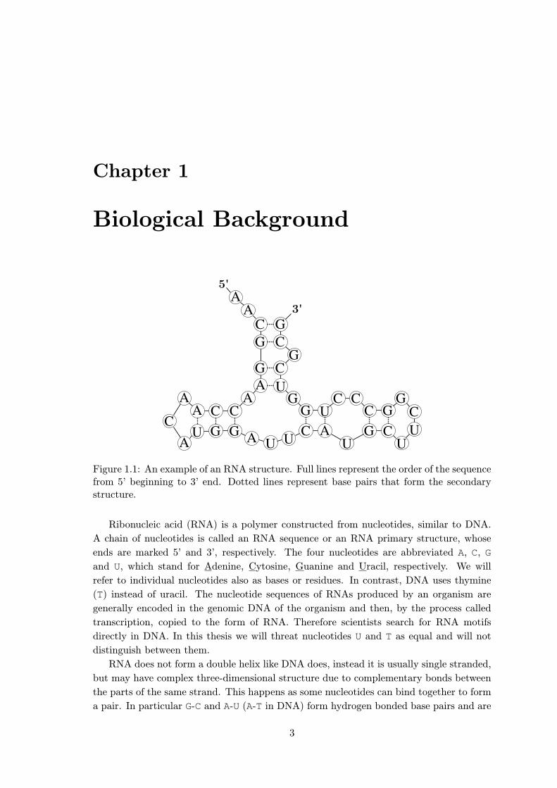
Figure 1.1: An example of an RNA structure. Full lines represent the order of the sequencefrom 5’ beginning to 3’ end. Dotted lines represent base pairs that form the secondarystructure.
Ribonucleic acid (RNA) is a polymer constructed from nucleotides, similar to DNA.A chain of nucleotides is called an RNA sequence or an RNA primary structure, whoseends are marked 5’ and 3’, respectively. The four nucleotides are abbreviated A, C, Gand U, which stand for Adenine, Cytosine, Guanine and Uracil, respectively. We willrefer to individual nucleotides also as bases or residues. In contrast, DNA uses thymine(T) instead of uracil. The nucleotide sequences of RNAs produced by an organism aregenerally encoded in the genomic DNA of the organism and then, by the process calledtranscription, copied to the form of RNA. Therefore scientists search for RNA motifsdirectly in DNA. In this thesis we will threat nucleotides U and T as equal and will notdistinguish between them.
RNA does not form a double helix like DNA does, instead it is usually single stranded,but may have complex three-dimensional structure due to complementary bonds betweenthe parts of the same strand. This happens as some nucleotides can bind together to forma pair. In particular G-C and A-U (A-T in DNA) form hydrogen bonded base pairs and are
3

Chapter 1. Biological Background 4
said to be complementary. These two canonical base pairs are also known as Watson-Crickpairs, named after James D. Watson and Francis Crick, who discovered the helical DNAstructure in 1953. In addition to canonical base pairs, non-canonical pairs also occur inRNA secondary structure. The most common non-canonical pair is G-U pair, which isalmost as thermodynamically stable as Watson-Crick pairs. The base-paired structure iscalled the secondary structure of the RNA, and the form which it adopts in 3D space iscalled the tertiary structure. An example of an RNA secondary structure can be seen inFigure 1.1. For many purposes, the secondary structure is a good approximation of thetertiary structure as it contains enough information on the spatial structure, while keepingthe complexity and time performance of related algorithms at reasonable level.
The first widely known RNA function was its role of a passive intermediary messengerin the process of translation of proteins from DNA. In this scenario, RNA encodes infor-mation about the composition of a protein. Therefore this type of RNA is called codingRNA.
However, subsequent research has shown that there exist many RNAs that do notencode any protein. These types of RNA are called non-coding RNAs (ncRNA). Non-coding RNAs adopt sophisticated three-dimensional structures. They are involved in generegulation, RNA processing, and other roles. For this type of RNA, the structure to whichit folds in space is often more important that the actual sequence.
New technologies allow us to obtain DNA sequences of various species. Given knownexamples of functional RNAs, we would like to locate RNAs with similar function (ho-mologs) in newly sequenced genomes. One option is to use searches based purely onsequence similarity. However, often we obtain higher sensitivity by allowing sequence tovary and searching for certain typical structural motifs [Webb et al., 2009]. RNA struc-tural motifs generally define relative positions of base pairs in a secondary structure. Ourgoal is then to search for regions in DNA that could form the secondary structure pre-scribed by the motif.
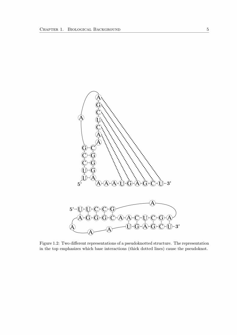
Base pairs in the RNA secondary structure typically form a number of short base-pairedstems (or also called as helices). Helices may overlap to form so-called pseudoknots. Thishappens when a helix starts before another one has already ended, this irregularity issimilar to an incorrectly parenthesized expression, e.g. “( [ ) ]”. An example of apseudoknotted structure is shown in Figure 1.2.
Pseudoknots make some computational problems harder, often being NP-complete[Durbin et al., 1998, Lyngsø, 2004]. Therefore for many purposes, as for example databasesearching for RNA homologs or RNA secondary structure prediction, it is usually ac-ceptable to sacrifice the information in pseudoknots in return for efficient algorithms[Durbin et al., 1998]. In this thesis we consider pseudoknots without any restrictions andthus allow arbitrarily pseudoknotted structures.
More formally, we can define a secondary structure of an RNA strand of length n
indexed 1 . . . n (starting at the 5’ end) as a set of pairing interactions (i, j) between i-thand j-th base of the strand, where every base may participate in at most one pair. Bythis definition, we can distinguish two fundamental elements of RNA secondary structure– single-stranded regions and helical (paired) regions.
Chapter 1. Biological Background 5
G CC GC GU GU A
A A A U G A G C5' 3'
AACUCGA
A
U
CG
GC
UA
UG
CG A A
UUA
CG
CG
GC
AU 3'
5'
A A A
A
Figure 1.2: Two different representations of a pseudoknotted structure. The representationin the top emphasizes which base interactions (thick dotted lines) cause the pseudoknot.

Chapter 1. Biological Background 6
1.1 Existing Search Tools
The problem of RNA structural motif search was first addressed in late 1980s. The firsttool enabling the structural search was RNAMot [Gautheret et al., 1990], which intro-duced a backtracking method. RNAbob [Eddy, 1996] is its more efficient reimplementa-tion based on a nondeterministic finite state automaton with node rewriting rules. After-wards, numerous stand-alone and web-service based tools were developed allowing usersto define RNA motifs according to their requirements and search for these motifs in se-quence databases. These tools differ in the way a user defines a structure that is to besearched for, then in allowing and handling defects permitted in found matches (e.g. mis-matches, mispairing, insertions), and post-processing filters applied on found matches. Ex-amples include Palingol [Billoud et al., 1996], RNAMotif [Macke et al., 2001], PatSearch[Grillo et al., 2003], RNAMST [Chang et al., 2006], Locomotif [Reeder et al., 2007]; foran extensive overview of current search tools see [George and Tenenbaum, 2009]. Besidesgeneral-purpose motif search tools, tools optimized for search of specific structural RNAmolecules were devised as well, e.g. tRNAscan-SE [Lowe and Eddy, 1997].
In 2010 we implemented a new search tool RNArobo [Rampášek, 2010], which buildson the motif format developed for RNAMot and RNAbob, but in addition enables a user topermit insertions to the structure. Algorithms searching for motifs including pseudoknotsin general have exponential time complexity. In 2011 we proved the RNA secondarystructure motif search problem to be NP-complete [Rampášek, 2011]. This proof is thesubject of the next chapter.

Chapter 2
Computational Complexity
In this section we formally define the problem in a form suitable for the analysis of com-putational complexity. It is important to note here, that search tools usually solve a moregeneral problem. Our simpler definition captures the essence of the problem and sufficesto show its NP-hardness. First, we will define a structural motif – an abstraction of RNAstructural motif.
2.1 Structural Motif
Structural motif specifies both primary and secondary structure constraints. The primarystructure deals with sequence constraints, while the secondary structure describes the rela-tions of the nucleotide bases forming the primary structure. By the definition of secondarystructure as a set of base pairings, we can distinguish two fundamental elements of RNAstructure – single-stranded regions and helical (paired) regions. On this observation weare going to built the definition of a structural motif, as an abstraction of RNA structuralmotif. First we introduce necessary terminology.
Sequence A = a1 . . . an is a string over a finite alphabet Σ.Sequence constraint alphabet Σ+ will be used to express constraints on primary struc-
ture and we define it asΣ+ =
(P (Σ) r {∅}
)∪{{∗}}
where ‘∗’ is a wildcard which matches every character from Σ or may be omitted, so thatpatterns of variable length are possible. Note that Σ+ is not a set of characters, but a setof sets of characters.
Fitting function FIT describes which symbols satisfy a given sequence constraint:
FIT : Σ+ × Σ→ {0, 1}
∀s ∈ Σ+,∀a ∈ Σ
FIT (s, a) =
{1 iff a ∈ s ∨ s = {∗}0 otherwise
We will state later on, how a wildcard ‘∗’ may be left out.
7

Chapter 2. Computational Complexity 8
Single-stranded element S = s1 . . . sn is a string over the alphabet Σ+.Helical element (H,H ′) represents a paired region, thus consists of two parts H and
H ′. Both H = s1 . . . sm and H ′ = s′1 . . . s′m are strings of the same length m ∈ N over the
alphabet Σ+.In a valid occurrence of a helical element (H,H ′) in a sequence, the matched occur-
rences of H and H ′ must be complementary, i.e. to form pairs character by character.To respect how a motif folds, we have to take the matched occurrence of H ′ in reverseorder, thus the first matched character of H must pair with (be complementary to) the lastmatched character of H ′, and so forth. The relation “to be complementary” is expressedby a complementarity function COMP .
Complementarity function COMP is the same for all helical elements, however maydiffer for different instances of the problem. COMP (a, b) = 1 if a, b ∈ Σ are considered tobe complementary in the problem instance. Otherwise, COMP (a, b) = 0.
Structural motif M can now be defined as an ordered sequence of single-stranded andhelical elements. The position of an element in the ordered sequence corresponds to itsposition in the motif. Between the two strands of a helical element, there can be arbitrarynumber of single-stranded elements as well as parts or whole other helical elements. Thisallows arbitrary pseudoknotted structures. For example M = (H1, S1, H2, S3, H
′1, S4, H
′2)
would correspond1 to the motif represented in the Figure 1.2, starting from 5’ beginningand ending at 3’. Another example of RNA motif is shown in the Figure 2.1.
If we are speaking about sequence constraints of a motif M , we refer to the concate-nation of sequence constraints of all the elements which form the motif M .
2.2 Structural Motif Search Problem
We say that a structural motif M (in context of a complementarity function COMP )occurs in a sequence A, if and only if there exists an partial increasing function ϕ of thesequence constraint indices of motif M = m1 . . .md to the indices in sequence A = a1 . . . ae,that satisfies:
(i) the image of function ϕ is one continuous subinterval of indices in A
(ii) only wildcards ‘*’ may be omitted, i.e.
∀i : ϕ(i) =⊥ ⇒ mi = {∗}
(iii) every sequence constraint from M fits the character to which it is projected, i.e.
∀mi ∈M : ϕ(i) 6=⊥ ⇒ FIT (mi,mϕ(i)) = 1
(iv) for every helical element (H,H ′) from M :
(a) let Aϕ(H) = p1 . . . pl be the string of characters from A to which H is projectedin ϕ
1further specification of the elements is required

Chapter 2. Computational Complexity 9
3'
H1 {A, C, G, U} S1 {C, U}
H2 {A, C, G, U} S2 {*}
S4 {A, C} S3 {*}
H2 {A, C, G, U} H3 {C, G}
S5 {*} H1 {A, C, G, U}
S7 {*} S6 {G}
S8 {G, U} H3 {C, G}
''
'
the matched occurrence
the motif
AU
CG G
C U
AAG
UC5'
another representation of the occurrence
the sequence
AACACUAGGUGACUCU
Figure 2.1: An example of RNA motif and of its occurrence in a sequence. For simplicity,the elements are only one character long. The thick arrows represent a matching thatdefines the motif occurrence.

Chapter 2. Computational Complexity 10
(b) denote Aϕ(H′) = q1 . . . qk similarly
(c) Aϕ(H) and Aϕ(H′) must be of the same length, i.e. l = k
(d) Aϕ(H) and Aϕ(H′) must be complementary character by character in terms ofcomplementarity given by the function COMP , i.e.
COMP (pi, qk−i+1) = 1 for i = 1, 2, . . . , k
Structural Motif Search Problem (in abbreviation SMS ) is then a decision problemdefined as follows:
SMS : For given alphabet Σ, complementarity function COMP , structuralmotif M and sequence A decide, whether M occurs in A, i.e. whether thereexists a correct projection ϕ of M to A.
2.3 RNA Motif Search Problem
The RNA motif search problem is a special case of SMS problem over RNA alphabetΣRNA = {A,C,G,U}, with complementarity function COMPRNA allowing only the canon-ical base pairs (C-G and A-U). We name this problem RNA-SMS.
2.4 NP-completeness of RNA-SMS
Similarly to the previous section, we will first discuss the SMS problem, as it is moregeneral and allows us to perform the proof more illustratively. Afterwords we show howto modify the proof to prove NP-completeness of the RNA-SMS problem.
Our proof of NP-completeness of SMS is inspired by [Lathrop, 1994] where the authorproves Protein Threading Problem to be NP-complete.
2.4.1 SMS is NP-complete
It is easy to see that SMS is in NP. For an SMS instance Σ, A,M,COMP , we can non-deterministically guess a correct occurrence of the structural motif M in the sequence A,i.e. a projection ϕ of M to A, and then check its correctness in polynomial time.
We will prove NP-hardness by a reduction of ONE-IN-THREE 3SAT to SMS. ONE-IN-THREE 3SAT is known to be NP-complete [Schaefer, 1978]. It is a variant of the 3SATproblem with a restriction that every clause must be satisfied by exactly one literal. Ourgoal is to construct an encoding from ONE-IN-THREE 3SAT to SMS, i.e. to constructan equivalent instance of SMS for every instance of ONE-IN-THREE 3SAT. A solutionto the equivalent SMS instance, i.e. a mapping of a motif M to a sequence A, encodes asolution to the original ONE-IN-THREE 3SAT instance, i.e. a boolean assignment to thevariables such that the formula is one-in-three satisfied.
Let us consider a ONE-IN-THREE 3SAT instance: a formula I in conjunctive nor-mal form, where each clause is composed of exactly three literals. We will construct anequivalent instance of SMS: Σ, A,M,COMP , as follows.
Chapter 2. Computational Complexity 11
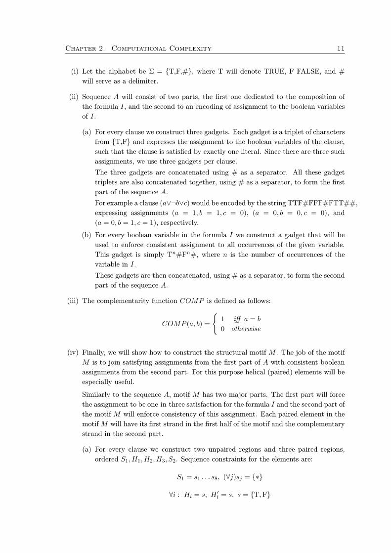
(i) Let the alphabet be Σ = {T,F,#}, where T will denote TRUE, F FALSE, and #will serve as a delimiter.
(ii) Sequence A will consist of two parts, the first one dedicated to the composition ofthe formula I, and the second to an encoding of assignment to the boolean variablesof I.
(a) For every clause we construct three gadgets. Each gadget is a triplet of charactersfrom {T,F} and expresses the assignment to the boolean variables of the clause,such that the clause is satisfied by exactly one literal. Since there are three suchassignments, we use three gadgets per clause.
The three gadgets are concatenated using # as a separator. All these gadgettriplets are also concatenated together, using # as a separator, to form the firstpart of the sequence A.
For example a clause (a∨¬b∨c) would be encoded by the string TTF#FFF#FTT##,expressing assignments (a = 1, b = 1, c = 0), (a = 0, b = 0, c = 0), and(a = 0, b = 1, c = 1), respectively.
(b) For every boolean variable in the formula I we construct a gadget that will beused to enforce consistent assignment to all occurrences of the given variable.This gadget is simply Tn#Fn#, where n is the number of occurrences of thevariable in I.
These gadgets are then concatenated, using # as a separator, to form the secondpart of the sequence A.
(iii) The complementarity function COMP is defined as follows:
COMP (a, b) =
{1 iff a = b
0 otherwise
(iv) Finally, we will show how to construct the structural motif M . The job of the motifM is to join satisfying assignments from the first part of A with consistent booleanassignments from the second part. For this purpose helical (paired) elements will beespecially useful.
Similarly to the sequence A, motif M has two major parts. The first part will forcethe assignment to be one-in-three satisfaction for the formula I and the second part ofthe motif M will enforce consistency of this assignment. Each paired element in themotif M will have its first strand in the first half of the motif and the complementarystrand in the second part.
(a) For every clause we construct two unpaired regions and three paired regions,ordered S1, H1, H2, H3, S2. Sequence constraints for the elements are:
S1 = s1 . . . s8, (∀j)sj = {∗}
∀i : Hi = s, H ′i = s, s = {T,F}

Chapter 2. Computational Complexity 12
A= FFF#TTF#TFT##FFT#TTT#TFF##...
M H11H12H13 H21H22H23
...T#F##TT#FF##TT#FF##T#F##
S11 S12 S21 S22
Figure 2.2: An example of the reduction. The figure shows a formula I, correspondingsequence A, and motif M . For better illustration the motif M is pictured also in aschematic way, to demonstrate how an occurrence of the motif encodes an assignment toboolean variables of I. The illustrated assignment is shown in the box in top part of thefigure.

Chapter 2. Computational Complexity 13
S2 = s1 . . . s8s9s10,
(1 ≤ j ≤ 8) sj = {∗}, s9 = {#}, s10 = {#}
The triplet H1, H2, H3 is intended to match in sequence A one of the threepossible assignments to the three variables forming the clause.
The two single stranded elements S1 and S2 are of variable length and allowthe triplet H1, H2, H3 to have enough freedom to be fitted to any of the threepossible assignments encoded in A. In addition, the element S2 ensures that thetriplet cannot be moved any farther, as it requires ## in the end.
(b) When constructing the first part of the motif, for every clause we left behindthe complementary parts of helix elements H ′1, H
′2, H
′3. We group all these H ′i
by the variable that is used in the i-th literal of the corresponding clause. For avariable x with k occurrences in formula I, we create a submotif starting with asingle stranded element Sx1, continuing with all H ′i elements corresponding to thevariable x and ending with a single stranded element Sx2. Sequence constraintsfor Sx1 and Sx2 are:
Sx1 = s1 . . . sk+1, (∀j)sj = {∗}
Sx2 = s1 . . . sk+1sk+2sk+3,
(1 ≤ j ≤ k + 1) sj = {∗},sk+2 = {#}, sk+3 = {#}
Note that Sx2 requires ## in the end. By this construction we enforce that theentire group of H ′i matches the block of Ts or the block of Fs in the sequence A.This denotes the assignment of TRUE and FALSE, respectively, to the variablex.
Recall, that in a valid occurrence of a paired element (Hj , H′j) must both Hj and
H ′j match the same character in A. Since the first parts of paired elements canonly match a one-in-three satisfiable assignment of a clause and the second partscorresponding to a variable x must all match the same boolean value, then a correctoccurrence of M indeed encodes a one-in-three satisfaction of the formula I.
An example construction is shown in Figure 2.2.In the instance of SMS, that we have just constructed, M occurs in A if and only if
the original formula is in ONE-IN-THREE 3SAT.The reduction is polynomial, since the construction of sequence A is linear2 in the
size of formula I, as well as the construction of motif M . Thus, if we could solve SMSin polynomial time, then we could solve also ONE-IN-THREE 3SAT in polynomial time.Since ONE-IN-THREE 3SAT is NP-complete, SMS is NP-complete, too.
2.4.2 RNA-SMS is NP-complete
The proof of RNA-SMS NP-completeness is analogous. Denote the corresponding sequenceA′ and motif M ′.
2For grouping all H ′i by the corresponding variable we can use counting sort, that has linear complexity.
Chapter 2. Computational Complexity 14
= GGGUCCGUCGCUUGGCUCCCUCGGUU...
H11H12H13 H21H22H23
...GUCUUGGUCCUUGGUCCUUGUCUU
S11 S12 S21 S22
A= FFF#TTF#TFT##FFT#TTT#TFF##...
M H11H12H13 H21H22H23
...T#F##TT#FF##TT#FF##T#F##
S11 S12 S21 S22
Figure 2.3: An example of the RNA-SMS reduction. Figure (a) shows sequence A anda sketch of motif M , both constructed in the original way from the SMS proof. Part(b) shows sequence A′ and a sketch of motif M ′ which form an instance of RNA-SMSequivalent to formula I.

Chapter 2. Computational Complexity 15
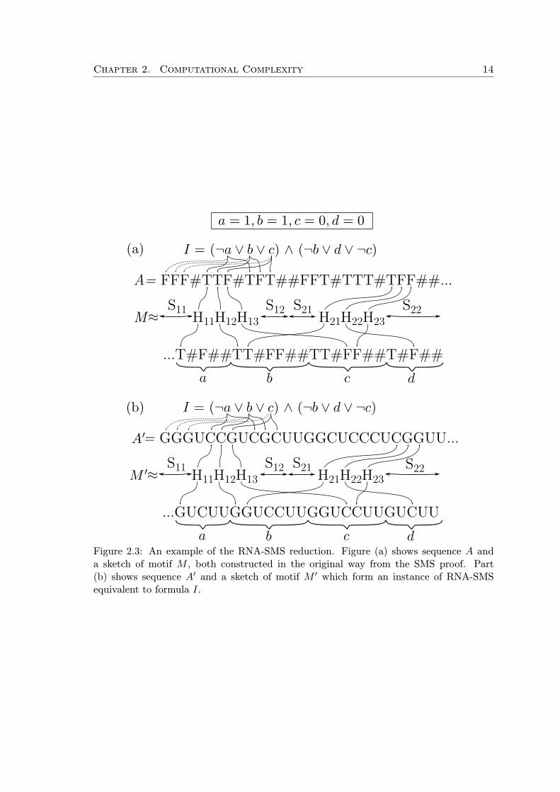
The construction of A′ and M ′ is the same as for SMS, with the following adjustments.
(i) In construction of motif M ′, we change {T,F} to {C,G} and {#} to {U} everywhereit is applicable.
(ii) In the construction of sequence A′ we substitute character # for character U. Whenencoding a possible one-in-three satisfiable assignment to variables of a clause, weencode TRUE as C and FALSE as G. In the second part of A′, where gadgets forassignment consistency enforcement are located, we switch the symbols, encodingTRUE as G and FALSE as C. This switch is necessary as the function COMP inthe SMS proof allows only pairs composed of the same two characters, howeverCOMPRNA allows only C-G, G-C, A-U, and U-A pairs. Since every paired elementfrom M ′ has the first strand in the first part of A′ and the second strand in thesecond part of A′, this construction of A′ is correct.
Figure 2.3 illustrates these changes and compares it to the original encoding used in theSMS proof.
Notice that the reduction remains polynomial. Therefore, we prove that RNA struc-tural motif search problem is NP-complete.
2.5 Discussion
Note that the proof described above could be also done by reduction from standard 3SAT.The main idea of encoding would remain the same. However, for every clause in theformula, we would construct seven, instead of three, gadgets encoding the satisfactoryassignments to the variables of the clause. This is because in 3SAT a clause has thecondition that the three literals must not be all FALSE at the same time. The number ofall satisfactory assignments is then at most 23 − 1 = 7.
Further, we identified two critical motif properties that govern the computational com-plexity of RNA structural motif search: (i) pseudoknots, and (ii) structural elements ofvariable length. Leaving out one of these properties would lead to an efficient searchalgorithm.
If we left out pseudoknots, we could use techniques of dynamic programming to proceedfrom short parts of the motif to the longer. This approach is similar to the RNA secondarystructure prediction algorithm discussed in [Durbin et al., 1998] and leads to polynomialtime complexity.
On the other hand, allowing only structural elements of fixed length, we could checkeach position in a sequence A for an occurrence of the motif M in linear time by asimple check of all primary and secondary constraints of M . Recall that the number ofthe constraints is linear in length of M . This approach would lead to quadratic timecomplexity in the length of A.

Chapter 3
RNArobo Algorithm
In the following, we recapitulate the search algorithm implemented in a software toolRNArobo. This algorithm was first introduced in [Rampášek, 2010] following the work of[Gautheret et al., 1990]. Our implementation was originally named RNAMot2, which welater changed to RNArobo. RNArobo can be used as a part of computational pipeline fordiscovery of RNA motifs [Jimenez et al., 2012]. In this thesis, we use the name RNArobofor the algorithm as well as for its implementation as a tool. It should be clear from thecontext which meaning are we referring to.
3.1 Algorithm Outline
An RNA motif is composed of several structural elements. We divide the algorithm intotwo parts:
(i) searching for occurrences of individual elements by a dynamic programming
(ii) assembling motif occurrences from the element occurrences by a backtracking search,which was first published as “Simple Scan” [Gautheret et al., 1990]
The approach is rather straightforward. Assume we search for a motif composed ofelements e1, e2, . . . , en. First, we select element e1 and search for its occurrences in thesequence. Once we have found one, we continue to search in its close neighborhood forelement e2. If there are multiple e2 occurrences, we fix the first one, and continue with theelement e3, and so further. This way we try to find a complete occurrence of the motif.In case element ei could not have been found in the corresponding neighborhood (or wehave already tried all its occurrences), we backtrack, and try the next occurrence of ei−1.The neighborhood to be searched for an individual element is determined in a way thatensures consistency of the overall motif match. An illustration of the search procedureis depicted in Figure 3.1. Note, that quality of the search does not depend on a chosenordering of elements in the search (we could use any permutation), however it affects therunning time in practice.
16

Chapter 3. RNArobo Algorithm 17
NNNN***** CNNN*****GG
AAGAAACTG NNN*****
****
********G
h1
s1
h2
s2
s3h1' h2' *****NNNG*****NNNN
search order: s1 s3 h2 h1 s2
s1 h2 s2 h2' s3 h1'h1
s1 h2 h2' s3 h1'h1
s1 h2 s3
s1 s3
s1
s1 h2 h2' s3
s1 s3
Figure 3.1: An illustration of RNArobo search procedure for a motif of ATP aptamer.The search follows the order of elements s1, s3, h2, h1, s2.

Chapter 3. RNArobo Algorithm 18
� �h1 s1 r2 s2 r2’ s3 h3 s4 h3’ s5 h4 s6 h4’ h1’ s7
h1 0:2 NNNNNNN:NNNNNNNr2 0:1 *NNN:NNN* TGCAh3 0:1:1 NNNNN:NNNNN:Ah4 0:1:1 NNNNN:NNNNN:Rs1 0 TNs2 0 NNNN[10]s3 0 Ns4 1 NNSGYN*s5 0 NN[20]s6 0 TTC****s7 0:1 NCCA:A
R s7 h4 s6 h3 h1 r2 s1 s4 s3 s2 s5� �Listing 3.1: Modified descriptor of a tRNA cloverleaf to demonstrate the descriptor syntax.The first line of the descriptor is the motif map, then specifications of individual elementsfollow, and in the last line is a command defining the order of elements in the RNArobosearch.
3.2 Descriptor Format
Let us now proceed with the specification of the input format of an RNA motif, called a de-scriptor. RNArobo uses a slightly augmented descriptor format of RNAbob [Eddy, 1996].Thanks to this, RNArobo is compatible with RNAbob descriptors. An example of RNArobodescriptor is shown in Listing 3.1.
A descriptor consists of two main parts:
(i) a motif map – a list of structural elements, which establishes the motif composition
(ii) a detailed specification for each of the structural elements
In the motif map, we enumerate the elements in such ordering, as they occur in themotif from the beginning to the end. Identifiers of single strand elements are denoted bythe prefix s, while paired elements use the prefix h or r (the difference between thesetwo will be clarified shortly). The rest of the identifier may be arbitrary, yet unique,alphanumeric word. Furthermore, since paired elements are composed of two strands,identifiers for both primary and complementary strand must be placed in the motif map.Identifier for the complementary strand is denoted by an apostrophe at the end, i.e. thecomplementary strand for h1 is h1’. The primary strand must precede its correspondingcomplementary strand, but we place no other restrictions on the relative order of individualelements in the map. This way, arbitrary pseudoknotted structures are possible.
The second part of the descriptor provides exact specification of all the elements, oneper line. For a single strand element sName of length m, the format is as follows:
sName M:I S1S2 . . . Sm:SI
The sequence constraints for this element are specified by S1S2 . . . Sm, where Si is anupper-case latter specifying a set of admissible residues for position i according to the

Chapter 3. RNArobo Algorithm 19
IUPAC notation1. Alternatively, Si can be a wildcard denoted as *, which allows foreither zero or one copy of letter N at this position (N matches all residues). This way,elements of variable length can be specified. To specify a long variable sequence, the usersimply writes a number n in square brackets instead of n asterisks (see element s5 inListing 3.1). Further, in the specification is defined the number of allowed mismatchesM and insertions I in the element. Letter SI specifies according to the IUPAC notationwhich nucleotides are allowed as an single-nucleotide insertion (e.g. there is one insertionof A allowed in element s7 in 3.1). The specification of I and SI is optional, and canbe omitted. In that case, none insertion is allowed. If insertions are allowed, we putrestrictions on their position. Insertions are forbidden to occur before the first or after thelast symbol of the element. Furthermore, adjacent insertions are forbidden as well.
Specification of a paired element is analogous:
hName M:R:I S1S2 . . . Sm:S′mS′m−1 . . . S
′1:SI
Compared to single strand specification, we add sequence constraints S′m . . . S′1 for the
complementary strand, and the number of mispairs R. Similarly to single strand elements,the insertions are not allowed at the beginning and after the end of the element. Further,insertions must not be adjacent nor opposite in context of the paired element. This is aso-called helical element, as it has the prefix h. We mentioned earlier that another kindof paired element is also possible. It is a so-called relational element denoted by a prefixr. Relational elements are generalized helical elements, where we can specify an arbitrarycomplementarity function by a transformation matrix. A transformation matrix specifiesthe rule, according to which bases complementary to A-C-G-T are determined. For example,if we want to allow for canonical, and G-T pairings, the corresponding transformationmatrix is TGYR (Y stands for T or C, and R stands for T or A). This TGYR transformationmatrix is implicit for helical elements. The following relational element specification isthen equivalent to the previous helical element:
rName M:R:I S1S2 . . . Sm:S′mS′m−1 . . . S
′1:SI TGYR
Optionally, element reordering command can be placed in the last line of the de-scriptor. In the backtracking search, elements will then be used in this particular ordering.This command has no effect on the quality of RNArobo search, however the element order-ing can significantly influence the performance. We devote Chapter 4 to the problematicof finding an ordering that leads to short execution time.
3.3 Dynamic Programming for Single Strand Elements
In this section we describe a dynamic programming algorithm which finds all occurrencesof a single strand pattern P in a text T with at most M mismatches and I insertions ofa one-letter-long pattern PI .
We use four dimensions of a five-dimensional table S to keep track of position in
1see Appendix A on the page 53

Chapter 3. RNArobo Algorithm 20
T , position in P , the number of occurred mismatches, and the number of insertions,respectively. The fifth dimension is binary, and is intended to serve as a flag, whether theprevious aligned symbol of T is an insertion, as one insertion cannot follow another.
Formally, we define a function S as follows:
St,p,m,i,b ∈ {0, 1} ;
t ∈ {0 . . . |T |} , p ∈ {0 . . . |P |} ,m ∈ {0 . . .M} , i ∈ {0 . . . I} , b ∈ {0, 1}
St,p,m,i,b =
1 iff P [1 . . . p] can be aligned with a suffix of T [1 . . . t]
with m mismatches, and i insertions;if b = 1 then T [t] is an insertion
0 otherwise
Recurrence
In [Rampášek, 2010] we proposed the following recurrence to compute the function S.
Initial conditions: ∀t ∈ {0 . . . |T |} St,0,0,0,1 := 1
The recurrence:
St,p,m,i,0 =∨
∨b
St−1,p−1,m−x,i,b x := (int)(T [t] does not fit P [p])
St,p−1,m,i,0 iff P [p] =‘∗’ (skip a wild card)
St,p,m,i,1 =∨
St−1,p,m,i−1,0 iff T [t] fits PI (an insertion)
St,p−1,m,i,1 iff P [p] =‘∗’ (skip a wildcard)
Solutions:
A match of the pattern P is found in the text T ending at position t ≤ |T |with m ≤M mismatches and i ≤ I insertions if St,|P |,m,i,0 = 1. To obtain thismatch we have to trace back.
3.4 Dynamic Programming for Paired Elements
The problem in this case is to find all occurrences of a paired pattern P : P ′ where P , P ′
are patterns of individual strands (i.e. |P | = |P ′|) in a text T , such that in an admissiblematch the individual strands are complementary.
Furthermore, we allow for imperfect matches with up to M mismatches, R mispairings,and with at most I insertions of a one-letter-long pattern PI together in both strands.
To address this pattern matching problem, we proposed in [Rampášek, 2010] a functionH, and a recurrence formula for its computation.

Chapter 3. RNArobo Algorithm 21
The function H for paired (helical) elements is the following:
Ht1,t2,p,m,r,i,b ∈ {0, 1} ;
t1, t2 ∈ {0 . . . |T |} , p ∈ {0 . . . |P |} ,m ∈ {0 . . .M} , r ∈ {0 . . . R} , i ∈ {0 . . . I} , b ∈ {0, 1}
Ht1,t2,p,m,r,i,b =
1 iff P [1 . . . p] can be aligned with a suffix T ′ of T [1 . . . t1] withm mismatches, P ′[1 . . . p] can be aligned with a prefix T ′′
of T [t2 . . . |T |] with no mismatch, T ′ and T ′′ contain togetheri insertions, and between T ′ and T ′′ are r mispairings;if b = 1 then exactly one of T [t1], T [t2] is an insertion
else none of the T [t1] and T [t2] is an insertion
0 otherwise
Recurrence
Initial conditions: ∀t1, t2 ∈ {0 . . . |T |} Ht1,t2,0,0,0,0,1 := 1
The recurrence:x := (int)(T [t1] does not fit P [p])
y := (int)(T [t2] is not complement of T [t1])
Ht1,t2,p,m,r,i,0 =∨
∨b
Ht1−1,t2+1,p−1,m−x,r−y,i,b iff T [t2] fits P ′[p]
Ht1,t2,p−1,m,r,i,0 iff P [p] =‘∗’1 (skip a wildcard)
Ht1,t2,p,m,r,i,1 =∨
Ht1−1,t2,p,m,r,i−1,0 iff T [t1] fits PI (an insertion)
Ht1,t2+1,p,m,r,i−1,0 iff T [t2] fits PI (an insertion)
Ht1,t2,p−1,m,r,i,1 iff P [p] =‘∗’1 (skip a wildcard)
Solutions:
A match of the pattern P : P ′ is found in the text T , P ending at positiont1 ≤ |T |, P ′ beginning at position t2 ≤ |T | with m ≤M mismatches, r ≤ Rmispairs, and i ≤ I insertions if Ht1,t2,|P |,m,r,i,0 = 1. To obtain this match wehave to trace back.
1In a correct paired pattern holds: ∀k (P [k] =‘∗’ ⇔ P ′[k] =‘∗’)

Chapter 3. RNArobo Algorithm 22
3.5 Implementation Note
RNArobo is implemented as a C++ console application, and is available for download athttp://compbio.fmph.uniba.sk/rnarobo/.
We have undertaken several optimizations of the code. Worth mentioning is optimiza-tion of the tables used in dynamic programming. These tables are typically sparse, withrelatively many zero elements. In the previous versions, we represented elements of thetable as arrays of coordinates and stored them in a red-black tree (C++ STL Set). Now,we encode the element coordinates into one 64bit integer. We also tried to replace thered-black trees by hash sets, but this change did not bring intended speed-up in practice(this can change with a better implementation).
Nevertheless, the most important enhancement is a new method for element orderingin the backtracking search, more on this method follows in the next chapter.
For more details on RNArobo algorithm and implementation we refer the reader to[Rampášek, 2010].

Chapter 4
Element Ordering in RNArobo
Ordering of motif elements in the RNArobo backtracking search has a significant impacton the execution time. To design a good element ordering of a complex motif is not asimple task, as many aspects are involved. Therefore we propose a data-driven methodfor finding a close-to-optimal element ordering, which leads to execution time as short aspossible.
4.1 Method Outline
Our approach consists of two main parts:
(i) heuristic proposal of possible orderings
(ii) data-driven evaluation of the proposed orderings
First, we generate all possible starting k-tuples of elements (where k is a parame-ter). These k-tuples are scored by a heuristic scoring function which takes into accountinformation content of the elements and their relative position within the motif.
All the k-tuples with scores above some threshold are augmented to complete searchorderings by the information content heuristic. Then we take random samples from this setand run the motif search with the sampled ordering in a sequence window of a fixed size.For each such application of an ordering, we measure the number of memory operations ofthe underlying dynamic programming as an approximation of the execution time. Basedon the gathered data, we continually eliminate orderings with bad performance. In thisway we progress in the search task window by window, but at the same time we observewhich orderings lead to the shortest execution times and adapt our strategy.
Additionally, after fixing the first k-tuple of the search ordering, we subsequently usethe same technique to find the best successive k-tuple (with respect to the already fixedordering prefix), and so on, until the whole search order is fixed.
4.2 Heuristic Scoring Function
The main goal of the heuristic evaluation of the proposed k-tuples is to select from all thepossible k-tuples a subset, which is small enough to be empirically evaluated. We want
23

Chapter 4. Element Ordering in RNArobo 24
this subset to contain at least some k-tuples that can be augmented to a complete elementordering with execution time not far from the optimum. Secondly, we would like not tohave many bad tuples in this chosen subset, because as we will see later, their evaluationcan increase running time excessively. Naturally, we want this heuristic evaluation to beconsiderably faster than the empirical.
The score of a k-tuple is a weighted sum of heuristic scores for individual elements ofthe k-tuple. The weight of an element in this sum decreases exponentially with its distancefrom the beginning. This is because an element placed sooner in the search order tendsto be searched in longer portion of the sequence. Further, the element’s score is a linearcombination of two heuristic functions h1 and h2. Thus the score of a k-tuple (e1, . . . , ek)
can be expressed as
h(e1, . . . , ek) =k∑
i=1
2k−i(h1(e
i) + c · h2(e1, . . . , ei))
(4.1)
The first heuristic h1 is an approximation of the information content of an element,favoring elements that pose more specific constraints. The second heuristic h2 is order-sensitive and accounts for flexibility of the element’s search domain with respect to ele-ments preceding in the ordering. In practice, we use k = 3 and c = −0.3. After scoring allk-tuples we select those that achieve at least 85% of the maximal score achieved by someof the k-tuples. If there are too many good k-tuples, we limit them to the best 40, howeverthis is a parameter. In the next sections we discuss the heuristic functions in detail.
4.2.1 Information Content Heuristic
By this heuristic, we want to follow the fail-first1 heuristic generally used in backtrackingsearches [Russell and Norvig, 2010]. This heuristic says that we should search first for theelement, which is the least likely to occur. Thus we need to asses the restrictiveness of anelement with respect to genomic sequence in which we execute the search. As a measureof restrictiveness, we use information content of this element.
Information content is a measure of uncertainty reduction about an outcome once wehave received a new piece of information. In other words, it is the difference in the entropyof a random variable before and after some message has been received.
I = Hbefore −Hafter
Note, that I can have a negative value if after receiving a message the outcome of therandom variable is actually more random than we originally expected. Recall, that entropyof a random variable is defined as:
H(X) = −∑i
P [X = xi] lgP [X = xi]
Here we use logarithm with base 2, so the entropy corresponds to bits.In our case we assume the initial state to be a uniform distribution over DNA sequences
1also called minimum-remaining-values or most-constrained-variable-first heuristic
Chapter 4. Element Ordering in RNArobo 25
of a fixed length. When we are told that an occurrence of an element starts at the firstposition of a sequence, the distribution is changed from all genomic sequences to thosethat match the element. Therefore, the information content of an element is entropy ofthe background genomic sequence distribution minus the entropy of the distribution ofsequences that match the given element.
We compute an approximation of the information content, since exact entropy com-putation of an element with allowed insertions or with variable length is not trivial, and areasonable approximation is sufficient for our purpose. We approximate the informationcontent of an element as a sum of information contents of its individual positions and thenwe refine the result according to the number of insertions, mismatches, and mispairs (inpaired elements) allowed.
For an unpaired element, the background probability distribution of a residue is uni-form over the set {A,C,G,U}. Therefore the background entropy Hu
before(a) of an unpairedresidue a is:
Hubefore(a) = −
4∑i=1
1
4lg
1
4= lg 4 = 2 bits
Constraints, which an element puts at a particular residue ei, change the distribution inone of these 5 ways:
1. The element defines a residue ei without ambiguity, i.e. it allows only one residuefrom {A,C,G,U}:
Huafter1(ei) = − lg 1 = 0 bits
resulting in information content for such a position to be
Iu1 (ei) = Hubefore(ei)−Hu
after1(ei) = 2 bits
2. The residue ei must be from a subset of size 2 of {A,C,G,U}, in the IUPAC notation2
this is expressed by one character from {M,R,W,S,Y,K}:
Huafter2(ei) = − lg
1
2= 1 bit
Iu2 (ei) = Hubefore(ei)−Hu
after2(ei) = 2− 1 = 1 bit
3. The residue ei can take one of three specified values from {A,C,G,U}, in the IUPACnotation this is expressed by a character from {B,D,H,V}:
Huafter3(ei) = − lg
1
3= 1.585 bits
Iu3 (ei) = Hubefore(ei)−Hu
after3(ei) = 2− 1.585 = 0.415 bits
4. There is no restriction on the residue ei (it can take any value), in the IUPAC
2see Appendix A

Chapter 4. Element Ordering in RNArobo 26
notation this is expressed by character N:
Huafter4(ei) = − lg
1
4= 2 bits
Iu4 (ei) = Hubefore(ei)−Hu
after4(ei) = 2− 2 = 0 bits
5. Finally, the constraint for ei can be a wildcard (it can take any value or to beomitted), expressed by character *. We assume all the possibilities to be equallylikely, therefore:
Huafter5(ei) = − lg
1
5= 2.322 bits
Iu5 (ei) = Hubefore(ei)−Hu
after5(ei) = 2− 2.322 = −0.322 bits
Here we have the situation, when the outcome is actually more random than we haveexpected.
Information content I ′unpaired(e) of an unpaired element e with no mismatch or insertionallowed is then
I ′unpaired(e) =
|e|∑i=1
5∑j=1
[ei is of type j] · Iuj (ei) (4.2)
We will show how to deal with mismatches and insertions later on.For a paired element, we assess its information content as a sum of information
contents of the individual pairs that form this element. The background probability dis-tribution of each pair is uniform, hence the entropy Hp
before(b) of a pair b is:
Hpbefore(b) = −
42∑i=1
1
42lg
1
42= − lg
1
42= 4 bits
Let us now show how to compute Hpafter(ei). The distribution of possible pairs in a paired
position ei is influenced by the sequence constraints of the element, as well as by theconstraint that the two residues must be complementary. As mentioned in Chapter 1, inaddition to canonical pairs G-C, and A-U, the couple G-U is also often considered to forma pair. Hence in RNArobo we allow a user to define an arbitrary pairing function. Sincethere are only 16 possible pairs, we can iterate through all of them and verify whether theparticular pair satisfies both the conditions. Let us denote the number of such correct pairsr. Additionally, if the pair is (*,*), then there is one more option – to skip this pair (thisleads to negative information content for such a pair). Calculation is then straightforward:
Hpafter(ei) = −
r∑i=1
1
rlg
1
r= lg r bits
resulting in information content of the residue pair ei to be
Ip(ei) = Hpbefore(ei)−H
pafter(ei) = 4− lg r bits
Information content I ′paired(e) of an paired element e with no mismatch, mispair, nor
Chapter 4. Element Ordering in RNArobo 27
insertion allowed is then
I ′paired(e) =
|e|∑i=1
Ip(ei) (4.3)
In what follows we show how we approximate the impact of mismatches, mi-spairs, and insertions on the information content of an element. Intuitively, thesedistortions cause more sequences to match an element, i.e. they bring in more uncertaintyabout the result. Since we do not model them in the background distribution, they willcause negative gain in information content of an element.
Mismatch: A mismatch in an element causes some residue sequence constraint to matcheverything, i.e. it changes to N. To simulate this, we could find a most constrainedposition in the element, and subtract its information content from the overall infor-mation content. However, we simply subtract 2 bits as a flat rate.
Mispair: A mispair cancels the mutual connection between two paired positions. Wecould find a pair, whose information content would suffer the most from this loss ofpairing. However, we simply take the worst case, i.e. one residue used to unambigu-ously determine the other. This means loss of 2 bits of information, as one residue ofsuch a former pair does not impose any restrictions on the other residue any more.
Insertion: Insertions are hard to model, as they can occur almost anywhere in the el-ement, and the restriction that no two insertions can be adjacent, nor opposite inpaired regions make it even more complicated, as the insertions are not indepen-dent. Therefore we decided to model entropy of an insertion directly as the amountof information needed to specify its occurrence, and to neglect their dependency.
The first insertion in an unpaired element e may occur at m − 1 places, where mis the length of e, and at 2 · (m − 1) places in a paired element (as it has twostrands of length m). The number of positions where a successive insertion mayoccur differs according to where the preceding insertions occurred. We neglect thisfact and consider the number of positions for an insertion to remain constant. Tospecify where an insertion has occurred, we therefore need lg (m− 1), and lg (2m− 2)
bits, respectively. In addition, we need to specify what nucleotide was inserted. Torepresent this information we need additional 2, lg 3, 1, or zero bits, depending onwhat nucleotides are allowed for insertion (recall cases in computation of Hu
afterj).
For example, if only A is allowed to be inserted, we need no additional bits to codethis information, as it is implicit.
Now, we can refine previous estimates (4.2), and (4.3), to account also for the men-tioned distortions. Let us consider an element e of length m with nmm mismatches, andnins insertions of x allowed. If e is an unpaired element, its estimated information contentis:
Iunpaired(e) = I ′unpaired(e)−2nmm−nins
(lg (m− 1)+
4∑j=1
[x is of type j] ·Huafterj (x)
)(4.4)

Chapter 4. Element Ordering in RNArobo 28
If e is a paired element with nmp mispairs, then we estimate its information content as:
Ipaired(e) = I ′paired(e)− 2nmm − 2nmp − nins
(lg (2m− 2) +
4∑j=1
[x is of type j] ·Huafterj (x)
)(4.5)
Finally, we define the information content heuristic function h1(e) as follows:
h1(e) =
{Iunpaired(e) if e is an unpaired elementIpaired(e) if e is a paired element
(4.6)
4.2.2 Domain Flexibility Heuristic
In RNArobo search, when some element is already fixed and the algorithm tries to find anoccurrence of the next element, the position where it should occur is often not determineduniquely. Rather, it has to occur within an interval, which we call the search domain ofthe element. This happens because motif elements may be of variable length. The size ofa search domain of an element varies with respect to which elements have been alreadyfixed. The longer the domain is, the more time-consuming is the search for the elementoccurrence. Furthermore, we are likely to find more occurrences, which we will have toexamine individually in backtracking. This heuristic function is meant to reflect thesefacts.
The input to this heuristic is a non-empty `-tuple, ` ≤ k. We assume the first ` − 1
elements to be already fixed by the time the element e` is searched. Of course, we do notknown positions of matches of these preceding elements. However, the information thatthey are already fixed is sufficient to approximate the domain size of the element e`.
For an unpaired element e` we find the nearest fixed element ei (i.e. ei is one ofe1, . . . , e`−1) on the left side of e`. Then we sum up the flexibilities of all elements betweenei and e` in the descriptor. Flexibility of an element is the difference in its maximum andminimum length. We denote this sum Fleft. The same way we sum on the right side toobtain Fright. If there is not a fixed element at some side, we define the corresponding
Fside = 0. Then we approximate the domain size De1,...,e`−1
unpaired (e`) as
De1,...,e`−1
unpaired (e`) = min{Fleft, Fright}+ flexibility of e` + 1 (4.7)
where we also account for flexibility of the element itself, and plus one for the positionpresent in the domain without any flexibility. Notice that this approximation of the domainsize is always positive.
For a paired element e` composed of two strands e`first, e`second we proceed similarly.
First, we calculate De1,...,e`−1
unpaired (e`first), and De1,...,e`−1
unpaired (e`second) as in (4.7). In this computationof the domain size of one strand, we consider the other strand to be fixed. Since foran occurrence of one strand the complementary strand can occur at any position in itscorresponding search domain, the search domain size for e` is the product of domain sizes

Chapter 4. Element Ordering in RNArobo 29
for individual strands. Thus, we define De`,...,e`−1
paired (e`) for a double strand element as
De1,...,e`−1
paired (e`) = De1,...,e`−1
unpaired (e`first) ·De1,...,e`−1
unpaired (e`second) (4.8)
Finally, we define the domain flexibility heuristic function h2(e1, . . . , e`) as follows:
h2(e1, . . . , e`) =
{De1,...,e`−1
unpaired (e`) if e` is an unpaired element
De1,...,e`−1
paired (e`) if e` is a paired element(4.9)
4.3 Candidate Sampling
Recall that the heuristic function defined above is used to select promising initial k-tuplesfor search orders. These k-tuples are then augmented to complete search orderings by theinformation content heuristic. Denote the resulting set of complete orderings as O.
From O we uniformly choose independent and identically distributed (i.i.d.) samples.Subsequently we run the motif search with the sampled ordering in a sequence window ofa fixed size. For each sample x ∈ O, we measure Tx, the number of memory operations(read and write) of the underlying dynamic programming, as an approximation of theexecution time, which is universal for all machines. Each sequence window is used onlyonce. The next window shares an overlap with the previous one, so that the search cannotmiss a motif occurrence. This way we progress in the search task window by window, andat the same time we evaluate candidate orderings from O. In practice, we set the windowsize to be
max{10 ·max length of an occurrence, 1000}
However, it is not always possible to divide the searched sequences into windows of thesame size, especially when the search database contains many short sequences. Thereforewe normalize the number of measured memory operations by the actual window size, andwe use as Tx the number of memory operations per one base of a window.
We approximate the distribution of the random variable Tx by a Normal distributionwith unknown mean and variance. Examples of empirical distribution of Tx can be seenin Figure 6.2 in Chapter 6.
Our goal is to pick, from the set of candidate orderings O, the ordering which leadsto the shortest execution time on average. Formally, we want to find x∗ ∈ O, such that∀y, E[Tx∗ ] ≤ E[Ty]. We use Welch’s t-test (described in more detail in Section 4.3.1) totest the null hypothesis E[Tx] ≥ E[Ty] against the alternative hypothesis E[Tx] < E[Ty].Each time we gather a new sample from Tx for some x ∈ O, we run tests of x againstthe rest of O. Thus, as soon as we observe statistically significant difference between twocandidates, we can immediately eliminate the one with significantly higher mean time ofexecution from set O. In the case when the mean of two candidates cannot be comparedwith enough significance, even after both were sampled many times (we use threshold of100 samples from each), we break the tie. We simply eliminate the one with the highersampled mean.
In this way we sample and test until all but one ultimate ordering are eliminated, andwe have the winning initial k-tuple. Recall, that this initial k-tuple was extended to a full

Chapter 4. Element Ordering in RNArobo 30
ordering by the information content heuristic. Now, we can drop this extension and starttraining the following k-tuple in the ordering with already fixed prefix. In this way weprolong the fixed prefix, until we have a completely fixed order.
4.3.1 Details of Welch’s t-test
In this section we briefly describe the Welch’s t-test [Welch, 1947] used in our candidateelimination.
In statistics, the so-called Behrens-Fisher problem is the problem of hypothesis testing,which concerns difference between the actual means of two normally distributed popula-tions with possibly unequal variances, based on independent sets of samples from thesedistributions. This problem is a generalization of the Student’s problem that assumes thevariance of the populations to be equal. We decided to choose a method that can addressthe Behrens-Fisher problem, because in candidate elimination we cannot assume equalityof variances of variables Tx.
A variety of methods has been proposed to address this problem. They differ inrobustness against Type I errors under violations of normality, difference in the sam-ple groups sizes, or difference in the variances. For more details we refer the reader to[Kim and Cohen, 1998, Ruxton, 2006]. We decided to use the Welch’s t-test as it has thebest combination of performance and ease of use [Ruxton, 2006].
Welch’s t-test is based on Student’s t-test, which assumes the variances of the twopopulations to be equal. Welch proposed several methods to correct the number of degreesof freedom in Student’s t-test in case of unequal variances. Probably the most commonlyused approximation is the Welch-Satterthwaite equation, [Satterthwaite, 1946]. Thereforethis method is also called Welch-Satterthwaite test, or Smith/Welch/Satterwaite (SWS)test, acknowledging also the work of Smith [Smith, 1936]. However the most commonlyused name is simply “unequal variance t-test”.
Welch’s t-test, similarly to Student’s t-test, is comprised of calculating a t statisticthat is then compared with the value in standard t tables according to the appropriatenumber of degrees of freedom ν. The statistic t is defined by the following formula:
t =µ1 − µ2√s21n1
+s22n2
(4.10)
where µi is the sample mean, s2i the sample variance, and ni the sample size of the ith
population.The approximate number of degrees of freedom ν is then obtained form the Welch-
Satterthwaite equation:
ν =(g1 + g2)
2
g21n1−1 +
g22n2−1
where gi =s2ini
(4.11)
With this ν computed, we look-up the appropriate critical value of t in a table oft-distribution and execute a one-tailed test. If the computed t is greater than the criticalvalue, we reject the null hypothesis in favour of the alternative hypothesis. In our algorithmwe test at significance level α = 0.025.

Chapter 5
Post-processing of RNAroboResults
The fact that a piece of sequence matches an RNA structural motif is not sufficient toexpect that this sequence really folds into the desired structure. This happens becauseour search task represents only a very simplified model of the physical forces involved inRNA folding. To at least partially address this problem, we have implemented a set ofsoftware tools, which enable a user to sort and filter the found motif occurrences accordingto estimated structural stability. In this chapter, we use the term false positive for a matchthat is not correct in the context of searching for real homologs. Tools described in thischapter were developed under the guidance of Prof. Andrej Lupták. These tools areintended to mimic bioinformatic analyses that biochemists would do manually to verifythe functionality of proposed matches.
5.1 RNA Structure Prediction
Syntactical match of an RNA structural motif in RNArobo search does not imply thatthis desired structure is the most stable (probable) structure for this found piece of RNAsequence (the match). A natural way to address this issue would be to calculate the moststable structure of this sequence and then compare it to the desired structure.
Here comes the problem. We have to solve the RNA structure prediction problem, alsoreferred to as RNA folding problem. This problem has been thoroughly studied for pastdecades, leading to many different algorithms.
These algorithms often differ in definition of the optimal secondary structure theyare looking for. Usually, they seek to the structure in which the RNA sequence has thelowest minimum free energy (MFE), which tends to be the most stable structure. Theoriginal methods for MFE structures computation typically use combinatorial optimiza-tion techniques (e.g. dynamic programming). The most recognized algorithms in thisgroup are Nussinov algorithm [Nussinov and Jacobson, 1980], Zuker-Sankoff algorithm[Zuker and Sankoff, 1984], and McCaskill algorithm [McCaskill, 1990].
However there is evidence that RNA sequences start folding right away during theprocess of their transcription from DNA. This may cause a sequence to fold into a local
31

Chapter 5. Post-processing of RNArobo Results 32
optima different from the globally optimal MFE structure. Folding kinetics approachesaccount for this phenomenon, such as KineFold [Xayaphoummine et al., 2005].
Comparative methods try to exploit known structures of RNA sequences similar tothe query sequence. This method is suitable for sequences belonging to a known RNAfamily. To model the consensus structures of a given family and then to infer a structurefor the query sequence, algorithms mainly use stochastic context-free grammars, and theirvariations (e.g. covariance models).
Despite a lot of effort, accuracy of the exiting general-purpose methods is rather lowfor more complex structures. However, the main pitfall of RNA structure prediction arepseudoknots, as they cannot be directly modeled by stochastic context-free grammars orby common energy models. In fact, the general pseudoknot prediction has been provenNP-hard [Lyngsø, 2004]. Lately, many methods have been proposed to tractably addressthe pseudoknot prediction problem in practice also for longer sequences [Ren et al., 2005,Bellaousov and Mathews, 2010, Sperschneider and Datta, 2010, Sato et al., 2011]. Unfor-tunately, none of the existing general-purpose tools can reliably predict complex struc-tures, like the double pseudoknotted structure of the HDV ribozyme, which is particularlycomplicated.
Therefore to filter out false positives from RNArobo search results, we cannot simplyuse an RNA structure prediction tool, as we proposed at the beginning of this section.Besides the problem with the accuracy of the structure prediction, this approach hasone more drawback. Comparing the predicted structure to the structure prescribed bya descriptor is not trivial, because the real homologous motif occurrences seldom shareexactly the same structure. Slight structural variations in some parts of the motif arepermissible, while some parts of the motif are crucial for the functionality, and are muchmore structurally and sequentially conserved. We try to model these phenomena in theRNArobo search by allowing for mismatches, mispairs, insertions, or wildcards, that causethe search to be more sensitive however less specific. It is therefore crucial to accountfor this variability or strictness of individual parts of the RNA motif primarily in post-processing phase. Naturally, expert knowledge on the searched RNA motif is necessaryfor more precise in silico evaluation of the candidates, proposed by RNArobo search.
5.2 Evaluation of Structural Stability per-partes
Our approach allows a user to select several submotifs of the searched motif. For eachsuch submotif we use external tools for RNA structure prediction and based on the resultwe assign it some score. The score of a motif occurrence is then a linear combination ofsubmotif scores.
These submotifs do not have to be continuous in the motif, nor they have to bemutually disjunct, i.e. a submotif can be an arbitrary list of structural elements presentin the motif. It is advisable to select submotifs, whose structure can be predicted withsufficient accuracy. For a particular motif occurrence, nucleotide sequences belonging tothe individual elements are parsed out, and for each submotif the corresponding sequenceis assambled together. We then compute a predicted structure (fold) and its minimumfree energy (MFE), using ViennaRNA package [Hofacker et al., 1994, Lorenz et al., 2011],

Chapter 5. Post-processing of RNArobo Results 33
and DotKnot [Sperschneider and Datta, 2010] in case of pseudoknotted submotifs. Scoreof each submotif is then computed by one of the following ways:
(i) stability of the predicted fold, the score is the absolute value of the predicted MFE
(ii) stability of the predicted fold in terms of the predicted MFE per one base
(iii) closure of the predicted fold, the score is the percentage of first n bases of the submotifthat pair with last n bases of the submotif
The score of the motif occurrence is then a linear combination of submotif scores. Theparameters of the linear function are defined by the user. Recall that the submotifs can bearbitrary, e.g. a user can define the same submotif twice and use different score functions.For example, this could lead to scoring the submotif according to its MFE as well asaccording to its fold closure at the same time.
We have implemented this method in a tool called FoldFilter. It allows an expert userto assess RNArobo search results, and filter out majority of false positive matches. Thebest occurrences are then good candidates for further in vitro testing.
To facilitate estimation of the submotif weights we introduce a tool called Weight-sTool, which allows the user to dynamically change these weights and see how the changesaffect the score distribution over all motif occurrences. It is then possible to export alloccurrences with score over a desired threshold.
5.3 Implementation Note
Both tools for post-processing of RNArobo results, FoldFilter and WeightsTool, are imple-mented as Perl scripts. They are available for download at the official RNArobo website:http://compbio.fmph.uniba.sk/rnarobo/.
Prerequisites:
• properly installed ViennaRNA package
• DotKnot (provided in the script package)
• Python interpreter to run DotKnot
• Perl interpreter to run FoldFilter and WeightsTool
Functionality of the tools was tested in various Linux and Mac OS environments.
Chapter 6
Experimental Results
In this chapter we present empirical results obtained by running RNArobo on real biologi-cal sequences with several realistic descriptors. First we test validity of several assumptionsmade in Chapter 4. We then compare the overall running time of RNArobo with severalexisting tools and study the progress of ordering elimination in our data-driven elementordering (DDEO) strategy.
6.1 Used RNA Motifs
In our experiments we used the following four RNA motifs, their descriptors are listed inAppendix B.
• Motif of an ATP aptamer : A rather simple motif with a conserved single-strandedelement, but also with some elements of variable length. An illustration of the motifis depicted in Figure 3.1.
• Motif of a Hepatitis Delta Virus ribozyme’s double pseudoknot: This is the mostcomplex motif in our set. It contains sequentially conserved elements as well asvariable elements, and helices with allowed mispairs. But above all, it is the doublepseudoknot that makes the motif complicated.
• Motif of a Hammerhead ribozyme: In the motif there are single-stranded elementsthat are sequentially conserved, but also two very variable elements. Helices are alsoof variable length, but a perfect canonical pairing is required.
• Generalized motif of a tRNA cloverleaf : This motif contains structural elementsof variable length and helices with allowed mispairs. These properties with lack ofsequential conservation slow down the search, and cause the motif to have manymatches.
34
Chapter 6. Experimental Results 35
6.2 Used Genomic Sequences
We have used real DNA sequences:
• Genome of a fruit fly (Drosophila melanogaster) [NCBI, 2012a]. This database is168,736,537 bases long.
• Human genome [NCBI, 2012b], that is 3,137,161,264 bases long.
6.3 Hardware and Software Environment
As a machine for our tests, we used a server with eight physical cores (2× quad-core IntelXeon E5520 @ 2.27GHz), and 16GB of RAM.
The operating system was Ubuntu Server 10.04.4 LTS. For compilation of C/C++source code we used GCC 4.4.3 compiler with optimization level 3 (-O3 flag).
6.4 Memory Operations vs. Real Time
As mentioned earlier in Section 4.3, we use the number of memory operations done duringdynamic programming as a measure of the real execution time in DDEO. By a memoryoperation we mean any access to the dynamic programming table, i.e. both read and writeoperations are counted equally. We have run several experiments to demonstrate that thismeasure correlates well with the real execution time.
We have chosen 9 different search orders of elements in the tRNA motif. Then witheach of these fixed orderings we have run RNArobo search in a fixed ∼2.2 million bases longsequence. We measured both execution time and memory operations. In Figure 6.1 weplotted the average number of memory operations per second for each of these experiments.The execution time varied from a few second to several minutes, however the ratio ofmemory operations per second stays rather steady. Note that the ratio slightly variesdue to the influence of all the other operations that are involved, as in these experimentswe measured the total execution time, including input parsing, overhead of backtrackingsearch, and so forth.
These results encourage us to use the number of memory operations as a good machine-independent measure of the execution time for the purpose of our data-driven elementordering method.
6.5 Normality of Tx
In our DDEO strategy (Section 4.3) we measure the number of memory operations as ameasure of the execution time and then we use such observations to eliminate search ordersby a statistical test. Here we test the normality of the variables involved in this test. Recall,the random variable Tx for an order of elements x, is the number of memory operationsexecuted during RNArobo search in a sequence of a fixed size and then normalized bythis window size. In other words, Tx is the average number of memory operations per oneresidue in a sequence window. For the purpose of candidate elimination in Section 4.3

Chapter 6. Experimental Results 36
●
● ●
● ●
●
●●
●
2 4 6 8
0e+
001e
+06
2e+
063e
+06
4e+
065e
+06
experiment
mem
OP
s / s
econ
d
1 2 3 4 5 6 7 8 9
Figure 6.1: The the number of dynamic programming memory operations per one secondof the overall execution time in our 9 experiments does not vary significantly.
we assume Tx to have Normal distribution. We want to show that this assumption hasrational foundation.
We measured ∼530 samples of Tx for four different element orders of the tRNA motif.Although the measured values do not pass statistic normality tests, in Figure 6.2 we cansee that the Normal distribution is a good approximation.

Chapter 6. Experimental Results 37
5 10 15 20 25
0.00
0.02
0.04
0.06
0.08
0.10
0.12
memOPs
Den
sity
5 10 15 20 25
0.00
0.05
0.10
0.15
memOPs
Den
sity
300 350 400 450 500 550
0.00
00.
005
0.01
00.
015
0.02
0
memOPs
Den
sity
350 400 450
0.00
00.
005
0.01
00.
015
0.02
00.
025
memOPs
Den
sity
Figure 6.2: Sampled distributions of Tx (the number of memory operations per residue)on different sequence windows using four different fixed orders of elements. In each plot,the blue curve is a kernel density estimation of the Tx samples using uniform (rectangular)kernel. In red is depicted the Normal distribution with parameters set to sample meanand sample variance.

Chapter 6. Experimental Results 38
6.6 Execution Time
In this section we compare the running time of RNArobo with data-driven element ordering(RNArobo 2.0) to the previous RNArobo version 1.94, and to established search toolsRNAbob 2.2 (1999) [Eddy, 1996], and RNAmotif 3.0.7 (2010) [Macke et al., 2001]. Note,that RNArobo 1.94 uses a fixed search ordering obtained by a simple heuristic, and isotherwise identical to RNArobo 2.0.
We have measured three runs of RNArobo 2.0 (with DDEO), and then run the searchagain with the best search order found in individual runs. This way we can assess thequality of found orderings as well as the overhead of the DDEO, which fluctuates asrandomization is involved.
In DDEO, we use the following parameter values:
• k = 3
• cutoff score for k-tuples is 85% of the maximum score
• limit for O is |O| ≤ 40 (if there is too many good candidates over cutoff threshold)
• window size is max{10 ·max length of a motif occurrence, 1000}
• significance level for Welch’s t-test is α = 0.025
After fixing the first triplet of the search order, we use the same technique to find the bestsuccessive triplet, and so further, until the whole search order is fixed.
Elimination of candidates by Welch’s t-test at significance level α = 0.025 appears tobe the best trade-off between stability and execution time. Testing with higher α tends tobe less stable. The search converges to a final ordering rather quickly, however mistakesleading to worse ordering are more likely to happen. On the other hand, lower α forcesthe search to execute more samples, including those with inferior performance.
There may not be one unique ordering that is significantly better than all the others,therefore we break ties between two orderings, after each has more than 100 samples, byeliminating the ordering with the higher sample mean.
We have conducted three sets of tests:
• on chromosome 3 of the Drosophila genome (27,905,053 bases; Figure 6.3)
• on the whole genome of a Drosophila (168,736,537 bases; Figure 6.4)
• on the whole human genome (3,137,161,264 bases; Figure 6.5)
In each test, we scanned both strands of the DNA, thus doubling the effective sequencelength. We tested RNArobo 1.94, a version with unsophisticated heuristic for elementordering, only in the first test set. As can be seen in Figure 6.3, this heuristic works wellfor a simple motif of ATP aptamer, but for more complex structures it fails to deliver areasonable ordering. Thus we left out RNArobo 1.94 from the genome-wide tests.
In Figure 6.3 we use a relatively short sequence, and for a complex motif, such asHammerhead ribozyme, RNArobo with DDEO needs a much longer time than RNAroborun with the best order already given at the start. This is due to bad candidate orders,

Chapter 6. Experimental Results 39
whose empirical evaluation is time-consuming. However notice, that DDEO overheadis roughly constant with respect to the length of the searched genomic sequence. Aswe increase the sequence length (Figures 6.4 and 6.5), we can see that this overhead isbecoming negligible. Therefore in case of search in large database, e.g. genome-widesearch, it is advisable to sacrifice longer DDEO overhead in return for better ordering,which eventually leads to shorter execution time.
We can see that RNArobo 2.0 even with DDEO overhead outperforms RNAbob andRNAmotif in case of complex motifs like HDV pseudoknot and tRNA. In this case RNArobobenefits from the ability to find a close-to-optimal search ordering, and also from its ro-bust underlying dynamic programming. For the other two motifs, RNArobo 2.0 is slightlyslower than RNAbob, and RNAmotif performs far the best. Notable is the rather steadyperformance of RNArobo throughout the whole test set. For example the difference inRNAmotif performance for ATP aptamer and for HDV pseudoknot is enormous, whilefor RNArobo the difference is fairly small. This shows, that the bottleneck of RNAroboperformance is now the dynamic programming used in search for individual element oc-currences. RNArobo 2.0 does not use any pre-filtering techniques, or specialized patternmatching algorithms in case there are no mismatches or mispairs allowed in an element,but always uses the general dynamic programming. Thus we believe there is still room forfurther optimization.
0
50
100
150
200
250
ATPaptamer HDVpseudoknot HHribozyme tRNA
Ex
ecu
tio
n T
ime
(sec
.)
1,523 367 342 50,946 9,064
RNArobo + DDEO run1
RNArobo w/ the found order1
RNArobo + DDEO run2
RNArobo w/ the found order2
RNArobo + DDEO run3
RNArobo w/ the found order3
RNArobo 1.94
RNAbob 2.2
RNAmotif 3.0.7
Figure 6.3: Execution time of RNArobo 2.0 (with DDEO) compared to its previous version1.94, RNAbob 2.2, and RNAmotif 3.0.7. The search was conducted on chromosome 3 of theDrosophila genome (55,810,106 bases scanned). Element ordering heuristic in RNArobo1.94 fails to find an effective order for more complex structures. New data-driven methodin RNArobo 2.0 works well, however the overhead is notable as the sequence is short.

Chapter 6. Experimental Results 40
0
200
400
600
800
1,000
ATPaptamer HDVpseudoknot HHribozyme tRNA
Ex
ecu
tio
n T
ime
(sec
.)2,153 1,879
RNArobo + DDEO run1
RNArobo w/ the found order1
RNArobo + DDEO run2
RNArobo w/ the found order2
RNArobo + DDEO run3
RNArobo w/ the found order3
RNAbob 2.2
RNAmotif 3.0.7
Figure 6.4: Search in the genome of Drosophila (337,473,074 bases scanned). We compareRNArobo 2.0 to RNArobo with fixed previously found order, RNAbob 2.2, and RNAmotif3.0.7.
0
5,000
10,000
15,000
20,000
ATPaptamer HDVpseudoknot HHribozyme tRNA
Exec
uti
on T
ime
(sec
.)
37,273
RNArobo + DDEO run1
RNArobo w/ the found order1
RNArobo + DDEO run2
RNArobo w/ the found order2
RNArobo + DDEO run3
RNArobo w/ the found order3
RNAbob 2.2
RNAmotif 3.0.7
Figure 6.5: Execution time for the whole human genome search (6,274,322,528 basesscanned). The overhead of data-driven element ordering method in RNArobo 2.0 is neg-ligible for long databases.

Chapter 6. Experimental Results 41
6.7 Details of DDEO Operation
We devote this section to the analysis of operation of our data-driven element ordering(DDEO) method proposed in Chapter 4 and implemented in RNArobo 2.0. During thesearch for four motifs in the human genome described in the previous section, we recordedstatistics for all sampled candidates. Based on this data we want to explore how does theDDEO method progress in practice. The overall execution time of these searches can beseen in Figure 6.5.
For each of the four motifs we present two types of figures. The first type (e.g. Figure6.6) depicts the value of Tx averaged over windows where a particular ordering was used,i.e. it is the average number of memory operations per one base of a sampled window. Weplotted this value from three runs of RNArobo 2.0 for each of the best k-tuples that wereselected to set O (and augmented to complete element orders) based on our heuristicscoring function. Notice, that the heuristic proposal of the k-tuples is deterministic,therefore in each run the k-tuples are the same, however the sampled values from theirdistribution vary.
In the second type of figures we depict the number of samples done for each of theproposed k-tuples before it was eliminated or chosen as the very best k-tuple. We refer tothis number also as the coverage of a given k-tuple. In general, we can see the trend thatthe k-tuples with inferior performance have low coverage, as they are quickly eliminatedif there is a large enough proportion of candidates with a good performance (as it is thenmore likely that we sample a good candidate that will eliminate these inferior ones). Onthe other hand, the best performing k-tuples with similar values have higher coverage, asmore samples are required to eliminate one of them. Recall that we break tie between twok-tuples once we have obtained at least 100 samples of each.
In Figures 6.6 and 6.7 we can see artefacts of the DDEO method procedure in searchfor the best element ordering of the ATP aptamer motif. The performance of heuristicallyproposed candidate orders have very similar performance. This causes the DDEO to takemany samples, as difference between candidates are not significant in the Welch’s t-test.
The other three motifs (Hammerhead ribozyme, HDV pseudoknot, and tRNA) aremore complex than ATP aptamer, and are composed of more elements. Therefore wepresent for them also figures from training of the second triplet of their search order.
As we can see in Figures 6.8, 6.14, and 6.20, our heuristic does not work reliably forthese motifs. It proposes several search orders with notably bad performance, howeverthere are still enough good candidates that quickly take over. In case of the Hammerheadribozyme (Figure 6.14), there are four exceptionally inferior candidates proposed. Thisresults in the large overhead noticeable in Figures 6.3, and 6.4.
It is worth mentioning that even though choices of the final k-tuples in individualRNArobo 2.0 runs slightly differ, their overall performance is almost the same. The onlyexception is the second run of Hammerhead ribozyme in human genome, which is a littleworse.

Chapter 6. Experimental Results 42
0
1
2
3
4
5
1 2 3 4 5 6 7 8 9 10 11 12 13 14 15 16 17 18 19
Av
erag
e M
emO
Ps
per
Sam
ple
k−tuples
FIN
AL
ru
n1
FIN
AL
ru
n2
FIN
AL
ru
n3 RNArobo run1
RNArobo run2
RNArobo run3
Figure 6.6: ATP aptamer: Average number of memory operations for 19 triplets withthe best heuristic score (ordered by the heuristic score from left to right). Our heuristicfunction for this simple motif works well, all the candidates are similar and provide goodperformance.
0
20
40
60
80
100
120
140
1 2 3 4 5 6 7 8 9 10 11 12 13 14 15 16 17 18 19
Nu
mb
er o
f S
amp
les
k−tuples
FIN
AL
ru
n1
FIN
AL
ru
n2
FIN
AL
ru
n3
RNArobo run1
RNArobo run2
RNArobo run3
Figure 6.7: ATP aptamer: Coverage of the best 19 triplets (ordered by the heuristicscore from left to right). The performance of the triplets is similar (Figure 6.6), whatcauses the higher coverage.
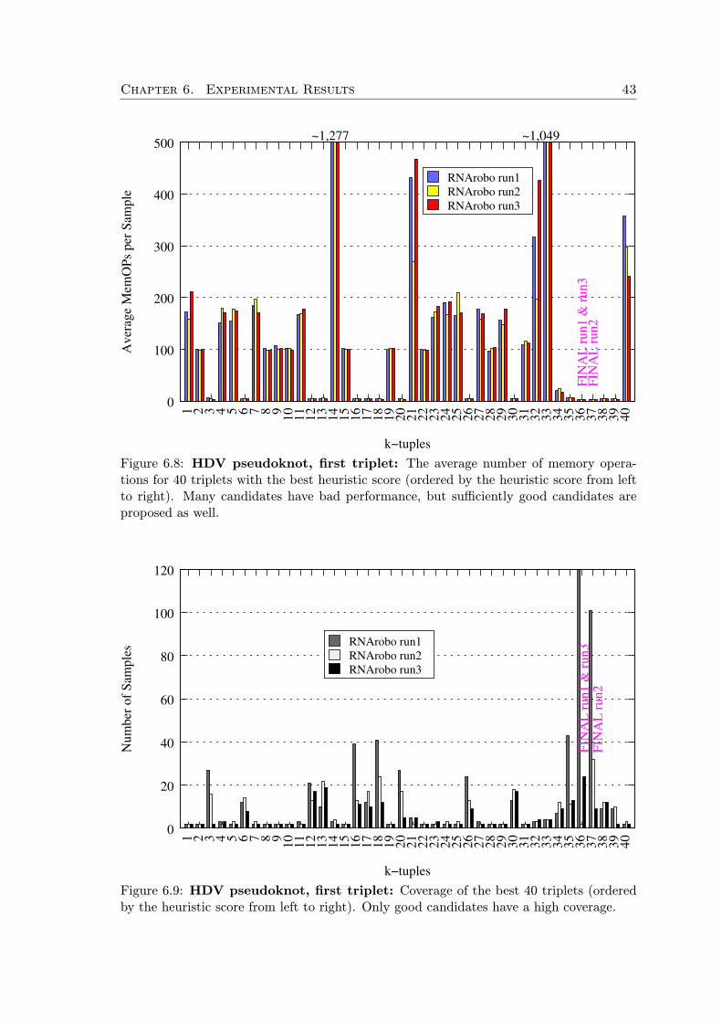
Chapter 6. Experimental Results 43
0
100
200
300
400
500
1 2 3 4 5 6 7 8 91
01
11
21
31
41
51
61
71
81
92
02
12
22
32
42
52
62
72
82
93
03
13
23
33
43
53
63
73
83
94
0
Av
erag
e M
emO
Ps
per
Sam
ple
k−tuples
~1,277 ~1,049
FIN
AL
ru
n1
& r
un
3F
INA
L r
un
2
RNArobo run1
RNArobo run2
RNArobo run3
Figure 6.8: HDV pseudoknot, first triplet: The average number of memory opera-tions for 40 triplets with the best heuristic score (ordered by the heuristic score from leftto right). Many candidates have bad performance, but sufficiently good candidates areproposed as well.
0
20
40
60
80
100
120
1 2 3 4 5 6 7 8 91
01
11
21
31
41
51
61
71
81
92
02
12
22
32
42
52
62
72
82
93
03
13
23
33
43
53
63
73
83
94
0
Nu
mb
er o
f S
amp
les
k−tuples
FIN
AL
ru
n1
& r
un
3F
INA
L r
un
2
RNArobo run1
RNArobo run2
RNArobo run3
Figure 6.9: HDV pseudoknot, first triplet: Coverage of the best 40 triplets (orderedby the heuristic score from left to right). Only good candidates have a high coverage.

Chapter 6. Experimental Results 44
0.0
0.5
1.0
1.5
2.0
2.5
3.0
3.5
4.0
4.5
5.0
1 2 3 4 5 6 7 8 91
01
11
21
31
41
51
61
71
81
92
02
12
22
32
42
52
62
72
82
93
03
13
23
33
43
53
63
73
83
94
0
Av
erag
e M
emO
Ps
per
Sam
ple
k−tuples
FIN
AL
ru
n1
& r
un
3
RNArobo run1
RNArobo run3
Figure 6.10: HDV pseudoknot, second triplet in run1 & run3: The average numberof memory operations for 40 triplets with the best heuristic score (ordered by the heuristicscore from left to right).
0
20
40
60
80
100
120
1 2 3 4 5 6 7 8 91
01
11
21
31
41
51
61
71
81
92
02
12
22
32
42
52
62
72
82
93
03
13
23
33
43
53
63
73
83
94
0
Nu
mb
er o
f S
amp
les
k−tuples
RNArobo run1
RNArobo run3
Figure 6.11: HDV pseudoknot, second triplet in run1 & run3: Coverage of thebest 40 triplets (ordered by the heuristic score from left to right).
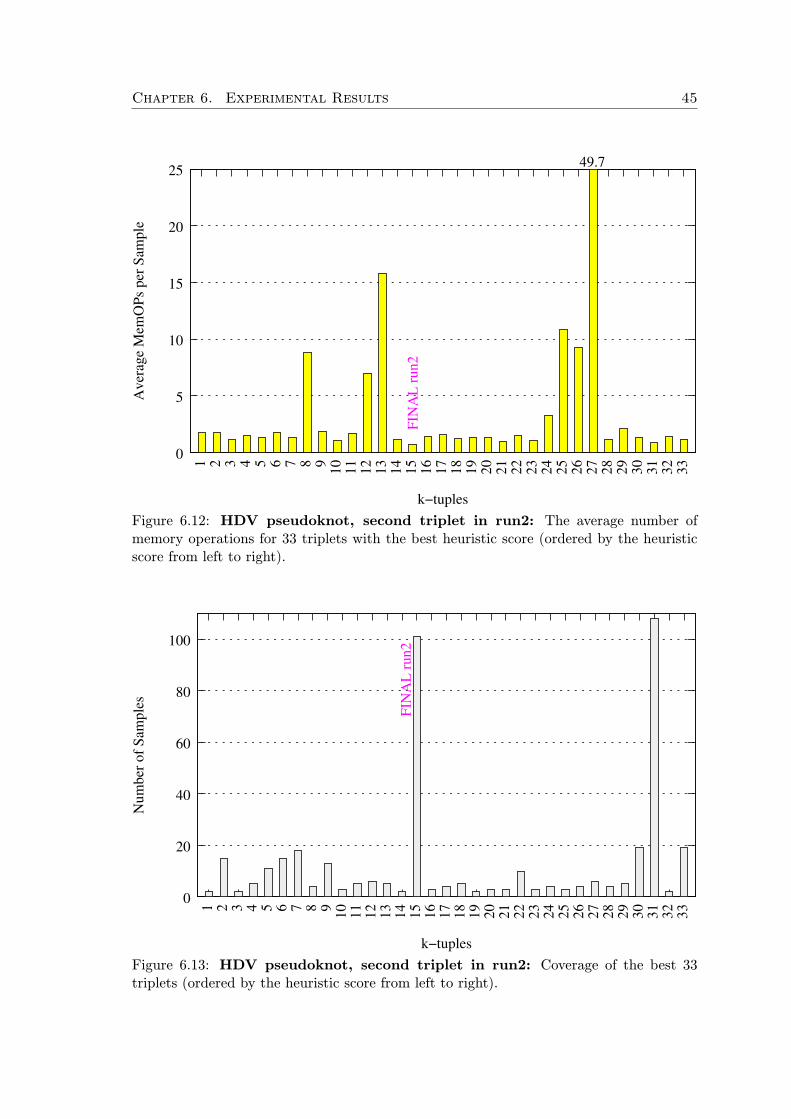
Chapter 6. Experimental Results 45
0
5
10
15
20
25
1 2 3 4 5 6 7 8 91
01
11
21
31
41
51
61
71
81
92
02
12
22
32
42
52
62
72
82
93
03
13
23
3
Av
erag
e M
emO
Ps
per
Sam
ple
k−tuples
49.7
FIN
AL
ru
n2
Figure 6.12: HDV pseudoknot, second triplet in run2: The average number ofmemory operations for 33 triplets with the best heuristic score (ordered by the heuristicscore from left to right).
0
20
40
60
80
100
1 2 3 4 5 6 7 8 91
01
11
21
31
41
51
61
71
81
92
02
12
22
32
42
52
62
72
82
93
03
13
23
3
Nu
mb
er o
f S
amp
les
k−tuples
FIN
AL
ru
n2
Figure 6.13: HDV pseudoknot, second triplet in run2: Coverage of the best 33triplets (ordered by the heuristic score from left to right).

Chapter 6. Experimental Results 46
0
500
1,000
1,500
2,000
2,500
3,000
1 2 3 4 5 6 7 8 91
01
11
21
31
41
51
61
71
81
92
02
12
22
32
42
52
62
72
82
93
03
13
23
33
43
53
63
73
83
94
0
Av
erag
e M
emO
Ps
per
Sam
ple
k−tuples
FIN
AL
ru
n1
& r
un
3
FIN
AL
ru
n2
~6,386 ~6,160 ~7,016 ~6,316
RNArobo run1
RNArobo run2
RNArobo run3
Figure 6.14: HH ribozyme, first triplet: The average number of memory operationsfor 40 triplets with the best heuristic score (ordered by the heuristic score from left toright). Four of the candidates perform really inferior, however there is also many goodcandidates.
0
10
20
30
40
50
60
70
80
1 2 3 4 5 6 7 8 91
01
11
21
31
41
51
61
71
81
92
02
12
22
32
42
52
62
72
82
93
03
13
23
33
43
53
63
73
83
94
0
Nu
mb
er o
f S
amp
les
k−tuples
FIN
AL
ru
n1
& r
un
3
FIN
AL
ru
n2
RNArobo run1
RNArobo run2
RNArobo run3
Figure 6.15: HH ribozyme, first triplet: Coverage of the best 40 triplets (ordered bythe heuristic score from left to right).
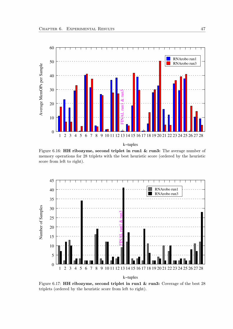
Chapter 6. Experimental Results 47
0
10
20
30
40
50
60
1 2 3 4 5 6 7 8 9 10 11 12 13 14 15 16 17 18 19 20 21 22 23 24 25 26 27 28
Av
erag
e M
emO
Ps
per
Sam
ple
k−tuples
FIN
AL
ru
n1
& r
un
3
RNArobo run1
RNArobo run3
Figure 6.16: HH ribozyme, second triplet in run1 & run3: The average number ofmemory operations for 28 triplets with the best heuristic score (ordered by the heuristicscore from left to right).
0
5
10
15
20
25
30
35
40
45
1 2 3 4 5 6 7 8 9 10 11 12 13 14 15 16 17 18 19 20 21 22 23 24 25 26 27 28
Nu
mb
er o
f S
amp
les
k−tuples
FIN
AL
ru
n1
& r
un
3
RNArobo run1
RNArobo run3
Figure 6.17: HH ribozyme, second triplet in run1 & run3: Coverage of the best 28triplets (ordered by the heuristic score from left to right).

Chapter 6. Experimental Results 48
0
10
20
30
40
50
60
1 2 3 4 5 6 7 8 91
01
11
21
31
41
51
61
71
81
92
02
12
22
32
42
52
62
72
82
93
03
13
23
33
43
53
63
73
83
94
0
Av
erag
e M
emO
Ps
per
Sam
ple
k−tuples
FIN
AL
ru
n2
Figure 6.18: HH ribozyme, second triplet in run2: The average number of memoryoperations for 40 triplets with the best heuristic score (ordered by the heuristic score fromleft to right).
0
20
40
60
80
100
120
140
1 2 3 4 5 6 7 8 91
01
11
21
31
41
51
61
71
81
92
02
12
22
32
42
52
62
72
82
93
03
13
23
33
43
53
63
73
83
94
0
Nu
mb
er o
f S
amp
les
k−tuples
FIN
AL
ru
n2
Figure 6.19: HH ribozyme, second triplet in run2: Coverage of the best 40 triplets(ordered by the heuristic score from left to right).

Chapter 6. Experimental Results 49
0
100
200
300
400
500
600
700
800
1 2 3 4 5 6 7 8 91
01
11
21
31
41
51
61
71
81
92
02
12
22
32
42
52
62
72
82
93
03
13
23
33
43
53
63
73
83
94
0
Av
erag
e M
emO
Ps
per
Sam
ple
k−tuples
FIN
AL
ru
n1
& r
un
2 &
ru
n3
RNArobo run1
RNArobo run2
RNArobo run3
Figure 6.20: tRNA, first triplet: The average number of memory operations for 40triplets with the best heuristic score (ordered by the heuristic score from left to right).
0
20
40
60
80
100
120
1 2 3 4 5 6 7 8 91
01
11
21
31
41
51
61
71
81
92
02
12
22
32
42
52
62
72
82
93
03
13
23
33
43
53
63
73
83
94
0
Nu
mb
er o
f S
amp
les
k−tuples
FIN
AL
ru
n1
& r
un
2 &
ru
n3
RNArobo run1
RNArobo run2
RNArobo run3
Figure 6.21: tRNA, first triplet: Coverage of the best 40 triplets (ordered by theheuristic score from left to right).

Chapter 6. Experimental Results 50
0
2
4
6
8
101 2 3 4 5 6 7 8 9
10
11
12
13
14
15
16
17
18
19
20
21
22
23
24
25
26
27
28
29
30
31
32
33
34
35
36
Av
erag
e M
emO
Ps
per
Sam
ple
k−tuples
FIN
AL
ru
n2
FIN
AL
ru
n1
& r
un
3
RNArobo run1
RNArobo run2
RNArobo run3
Figure 6.22: tRNA, second triplet: The average number of memory operations for 36triplets with the best heuristic score (ordered by the heuristic score from left to right).
0
20
40
60
80
100
120
1 2 3 4 5 6 7 8 91
01
11
21
31
41
51
61
71
81
92
02
12
22
32
42
52
62
72
82
93
03
13
23
33
43
53
6
Nu
mb
er o
f S
amp
les
k−tuples
FIN
AL
ru
n2
FIN
AL
ru
n1
& r
un
3
RNArobo run1
RNArobo run2
RNArobo run3
Figure 6.23: tRNA, second triplet: Coverage of the best 36 triplets (ordered by theheuristic score from left to right).
Conclusion
In this work we studied the problem of RNA structural motif search from two aspects.Firstly, we studied its computational complexity. Secondly, we enhanced our previoustool [Rampášek, 2010] to be a practical solution for this problem even in large genomicdatasets. The main advantage of our tool RNArobo is the ability to search for arbitrarilypseudoknotted motifs with insertions, which we handle in a unique way. In the last partof our work, under the guidance of prof. Andrej Lupták, we developed an in silico methodfor post-processing of the RNArobo search results according to their estimated structuralstability.
In the first part of the thesis, we devoted our attention to the study of computationalcomplexity of RNA structural motif search problem (RNA-SMS). We formally defineda generalized problem, the structural motif search problem (SMS), and proved it to beNP-complete. The proof was conducted by a reduction from another NP-complete prob-lem, ONE-IN-THREE 3SAT. We subsequently showed a straightforward modification ofthe reduction to obtain NP-completeness of RNA-SMS. In our study, we also identifiedtwo causes of the NP-completeness: elements of variable length, and pseudoknots in theirgeneral form. In further work, we would like to investigate, whether some weaker restric-tions on one of these properties would enable us to device an efficient search algorithm.Examples might include limited number of pseudoknots or limits on their relative posi-tion (e.g. planar pseudoknots). Restricting pseudoknots in some way in return for effi-cient algorithm has already been studied for RNA secondary structure prediction problem[Crochemore et al., 2005, Rivas and Eddy, 1999], however not for RNA structural motifsearch.
Proving RNA-SMS to be NP-complete diminished our hopes for a general solution indeterministic polynomial time. Thus, we have worked to improve our previously proposedRNArobo algorithm to shorten its execution time in practice. RNArobo is a backtrackingbased algorithm, and as such, it is sensitive to ordering of variables (elements). We pro-posed a data-driven method for finding a close-to-optimal element ordering. Our methodproved to be significantly beneficial in multiple experimental tests. For complex motifs theimplementation of RNArobo with this method tends to perform faster than the establishedtools. This is especially true for pseudoknotted motifs, and for motifs with many alloweddistortions, when RNArobo benefits from its robustness. On the other hand, when a motifdoes not allow for distortions, our dynamic programming is not as efficient as the methodsused in the other tools. Thus in future, we would like to further enhance RNArobo timeperformance. One possible way would be to augment RNArobo by a pre-filtering tech-nique, such that we could quickly filter out large portions of the searched database. This
51

Conclusion 52
would allow us to focus only on those parts, which exhibit some evidence of a possiblemotif occurrence.
The third contribution of our work is a set of tools for RNArobo result evaluation.These tools automate the analysis which a biochemist expert would do manually, thusfacilitating a high-throughput post-processing of results.
Overall our work resulted in a practical computational pipeline, similar to that pro-posed in [Jimenez et al., 2012], that can be used to discover new homologs of functionalRNAs.

Appendix A
The IUPAC Notation
Symbol Meaning Mnemonic
DNA Bases A Adenosine AdenosineC Cytosine CytosineG Guanine GuanineT Thymine Thymine
Ambiguity Characters R G + A puRineY T + C pYrimidineS G + C Strong interactions (3H bonds)W T + A Weak interactions (2H bonds)K G + T KetoM A + C aMinoD G + T + A Not-C (D follows C in alphabet)H T + A + C Not-G (H follows G)B G + T + C Not-B (B follows A)V G + A + C Not-T or U (V follows U)N G + A + T + C aNy
Table A.1: The IPUAC nucleic acid notation
53

Appendix B
Motif Descriptors
� �# ATP aptamer#
h1 r2 s1 r3 h4 s2 h4’ r3’ s3 r2’ h1’
h1 0:0 *****:*****r2 0:0 NNNN:NNNN TGCAr3 0:0 CNNN:NNNG TGCAh4 0:0 *****:*****
s1 0 GGAAGAAACTGs2 0 NNN[17]s3 0 G� �
Listing B.1: Descriptor for ATP aptamer [Lupták, 2011]
� �# HDV pseudoknot#
h1 r2 s1 r3 s2 r4 r5 s3 r5’ r2’ h1’ s4 h6 s5 h6’ s6 r3’ r4’
h1 0:0 R:Yr2 0:1 NNNNNN:NNNNNN TGCAr3 0:0 NNNN**:**NNNN TGCAr4 0:0 NNN:NNN TGCAr5 0:0 NNN:NNN TGCAh6 0:1 NNNN****:****NNNN
s1 0 N[14]s2 0 *s3 0 TNCNCGY*s4 0 GN****s5 0 NNN[20]s6 0 CNRA*� �
Listing B.2: Descriptor for HDV pseudoknot [Lupták, 2011]
54

Appendix B. Motif Descriptors 55
� �# Hammerhead Ribozyme#
s1 r1 s2 r2 s3 r2’ s4 r3 s5 r3’ s6 r1’ s7
r1 0:0 ***NNN:NNN*** TGCAr2 0:0 ***NNN:NNN*** TGCAr3 0:0 ***NNN:NNN*** TGCA
s1 0 NNNNNNNNNNs2 0 CTGANGAs3 0 NNNN[46]s4 0 GAAAs5 0 NNNN[46]s6 0 TNs7 0 NNNNNNNNNN� �
Listing B.3: Descriptor for Hammerhead Ribozyme [Lupták, 2011]
� �# tRNA#
h1 s1 h2 s2 h2’ s3 h3 s4 h3’ s5 h4 s6 h4’ h1’ s8
h1 0:2 NNNNNNN:NNNNNNNh2 0:1 *NNN:NNN*h3 0:1 NNNNN:NNNNNh4 0:1 NNNNN:NNNNNs1 0 TNs2 0 NNNN**********s3 0 Ns4 0 NNNNNN*s5 0 NN********************s6 0 TTC****s8 0 NCCA� �
Listing B.4: Descriptor for tRNA [Eddy, 1996]

Bibliography
[Bellaousov and Mathews, 2010] Bellaousov, S. and Mathews, D. (2010). ProbKnot: Fastprediction of RNA secondary structure including pseudoknots. RNA, 16(10):1870–1880.
[Billoud et al., 1996] Billoud, B., Kontic, M., and Viari, A. (1996). Palingol: a declara-tive programming language to describe nucleic acids’ secondary structures and to scansequence database. Nucleic Acids Research, 24(8):1395.
[Chang et al., 2006] Chang, T.-H., Huang, H.-D., Chuang, T.-N., Shien, D.-M., andHorng, J.-T. (2006). RNAMST: efficient and flexible approach for identifying RNAstructural homologs. Nucl. Acids Res., 34:W423–428.
[Crochemore et al., 2005] Crochemore, M., Hermelin, D., Landau, G., and Vialette, S.(2005). Approximating the 2-interval pattern problem. Algorithms–ESA 2005, pages426–437.
[Durbin et al., 1998] Durbin, R., Eddy, S., Krogh, A., and Mitchison, G. (1998). Biolog-ical sequence analysis: Probabilistic models of proteins and nucleic acids. CambridgeUniversity Press.
[Eddy, 1996] Eddy, S. (1996). RNABob: a program to search for RNA secondary structuremotifs in sequence databases. unpublished.
[Gautheret et al., 1990] Gautheret, D., Major, F., and Cedergren, R. (1990). Patternsearching/alignment with RNA primary and secondary structures: an effective descrip-tor for tRNA. Comput Appl Biosci, 6(4):325–31.
[George and Tenenbaum, 2009] George, A. D. and Tenenbaum, S. A. (2009). Infor-matic resources for identifying and annotating structural RNA motifs. Mol Biotechnol,41(2):180–93.
[Grillo et al., 2003] Grillo, G., Licciulli, F., Liuni, S., Sbisa, E., and Pesole, G. (2003).PatSearch: a program for the detection of patterns and structural motifs in nucleotidesequences. Nucleic Acids Research, 31(13):3608.
[Hofacker et al., 1994] Hofacker, I., Fontana, W., Stadler, P., Bonhoeffer, L., Tacker, M.,and Schuster, P. (1994). Fast folding and comparison of RNA secondary structures.Monatshefte für Chemie/Chemical Monthly, 125(2):167–188.
56
Bibliography 57
[Jimenez et al., 2012] Jimenez, R., Rampášek, L., Brejová, B., Vinař, T., and Lupták, A.(2012). Discovery of rna motifs using a computational pipeline that allows insertionsin paired regions and filtering of candidate sequences. Methods in molecular biology(Clifton, NJ), 848:145.
[Kim and Cohen, 1998] Kim, S. and Cohen, A. (1998). On the Behrens-Fisher problem:A review. Journal of Educational and Behavioral Statistics, 23(4):356–377.
[Lathrop, 1994] Lathrop, R. (1994). The protein threading problem with sequence aminoacid interaction preferences is NP-complete. Protein Engineering Design and Selection,7(9):1059.
[Lorenz et al., 2011] Lorenz, R., Bernhart, S., zu Siederdissen, C., Tafer, H., Flamm, C.,Stadler, P., and Hofacker, I. (2011). ViennaRNA package 2.0. Algorithms for MolecularBiology, 6(1):26.
[Lowe and Eddy, 1997] Lowe, T. and Eddy, S. (1997). tRNAscan-SE: a program for im-proved detection of transfer RNA genes in genomic sequence. Nucleic acids research,25(5):0955–964.
[Lupták, 2011] Lupták, A. (2011). personal communication.
[Lyngsø, 2004] Lyngsø, R. (2004). Complexity of pseudoknot prediction in simple models.Automata, Languages and Programming, pages 171–211.
[Macke et al., 2001] Macke, T. J., Ecker, D. J., Gutell, R. R., Gautheret, D., Case, D. A.,and Sampath, R. (2001). RNAMotif, an RNA secondary structure definition and searchalgorithm. Nucl. Acids Res., 29(22):4724–4735.
[McCaskill, 1990] McCaskill, J. (1990). The equilibrium partition function and base pairbinding probabilities for RNA secondary structure. Biopolymers, 29(6-7):1105–1119.
[NCBI, 2012a] NCBI (2012a). National Center for Biotechnology Information database:genome of Drosophila melanogaster. ”ftp://ftp.ncbi.nlm.nih.gov/genomes/Drosophila_melanogaster/”.
[NCBI, 2012b] NCBI (2012b). National Center for Biotechnology Informationdatabase: genome of Homo sapiens. ”ftp://ftp.ncbi.nlm.nih.gov/genomes/H_sapiens/”.
[Nussinov and Jacobson, 1980] Nussinov, R. and Jacobson, A. (1980). Fast algorithm forpredicting the secondary structure of single-stranded RNA. Proceedings of the NationalAcademy of Sciences, 77(11):6309.
[Rampášek, 2010] Rampášek, L. (2010). RNA motif search in genomic sequences. Bach-elor thesis, Faculty of Mathematics, Physics and Informatics, Comenius University inBratislava.

Bibliography 58
[Rampášek, 2011] Rampášek, L. (2011). RNA structural motif search is NP-complete.Proceedings of the Student Science Conference 2011, Faculty of Mathematics, Physicsand Informatics, Comenius University in Bratislava.
[Reeder et al., 2007] Reeder, J., Reeder, J., and Giegerich, R. (2007). Locomotif: fromgraphical motif description to RNA motif search. Bioinformatics, 23(13):i392–i400.
[Ren et al., 2005] Ren, J., Rastegari, B., Condon, A., and Hoos, H. (2005). Hot-Knots: heuristic prediction of RNA secondary structures including pseudoknots. Rna,11(10):1494–1504.
[Rivas and Eddy, 1999] Rivas, E. and Eddy, S. (1999). A dynamic programming algorithmfor RNA structure prediction including pseudoknots1. Journal of molecular biology,285(5):2053–2068.
[Ruminski et al., 2010] Ruminski, D., Webb, C., Riccitelli, N., and Luptak, A. (2010).Processing of insect retrotransposons by self-cleaving ribozymes.
[Russell and Norvig, 2010] Russell, S. and Norvig, P. (2010). Artificial intelligence: Amodern approach. Prentice hall.
[Ruxton, 2006] Ruxton, G. (2006). The unequal variance t-test is an underused alternativeto Student’s t-test and the Mann–Whitney U test. Behavioral Ecology, 17(4):688–690.
[Sato et al., 2011] Sato, K., Kato, Y., Hamada, M., Akutsu, T., and Asai, K. (2011).IPknot: fast and accurate prediction of RNA secondary structures with pseudoknotsusing integer programming. Bioinformatics, 27(13):i85–i93.
[Satterthwaite, 1946] Satterthwaite, F. (1946). An approximate distribution of estimatesof variance components. Biometrics bulletin, 2(6):110–114.
[Schaefer, 1978] Schaefer, T. (1978). The complexity of satisfiability problems. In Pro-ceedings of the tenth annual ACM symposium on Theory of computing, pages 216–226.ACM.
[Smith, 1936] Smith, H. (1936). The problem of comparing the results of two experimentswith unequal errors. Journal of the Council of Scientific and Industrial Research, 9:211–212.
[Sperschneider and Datta, 2010] Sperschneider, J. and Datta, A. (2010). DotKnot: pseu-doknot prediction using the probability dot plot under a refined energy model. Nucleicacids research, 38(7):e103–e103.
[Webb et al., 2009] Webb, C. H., Riccitelli, N. J., Ruminski, D. J., and Luptak, A. (2009).Widespread occurrence of self-cleaving ribozymes. Science, 326(5955):953.
[Welch, 1947] Welch, B. (1947). The generalization of ‘Student’s’ problem when severaldifferent population variances are involved. Biometrika, 34(1/2):28–35.

Bibliography 59
[Xayaphoummine et al., 2005] Xayaphoummine, A., Bucher, T., and Isambert, H. (2005).Kinefold web server for RNA/DNA folding path and structure prediction includingpseudoknots and knots. Nucleic acids research, 33(suppl 2):W605–W610.
[Zuker and Sankoff, 1984] Zuker, M. and Sankoff, D. (1984). RNA secondary structuresand their prediction. Bulletin of Mathematical Biology, 46(4):591–621.