computational aspects of a new multi-scale...

This is a repository copy of Computational aspects of a new multi-scale dispersive gradient elasticity model with micro-inertia.

White Rose Research Online URL for this paper:http://eprints.whiterose.ac.uk/103176/

Version: Accepted Version

Article:

De domenico, D. and Askes, H. orcid.org/0000-0002-4900-1376 (2016) Computational aspects of a new multi-scale dispersive gradient elasticity model with micro-inertia. International Journal for Numerical Methods in Engineering. ISSN 0029-5981

https://doi.org/10.1002/nme.5278

This is the peer reviewed version of the following article: De Domenico, D., and Askes, H. (2016) Computational aspects of a new multi-scale dispersive gradient elasticity model with micro-inertia. Int. J. Numer. Meth. Engng, which has been published in final form at http://onlinelibrary.wiley.com/doi/10.1002/nme.5278. This article may be used for non-commercial purposes in accordance with Wiley Terms and Conditions for Self-Archiving

[email protected]://eprints.whiterose.ac.uk/

Reuse

Unless indicated otherwise, fulltext items are protected by copyright with all rights reserved. The copyright exception in section 29 of the Copyright, Designs and Patents Act 1988 allows the making of a single copy solely for the purpose of non-commercial research or private study within the limits of fair dealing. The publisher or other rights-holder may allow further reproduction and re-use of this version - refer to the White Rose Research Online record for this item. Where records identify the publisher as the copyright holder, users can verify any specific terms of use on the publisher’s website.

Takedown

If you consider content in White Rose Research Online to be in breach of UK law, please notify us by emailing [email protected] including the URL of the record and the reason for the withdrawal request.

mailto:[email protected]

https://eprints.whiterose.ac.uk/

INTERNATIONAL JOURNAL FOR NUMERICAL METHODS IN ENGINEERINGInt. J. Numer. Meth. Engng 2010; 00:1–21Published online in Wiley InterScience (www.interscience.wiley.com). DOI: 10.1002/nme

Computational aspects of a new multi-scale dispersive gradientelasticity model with micro-inertia

Dario De Domenico 1∗, Harm Askes 2

1 Department PAU, University Mediterranea of Reggio Calabria, via Melissari, Reggio Calabria 89124, Italy2 Department of Civil and Structural Engineering, University of Sheffield, Mappin Street, Sheffield S1 3JD, UK

SUMMARY

Computational aspects of a recently developed gradient elasticity model are discussed in this paper. Thismodel includes the (Aifantis) strain gradient term along with two higher-order acceleration terms (micro-inertia contributions). It has been demonstrated that the presence of these three gradient terms enables oneto capture the dispersive wave propagation with great accuracy. In this paper, the discretisation details ofthis model are thoroughly investigated, including both discretisation in time and in space. Firstly, the criticaltime step is derived that is relevant for conditionally stable time integrators. Secondly, recommendations onhow to choose the numerical parameters, primarily the element size and time step, are given by comparingthe dispersion behaviour of the original higher-order continuum with that of the discretised medium. In sodoing, the accuracy of the discretised model can be assessed a priori depending on the selected discretisationparameters for given length scales. A set of guidelines can therefore be established to select optimaldiscretisation parameters that balance computational efficiency and numerical accuracy. These guidelinesare then verified numerically by examining the wave propagation in a one-dimensional bar as well as in atwo-dimensional example.Copyright c© 2010 John Wiley & Sons, Ltd.

Received . . .

KEY WORDS: Wave dispersion; Gradient elasticity; Multiscale; Finite element methods; Dynamicalsystems; Generalised continuum

1. INTRODUCTION

Constitutive elastic models for classical continuous media yield a local description of the problem

fields whereby the stress at a point depends uniquely upon the strain at that point. Such local-

type models are consistent with the underlying assumption that the external length-scales and time-

scales are much larger than the those of the dominant heterogeneities. Consequently, classical (local)

elasticity theory fails to capture phenomena where nonlocal interactions affect the problem outcome,

for example at crack-tips or around dislocation cores, for describing size effects, and dispersive wave

propagation.

Focusing the attention on wave dispersion, it is usually found that the velocity of the

harmonic components reduces as wavelengths approach the physical dimension of the underlying

microstructure of a material. These dispersive phenomena cannot be captured unless long-range

interactions occurring within the material micro-structure are accounted for in the constitutive

model. Therefore, an obvious solution could be to take into account nonlocal interactions between

atoms by modelling every single microstructural component individually, which represents the basis

∗Correspondence to: Dario De Domenico, Department PAU, University Mediterranea of Reggio Calabria, ReggioCalabria 89124, Italy. Email: [email protected]

Copyright c© 2010 John Wiley & Sons, Ltd.

Prepared using nmeauth.cls [Version: 2010/05/13 v3.00]

2 D. DE DOMENICO, H. ASKES

of atomistic models. Besides being very difficult to model the exact microstructure for most practical

engineering problems, such models are often computationally prohibitive or extremely demanding

on memory resources and thus unfeasible to deal with real engineering problems. As an alternative,

many enriched (or generalised) continuum theories have been developed to bridge the gap between

atomistic models and classical continuum mechanics theory. These theories equip the continuum

(macrostructural) formulation with additional length- and time-scales that reflect the underlying

material microstructure, see e.g. [2, 4, 7, 12–14, 17, 20] for some comprehensive reviews.

In this paper we restrict our attention to gradient elasticity models, which are a special class of

the above generalised theories [1, 4]. These models extend classical elasticity theory by means of

additional higher-order spatial derivatives of strains, stresses and/or accelerations in the constitutive

equations or in the equations of motion. A class of effective gradient theories for use in dynamics

incorporates mixed spatial-temporal derivatives and contains both higher-order strain gradients and

higher-order inertia terms. The former are useful to remove singularities, the latter are essential

to simulate wave dispersion. The simultaneous presence of both strain gradients and micro-inertia

terms has been denoted as dynamic consistency in certain previous articles [4–6].

The model dealt with in this paper is an extension of an earlier dynamically consistent

model having two gradient contributions [3–5], namely a strain gradient and a micro-inertia term

(acceleration gradient). Compared to the latter model, the proposed ‘enhanced’ model presents a

third gradient contribution, namely an additional micro-inertia term multiplying the fourth-order

space derivative of the acceleration field in the equations of motion. Therefore, the proposed

model incorporates three gradient contributions, which are accompanied by three corresponding

length scales. The formulation and finite element implementation of such model have already been

discussed in [10]. Since the governing partial differential equations are fourth-order in space, spatial

discretisation would require C 1-continuity of the interpolation, i.e. continuity of the displacements

as well as the much more complicated continuity of the displacement derivatives. To avoid this,

the fourth-order equations have been split into a set of two (coupled and symmetric) second-

order equations so that C 0-shape functions are sufficient in the finite element implementation.

Variationally consistent boundary conditions have been derived and the corresponding discretised

equations have been discussed [10]. It has been found that this model is very versatile and provides

an improved dispersion behaviour due to the presence of the additional micro-inertia contribution.

The inclusion of three free parameters in a gradient elasticity formulation enables a very flexible

dispersion curve that can be tailored for a broad variety of engineering materials.

In this paper we do not investigate the physical motivations further but rather we focus on some

computational aspects of this model concerning discretisation in space and in time of the underlying

equations of motion. Firstly, the continuum equations and the discrete equations of the considered

gradient elasticity model are summarised in Section 2. In Section 3 the dispersion relations of the

continuum model for compression and shear waves are derived. Some arguments concerning the

time integration, the use of explicit or implicit time integrators, as well as the adoption of a lumped

or consistent mass matrix formulation are comprised in Section 4. In Section 5 stability aspects are

investigated and it is illustrated how the critical time step in the Newmark time integration is affected

by the three length scale parameters of the model. Accuracy aspects related to the discretisation are

then investigated in Section 6: on the basis of the dispersion analysis of the discretised medium,

some guidelines can be established to select optimal values for the element size h and the time

step ∆t for given length scale parameters. These optimal values can be assessed a priori according

to the desired accuracy of the numerical solution as compared to the continuum counterpart. The

validity of these guidelines is finally scrutinised in Section 7 by means of two numerical examples

concerning the wave propagation in a one-dimensional bar and in a two-dimensional body.

Notation

In the index tensor notation, subscripts denote components with respect to an orthogonal Cartesian

coordinate system, say xi (i = 1, 2, 3); the Einstein summation convention for repeated indices

holds. Spatial derivatives are denoted by the comma notation, that is ui,j = ∂ui/∂xj . A super-

imposed dot denotes the derivative with respect to time, that is ui = ∂ui/∂t. In the matrix-vector

notation, boldface lowercase and capital variables denote vectors and matrices, respectively. The

Copyright c© 2010 John Wiley & Sons, Ltd. Int. J. Numer. Meth. Engng (2010)Prepared using nmeauth.cls DOI: 10.1002/nme

COMPUTATIONAL ASPECTS OF A NEW GRADIENT ELASTICITY MODEL 3

symbol := means equality by definition. Other symbols will be defined in the text at their first

appearance.

2. CONTINUUM EQUATIONS AND SPATIAL DISCRETISATION

Recently, an enhanced gradient elasticity model has been formulated [10]. In this Section we

summarise the governing equations of both the higher-order continuum and the spatially discretised

counterpart. Such model has been devised based on an earlier dynamically consistent model

proposed in [3, 5] and having a strain gradient term as well as a micro-inertia contribution. These

two gradients, related to the second-order space derivative of the strain field and of the acceleration

field, were accompanied by two material parameters characterising the underlying microstructure

and identified as a length scale in statics and in dynamics, respectively.

Motivated by nano-scale experimental evidence on the dispersion characteristics of materials with

a lattice structure [22–24], a third additional higher-order inertia contribution has been incorporated

in the aforementioned enhanced model. It has been found that such additional micro-inertia term

results in a significantly improved dispersion behaviour. Indeed, the associated dispersion curve of

this three-parameter model is very flexible, which makes it easy to to tailor it for a broad variety of

materials so as to achieve a qualitative match with their corresponding experimental curve—see for

instance the simulation of wave propagation in discrete systems and laminates studied in [10].

The model with three parameters formulated in [10] in the hypothesis of homogeneous material

(constant density and stiffness tensor) is defined by the following equations of motion

ρ(

ui − αℓ2ui,nn + βℓ4ui,jjnn

)

= Cijkl

(

uk,jl − γℓ2uk,jlnn

)

(1)

where Cijkl is a fourth-order tensor representing the material stiffness, ui represent the displacement

field and ρ is the mass density. In the sequel we will restrict our attention to isotropic materials for

which Cijkl = λδijδkl + µδikδjl + µδilδjk, δij being Kronecker’s delta and λ, µ the Lame constants.

For reasons of dimensional consistency, in (1) the three gradient terms are accompanied by three

distinct factors related to the length scale ℓ characterising the underlying material microstructure.

The three coefficients α, β, γ adjust the relative magnitudes between the various length scales

appearing in the strain gradient term and in the micro-inertia contributions. The γℓ2-term represents

the gradient enrichment of the one parameter Aifantis 1992 strain gradient theory [1,2,21], whereas

the earlier dynamically consistent model of [3, 5] is captured by the simultaneous presence of the

αℓ2 and γℓ2-terms. Compared to the latter model, an additional term βℓ4 appears in the equations

of motion (1) multiplying the fourth-order space derivative of the acceleration field. Therefore, the

proposed model is defined by three independent parameters that are three length scales representing

the underlying material microstructure. Procedures to link these three constitutive coefficients to

micro-structural properties for a few simple mechanical problems have been discussed in [10].

By inspection of Eq. (1) it emerges that the governing differential equations contains fourth-order

spatial derivatives of the ui unknowns (not only the displacements but also the accelerations). With

regard to numerical implementations, this would require shape functions that are C 1-continuous.

Although this requirement might be met by using Hermitian C 1 finite elements [26], discontinuous

Galerkin methods [11], meshless methods [6] or, alternatively, by discretising multiple fields [25],

a simpler approach has been adopted in [10]. According to the latter approach, the fourth-order

differential equations are recast, via an operator split, into a set of two second-order differential

equations so that a standard finite element implementation with C 0-continuous interpolation

functions suffices. To this aim, an auxiliary variable, identified as the microscopic displacement field

umi , has been introduced in addition to the macroscopic displacement field ui ≡ uM

i entering Eq. (1).

These two displacement fields are related to each other by the differential relation uMi − γℓ2uM

i,nn =umi . The fourth-order differential equations (1) are then rearranged as a set of two coupled and

symmetric second-order differential equations in umi and uM

i as follows (see [10] for the full



derivation)

ρ

[

(

α

γ− β

γ2

)

umi − βℓ2

γumi,nn −

(

α

γ− β

γ2− 1

)

uMi

]

= Cijkl umk,jl (2a)

ρ

[

−(

α

γ− β

γ2− 1

)

umi +

(

α

γ− β

γ2− 1

)

uMi −

(

α− β

γ− γ

)

ℓ2uMi,nn

]

= 0 . (2b)

By virtue of the formulation given by Eqs. (2), the additional β term does not imply any additional

computational cost as compared to the earlier dynamically consistent model (i.e. with regard to the

spatial discretisation and the resulting finite element implementation). The proposed formulation

may therefore be considered as an enhanced version of the earlier dynamically consistent model,

the latter being retrieved for a zero value of the β term.

As regards the finite element implementation of Eqs. (2), discretisation of the micro- and macro-

displacements um and uM is carried out with shape functions Nm and NM , respectively. Then,

the weak form of the equations is considered, integration by parts performed and, finally, the semi-

discretised format of equations (i.e. discretised in space but continuous in time) are obtained as

follows[

M11 −M12

−MT12 M22

] [

dm

dM

]

+

[

K11 0

0 0

] [

dm

dM

]

=

[

fext

0

]

(3)

where dm and dM are the nodal displacements associated to the continuum displacement fields um

and uM , respectively, and the matrix blocks entering expression (3) are defined as

M11 =

∫

Ω

NmT ρ

(

α

γ− β

γ2

)

NmdΩ +∑

ξ=x,y,z

∫

Ω

∂NmT

∂ξρβℓ2

γ

∂Nm

∂ξdΩ (4a)

M12 =

∫

Ω

NmT ρ

(

α

γ− β

γ2− 1

)

NMdΩ (4b)

M22 =

∫

Ω

NMTρ

(

α

γ− β

γ2− 1

)

NMdΩ +∑

ξ=x,y,z

∫

Ω

∂NMT

∂ξρ

(

α− β

γ− γ

)

ℓ2∂NM

∂ξdΩ (4c)

K11 =

∫

Ω

BmTCBmdΩ (4d)

fext =

∫

Γ

NmTt dΓ. (4e)

In expressions (4), Bm = LNm, where L is a differential operator that relates strains and

displacements such that εm = Lum. Moreover, t = [tx, ty, tz]T are the user-prescribed tractions

on the Neumann part Γn of the boundary expressed as t = NT(

CLum + ρ βℓ2

γ∇um

)

, where ∇denotes the gradient operator and the matrix N contains the components of the outward normal

vector n = [nx, ny, nz]T to the boundary Γ; note the non-standard addition to the tractions which

is in line with earlier gradient theories [3, 5]. Due to the symmetric format of Eqs. (2) (i.e. the

coefficient multiplying uMi in (2a) is equal to the coefficient multiplying um

i in (2b)), the system

matrices are symmetric in the corresponding finite element implementation. It can be seen that the

system matrices are also positive-definite provided that α > βγ+ γ. Time integration of Eqs. (3) is

discussed in Section 4.

3. DISPERSION ANALYSIS OF THE CONTINUUM MODEL

In order to analyse the dispersive properties of Eqs. (2), two-dimensional wave propagation is

studied with reference to a plane strain configuration. Both displacement fields umi and uM

i are



expressed in terms of a dilatation potential Φ and a distortion potential Ψ as

umx = Φm

,x +Ψm,y and um

y = Φm,y −Ψm

,x (5a)

uMx = ΦM

,x +ΨM,y and uM

y = ΦM,y −ΨM

,x . (5b)

Substituting expressions (5) into Eqs. (2a) and (2b) one obtains, respectively

[

∂∂x∂∂y

]

ρ[

(

α

γ− β

γ2

)

(Φm − ΦM ) + ΦM − βℓ2

γ(Φm

,xx + Φm,yy)]

− (λ+ 2µ)(Φm,xx +Φm

,yy)

+

[

∂∂y

− ∂∂x

]

ρ[

(

α

γ− β

γ2

)

(Ψm − ΨM ) + ΨM − βℓ2

γ(Ψm

,xx + Ψm,yy)]

− µ (Ψm,xx +Ψm

,yy)

=

[

00

]

(6a)[

∂∂x∂∂y

]

ρ[

(

α

γ− β

γ2− 1

)

(ΦM − Φm)−(

α− β

γ− γ

)

ℓ2(ΦM,xx + ΦM

,yy)]

+

[

∂∂y

− ∂∂x

]

ρ[

(

α

γ− β

γ2− 1

)

(ΨM − Ψm)−(

α− β

γ− γ

)

ℓ2 (ΨM,xx + ΨM

,yy)]

=

[

00

]

(6b)

Since Eqs. (6) must hold for arbitrary (non-zero) waves, it follows that the expressions in braces

must vanish. Therefore, compressive waves are studied in terms of the dilatation potentials Φm and

ΦM via the following equations

ρ[

(

α

γ− β

γ2

)

(Φm − ΦM ) + ΦM − βℓ2

γ(Φm

,xx + Φm,yy)]

− (λ+ 2µ)(Φm,xx +Φm

,yy) = 0 (7a)

ρ[

(

α

γ− β

γ2− 1

)

(ΦM − Φm)−(

α− β

γ− γ

)

ℓ2(ΦM,xx + ΦM

,yy)]

= 0 (7b)

Since all the model parameters, including the three coefficients characterising the length scale terms

as well as the Lame constants, are assumed to be constant coefficients, Eqs. (7) admit solutions

given by two general harmonic functions

Φm(x, t) = Φm exp(i (kxx+ kyy − ωt)) (8a)

ΦM (x, t) = ΦM exp(i (kxx+ kyy − ωt)) (8b)

where Φm and ΦM are amplitudes, i the imaginary unit, ω the angular frequency whilst kx and kyare the wave numbers in the x and y direction. Substituting these two trial functions into Eqs. (7)

yields

ω2

(

α

γ− β

γ2− 1

)

ΦM + Φm

[

c2pk2 − ω2

(

α

γ− β

γ2(1− γk2ℓ2)

)]

= 0 (9a)

(

α

γ− β

γ2− 1

)

(

Φm − ΦM (1 + γk2ℓ2))

ω2 = 0 (9b)

in which k =√

k2x + k2y represents the modulus of the wave vector in two dimensions and cp =√

(λ+ 2µ)/ρ is the long wave length limit of the compressive wave velocity. From Eq. (9b) one

obtains a relation between the two amplitudes as ΦM = Φm/(1 + γk2ℓ2). Eq. (9a) can then be

elaborated as

Φm

[

ω2

(

α

γ− β

γ2− 1

)

1

1 + γk2ℓ2+ c2pk

2 − ω2

(

α

γ− β

γ2(1− γk2ℓ2)

)]

= 0 (10)

that can be rewritten in dimensionless form by introducing the dimensionless wave number χ := kℓ

c2

c2p=

1 + γχ2

1 + αχ2 + βχ4. (11)



For the shear waves the same procedure is employed with reference to the distortion potentials Ψm

and ΨM in (6), and the following expression is found

c2

c2s=

1 + γχ2

1 + αχ2 + βχ4(12)

where cs =√

µ/ρ is the velocity of the shear waves with infinite wavelength. The comparison

betweens Eqs. (11) and (12) shows that the dispersion curves for the compressive and shear waves

have the same shape, the only difference being the constant by which they are scaled. The dispersion

relations (11) and (12) are such that the strain gradient term accelerates while the micro-inertia

terms decelerate the higher wave numbers compared to the lower wave numbers. Consequently,

for α > γ − βχ2 the higher wave numbers travel slower than the lower wave numbers. The one-

dimensional case may be retrieved from Eq. (11) for a zero value of the Poisson’s ratio ν, leading

to Lame constants λ = 0, µ = E/2 (E being the Young’s modulus) and, thus, cp ≡ ce =√

E/ρwhere ce represents the one-dimensional bar velocity of classical elasticity. Note that unlike the

dynamically consistent model with two length scale parameters [3, 5, 9], the case α = γ does not

lead to a non-dispersive medium due to the presence of the β term in the denominator of Eqs. (11)

and (12).

4. TIME INTEGRATION AND MASS MATRIX FORMULATION ARGUMENTS

Equations (3) are discretised in space but still continuous in time. For the time discretisation of

Eqs. (3) one of the most widely used family of implicit methods is the Newmark family [15, 18].

As well known, if a constant time step ∆t is considered such that two subsequent time instants are

denoted as tj = j∆t and tj+1 = (j + 1)∆t, the (numerical approximation of the) nodal velocities

and nodal displacements at time tj+1 are expressed as

d(j+1) = d(j) +∆t[

(1− γn) d(j) + γn d

(j+1)]

(13a)

d(j+1) = d(j) +∆t d(j) +∆t2

2

[

(1− 2βn) d(j) + 2βnd

(j+1)]

(13b)

where the Newmark parameters γn and βn set the accuracy, stability and numerical damping

of the time integration scheme. The Newmark method is unconditionally stable if γn ≥ 1/2and βn ≥ 1/4 (γn + 1/2)2. The Newmark family contains as special cases many well-known

and widely used methods, for instance the unconditionally stable constant average acceleration

variant (trapezoidal rule) is retrieved for γn = 1/2 and βn = 1/4. Other well-known members of

the Newmark family are the linear acceleration scheme (γn = 1/2 and βn = 1/6) and the Fox-

Goodwin scheme (γn = 1/2 and βn = 1/12), which are only conditionally stable. Stability of the

conditionally stable algorithms is discussed in Section 5.

Due to the structure of the spatially discretised system of equations (3), it is more convenient to

solve in terms of accelerations. The time-discretised counterpart of Eqs. (3) according to expressions

(13) reads[

M11 + βn∆t2 K11 −M12

−MT12 M22

] [

dm(j+1)

dM(j+1)

]

=

[

f(j+1)ext − f

(j)int

0

]

(14)

with

f(j)int = K11

(

dm(j) +∆t dm(j) +∆t2

2(1− 2βn) d

m(j)

)

(15)

which is used for the subsequent simulations in a recursive fashion.

As an alternative, an explicit Runge-Kutta algorithm may be adopted. We consider a vector

d = [dm,dM ]T collecting the microscopic and macroscopic displacements so that Eqs. (3) can be

expressed in compact form as

Md(t) +Kd(t) = F(t). (16)



These n second-order differential equations are recast into a set of 2n first-order equations as follows

y(t) = DN y(t) +VN F(t) (17)

where

y =

[

d

d

]

; DN =

[

0 I

−M−1K 0

]

; VN =

[

0

M−1

]

(18)

0 and I being a n-by-n zero and identity matrices, respectively. Eq. (16) can be handled by explicit

Runge-Kutta solvers implemented as software toolbox, e.g. in MATLAB [16].

It is well known that explicit time integration is efficient if the mass matrix is diagonal. However,

in line with the arguments of Bennett & Askes [9], the use of a lumped mass matrix is not

recommended as this would eliminate all the higher-order effects and would be inappropriate for

this format of gradient elasticity. For this reason, consistent mass matrices will be adopted for all

the numerical examples in the paper.

5. STABILITY ASPECTS: CRITICAL TIME STEP

Some implicit algorithms of the Newmark family are only conditionally stable. Consequently,

the applied time step must be selected smaller than a so-called critical time step in order for the

simulations to remain numerically stable. The critical time step can be calculated as [15]

∆tcrit =Ωcrit

ωmax

(19)

in which Ωcrit is the critical sampling frequency of the Newmark scheme and ωmax is the highest

frequency of the total system. A conservative value of the critical time step is evaluated by taking

an upper bound of the frequency as ωmax = ωemax (where ωe

max is the maximum frequency of

the individual finite element) in combination with a lower bound of the sampling frequency as

Ωcrit = 1/√

γn/2− βn. The maximum frequency that can be captured by the spatial discretisation

depends on the specific element being used (interpolation, type of integration, mass distribution). It

can be obtained by solving the homogeneous equivalent expression of Eqs. (16) at element level,

which yields the following eigenvalue problem in ω

det[−ω2 M+K] = 0. (20)

For a two-noded bar element of length h, unitary cross-section and linear shape functions, the

element mass matrix and stiffness matrix are given by (cf. Eqs. (3) and (4))

M =

(

αγ− β

γ2

)

Mc +βℓ2

γMg −

(

αγ− β

γ2 − 1)

Mc

−(

αγ− β

γ2 − 1)

Mc

(

αγ− β

γ2 − 1)(

Mc + γℓ2 Mg

)

, K =

[

Kc 0

0 0

]

(21)

where Mc and Kc are the usual mass matrix and stiffness matrix of classical elasticity, while Mg is

a gradient-enriched contribution to the mass matrix given by

Mc =ρh

6

[

2 11 2

]

, Kc =E

h

[

1 −1−1 1

]

, Mg =ρ

h

[

1 −1−1 1

]

. (22)

Inserting these expression into the eigenvalue problem (20) leads to three zero eigenvalues

(characterising some rigid body motions) and a non-zero frequency representing the sought ωmax

value

ω2max =

12c2eh2

(

1 + 12 γ(

ℓh

)2

1 + 12α(

ℓh

)2+ 144β

(

ℓh

)4

)

(23)

where c2e = E/ρ. Since in classical elasticity the non-zero eigenfrequency for a two-noded finite

element with linear shape functions and a consistent mass distribution is ω2c = 12c2e/h

2, relation



(23) can be regarded as the eigenfrequency of the classical elasticity multiplied with the bracketed

correction factor that is related to the gradient effects. It can be observed that such bracketed factor is

always positive for any choice of the coefficients α, β, γ provided that these coefficients are positive.

This means that the corresponding eigenfrequency is always real, which is an indicator of dynamic

stability of the finite element implementation regardless of the relative magnitudes between the three

length scale parameters. Inserting (23) into (19), the critical time step is expressed as

∆tcrit =h

ce√6γn − 12βn

√

√

√

√

1 + 12α(

ℓh

)2+ 144β

(

ℓh

)4

1 + 12 γ(

ℓh

)2 (24)

which is again expressed as the critical time step for classical elasticity (retrieved for ℓ = 0)

multiplied with a correction factor that involves the three length scale material parameters. In

order to assess the dispersive behaviour of the material objectively, in the sequel we will ignore

the numerical damping by assuming γn = 1/2 throughout. This implies that the effect of numerical

damping has no effect on stability. However, if γn > 1/2 the effect of numerical damping would

increase the critical time step of conditionally stable Newmark methods, therefore the undamped

critical sampling frequency serves as a conservative value when an estimate of the modal damping

coefficient is not available [15]. In Fig. 1 we report the normalised critical time step ∆tcrit ce/ℓ in

terms of the normalised element size h/ℓ as per Eq. (24) for both the linear acceleration scheme

(βn = 1/6) and the Fox-Goodwin scheme (βn = 1/12). The three length scale material parameters

are chosen as α = 2, β = 0.5, γ = 1.

0 2 4 6 8 100

2

4

6

8

10

normalised element size h/ℓ

normalisedcriticaltim

e∆t critc e/ℓ

α ≠ 0, β ≠ 0, γ ≠ 0α ≠ 0, β = 0, γ ≠ 0α ≠ 0, β ≠ 0, γ = 0α ≠ 0, β = 0, γ = 0classical elasticity

0 2 4 6 8 100

2

4

6

8

10

normalised element size h/ℓ

normalisedcriticaltim

e∆t critc e/ℓ

α ≠ 0, β ≠ 0, γ ≠ 0α ≠ 0, β = 0, γ ≠ 0α ≠ 0, β ≠ 0, γ = 0α ≠ 0, β = 0, γ = 0classical elasticity

a) b)

Figure 1. Normalised critical time step versus normalised element size as expressed by Eq. (24): a) linearacceleration scheme (βn = 1/6); b) Fox-Goodwin scheme (βn = 1/12)

From Eq. (24) it can be seen that the limit of the critical time step for infinitely small element size

depends on the three length scales as follows

limh→0

∆tcrit =

2

ce√

1−4βn

√αℓ2 if β = 0 ∧ γ = 0

2

ce√

1−4βn

√

βℓ2

γotherwise.

(25)

The value of ∆tcrit tends to increase with increasing normalised element size h/ℓ. Moreover, the βterm has an increasing effect on the critical time step as compared to the case β = 0, especially for

small element sizes (whereas for large element size the effect of the β tends to reduce). Note also

that from Eq. (24), for α > γ (strictly speaking, for α > γ − 12β ℓ2

h2 ) the critical time step of the

gradient elasticity model is larger than the critical time step of classical elasticity.

In Section 7 these findings will be verified numerically.

Remark 1

Denoting with um1 , um

2 , uM1 , uM

2 the four element degrees of freedom (DOFs), namely two



microscopic displacements and two macroscopic displacements, 1 and 2 being the two nodes of the

bar element, the three zero eigenvalues ω1 = ω2 = ω3 = 0 are associated with the following three

eigenmodes: φ1 → uM1 = 1 and the remaining three DOFs = 0; φ2 → uM

2 = 1 and the remaining

three DOFs = 0; φ3 → um1 = um

2 = 1 and the remaining two DOFs = 0. Of the three eigenvectors,

only φ3 can be clearly identified as a rigid body motion in terms of the microscopic displacement

field. Actually, eigenvectors φ1 and φ2 are not easily interpreted as the macroscopic and microscopic

displacements are related to each other through the expression uMi − γℓ2uM

i,nn = umi . However,

eigenmodes 1 and 2 cannot be triggered (which is confirmed by numerical analyses, where these

zero eigenmodes play no role). In this context, it is noted that the proposed formulation can only

be used in dynamics: Eq. (3) shows that its static reduction is rank-deficient and thus not usable.

Therefore, ω = 0 is only of theoretical importance and has no practical implications.

6. ACCURACY ASPECTS: DISCRETE DISPERSION RELATIONS

In this Section the dispersion relations for the model after discretisation in space and in time

are derived. In order to assess the accuracy of the discretised model, the dispersion curve of the

discretised medium is compared to that of the higher-order continuum discussed in Section 3. On the

basis of this comparison, some guidelines can be established to select optimal values for the element

size h and the time step ∆t (for given material length scale parameters) that balance computational

efficiency and numerical accuracy. For simplicity, such guidelines are derived with reference to the

one-dimensional case, linear finite elements for the spatial discretisation and the Newmark scheme

for the time integration (taking again γn = 1/2 to avoid numerical damping).

6.1. Time discretisation: relation between displacements and accelerations

It can be noted that Eqs. (3) contain both accelerations and displacements, the latter of which are of

simpler format. In order to derive the discrete dispersion relations, we eliminate the displacements

from the formulation. Following the derivations of Bennett & Askes [9] based on the Newmark

algorithm, the displacements and accelerations at three consecutive time instants j − 1, j and j + 1can be related via the following expression

d(j−1) + d(j+1) = 2d(j) + βn∆t2 d(j−1) + (1− 2βn)∆t2d(j) + βn∆t2d(j+1) (26)

which will be used further on to eliminate the displacements from the formulation and to rewrite the

dispersion relations in terms of accelerations only.

6.2. Spatial discretisation: dispersion analysis of the discretised model

For the spatial discretisation of the equations of motion (3) a uniform mesh with element size

h is adopted. Consequently, the position of the generic node n is indicated as xn = nh and

the corresponding displacement-type variable is denoted as dn. The one-dimensional format of

the equations of motion (3) can be written by taking into account the element mass matrix

and stiffness matrix as expressed by Eqs. (21) and (22). After assembly of the discretised

equations, the two equations pertaining to the generic node n involve variables (microscopic and

macroscopic displacements and accelerations) of the adjacent nodes n− 1, n and n+ 1. After a bit

of straightforward algebra, they can be written as

η1(dmn−1 + dmn+1) + η2 d

mn − η3(d

Mn−1 + 4dMn + dMn+1)− η5(d

mn−1 − 2dmn + dmn+1) = 0 (27a)

−η3(dmn−1 + 4dmn + dmn+1) + η3(d

Mn−1 − dMn+1) + η4 d

Mn = 0 (27b)



where η1 = η1 − η2, η2 = 4η1 + 2η2, η3 = η3 − η4, η4 = 4η3 + 2η4, and the following definitions

of the five coefficients ηi (i = 1, . . . , 5) entering expressions (27) are used

η1 :=

(

α

γ− β

γ2

)

h

6; η2 :=

βℓ2

γ

1

h; η3 :=

(

α

γ− β

γ2− 1

)

h

6;

η4 :=

(

α

γ− β

γ2− 1

)

γℓ21

h; η5 :=

c2eh.

(28)

The two equations (27) are coupled, therefore for the generic node n at time instant tj the micro-

and macro-accelerations can be expressed by the following general harmonic functions, respectively

dm(j)n = A exp (i k(nh− c j∆t)) (29a)

dM(j)n = U exp (i k(nh− c j∆t)) (29b)

where A and U are two distinct amplitudes, while the same wave number k and phase velocity care assumed for the two solutions. The assumptions on the uniform discretisation in space and in

time have been used in expressions (29), by which for adjacent nodes and subsequent time steps

we can write d(j±1)n±1 = d

(j)n exp(±i kh) exp(∓i kc∆t) for both dm and dM . Substituting the two

trial functions (29) into the second discretised equation of motion (27b) (where only accelerations

appear) leads to a relation between the two amplitudes as follows

U = A

[

η3 (2 + cos(kh))

2η3 + η4 + (η3 − η4) cos(kh)

]

. (30)

The goal is now to eliminate the displacements from Eq. (27a). To this aim, we evaluate Eq. (27a)

at times tj−1 and tj+1 and these two expressions are added up. We only focus on the displacement

terms multiplying η5 in the resulting expression that are reported below(

dm(j−1)n−1 + d

m(j+1)n−1

)

− 2(

dm(j−1)n + dm(j+1)

n

)

+(

dm(j−1)n+1 + d

m(j+1)n+1

)

. (31)

These terms can be eliminated using relation (26) for each bracketed pair of displacements

pertaining to the three nodes n− 1, n and n+ 1. After using relation (26) into (31), some

displacement components at time tj still appear in the resulting equations that are given by(

dm(j)n−1 − 2d

m(j)n + d

m(j)n+1

)

multiplied by a factor 2. These displacements can be replaced by

acceleration components using again Eq. (27a) evaluated at time tj , in other words solving Eq. (27a)

for the η5-term. After these mathematical manipulations and some simplifications, Eq. (27a)

rewritten in terms of acceleration components only reads

η1(

−2dm(j)n−1 + d

m(j−1)n−1 + d

m(j+1)n−1 − 2d

m(j)n+1 + d

m(j−1)n+1 + d

m(j+1)n+1

)

+ η2(

−2dm(j)n + dm(j−1)

n

+ dm(j+1)n

)

+ η3(

8dM(j)n − 4dM(j−1)

n − 4dM(j+1)n + 2d

M(j)n−1 − d

M(j−1)n−1 − d

M(j+1)n−1

+ 2dM(j)n+1 − d

M(j−1)n+1 − d

M(j+1)n+1

)

+ η5

[

(2βn∆t2 −∆t2)(

−2dm(j)n + d

m(j)n−1 + d

m(j)n+1

)

− βn∆t2(

−2dm(j−1)n + d

m(j−1)n−1 + d

m(j−1)n+1 − 2dm(j+1)

n + dm(j+1)n−1 + d

m(j+1)n+1

)

]

. (32)

Substituting the harmonic functions (29) into (32) and exploiting Euler’s formula exp(±iθ) =cos(θ)± i sin(θ) yields the simplified expression

η1

[

−8A (2 + cos(kh)) sin2(

ck∆t

2

)]

+ η2

[

−16A sin2(

kh

2

)

sin2(

ck∆t

2

)]

+η3

[

8U (2 + cos(kh)) sin2(

ck∆t

2

)

]

+ η5

[

4A∆t2 (1− 2βn + 2βn cos(ck∆t)) sin2(

kh

2

)]

= 0

(33)



where both the amplitudes A and U appear. To eliminate the amplitudes, the relation (30) between Aand U is inserted into (33). Then we use the positions Y := sin2

(

ck∆t2

)

and X := sin2(

kh2

)

, from

which cos (ck∆t) = 1− 2Y and cos (kh) = 1− 2X . In this way Eq. (33) can be handled as a linear

equation for the Y variable in terms of the X variable, whose solution is given by

Y =X∆t2η5 [(3− 2X)η3 + 2Xη4]

2η3 [η1(2X − 3)2 − 9η3 + 6X(η5 + 2η3)]− 4Xη1η4(2X − 3)− 8X2η3η5(34)

where η5 = η2 + η5βn∆t2. Once the Y variable is evaluated via Eq. (34), the phase velocity c can

be derived as follows

c =2arcsin(

√Y )

k∆t= f(k, h,∆t, βn, α, β, γ, ℓ, ce) (35)

which is the sought dispersion relation for the model after discretisation in space and in time.

Through such relation the phase velocity c is expressed as a function of the wave number k,

the discretisation parameters h and ∆t, the Newmark constant βn as well as the three material

coefficients α, β, γ related to the length scale ℓ.

6.3. Guidelines to select optimal numerical parameters

Once the discrete dispersion relation (35) is derived, it is interesting to make a comparison with the

dispersion curve of the continuum model (11). In so doing, the accuracy of the discretised model

can be assessed depending on the selected numerical parameters, more specifically, time step and

element size for given length scales. A range of numerical parameters are investigated and the

corresponding discretisation error is evaluated, from which one can suggest guidelines to select

optimal discretisation parameters that balance computational efficiency and numerical accuracy.

Interestingly, and in contrast to classical elasticity, this can be done a priori, that is prior to the

computer simulation. The dimensionless phase velocity c/ce is evaluated via Eq. (35) as a function

of the dimensionless wave number kℓ. We consider different values of dimensionless element size

h/ℓ and dimensionless time step ∆tce/ℓ, as well as different ratios between the three length scale

parameters expressed by rα = α/γ and rβ = β/γ, and different values of the Newmark parameter

βn.

In Fig. 2 we describe the effect of the discretisation parameters, namely the (dimensionless)

element size and time step, on the accuracy of the solution for rα = 2 and rβ = 0.5. By inspection

of Fig. 2 a) and b) one can see that, if a unitary dimensionless time step is adopted, a reasonably

good match is obtained up to dimensionless wave numbers kℓ ≈ 2 for element size h/ℓ = 1.5, and

up to dimensionless wave numbers kℓ ≈ 4 for element size h/ℓ = 1.0. Adopting a smaller element

size h/ℓ = 0.5 leads to a very accurate description of the dispersion curve of the continuum model

up to dimensionless wave numbers kℓ ≈ 10 for both the linear acceleration scheme and the constant

acceleration scheme. On the other hand, it can be seen that for a fixed dimensionless element size

there is no advantage in adopting smaller time steps than an optimal value. In Fig. 2 c) and d)

we show the effect of reducing the time step while keeping a unitary dimensionless element size.

Interestingly, no significant improvement is observed by comparing the dispersion curve of the

continuum model with the discrete dispersion curves obtained for ∆tce/ℓ = 1 and ∆tce/ℓ = 0.25,

i.e. when the time step is refined by a factor 4. On the contrary, as will be shown below it may

be counterproductive to decrease either element size or time step without decreasing the other

simultaneously.

The effect of the length scale parameters is analysed in Fig. 3. For the constant acceleration

scheme and for fixed values of the (dimensionless) element size h/ℓ = 1 and time step ∆tce/ℓ = 1we compare the dispersion curves of the discrete model with those of the continuum counterpart

for different ratios rα and rβ . Increasing the rα ratio for fixed rβ does not alter the accuracy of

the discrete solution significantly, as the range of wave numbers for which the dispersion curve is

captured accurately is basically the same, namely up to kℓ ≈ 3 for the considered parameters, see

Fig. 3 a). Conversely, increasing the rβ ratio for fixed rα yields an improvement in the prediction of

the dispersive behaviour as can be seen in Fig. 3 b). This means that if larger values of the β-related



0 2 4 6 8 10 120

0.2

0.4

0.6

0.8

1

normalised wave number kℓ

norm

alisedphase

velocity

c/c e

h/ℓ = 0.5h/ℓ = 1.0h/ℓ = 1.5continuous

0 2 4 6 8 10 120

0.2

0.4

0.6

0.8

1


norm

alisedphase

velocity

c/c e

h/ℓ = 0.5h/ℓ = 1.0h/ℓ = 1.5continuous

0 2 4 6 8 10 120

0.2

0.4

0.6

0.8

1


norm

alisedphase

velocity

c/c e

∆t ce/ℓ = 0.25∆t ce/ℓ = 1.0∆t ce/ℓ = 2.5continuous

0 2 4 6 8 10 120

0.2

0.4

0.6

0.8

1


norm

alisedphase

velocity

c/c e

∆t ce/ℓ = 0.25∆t ce/ℓ = 1.0∆t ce/ℓ = 2.5continuous

a) b)

c) d)

∆t ce/ℓ = 1 ∆t ce/ℓ = 1

h/ℓ = 1 h/ℓ = 1

Figure 2. Normalised phase velocity versus normalised wave number as expressed by Eq. (35) for rα = 2

and rβ = 0.5: a), c) linear acceleration scheme (βn = 1/6); b), d) constant acceleration scheme (βn = 1/4)

0 2 4 6 80

0.2

0.4

0.6

0.8

1


norm

alisedphase

velocity

c/c e

rα = 2.0 (discrete)rα = 2.0 (continuous)rα = 5.0 (discrete)rα = 5.0 (continuous)rα = 10.0 (discrete)rα = 10.0 (continuous)

0 2 4 6 80

0.2

0.4

0.6

0.8

1


norm

alisedphase

velocity

c/c e

rβ = 0.25 (discrete)rβ = 0.25 (continuous)rβ = 0.5 (discrete)rβ = 0.5 (continuous)rβ = 2.0 (discrete)rβ = 2.0 (continuous)

a) b)

rβ = 0.5 rα = 1.0

Figure 3. Normalised phase velocity versus normalised wave number as expressed by Eq. (35) for elementsize h/ℓ = 1, time step ∆tce/ℓ = 1 and constant acceleration scheme (βn = 1/4)

length scale are adopted, the requirements on the discretisation are less stringent to assure a certain

accuracy of the numerical solution.

The curves of Figs. 2 and 3 are very useful because they facilitate the choice of the numerical

discretisation parameters. Once the length scale parameters are calibrated for a given physical

problem (which gives indications on rα and rβ), the range of wave numbers that need to be simulated



element size h/ℓ

timestep

∆tc e/ℓ

0 1 2 3 4 50

1

2

3

4

5

element size h/ℓ

timestep

∆tc e/ℓ

0 1 2 3 4 50

1

2

3

4

5

element size h/ℓ

timestep

∆tc e/ℓ

0 1 2 3 4 50

1

2

3

4

5

1

2

3

4

5

6

element size h/ℓ

timestep

∆tc e/ℓ

0 1 2 3 4 50

1

2

3

4

5

element size h/ℓ

timestep

∆tc e/ℓ

0 1 2 3 4 50

1

2

3

4

5

element size h/ℓ

timestep

∆tc e/ℓ

0 1 2 3 4 50

1

2

3

4

5

1

2

3

4

5

6

a) b) c)

d) e) f)

rα = 1, rβ = 0.25 rα = 1, rβ = 1 rα = 1, rβ = 2

rα = 1, rβ = 0.5 rα = 4, rβ = 0.5

rα = 16, rβ = 0.5

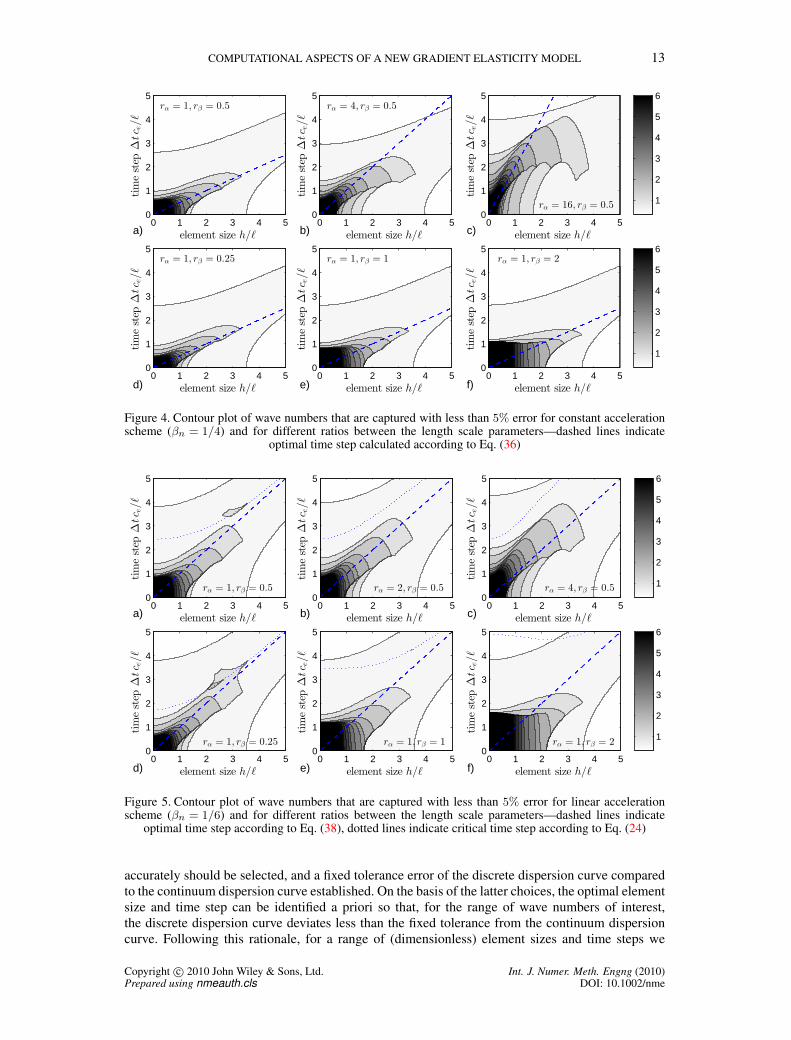
Figure 4. Contour plot of wave numbers that are captured with less than 5% error for constant accelerationscheme (βn = 1/4) and for different ratios between the length scale parameters—dashed lines indicate

optimal time step calculated according to Eq. (36)

element size h/ℓ

timestep

∆tc e/ℓ

0 1 2 3 4 50

1

2

3

4

5

element size h/ℓ

timestep

∆tc e/ℓ

0 1 2 3 4 50

1

2

3

4

5

element size h/ℓ

timestep

∆tc e/ℓ

0 1 2 3 4 50

1

2

3

4

5

1

2

3

4

5

6

element size h/ℓ

timestep

∆tc e/ℓ

0 1 2 3 4 50

1

2

3

4

5

element size h/ℓ

timestep

∆tc e/ℓ

0 1 2 3 4 50

1

2

3

4

5

element size h/ℓ

timestep

∆tc e/ℓ

0 1 2 3 4 50

1

2

3

4

5

1

2

3

4

5

6

a) b) c)

d) e) f)

rα = 1, rβ = 0.25 rα = 1, rβ = 1 rα = 1, rβ = 2

rα = 1, rβ = 0.5 rα = 2, rβ = 0.5 rα = 4, rβ = 0.5

Figure 5. Contour plot of wave numbers that are captured with less than 5% error for linear accelerationscheme (βn = 1/6) and for different ratios between the length scale parameters—dashed lines indicate

optimal time step according to Eq. (38), dotted lines indicate critical time step according to Eq. (24)

accurately should be selected, and a fixed tolerance error of the discrete dispersion curve compared

to the continuum dispersion curve established. On the basis of the latter choices, the optimal element

size and time step can be identified a priori so that, for the range of wave numbers of interest,

the discrete dispersion curve deviates less than the fixed tolerance from the continuum dispersion

curve. Following this rationale, for a range of (dimensionless) element sizes and time steps we



have computed the first (dimensionless) wave number for which the relative error of the discrete

dispersion curve as compared to the continuum dispersion curve is no more that 5%. In Figs. 4 and

5 we report the contour plot of the computed wave numbers for the constant acceleration scheme and

for the linear acceleration scheme, respectively. These graphs serve to indicate which wave numbers

are captured accurately (within the 5% tolerance) with a given set of element size and time step and

for a given set of length scale parameters. For example, from Fig. 4 b) it is noted that for rα = 4 and

rβ = 0.5 if a unitary element size and a unitary time step are adopted as discretisation parameters,

the wave numbers that are captured accurately are approximately kℓ ≈ 4 (cf. with Fig. 3 a)). This

means that if wave numbers larger than kℓ = 4 are to be simulated accurately, a more refined discrete

model should be adopted by reducing the element size and the time step accordingly. Moreover, it

can be seen that the element size and the time step should be selected proportionally. For example,

focusing the attention on Fig. 4 a), if the spatial discretisation is such that h/ℓ = 2, the best time

step that should be selected is approximately ∆ce/ℓ ≈ 1 so that wave numbers up to kℓ ≈ 2 are

captured accurately. Refining the time step further for fixed element size h/ℓ = 2 would lead to

reduce the range of wave numbers that are described accurately, and thus would worsen, instead of

improving as one would normally expect, the numerical prediction. The same result is obtained if,

vice versa, for a fixed time step the element size were refined beyond a certain value. Therefore, the

two discretisation parameters should be balanced according to an optimal ratio that depends on the

length scale parameters. By inspection of Fig. 4 a), b), c) where for a fixed rβ we vary the rα ratio, it

can be seen that a reasonable choice of the time step for the constant acceleration scheme is (cf. [9])

∆t ≈h√rα

2ce. (36)

The relation described in Eq. (36) is reported as a dashed line in the contour plots of Fig. 4. On

the other hand, the effect of the β-length scale is described in Fig. 4 d), e), f) where for a fixed rαwe vary the rβ ratio. The rβ ratio widens the range of element sizes and time steps for which a

given accuracy is achieved, rather than modifying the slope of the optimal ratio between the two

discretisation parameters. As already noted when discussing the results of Fig. 3 b), this implies

that for fixed discretisation parameters a higher accuracy is achieved for increasing values of the rβratio or, equivalently, that for large β values the requirements on the discretisation can be made less

stringent to attain a certain accuracy of the numerical solution.

Similar considerations can be made for the linear acceleration scheme, whose relevant results are

reported in Fig. 5. As in the previous case, the optimal time step should be selected proportionally

to the element size so that spatial and time discretisation are balanced. However, since the linear

acceleration scheme is only conditionally stable, the chosen time step must be smaller than the

critical time step given by Eq. (24). By looking at the profiles of the critical time step depicted in

Fig. 1 a), it seems reasonable to compute an upper bound value for the time step according to the

asymptotic slope of the ∆tcrit curves that, for the linear acceleration scheme, is given by

m = limh→∞

∂∆tcrit

∂h=

1

ce(37)

from which the optimal value for the time step is

∆t = mh =h

ce. (38)

As can be seen from Fig. 5, the upper bound value given by Eq. (38) (straight line reported in dashed)

never exceeds or intersects the critical time step curve (24) (reported in dotted line). Therefore, the

recommendation on the time step given by Eq. (38) leads to an effective combination between

accuracy and stability: it preserves stability for the all the possible values of the element size h/ℓ,but at the same time it yields much more accurate results than the critical time step (24) for small

values of the element size as illustrated in Fig. 5.



7. NUMERICAL EXAMPLES

In this Section, the guidelines discussed above are verified numerically. Using the finite element

implementation introduced in Section 2, wave propagation is examined in a one-dimensional bar

as well as in a two-dimensional body. Different numerical parameters are explored to cover a

broad range of examples, including discretisation parameters and material length scale coefficients.

For simplicity, a uniform element size h and a uniform time step ∆t are adopted throughout

as discretisation parameters. Moreover, a unitary γ coefficient is assumed for all the numerical

examples, so that the rα and rβ ratios coincide with the actual values of the α and β length scale

coefficients.

7.1. One-dimensional bar

As a first example, dispersive wave propagation in a simple one-dimensional bar is simulated. With

reference to the test set-up shown in Fig. 6, we consider a bar having length L = 100m and cross-

sectional area A = 1m2. The bar is fixed at the right hand end and subjected to a compressive

unit-pulse at its left hand end, that is, a force expressed by F = F0 δ(t), with δ(t) the Dirac delta

and F0 = 1N the unit-pulse applied at t = 0. The material parameters of the bar are the Young’s

modulus E = 1N/m2, the mass density ρ = 1 kg/m3 and the internal length scale ℓ = 1m.

LF

Figure 6. One-dimensional dynamic bar problem: geometry, loading and boundary conditions

In Fig. 7 a series of finite element meshes combined with proportionally scaled time steps

are used to investigate the convergence of the numerical solution upon refinement. The assumed

material length scale ratios are rα = 4 and rβ = 0.5. Two time integration algorithms have been

employed, namely the implicit Newmark constant acceleration scheme and the explicit 4,5-Runge-

Kutta algorithm. A reference solution for the bar problem is computed using a finite element mesh

of 2000 elements and the Newmark constant acceleration scheme with ∆t = 0.05 s. When refining

the element size, the corresponding time step is calculated according to Eq. (36). Due to the choice

of the length scale coefficients and material parameters, the optimal time step according to Eq. (36)

is such that h/∆t = 1m/s. From Fig. 7 it can be seen that the smaller wave numbers (i.e. the

longer wave lengths) travel faster than the lower wave numbers as predicted by the analytical

dispersion curve (11) for α > γ. This holds for both the microscopic displacements um and the

macroscopic displacements uM , although in general the latter profile is smoother than the former

owing to Eq. (2b) that relates the two displacement fields. Upon refinement both the displacements

converge rapidly towards the reference solution for both the time integration methods. The two time

integration methods create opposite errors with respect to the reference solution due to the fact that

the implicit (explicit) schemes generally provide a lower (upper) bound value for the frequency

of the exact solution. By comparing the numerical solutions of the two integration methods, the

implicit method seems to be more accurate on the higher frequencies (around the tail of the wave)

than the Runge-Kutta method, whereas the explicit method tends to behave in the opposite way and

captures the front of the wave more accurately for equal time step.

Convergence upon refinement towards the reference solution is achieved only if element size

and time step are refined proportionally. It is counterproductive to decrease either element size

or time step without decreasing the other simultaneously. By keeping the same material length

scale parameters as above, we consider a coarse solution obtained with h = 2m for the spatial

discretisation and the constant acceleration scheme with ∆t = 2s for the time discretisation. We

investigate the effect of either sole element size refinement or sole time step refinement. In Fig. 8

we report the profiles of the macroscopic displacements uM when the element size is refined by a

factor 4 and 16 for fixed time step (Fig. 8 a)), and when the time step is refined by a factor 4 and 16



0 20 40 60 80 1000

0.2

0.4

0.6

0.8

1

1.2

1.4

x [mm]

um[m

m]

h = 4,∆t = 4h = 2,∆t = 2h = 1,∆t = 1reference

0 20 40 60 80 1000

0.2

0.4

0.6

0.8

1

1.2

1.4

x [mm]

uM

[mm]


0 20 40 60 80 1000

0.2

0.4

0.6

0.8

1

1.2

1.4

x [mm]

um[m

m]


0 20 40 60 80 1000

0.2

0.4

0.6

0.8

1

1.2

1.4

x [mm]

uM

[mm]


a) b)

c) d)

Figure 7. Dispersive wave propagation along the bar of Fig. 6 at t = 80s—convergence upon proportional

element size/time step of the micro-displacements um and macro-displacements uM : a), b) implicitNewmark constant acceleration scheme; c), d) explicit Runge-Kutta (4,5) algorithm

0 20 40 60 80 1000

0.2

0.4

0.6

0.8

1

1.2

1.4

x [mm]

uM

[mm]

∆t = 2∆t = 0.5∆t = 0.125reference

0 20 40 60 80 1000

0.2

0.4

0.6

0.8

1

1.2

1.4

x [mm]

uM

[mm]

h = 2h = 0.5h = 0.125reference

a) b)

∆t = 2 h = 2

Figure 8. Wave propagation along the bar depicted in Fig. 6 at t = 80s: a) effect of sole element sizerefinement for fixed time step; b) effect of sole time step refinement for fixed element size

for fixed element size (Fig. 8 b)). In either case the numerical solution converges towards a profile

that is different from the reference solution, which indicates that such refinement strategies are not

effective.



0 20 40 60 80 1000

0.2

0.4

0.6

0.8

1

1.2

1.4

x [mm]

um[m

m]

∆t = 0.5∆t = 1.98∆t = 2.0reference

0 20 40 60 80 1000

0.2

0.4

0.6

0.8

1

1.2

1.4

x [mm]

uM

[mm]

∆t = 0.5∆t = 1.98∆t = 2.0reference

a) b)

h = 0.5 h = 0.5

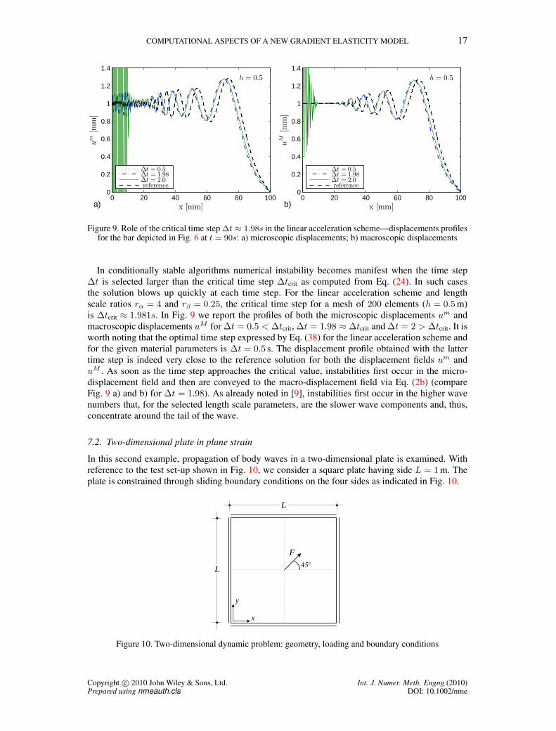
Figure 9. Role of the critical time step ∆t ≈ 1.98s in the linear acceleration scheme—displacements profilesfor the bar depicted in Fig. 6 at t = 90s: a) microscopic displacements; b) macroscopic displacements

In conditionally stable algorithms numerical instability becomes manifest when the time step

∆t is selected larger than the critical time step ∆tcrit as computed from Eq. (24). In such cases

the solution blows up quickly at each time step. For the linear acceleration scheme and length

scale ratios rα = 4 and rβ = 0.25, the critical time step for a mesh of 200 elements (h = 0.5m)

is ∆tcrit ≈ 1.981s. In Fig. 9 we report the profiles of both the microscopic displacements um and

macroscopic displacements uM for ∆t = 0.5 < ∆tcrit, ∆t = 1.98 ≈ ∆tcrit and ∆t = 2 > ∆tcrit. It is

worth noting that the optimal time step expressed by Eq. (38) for the linear acceleration scheme and

for the given material parameters is ∆t = 0.5 s. The displacement profile obtained with the latter

time step is indeed very close to the reference solution for both the displacement fields um and

uM . As soon as the time step approaches the critical value, instabilities first occur in the micro-

displacement field and then are conveyed to the macro-displacement field via Eq. (2b) (compare

Fig. 9 a) and b) for ∆t = 1.98). As already noted in [9], instabilities first occur in the higher wave

numbers that, for the selected length scale parameters, are the slower wave components and, thus,

concentrate around the tail of the wave.

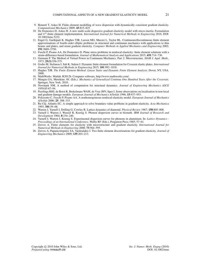
7.2. Two-dimensional plate in plane strain

In this second example, propagation of body waves in a two-dimensional plate is examined. With

reference to the test set-up shown in Fig. 10, we consider a square plate having side L = 1m. The

plate is constrained through sliding boundary conditions on the four sides as indicated in Fig. 10.

L

F

L 45

x

y

Figure 10. Two-dimensional dynamic problem: geometry, loading and boundary conditions



−0.05 0 0.05

−0.05 0 0.05

−0.1 −0.05 0 0.05 0.1

−0.02 −0.01 0 0.01 0.02

−0.02 −0.01 0 0.01 0.02

−0.04 −0.02 0 0.02 0.04

a) b) c)

d) e) f)

ε cxx ε c

yy γcxy

εMxx εMyy γMxy

Figure 11. Two-dimensional dynamic problem sketched in Fig. (10)—contour plot, reported onto thedeformed shape of the plate, of strain components at t = 0.05s for mesh 32× 32: a), b), c) results of classical

elasticity; d), e) f) results of gradient elasticity

Propagation of body waves is triggered by a point load F applied at the centre of the specimen

and forming a 45 angle to the x axis. The force is expressed as F = F0 U(t), where F0 =√2N is

a constant stepforce at time t = 0 and the function U(t) represents the Heaviside unit-step function.

The plate is assumed to be in a plane strain configuration with the following material parameters:

Young’s modulus E = 100N/m2, Poisson’s ratio ν = 0.25, mass density ρ = 1 kg/m3 and internal

length scale ℓ = 0.05m. The values of the length scale ratios for this example are rα = 4 and rβ = 2.

Uniform meshes of four-noded bilinear quadrilateral elements are used. The Newmark constant

acceleration scheme is employed for the time integration. As suggested in [9], the time step ∆tis computed through a heuristic generalisation of Eq. (36) to two dimensions, in which the one-

dimensional bar velocity of classical elasticity ce is replaced by the compressive wave velocity cp(cf. Section 3).

Singularities are expected in classical elasticity at the position where the point load is applied. We

investigate the removal of singularities of the proposed formulation of gradient elasticity as well as

the validity of the aforementioned recommendations for selecting discretisation parameters for two-

dimensional cases. The results of the gradient elasticity model are reported in Fig. 11 and compared

to the classical elasticity solution for a mesh consisting of 32× 32 square elements. Contour plots

of the macroscopic strain components are reported onto the deformed shape of the plate at time

t = 0.05s, which is approximately equal to the time for the wave front to propagate from the centre

of the specimen to the edges of the domain. The same scaling factor is used to magnify the deformed

shapes of classical and gradient elasticity. As can be seen, a smooth profile of the displacements as



0 0.2 0.4 0.6 0.8 10

0.004

0.008

0.012

0.016

x [m]

uc x[m

]

8 × 816 × 1632 × 3264 × 64

0 0.2 0.4 0.6 0.8 10

0.005

0.01

0.015

0.02

x [m]

um x[m

]

8 × 816 × 1632 × 3264 × 64

0 0.2 0.4 0.6 0.8 10

0.002

0.004

0.006

0.008

x [m]

uM x

[m]

8 × 816 × 1632 × 3264 × 64

0 0.2 0.4 0.6 0.8 1−0.005

0

0.005

0.01

0.015

0.02

x [m]

uc y[m

]

8 × 816 × 1632 × 3264 × 64

0 0.2 0.4 0.6 0.8 10

0.005

0.01

0.015

0.02

x [m]

um y[m

]

8 × 816 × 1632 × 3264 × 64

0 0.2 0.4 0.6 0.8 10

0.002

0.004

0.006

0.008

x [m]

uM y

[m]

8 × 816 × 1632 × 3264 × 64

a) b)

c) d)

e) f)

Figure 12. Two-dimensional dynamic problem sketched in Fig. (10)—profile of the displacements along thesection y = L/2 at t = 0.05s: a), b) classical elasticity displacements; c), d) microscopic displacements; e),

f) macroscopic displacements

well as of the strain components is achieved by the gradient elasticity model, whereas the classical

elasticity results exhibit a singularity at the centre of the specimen.

To assess the removal of singularities more in-depth, we perform a mesh refinement study by

using 8× 8, 16× 16, 32× 32 and 64× 64 square elements of size h. The displacement profiles

along the section y = L/2 are reported in Fig. 12. It can be seen that singularities are detected

not only in classical elasticity, but also in the microscopic displacements and strains of the

gradient elasticity where unbounded peaks are found at the point x = L/2. Conversely, singularities

disappear in the macroscopic displacement field (and, consequently, in the macroscopic strains as

shown in Fig. 11). This aspect has already been clarified in [4, 8]: the differential equation that

relate the macroscopic displacements to the microscopic displacements (uMi − γℓ2uM

i,nn = umi ) can

be rewritten as an equivalent integral nonlocal relation [19] in which the uMi variables are interpreted

as the weighted (nonlocal) average of the umi variables in a certain finite neighbourhood. Therefore,



singularities in the microscopic displacements are eliminated at the macroscale level of observation

when umi are mapped into the volume-averaged variables uM

i . By inspection of Fig. 12 e), f), it is

observed that the macroscopic displacements uM are free of singularities and converge towards a

unique solution upon mesh refinement. Furthermore, the displacement profiles pertaining to the four

analysed meshes are actually very close to each other, which indicates, at least from a qualitative

point of view, that the guidelines established for the 1D case can be applied to 2D examples.

8. CONCLUDING REMARKS

In this contribution, we have discussed a few computational aspects of a recently developed gradient

elasticity model for dynamics. The proposed model incorporates three gradient terms, namely a

strain gradient and two micro-inertia contributions, accompanied by three length scale parameters.

The relative magnitudes between the three length scales are adjusted by three coefficients (α, β,

γ) introduced in the formulation. Finite element implementation of this model has already been

discussed in [10]. The computational aspects examined in this paper concern spatial and time

discretisation details.

Dispersion analysis with reference to two-dimensional body waves has been performed to find

analytical dispersion curves for compressive and shear waves. It has been found that these two

dispersion curves have the same shape, whereby the strain gradient term accelerates while the

micro-inertia terms decelerate the higher wave numbers compared to the lower wave numbers.

The discretised equations of the higher-order continuum are then analysed more in-depth. Since

a diagonally lumped mass matrix would cancel the higher-order effects, there would be no

computational advantages in using an explicit time integration, whereas implicit methods (e.g. the

Newmark scheme) are preferable because of accuracy and stability reasons. Therefore, we have

investigated some computational aspects regarding the discretised equations in which the Newmark

family is employed for the time integration. Firstly, stability aspects are analysed for conditionally

stable variants of the Newmark family. It has been illustrated how the critical time step depends

on the three length scale parameters of the model. Secondly, accuracy aspects are investigated

by comparing the analytical dispersion curve of the higher-order continuum with that of the

discretised medium. Once the length scale parameters for a given physical problem are calibrated

and once the significant range of wave numbers that need to be simulated accurately is identified,

the discretisation parameters can be selected a priori so that the discrete dispersion curve differs

less than a fixed tolerance error from the continuum dispersion curve. In light of this, some

guidelines have been established to select optimal values for the discretisation parameters that

balance computational efficiency and numerical accuracy. The validity of these guidelines has been

verified numerically by exploring the wave propagation in a few simple examples.

REFERENCES

1. Aifantis EC. On the role of gradients in localization of deformation and fracture. International Journal ofEngineering Science 1992; 30:1279–1299.

2. Altan B, Aifantis EC. On some aspects in the special theory of gradient elasticity. Journal of the MechanicalBehavior of Materials 1997; 8: 231-282.

3. Askes H, Aifantis EC. Gradient elasticity theories in statics and dynamics - a unification of approaches.International Journal of Fracture 2006; 139:297-304.

4. Askes H, Aifantis EC. Gradient elasticity in statics and dynamics: an overview of formulations, length scaleidentification procedures, finite element implementations and new results. International Journal of Solids andStructures 2011; 48:1962-1990.

5. Askes H, Bennett T, Aifantis EC. A new formulation and C 0-implementation of dynamically consistent gradientelasticity. International Journal for Numerical Methods in Engineering 2007; 72:111-126.

6. Askes H, Metrikine AV. One-dimensional dynamically consistent gradient elasticity models derived from a discretemicrostructure. Part 2: Static and dynamic response. European Journal of Mechanics – A/Solids 2002; 21:573–588.

7. Bazant ZP, Jirasek M. Nonlocal integral formulations of plasticity and damage: survey of progress. Journal ofEngineering Mechanics 2002; 11:1119–1149.

8. Bennett T, Gitman I, Askes H. Elasticity theories with higher-order gradients of inertia and stiffness for themodelling of wave dispersion in laminates. International Journal of Fracture 2007; 148:185–193.



9. Bennett T, Askes H. Finite element modelling of wave dispersion with dynamically consistent gradient elasticity.Computational Mechanics 2009; 43:815–825.

10. De Domenico D, Askes H. A new multi-scale dispersive gradient elasticity model with micro-inertia: Formulationand C 0-finite element implementation. International Journal for Numerical Methods in Engineering 2016, DOI:10.1002/nme.5222.

11. Engel G, Garikipati K, Hughes TJR, Larson MG, Mazzei L, Taylor RL. Continuous/discontinuous finite elementapproximations of fourth-order elliptic problems in structural and continuum mechanics with applications to thinbeams and plates, and strain gradient elasticity. Computer Methods in Applied Mechanics and Engineering 2002;191:3669–3750.

12. Fuschi P, Pisano AA, De Domenico D. Plane stress problems in nonlocal elasticity: finite element solutions with astrain-difference-based formulation. Journal of Mathematical Analysis and Applications 2015; 431:714–736.

13. Germain P. The Method of Virtual Power in Continuum Mechanics. Part 2: Microstructure. SIAM J. Appl. Math.,1973; 25(3):556-575.

14. Godio M, Stefanou I, Sab K, Sulem J. Dynamic finite element formulation for Cosserat elastic plates. InternationalJournal for Numerical Methods in Engineering 2015; 101:992–1018.

15. Hughes TJR. The Finite Element Method: Linear Static and Dynamic Finite Element Analysis. Dover, NY, USA.2000.

16. MathWorks. Matlab. R2012b. Computer software, http://www.mathworks.com/.17. Maugin GA, Metrikine AV. (Eds.). Mechanics of Generalized Continua One Hundred Years After the Cosserats.

Springer, New York. 2010.18. Newmark NM. A method of computation for structural dynamics. Journal of Engineering Mechanics ASCE

1959;85:67–94.19. Peerlings RHJ, de Borst R, Brekelmans WAM, de Vree JHV, Spee I. Some observations on localisation in non-local

and gradient damage models. European Journal of Mechanics A/Solids 1996; 15:937–953.20. Polizzotto C, Fuschi P, Pisano AA. A nonhomogeneous nonlocal elasticity model. European Journal of Mechanics

A/Solids 2006; 25: 308–333.21. Ru CQ, Aifantis EC. A simple approach to solve boundary-value problems in gradient elasticity. Acta Mechanica

1993; 101:59–68.22. Warren J, Yarnell J, Dolling G, Cowley R. Lattice dynamics of diamond. Physical Review 1967; 158:805–808.23. Yarnell J, Warren J, Wenzel R, Koenig S. Phonon dispersion curves in bismuth. IBM Journal of Research and

Development 1964; 8:234–240.24. Yarnell J, Warren J, Koenig S. Experimental dispersion curves for phonons in aluminium. In: Lattice Dynamics -

Proceedings of an International Conference, Wallis RF (Eds.), Pergamon Press 1965; 57–61.25. Zervos A. Finite elements for elasticity with microstructure and gradient elasticity. International Journal for

Numerical Methods in Engineering 2008; 73:564–595.26. Zervos A, Papanicolopulos SA, Vardoulakis I. Two finite element discretizations for gradient elasticity. Journal of

Engineering Mechanics 2009; 135:203–213.


computational aspects of a new multi-scale...

Documents