Computational and Theoretical Chemistry 1006 (2013) 92–99

Contents lists available at SciVerse ScienceDirect

Computational and Theoretical Chemistry

journal homepage: www.elsevier .com/locate /comptc

Pauli potential and Pauli charge from experimental electron density

Vladimir G. Tsirelson a,⇑, Adam I. Stash a,b, Valentin V. Karasiev c, Shubin Liu d,⇑a Quantum Chemistry Department, Mendeleev University of Chemical Technology, Moscow 125047, Russiab Karpov Institute of Physical Chemistry, Moscow 105064, Russiac Quantum Theory Project, Departments of Physics and of Chemistry, University of Florida, Gainesville, FL 32611, United Statesd Research Computing Center, University of North Carolina, Chapel Hill, NC 27599-3420, United States

a r t i c l e i n f o

Article history:Received 11 July 2012Received in revised form 18 November 2012Accepted 20 November 2012Available online 29 November 2012

Keywords:Chemical bondDensity functional theoryElectron density

2210-271X/$ - see front matter � 2012 Elsevier B.V.http://dx.doi.org/10.1016/j.comptc.2012.11.015

⇑ Corresponding authors. Tel.: +7 499 978 958(V. Tirelson), tel.: +1 919 962 4032; fax: +1 919 9

E-mail addresses: vtsirelson@yandex.ru (V.G. Tsire(S. Liu).

a b s t r a c t

In this work, based on the experimental electron density, we present the approximate spatial distribu-tions of the Pauli potential, one of the key quantities in the orbital-free density functional, for three crys-talline systems: diamond, cubic boron nitride, and magnesium diboride. Our aim is to reveal a linkbetween the Pauli potential and the orbital-free picture of chemical bond. We also expand the theoreticalframework by developing the concept of the Pauli charge density. We find that both these quantitiesreproduce the electronic shell structure in the atomic core regions, while in the bonding region theyreveal the different features for different bonding types, thereby distinguishing between ionic and cova-lent bond and also identifying the distinction between polar and nonpolar covalent bonds. Therefore, thePauli potential and its associated charge density can be used as the orbital-free descriptors of chemicalbond in the crystalline systems.

� 2012 Elsevier B.V. All rights reserved.

1. Introduction

Density functional theory (DFT) has become one of the mostpowerful tools in computing the electronic structure of moleculesand solids [1,2]. It is both theoretically rigorous and computation-ally efficient. From another side, recent progress in the X-ray dif-fraction instrumentation [3,4] provides an opportunity for furtherdevelopment of the experimental data treatment methods to be-come a reliable tool in the detailed study of the physical and chem-ical properties of solids, which are defined by the electron density.Naturally, these methods are based on density functional theoryand usually include quantum-topological analysis of electron den-sity from the bonding point of view [5,6]. However, the most pop-ular implementation of DFT makes use of the Kohn–Sham scheme[7], in which single-particle orbitals are introduced and the non-interacting kinetic energy is treated exactly instead of usingapproximate density functionals [8]. The computational complex-ity of the Kohn–Sham scheme goes at least as N3 in a plane wavebasis set or N4 in a localized one, where N is the total number ofelectrons or basis functions. This relatively high computationalcost restricts the extent to which the Kohn–Sham method can beapplied to the simulation of large systems of biological and mate-rial science relevance. In the recent literature of DFT developments,

All rights reserved.

4; fax: +7 495 609 296462 0417 (S. Liu).lson), shubin@email.unc.edu

we have witnessed a renewed surge of efforts to use the densityand its derivatives only in the simulation of electronic propertiesof molecules and crystals. This latter approach is often called orbi-tal-free DFT (OF-DFT), see [9–12] for reviews. The attractiveness ofthe OF-DFT approach lies in the fact that regardless of the systemsize, the problem size scales at worst with the volume. However,the difficulty of developing physically valid approximations forthe non-interacting kinetic energy density functional has limitedthe development of effective OF-DFT methods [13–24] severely.The use of orbital-free methods is almost inescapable, however,for the case in which only the electron density reconstructed fromX-ray diffraction data is used as the input for analysis of physicaland chemical properties. From the viewpoint of developing newapproximate orbital-free functionals, the data retrieved fromexperiments may serve as a reference exactly in the same way asdata obtained from the high-level theory.

In the OF-DFT approach, instead of a self-consistent problem fora set of KS orbitals, one obtains a single Euler equation by minimiz-ing the total energy density functional E[q] subject to the con-straint that the total electron density q(r) is normalized to thetotal number of electrons. The Euler equation has the followingSchrödinger-like form [25–27],

f�1=2r2 þ vhðrÞ þ veff ðrÞgq1=2ðrÞ ¼ lq1=2ðrÞ; ð1Þ

where l is the chemical potential, vh(r) is the Pauli potential, andveff(r) is the effective potential. The last quantity is in fact the stan-dard Kohn–Sham potential. It can be decomposed further into thefollowing contributions,

V.G. Tsirelson et al. / Computational and Theoretical Chemistry 1006 (2013) 92–99 93

veff ðrÞ ¼ vesðrÞ þ vxcðrÞ: ð2Þ

The electrostatic potential, ves(r), is the sum of the external po-tential, vext(r), and the classical inter-electron Columbic repulsionpotential, vJ(r),

vesðrÞ ¼ vextðrÞ þ v JðrÞ ¼ �X

a

Za

jr� RajþZ

qðr0Þjr� r0j dr0: ð3Þ

The exchange–correlation potential, vxc(r), is defined as thefunctional derivative of the exchange–correlation energy func-tional Exc[q],

vxcðrÞ ¼dExc½q�

dq: ð4Þ

The term vh(r) in Eq. (1), the Pauli potential [27, 28], stems fromthe effect of the many-electron wave function anti-symmetryrequirement in the kinetic energy [29–31].

Given a system and exchange–correlation functional approxi-mation, the Pauli potential can be obtained readily via theKohn–Sham orbitals and eigenvalues {ui,ei} as [29]

vhðrÞ ¼XN=2

i¼1

½rðuiq�1=2Þ� � rðuiq

�1=2Þ þ ðeN=2 � eiÞ2u�i uiq�1�; ð5Þ

for the case of N/2 doubly occupied orbitals. The non-negativity ofvh(r) is one of the exact properties of the Pauli potential which fol-lows from Eq. (5). At the same time, to the best of our knowledge, nonumerical data has been available in the literature for the Paulipotential obtained from the electron density without the use ofone-electron orbitals, except for a few atomic and molecular cases[12,22,32]. In this work, we report the first examples of the Paulipotential for a few crystalline systems, namely diamond, cubic bor-on nitride, and magnesium diboride, approximately reconstructedfrom experimental (X-ray and synchrotron) electron density mea-sured by accurate diffraction methods. We are also interested inexploring how the chemical bonding features derived from experi-ment manifest themselves in the Pauli potential in the crystals withdifferent bonding types. Similar studies, for the case of theoreticalKohn–Sham densities, have already been reported for the compo-nents of the Kohn–Sham local potentials in atoms [33] and diatomicmolecules [34]. In addition, the corresponding charge densities de-fined through the Poisson equation from the Pauli potential are alsopresented in this work.

2. Theoretical framework

Conventionally, the total energy density functional E[q] can bedecomposed into the non-interacting kinetic energy Ts[q], the elec-trostatic energy Ees[q], and the exchange–correlation energy Exc[q],

E½q� ¼ Ts½q� þ Ees½q� þ Exc½q� ð6Þ

where Ees[q] is the sum of the electron-nuclear attraction Een[q], nu-clear–nuclear repulsion Enn, and the classical Columbic repulsionJ[q],

Ees½q� ¼ Een½q� þ Enn þ J½q�: ð7Þ

The exchange–correlation energy, Exc[q], includes the kineticcounterpart of so-called the dynamic electron correlation[35–37]. The foregoing energy decomposition can be re-arrangedto separate the Weizsäcker kinetic energy [38]

TW ½q� ¼18

Z jrqðrÞj2

qðrÞ dr ¼ 12

Zjr½q1=2ðrÞ�j2dr ð8Þ

giving

E½q� ¼ TW ½q� þ Th½q� þ Ees½q� þ Exc½q�; ð9Þ

with the Pauli energy Th[q], defined as

Th½q� B Ts½q� � TW ½q�; ð10Þ

where Ts[q] is the Kohn–Sham non-interacting kinetic energyfunctional.

The Pauli potential is defined as the functional derivative of thePauli energy, Th[q], with respect to the electron density:

vhðrÞ ¼dTh½q�

dq¼ dTs½q�

dq� dTW ½q�

dq: ð11Þ

Here the term dTW ½q�dq ¼ vW ðrÞ is the von Weizsäcker potential

(which was recently treated as the steric electronic potential [39]):

vW ðrÞ ¼18jrqðrÞj2

q2ðrÞ �14r2qðrÞqðrÞ : ð12Þ

Two approaches are available to express the Pauli potential, Eq.(11), explicitly in terms of the electron density and its gradients.One can use an approximate form of either the kinetic energy den-sity functional or the exchange–correlation energy density func-tional. To obtain the explicit expression for the functionalderivative of the non-interacting kinetic energy functional, dTs ½q�

dq ,we can approximate the non-interacting kinetic energy density,ts(r), in Ts[q] =

Rts(r)dr, within the gradient expansion or conjoint

approximations [12]. For example, the Kirzhnits [40] second-ordergradient approximation yields

tsðrÞ ¼ cTFqðrÞ5=3 þ 172jrðrÞj2qðrÞ þ

16r2qðrÞ; cTF ¼

310ð3p2Þ2=3 ð13Þ

leading to

dTs½q�dq

¼ 53

cTFqðrÞ2=3 þ 172

jrqðrÞj2

q2ðrÞ � 2r2qðrÞqðrÞ

( )

¼ 53

cTFqðrÞ2=3 þ 19

vWðrÞ: ð14Þ

As a result, the approximate Pauli potential can be expressed inthe form

vhðrÞ ¼53

cTFqðrÞ2=3 � 89

vWðrÞ: ð15Þ

Note that this approach is close to that already exploited byKing and Handy [41].

Another way to construct the Pauli potential is to use the EulerEq. (1) which can be presented in the standard form [42]

dTs½q�dq

¼ l� veff ðrÞ ð16Þ

For a given system, l = const. The effective potential veff(r) is de-fined up to an arbitrary constant, therefore it is convenient to setl = 0 throughout this work [41]. It is assumed that for finite atomicsystems veff(r) ? 0 with r ?1 and vh(r) ? 0 with r ?1 [29]. Alsothe Pauli potential will vanish in the special case of one electron ortwo electron (singlet) systems.

Taking into account of Eq. (11), we arrive at the followingexpression for the Pauli potential:

vhðrÞ ¼ �vesðrÞ � vxcðrÞ � vWðrÞ: ð17Þ

This way of computing the Pauli potential, in contrast to Eq. (15),does not involve the use of an approximate kinetic energy func-tional, but uses an approximate form for the exchange–correlationterm. Decomposing the exchange–correlation potential vxc(r) intothe exchange, vx(r), and correlation, vc(r), parts, vxc(r) = vx(r) + vc(r),we can calculate it by the known approximate exchange and corre-lation functional formulas. The simplest one is to use the local

94 V.G. Tsirelson et al. / Computational and Theoretical Chemistry 1006 (2013) 92–99

density approximation (LDA) to obtain vx(r) and vc(r) potentials. Inthis work, we employed the von Barth–Hedin exchange and correla-tion potentials [43].

Eq. (5) can also be used to evaluate the Pauli potential in casethat both the density and KS orbitals are given. In that case, ifthe same approximation is used for the exchange–correlation term,Eq. (5) will produce exactly the same result as Eq. (17) (see Ref.[29] for details).

The Pauli charge density, qh(r), may be defined for potential vh

by means of the Poisson equation [44–46]

r2vhðrÞ ¼ �4pqhðrÞ: ð18Þ

In contrast to the potential vh, the associated Pauli charge den-sity qh(r) can be both positive and negative. It also does not dependon an arbitrary constant, such as the case for the constant l in Eq.(16). It is worth noting that the function �qh(r) =r2vh(r) ‘‘works’’in the same manner as Laplacian of the electron density. Therefore,this function may be helpful in the topological analysis of the Paulipotential from the bonding viewpoint.

3. Computational details

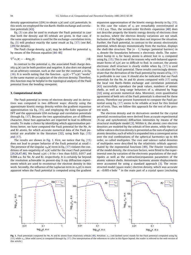
The Pauli potential in terms of electron density and its deriva-tives was computed in two different ways: directly using theapproximate kinetic energy density within the gradient expansionapproximation via Eq. (15), and employing the Euler equation ofDFT and the approximate LDA exchange and correlation potentialsthrough Eq. (17). Because the two approximations are of differentcharacter, these two approaches are expected to lead to differentresults. To make a choice by identifying which approximation per-forms better, we have computed the Pauli potential for the Ne, Arand Kr atoms, for which accurate numerical data of the Pauli po-tential are available in the literature [32], using both Eqs. (15)and (17).

The results are shown in Fig. 1. First, we notice that Eq. (15)does not lead to proper behavior of the Pauli potential at small r.The presence of the singular vW(r) term in Eq. (17) violates the con-ditions of non-negativity of vh(r) valid for the exact Pauli potential[29,26,47,48]. We found vh(r) 6 0 for r less than 0.033, 0.017 and0.008 a.u. for Ne, Ar and Kr, respectively. It is certainly far beyondthe resolution achievable in present-day X-ray diffraction experi-ments which are used to reconstruct the electron density in thiswork. Secondly, the influence of the Laplacian term in vW(r) is moreapparent when the Pauli potential is computed using the gradient

Fig. 1. Pauli potentials computed for Ne, Ar and Kr atoms from relativistic orbitals [49].(15), while vh,2 (blue solid curve) is computed through Eq. (17). (For interpretation of thethis article.)

expansion approximation of the kinetic energy density in Eq. (15).In this case the values of vh are remarkably overestimated atr < 0.1 a.u. Thus, the second-order Kirzhnits expansion [40] doesnot describe properly the kinetic energy density of electrons closeto nucleus, where the electron density variations are not small.Inclusion of the higher-order terms does not improve the situation.Further, the Pauli potential, in contrast to the atomic electrostaticpotential, which decays monotonically from the nucleus, displaysthe shell-like structure. The (n � 1) humps (potential barriers) invh denote the boundaries between n electronic shells. The outer-most hump in vh for heavy atoms is almost lost in vh computedusing Eq. (15). This is one of the reasons why well-behaved approx-imate forms of tS(r) are so difficult to find. In contrast, the atomicelectronic shell structure is clearly visible when Eq. (17) is usedto calculate the Pauli potential. These results convincingly demon-strate that the derivation of the Pauli potential by means of Eq. (17)is preferable in our case. It should also be indicated that our Paulipotentials for the Ne, Ar and Kr atoms computed with (17) usingthe local von Barth–Hedin exchange and correlation potentials[43] successfully reproduce the peak values, numbers of atomicshells, as well as long range behaviors of vh obtained by Nagy[32] using accurate numerical data. Moreover, even quantitativeagreement of both sets of the Pauli potentials is observed for theseatoms. Therefore our present framework to compute the Pauli po-tential using Eq. (17) seems to be reliable at least for this limitedset of tests. Thus, we follow this approach for the rest of the pres-ent work.

The electron density and its derivatives needed for the crystalpotential reconstruction were derived from accurate experimental(X-ray and synchrotron) diffraction intensities by means of thestructural multipole model [3]. Within it, the atomic core electrondensities are modeled by the orbitals of free atoms, while the crys-talline valence electron density is presented as the sum of asphericalatomic densities, each of which is expanded into a convergent seriesover the real combinations of the spherical harmonics up to 4thorder, so called multipoles. The core and valence radial densitiesof multipoles were described by the relativistic orbitals approxi-mated by the exponential functions [49]. The Fourier transformsof the model density, the structure factors, were fitted to the exper-imental ones by variation of the electronic populations of the mul-tipoles as well as the contraction/expansion parameters of theatomic valence shells. Anisotropic harmonic atomic displacementswere accounted for using a standard approach [3]. The recon-structed model (quasi-static) electron density, which was accurateas �0.005 e bohr�3 in the main part of a crystal space (excluding

Notation: vh,1 (red dashed curve) stands for the Pauli potential computed using Eq.references to color in this figure legend, the reader is referred to the web version of

V.G. Tsirelson et al. / Computational and Theoretical Chemistry 1006 (2013) 92–99 95

the regions around the nuclei [50]) was used in the following calcu-lations. For diamond, the multipole-model parameters were derivedusing synchrotron experimental intensities [51]. The multipoleparameters for BN and MgB2 were taken from our previous works[52,53]. All the results described in this work were obtained usingthe program WinXPRO [54,55]. We also computed the deformationelectron densities for all crystals studied in this work to facilitate thetreatment of the potentials and to verify the reliability of our pres-ent computational results.

We note that the experimental ground-state electron density isobtained avoiding the variation principle and the self-consistent-field procedure. The experimental and computational electrondensities are also derived using the different basis sets. Therefore,there are subtle differences between these densities, which reach�0.005–0.010 a.u. in the interatomic space (for atoms withZ < 18), as is well-documented in the literature [3,4]. An experimen-tal electron density is derived with similar accuracy, as is indicatedabove. This accuracy is sufficient to compute some density-basedproperties of molecules and solids with good agreement with inde-pendent experimental data [3]. Note that our earlier works [56,57]confirm the feasibility of employing experimental electron densi-ties for approximation of the DFT functionals. Taking into accountthese facts, we employ the experimental electron density in thiswork.

4. Results and discussion

The Pauli potential and corresponding charge density for dia-mond, boron nitride (BN), and MgB2 crystals are presented in Figs.2–4, respectively. As shown in Fig. 2a, the Pauli potential vh(r) indiamond peaks on the nuclear positions, decays smoothly and thenforms near spherical barriers with a diameter �0.24 Å around eachnucleus. These barriers clearly denote the boundaries between Kand L electronic shells of bonded carbon atoms in diamond.Between atomic cores, the Pauli potential diminishes and formsextended near-uniform areas along the nonpolar C–C covalentbond. This reduced Pauli potential reflects the impact of the Pauliexclusion principle on the electronic kinetic energy and promoteselectron density accumulation along the C–C bond, as reflected inthe deformation electron density [3] (see Fig. 1S in Supplementarymaterial) That the Pauli potential distribution is symmetrical along

Fig. 2. The Pauli potential (a) and its associated charge density (b) for diamond in the (11densities, while the blue curves denote the negative values. Line intervals are 0.1 a.uinterpretation of the references to color in this figure legend, the reader is referred to th

the C–C bond is a manifestation of the fact that the C–C bond indiamond is nonpolar and covalent. From the vh(r) plot in Fig. 2a,we also can see that the regions of the reduced Pauli potentialare slightly compressed by the atomic cores along the C–C line.This however does not influence the near spherical shape of theelectron accumulation in the (110) plane, which is defined bythe whole set of bonding mechanisms. The potential vh(r) in thetetrahedral and octahedral crystal holes of diamond also showsthe barrier reflecting the symmetry of the atomic positions andseparating the zigzag chains of C atoms in the (110) plane.

These results show how the antisymmetry of the diamondmany-electron wave function influences the kinetic energy withinatomic cores, promotes formation of regions of reduced Pauli po-tential around the midpoint of the C–C and contributes to theshape of the tetrahedral and octahedral holes of the potential inthe crystal. Compared to the free carbon atom superposition(not shown), we do not observe significant changes in heightand position in the Pauli potential barrier that separates the Kand L electron shells of bonded carbon atoms. However, thebehaviors of the Pauli potential near the nuclei are substantiallydifferent. The key feature from the Pauli potential as comparedwith the free carbon atoms is the extended regions of reducedPauli potential between atomic cores. These regions with the sym-metry axis along the C–C bonds coincide with the regions of elec-tron density accumulation in diamond. These results indicate thatthe Pauli potential distribution along the C–C bond is a clear indi-cation and manifestation of the homonuclear nonpolar covalentbond.

The associated Pauli charge density, qh(r), Fig. 2b, also showsboth the atomic shell structure and the bonding features of bondedatoms in diamond clearly. The charge density qh(r) exhibits posi-tive peaks at the nuclear positions, and alternating regions ofdepletion and concentration with negatively-valued local maxi-mum of qh(r) at the middle of the C–C covalent bonds. This picturesignals that vh(r) is locally depleted in such region (qh(r) < 0).Simultaneously, the local concentration of the Pauli potential(qh(r) > 0) is observed in the crystal holes. Note that positive areasof qh(r) around atomic cores coincide with maxima in vh(r).

Put together, these results demonstrate that the three-dimen-sional distributions of the Pauli potential and corresponding chargedensity provide orbital-free information about both the atomic

0) plane. Here and below the red curves correspond to positive values of the charge. for Pauli potential and ±2, 4, 8 � 10n (�2 < n < 3) a.u. for charge density. (Fore web version of this article.)

Fig. 3. The Pauli potential (a) and its associated charge density (b) for boron nitride, BN, plane (110). Contour intervals are 0.1 a.u. for the Pauli potential and ±2, 4, 8 � 10n

(�2 < n < 3) a.u. for the charge density.

96 V.G. Tsirelson et al. / Computational and Theoretical Chemistry 1006 (2013) 92–99

inner shell structure and the nonpolar covalent bonding features atleast for this crystalline system.

Fig. 3 shows the results for the boron nitride crystal with thecubic sphalerite structure. The Pauli potential in BN also peaks atthe nuclear positions and displays potential barriers between Kand L electronic shells of both atoms. However, in contrast todiamond, the asymmetrical nature of the surroundings causesthe shape of these barriers to be non-spherical and the barrier istwice as high for the N atom as compared with B atom. The dis-tance from the barrier maximum to the boron position is 0.33 Åand that to the nitrogen position is �0.20 Å (Fig. 3a), both of whichare very close to those in the free atoms. Between atomic cores, thePauli potential gradually diminishes from B towards N and reachesa minimum at the point 0.98 Å away from the B atom. This mini-mum of vh(r) on the B–N bonds is well localized and shiftedtowards the N atom, which is more electronegative and tends toattract electrons more strongly to its side. Thus, the vh(r) minimumposition on the B–N bond line reflects the difference in the electro-negativities of atoms involved in this bond. It is interesting to notethat the electrostatic potential does not show strong asymmetryalong B–N. Therefore electrostatic interaction is not a dominatingfactor governing this shift, which results from the combined effectof three contributions, ves(r), vxc(r) and vW(r) see Eq. (17). Theaforementioned minima exhibit the tetrahedral arrangement atthe N atom position linked by potential bridges to each other.We also note that the potential near the N atoms decays slowlyalong the continuation of the B–N bond towards the crystal holes.In diamond such a feature is not observed. As in diamond, thepotential vh(r) in the tetrahedral and octahedral crystal holes inBN separates the zigzag chains of atoms in the (110) plane. It isnearly flat and higher than that in the interatomic regions.

These results indicate that the contribution to the kineticenergy from the Pauli exclusion principle manifests itself in solidcubic BN by distorting the shape of atomic cores, shifting thevh(r) minima along the B–N bonds towards the N atoms, andenhancing the vh(r) potential in the tetrahedral and octahedralcrystal holes. The regions of reduced Pauli potential along B–Nlines coincide with regions of electron density accumulation dur-ing the formation of the B–N bond, similar to what we found in dia-mond. Thus, this feature of the Pauli potential reflects theformation of the heteronuclear polar covalent B–N bond.

The Pauli charge density distribution, qh(r), Fig. 3b, providesequivalent information about the shell electronic structure andbonding features for the solid BN crystal. It exhibits a negative re-gion near the center of the B–N bond with a slight decrease towardthe N atom which corresponds the more electronegative nature ofN than B. Note that positive regions of qh(r) coincide with maximain vh(r), as seen in diamond. The Pauli charge density near theatomic cores is unreliable because of distortions in the experimen-tal electron density close to nuclei [3].

These results again demonstrate that Pauli potential and associ-ated charge density are able to reproduce the atomic shell struc-tures and display the polar-covalent nature of the B–N bond insolid BN.

The structure of the magnesium diboride crystalline, MgB2, withspace group of P6/mmm, is formed by a hexagonal packed mono-layer of Mg atoms separated by graphite-like networks of boronatoms (see Fig. 2S in Supplementary material). This homonuclearnonpolar B–B covalent bond, however, is different from that in dia-mond because of its electron deficient nature. As reported in [53],the B–B interactions in the boron layer exhibit strong r- andp-bonding components, while along the c direction the layers arelinked by the weak closed-shell B–B interactions, which can be as-signed to interlayer dispersion interactions. The Mg–B closed-shellinteractions are typical ionic bonds, accompanied by a chargetransfer of about 1.5(1) electrons from Mg atoms to the boron net-work [53]. Thus, distinct from both diamond and boron nitridecrystals, this system includes two different categories of chemicalbonds as defined by criteria of the Quantum Theory of Atoms inMolecules and Crystals [5]. They are ionic (Mg–B) and electrondeficient covalent (B–B) bonds. No Mg–Mg interactions were iden-tified in MgB2 [53].

Fig. 4 shows the Pauli potential and Pauli charge distributionsfor this crystal in three different planes to expose the differentkinds of chemical interactions within the crystal. From Fig. 4aand b, we can see that in the hexagonal-packed monolayer of Mgatoms both the Pauli potential and Pauli charge distributions aremarkedly different from those for the covalently bonded systems.The outermost electronic shell of Mg forms near-uniform, rathersymmetrical, and relatively low potential regions in the basal plane(Fig. 4a) as well as along the c axis of the unit cell. The Mg–Mg dis-tances are 3.520 Å along the c axis and 3.085 Å in the basal plane.

Fig. 4. The Pauli potential (a, c and e) and its associated charge density (b, d and f) for magnesium diboride, MgB2. Sections in a and b go through the Mg atoms in the basalplane of the crystal unit cell, planes in c and d go through the boron atom network. The ‘‘inclined’’ sections e and f show the ionic Mg–B bonds. Contour intervals are 0.2 (a)and 0.1 (c and e) a.u. for the Pauli potential and ±2, 4, 8 � 10n (�2 < n < 3) a.u. for the charge density.

Fig. 5. MgB2: The Pauli potential in the plane which is going perpendicular to theboron network and includes the B–B bond. Contour interval is 0.1 a.u.

V.G. Tsirelson et al. / Computational and Theoretical Chemistry 1006 (2013) 92–99 97

The latter value is less twice the metallic radius of Mg, 3.2 Å. How-ever, the geometrical difference does not lead to formation of therestricted plateau in the Pauli potential between Mg atoms, suchas is observed in diamond and BN: the Pauli potential alongMg–Mg lines resemble each other. In these areas the Pauli chargedensity displays a complicated character, highlighted by regionsof the Pauli potential depletion and concentration forming space-restricted regions. Thus, although the crystal chemistry geometri-cal criteria allow the existence a metallic bond in the basal planeof MgB2, we do not identify such Mg–Mg interactions in terms ofthe Pauli potential.

For the graphite-like monolayer of boron atoms, along the B–Bbond (Fig. 4c), the Pauli potential barrier maximum separatingthe K and L electronic shells is placed at 0.33 Å from the B nucleusposition. This barrier slowly decays in the non-bonding directions(one of them coincides with continuation of the B–B bond), whilebetween atomic cores the Pauli potential is practically uniformover the space volume spanning the B–B covalent bond. Also, thepotential vh(r) has a flat extension in the direction perpendicularto the boron network at the B–B midpoint (Fig. 5). This featuremay be related to the existence of a weak closed-shell B–B interac-tion between the boron layers.

The Pauli charge density along the B–B bond (Fig. 4f), is differ-ent from that of the covalent and polar covalent bonds in diamondand BN. There exists a small potential concentration region aroundthe midpoint of the B–B bond, which is confined within the near-spherical regions with qh(r) < 0. We can speculate that this chargeaccumulation can serve as a criterion to distinguish electron defi-cient covalent bonds from regular covalent bonds. This suppositiondemands further checks on other systems however.

Along each of B–Mg bonds, as shown in Fig. 4e, vh(r) exhibits abarrier at a distance of 0.35 Å from the B atom. Further, the Paulipotential has a double-humped form separating K, L and M elec-tronic shells of Mg atom with the outermost barrier situated at0.72 Å from the Mg. Beyond the L electronic shell of Mg, the Paulipotential forms near-spherical equipotential region spanning theMg atom core. No clear potential minima on the B–Mg bonds, sim-

ilar to those in BN, were found. This behavior may be understood inthe context of the small directionality of twelve ionic Mg–B bondsin a crystal [53]. The pattern shown for the Mg–B ionic bond is dif-ferent from both the homonuclear and polar covalent bonds.

Put together, the results from the three different kinds of crys-tals, diamond, BN, and MgB2, provide the first collection of accuratenumerical data for the Pauli potential and Pauli charge density.They yield a general view of their three-dimensional behavior fordifferent bonding systems with ionic, polar and nonpolar covalent,and electron-deficient covalent interactions.

Besides providing insights about the local behaviors of the Paulipotential and charge in crystals, the present results can be useful in

98 V.G. Tsirelson et al. / Computational and Theoretical Chemistry 1006 (2013) 92–99

at least the following two ways. First, any of these quantities can beutilized as reliable descriptors or indicators of the bonding natureof a system which are not based on orbital representations. FromFigs. 2–4, we found that these quantities behave substantially dif-ferently in the bonding region with respect to different bondinginteraction types. They can distinguish not only between ionicand covalent bonds, but also identify the differences from polarto nonpolar bonds. Second, our results derived from the accurateexperimental electron density provide useful reference data forthe development of better-behaved and more accurate approxima-tions for the Pauli potential in OF-DFT. What we have observed inthis work partly explains why an approximate kinetic energy den-sity functional is so difficult to find, because in the correspondingPauli potential distribution the information about both atomicshell structure and bonding characteristics is required.

5. Conclusions

The Pauli potential is one of key quantities in orbital-free den-sity functional theory. Its local behavior is still not well understoodexcept for a few simple systems. In this work use of the experimen-tal electron density, allows us, for the first time, to present numer-ical three-dimensional distribution data for the Pauli potential andits associated Pauli charge density for three crystalline systems,diamond, boron nitride, and magnesium diboride, with differentbonding types including ionic, nonpolar covalent, and polar cova-lent interactions. An important finding is that these quantitiesreproduce the electronic shell structure of solids. They also are ableto reveal bonding-specific features for various bonding types. Theydistinguish between ionic and covalent bonds and also identify thedifference between polar and nonpolar bonds. Thus, these quanti-ties can be used immediately to characterize chemical bonding inmolecular and crystalline systems in terms of the potentials, i.e.they can be used as orbital-free descriptors of chemical bonding.

Acknowledgements

We acknowledge informative conversations with Professor SamTrickey with thanks. VGT and AIS thank the Russian Foundation forBasic Research for financial support, Grant 10-03-00611-a. Thiswork was also supported by Russian Ministry for Education andScience. VVK was supported by the U.S. Dept. of Energy underTMS Grant DE-SC0002139. We acknowledge the use of the compu-tational resources provided by the Research Computing Center atUniversity of North Carolina at Chapel Hill.

Appendix A. Supplementary material

Supplementary data associated with this article can be found, inthe online version, at http://dx.doi.org/10.1016/j.comptc.2012.11.015.

References

[1] R.G. Parr, W. Yang, Density Functional Theory of Atoms and Molecules, OxfordUniversity Press, Oxford, 1989.

[2] R.M. Dreizler, E.K.U. Gross, Density Functional Theory: An Approach to theQuantum Many-Body Problem, Springer-Verlag, New York, 1990.

[3] V.G. Tsirelson, R.P. Ozerov, Electron Density and Bonding in Crystals, Inst.Physics Publ., Bristol and Philadelphia, 1996.

[4] C. Gatti, P. Macchi, Modern Charge-Density Analysis, Springer, DordrechtHeidelberg, London, New York, 2012.

[5] R.F.W. Bader, Atoms in Molecules: A Quantum Theory, Oxford University Press,New York, 1990.

[6] C. Matta, R. Boyd, The Quantum Theory of Atoms in Molecules: From SolidState to DNA and Drug Design, Wiley-VCH, Weinheim, 2007.

[7] W. Kohn, L.J. Sham, Self-consistent equations including exchange andcorrelation effects, Phys. Rev. 140 (1965) A1133–A1138.

[8] P. Hohenberg, W. Kohn, Inhomogeneous electron gas, Phys. Rev. B136 (1964)864–871.

[9] H. Chen, A. Zhou, Orbital-free density functional theory for molecular structurecalculations, Numer. Math. Theor. Meth. Appl. 1 (2008) 1–28.

[10] Y.A. Wang, E.A. Carter, Orbital-free kinetic energy density functional theory, in:S.D. Schwartz (Ed.), Theoretical Methods in Condensed Phase Chemistry,Kluwer, Dordrecht, 2000, pp. 117–174.

[11] V.L. Ligneres, E. Carter, An Introduction to Orbital-Free Density FunctionalTheory, in: S. Yip (Ed.), Handbook of Materials Modeling, Springer, Dordrecht,Berlin, Heidelberg, New York, 2005, pp. 137–148.

[12] V.V. Karasiev, R.S. Jones, S.B. Trickey, F.E. Harris, Recent advances in developingorbital-free kinetic energy functionals, in: J.L. Paz, A.J. Hernandez (Eds.), NewDevelopments in Quantum Chemistry, Research Signposts, Kerala, 2009, pp.25–54.

[13] G. Senatore, K.R. Subbaswamy, Density dependence of the dielectric constantof rare gas crystals, Phys. Rev. B34 (1986) 5754–5759.

[14] T.A. Wesolowski, A. Warshel, Frozen density functional approach for ab-initiocalculations of solvated molecules, J. Phys. Chem. 97 (1993) 8050–8053.

[15] O. Roncero, M.P. de Lara-Castells, P. Villarreal, F. Flores, J. Ortega, M. Paniagua,A. Aguado, An inversion technique for the calculation of embedding potentials,J. Chem. Phys. 129 (2008) 184104.

[16] S. Fux, C.R. Jacob, J. Nugebauer, L. Visscher, M. Reiher, Accurate frozen-densityembedding potentials as a first step towards a subsystem description ofcovalent bonds, J. Chem. Phys. 132 (2010) 164101.

[17] J.D. Goodpaster, N. Ananth, F.R. Manby, T.F. Miller III, Exact nonadditive kineticpotentials for embedded density functional theory, J. Chem. Phys. 133 (2010)084103.

[18] A.S. Iyengar, M. Ernzerhof, S.N. Maximov, G.E. Scuseria, Challenge of creatingaccurate and effective kinetic energy functionals, Phys. Rev. A63 (2001)052508.

[19] N. Choly, E. Kaxiras, Kinetic energy density functionals for non-periodicsystems, Solid State Commun. 121 (2002) 281.

[20] F. Tran, T.A. Wesolowski, Link between the kinetic- and exchange-energyfunctionals in the generalized gradient approximation, Int. J. Quant. Chem. 89(2002) 441–446.

[21] V.V. Karasiev, S.B. Trickey, F.E. Harris, Born-oppenheimer interatomic forcesfrom simple, local kinetic energy density functionals, J. Compos. – AidedMater. Des. 13 (2006) 111–129.

[22] V.V. Karasiev, R.S. Jones, S.B. Trickey, F.E. Harris, Constraint-based single-pointapproximate kinetic energy functionals, Phys. Rev. B80 (2009) 245120.

[23] V.V. Karasiev, S.B. Trickey, Issues and challenges in orbital-free densityfunctional calculations, Comput. Phys. Commun. 183 (2012) 2519–2527.

[24] S.B. Trickey, V.V. Karasiev, R.S. Jones, Conditions on the Kohn–Sham kineticenergy and associated density, Int. J. Quant. Chem. 109 (2009) 2943–2952.

[25] B.M. Deb, S.K. Ghosh, New method for the direct calculation of electron densityin many-electron systems. I. Application to closed-shell atoms, Int. J. QuantumChem. 23 (1983) 1–26.

[26] M. Levy, J.P. Perdew, V. Sahni, Exact differential equation for the density of amany-particle system, Phys. Rev. A30 (1984) 2745–2748.

[27] N.H. March, The local potential determining the square root of the ground-state electron density of atoms and molecules from the Schrödinger equation,Phys. Lett. 113A (1986) 476–478.

[28] N.H. March, The density amplitude q½ and the potential which generates it, J.Comput. Chem. 8 (1987) 375–379.

[29] M. Levy, H. Ou-Yang, Exact properties of the Pauli potential, Phys. Rev. A38(1988) 625–629.

[30] C. Herring, M. Chopra, Some tests of an approximate density functional for theground-state kinetic energy of a fermion system, Phys. Rev. A37 (1988) 31–42.

[31] A. Holas, N.H. March, Construction of the Pauli potential, Pauli energy, andeffective potential from the electron density, Phys. Rev. A44 (1991) 5521–5536.

[32] A. Nagy, Analysis of Pauli potential in atoms and ions, Acta Phys. Hung. 70(1991) 321–331.

[33] O. Gritsenko, R. van Leeuwen, E.J. Baerends, Analysis of electron interactionand atomic shell structure in terms of local potentials, J. Chem. Phys. 101(1994) 8955–8964.

[34] E.J. Baerends, O. Gritsenko, A Quantum chemical view of density functionaltheory, J. Phys. Chem. A101 (1997) 5383–5403.

[35] M. Levy, J.P. Perdew, Hellmann–Feynman, virial, and scaling requisites for theexact universal density functionals. Shape of the correlation potential anddiamagnetic susceptibility for atoms, Phys. Rev. A32 (1985) 2010–2021.

[36] S.B. Liu, R.G. Parr, Expansions of the correlation-energy density functionalEc[q] and its kinetic-energy component Tc[q] in terms of homogeneousfunctionals, Phys. Rev. A53 (1996) 2211–2219.

[37] S.B. Liu, R.C. Morrison, R.G. Parr, Approximate scaling properties of the densityfunctional theory Tc for atoms, J. Chem. Phys. 125 (2006) 174109.

[38] C.F. von Weizsäcker, Zur Theorie der Kernmassen, Z. Phys. 96 (1935)431–444.

[39] S.B. Liu, On the relationship between densities of Shannon entropy and Fisherinformation for atoms and molecules, J. Chem. Phys. 126 (2007) 244103.

[40] D.A. Kirzhnits, Quantum corrections to the Thomas–Fermi equation, Sov. Phys.JETP 5 (1957) 64–72.

[41] R.A. King, N.C. Handy, Kinetic energy functionals from the Kohn–Shampotential, Phys. Chem. Chem. Phys. 2 (2000) 5049–5056.

[42] S.B. Liu, P.W. Ayers, Functional derivative of noninteracting kinetic energydensity functional, Phys. Rev. A70 (2004) 022501.

V.G. Tsirelson et al. / Computational and Theoretical Chemistry 1006 (2013) 92–99 99

[43] U. von Barth, L. Hedin, A local exchange–correlation potential for the spinpolarized case. I, C: Solid State Phys. 5 (1972) 1629–1642.

[44] S.B. Liu, P.W. Ayers, R.G. Parr, Alternative definition of exchange–correlationcharge in density functional theory, J. Chem. Phys. 111 (1999) 6197–6203.

[45] A. Goerling, New KS method for molecules based on an exchange chargedensity generating the exact local KS exchange potential, Phys. Rev. Lett. 83(1999) 5459–5462.

[46] G. Menconi, D.J. Tozer, S. Liu, Atomic and molecular exchange–correlationcharges in Kohn–Sham theory, Phys. Chem. Chem. Phys. 2 (2000) 3739–3742.

[47] C. Herring, Explicit estimation of ground-state kinetic energies from electrondensities, Phys. Rev. A34 (1986) 2614–2631.

[48] N.H. March, Concept of the Pauli potential in density functional theory, J.Molec. Structure – THEOCHEM 943 (2010) 77–82.

[49] P. Macchi, P. Coppens, Relativistic analytical wavefunctions and scatteringfactors for neutral atoms beyond Kr and for All chemically important ions upto I-, Acta Cryst. A57 (2001) 656–662.

[50] V.G. Tsirelson, The mapping of electronic energy distributions usingexperimental electron density, Acta Cryst. B58 (2002) 632–639.

[51] H. Svendsen, J. Overgaard, R. Busselez, B. Arnaud, P. Rabiller, A. Kurita, E.Nishibori, M. Sakata, M. Takata, B.B. Iversen, Multipole electron-density

modelling of synchrotron powder diffraction data: the case of diamond, ActaCryst. A66 (2010) 458–469.

[52] V.G. Tsirelson, A.I. Stash, S. Liu, Quantifying steric effect with experimentalelectron density, J. Chem. Phys. 133 (2010) 114110.

[53] V. Tsirelson, A. Stash, M. Kohout, H. Rosner, H. Mori, S. Sato, S. Lee, A.Yamamoto, S. Tajima, Yu. Grin, Features of the electron density of magnesiumdiboride reconstructed from accurate X-ray diffraction data, Acta Cryst. B59(2003) 575–583.

[54] A. Stash, V. Tsirelson, WinXPRO: a program for calculating crystal andmolecular properties using multipole parameters of the electron density, J.Appl. Cryst. 35 (2002) 371–373.

[55] A.I. Stash, V.G. Tsirelson, Modern opportunities of calculating physicalproperties of crystals using experimental electron density, Cryst. Report 50(2005) 209–216.

[56] V. Tsirelson, A. Stash, On functions and quantities derived from theexperimental electron density, Acta Cryst. A60 (2004) 418–426.

[57] V.G. Tsirelson, Interpretation of experimental electron densities bycombination of the QTAMC and DFT, in: C. Matta, R. Boyd (Eds.), TheQuantum Theory of Atoms in Molecules: From Solid State to DNA and DrugDesign, Wiley-VCH, Weinheim, 2007, pp. 259–283.