Volume 12, Number 3, Pages 15 - 25

_________________ *Corresponding author; e-mail: mzare896@gmail.com

Computation of the irrigation water demand in the Miandarband plain, Iran, using FAO-56- and satellite-estimated crop coefficients

Mohammad Zare1,* and Manfred Koch1

1Department of Geotechnology and Geohydraulics,

University of Kassel, Kassel, Germany

Abstract

Irrigation water requirement (IWR) is defined by the difference of the evapo-transpired water of an agricultural plant/crop and the effectively available precipitation. IWR is thus an important parameter in arid and semi-arid areas for the set-up of optimal irrigation planning and scheduling strategies. Obviously, the major step to estimate IWR, is the evaluation of the crop evapotranspiration (ETc) of the totality of the cultivated crops in an area. The FAO-56 or FAO-Penman-Monteith (FAO-PM) model is usually used to that avail, wherefore the standard reference (PM- computed) evapotranspiration (ETo) is calculated by its crop coefficient Kc, an empirical parameter, which depends also on the crop’s seasonal growth stage. In recent years, ETc- calculations on the regional scale that are based on the use of remotely sensed vegetation indices (VI), called Kc (VI), have increasingly been used. In this study, two kinds of VIs, namely, the normalized vegetation index (NDVI) and the soil adjusted vegetation index (SAVI) have been estimated from reflectance images for six passes of the Landsat 8 satellite over the Miandarband flood plain, Iran, in the three summer months of 2015 and 2016 and then been used to compute linear relationships of Kc (NDVI) and Kc (SAVI). The ETc and IRW obtained with these satellite- based crop-coefficients are compared with those obtained with the empirical Kc’s of the classical FAO-56 method. Although there is a general good agreement for the long-term FAO- and satellite-estimated ETc and IWR for the months analysed, the remote sensing approach hints of some extension of the total crop cultivated area in the Miandraband plain beyond the originally recommended area in the wet year 2015-2016.

Keywords: irrigation water requirement, evapotranspiration, FAO-56, Kc-VI methods, Landsat 8

Article history: Received 12 January 2017, Accepted 11 May 2017

1. Introduction Irrigation plays an important role in increasing agricultural productivity, especially, in arid and semi-arid regions, including the Middle East. With the tremendous population growth experienced in that part of the world over the last decades, irrigation is becoming an indispensable water resources activity for satisfying the incremental food demands in the countries of that region. This holds also for the country of Iran, where the major water supply sources for irrigation are dam reservoirs [1]. However, given the scarcity of renewable water there, an effective water resources management for satisfying the so-called irrigation water requirement (IWR) is needed. The first and major step to do this, is the determination of the crop water requirement (CWR). In order to calculate the CWR, the reference evapotranspiration (ETo), the crop evapotranspiration (ETc) and the crop coefficient (Kc) must be determined. The Food and Agriculture Organization (FAO) provided a model for estimating ETo, called FAO-56 or FAO Penman-Monteith (FAO-PM) model [2], which has been recommended as the best model

for estimating ETo [3] and it has thus been used in many studies [4, 5, 6, 7, 8, 9]. Nowadays, scientific and technological advancements like remote sensing techniques in agriculture have enabled the application of new tools for describing large areas of crops and so facilitating the management and irrigation system evaluation. Remote sensing is a powerful tool for estimating vegetation indices (VI), like the normalized vegetation index (NDVI) and the soil adjusted vegetation index (SAVI) [10]. One of the satellite based spatial ETc-estimation methods is using NDVI by applying a linear relation between the NDVI and the Kc [11]. This Kc (NDVI)- method has been used in many practical case studies; Guermazi et al. [12] employed it in central Tunisia to estimate the IWR for the major crop season June and July (year 2013), using Landsat 8 satellite data. The authors compared the Kc (NDVI)- and the classical FAO-56 method and found out that Kc (NDVI) is an appropriate tool for CWR estimations, as the difference between the minimum IWR estimated by Kc (NDVI), and that of FAO-56 is 13%, while for the maximum IWR, it is not more than 4%. Kamble et al. [13]

    16                                                                                                 Vol. 12 No. 3 May – June 2017

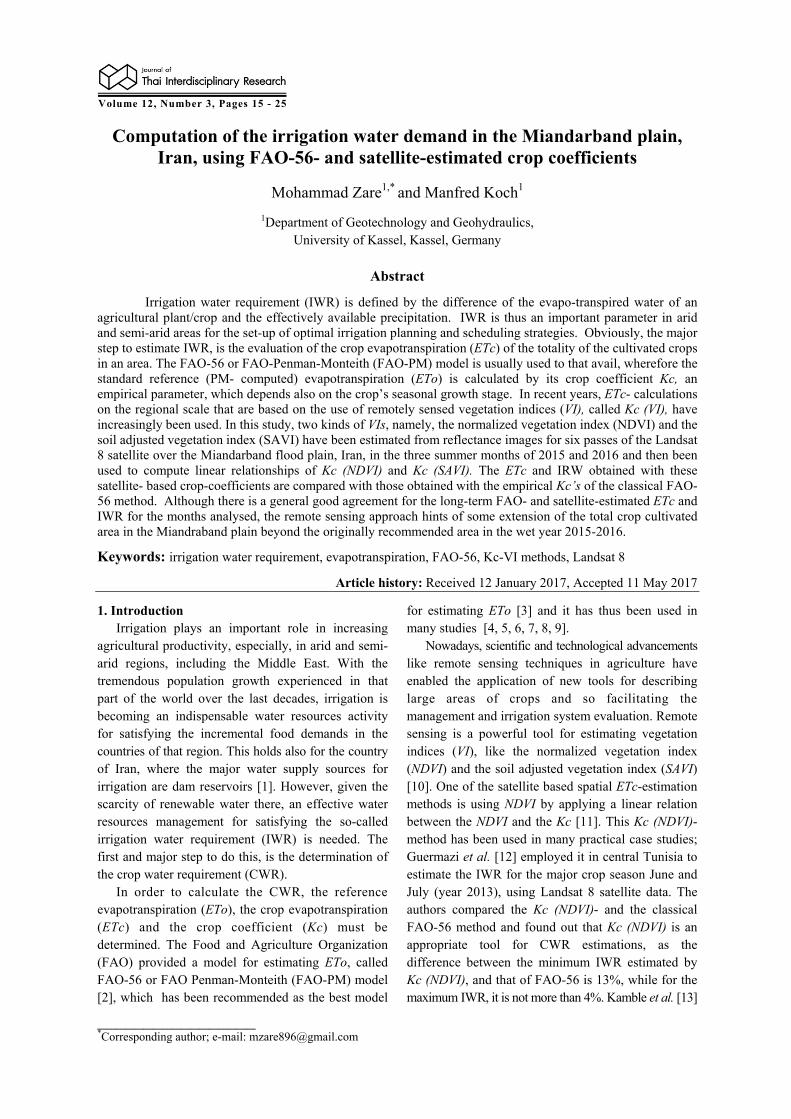
Figure 1 Miandarband plain in western Iran Table 1 Miandarband plain’s long-term average monthly values of various meteorological variables

Parameter Jan Feb Mar Apr May Jun Jul Aug Sep Oct Nov Dec P (mm) 62.2 56 76.3 64 28.8 1 0.4 0.3 2 28.7 56.2 59 Tmin (

oC) -3.5 -2.3 1.3 5.5 8.6 12.3 16.7 16 11.1 6.9 2.2 -1.4 Tmax (

oC) 7.6 9.9 14.9 20.3 26.4 33.8 38 37.5 32.9 25.5 16.6 10.4 RH (%) 72.2 66.6 58.3 55 46.3 27.1 21.9 21.4 24.1 37.9 58.8 69.4 Wind (m/s) 2.2 2.6 3.1 3.1 2.8 2.7 2.7 2.6 2.4 2.2 1.9 2 Sun (hours) 4.7 5.5 6.2 7 8.8 11.5 11.2 10.9 10.2 8 6.3 5

Table 2 Cultivation pattern and percentage of cultivated area (~200 km2) in the Miandarband plain

Crop Area (km2) Crop Area (km2) Crop Area (km2) Wheat 53.8 Clover 11.6 Apple 4 Alfalfa 27 Dry beans 11.5 Water melon 3.8 Barely 26.8 Chick beans 11.5 Tomato 3.8 Sweet corn 13.4 Sugar beet 9.6 Soybean 3.8 Field corn 11.6 Grape 4 Sun flower 3.8

estimated crop coefficients using the NDVI in three different locations for climate conditions in the High Plains in the Midwestern states of the US. They developed a simple linear regression model between the NDVI and the Kc using moderate resolution satellite data (MODIS) from the years 2006 and 2007. The results of these authors show that Kc- and NDVI- changes have a strong linear relation, with R2 = 0.9 and RMSE = 0.17, indicating that the Kc (NDVI)- equation is useful for irrigation planning. El-Shirbeny et al. [14] used the Kc (NDVI)- method in the Nile river valley down to the delta in Egypt to estimate ETc using Landsat 8 images in August 2013. Employing the FAO-56 method, the ETo were then calculated and the NDVI data applied to estimate the Kc and, subsequently, the ETc in the study area. In the present study the FAO-56 method is applied for ETc calculations in the Miandarband floodplain in western Iran which has been the focus of several recent studies of the authors [1, 15, 16] and then based on FAO-56 calculations high demand months during 2014 - 15 and 2015 - 16 water years (From October to

September in Iran) will be selected to ET estimation using the Kc-NDVI and Kc-SAVI models based on Landsat 8 satellite images. Finally, the efficiency of satellite-based model will be determined for IWR calculations. 2. Materials and methods 2.1 Study area and data The Miandarband plain is one of the most fertile plains of the Kermanshah province located in western Iran, between latitudes 34o 24’ 03’’ - 34o 40’ 56’’ and longitudes 46o 44’ 26’’ - 47o 11’ 00’’. (path/row: 167/36 for Landsat 8 satellite images). This region is geographically limited in the North by the Gharal and Baluch mountains and in the South by the Gharasoo river and has a surface area of about 300 km2 (see Figure 1). Surface water in the study area occurs in the form of springs and stream flow, with the major river being the Razavar river [15]. The plain is endowed in addition by ample groundwater resources, and with the construction of irrigation and drainage network,

Journal of Thai Interdisciplinary Research 17

Figure 2 Crop coefficient Kc–variations during a plant’s growing season [2] Table 3 Crop coefficients for the three stages of the growing season for the individual crops grown in the plain

Crop Kcin Kcmid Kcend Crop Kcin Kcmid Kcend Wheat 0.3 1.13 0.35 Sugar beet 0.35 1.20 0.70 Alfalfa 1.0 1.10 1.00 Grape 0.30 0.86 0.47 Barely 0.3 1.13 0.35 Apple 0.45 0.97 0.70 Sweet corn 0.3 1.20 0.55 Water melon 0.40 1.00 0.75 Field corn 0.3 1.16 1.10 Tomato 0.60 1.16 0.75 Clover 0.4 0.90 0.85 Soybean 0.40 1.16 0.60 Dry beans 0.4 1.16 0.50 Sun flower 0.35 1.08 0.50 Chick beans 0.4 1.00 0.57

it has become one of the high potential areas for crop production in recent years. It is expected that the irrigation and drainage network will convey about 176.2 MCM/year of surface water from the Gavoshan Dam into the Miandarband plain where it will be used for agricultural irrigation. The irrigation water management plan conceived by the ministry of power and ministry of agriculture since 1988, when the dam was constructed, and with the present day cultivation pattern (see below) suggested in 1995, plays a crucial role in the effective use of the available water resources [1]. It is estimated that 90% of the available water resources in the Miandarband plain are used for agriculture [17]. Meteorological data as well as cultivation pattern are required for IWR-calculation using the FAO-56 model. The long-term average monthly meteorological data includes precipitation (P), temperature (T), relative humidity (RH), wind speed and sun hours recorded over a period of 65 years (January 1951 to September 2016) in the area at one station are listed in Table 1. Whereas the precipitation data is used for defining the effective precipitation (Peff), the other parameters serve to compute the ETo by means of the CROPWAT 8.0 model. The cultivation pattern of the Miandarband plain is shown in Table 2. The cultivated area is about 200

km2 which means that 67% of the plain’s total surface is allocated to agricultural activities. 2.2 Water irrigation requirement (IWR) of original cultivation pattern in the Miandarband plain 1) Net irrigation requirement (NIR) computed by means of FAO-56 Penman-Monteith with empirical crop coefficients. The net irrigation requirement (NIR) describes the deficiency of water the crop needs for covering its crop evapotranspiration (ETc) needs and the available precipitation Peff. Thus the NIR is defined in FAO-56 model [2] is defined as:

effc PETNIR (1)

where

0ETKcETc (2)

i.e. the ETc is proportional to the reference crop evapotranspiration ETo. These equations are the basis of the FAO-56 model [2]. The Kc-values are not constant but change with the crop growth during the growing season. In this regard, each crop has three crop coefficients, namely, initial (Kcini), midseason (Kcmid) and late season (Kcend). The Kcini related to planting date covers up to 10% of the growth period, from 10% to 75% cover is called development and reaches then the crop coefficient Kcmid. Finally, Kcend

    18                                                                                                 Vol. 12 No. 3 May – June 2017

Table 4 Irrigation scheduling of crops Crop Jan Feb Mar Apr May Jun Jul Aug Sep Oct Nov Dec

Wheat & barely HD HD HD

Alfalfa HD HD HD Sweet & field corn HD HD HD Clover HD HD HD Dry beans HD HD HD Chick beans HD HD Sugar beet HD HD HD HD Grape HD HD HD Apple HD HD HD Water melon HD HD HD HD Tomato HD HD HD Soybean & Sun flower

HD HD HD

Irrigation months HD: IWR high demand months Growing season Table 5 CROPWAT 8.0 results for ETo (mm/month) and Rn (MJ m-2 day-1)

Parameter Jan Feb Mar Apr May Jun Jul Aug Sep Oct Nov Dec ET0 36.9 50.7 87.1 123.1 152.6 234.7 249.6 245.2 189.9 127.1 66 40.2 Rn 9.1 11.9 15.3 18.8 22.7 27.1 26.3 24.7 21.3 15.4 11 8.7

Table 6 Monthly IWR (MCM) values obtained with the FAO-56 method and using empirical crop coefficients, volumes of conveyed water (MCM) from the Gavoshan dam (CW), and the ensuing water deficit

Parameter Jan Feb Mar Apr May Jun Jul Aug Sep Oct Nov Dec IWR 0.1 1.2 3.9 13 29.3 66.7 65.8 55.1 21.7 7.6 1.4 0 CW 0.6 0 0.5 7 28 48 41.5 23.8 15.2 10.2 1.4 0 Water deficit 0 1.2 3.4 5 1.3 18.7 24.3 31.3 6.5 0 0 0

is related to the final growth period between maturity and senescence (see Figure 2). The Kc-values are taken from the FAO-56 paper (Table 12 in the FAO-56 guidelines, page 110). The tabular values (KcTab) listed there assume a RH of 45% and the wind speed taken 2m above surface (U2) is 2 m/s. This means that the data should be corrected by Eq. (3) in a particular application [2].

)(nStageKc

3.0min2))(( )

3)](45(004.0)2(04.0[

hRHUKc TabnStage (3)

where h is the plant height for each growth stage in m (0.1 m < h < 10 m). Using the equation above and the appropriate monthly values for RH and U2 in Table 2, the Kc- coefficients in each of the three stages of the growing season have been estimated for the various cultivated crops (see Tables 3 and 4). The Penman-Monteith (PM)-equation as implemented in FAO-56 [2] is used to estimate the daily reference evapotranspiration ETo (mm day-1 ):

2

2

34.01

273/900408.0

U

eeUTGRET asn

o

(4)

where Δ is the slope of the saturation vapour pressure curve (kPa/oC); Rn is net radiation at the crop surface (MJ m-2 day-1); G is the soil heat flux density (MJ m-2

day-1); γ is the psychometric constant (kPa/oC); T is average temperature (oC); and es-ea is the saturation vapour pressure deficit (kPa) (es = the saturation vapour pressure; ea = actual vapour pressure). By using the average monthly meteorological data of Table 1 and the altitude (1319 m), latitude and longitude (34.35 N and 47.15 E) of the meteorological station, the CROPWAT 8.0 model within the FAO-56 model is used to calculate Rn, depending only on the astronomical position of the sun, with G=0.04* Rn for a reference crop like alfafa and, finally, the daily ETo which has been summed up to one month in Table 5. Peff in Eq. (2) is estimated by the FAO/AGLW formula [18]:

0.6 10, 70 /

0.8 24, 70 / .eff

P for P mm monthP

P for P mm month

(5)

As a consequence of ongoing climate change in the region wherefore the annual precipitation in western Iran will be reduced between 9% to 28.5%, depending on the climate change scenario [19], Peff in the equation above has been multiplied by 0.8 in the NIR- formula (1). 2) IWR and water conveyance balance in the Miandarband plain

Journal of Thai Interdisciplinary Research 19

Using the relation between the NIR and IWR

eNIRIWR / (6)

where e is the total irrigation efficiency of the

irrigation system as well as the conveying and distribution efficiencies, the IWR is computed. In the study area surface irrigation is mainly used, for which a total efficiency of 50% has been recommended [17]. By multiplying the unit crop evapotranspiration ETc in Eq. (2) by the corresponding total cultivation area of that crop (see Table 2) and summing up for all crop areas, the total volumetric ETc is obtained. The latter, together with the value of the voluminous precipitation over the plain, are then used in Eqs. (1) and (6) to compute the monthly IWR-values. These are listed in Table 6, together the volumes of the monthly conveyed water from the Gavoshan dam (CW) and the difference between the two, the water deficit. The latter shows that for most of the months the water conveyed for irrigation is able to satisfy the IWR, giving some confidence on the irrigation management plan adopted. However, for months of June, July and August which are (seeผดิพลาด! ไม่พบแหล่ง

การอ้างองิ), on one hand the high demand- months for

most of the crops, being in the midseason or late season of their growing periods, while, on the other hand, the effective precipitation in this period is practical zero (see Table 1), the CW is not able to fulfil the IWR, so that groundwater must be used to avoid crop water stress conditions. 2.3 Determination of crop-coefficients from satellite remote sensing images The results of the application of the FAO-56 method to the Miandarband plain in the previous section are based on the cultivation pattern suggested by agricultural authorities some time ago. However, there is no data available to prove that farmers follow this cultivation pattern. In addition, the pattern is affected by natural hazards such as droughts which have been occurring with increasing frequency in recent years. Therefore, VI’s (vegetation indices) from satellite images could be a suitable tool to estimate the exact nature and cultivation areas of the crops, as well as the spatial distribution of the Kc-values. 1) NDVI- and SAVI- analysis of Landsat 8 images One of the high- resolution- and free-access satellite classes for retrieving VIs is the Landsat satellite family. The most recent one which was launched on February 11, 2013 is called Landsat 8. This satellite has 9 Operational Land Imager (OLI) spectral bands in the range 0.45 μm (blue/visible) to

2.29 μm (infrared/nonvisible) and 2 Thermal Infrared Sensor (TIRS) bands in the high infrared range (10 - 12.5 μm). Due to the relatively high horizontal resolution of the OLI bands (30 m), the frequent sweep of the satellite over the same corridor at the earth’s surface in intervals of 16 days, and the free availability of all data from the USGS (http://earthexplorer.usgs.gov), the Landsat 8 image data appears to be suitable for testing the Kc-NDVI regression method in the study region. For the retrieval of the NDVI which is of interest here, only two OLI-bands; the visible Red band 4 (centred around 0.65 μm) and the nonvisible Near-Infrared (NIR) band 5 (centred around 0.865 μm) are used. In the first processing step, the raw digital numbers (DN), defining the uncorrected

reflectance , are retrieved from the data archive for

one band and converted to Top of Atmosphere

(TOA)- Planetary Spectral Reflectance, by

correcting the former with the solar angle at the

time of the picture acquisition as:

sin/)*(sin/ pcalp AQM (7)

where, Qcal = DN denotes the raw digital number, MP is the reflectance multiplicative scaling factor, and AP is the reflectance. All these parameters are extracted from the metadata file downloaded with the DN data.

After conversion of the DN to reflectance ,

the vegetation indices (VIs) for the Red- and near-infrared (NIR) bands could be calculated. However, most of the VIs, including the already mentioned NDVI, the Soil Adjusted Vegetation Index (SAVI), which will also be used, the Weighted Difference Vegetation Index (WDVI), the Leaf Area Index (LAI), the Perpendicular Vegetation Index (PVI) and the Simple Ratio (SR) are based on the relative difference between the reflectance of the NIR- and Red bands. According to these statements, the NDVI is defined by the following equation [20]:

Re

Re

.NIR d

NIR d

NDVI

(8)

Based on this equation negative values of NDVI show water bodies and snow cover, whereas values greater than 0.5 show dense vegetation cover. Usually, it assumed that the NDVI- value for bare soil is near zero. The NDVI is sensitive to the soil background in partially vegetated pixels, i.e. for the same amount of vegetation cover the value of NDVI in darker

    20                                                                                                 Vol. 12 No. 3 May – June 2017

Figure 3 Left panel: scatter plot of NIR-Red band reflectance values with the regression-computed soil line for the August 12, 2016 satellite pass. Right panel: schematic sketch of the various bands running parallel to

the soil line and defining specific soil and vegetation conditions as indicated

 

Figure 4 NDVI (left panel) and SAVI (right panel) for the August 12, 2016, Landsat 8 pass substrates soils is higher than bright soils, thus using a VI which  suppresses the effects of soil brightness is desirable. In order to eliminating the soil background effects, the SAVI which is based on soil line concept has been applied. The soil line is a linear relation

between the reflectance of the NIR ( NIR ) and the

Red ( dRe ) bands for bare soil, is derived [21]:

0Re1 dNIR (9)

where 0 is the intercept and 1 is the slope of the

soil line. By plotting the value of the NIR reflectance in each pixel versus that of the Red one, a triangle-shaped plot, as shown in the left panel of for the Landsat image of the satellite’s pass on August 12, 2016, is obtained. As indicated in the right panel of that figure, parallel to the soil line running bands

within this triangle define specific soil and vegetation conditions, including the soil moisture content of each pixel [22]. Basically, on notice that the stronger is the vegetation cover, the higher are the NIR- and Red- reflectances. The lower enveloping soil line of the pixel

scatter plot is defined by NIR ~ dRe or, more

specifically, when 0 < NIR - dRe < 0.05 in a pixel

[22]. Thus, in order to compute the soil line here, all pixels falling in this range have been extracted first and then Eq. (9) is applied to compute the intercept

0 and slope 1 .

It should be noted that, in agreement with the

definition of the soil line, the 0 ’s and 1 ’s

computed for the various satellite images further down are indeed very close to 0 and 1, respectively.

Journal of Thai Interdisciplinary Research 21

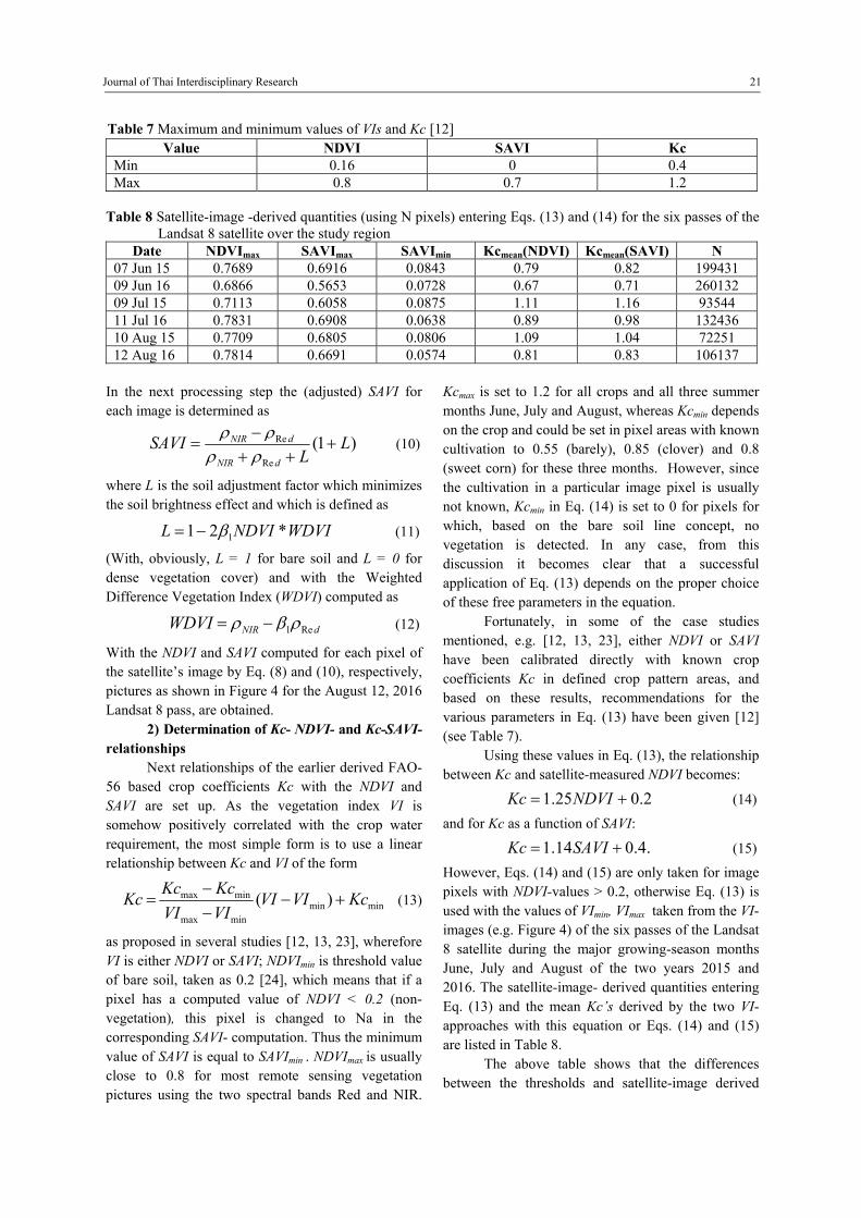
Value NDVI SAVI Kc

Min 0.16 0 0.4 Max 0.8 0.7 1.2

Table 8 Satellite-image -derived quantities (using N pixels) entering Eqs. (13) and (14) for the six passes of the Landsat 8 satellite over the study region

Date NDVImax SAVImax SAVImin Kcmean(NDVI) Kcmean(SAVI) N 07 Jun 15 0.7689 0.6916 0.0843 0.79 0.82 199431 09 Jun 16 0.6866 0.5653 0.0728 0.67 0.71 260132 09 Jul 15 0.7113 0.6058 0.0875 1.11 1.16 93544 11 Jul 16 0.7831 0.6908 0.0638 0.89 0.98 132436 10 Aug 15 0.7709 0.6805 0.0806 1.09 1.04 72251 12 Aug 16 0.7814 0.6691 0.0574 0.81 0.83 106137

In the next processing step the (adjusted) SAVI for each image is determined as

)1(Re

Re LL

SAVIdNIR

dNIR

(10)

where L is the soil adjustment factor which minimizes the soil brightness effect and which is defined as

WDVINDVIL *21 1            (11)

(With, obviously, L = 1 for bare soil and L = 0 for dense vegetation cover) and with the Weighted Difference Vegetation Index (WDVI) computed as

dNIRWDVI Re1              (12)

With the NDVI and SAVI computed for each pixel of the satellite’s image by Eq. (8) and (10), respectively, pictures as shown in Figure 4 for the August 12, 2016 Landsat 8 pass, are obtained. 2) Determination of Kc- NDVI- and Kc-SAVI- relationships Next relationships of the earlier derived FAO-56 based crop coefficients Kc with the NDVI and SAVI are set up. As the vegetation index VI is somehow positively correlated with the crop water requirement, the most simple form is to use a linear relationship between Kc and VI of the form

minminminmax

minmax )( KcVIVIVIVI

KcKcKc

(13)

as proposed in several studies [12, 13, 23], wherefore VI is either NDVI or SAVI; NDVImin is threshold value of bare soil, taken as 0.2 [24], which means that if a pixel has a computed value of NDVI < 0.2 (non-vegetation), this pixel is changed to Na in the corresponding SAVI- computation. Thus the minimum value of SAVI is equal to SAVImin . NDVImax is usually close to 0.8 for most remote sensing vegetation pictures using the two spectral bands Red and NIR.

Kcmax is set to 1.2 for all crops and all three summer months June, July and August, whereas Kcmin depends on the crop and could be set in pixel areas with known cultivation to 0.55 (barely), 0.85 (clover) and 0.8 (sweet corn) for these three months. However, since the cultivation in a particular image pixel is usually not known, Kcmin in Eq. (14) is set to 0 for pixels for which, based on the bare soil line concept, no vegetation is detected. In any case, from this discussion it becomes clear that a successful application of Eq. (13) depends on the proper choice of these free parameters in the equation. Fortunately, in some of the case studies mentioned, e.g. [12, 13, 23], either NDVI or SAVI have been calibrated directly with known crop coefficients Kc in defined crop pattern areas, and based on these results, recommendations for the various parameters in Eq. (13) have been given [12] (see Table 7). Using these values in Eq. (13), the relationship between Kc and satellite-measured NDVI becomes:

2.025.1 NDVIKc (14)

and for Kc as a function of SAVI:

1.14 0.4.Kc SAVI (15)

However, Eqs. (14) and (15) are only taken for image pixels with NDVI-values > 0.2, otherwise Eq. (13) is used with the values of VImin, VImax taken from the VI- images (e.g. Figure 4) of the six passes of the Landsat 8 satellite during the major growing-season months June, July and August of the two years 2015 and 2016. The satellite-image- derived quantities entering Eq. (13) and the mean Kc’s derived by the two VI- approaches with this equation or Eqs. (14) and (15) are listed in Table 8. The above table shows that the differences between the thresholds and satellite-image derived

Table 7 Maximum and minimum values of VIs and Kc [12]

    22                                                                                                 Vol. 12 No. 3 May – June 2017

Figure 5 Photos from March 29, 2016, showing the water logging problem in the Miandarband plain

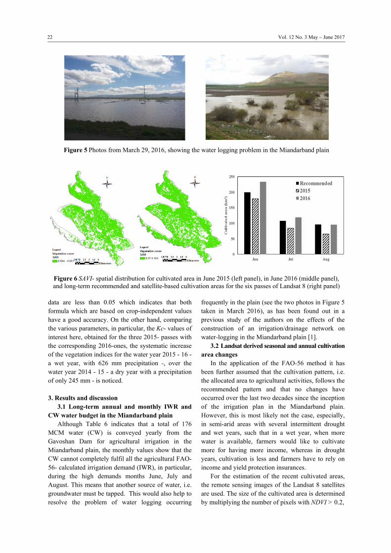
Figure 6 SAVI- spatial distribution for cultivated area in June 2015 (left panel), in June 2016 (middle panel), and long-term recommended and satellite-based cultivation areas for the six passes of Landsat 8 (right panel)

data are less than 0.05 which indicates that both formula which are based on crop-independent values have a good accuracy. On the other hand, comparing the various parameters, in particular, the Kc- values of interest here, obtained for the three 2015- passes with the corresponding 2016-ones, the systematic increase of the vegetation indices for the water year 2015 - 16 - a wet year, with 626 mm precipitation -, over the water year 2014 - 15 - a dry year with a precipitation of only 245 mm - is noticed. 3. Results and discussion 3.1 Long-term annual and monthly IWR and CW water budget in the Miandarband plain Although Table 6 indicates that a total of 176 MCM water (CW) is conveyed yearly from the Gavoshan Dam for agricultural irrigation in the Miandarband plain, the monthly values show that the CW cannot completely fulfil all the agricultural FAO-56- calculated irrigation demand (IWR), in particular, during the high demands months June, July and August. This means that another source of water, i.e. groundwater must be tapped. This would also help to resolve the problem of water logging occurring

frequently in the plain (see the two photos in Figure 5 taken in March 2016), as has been found out in a previous study of the authors on the effects of the construction of an irrigation/drainage network on water-logging in the Miandarband plain [1]. 3.2 Landsat derived seasonal and annual cultivation area changes In the application of the FAO-56 method it has been further assumed that the cultivation pattern, i.e. the allocated area to agricultural activities, follows the recommended pattern and that no changes have occurred over the last two decades since the inception of the irrigation plan in the Miandarband plain. However, this is most likely not the case, especially, in semi-arid areas with several intermittent drought and wet years, such that in a wet year, when more water is available, farmers would like to cultivate more for having more income, whereas in drought years, cultivation is less and farmers have to rely on income and yield protection insurances. For the estimation of the recent cultivated areas, the remote sensing images of the Landsat 8 satellites are used. The size of the cultivated area is determined by multiplying the number of pixels with NDVI > 0.2,

Journal of Thai Interdisciplinary Research 23

Figure 7 Left panel: Average areal monthly ETc for FAO- long-term recommended and satellite based cultivation areas for the six passes of Landsat 8 in 2015 and 2016; Right panel: Corresponding IWR

the threshold value indicating vegetation, by the unit areal resolution of one pixel (900 m2). Examples of two SAVI- spatial distributions computed with the images of the two passes of the satellite in June 2015 and June 2016 and used for these vegetation-area computations are shown in the two left panels of Figure 6. The results of this cultivated- area estimation for all six passes of the satellite are shown in the right panel of Figure 6, together with the areas of the recommended cultivated pattern estimated from the harvesting sequence of the various crops over the summer months [17]. One may notice, firstly and expectedly, that the cultivation areas in the pre-harvest season of the summer months of the wet year 2016 are higher than those for the dry year 2015 (which can also be noticed from the two SAVI- images of Figure 6), and, secondly, that farmers are trying, whenever the climate conditions permit, to increase the cultivated area beyond the original recommended one, such as in 2016. The barplot of Figure 6 shows also the effects of the harvesting in reducing the remotely sensed vegetation areas as the latter decrease from June to July when wheat, barely and chick beans, and, further, in August, when clover is harvested. 3.3 Evaluation of the crop evapotranspiration ETc using FAO- empirical and satellite-derived Kc’s Using (1) the empirical Kc-values with the recommended crop areas of Table 2 and, (2) the satellite-based average Kc’s of Table 8 for the whole cultivated area for each of the 6 passes of Landsat 8, in the FAO-56 crop evapotranspiration formula (Eq.2), the changes in the ETc’s between the historically recommended and the recently observed satellite-derived cultivation pattern can be estimated. However, as it can be inferred from Table 8 that the differences between Kc (NDVI) and Kc (SAVI) are

only minor, and since Kc (SAVI) is usually considered to be more reliable when bare soils are present, for visual simplification, we show these calculations for the satellite-based ETc’s only with Kc (SAVI). The results are shown in the left panel of Figure. 7. One can notice from the left panel of Figure 7 that for the same summer month, the differences in the total ETcs for the cultivated area are only minor. However, this does not hold for the wet year 2015 - 16, when the ETC in July, 2016 is significantly lower than that obtained for the original recommended cultivation pattern, notwithstanding the fact that Figure 6 showed that the total cultivated area had increased in that year. The reason for this discrepancy could be the related to the types of crops grown in that year and which are not recognizable in an unambiguous manner with satellite remote sensing. Multiplying these estimated ETc- values by the corresponding total areas of cultivation in the corresponding time period of one month (taken from values of the right panel of Figure 6), the total IWR is computed. The results are depicted in the right panel of Figure 7 from which one can notice that the satellite-based IWR is very close to the long-term IWR obtained for the recommended cultivation pattern (see Table 6) in June and July, but not in August, the latter being also the month experiencing the largest water deficit (see Table 6). 4. Conclusions Nowadays, agricultural development is one of the most important criteria for food security and can be a critical index for economic developments, particularly, in semi-arid regions, which are facing increasing water scarcity problems. This adverse situation is further exacerbated by climate changes effects, which requires better effective water management policies to overcome the conflict of water scarcity and more crop

    24                                                                                                 Vol. 12 No. 3 May – June 2017

yield. One of these policies consists in the construction of dams and conveying water to irrigation networks to fulfil the local crop water demands. Such is the case for the agriculturally heavily used Miandraband flood plain, western Iran, which is irrigated by water from the Gavoshan dam, constructed some 25 years ago. In spite of the high volumes of water stored by this dam, further agricultural development in the plain needs an optimal use of the limited amount of irrigation water conveyed. Calculation of the irrigation water requirement (IWR) calculation is a first step for achieving this objective. In this study, the FAO-56 crop evapotranspiration method, using (1) empirical crop coefficients Kc of the prevailing crops in the area, and (2) average Kc derived from remotely sensed vegetation- indices (VI), namely, Kc (NDVI) and Kc (SAVI), of 6 passes of the Landsat 8 satellite are employed in the IWR- calculation. The results indicate that these remotely sensed crop coefficients are not only useful to estimate the IWR, but also to detect temporal changes in the total area cultivated. Thus it was found that farmers have actually extended the total crop cultivation area in the Miandraband plain beyond the originally recommended area in the relatively wet water year 2015 - 2016. Although more research with regard to a better understanding of the individual relationship of the satellite-measured VI and a particular agricultural crop and, especially, it’s Kc is needed, the remote sensing analysis carried out here appears to be a suitable tool for irrigation water management in a cultivated area as a whole and is so able to complement classical FAO-56 crop water requirement calculations. References [1] Zare M, Koch M. 3D-groundwater flow modeling

of the possible effects of the construction of an irrigation/drainage network on water-logging in the Miandarband plain, Iran. Basic Research Journal of Soil and Environmental Science. 2014; 2 (3): 29-39.

[2] Allen RG, Pereira LS, Raes D, Smith M. Crop evapotranspiration-Guidelines for computing crop water requirements-FAO Irrigation and drainage paper 56. FAO, Rome. 1998; 300 (9): D05109.

[3] Djaman K, Irmak S, Kabenge I, Futakuchi K. Evaluation of FAO-56 Penman-Monteith Model with Limited Data and the Valiantzas Models for Estimating Grass-Reference Evapotranspiration in Sahelian Conditions. Journal of Irrigation and Drainage Engineering. 2016; 142 (11): 04016044.

[4] Anderson RG, Alfieri JG, Tirado-Corbalá R, Gartung J, McKee LG, Prueger JH. Assessing FAO-56 dual crop coefficients using eddy covariance flux partitioning. Agricultural Water Management; 2016.

[5] Connan O, Maro D, Hébert D, Solier L, Caldeira Ideas P, Laguionie P, et al. In situ measurements of tritium evapotranspiration (3H-ET) flux over grass and soil using the gradient and eddy covariance experimental methods and the FAO-56 model. Journal of Environmental Radioactivity. 2015; 148: 1-9.

[6] Farg E, Arafat SM, Abd El-Wahed MS, El-Gindy AM. Estimation of Evapotranspiration ETc and Crop Coefficient Kc of Wheat, in south Nile Delta of Egypt Using integrated FAO-56 approach and remote sensing data. The Egyptian Journal of Remote Sensing and Space Science. 2012; 15 (1): 83-89.

[7] Jabloun M, Sahli A. Evaluation of FAO-56 methodology for estimating reference evapotranspiration using limited climatic data:Application to Tunisia. Agriculture Water Management. 2008; 95 (6): 707-715.

[8] Malamos N, Barouchas PE, Tsirogiannis IL, Liopa-Tsakalidi A, Koromilas T. Estimation of Monthly FAO Penman-Monteith Evapotranspiration in GIS Environment, through a Geometry Independent Algorithm. Agriculture and Agricultural Science Procedia. 2015; 4: 290-299.

[9] Valiantzas JD. Simplified forms for the standardized FAO-56 Penman–Monteith reference evapotranspiration using limited weather data. Journal of Hydrology. 2013; 505: 13-23.

[10] Yi Q-x, Bao A-m, Wang Q, Zhao J. Estimation of leaf water content in cotton by means of hyperspectral indices. Computers and Electronics in Agriculture. 2013; 90: 144-151.

[11] Casa R, Rossi M, Sappa G, Trotta A. Assessing Crop Water Demand by Remote Sensing and GIS for the Pontina Plain, Central Italy. Water Resources Management. 2009; 23 (9): 1685-1712.

[12] Guermazi E, Bouaziz M, Zairi M. Water irrigation management using remote sensing techniques: a case study in Central Tunisia. Environmental Earth Sciences. 2016; 75 (3): 202.

[13] Kamble B, Kilic A, Hubbard K. Estimating Crop Coefficients Using Remote Sensing-Based Vegetation Index. Remote Sensing. 2013; 5 (4).

[14] El-Shirbeny M, Ali A, Saleh N. Crop Water Requirements in Egypt Using Remote Sensing Techniques. Journal of Agricultural Chemistry and Environment. 2014; 3: 57-65.

[15] Zare M, Koch M. Using ANN and ANFIS Models for simulating and predicting Groundwater Level Fluctuations in the Miandarband Plain, Iran. 4th IAHR Europe Congress;July 27-29; Liege, Belgium 2016.

Journal of Thai Interdisciplinary Research 25

[16] Ghobadian R, Mohamadi S, Golzari S. Numerical analysis of slid gate and neyrpic module intakes outflows in unsteady flow conditions. Ain Shams Engineering Journal. 2014; 5 (3): 657-666.

[17] Anonymous. Miandarband and Bilehvar irrigation and drainage network, final report. Mahab Ghods Co, (in Farsi); 2001.

[18] Smith M. Manual for CROPWAT version 5.2. FAO, Rome. 45 pp. 1988.

[19] Fattahi E, Habibi M, Kouhi M. Climate Change Impact on Drought Intensity and Duration in West of Iran. Journal of Earth Science and Climatic Change. 2015; 6 (319).

[20] Ozelkan E, Chen G, Ustundag BB. Multiscale object-based drought monitoring and comparison in rainfed and irrigated agriculture from Landsat 8 OLI imagery. International Journal of Applied Earth Observation and Geoinformation. 2016; 44: 159-170.

[21] Fox GA, Sabbagh GJ, Searcy SW, Yang C. An Automated Soil Line Identification Routine for Remotely Sensed Images. Soil Science Society of America Journal. 2004; 68 (4): 1326-1331.

[22] Amani M, Parsian S, MirMazloumi SM, Aieneh O. Two new soil moisture indices based on the NIR-red triangle space of Landsat-8 data. International Journal of Applied Earth Observation and Geoinformation. 2016; 50: 176-186.

[23] Rafn E, Contor B, Ames D. Evaluation of a Method for Estimating Irrigated Crop-Evapotranspiration Coefficients from Remotely Sensed Data in Idaho. Journal of Irrigation and Drainage Engineering. 2008; 134 (6): 722-729.

[24] Sobrino JA, Jiménez-Muñoz JC, Paolini L. Land surface temperature retrieval from LANDSAT TM 5. Remote Sensing of Environment. 2004; 90 (4): 434-440.