computation in the wild: reconsidering dynamic systems in
TRANSCRIPT
Computation in the Wild: Reconsidering Dynamic Systems
in Light of Irregularity
by
Tony Liu
A thesis submitted in partial fulfillment
of the requirements for the
Degree of Bachelor of Arts with Honors
in Computer Science
Williams College
Williamstown, Massachusetts
May 2, 2016

Contents
1 Introduction 1
2 Previous Work 3
2.1 Motivation and Applications . . . . . . . . . . . . . . . . . . . . . . . . 3
2.1.1 Cellular Automata for Biological Modeling: Stomatal Patchiness 3
2.1.2 CA Models of Social and Ecological Dynamics . . . . . . . . . . 4
2.1.3 Cellular Automata as Inspiration for Novel Computing Models . 5
2.2 Criticality and the Emergence of Computation . . . . . . . . . . . . . . 6
2.2.1 Foundations of Computation in Dynamical Systems . . . . . . . 6
2.2.2 Metrics . . . . . . . . . . . . . . . . . . . . . . . . . . . . . . . . 6
2.2.3 The Edge of Chaos: Investigating where Computation Emerges . 8
2.3 Robustness in Face of Irregularity . . . . . . . . . . . . . . . . . . . . . . 10
2.3.1 Stomatal Dynamics Revisited: Utilizing Environmental Noise . . 10
2.3.2 Redundancy in Decentralized Systems . . . . . . . . . . . . . . . 11
2.4 Spatial Representations and Modeling of CAs . . . . . . . . . . . . . . . 13
2.4.1 Limitations of Traditional CA Spatial Representations . . . . . . 13
2.4.2 Spatial Variation of Conway’s Game of Life . . . . . . . . . . . . 13
2.4.3 Voronoi Representations of CA . . . . . . . . . . . . . . . . . . . 14
2.5 Summary . . . . . . . . . . . . . . . . . . . . . . . . . . . . . . . . . . . 15
3 System Design 23
3.1 System Overview . . . . . . . . . . . . . . . . . . . . . . . . . . . . . . . 23
3.1.1 Structures . . . . . . . . . . . . . . . . . . . . . . . . . . . . . . . 24
3.1.2 Input/Output Files and Running Our System . . . . . . . . . . . 24
3.2 Grid Generation . . . . . . . . . . . . . . . . . . . . . . . . . . . . . . . 24
3.2.1 Penrose Tilings . . . . . . . . . . . . . . . . . . . . . . . . . . . . 25
3.2.2 Delaunay Triangulations and Voronoi Diagrams . . . . . . . . . . 25
3.2.3 Voronoi Quadrilaterals . . . . . . . . . . . . . . . . . . . . . . . . 26
3.3 Grid Degeneration . . . . . . . . . . . . . . . . . . . . . . . . . . . . . . 26
3.3.1 Generator Point Removal . . . . . . . . . . . . . . . . . . . . . . 26
3.3.2 Crosshatching Degeneration . . . . . . . . . . . . . . . . . . . . . 26
3.4 Stencil and Rule Table Implementation . . . . . . . . . . . . . . . . . . 27
3.4.1 Generalized von Neumann and Moore Neighborhoods . . . . . . 27
3.4.2 Game of Life Rule Tables . . . . . . . . . . . . . . . . . . . . . . 27
i
3.4.3 � Rule Tables . . . . . . . . . . . . . . . . . . . . . . . . . . . . . 28
3.5 Summary . . . . . . . . . . . . . . . . . . . . . . . . . . . . . . . . . . . 28
4 Penrose Life Experiments 36
4.1 Lifetime to Stability and Ash Density . . . . . . . . . . . . . . . . . . . 36
4.2 Single Run Analysis . . . . . . . . . . . . . . . . . . . . . . . . . . . . . 37
4.3 Neighborhood Analysis . . . . . . . . . . . . . . . . . . . . . . . . . . . . 38
4.4 Subregion Analysis . . . . . . . . . . . . . . . . . . . . . . . . . . . . . . 39
4.5 Potential for Penrose Gliders . . . . . . . . . . . . . . . . . . . . . . . . 40
4.6 Summary . . . . . . . . . . . . . . . . . . . . . . . . . . . . . . . . . . . 41
5 Local Majority Experiments 57
5.1 Baseline Majority Task Performance on Irregular Grids . . . . . . . . . 57
5.2 Majority Task Performance with State Noise . . . . . . . . . . . . . . . 58
5.3 Summary . . . . . . . . . . . . . . . . . . . . . . . . . . . . . . . . . . . 59
6 Lambda Degradation Experiments 68
6.1 The Langton-Wootters � Profile . . . . . . . . . . . . . . . . . . . . . . 68
6.2 � Profile of Irregular Grids . . . . . . . . . . . . . . . . . . . . . . . . . 69
6.3 � Profile of Degenerated Grids . . . . . . . . . . . . . . . . . . . . . . . 71
6.3.1 Generator Point Degeneration . . . . . . . . . . . . . . . . . . . . 71
6.3.2 Crosshatching Degeneration . . . . . . . . . . . . . . . . . . . . . 72
6.4 Summary . . . . . . . . . . . . . . . . . . . . . . . . . . . . . . . . . . . 73
7 Future Work 90
7.1 Evaluation and Critique of Our Results . . . . . . . . . . . . . . . . . . 90
7.2 Measuring Information Transfer . . . . . . . . . . . . . . . . . . . . . . . 91
7.3 Consideration of Continuous Dynamical Systems . . . . . . . . . . . . . 92
7.4 Criticality under Microscope: Other CA Metrics to Consider . . . . . . 92
8 Conclusions 97
Appendix A Definitions of Criticality Metrics 99
A.1 Lambda . . . . . . . . . . . . . . . . . . . . . . . . . . . . . . . . . . . . 99
A.2 Gamma . . . . . . . . . . . . . . . . . . . . . . . . . . . . . . . . . . . . 99
A.3 Shannon Entropy . . . . . . . . . . . . . . . . . . . . . . . . . . . . . . . 100
A.4 Mutual Information . . . . . . . . . . . . . . . . . . . . . . . . . . . . . 100
A.5 Mean Field Theory Estimates . . . . . . . . . . . . . . . . . . . . . . . . 100
Appendix B Supplementary Calculations 103
B.1 Calculating Unique Rotations in a � Transition Table . . . . . . . . . . 103
B.2 Maximum Entropy and � for K=8, N=5 CA . . . . . . . . . . . . . . . . 103
ii

List of Figures
2.1 Majority Task CA . . . . . . . . . . . . . . . . . . . . . . . . . . . . . . 16
2.2 Qualitative CA-Stomata Comparison . . . . . . . . . . . . . . . . . . . . 16
2.3 CA Neighborhood Stencils . . . . . . . . . . . . . . . . . . . . . . . . . . 16
2.4 Wolfram’s Complexity Classes . . . . . . . . . . . . . . . . . . . . . . . . 17
2.5 Ordered CA Transient Length . . . . . . . . . . . . . . . . . . . . . . . . 17
2.6 Chaotic CA Transient Length . . . . . . . . . . . . . . . . . . . . . . . . 18
2.7 Complex CA Transient Length . . . . . . . . . . . . . . . . . . . . . . . 19
2.8 Lambda and Transient Length . . . . . . . . . . . . . . . . . . . . . . . 20
2.9 Hypothesized CA Space . . . . . . . . . . . . . . . . . . . . . . . . . . . 20
2.10 Filtered CA Behavior . . . . . . . . . . . . . . . . . . . . . . . . . . . . 21
2.11 Voronoi Diagram . . . . . . . . . . . . . . . . . . . . . . . . . . . . . . . 21
2.12 “Dead Cells” in Voronoi CA . . . . . . . . . . . . . . . . . . . . . . . . . 22
3.1 CA Simulation Platform Architecture . . . . . . . . . . . . . . . . . . . 29
3.2 Representative Grid Data File . . . . . . . . . . . . . . . . . . . . . . . . 30
3.3 Random Point Generation . . . . . . . . . . . . . . . . . . . . . . . . . . 31
3.4 Voronoi Diagram Generation . . . . . . . . . . . . . . . . . . . . . . . . 32
3.5 Voronoi Quad Generation . . . . . . . . . . . . . . . . . . . . . . . . . . 32
3.6 Voronoi Quad Grid . . . . . . . . . . . . . . . . . . . . . . . . . . . . . . 33
3.7 Generator Point Degradation . . . . . . . . . . . . . . . . . . . . . . . . 34
3.8 Crosshatching Degeneration . . . . . . . . . . . . . . . . . . . . . . . . . 35
3.9 Game of Life Rule Table . . . . . . . . . . . . . . . . . . . . . . . . . . . 35
4.1 Circular Penrose Tilings . . . . . . . . . . . . . . . . . . . . . . . . . . . 42
4.2 Kite/Dart Lifetime and Ash Density Graphs . . . . . . . . . . . . . . . . 43
4.3 Hill et al.’s Kite/Dart Lifetime and Ash Density Graphs . . . . . . . . . 44
4.4 Hill et al.’s Standard GoL Lifetime and Ash Density Graphs . . . . . . . 45
4.5 Rhomb Lifetime and Ash Density Graphs . . . . . . . . . . . . . . . . . 46
4.6 Kite/Dart and Rhomb Lifetime Graph . . . . . . . . . . . . . . . . . . . 47
4.7 Kite/Dart Single Run Density Graph . . . . . . . . . . . . . . . . . . . . 47
4.8 Rhomb Single Run Sequence . . . . . . . . . . . . . . . . . . . . . . . . 50
4.9 Rhomb Single Run Density Graph . . . . . . . . . . . . . . . . . . . . . 51
4.10 Generalized Moore Neighborhoods for Kites/Darts and Rhombs . . . . . 51
4.11 Kite/Dart and Rhomb Neighborhood Size Frequency . . . . . . . . . . . 52
iii

4.12 Rhomb Single Run Neighborhood ON Percentage . . . . . . . . . . . . . 52
4.13 Kite/Dart and Rhomb Average Neighborhood Size . . . . . . . . . . . . 52
4.14 Rhomb Subregion Initialization . . . . . . . . . . . . . . . . . . . . . . . 53
4.15 Small/Large Lifetime Graphs . . . . . . . . . . . . . . . . . . . . . . . . 54
4.16 Subregion Ash Density Plots . . . . . . . . . . . . . . . . . . . . . . . . 55
4.17 Penrose Glider . . . . . . . . . . . . . . . . . . . . . . . . . . . . . . . . 56
5.1 Irregular Delaunay Grid for Majority Task . . . . . . . . . . . . . . . . . 61
5.2 Grid Generation from Stomatal Array . . . . . . . . . . . . . . . . . . . 62
5.3 Replication of Messinger et al.’s Baseline Local Majority Performance . 63
5.4 Local Majority Task Performance on Irregular Grids . . . . . . . . . . . 64
5.5 Local Majority Task Performance on a Non-Periodic Regular Grid . . . 64
5.6 Local Majority Task Performance for Regular Grids with Noise . . . . . 65
5.7 Local Majority Task Performance for the Stoma Grid with Noise . . . . 66
5.8 Local Majority Task Performance on “Hard” Configurations . . . . . . . 67
6.1 The Langton-Wootters Profile . . . . . . . . . . . . . . . . . . . . . . . . 75
6.2 VQuad Generation from Stomatal Array . . . . . . . . . . . . . . . . . . 76
6.3 Langton-Wootters Profile for Short and Long Simulations . . . . . . . . 77
6.4 Voronoi Quad Langton-Wootters Profile . . . . . . . . . . . . . . . . . . 78
6.5 Stoma Langton-Wootters Profile . . . . . . . . . . . . . . . . . . . . . . 79
6.6 Penrose Langton-Wootters Profile . . . . . . . . . . . . . . . . . . . . . . 80
6.7 Stomatal Generator Point Degeneration . . . . . . . . . . . . . . . . . . 81
6.8 Langton-Wootters Profile for Generator Point Degeneration . . . . . . . 82
6.9 Crosshatch Degeneration, w = 10 . . . . . . . . . . . . . . . . . . . . . . 83
6.10 Crosshatch Degeneration, w = 20 . . . . . . . . . . . . . . . . . . . . . . 84
6.11 Crosshatch Degeneration, w = 30 . . . . . . . . . . . . . . . . . . . . . . 85
6.12 Crosshatch Langton-Wootters Profile, w = 10 . . . . . . . . . . . . . . . 86
6.13 Crosshatch Langton-Wootters Profile, w = 20 . . . . . . . . . . . . . . . 87
6.14 Crosshatch Langton-Wootters Profile, w = 30 . . . . . . . . . . . . . . . 88
6.15 Mean Squared Error for Crosshatching Degeneration . . . . . . . . . . . 89
7.1 SmoothLife Transition Rule . . . . . . . . . . . . . . . . . . . . . . . . . 94
7.2 Stomatal CA Power Law Correlation . . . . . . . . . . . . . . . . . . . . 95
7.3 Power Spectral Density for K=2, N=9 CAs . . . . . . . . . . . . . . . . 95
7.4 Attractor Basin Portraits . . . . . . . . . . . . . . . . . . . . . . . . . . 96
A.1 Mean Field Theory Lambda-Entropy Curve . . . . . . . . . . . . . . . . 102
iv

Abstract
Dynamic, spatially-oriented systems found in nature such as plant cell arrays or ant
colonies can produce complex behavior without centralized coordination or control. In-
stead, they communicate locally, with these local interactions producing emergent be-
havior globally across the entire system. The essence of these decentralized systems can
be captured utilizing cellular automata (CA) modeling, and such models are utilized for
investigating and simulating such natural systems. However, CA models assume spatial
regularity and structure, which are certainly not present in natural systems. In fact,
natural systems are inherently robust to spatial irregularities and environmental noise.
In this work, we relax the assumption of spatial regularity when considering cellular
automata in order to investigate the conditions in which complex behavior can emerge
in noisy, irregular natural systems.
v

Acknowledgments
I would like to thank Brent Heeringa for being my second reader, David Peak for pro-
viding both plant stomatal data and inspiration for this work, and Adly Templeton for
joining me on this exploration of the complexities of life, natural and artificial. Most
of all, I would like to thank Duane Bailey for being my advisor, for providing guidance
for this work and beyond over the years, and for being an unforgettable teller of stories.
Groovy.
vi

Chapter 1
Introduction
Dynamic natural systems have the ability to perform complex tasks that resemble com-
putation, often without the aid of a central processing unit. In particular, spatial systems
that are only locally connected, such as plant cell arrays or single-agent populations, can
produce emergent, globally-coordinated behavior [7, 34]. These systems are of particular
interest because of their massive parallelism and fault tolerance within noisy, imperfect
environments [47]. Decentralized dynamic systems can be described and modeled using
cellular automata (CA) because of a CA’s ability to support complex behavior arising
from simple components and strictly local connectivity [33]. The goal with CA models
is to able to examine how and under what conditions global, distributed computation
emerges in such systems.
One of the main motivating examples of emergent natural computation we have
been examining is plant cell stomatal coordination. These dynamic pores control gas
exchange within the plant and “solve” a constrained optimization problem without a
central communication system. What is remarkable about stomata is that their behav-
ior is statistically indistinguishable from the behavior of CAs that solve the majority
problem: a global coordination task where all cells in the CA need to converge to the
majority state of the initial configuration [34, 42, 48]. Furthermore, the corresponding
majority task automata have been shown to respond robustly in the face of variations
in their environment such as state noise, much like their biological counterparts [30].
This relationship is exciting because it has been shown that computation in CAs can
only occur under specific conditions, existing at a critical point between ordered and
chaotic behavior [26, 51]. Thus, perhaps we could begin to understand how computation
emerges in nature given their established connection with CAs. However, the automata
models built to study natural systems like plant stomata make a potentially limiting
assumption: regularity of both the cellular grid and the local connections. Dynamic
systems in nature certainly do not appear in a uniformly connected lattice. Like their
surrounding environment, the spatial orientation of these systems are noisy and prone
to irregularities. While some work investigates the e↵ects of nonuniform grids such as
Voronoi diagrams or Penrose tilings on automata performance [9, 17, 23], further study
is needed to ensure that our models of computation can safely be “mapped” to the
systems occurring in nature.
1
With these considerations in mind, this work pursues a deeper exploration of irregu-
lar computing CAs. Here, we conduct a series of experiments on a spectrum of automata
with irregular grids and connectivities, quantifying their behavior and comparing them
to traditional CAs. As noted earlier, computation appears to emerge at a point of
criticality somewhere in between the ordered and chaotic automata and Langton’s �
parameter, representing the relative order of a CA, is used to parametrize the possible
automata space [26]. � is important because it is an indicator of the class of CAs that
have the ability to compute [52]. However, this measure is tuned specifically for static
neighborhood definitions and uniform grids. With the experimentation on irregular au-
tomata, the goal is to explore and develop a more general notion of � and other metrics
so that we can better understand and perhaps even quantify the conditions in which
computation can emerge in noisy systems. Another important question we address with
this work is whether there is a qualitative di↵erence between regular and irregular grid
patterns and connectivities: are there cases where uniform CA models are su�cient for
representing biological systems?
We believe that the study of CA behavior in irregular environments is critical to
achieve a greater understanding of how biological systems combat imperfections. Ulti-
mately, the contribution of work on natural computational systems is twofold: not only
can we achieve a better understanding of how some biological processes operate, but
knowledge of how these systems work can inspire alternative computing methods [29, 46].
The hope is to illuminate how nature is able to perform complex computation in noisy
environments and apply these lessons to advance robust computing models.
We will begin with a review of previous work in Chapter 2, spanning the concepts
of criticality, robustness, and spatial representations in computing dynamic systems
and examining the potential applications of such models. We will describe our system
architecture in Chapter 3 as well as the tools we built to explore complex behavior in
CA systems. Experimental results will be presented in Chapters 4, 5, and 6, with future
work described in Chapter 7.
2

Chapter 2
Previous Work
Why are we interested in distributed computational CA systems? The goal is to achieve
a better understanding of how computation naturally emerges from such systems in order
to accurately model biological distributed processes as well as improve our technological
computing models. We will begin with some motivating examples by considering pre-
vious work on applications of robust, distributed CA models, spanning topics such as
plant biology, population dynamics, geographic modeling, and computer architecture.
However, in order to e↵ectively apply CA models of natural systems, we must under-
stand what computation means in such dynamic systems. Are there requisite properties
of computation and, if so, how do they arise? For this we consider a collection of pa-
pers that develop a framework for quantifying computational characteristics as well as
present a hypothesis that computation emerges at the “edge of chaos.” Next, as we
need to understand how natural computation is robust in the face of noisy and irreg-
ular environments, we will examine work on noise and fault tolerance in distributed
automata systems. Finally, spatial irregularity is a prevalent feature in nature that is
often overlooked in such studies, so we consider some work that examines the impact of
such irregularity on dynamic CA systems.
2.1 Motivation and Applications
2.1.1 Cellular Automata for Biological Modeling: Stomatal Patchiness
An important motivating example for this work is the modeling of plant cell stomatal
coordination done by Peak et al. Plant stomata are dynamic pores distributed across
leaves that control gas exchange by opening and closing their apertures. These stomata
are solving a constrained optimization problem: they maximize the uptake of CO2 while
minimizing water vapor loss [34, 48]. Long believed to be autonomous units that respond
similarly but independently to environmental conditions, it has now been shown that
a stoma’s aperture is also dependent on interactions with neighboring stomata, some-
times producing coordinated behavior called stomatal patchiness, where large groups of
stomata uniformly open or close [42]. This phenomenon is poorly understood by biol-
ogists, due to its apparent negative impact on gas exchange optimization as well as its
3
highly variable behavior. However, with biological evidence that plant stomata inter-
act locally [42], task-performing cellular automata are suitable candidates for modelling
patchy stomatal conductance. In fact, modeling has shown that the stomatal systems
are statistically indistinguishable from CAs configured to solve the majority task or
consensus problem, which involves determining which state (0 or 1, open or closed) is
the majority state in the initial configuration and then converging all cells to that state
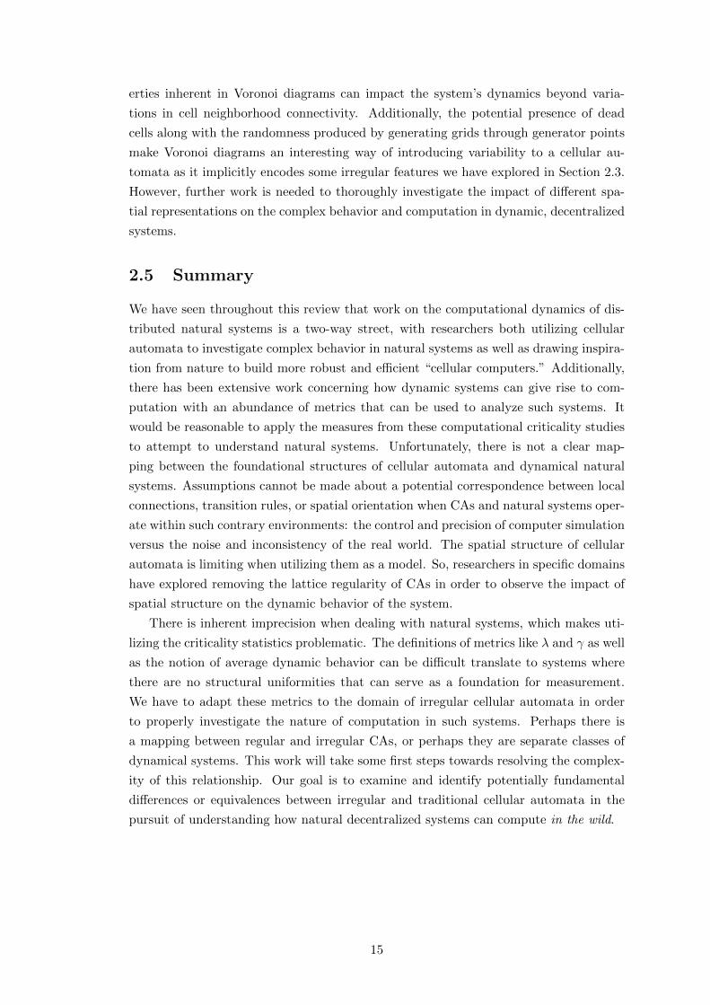
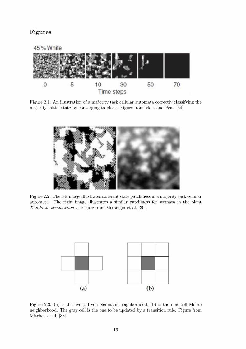
(Figure 2.1) [21]. Qualitative comparisons yield similarities to these task-performing au-
tomata as well (Figure 2.2). The patchiness observed in the plant stomata are analogous
to transient periods that are essential for the computation of majority in CAs. What is
remarkable about these stomatal systems is their response to irregularity, as they must
manage highly variable and imperfect environments. The corresponding majority task
CAs have been shown to respond robustly in the face of state noise, imperfect informa-
tion transfer, and transition rule heterogeneity. In fact, task performance seems to be
enhanced in some cases by the presence of noise [30].
It is important to note, however, that none of these systems are guaranteed to
optimally solve the majority task, and even determining whether or not a single instance
will perform optimally is hard. The inherent di�culty of determining the success or
failure of a given task-performing network emphasizes the importance of information
granularity: in an appeal to the concept of self-organizing criticality [5], small pieces of
fine grain information about initial configurations may lend more insight to the global
behavior of a distributed network than large but coarse bodies of information about
the structure of the space. Thus, studying stomatal patchiness not only provides a
step towards connecting computation to phenomenon in nature but also illustrates the
central ideas of robustness and criticality.
2.1.2 CA Models of Social and Ecological Dynamics
Researchers in ecology and the social sciences often use CA models when modeling
dynamics because automata models encapsulate essential features of many real-world
processes. The discrete and distributed nature of CA system provide a tractable system
where agents (represented by individual cells) can interact in local, overlapping neigh-
borhoods [7, 22]. In particular, the local interconnections present in cellular automata
models illuminate how micro-level rules can give rise to certain macro-level e↵ects, a cru-
cial aspect of domains such as population dynamics. Because the micro/macro relations
are readily apparent in CA systems, scientists in these fields can utilize such models
to not only produce quantitative simulations and predictions in but also to achieve a
qualitative understanding of how the real world operates [22]. Cellular automata are
appealing because they take a “simplistic” approach to “complex” modeling, which
not only is useful in domains where details on the underlying mechanisms are not well
understood (such as animal herd movement or forest fire behavior) but also reduces
multi-agent systems to their fundamental one-on-one interactions [7, 9], again allud-
ing to the importance of fine-grain information when trying to understand coarse-grain
processes.
4
Scientists in these fields recognize the limitations of CA models as well, as there are
concerns that the discrete and uniform nature of these systems are potentially prohibitive
in providing a su�ciently accurate representation of the real-world phenomena they are
trying to model. In particular, there is a need for variability in both the spatial con-
struction of the modeling environment as well as the local relationship between cells [17]
that the regular lattice structure of traditional cellular automata do not provide. We
will consider these limitations as well as work on alternative spatial configurations in
more detail in Section 2.4.
2.1.3 Cellular Automata as Inspiration for Novel Computing Models
Additionally, distributed CA systems have provided inspiration for new forms of com-
puting. Computing models based on cellular automata are founded upon three funda-
mental principles: simplicity, “vast parallelism”, and locality [47]. Similar to the appeal
of automata systems in dynamic modeling, CA-based computers utilize simple “cellu-
lar” computational units in tandem to solve complex computational tasks, can invoke
parallelism on a scale that traditional parallel systems cannot achieve, and have better
fault containment as well as more tolerance of imperfect input and execution due to
strictly local connectivity.
An example of such a cellular-based computing is the CAM-8 architecture developed
by Margolus. The CAM-8 computer architecture is motivated by the idea that in order to
maximize computational density, the underlying structure of the computer must mimic
the basic spatial locality of physical law [29]. Thus, the architecture is mesh network
of local CA compute nodes as they accurately represent the local interconnectivity that
is present in real-world micro-physical systems. As a result, there is a correspondence
between how computation is performed under the architecture and the physical imple-
mentation of the system itself. Because of this adherence to physical law, the CAM-8
architecture is particularly capable of computing spatially moving data, ideal for particle
simulation and medical imaging, among others [29]. The goal with CAM-8 and other
distributed cellular computing models is not necessarily to replace serial computers, but
rather to find particular domains of problems where these alternative computing models
can match and perhaps surpass the performance of traditional computing models.
These cellular-based computing architectures are not without limits. One of the
main challenges in cellular computing is being able to find local interaction rules that
express the overall problem that needs to be computed. There is no good way to abstract
beyond the local CA rules to provide a high-level interface for programmers to develop
in, making deliberate and controlled global behavior di�cult to produce. Indeed, this
is the main barrier CAM-8 must overcome in order to become a viable and practical
computer architecture. There is also an issue of scalability. Scaling grid size does not
necessarily bring about performance scaling or even task scaling: whether or not the
same level of performance on the task is maintained [47]. Nevertheless, the potential
applications in building cellular-based computational models illustrate the promise of
examining robust distributed computation in natural CA-like systems.
5
2.2 Criticality and the Emergence of Computation
2.2.1 Foundations of Computation in Dynamical Systems
What are the requisite conditions for computation to emerge from a dynamical system?
It has been shown that various CA systems can support universal computation [51],
but what are the particular characteristics that allow for computation to be possible?
Computational constructs such as Turing machines and other equivalent entities are
built upon three fundamentals that can be formulated in the dynamics of a CA system.
The system must be able to support the storage of information, with the ability to
preserve information for arbitrary time periods. Information transmission across long
distances must also be possible in the environment. Finally, there must be some mech-
anism for information interaction with the potential for information to be transformed
or modified [26]. These properties are necessary for any dynamical system, automata
or otherwise, to have the capacity for computation, but are not su�cient. Langton also
establishes the notion of dynamical systems undergoing “physical” phase transitions be-
tween highly ordered to highly disordered dynamics, with the most interesting behavior
occurring within the boundaries of this transition. This transition region is also where
the three requisite properties of computation often occur. Thus, the hypothesis Langton
claims is that computation can spontaneously emerge and dominate the dynamics of a
physical system when such a system is at or near such a critical transition point [26].
2.2.2 Metrics
Throughout the pursuit of understanding computation in dynamical CA systems, many
metrics have been utilized and created that can help quantify particular computational
characteristics. We will touch on and present some of them here, with equations listed
in Appendix A.
We will begin with a formal definition of a cellular automaton [26]. A CA is composed
of a lattice of dimension D with a finite automaton present in each cell of the lattice.
There is a finite neighborhood region N , where N = |N | is the number of cells covered
in the neighborhood region. Typical neighborhood stencils for two-dimensions are the
five-cell von Neumann neighborhood and the nine-cell Moore neighborhood (Figure 2.3).
Each cell contains a finite set of cell states ⌃ of size K = |⌃| and a transition function
� that maps a set of neighborhood configurations to the cell states: � : ⌃N ! ⌃. We
typically characterize a particular class of cellular automata by the number of neighbors
N and the number of cell states K.
Wolfram proposed a qualitative method for classifying CA automata behavior, with
systems falling into one of four classes [33, 50]:
• Class I: All initial configurations relax to the same fixed, homogeneous state.
• Class II: The CA relaxes to simple periodic structures, perhaps dependent on the
initial configuration.
• Class III: Most initial configurations degenerate to chaotic, unpredictable behavior.
6
• Class IV: Some initial configurations result in complex localized structures that
have the potential to be long-lived.
Li et al. later expands this list to six categories, with Class I and Class II split into
subclasses. Though these are broad, rough categorizations, we expect Class IV to be
the category of interest when examining potential capacity for computation in cellular
automata.
The parameter � (Appendix A.1) as established by Langton is used to both narrow
the space of CAs to consider as well as to measure the relative homogeneity or het-
erogeneity of a CA rule table: a completely homogeneous rule table maps all entries
to a single quiescent state whereas a completely heterogeneous rule table maps entries
to random states [26]. � is the fraction of the number of non-quiescent mappings in a
given rule table, and can be thought of the average amount of order a given automata
transition rule set possesses. Thus, � values range from 0, which represents a completely
homogeneous rule table to 1 � 1K
, which represents a completely heterogeneous table.
There is also a notion of critical �, denoted �c
, where the most complex dynamics tend
to emerge. Criticality will be examined in more detail in Section 2.2.3. The hypoth-
esized relationship between � and Wolfram’s complexity classes can be seen in Figure
2.4.
The statistical quantity � (Appendix A.2) developed by Li et al. is another metric
that describes the average asymptotic motion or spreading rate of the di↵erence pattern
in a CA. The di↵erence pattern is a measurement of how two configurations on an au-
tomaton lattice become either more di↵erent or more similar when applying transitions
from the same rule table [28]. � can roughly be seen as the “variance” to �’s “mean”
when considering the relative order or chaos, as � provides finer-grain information about
the dynamics of particular CA that may not be distinguishable when only considering
�.
A common quantity used to measure the relative order in a CA system is Shannon
entropy, denoted by H (Appendix A.3) [26, 27, 52]. We can think of Shannon entropy
as measuring the amount of information present in the CA space based on the frequency
of cell state occurrences; there is less information in ordered systems and more in disor-
dered systems. Thus a completely homogeneous rule table will yield an entropy of H = 0
while a completely heterogeneous rule table will yield the maximum entropy possible for
that particular (N,K) class of automata. A natural extension to this measure is mutual
information (A.4), defined as the correlation between two individual cell entropies [26].
We expect some amount of mutual information to be shared across cells in order for
computation to be supported: too little shared information degenerates to chaotic be-
havior, while too much mutual information creates highly correlated structures that are
too rigid to support computation.
Mean field theory, from the description of many-body systems, in physics is often used
to approximate a number of the metrics described above [28, 52]. The idea is to quantify
a many-body system not by considering all mutual two-body interactions (which may
7
become intractable), but rather to describe the interaction of one particle with the
the rest of the system by an “average potential” created by the other particles. This
approximation technique is particularly useful when considering classes of automata in
the limit, such as in the analysis performed by Wootters and Langton. Approximations
for �c
, �, and H using mean field theory can be found in Appendix A.5.
2.2.3 The Edge of Chaos: Investigating where Computation Emerges
Langton introduces the idea that computation emerges from “the edge of chaos,” the
critical transition region that separates ordered and chaotic behavior [26]. His primary
method of investigation is a Monte Carlo sampling of two-dimensional CAs, comparing
the relationship between the parameter � and the average dynamical behavior of the
system, measured by entropy. From both qualitative and quantitative analyses, the most
interesting action in 2D CAs occurs in mid-range � values, where the transient lengths
before static space-time structures emerge is arbitrarily long. Low levels of � have short
transient lengths before the CA crystallizes (Figure 2.5), and high levels of � have short
transient lengths before the CA degenerates into chaos (Figure 2.6). Levels of � in the
middle, however, are a “sweet spot” of entropy (Figure 2.7). Since information storage
involves lowering entropy while transmission involves raising entropy, a balance must
be struck in the overall system to support these foundations of computation. Mutual
information is another measure that captures this same balance: if the correlation of
entropy between two given cells is too high, they are overly dependent and have a
tendency to crystallize, but if the correlation is too low, the cells are e↵ectively acting
independently, indicating chaos.
Dynamical systems such as CAs exhibit characteristics that echo to the decideability
of computation. CAs that live below the transition point quickly crystallize or “freeze,”
while CAs above the point degenerate to randomness. The behavior of dynamical sys-
tems at the fringes of the � spectrum can thus be determined, while CAs that live
near the transition point cannot. This freezing problem shows that it is undecideable
whether or not a particular CA rule set within this complex region will either crystallize
or degenerate due to the long transient lengths. Since computers are essentially highly
formalized dynamical systems, the classic Halting Problem can be viewed as a specific
instance of the freezing problem. Through these experiments and observations on the
relationship between � and dynamic, Langton has established a bound on the complex-
ity of dynamical systems; systems located near the edge of chaos exhibit a range of
complex behavior that contain the foundations of computation. Thus, there is a narrow
location in the � spectrum of dynamical systems where emergent computation can be
discovered, with the maximum complexity occurring at �c
(Figure 2.8).
Further work attempted to pinpoint precisely where the transition point occurs in
a class of CA behavior, continuing along the parallels between CAs and transitions in
physical systems. Utilizing mean field theory, theoretical approximations of the entropy
against � in two-dimensional automata made by Wootters and Langton closely match
previous experimental results. As the number of total possible cell states approaches 1,
8
there is a sharp phase transition occurring at � = 0.27, akin to first-order transitions in
actual physical systems [52]. Perhaps this is the �c
point for this particular class of CAs.
These results show promise in the parallels between physical systems and the dynamic
behavior of cellular automata. However, to investigate this in further detail, it may be
necessary to identify other statistical properties in order to fully determine the phase
transition point.
Likewise, Li et al. examined the dynamics of CA behavior with respect to � in an
e↵ort to better characterize the transition region. They determined that this region
between ordered and chaotic behavior is not smooth, but rather a complicated structure
in of itself as values of � fluctuate widely within the space [28]. Most of this transition
boundary sharply demarcates the ordered and chaotic CA classes, with abrupt changes
in behavior for CAs that cross this border. However, other areas of the transition region
appear to have a “thickness” in the boundary, yielding smooth changes in statistical
measures through this critical subregion (Figure 2.9). Thus Li et al. also come to the
conclusion that � alone cannot specify the critical region for dynamic CA systems.
Others have questioned whether a precise critical point where computation emerges
truly exists. Mitchell et al. reexamine the relationship between � and CA transition
dynamics by attempting to replicate experiments that suggest the existence of critical
�c
in previous work by Packard. Though Wootters and Langton determined that there
is a convergence to a critical point in the limit of infinite state CAs, the relationship
between � and critical regions is less clear for finite state CAs. What is important to note
is that the variability of CAs at a given � value could be high (measured by the di↵erence
pattern spreading rate, �), and so the behavior of a particular rule at a given value of
� might be very di↵erent from the average behavior at that value. Packard utilizes a
genetic algorithm to evolve one-dimensional, two-state automata (K = 2, N = 3) that
solve the majority task. His results indicate clustering around �c
in the final population
of CAs, which is cited as evidence for complex behavior emerging at the boundary
points. However, a theoretical examination shows that, given the natural symmetry
in the majority task problem, the optimal � value occurs at 0.5, not at the critical �
point. Mitchell et al. then run their own genetic algorithm, showing that the best CA
rules in fact cluster around 0.5. It is important to note that for that particular class
of one-dimensional, two-state automata, � = 0.5 is considered to be in the region of
chaotic CAs [32].
These results illustrate an important point: statistics that measure the behavior of
these CAs may apply an implicit filtering bias on the class of automata, and so structure
may be revealed under di↵erent measures that is not present under other measures, as
shown by �’s classification of the optimal CAs for the majority task as chaotic. Langton’s
hypothesis that � correlates with computational ability appears to need refinement: �
may very well correlated with the average behavior of CAs but what is the significance
of “average behavior,” especially when � is high in the critical regions of interest? For a
given N and K, CAs that have the potential to compute may reside in a wide range of
� values, illustrating the need for a more precise metric. Mitchell et al. also stress that
9

the focus should be harnessing the computation “naturally” present within a CA rather
than attempting to impose traditional definitions of computation upon them.
Nevertheless, the relationship between critical regions and computation in general
remains important and needs to be closely examined at a finer grain. Instead of consider-
ing the average behavior of automata, Crutchfield and Hanson decompose and filter the
spatial configurations of one-dimensional CAs as they move through time. The central
goal of their work is to distill a seemingly turbulent system by finding a pattern basis
representation of the CA space that will serve as the backdrop for for the identification
of potential coherent structures [11]. These pattern bases form regular domains that
are temporally invariant, where the CA rule table maps configurations within a regular
domain to the same regular domain [33]. With these stable domains identified, they
can be filtered out of the space-time diagrams, with the dynamics of interest becoming
apparent at the boundaries between regular domains, which are particle-like in behav-
ior [11]. Thus, the dynamics of a CA can be examined in this manner to illuminate
underlying structure, providing more useful and finer-grained information than simply
classifying the system as ordered or chaotic as shown in Figure 2.10. Crutchfield and
Hanson calls these domains and structures the intrinsic computation of the CA, as they
can be understood in computational terms regardless of the global computation tak-
ing place in the CA [33]. The intrinsic computation is an interesting unit of analysis,
capable of generating rich interactions at the domain borders that may, in fact, cause
coordinated behavior to emerge [12]. Again, this stresses the importance of information
granularity, as the presence of many smaller regular domains that have inherently dif-
ferent structures in the CA space can cause statistics collected across the global domain
to be misleading [11].
Throughout our exploration of computation in distributed dynamic systems, we
often see a delicate balance struck between order and chaos in order to support complex
behavior: information must be both propagated (high entropy) and stored (low entropy),
and minute alterations in local configurations can have catalytic global e↵ects. What
happens when this balance is disturbed? Thus far we have only considered highly
regular environments for computation in CA systems, with uniform lattice grids and
rule tables. Do these systems behave robustly when the environments are not well-
structured? Dynamic natural systems serve as “the ultimate proof of concept,” as they
are able to function despite residing in environments (the real world) that are inherently
noisy and irregular [47]. We first look for to inspiration from nature when considering
fault tolerance in computing CA systems.
2.3 Robustness in Face of Irregularity
2.3.1 Stomatal Dynamics Revisited: Utilizing Environmental Noise
We begin our review of robustness by revisiting plant stomatal dynamics. Unlike engi-
neered systems, biological systems such as stomatal arrays on plant leaves are often able
to manage variable environments “innately,” without external intervention or control.
10
Indeed, though stomatal systems behave similarly to majority task CAs as noted earlier
in Section 2.1.1, they face a number of irregularities not accounted for in the CA models
such as heterogeneous interactions, where local interactions may not be uniform due to
stomatal size, orientation, and spacing, or modularity, where leaf veins cause stomata to
be subdivided into modules that interact at a level beyond individual interactions [30].
Additionally, the stomatal systems must handle temporal state noise, where there is nat-
ural variability and imprecision in stomatal functioning across time. Thus, Messinger
et al. examine the behavior and performance of stomatal-inspired majority task CAs in
environments designed to mimic the irregularities plant stomata have to contend with.
When considering the majority task, most initial configurations are relatively easy
for CAs to classify correctly, where there are a large proportion of either ON or OFF
cells present in the space. One might expect that the most di�cult cases are when the
density of ON and OFF cells are roughly equivalent. Messinger et al. note that these
hard cases often cause patchiness and are solved correctly only when the patches travel
coherently across the CA space, emphasizing the importance of information transfer
when supporting task performance in these locally connected networks. Unsuccessful
CAs often have “stubborn” patches that resist reaching a consensus. Irregularities in
the form of heterogeneous interactions, simulated by nonuniform rule tables and ran-
dom connectivity, and modularity, simulated by grafting together mosaic networks of
modules, both reduce the performance of the task CAs but do not cripple them [30]. In
fact, there is evidence that “flawed” majority task CAs actually improve in performance
when small amounts of state noise are introduced to the system. Messinger et al. hy-
pothesize that this is because the state noise causes small perturbations in the system,
stimulating movement and perhaps freeing previously stubborn patches to move about
the state space once more. We have seen how small changes can snowball and sweep
through entire the entire CA space; it appears that natural systems also embrace noise
and use it to their advantage. Indeed, randomness appears essential in facilitating the
self-sustaining and self-informing function of decentralized biological systems. We will
turn to Mitchell’s analysis of how these systems might operate to illustrate how such
structures can maintain themselves in such complex environments despite the lack of
central control [31].
2.3.2 Redundancy in Decentralized Systems
Mitchell presents two instances of decentralized systems, the human immune system and
ant colonies, which perform complex tasks via “adaptive self-awareness.” Here, global
information about the system dynamically shapes and feeds back to the movements and
actions of the lower level components. What is interesting about these systems is that
single agents act naively, tending to conform to what the dominant behavior is locally:
an ant in a colony will have an increased probability of switching to and working on a
task if it observes many other ants in its immediate environment working similarly [31].
However, it is the probabilistic aspect of these decisions, the idea of sampling a small
“neighborhood,” that allow the complex behavior to emerge. Similar to an ant’s local
11

sampling, a lymphocyte will bond with surfaces indicative of pathogens it encounters
locally and will reproduce proportional to the strength of the bond it forms. This allows
the best lymphocytes for combating the pathogen to emerge on a system-wide scale.
From studying immune systems and ant colonies, Mitchell emphasizes the need for
randomness and probabilistic decisions in order for controlled behavior to occur: these
systems are not just robust to variations in their environment, but actually require
irregularities and noise to function properly. Additionally, they illustrate the importance
of redundancy and sampling. A single lymphocyte or ant is a fragile unit, and so the
global system cannot be dependent on any specific agent present within its system.
Instead, there is an inherent redundancy within the system, with many agents sampling
their local environments, yielding independent, fine-grained behavior that only becomes
significant when considered globally [31]. Thus, the individual components do not rely
on each other making the system robust to faults, yet the overall behavior is highly
coordinated.
We see the ideas of redundancy and random noise come into play again in Ackley
and Small’s e↵orts to mimic natural robustness to variability in their Moveable Feast
Machine, a dynamic CA-based architecture designed with the hope of producing “indef-
initely scalable,” robust computing [2]. The computational entities, called atoms, move
about probabilistically in a two dimensional grid, independently and asynchronously
acting on their local neighborhood. A sorting routine implemented within this architec-
ture, demon horde sort, utilizes hoarder atoms that sort values spatially: the hoarders
move about randomly in space, pushing locally higher values above itself, and locally
lower values below itself [3]. Like the lymphocytes and ants, the hoarders act individu-
ally, only producing the desired end result of a sorted list when considered on a global
scale. Since the behavior of each hoarder is essentially the same, a space filled with
many hoarder atoms will contain a large amount of functional redundancy that allow
the system to tolerate many environmental perturbations, such as the destruction of
hoarder atoms [2]. This can be thought of as a robust parallelized bubble sort in a
sense, reaping the performance benefits of non-sequential computation while also being
robust to faults [1, 10]. Ackley and Small’s system is facilitated by the same concepts
Mitchell identified in her work: decentralized systems harness the power of noise and
redundancy to self-organize and perform complex tasks.
Still, we feel that there is another potential source of variability that has not been
considered as extensively in the work presented above: spatial irregularity. Both Messinger
et al. and Ackley and Small draw inspiration from biological systems yet continue to
utilize uniform grids as their spatial representations. Natural dynamical systems do not
typically operate in a uniform lattice, so this may be a limiting assumption. Thus, we
will present previous work considering spatial representations and how they may poten-
tially impact the dynamics of the distributed CA systems we have been examining.
12
2.4 Spatial Representations and Modeling of CAs
2.4.1 Limitations of Traditional CA Spatial Representations
Returning to the applied CA models from Section 2.1, there are some who question the
viability of traditional CA models as adequate simulations of real-world phenomenon.
Beyond the obvious limitation that real-world systems rarely exist in regular grids, a
primary concern is that the grid predefines a fixed spatial scale, making representations
of both cells and the environment itself inflexible [22]. In the case of modeling population
dynamics, if the cell size is on the scale of the agent we are modeling, building and
simulating on a grid that is adequately sized for modeling the movement of the agent
often becomes intractable [7]. On the other hand, if the cell size is larger than the
agents being modeled, the structure of the grid has placed an arbitrary bound on the
population density it can represent.
Additionally, the neighborhood definitions are entirely dependent on the structure
of the grid configuration, making it di�cult to define alternative neighborhood stencils
beyond variations of the standard Moore or von Neumann neighborhoods. The local
connectivity can be varied by using di↵erent shapes such as hexagons as tiles, but the
number of neighbors per cells are still restricted to the same amount across the space.
Thus, in order to support richer neighborhood interactions, the size of the neighborhood
must be variable while still respecting the local connectivity of the grid. We consider a
first step in this direction by examining alternative formulations of the Game of Life.
2.4.2 Spatial Variation of Conway’s Game of Life
The Game of Life, discovered by John Conway, is a K = 2, N = 9 two-dimensional
cellular automaton that is particularly remarkable because of both the rich emergent
structures it can generate as well as its Turing universality [19]. Most instances of
the Game of Life are played on regular, two dimensional lattices. What changes in
behavior occur when it is simulated on an aperiodic Penrose tiling? Hill et al. examined
this variation, and in particular ran experiments that explored the lifetimes (number
of generations until stabilization) as well as ash densities (the fraction of ON cells in
a stabilized configuration) of random initial configurations. The Game of Life on the
Penrose tiles have lifetimes that are much shorter and ash accumulation half as dense
as simulations on the regular lattice [23]; this is likely due to the irregularity in the
tiling distribution, illustrating that, at least in this instance, the variable neighborhood
sizes across the grid make it more di�cult to maintain coherent structures. It should
be noted that Hill et al. directly translated the rules of the Game of Life onto the
Penrose tiling without any modification, which may not be appropriate since a given
cell may have either eight or nine neighbors as opposed to the constant eight neighbors
in traditional Life instances. An alternative rule set would be to define the “living”
criteria based on a ratio or percentage of live cells in the surrounding area, as it would
produce appropriately dynamic behavior that aligns with the variability in the tilings.
This addition is an extension on these initial experiments that may be more revealing
13
to the overall relationship between the Game of Life played on a grid and more irregular
environments like Penrose tiles.
To take spatial representations to one extreme, the concept of a grid can be re-
moved altogether. SmoothLife is the result, where instead of cells on a grid individual
points within the Cartesian space is considered and transition rules are defined for a
point’s circular neighborhood [43]. SmoothLife respects Euclidean distance in regard to
neighborhood definitions resulting in a true spatial representation of connectivity. Un-
fortunately, SmoothLife represents too radical a shift away from the discrete dynamic
systems we have been considering with the lack of spatial structure entirely. Ideally,
spatial representations of Euclidean distance and resulting neighborhood connections
should be preserved while still maintaining a discrete structure. Voronoi diagrams pos-
sess these exactly traits, and so we will consider Voronoi-based CA systems next.
2.4.3 Voronoi Representations of CA
First, we review the basic idea of Voronoi diagrams. In order to construct a diagram,
a set of generator points are placed in the plane. The cell defined by a generator point
i is defined as the area containing all points of the plane that are closer to i than
any other point with regards to Euclidean distance (Figure 2.11) [37]. In the realm
of Geographic Information Systems, Voronoi CA systems have been utilized to explore
irregular spatial patterns that occur in the real world [9, 45]. Shi and Pang suggest
that the main barrier that prevents CAs from being applied in the real world is that
CAs cannot provide a way to handle irregular, spatially defined neighborhood relations;
Voronoi-based CAs appear to be a solution to this fundamental problem. Furthermore,
due to their nice spatial properties, Voronoi diagrams are often utilized in models of
various natural structures, such as biological cells [37]. Though there has been extensive
work examining computation in regular dynamical systems (Section 2.2) and numerous
applications of CAs both applied to and derived from nature (Section 2.1), there has
been little work done analyzing how biologically plausible spatial representations such as
Voronoi diagrams can impact computation and dynamics within a CA system. Flache
and Hegselmann provide one such analysis in the context of modeling social dynamics.
Flache and Hegselmann simulate several social dynamics interactions through CA
systems ran on both regular grids and Voronoi diagram analogs. The same global be-
havior was preserved in the Voronoi cases, though the dynamics took a longer time to
converge to stabilized behavior relative to the regular grid case [17]. Though only a
specific class of computational tasks were tested, the conclusion that these social dy-
namics tasks are robust to variation in grid structure leads us to the beginning stages
of establishing some form of equivalence between classes of irregular and regular grid
structures. Additionally, examining the spatial behavior of cells in the Voronoi case
revealed some interesting patterns. Because of variations in the local structuring within
the Voronoi diagrams, some areas of the irregular grid never participate in computation
even when completely surrounded by computing cells, resisting all outside influences
(Figure 2.12) [17]. This dead cell phenomenon provides evidence that the spatial prop-
14
erties inherent in Voronoi diagrams can impact the system’s dynamics beyond varia-
tions in cell neighborhood connectivity. Additionally, the potential presence of dead
cells along with the randomness produced by generating grids through generator points
make Voronoi diagrams an interesting way of introducing variability to a cellular au-
tomata as it implicitly encodes some irregular features we have explored in Section 2.3.
However, further work is needed to thoroughly investigate the impact of di↵erent spa-
tial representations on the complex behavior and computation in dynamic, decentralized
systems.
2.5 Summary
We have seen throughout this review that work on the computational dynamics of dis-
tributed natural systems is a two-way street, with researchers both utilizing cellular
automata to investigate complex behavior in natural systems as well as drawing inspira-
tion from nature to build more robust and e�cient “cellular computers.” Additionally,
there has been extensive work concerning how dynamic systems can give rise to com-
putation with an abundance of metrics that can be used to analyze such systems. It
would be reasonable to apply the measures from these computational criticality studies
to attempt to understand natural systems. Unfortunately, there is not a clear map-
ping between the foundational structures of cellular automata and dynamical natural
systems. Assumptions cannot be made about a potential correspondence between local
connections, transition rules, or spatial orientation when CAs and natural systems oper-
ate within such contrary environments: the control and precision of computer simulation
versus the noise and inconsistency of the real world. The spatial structure of cellular
automata is limiting when utilizing them as a model. So, researchers in specific domains
have explored removing the lattice regularity of CAs in order to observe the impact of
spatial structure on the dynamic behavior of the system.
There is inherent imprecision when dealing with natural systems, which makes uti-
lizing the criticality statistics problematic. The definitions of metrics like � and � as well
as the notion of average dynamic behavior can be di�cult translate to systems where
there are no structural uniformities that can serve as a foundation for measurement.
We have to adapt these metrics to the domain of irregular cellular automata in order
to properly investigate the nature of computation in such systems. Perhaps there is
a mapping between regular and irregular CAs, or perhaps they are separate classes of
dynamical systems. This work will take some first steps towards resolving the complex-
ity of this relationship. Our goal is to examine and identify potentially fundamental
di↵erences or equivalences between irregular and traditional cellular automata in the
pursuit of understanding how natural decentralized systems can compute in the wild.
15
Figures
Figure 2.1: An illustration of a majority task cellular automata correctly classifying themajority initial state by converging to black. Figure from Mott and Peak [34].
Figure 2.2: The left image illustrates coherent state patchiness in a majority task cellularautomata. The right image illustrates a similar patchiness for stomata in the plantXanthium strumarium L. Figure from Messinger et al. [30].
Figure 2.3: (a) is the five-cell von Neumann neighborhood, (b) is the nine-cell Mooreneighborhood. The gray cell is the one to be updated by a transition rule. Figure fromMitchell et al. [33].
16
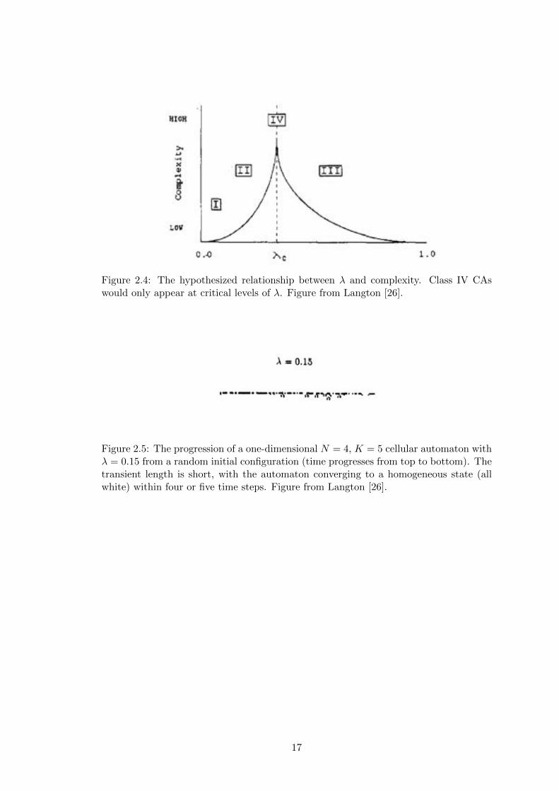
Figure 2.4: The hypothesized relationship between � and complexity. Class IV CAswould only appear at critical levels of �. Figure from Langton [26].
Figure 2.5: The progression of a one-dimensional N = 4, K = 5 cellular automaton with� = 0.15 from a random initial configuration (time progresses from top to bottom). Thetransient length is short, with the automaton converging to a homogeneous state (allwhite) within four or five time steps. Figure from Langton [26].
17
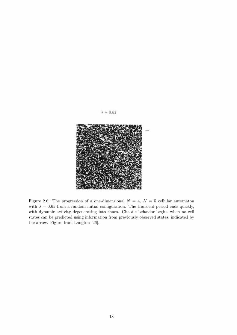
Figure 2.6: The progression of a one-dimensional N = 4, K = 5 cellular automatonwith � = 0.65 from a random initial configuration. The transient period ends quickly,with dynamic activity degenerating into chaos. Chaotic behavior begins when no cellstates can be predicted using information from previously observed states, indicated bythe arrow. Figure from Langton [26].
18
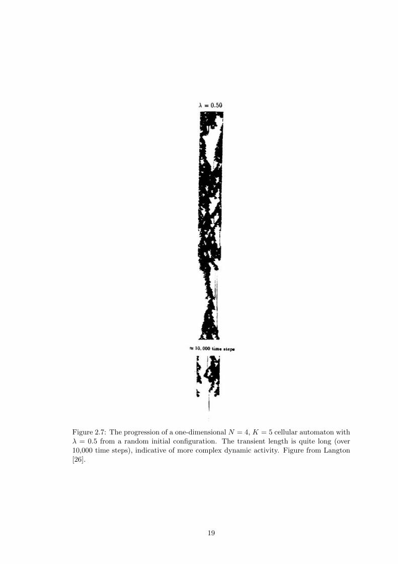
Figure 2.7: The progression of a one-dimensional N = 4, K = 5 cellular automaton with� = 0.5 from a random initial configuration. The transient length is quite long (over10,000 time steps), indicative of more complex dynamic activity. Figure from Langton[26].
19
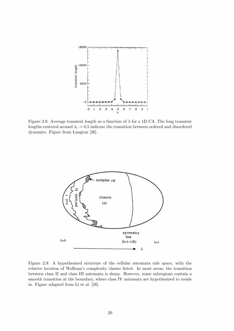
Figure 2.8: Average transient length as a function of � for a 1D CA. The long transientlengths centered around �
c
= 0.5 indicate the transition between ordered and disordereddynamics. Figure from Langton [26].
Figure 2.9: A hypothesized structure of the cellular automata rule space, with therelative location of Wolfram’s complexity classes listed. In most areas, the transitionbetween class II and class III automata is sharp. However, some subregions contain asmooth transition at the boundary, where class IV automata are hypothesized to residein. Figure adapted from Li et al. [28].
20
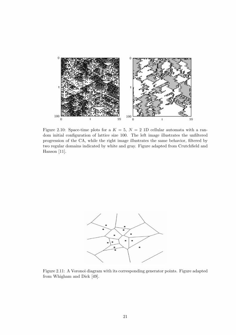
Figure 2.10: Space-time plots for a K = 5, N = 2 1D cellular automata with a ran-dom initial configuration of lattice size 100. The left image illustrates the unfilteredprogression of the CA, while the right image illustrates the same behavior, filtered bytwo regular domains indicated by white and gray. Figure adapted from Crutchfield andHanson [11].
Figure 2.11: A Voronoi diagram with its corresponding generator points. Figure adaptedfrom Whigham and Dick [49].
21
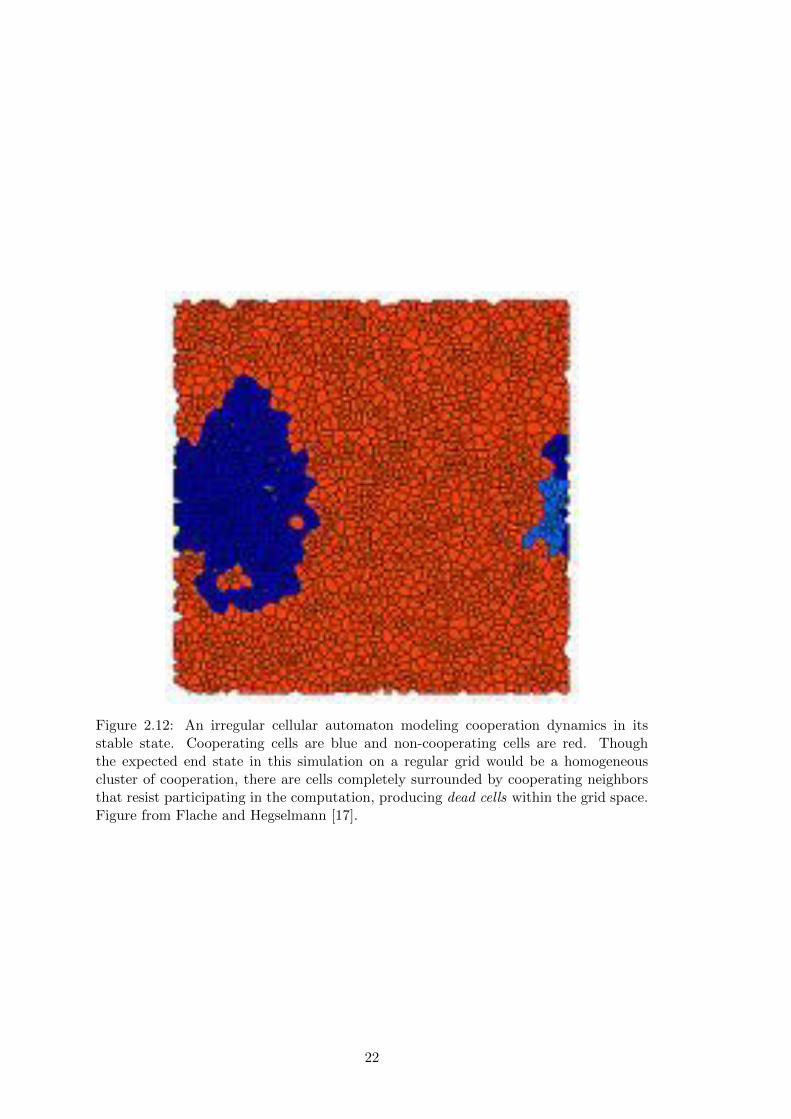
Figure 2.12: An irregular cellular automaton modeling cooperation dynamics in itsstable state. Cooperating cells are blue and non-cooperating cells are red. Thoughthe expected end state in this simulation on a regular grid would be a homogeneouscluster of cooperation, there are cells completely surrounded by cooperating neighborsthat resist participating in the computation, producing dead cells within the grid space.Figure from Flache and Hegselmann [17].
22
Chapter 3
System Design
In this chapter, we will give an overview of the collection of tools we have built and
utilized for our exploration of irregular CA systems. The goal is to provide enough
information so that any experiments described in later chapters can be replicated.
3.1 System Overview
Our CA simulation platform follows an event-driven architecture written in C++; ac-
tions are placed on a queue and are performed one at a time. The event queue structure
allows us to easily interleave actions in between time steps of a CA simulation; for exam-
ple, we can take snapshots of the grid state or dump measurements to a file in between
time steps at any frequency we wish.
We designed this system primarily with flexibility in mind. Modular components
and data structures can easily be swapped in and out of the simulation platform, giving
us fine-grained control over the experiments we are running. Performance is not a
major concern, so long as simulations and experiments can complete within a reasonable
amount of time: for reference an experiment that runs 1,000 simulations 500 time steps
each, writing data to disk at every time step for all simulations takes a few hours in
total to complete.
Termination of the CA simulation occurs either when a maximum time step is
reached, or when a grid state is repeated. We track grid states by walking through
all cells on a grid in a consistent order, appending each cell state to a string array and
then passing the resulting string through a hash function. We keep a history of these
hashes along with the time step they occur, and terminate the simulation if a hash is
ever repeated. Recording the time step also allows us to track the periodicity of any
potential oscillating structures occurring within the simulation.
We execute rule table updates across the grid in a “spreading activation” fashion
in order to increase the performance of the simulator. Instead of visiting and updating
each cell, we track which cells changed state in the previous time step and place those
cells along with their neighbors in a change list. When updating the graph for the next
time step, we only apply the transition rule to cells in the list. We then repeat this
process, updating the list with any cells and their neighbors that have changed state.
23

We initialize the change list at the beginning of the simulation to all cells in the grid.
This method of applying updates allows us to only consider cells that could potentially
change, saving time throughout the CA simulation especially if the grid is large.
3.1.1 Structures
Our CA simulation platform consists of a collection of data structures that are utilized
in tandem to run the simulation. The most essential structures are briefly described
below.
• Grid Generators: The GridGenerator structure stores both the geometric
representation of a grid and the graph representation of a grid. The graph is
implemented as an adjacency list as we expect the graph of a CA grid to be
relatively sparse due to the strictly local connectivity.
• Stencil: A Stencil determines the local neighborhood for each cell in a Grid.
Possible stencils include generalized von Neumann and Moore neighborhoods or
“continuous” stencils that weight neighbors by their distance from the center cell.
• Rule Table: A RuleTable represents a transition rule, utilizing a Stencil to
determine a cell’s neighborhood and compute its next state.
• Geometry Maps: Maps and reverse maps from labels to geometric objects such
as Points, Edges, and Faces are maintained for easy object access and grid
manipulation.
Grid Generators will be reviewed in more detail in Section 3.2, while Stencils and
Rule Tables will be discussed in Section 3.4. A schematic of our overall program archi-
tecture is pictured in Figure 3.1.
3.1.2 Input/Output Files and Running Our System
We have a standardized format for storing and reading in grid configurations, which
allows us to easily pause and restore CA simulations as well as save and transfer them
across di↵erent machines. A representative input grid file can be found in Figure 3.2.
The visual representation of our grids are built by creating graph descriptions for neato,
a graph layout program part of the Graphviz drawing package [16]. Images of our neato
grid representations can be found in Section 3.2. Measured statistics are exported to
.csv files and analyzed using Python with packages from the SciPy ecosystem [25].
We utilize the GNU C library package getopt to pass Unix-style command line
arguments to our system, allowing experiments to be easily scripted and batched across
multiple machines.
3.2 Grid Generation
In this section we will describe the algorithms utilized to generate the various grids.
24
3.2.1 Penrose Tilings
To generate Penrose Tilings and Penrose-connected graphs, we use inflation processes to
recursively generate the tiling. Robinson’s triangle recursive decomposition technique
is utilized to draw both Kite/Dart and Thin/Thick Rhomb tilings, except full tiles are
drawn instead of individual triangles [44]. Though drawing full tiles will likely result
in tiles being considered and drawn multiple times, we avoid this by marking faces as
they are drawn, only keeping a single copy of each face. As in all our grid generation
programs, we track geometric primitives (Point, Edge, Face) to make generating our
standard grid input file straightforward.
3.2.2 Delaunay Triangulations and Voronoi Diagrams
The goal with building grids using Voronoi diagrams is to produce irregular grids that
still respect Euclidean distance, as discussed in Section 2.4.3. Given a set of generator
points {p1, ..., pn} in the plane, a Voronoi polygon Vk
corresponding to a generator
point pk
consists of all points whose distance to pk
is less than its distance to any other
generator point. Thus, we can partition the plane into Voronoi polygons that correspond
to every generator point, producing a Voronoi Diagram. These polygons will serve as
the cells in our CA simulations.
The first step in the process to generate a Voronoi-based grid is to produce generator
points. Though a simple uniform random distribution of points in the plane will generate
a valid Voronoi Diagram, the resulting grid may have undesirable geometric properties
due to the potential for points to clump together. Instead, we can utilize a method
called Poisson Disk Sampling to generate random points that are guaranteed to be at
least some specified distance apart from each other [8]. Points created by this method
will necessarily avoid clumping, illustrated in Figure 3.3.
Once we have a set of generator points, we construct the dual graph of the Voronoi
Diagram, known as the Delaunay Triangulation. The Delaunay Triangulation of a set
of points {p1, ..., pn} in the plane is a triangulation such that no point pk
resides inside
the circumcircle of a triangle; an edge e is considered to be locally Delaunay if the
two triangles that share e as a common edge satisfy the circumcircle condition [13].
We construct this dual graph first because (1) the edges of the Delaunay Triangulation
exactly correspond to the graph connectivity of the Voronoi grid produced by the set
of points and (2) the Voronoi Diagram is easy to construct from the triangulation.
We utilize the Flip Algorithm to construct the Delaunay Triangulation: beginning
with an arbitrary triangulation, edges that are not locally Delaunay are “flipped” such
that they are locally Delaunay. Once there are no more edges to be flipped, then the
resulting triangulation must be a Delaunay Triangulation [14]. Though the flip algorithm
is not the fastest Delaunay Triangulation algorithm, it is straightforward to implement,
requires no auxiliary data structures, and performs well enough for our purposes.
Given a Delaunay Triangulation, we can produce its corresponding Voronoi Diagram
by calculating the circumcenter of each Delaunay triangle and creating an edge between
the circumcenters of adjacent triangles [13, 14]. The circumcenters of the triangles
25

correspond to Voronoi polygon vertices, so we obtain valid Voronoi regions. Thus we
have obtained both the graph representation and the geometric representation of a
Voronoi-based grid. An illustration of this process is shown in Figure 3.4.
3.2.3 Voronoi Quadrilaterals
Experiments and simulations involving � require static neighborhood sizes across all
cells in the grid. One way we address this requirement is by generating irregular grids
that have cells of the same number of sides. Specifically, given a Voronoi Diagram we
can further partition the region such that all cells in the plane are quadrilaterals. This
conversion is accomplished by taking two edge-adjacent Voronoi polygons and forming
a quad from the two generator points and the end points of the shared common edge
between the polygons (Figure 3.5) [41]. As long as the given Voronoi Diagram is well-
formed, specifically with all generator points placed at least some minimum radius from
each other, this quadrilateral generation is possible across an entire Voronoi diagram,
as seen in Figure 3.6. Note that though cells in the resulting VQuad grid always share
edges with four other neighboring cells (excluding the boundary) resulting in uniform
generalized von Neumann neighborhood sizes across the grid, the number of cells they
share vertices with are variable. This variability in vertex adjacency is partially due to
the presence of concave quadrilaterals in the resulting grid.
3.3 Grid Degeneration
In Chapter 6, we consider various degenerated Voronoi Quad grids in our examination
of the � parameter. We will discuss the methods for generating these degraded grids
here.
3.3.1 Generator Point Removal
As noted in Section 3.2.3, VQuad grid generation is dependent on the position of Voronoi
generator points in the input Voronoi diagram. Thus, one manner of grid degeneration
is simply to remove generator points from the input diagram. Since a generator point
in the input diagram could be a vertex to many VQuad cells, generator point removal
has the e↵ect of taking out large chunks of the VQuad grid, as pictured in Figure 3.7.
3.3.2 Crosshatching Degeneration
Though generator point removal provides a simple way to degrade a grid, we wanted
finer-grained control over how points and edges are removed. Thus we devised a man-
ner of degradation that allowed us to specify what local regions of the grid would be
disconnected from other portions of the grid. This basic premise is to draw vertical
and horizontal lines at regular width w intervals apart that subdivide the irregular grid
roughly into square lattice regions. Cell edges that intersect these crosshatchings are re-
moved from the grid with some probability p: cells that were formerly connected by the
26
edge no longer are neighbors in the graph representation of the grid. Thus at p = 1.0 we
would have completely isolated “islands” of grid subregions. This crosshatching degen-
eration technique allows us control over the degree of regional connectivity, as pictured
in Figure 3.8. This manner of degradation preserves the number of cells present in the
grid, instead introducing degradation by decreasing edge adjacency. Though we primar-
ily use crosshatching degeneration as a form of edge removal, this technique also gives us
a way to control generator point removal: since the crosshatchings define a square lattice
partitioning of the grid, we can also choose square regions to remove with some prob-
ability p. Any generator points sitting within the boundary of a chosen square region
will be removed from the graph. Thus we can control both the frequency of generator
points removed (through adjusting p) as well as the average size of the of the regions
removed (through adjusting w). This crosshatching technique allows us to parameterize
the degeneration of a grid beyond simply measuring average neighborhood size.
3.4 Stencil and Rule Table Implementation
3.4.1 Generalized von Neumann and Moore Neighborhoods
We would like to maintain a notion of both von Neumann and Moore neighborhoods even
on irregular grids. Thus we formally define generalized notions of both neighborhood
stencils: a generalized von Neumann neighborhood for a cell c is defined as all cells that
share an edge with c, while a generalized Moore neighborhood for c is defined as all cells
that share a vertex with c. These neighborhood definitions are not necessarily equiv-
alent to their standard definitions. For example, while the generalized von Neumann
neighborhood for Voronoi Quad grids is identical to the regular case, the generalized
Moore neighborhoods are not uniform across the grid and may have neighborhood sizes
ranging from 6 to 12. Because we maintain geometry maps in our system, defining either
neighborhood stencil is straightforward for any CA simulation on any grid.
3.4.2 Game of Life Rule Tables
Conway’s Game of Life (GoL) is a K = 2, N = 9 cellular automaton utilizing a Moore
neighborhood stencil on regular square lattices [19]. Cells are either “alive” or “dead”,
and the rule table has traditionally been described in the following manner:
• Living cells stay alive if 2 or 3 neighbors are alive,
• Living cells with more than 3 living neighbors die from “overcrowding,”
• Living cells with less than 2 living neighbors die from “loneliness,” and
• Dead cells with exactly 3 living neighbors are “born.”
However, we can also describe the GoL rules in terms of a lookup table: since there
are two states, we can map a bit string of length 9 to every possible neighborhood
configuration, with each position in the bit string corresponding a particular cell in the
27

Moore neighborhood stencil (Figure 3.9). This manner of encoding allows us to quantify
and manipulate a CA’s rule table, and we utilize this representation when conducting �
experiments as described in the next section.
3.4.3 � Rule Tables
In the � experiments performed by Wootters and Langton, rule tables must be isotropic:
all planar rotations of a particular neighborhood configuration map to the same out-
put cell state. This condition removes the global property of spatial orientation from
influencing rule transitions [4, 52]. As a result, what would be a KN sized table results
in a smaller table because only rotationally distinct neighborhood configurations are
unique entries: specifically, if we consider the K = 8, N = 5 case the rule table of size
85 = 32, 768 is reduced to a rule table of size 8, 352 (see Appendix B.1 for calculation).
To generate these tables, we iterate over all KN possible neighborhood values, canon-
icalize their string representations by finding their lexicographically minimal rotation,
and track only the unique neighborhoods. For example, in the K = 8, N = 5 case,
neighborhoods “0110” and “1001” map to the same minimal rotation neighborhood of
“0011”. We then append a center state value to the end of this canonical neighborhood
representation, thus creating the keys for our � rule table mapping with the output state
for that particular neighborhood configuration as the value.
Rule tables must also be strongly quiescent in that a neighborhood configuration that
consists entirely of the quiescent state must map to the quiescent state. This condition
is satisfied by simply initializing the appropriate entry in the transition table and then
ensuring that entry is not modified throughout a given experiment run.
3.5 Summary
We have built a CA simulation system that is modular and extensible. Our system
performs su�ciently well to run a gamut of CA experiments within a reasonable amount
of time. The system is also flexible enough so that we can make changes to any portion
of the system through implementing various derived classes, and the command line
interface allows us to easily tweak experiment parameters without having to change the
source code.
28
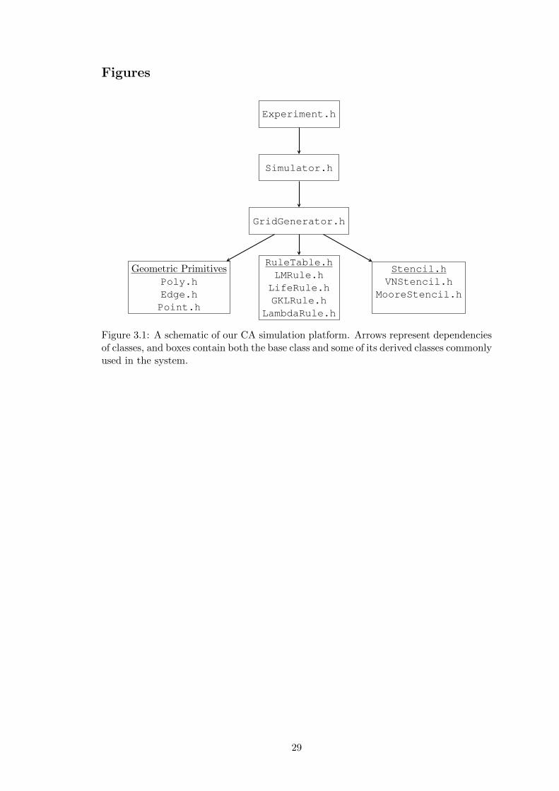
Figures
Experiment.h
Simulator.h
GridGenerator.h
RuleTable.h
LMRule.h
LifeRule.h
GKLRule.h
LambdaRule.h
Stencil.h
VNStencil.h
MooreStencil.h
Geometric PrimitivesPoly.h
Edge.h
Point.h
Figure 3.1: A schematic of our CA simulation platform. Arrows represent dependenciesof classes, and boxes contain both the base class and some of its derived classes commonlyused in the system.
29
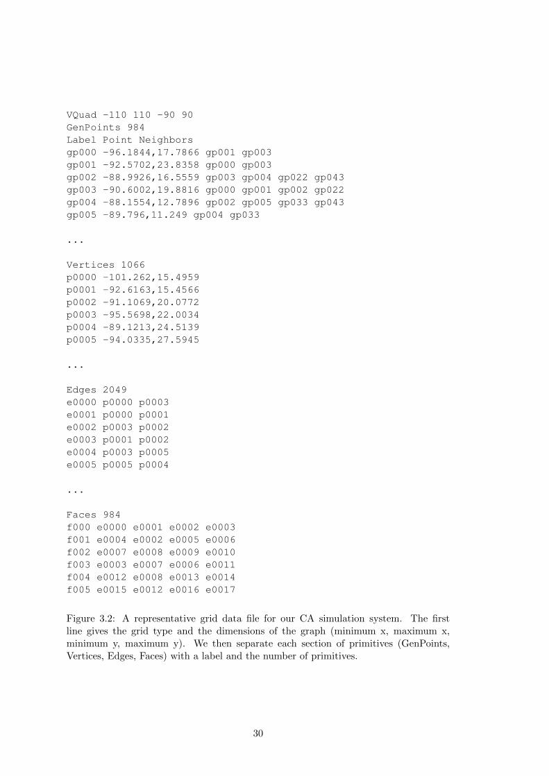
VQuad -110 110 -90 90
GenPoints 984
Label Point Neighbors
gp000 -96.1844,17.7866 gp001 gp003
gp001 -92.5702,23.8358 gp000 gp003
gp002 -88.9926,16.5559 gp003 gp004 gp022 gp043
gp003 -90.6002,19.8816 gp000 gp001 gp002 gp022
gp004 -88.1554,12.7896 gp002 gp005 gp033 gp043
gp005 -89.796,11.249 gp004 gp033
...
Vertices 1066
p0000 -101.262,15.4959
p0001 -92.6163,15.4566
p0002 -91.1069,20.0772
p0003 -95.5698,22.0034
p0004 -89.1213,24.5139
p0005 -94.0335,27.5945
...
Edges 2049
e0000 p0000 p0003
e0001 p0000 p0001
e0002 p0003 p0002
e0003 p0001 p0002
e0004 p0003 p0005
e0005 p0005 p0004
...
Faces 984
f000 e0000 e0001 e0002 e0003
f001 e0004 e0002 e0005 e0006
f002 e0007 e0008 e0009 e0010
f003 e0003 e0007 e0006 e0011
f004 e0012 e0008 e0013 e0014
f005 e0015 e0012 e0016 e0017
Figure 3.2: A representative grid data file for our CA simulation system. The firstline gives the grid type and the dimensions of the graph (minimum x, maximum x,minimum y, maximum y). We then separate each section of primitives (GenPoints,Vertices, Edges, Faces) with a label and the number of primitives.
30
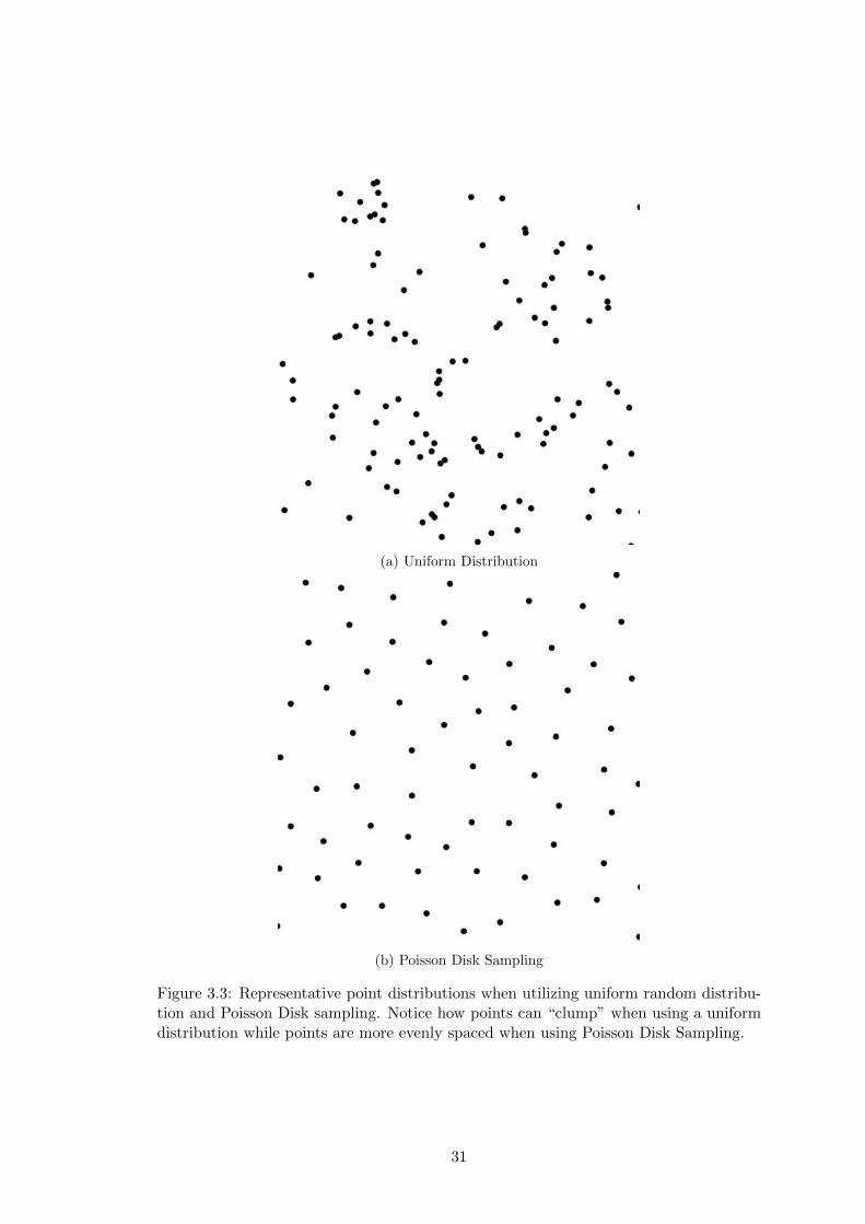
(a) Uniform Distribution
(b) Poisson Disk Sampling
Figure 3.3: Representative point distributions when utilizing uniform random distribu-tion and Poisson Disk sampling. Notice how points can “clump” when using a uniformdistribution while points are more evenly spaced when using Poisson Disk Sampling.
31
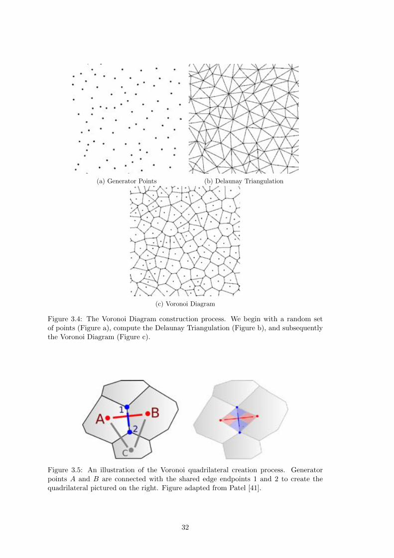
(a) Generator Points (b) Delaunay Triangulation
(c) Voronoi Diagram
Figure 3.4: The Voronoi Diagram construction process. We begin with a random setof points (Figure a), compute the Delaunay Triangulation (Figure b), and subsequentlythe Voronoi Diagram (Figure c).
Figure 3.5: An illustration of the Voronoi quadrilateral creation process. Generatorpoints A and B are connected with the shared edge endpoints 1 and 2 to create thequadrilateral pictured on the right. Figure adapted from Patel [41].
32
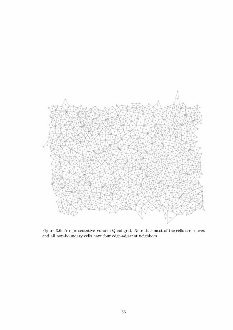
Figure 3.6: A representative Voronoi Quad grid. Note that most of the cells are convexand all non-boundary cells have four edge-adjacent neighbors.
33

Figure 3.7: A VQuad grid degraded by the removal of 7% of the input generator points.Notice the lack of small, (particularly single cell) holes in the resulting grid.
34

Figure 3.8: An illustration of a p = 1.0, w = 20 crosshatch degenerated grid: edgesmarked in red have been removed from the connectivity graph.
Neighborhood Output000000111 1110001101 0000010001 0001010100 1
Figure 3.9: A few representative entries in the Game of Life Rule Table (there are 29
entries in total). The center cell is the rightmost bit, in bold. These table entriescorrespond exactly to the four Game of Life rules as described in Chapter 3.4.2.
35
Chapter 4
Penrose Life Experiments
We begin our exploration of irregular CA by considering aperiodic tilings. Specifically,
we build upon work done by Hill et al. (see Chapter 2.4.2) in examining the Game of Life
on Penrose Tilings (Penrose Life). Aperiodicity is a move away from the regularity found
in square lattices but still maintains some local neighborhood structure. One of our goals
is to investigate the potential for information transfer across an irregular CA space. In
the case of Game of Life, moving particles called gliders are the most basic representation
of information transfer across a regular grid. However, these gliders exploit the regularity
of the grid in their movement and as a result are not robust to changes in their immediate
environment: over 99% of possible environment configurations a glider can encounter
will be destructive to it [6]. Thus we imagine that information transfer may be more
di�cult to achieve on grids that do not maintain spatial consistency. These Penrose Life
investigations explore the possibility of moving particles in a CA grid that relaxes some
of the regularity found in standard square lattices.
Another goal is to investigate CA behavior at the boundary of the grid. Typical CA
simulations assume toroidal boundaries that produce an “infinite” grid wrapping around
on itself, but natural dynamic systems are unlikely to have this property. Finite spaces
will inevitably have boundaries and complex CA must be able to handle these unique
conditions where the neighborhood for a cell on the boundary is incomplete. Since
toroidal boundary conditions are impossible for an aperiodic tiling, we will examine
potential boundary interactions in Penrose Life.
Hill et al. ran experiments on Kite/Dart Penrose tilings investigating random initial
starting configurations (soups) and the resulting stable structures left on the grid (ash).
Owens and Stepney continued this work on Thin/Thick Rhombus Penrose tilings and
also examined repeating periodic structures (oscillators) in Penrose Life. We replicate
and extend their work here as well.
4.1 Lifetime to Stability and Ash Density
In order to locate where interesting behavior may occur in Penrose Life, we begin by
examining the full range of initial soup densities (percentage of ON cells in the starting
configuration) from d = 0.01 to d = 0.99, measuring both lifetime to stability (the
36

number of timesteps a given configuration takes to stabilize) and final ash density (the
percentage of the grid in a stable state).
Experimental Setup
Both Kite/Dart and Thin/Thick Rhomb Penrose tilings are considered. We utilize
circular grids, with the Kite/Dart grid containing 995 cells and Rhomb grid containing
1,075 cells. The Rule Table utilizes standard Game of Life rules with generalized Moore
neighborhood stencils. For each initial soup density we run 100 trials and average our
statistics across all the trials, resulting in 9,900 total CA simulations. The tilings are
pictured in Figure 4.1.
Results
Lifetime to Stability and Ash Density graphs for Kites/Darts are pictured in Figure 4.2.
These results agree with the data presented by Hill et al. shown in Figure 4.3, with
our circular tiling falling in between the S and M grids in terms of size: both lifetime
graphs have a right-skewed distribution while the ash density plots show little correlation
between lifetime and final ash density for initial soup densities of d = 0.20, 0.40, 0.60.
The ash densities fall within a range of about d = 0.00 to d = 0.03. It is important to
note that though the lifetime graphs have the same distribution shape as the standard
Game of Life lifetime graph, the average lifetimes for the Penrose tilings are much lower
than the standard grid (Figure 4.4a). Similarly, though the ash density plots for the
standard grid show no correlation between lifetime and ash density like the Kite/Dart
plot (Figure 4.4b), the final ash densities fall in a higher range of about d = 0.02 to
d = 0.06. These results suggests that the overall qualitative behavior of Penrose Life
could be similar to the standard Game of Life but also shows that it is much more
di�cult to maintain coherent Life structures on irregular grids.
We also collected data for Lifetime to Stability and Ash Density graphs for Rhombs as
shown in Figure 4.5. The lifetime graph for the Rhomb tiling possesses the same overall
right-skewed shape as all the other lifetime graphs we have examined, and outside of
a few outliers the ash density plot shows no correlation between lifetime and final ash
density either. Again, the final ash densities fall within a range of d = 0 to d = 0.03
like the Kite/Dart tilings. However, the overall average lifetime for the Rhomb tiling is
greater than the lifetimes for the Kite/Dart tiling (Figure 4.6); we speculate that this is
due to the convexity of the Rhomb tiles which allow for larger neighborhood sizes which
then allow more opportunities for ON cells to proliferate. We will examine neighborhood
di↵erences in more detail in Section 4.3.
4.2 Single Run Analysis
The longest run we observed in our Kite/Dart simulations began with an initial soup
density of d = 0.22 and had an active lifetime of 173 timesteps before periodic behavior
set in. We graph the active density of ON cells in the tiling against time in Figure 4.7.
37
As seen in this graph, the active density of the Penrose quickly falls to near typical
ash density levels (d ⇡ 0.03) and stays close to constant over a majority of its life-
time. We hypothesize that this behavior would be indicative of ash stabilizing relatively
quickly with a small glider-like structure being primarily responsible for the long life-
time. Looking at the actual simulation, this seems to be the case, with an amorphous
moving structure propagating in the upper left corner for majority of the simulation.
Otherwise, the ash is largely settled, with a plinker (coined by Hill et al.), a period 2
oscillator, present on the right side of the tiling.
The longest run observed in our Rhomb simulations began with an initial soup
density of d = 0.26 had an active lifetime of 666 timesteps. Its density is plotted against
time in Figure 4.9. Unlike the Kite/Dart single run, there are some fluctuations in the
active density of ON cells in the grid throughout the run. Upon visual inspection of
the run (seen in Figure 4.8), there is spreading activation across the grid when moving
structures collide with stable structures or oscillators, resulting in the spikes in density
such as the one beginning around timestep 200.
In either run, the most coherent structures are oscillators; “glider-like” objects strug-
gle to emerge and move across the grid, with most movement occurring haphazardly
across the tilings with no well-defined direction or structural boundaries like standard
Game of Life gliders. This was expected due to the aperiodic nature of Penrose tilings,
with structural coherency only possible within localized regions of the tiling as neigh-
borhood size and structure will vary across the grid. With the experiments and data
collected thus far, it appears that e↵ective information transfer will be di�cult to achieve
within Penrose Life of either tiling.
4.3 Neighborhood Analysis
We see a significant di↵erence between the average lifetimes of the Kite/Dart and Rhomb
tilings, primarily due to di↵ering local neighborhood characteristics. The possible neigh-
borhood configurations for both tilings are pictured in Figure 4.10. We see that Rhomb
tilings have many stencil configurations with a neighborhood size of ten or greater,
while the Kite/Dart tilings only have one such stencil configuration. This is likely to
give Rhomb tilings higher average neighborhood sizes across an entire tiling. Neigh-
borhood size frequencies for our circular tilings are pictured in Figure 4.11. The most
frequent neighborhood size for our Kite/Dart tiling is 9, whereas the most frequent
neighborhood size for our Rhomb tiling is 10. The average neighborhood size is indeed
higher for Rhombs than it is for Kite/Darts, as shown in Table 4.13. This data suggests
that increased connectivity would allow for longer lifetimes, as there would be more
opportunities for birth. Also note that both tilings have a higher neighborhood size
than regular square grids, which have a neighborhood size of 8. Thus we cannot solely
rely on connectivity when evaluating a grid’s ability to support Life or other complex
behavior.
Because tiles on the boundary have incomplete neighborhoods, we may get di↵ering
38
behavior at the border of the tiling that may impact lifetime or ash density. To inves-
tigate potential impact of border tiles, we recorded the neighborhood frequency for the
Rhomb single run discussed in Section 4.2, pictured in Figure 4.12. Neighborhood sizes
of 6 or less only occur at the boundaries, making them incomplete neighborhoods for the
Rhomb tiling. Since we do see some activity throughout the lifetime of the simulation
at these border cells, we need to consider ways to examine boundary e↵ects. One option
we explore in the following section is to place an initial starting configuration within a
subregion of a larger graph and then only consider activity in the subregion.
4.4 Subregion Analysis
As shown by Hill et al. in Figure 4.3, the size of the grid impacts the average lifetime.
In order to investigate both border and size e↵ects on the lifetime of Penrose Life, we
ran subregion experiments. The purpose of these experiments is to explore Penrose Life
behavior without the e↵ect of a boundary: the subregions are chosen such that boundary
interactions are not measured.
Experimental Setup
We generated much larger circular Kite/Dart (6484 tiles) and Rhomb (7007 tiles) tilings,
but only initialized a subregion of the tiling (Figure 4.14). The subregion radius is chosen
to match the smaller grid we have previously analyzed as close as possible with the idea
of replicating the original starting configurations of our first set of lifetime experiments
but providing more grid space and removing boundary cell e↵ects. Lifetime to Stability
and Ash Density are calculated in the same manner with the same number of trials as
before, with 100 di↵erent initial configurations for each initial soup density from d = 0.01
to d = 0.99 giving 9900 total trials. Ash density is only measured within the subregion.
Results
The Lifetime to Stability graph comparing our initial Kite/Dart tiling to the larger
subregioned tiling is shown in Figure 4.15a. There is not a significant increase in life-
time at the peak initial soup densities, though the larger grid appears to have less of a
fall-o↵ of average lifetime at higher initial densities. The analogous graph for Rhomb
tilings is shown in Figure 4.15b. For Rhombs, we do see a large increase in lifetimes
across all densities. The di↵erences between Kite/Darts and Rhombs in average life-
times for large tilings could be due to the relative increased connectivity of the large
Rhomb tilings when there are no boundaries present: if we take the weighted average
of incomplete neighborhood sizes for both Kite/Darts and Rhombs as shown in Fig-
ure 4.11, the Kite/Dart average incomplete neighborhood size (6.27) is higher than the
Rhomb incomplete neighborhood size (5.12). Coupled with the fact Rhomb tilings have
a larger average neighborhood size (Figure 4.13), the “removal” of boundaries from the
subregioned tilings would produce a more dramatic change in neighborhood sizes for
39

the Rhomb tiling in comparison to the Kite/Dart tiling. This di↵erence could also po-
tentially be due to other factors, such as the geometric or spatial orientation of the two
di↵erent types of Penrose tilings.
Ash density scatter plots for our subregion Kite/Dart and Rhomb tilings are pictured
in Figure 4.16a and Figure 4.16b. Note that the ash density values are only measured
within the subregion of initialization; ash in the outer regions of the tiling are not
included in the density calculation. We see again that there is no correlation between
lifetime and ash density as shown by both plots, and the ash densities fall roughly the
same ranges we have seen before. In Figure 4.16b there are a number of simulations
that have a final ash density of zero for Rhomb tilings. This could be due to moving
structures that travel outside the subregion, which makes sense as the average lifetime for
Rhomb tilings is also much higher than the average lifetime for Kite/Dart tilings. These
subregion experiments illustrate that Rhomb tilings may have fundamental properties
di↵erent from the Kite/Dart tilings beyond neighborhood size that allow for long-lived
Penrose Life runs.
4.5 Potential for Penrose Gliders
With the ash density results shown for subregion Rhomb tilings along with the signifi-
cantly higher average lifetime for Rhomb tilings in general, there is some potential for
gliders to be found in Penrose Rhomb Life. Unfortunately, like Owens and Stepney who
also searched for gliders in Penrose tilings [39], the only coherent structures we have de-
tected in either tiling are oscillators. It appears that the aperiodic nature of the Penrose
tilings severely limits the ability for coherent structures to travel beyond a particular
localized region within Penrose Life.
However, if we move away from the Game of Life rules, there is potential for coher-
ent moving structures to exist on Penrose tilings. Goucher created a 4-state CA rule
table that supports a coherent glider structure on both Kite/Dart and Rhomb tilings
(Figure 4.17) [20]. This discovery illustrates that aperiodicity does not completely limit
the ability for a CA to transfer information across a grid space; in fact it has been
conjectured that a CA rule table can be created for any quadrilateral tiling, provided
that the automaton has enough possible states [35].
Another possibility is the we might be able to support, at a higher granularity, a
regular grid composed of cells from an irregular grid. For example, notice that a par-
ticular orientation of a Rhomb tiling could induce a “regular” grid. Perhaps these cells
can coordinate activity at an intermediate structural level, producing mosaic behavior
as observed by Messinger et al. [30]. The Local Isomorphism Theorem [15] suggests that
the number of possible configurations is bounded and thus manageable by such a system
attempting to coordinate at a meso-scale. Thus, at this level, gliders on Penrose tilings
could be programmed in a more traditional way. This work suggests that support of a
larger grid may require neighborhood-specific approaches.
40
4.6 Summary
We have conducted various tests examining the behavior of the Game of Life on aperiodic
Penrose tilings. By replicating and extending the work of Hill et al. to both Kite/Dart
and Rhomb tilings, we have shown that though Penrose Life has some similar qualitative
properties to the standard Game of Life, there are significant di↵erences in terms of
lifetime and ash density between the two CAs. We see that the aperiodicity of the
Penrose tilings hampers the ability for information transfer to occur across the grid as
the only coherent structures we have detected in our simulations are oscillators.
Additionally, there appear to be some quantitative di↵erences between the Kite/Dart
and Rhomb tiling’s ability to support Penrose Life as evidenced by the much higher av-
erage lifetimes of simulations on the Rhomb tilings. Possible sources of these di↵erences
could be the higher average neighborhood size or the geometric properties (such as con-
vexity) of the Rhomb tilings. Boundary conditions and overall grid size also appear to
impact a grid’s ability to support complex CA behavior. These attributes of irregular
grids will be examined further in the following chapters.
41
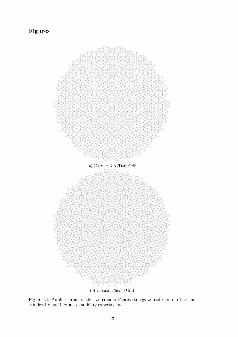
Figures
(a) Circular Kite/Dart Grid
(b) Circular Rhomb Grid
Figure 4.1: An illustration of the two circular Penrose tilings we utilize in our baselineash density and lifetime to stability experiments.
42

(a) Kite/Dart Lifetime to Stability Graph
(b) Kite/Dart Ash Density Scatter Plot
Figure 4.2: Lifetime to Stability and Ash Density graphs for the Kite/Dart circulartiling, grid size = 995. We see the same right-skewed distribution for lifetimes as seenin Hill et al.’s results. There appears to be no correlation between final ash density andthe lifetime of simulation.
43
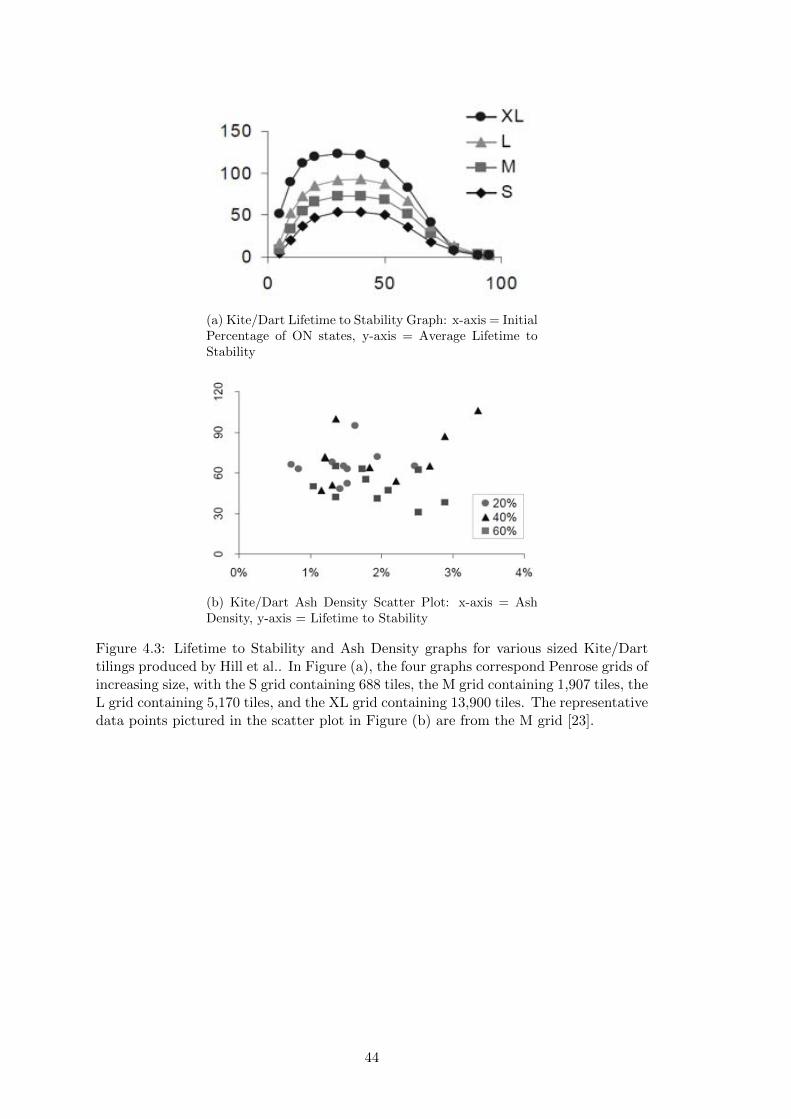
(a) Kite/Dart Lifetime to Stability Graph: x-axis = InitialPercentage of ON states, y-axis = Average Lifetime toStability
(b) Kite/Dart Ash Density Scatter Plot: x-axis = AshDensity, y-axis = Lifetime to Stability
Figure 4.3: Lifetime to Stability and Ash Density graphs for various sized Kite/Darttilings produced by Hill et al.. In Figure (a), the four graphs correspond Penrose grids ofincreasing size, with the S grid containing 688 tiles, the M grid containing 1,907 tiles, theL grid containing 5,170 tiles, and the XL grid containing 13,900 tiles. The representativedata points pictured in the scatter plot in Figure (b) are from the M grid [23].
44

(a) Standard GoL Lifetime to Stability Graph: x-axis =Initial Percentage of ON states, y-axis = Average Lifetimeto Stability
(b) Standard GoL Ash Density Scatter Plot: x-axis = AshDensity, y-axis = Lifetime to Stability
Figure 4.4: The Lifetime to Stability graph for standard grids produced by Hill et al..The grid sizes were chosen to be as close as possible to their Penrose counterparts, withthe S grid containing 676 cells, the M grid containing 1,937 cells, the L grid containing5,184 cells, and the XL grid containing 13,924 cells. The data points pictured in Figure(b) are from the M grid [23].
45

(a) Rhomb Lifetime to Stability Graph
(b) Rhomb Ash Density Plot
Figure 4.5: Lifetime to Stability and Ash Density graphs for the Rhomb circular tiling,grid size = 1,075. The same overall lifetime distribution shape is seen in the Rhombcase, albeit with more fluctuation especially from initial ON percentage values from 20to 60. The ash density scatter plot again shows no correlation between final density andlifetime.
46

Figure 4.6: Lifetime graphs for both our circular Kite/Dart and Rhomb tilings. Notethe same overall right-skewed distribution for both graphs and the significantly higheraverage lifetime of Rhomb simulations.
Figure 4.7: Active density plotted against time for an initial soup density of d = 0.22on our circular Kite/Dart tiling. The lifetime of the run was 173 timesteps, with a finalash density of d = 0.0190. We see a steep drop-o↵ of active density until it stabilizesaround time step 60. The low but relatively constant active density could be due to aglider-like structure moving within the grid.
47

‘’(a) t=190
(b) t=191
(c) t=192 (d) t=193
(e) t=194 (f) t=195
48
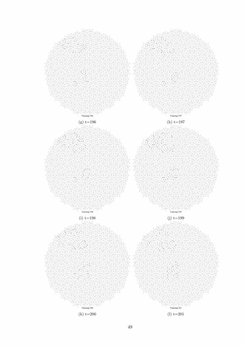
(g) t=196 (h) t=197
(i) t=198 (j) t=199
(k) t=200 (l) t=201
49

(m) t=202 (n) t=203
(o) t=204 (p) t=205
Figure 4.8: Timesteps 190-205 of the Rhomb single run sequence with initial densityd = 0.26. Note the sudden proliferation of ON states in the upper left when the movingstructure collides and interacts with the border. This spike in activity can be seen inthe corresponding lifetime graph (Figure 4.9).
50
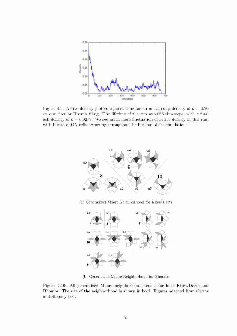
Figure 4.9: Active density plotted against time for an initial soup density of d = 0.26on our circular Rhomb tiling. The lifetime of the run was 666 timesteps, with a finalash density of d = 0.0279. We see much more fluctuation of active density in this run,with bursts of ON cells occurring throughout the lifetime of the simulation.
(a) Generalized Moore Neighborhood for Kites/Darts
(b) Generalized Moore Neighborhood for Rhombs
Figure 4.10: All generalized Moore neighborhood stencils for both Kites/Darts andRhombs. The size of the neighborhood is shown in bold. Figures adapted from Owensand Stepney [38].
51
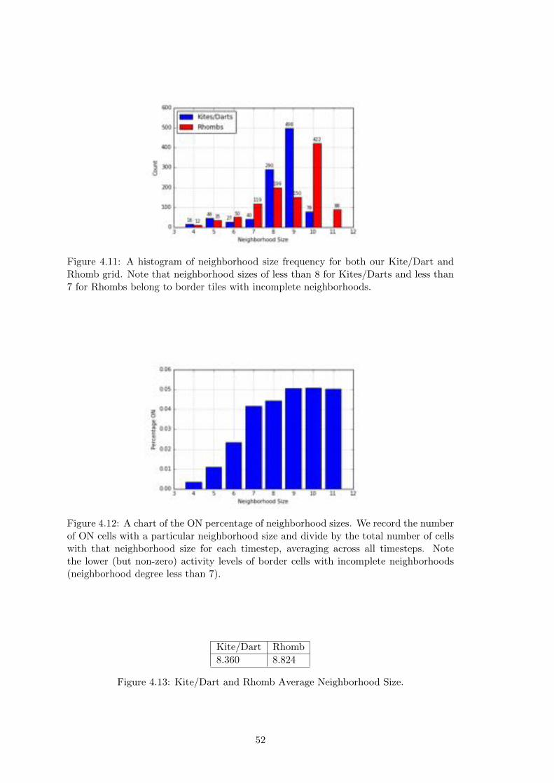
Figure 4.11: A histogram of neighborhood size frequency for both our Kite/Dart andRhomb grid. Note that neighborhood sizes of less than 8 for Kites/Darts and less than7 for Rhombs belong to border tiles with incomplete neighborhoods.
Figure 4.12: A chart of the ON percentage of neighborhood sizes. We record the numberof ON cells with a particular neighborhood size and divide by the total number of cellswith that neighborhood size for each timestep, averaging across all timesteps. Notethe lower (but non-zero) activity levels of border cells with incomplete neighborhoods(neighborhood degree less than 7).
Kite/Dart Rhomb8.360 8.824
Figure 4.13: Kite/Dart and Rhomb Average Neighborhood Size.
52

Figure 4.14: An illustration of subregion initialization for our large Kite/Dart tiling(6484 tiles). The initial soup density within the subregion is d = 0.09.
53
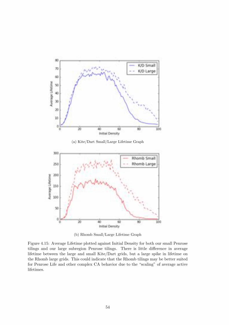
(a) Kite/Dart Small/Large Lifetime Graph
(b) Rhomb Small/Large Lifetime Graph
Figure 4.15: Average Lifetime plotted against Initial Density for both our small Penrosetilings and our large subregion Penrose tilings. There is little di↵erence in averagelifetime between the large and small Kite/Dart grids, but a large spike in lifetime onthe Rhomb large grids. This could indicate that the Rhomb tilings may be better suitedfor Penrose Life and other complex CA behavior due to the “scaling” of average activelifetimes.
54
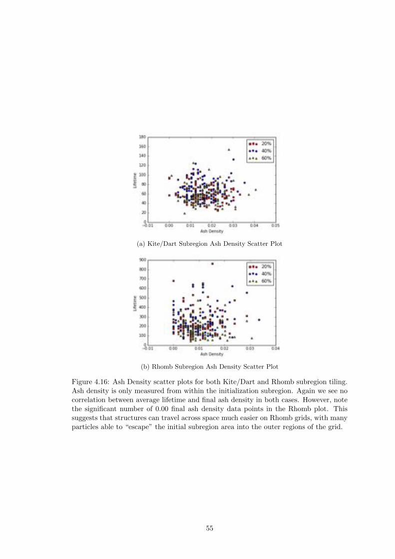
(a) Kite/Dart Subregion Ash Density Scatter Plot
(b) Rhomb Subregion Ash Density Scatter Plot
Figure 4.16: Ash Density scatter plots for both Kite/Dart and Rhomb subregion tiling.Ash density is only measured from within the initialization subregion. Again we see nocorrelation between average lifetime and final ash density in both cases. However, notethe significant number of 0.00 final ash density data points in the Rhomb plot. Thissuggests that structures can travel across space much easier on Rhomb grids, with manyparticles able to “escape” the initial subregion area into the outer regions of the grid.
55

Figure 4.17: An illustration of the path of the Penrose glider discovered by Goucher. It isa 4-state cellular automaton which produces structures that can travel along “ribbons”of rhombi without ever looping back to its original location. Figure from Goucher [20].
56
Chapter 5
Local Majority Experiments
As discussed in Chapter 2.3, Messinger et al. investigated CA performance on the major-
ity task in the presence of various irregularities, such as temporal state noise, nonuniform
rule tables and random connectivity in an exploration of robustness in stomatal dynamic
systems. We extend this work by examining the e↵ects of spatial irregularity on CA
majority task performance.
5.1 Baseline Majority Task Performance on Irregular Grids
Our extensions of majority task experiments will focus on the local majority rule table
for 2-state cellular automata. The rules are simple:
• If there is a majority of ON or OFF cells in a cell c’s neighborhood, then c will
transition to the majority state, and
• If there is no majority, c will retain its previous state.
This rule table represents the most basic manner of solving the majority task and is
easily extended to grids with variable neighborhood sizes.
Experimental Setup
We mirror Messinger et al.’s experimental setup in order to compare our results with
theirs. For regular grids, a 15 by 15 grid (225 total cells) is utilized with periodic
boundaries. We begin with a 1:99 ON:OFF ratio, incrementing by 1 up to 99:1. The
simulation is run for a maximum of 450 time steps, recording only completely correct
classification. 1,000 random grid configurations are used for every starting ratio, giving
a total of 99,000 trials. A single complete run of all the trials takes approximately 25
minutes in our simulation system.
We use Delaunay and Voronoi generation methods to generate our irregular grids.
Our experiments utilize both a grid created through Poisson Disk generator points (Fig-
ure 5.1) as well as a grid derived from a plant stomatal array. For the stomatal array, we
begin with an image of the stomata and drop points where the stoma are located. We
57

then utilize these points as generator points for a Delaunay triangulation. The entire
process is pictured in Figure 5.2.
Results
First we replicated Messinger et al.’s baseline experiments to confirm the accuracy of
our system, with our results corresponding exactly with theirs (Figure 5.3). The general
profile of the Local Majority Task performance curve is symmetric, with a severe fall-o↵
in task performance at around ON:OFF ratios of 15:85 and 85:15 and 0% task perfor-
mance between ratios of about 30:70 to 70:30. Since the majority classification tasks
become increasingly di�cult as the ON:OFF ratio approaches 50:50, this degradation
in performance is to be expected for such a simple rule. For comparison, the task per-
formance of a more complex rule table created through the use of a genetic algorithm is
also pictured in Figure 5.3a. The overall performance of this rule table is much better
than the local majority rule, but also sees a drop in performance when classifying 50:50
initial ratios.
The task performance of our two irregular grids are pictured in Figure 5.4. We
see that both irregular grids have the same symmetric task performance profile as the
baseline regular grids. This result suggests that irregular grids could be suitable for
supporting complex behavior comparable to regular grids. It is also important to note
that both irregular grids lack periodic boundary conditions unlike the baseline regular
case. The absence of periodicity decreases neighborhood connectivity and will hurt a
CA’s ability to transfer information across the grid space, making the task performance
of the irregular grids even more remarkable. For comparison, local majority task perfor-
mance for regular grid is reduced significantly when periodic boundary conditions are
removed, shown in Figure 5.5. Thus, it appears that in the context of the majority task,
spatial irregularity will not hinder the performance or behavior of a CA system. The
fact that local majority task performance is essentially equivalent across both square
and spatially irregular grids establishes a rough form of equivalence between the two
grid types within the domain of the CA majority task.
5.2 Majority Task Performance with State Noise
Messinger et al. discovered in their investigations that introducing small amounts of
state noise improves the performance of majority task CA, likely due to the fact that the
random state change will stimulate movement across the grid [30]. We will investigate
the impact of state noise in more detail and in the context of irregular grids.
Experimental Setup
Data for task performance graphs is collected with the same setup and number of trials as
in the previous section. State noise is introduced by changing each cell’s correct output
state with probability ⌘ before the next timestep. State noise is not applied if the CA
has reached a uniform configuration of either all ON or all OFF states. Since Messinger
58
et al. reported that state noise probabilities of ⌘ � 0.1 caused massive degradation of
majority task performance, we consider a range of state noise from ⌘ = 0.01 to ⌘ = 0.15.
Since initial ON:OFF ratios near 50:50 are the most di�cult starting configurations
to classify, we also perform experiments that measure the impact of state noise on “hard”
initial configurations. For each state noise percentage, we generate 1,000 random initial
configurations with ON:OFF ratios chosen from a Gaussian distribution N (0.5, 0.06).
Results
Task performance graphs for regular grids with state noise ⌘ = 0.05 and ⌘ = 0.15 are
shown in Figure 5.6. We see that with an introduction of a small amount of noise
(⌘ = 0.05) task performance dramatically improves, with incorrect classifications only
occurring between ON:OFF ratios of 40:60 and 60:40 and with roughly 35% correct
classifications of 50:50 starting ratios. Conversely, when too much noise is introduced to
the system (⌘ = 0.15), task performance across all starting ratios degrade below baseline
levels. The task performance graphs for the irregular stoma grid with ⌘ = 0.05, 0.15
also exhibit the same trend (Figure 5.7). However, for the stoma grid with ⌘ = 0.05
only about 10% of the 50:50 starting ratios are correctly classified, which is poorer
performance on 50:50 configurations compared to the regular grid. Overall however, the
regular and irregular grids exhibit the same sort of behavior when varying levels of state
noise are applied. With the addition of small amounts of state noise, the basic Local
Majority rule table performs similarly to more complex rule tables; the performance
graph for both regular and irregular grids at ⌘ = 0.05 closely resembles the performance
graph of the Sip rule pictured in Figure 5.3a, one of the best performing rule tables
evaluated by Messinger et al. [30].
The results for local majority task performance on “hard” configurations on both
regular and stoma grids are shown in Figure 5.8. We see that task performance sig-
nificantly increases when state noise ⌘ � 0.02 and then quickly degrades when state
noise ⌘ � 0.12 for both grids. In the regular case, task performance stays relatively
steady just above 70% when 0.02 ⌘ 0.12 while in the irregular stomatal case task
performance gradually rises to about 60% correct classification in that same state noise
range. These results confirm that small amounts of state noise is beneficial for majority
task performance, regardless of the spatial dynamics of the grid. These results also con-
firm the viability of irregular Voronoi grids in supporting majority task behavior, with
task performance on the stomatal grid closely resembling the results on regular grids
throughout all these experiments.
5.3 Summary
We have evaluated local majority task performance on both regular grids and irregular
Voronoi grids. The profiles of the performance graphs show remarkable similarities
between the regular and irregular grids in majority task performance. These similarities
continue when we examine the impact of state noise, though the irregular grids perform
59
slightly worse than the regular grids when noise is introduced. Still, we see that small
amounts of state noise improve task performance in both the regular and irregular
grid cases, with their overall classification percentages rivaling those of more complex,
human-engineered majority task rule tables.
Thus, we see more evidence that randomness can facilitate the function of decen-
tralized dynamic systems, and it seems plausible that biological systems utilizing local
communication can overcome spatial irregularity and perform comparably to “perfect”
CA systems even in noisy environments. Again, we see some evidence that spatially ir-
regular grids can be functionally equivalent to their regular counterparts within a specific
CA task domain.
60

Figures
Figure 5.1: The Delaunay Triangulation (and thus connectivity graph) for our generatedirregular grid. Dimensions for the Poisson Disk sampling were chosen so that the cellcount would match the 15 by 15 size of the baseline regular grid as close as possible.
61

(a) Original Stomatal Array Image
(b) Stomatal Array with Stomata Marked
(c) Stomatal Delaunay Triangulation
Figure 5.2: An illustration of the process we use to generate a grid from a stomatal arrayimage. The final grid pictured is the Delaunay Triangulation of the generator points,which corresponds to the connectivity graph we utilize for the majority task CA.
62
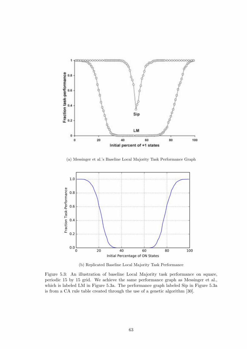
(a) Messinger et al.’s Baseline Local Majority Task Performance Graph
(b) Replicated Baseline Local Majority Task Performance
Figure 5.3: An illustration of baseline Local Majority task performance on square,periodic 15 by 15 grid. We achieve the same performance graph as Messinger et al.,which is labeled LM in Figure 5.3a. The performance graph labeled Sip in Figure 5.3ais from a CA rule table created through the use of a genetic algorithm [30].
63

(a) Local Majority Task Performance on a Voronoi Grid
(b) Local Majority Task Performance on a Stoma Grid
Figure 5.4: Task Performance graphs for both our generated irregular grid and thestoma irregular grid. Both have almost identical performance profiles to the baselineLocal Majority task performance graph for regular grids.
Figure 5.5: The task performance graph for a 15 by 15 regular grid with non-periodicboundary conditions. Notice the degradation in task performance in comparison to theperformance graphs in Figure 5.3.
64
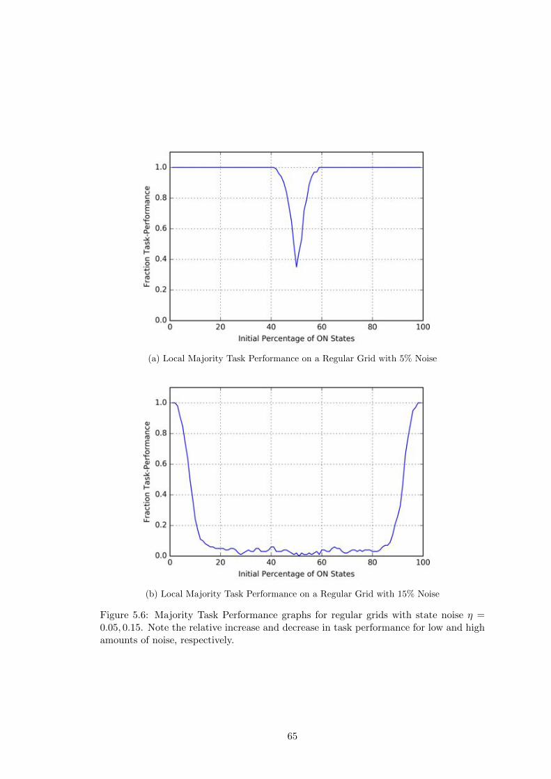
(a) Local Majority Task Performance on a Regular Grid with 5% Noise
(b) Local Majority Task Performance on a Regular Grid with 15% Noise
Figure 5.6: Majority Task Performance graphs for regular grids with state noise ⌘ =0.05, 0.15. Note the relative increase and decrease in task performance for low and highamounts of noise, respectively.
65
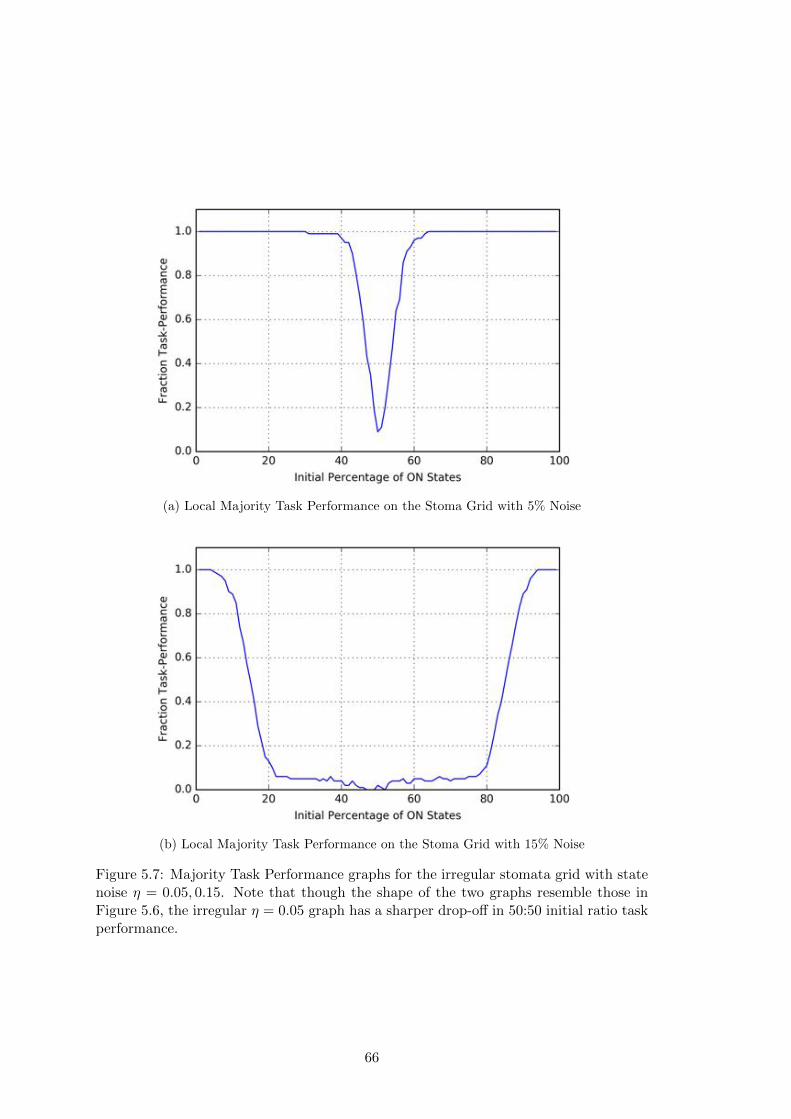
(a) Local Majority Task Performance on the Stoma Grid with 5% Noise
(b) Local Majority Task Performance on the Stoma Grid with 15% Noise
Figure 5.7: Majority Task Performance graphs for the irregular stomata grid with statenoise ⌘ = 0.05, 0.15. Note that though the shape of the two graphs resemble those inFigure 5.6, the irregular ⌘ = 0.05 graph has a sharper drop-o↵ in 50:50 initial ratio taskperformance.
66
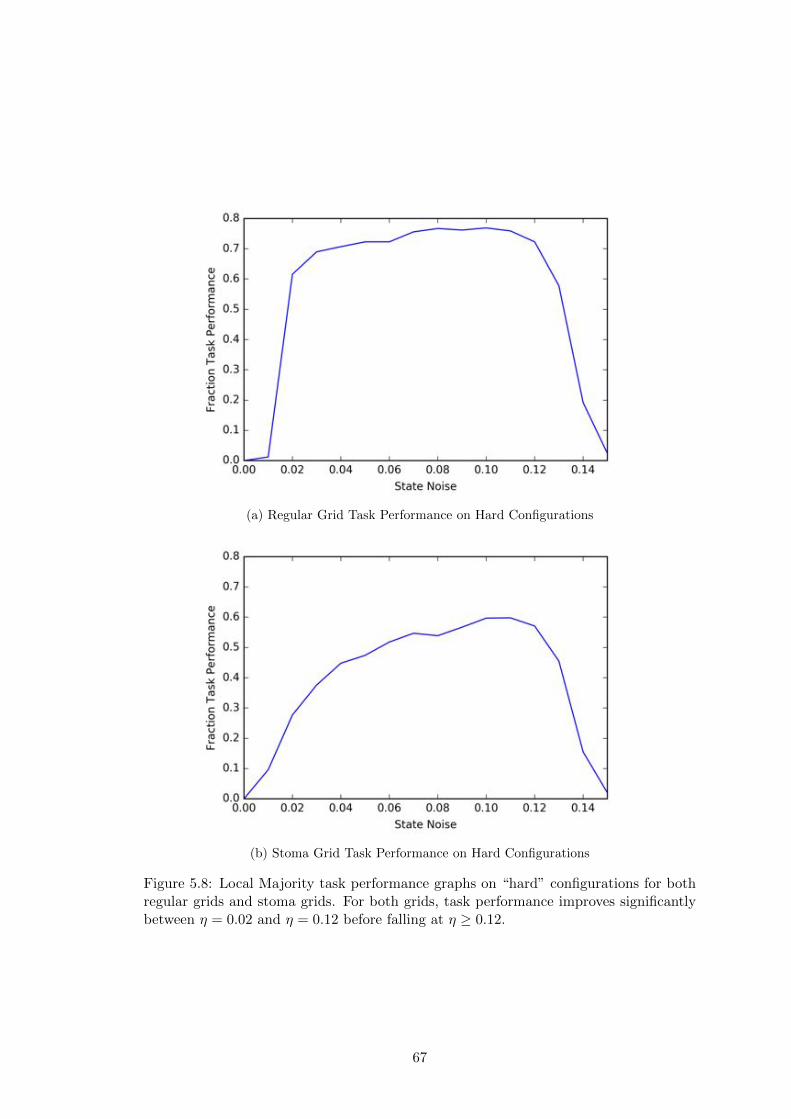
(a) Regular Grid Task Performance on Hard Configurations
(b) Stoma Grid Task Performance on Hard Configurations
Figure 5.8: Local Majority task performance graphs on “hard” configurations for bothregular grids and stoma grids. For both grids, task performance improves significantlybetween ⌘ = 0.02 and ⌘ = 0.12 before falling at ⌘ � 0.12.
67
Chapter 6
Lambda Degradation
Experiments
The � parameter as established by Langton is an e↵ective way to parameterize and
traverse the CA rule space. And though � may be too “coarse” of a parameter to
pinpoint precisely where the critical transition point is for particular class of CAs (see
Chapter 2.2.3), it is su�cient for detecting whether or not transition events can occur
for a given CA. Thus, we apply similar � analysis techniques used by Wootters and
Langton [26, 52] to irregular and degraded grids.
6.1 The Langton-Wootters � Profile
Our experiments build o↵ work by Wootters and Langton that specifically examine
K = 8, N = 5 CAs. As discussed in Chapter 2.2.2, Shannon entropy is often used
to measure the complexity of CA systems. Entropy is plotted against � in Wootters
and Langton’s experiments to produce what we call the Langton-Wootters Profile (LW
Profile), pictured in various forms from di↵erent table generation methods in Figure 6.1.
Generating the Langton-Wootters Profile
The table walk-through method for generating transition tables begins with a � tran-
sition function that has � = 0. Recalling the definition of � (Appendix A.1), � = 0
indicates that every rule in � maps to the quiescent state sq
. The � table is then
incremented to a higher � value by randomly replacing some of the transitions to sq
with transitions to the other possible states, uniformly chosen [26]. This table gener-
ation method has the e↵ect of modifying the “same” table, allowing us to track CA
behavior for individual runs of CA simulation. The LW Profile generated from the table
walk-through method is shown in Figure 6.1a.
The random table method for generating transition tables utilizes � as a sampling
probability. A � table entry is mapped to the quiescent state with probability 1 � �,
while a non-quiescent state is chosen uniformly from the other possible states with
probability � [26]. The LW Profile generated from the random table method is pictured
68
in Figure 6.1b. Also note that all � transition tables possess planar isotropy and strong
quiescence as detailed in Chapter 3.4.3.
Entropy is calculated using the equations shown in Appendix A.3. However, entropy
calculations are made only for the asymptotic behavior of a given CA simulation: each
CA simulation is run for 1,000 time steps, with entropy only measured after time step
500. So if a particular CA run has a lifetime of less than 500, its entropy value will be 0.
This manner of calculating asymptotic entropy leads to numerous entropy measurements
of 0, as pictured in both versions of the LW Profile. Also note that for K = 8, N = 5
CA, the maximum entropy is 3 with this maximum value occurring with a � value of
0.875 (Appendix B.2). Thus, all experiments with K = 8, N = 5 CA consider a range
of � values from � = 0.0 to � = 0.88.
Analysis of the Langton-Wootters Profile
Both renditions of the LW Profile indicate a bimodal distribution of entropy values,
with most data points either collected around H = 0 or H > 0.85. There is a region
where relatively few data points are observed over 0 � 0.6 and 0 < H 0.85. This
transition gap and bimodal distribution are indicators of a critical transition, illustrat-
ing the boundary between non-complex CA with low H values and complex CA with
much higher H values. This phenomenon is easy to see in Figure 6.1a, with individual
transition table runs showing a sharp increase in entropy from below the gap to above
the gap at a certain � value. This gap and sudden jump in H are indications that
critical transitions can occur in this particular class of CAs on regular grids. Thus, we
will utilize these features of the LW Profile to evaluate irregular grids on their ability
to support complex behavior. Also observe that entropy values converge rapidly when
� > 0.6, an indication of the shift of rule tables from complex (Class IV CA) to chaotic
(Class III CA). The most interesting action occurs when the variance of entropy values
is high, again corresponding to the critical transition gap and jump in entropy from
around H = 0.0 to H > 0.85. Langton discusses the “ceiling” of this transition region,
noting that H ⇡ 0.84 is the average entropy value of a commonly occurring low � chaotic
rule [26], another indication that the gap in data points for 0 < H 0.85 is indicative
of a critical transition.
6.2 � Profile of Irregular Grids
Experimental Setup
We utilize the table walk-through method when varying � for our experiments, as both
line and scatter plots can be generated from the resulting data. Though Wootters and
Langton run their CA simulations to 1,000 time steps, we saw no di↵erence in the shape
of the LW Profiles between trials with a maximum time step of 500 and trials with a
maximum time step of 1,000 (Figure 6.3), so in the interest of e�ciency we run our
experiments with a maximum of 500 time steps with an asymptotic threshold of 250
time steps. 100 individual table walk-through runs for K = 8, N = 5 CA are made,
69
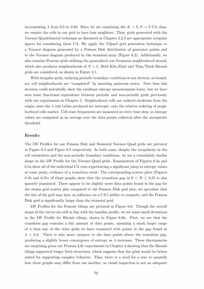
incrementing � from 0.0 to 0.88. Since we are examining the K = 8, N = 5 CA class,
we require the cells in our grid to have four neighbors. Thus, grids generated with the
Voronoi Quadrilateral technique as discussed in Chapter 3.2.3 are appropriate irregular
spaces for considering these CA. We apply the VQuad grid generation technique to
a Voronoi diagram generated by a Poisson Disk distribution of generator points and
to the Voronoi diagram produced by the stomatal array (Figure 6.2). Additionally, we
also examine Penrose grids utilizing the generalized von Neumann neighborhood stencil,
which also produces neighborhoods of N = 5. Both Kite/Dart and Thin/Thick Rhomb
grids are considered, as shown in Figure 4.1.
With irregular grids, inducing periodic boundary conditions is not obvious, so bound-
ary cell neighborhoods are “completed” by inserting quiescent states. Note that this
decision could potentially skew the resultant entropy measurements lower, but we have
seen some functional equivalence between periodic and non-periodic grids previously
with our experiments in Chapter 5. Neighborhood cells are ordered clockwise from the
origin; since the � rule tables produced are isotropic, only the relative ordering of neigh-
borhood cells matter. Cell state frequencies are measured at every time step, so entropy
values are computed as an average over the data points collected after the asymptotic
threshold.
Results
The LW Profiles for our Poisson Disk and Stomatal Voronoi Quad grids are pictured
in Figure 6.4 and Figure 6.5 respectively. In both cases, despite the irregularity in the
cell orientation and the non-periodic boundary conditions, we see a remarkably similar
shape in the LW Profile for the Voronoi Quad grids. Examination of Figures 6.4a and
6.5a show all of the individual CA runs experiencing a significant jump in entropy values
at some point, evidence of a transition event. The corresponding scatter plots (Figures
6.4b and 6.5b) of these graphs show that the transition gap in 0 < H 0.85 is also
sparsely populated. There appear to be slightly more data points found in the gap for
the stoma grid scatter plot compared to the Poisson Disk grid plot; we speculate that
the size of the grid may have an influence on a CA’s ability to compute, and the Poisson
Disk grid is significantly larger than the stomatal grid.
LW Profiles for the Penrose tilings are pictured in Figure 6.6. Though the overall
shape of the curves are still in line with the baseline profile, we see some small deviations
in the LW Profile for Rhomb tilings, shown in Figure 6.6b. First, we see that the
transition gap contains a fair amount of data points, spanning a much larger range
of � than any of the other grids we have examined with points in the gap found at
� < 0.2. There is also more variance in the data points above the transition gap,
producing a slightly looser convergence of entropy as � increases. These discrepancies
are surprising given our Penrose Life experiments in Chapter 4 showing that the Rhomb
tilings supported longer lived structures, which suggests that the grids would be better
suited for supporting complex behavior. Thus, there is a need for a way to quantify
how these graphs may di↵er from one another, as visual inspection is not an adequate
70
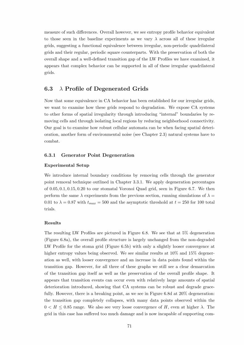
measure of such di↵erences. Overall however, we see entropy profile behavior equivalent
to those seen in the baseline experiments as we vary � across all of these irregular
grids, suggesting a functional equivalence between irregular, non-periodic quadrilateral
grids and their regular, periodic square counterparts. With the preservation of both the
overall shape and a well-defined transition gap of the LW Profiles we have examined, it
appears that complex behavior can be supported in all of these irregular quadrilateral
grids.
6.3 � Profile of Degenerated Grids
Now that some equivalence in CA behavior has been established for our irregular grids,
we want to examine how these grids respond to degradation. We expose CA systems
to other forms of spatial irregularity through introducing “internal” boundaries by re-
moving cells and through isolating local regions by reducing neighborhood connectivity.
Our goal is to examine how robust cellular automata can be when facing spatial deteri-
oration, another form of environmental noise (see Chapter 2.3) natural systems have to
combat.
6.3.1 Generator Point Degeneration
Experimental Setup
We introduce internal boundary conditions by removing cells through the generator
point removal technique outlined in Chapter 3.3.1. We apply degeneration percentages
of 0.05, 0.1, 0.15, 0.20 to our stomatal Voronoi Quad grid, seen in Figure 6.7. We then
perform the same � experiments from the previous section, running simulations of � =
0.01 to � = 0.87 with tmax
= 500 and the asymptotic threshold at t = 250 for 100 total
trials.
Results
The resulting LW Profiles are pictured in Figure 6.8. We see that at 5% degeneration
(Figure 6.8a), the overall profile structure is largely unchanged from the non-degraded
LW Profile for the stoma grid (Figure 6.5b) with only a slightly looser convergence at
higher entropy values being observed. We see similar results at 10% and 15% degener-
ation as well, with looser convergence and an increase in data points found within the
transition gap. However, for all three of these graphs we still see a clear demarcation
of the transition gap itself as well as the preservation of the overall profile shape. It
appears that transition events can occur even with relatively large amounts of spatial
deterioration introduced, showing that CA systems can be robust and degrade grace-
fully. However, there is a breaking point, as we see in Figure 6.8d at 20% degeneration:
the transition gap completely collapses, with many data points observed within the
0 < H 0.85 range. We also see very loose convergence of H, even at higher �. The
grid in this case has su↵ered too much damage and is now incapable of supporting com-
71
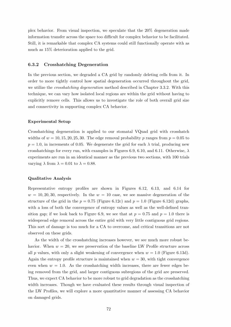
plex behavior. From visual inspection, we speculate that the 20% degeneration made
information transfer across the space too di�cult for complex behavior to be facilitated.
Still, it is remarkable that complex CA systems could still functionally operate with as
much as 15% deterioration applied to the grid.
6.3.2 Crosshatching Degeneration
In the previous section, we degraded a CA grid by randomly deleting cells from it. In
order to more tightly control how spatial degeneration occurred throughout the grid,
we utilize the crosshatching degeneration method described in Chapter 3.3.2. With this
technique, we can vary how isolated local regions are within the grid without having to
explicitly remove cells. This allows us to investigate the role of both overall grid size
and connectivity in supporting complex CA behavior.
Experimental Setup
Crosshatching degeneration is applied to our stomatal VQuad grid with crosshatch
widths of w = 10, 15, 20, 25, 30. The edge removal probability p ranges from p = 0.05 to
p = 1.0, in increments of 0.05. We degenerate the grid for each � trial, producing new
crosshatchings for every run, with examples in Figures 6.9, 6.10, and 6.11. Otherwise, �
experiments are run in an identical manner as the previous two sections, with 100 trials
varying � from � = 0.01 to � = 0.88.
Qualitative Analysis
Representative entropy profiles are shown in Figures 6.12, 6.13, and 6.14 for
w = 10, 20, 30, respectively. In the w = 10 case, we see massive degeneration of the
structure of the grid in the p = 0.75 (Figure 6.12c) and p = 1.0 (Figure 6.12d) graphs,
with a loss of both the convergence of entropy values as well as the well-defined tran-
sition gap; if we look back to Figure 6.9, we see that at p = 0.75 and p = 1.0 there is
widespread edge removal across the entire grid with very little contiguous grid regions.
This sort of damage is too much for a CA to overcome, and critical transitions are not
observed on these grids.
As the width of the crosshatching increases however, we see much more robust be-
havior. When w = 20, we see preservation of the baseline LW Profile structure across
all p values, with only a slight weakening of convergence when w = 1.0 (Figure 6.13d).
Again the entropy profile structure is maintained when w = 30, with tight convergence
even when w = 1.0. As the crosshatching width increases, there are fewer edges be-
ing removed from the grid, and larger contiguous subregions of the grid are preserved.
Thus, we expect CA behavior to be more robust to grid degradation as the crosshatching
width increases. Though we have evaluated these results through visual inspection of
the LW Profiles, we will explore a more quantitative manner of assessing CA behavior
on damaged grids.
72
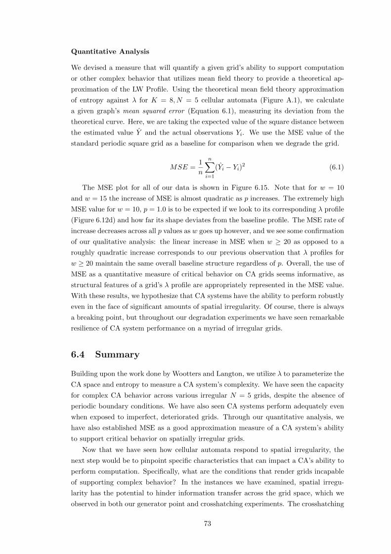
Quantitative Analysis
We devised a measure that will quantify a given grid’s ability to support computation
or other complex behavior that utilizes mean field theory to provide a theoretical ap-
proximation of the LW Profile. Using the theoretical mean field theory approximation
of entropy against � for K = 8, N = 5 cellular automata (Figure A.1), we calculate
a given graph’s mean squared error (Equation 6.1), measuring its deviation from the
theoretical curve. Here, we are taking the expected value of the square distance between
the estimated value Y and the actual observations Yi
. We use the MSE value of the
standard periodic square grid as a baseline for comparison when we degrade the grid.
MSE =1
n
nX
i=1
(Yi
� Yi
)2 (6.1)
The MSE plot for all of our data is shown in Figure 6.15. Note that for w = 10
and w = 15 the increase of MSE is almost quadratic as p increases. The extremely high
MSE value for w = 10, p = 1.0 is to be expected if we look to its corresponding � profile
(Figure 6.12d) and how far its shape deviates from the baseline profile. The MSE rate of
increase decreases across all p values as w goes up however, and we see some confirmation
of our qualitative analysis: the linear increase in MSE when w � 20 as opposed to a
roughly quadratic increase corresponds to our previous observation that � profiles for
w � 20 maintain the same overall baseline structure regardless of p. Overall, the use of
MSE as a quantitative measure of critical behavior on CA grids seems informative, as
structural features of a grid’s � profile are appropriately represented in the MSE value.
With these results, we hypothesize that CA systems have the ability to perform robustly
even in the face of significant amounts of spatial irregularity. Of course, there is always
a breaking point, but throughout our degradation experiments we have seen remarkable
resilience of CA system performance on a myriad of irregular grids.
6.4 Summary
Building upon the work done by Wootters and Langton, we utilize � to parameterize the
CA space and entropy to measure a CA system’s complexity. We have seen the capacity
for complex CA behavior across various irregular N = 5 grids, despite the absence of
periodic boundary conditions. We have also seen CA systems perform adequately even
when exposed to imperfect, deteriorated grids. Through our quantitative analysis, we
have also established MSE as a good approximation measure of a CA system’s ability
to support critical behavior on spatially irregular grids.
Now that we have seen how cellular automata respond to spatial irregularity, the
next step would be to pinpoint specific characteristics that can impact a CA’s ability to
perform computation. Specifically, what are the conditions that render grids incapable
of supporting complex behavior? In the instances we have examined, spatial irregu-
larity has the potential to hinder information transfer across the grid space, which we
observed in both our generator point and crosshatching experiments. The crosshatching
73

experiments also revealed the importance of having contiguous subregions within the
grid, as we saw robust critical behavior on grids with su�ciently wide crosshatches,
even when regions of the grid were largely disconnected from one another. We speculate
that spatial irregularity also impacts the ability of a CA system to store information;
long lasting coherent structures, such as oscillators in GoL require space to “take root”
within the grid in order to facilitate complex behavior. We have made a first step in
investigating the impact of spatial irregularity on cellular automata function, and fu-
ture work will look towards designing experiments and metrics that will consider these
questions concerning the foundations of CA computation with more precision.
74

Figures
(a) Walk-Through Langton-Wootters Profile
(b) Random Table and Theoretical Langton-Wootters Profile
Figure 6.1: Di↵erent forms of the LW Profile. Figure 6.1a shows 50 individual runs ofthe table-walk-through method of varying �. Figure 6.1b shows both a scatter plot ofdata points collected through the random-table method of varying � and the theoreticalLangton-Wootters Profile as predicted by mean field theory (Appendix A.5). Note howboth plots produce the same envelope of data points. Plots adapted from both Woottersand Langton, and Langton [26, 52].
75

(a) Voronoi Diagram of Stomatal Array
(b) VQuad Diagram of Stomatal Array
Figure 6.2: An illustration of the Voronoi representation of the stomatal array fromFigure 5.2 and the resultant Voronoi Quad grid.
76
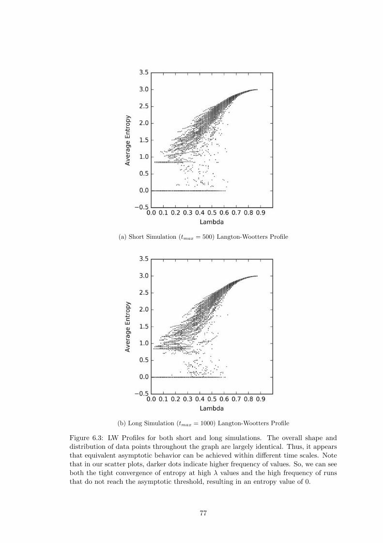
(a) Short Simulation (tmax
= 500) Langton-Wootters Profile
(b) Long Simulation (tmax
= 1000) Langton-Wootters Profile
Figure 6.3: LW Profiles for both short and long simulations. The overall shape anddistribution of data points throughout the graph are largely identical. Thus, it appearsthat equivalent asymptotic behavior can be achieved within di↵erent time scales. Notethat in our scatter plots, darker dots indicate higher frequency of values. So, we can seeboth the tight convergence of entropy at high � values and the high frequency of runsthat do not reach the asymptotic threshold, resulting in an entropy value of 0.
77
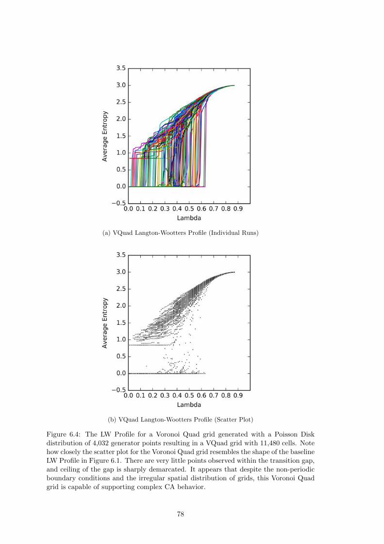
(a) VQuad Langton-Wootters Profile (Individual Runs)
(b) VQuad Langton-Wootters Profile (Scatter Plot)
Figure 6.4: The LW Profile for a Voronoi Quad grid generated with a Poisson Diskdistribution of 4,032 generator points resulting in a VQuad grid with 11,480 cells. Notehow closely the scatter plot for the Voronoi Quad grid resembles the shape of the baselineLW Profile in Figure 6.1. There are very little points observed within the transition gap,and ceiling of the gap is sharply demarcated. It appears that despite the non-periodicboundary conditions and the irregular spatial distribution of grids, this Voronoi Quadgrid is capable of supporting complex CA behavior.
78
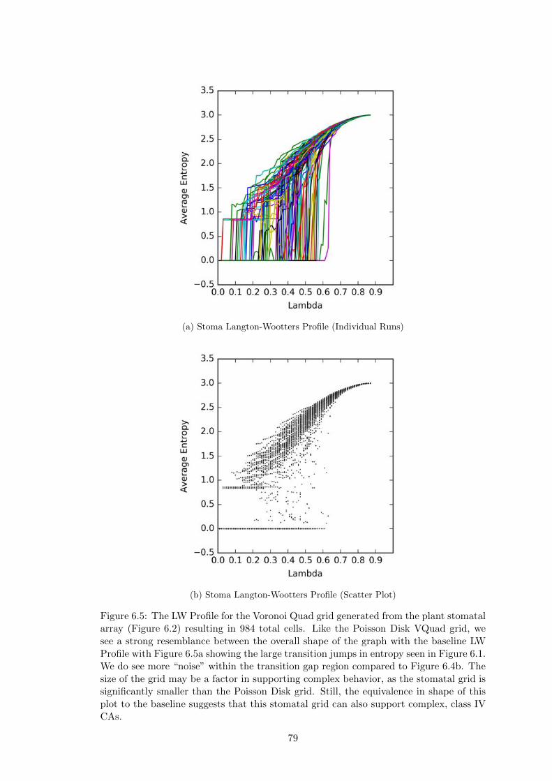
(a) Stoma Langton-Wootters Profile (Individual Runs)
(b) Stoma Langton-Wootters Profile (Scatter Plot)
Figure 6.5: The LW Profile for the Voronoi Quad grid generated from the plant stomatalarray (Figure 6.2) resulting in 984 total cells. Like the Poisson Disk VQuad grid, wesee a strong resemblance between the overall shape of the graph with the baseline LWProfile with Figure 6.5a showing the large transition jumps in entropy seen in Figure 6.1.We do see more “noise” within the transition gap region compared to Figure 6.4b. Thesize of the grid may be a factor in supporting complex behavior, as the stomatal grid issignificantly smaller than the Poisson Disk grid. Still, the equivalence in shape of thisplot to the baseline suggests that this stomatal grid can also support complex, class IVCAs.
79

(a) Kite/Dart Langton-Wootters Profile
(b) Thin/Thick Rhombus Langton-Wootters Profile
Figure 6.6: The LW Profile for both types of Penrose grids. Though both plots maintainthe same overall shape as the baseline LW Profile, there appears to be significantlymore noise throughout the entire graph for the Rhomb grid, with more points withinthe transition gap and looser convergence to the overall profile shape at entropy valuesabove the transition gap. This is surprising given that our Penrose Life experimentsshowed the Rhomb tilings supporting longer living Life structures than the Kites/Darttiling, suggesting that perhaps the Rhomb tilings would be better suited for supportingcomplex CA behavior in general.
80
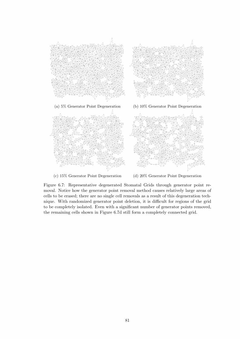
(a) 5% Generator Point Degeneration (b) 10% Generator Point Degeneration
(c) 15% Generator Point Degeneration (d) 20% Generator Point Degeneration
Figure 6.7: Representative degenerated Stomatal Grids through generator point re-moval. Notice how the generator point removal method causes relatively large areas ofcells to be erased; there are no single cell removals as a result of this degeneration tech-nique. With randomized generator point deletion, it is di�cult for regions of the gridto be completely isolated. Even with a significant number of generator points removed,the remaining cells shown in Figure 6.7d still form a completely connected grid.
81
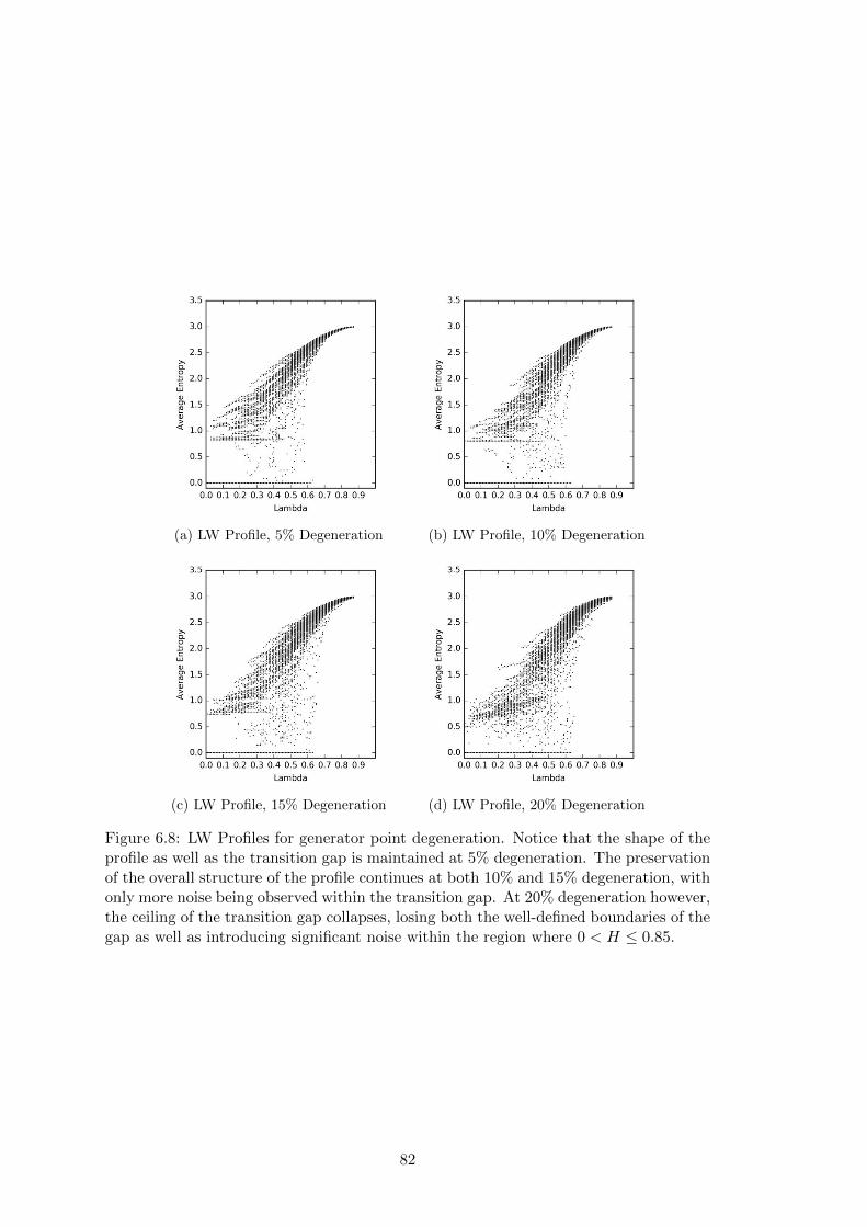
(a) LW Profile, 5% Degeneration (b) LW Profile, 10% Degeneration
(c) LW Profile, 15% Degeneration (d) LW Profile, 20% Degeneration
Figure 6.8: LW Profiles for generator point degeneration. Notice that the shape of theprofile as well as the transition gap is maintained at 5% degeneration. The preservationof the overall structure of the profile continues at both 10% and 15% degeneration, withonly more noise being observed within the transition gap. At 20% degeneration however,the ceiling of the transition gap collapses, losing both the well-defined boundaries of thegap as well as introducing significant noise within the region where 0 < H 0.85.
82

(a) Crosshatch Degeneration, w = 10, p =0.25
(b) Crosshatch Degeneration, w = 10, p =0.50
(c) Crosshatch Degeneration, w = 10, p =0.75
(d) Crosshatch Degeneration, w = 10, p =1.0
Figure 6.9: Representative grids for crosshatching degeneration w = 10 applied to thestomatal VQuad grid. Notice how at p = 1.0, the crosshatchings are placed so closetogether that subregion partitions are not well-defined.
83
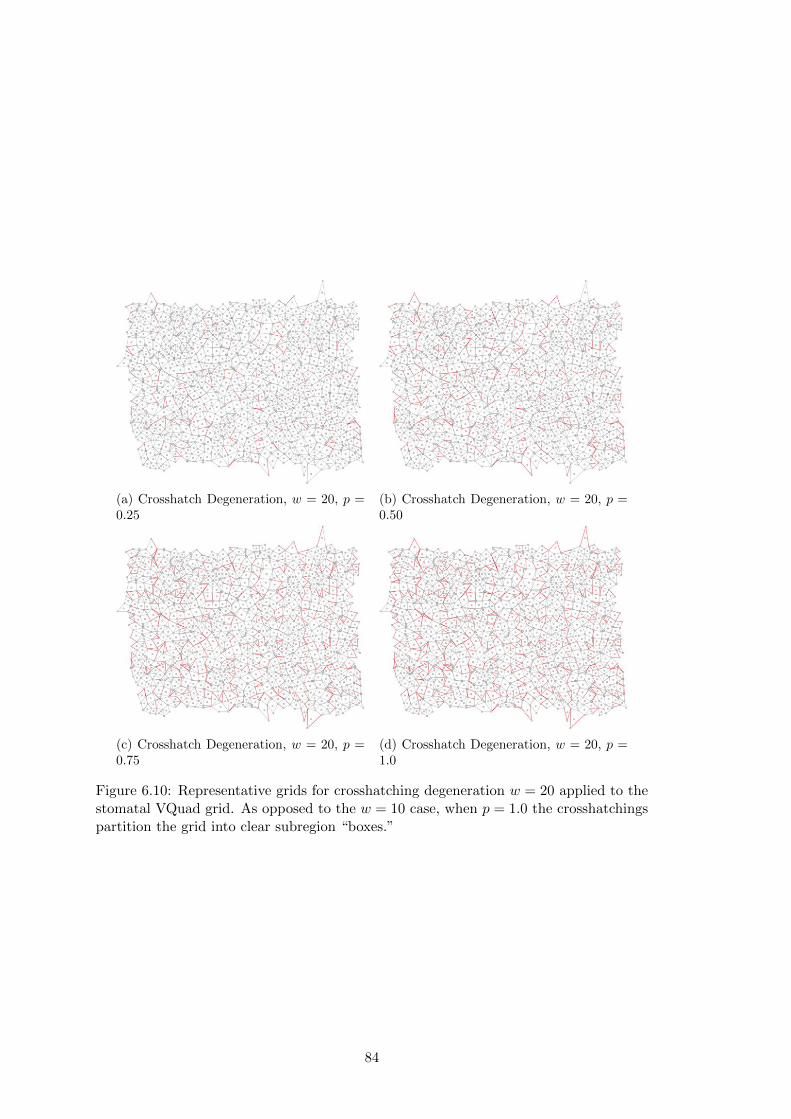
(a) Crosshatch Degeneration, w = 20, p =0.25
(b) Crosshatch Degeneration, w = 20, p =0.50
(c) Crosshatch Degeneration, w = 20, p =0.75
(d) Crosshatch Degeneration, w = 20, p =1.0
Figure 6.10: Representative grids for crosshatching degeneration w = 20 applied to thestomatal VQuad grid. As opposed to the w = 10 case, when p = 1.0 the crosshatchingspartition the grid into clear subregion “boxes.”
84

(a) Crosshatch Degeneration, w = 30, p =0.25
(b) Crosshatch Degeneration, w = 30, p =0.50
(c) Crosshatch Degeneration, w = 30, p =0.75
(d) Crosshatch Degeneration, w = 30, p =1.0
Figure 6.11: Representative grids for crosshatching degeneration w = 20 applied to thestomatal VQuad grid. Again when p = 1.0, the crosshatchings partition the grid intosquare subregions.
85
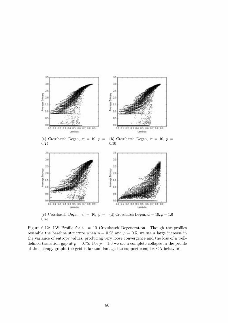
(a) Crosshatch Degen, w = 10, p =0.25
(b) Crosshatch Degen, w = 10, p =0.50
(c) Crosshatch Degen, w = 10, p =0.75
(d) Crosshatch Degen, w = 10, p = 1.0
Figure 6.12: LW Profile for w = 10 Crosshatch Degeneration. Though the profilesresemble the baseline structure when p = 0.25 and p = 0.5, we see a large increase inthe variance of entropy values, producing very loose convergence and the loss of a well-defined transition gap at p = 0.75. For p = 1.0 we see a complete collapse in the profileof the entropy graph; the grid is far too damaged to support complex CA behavior.
86
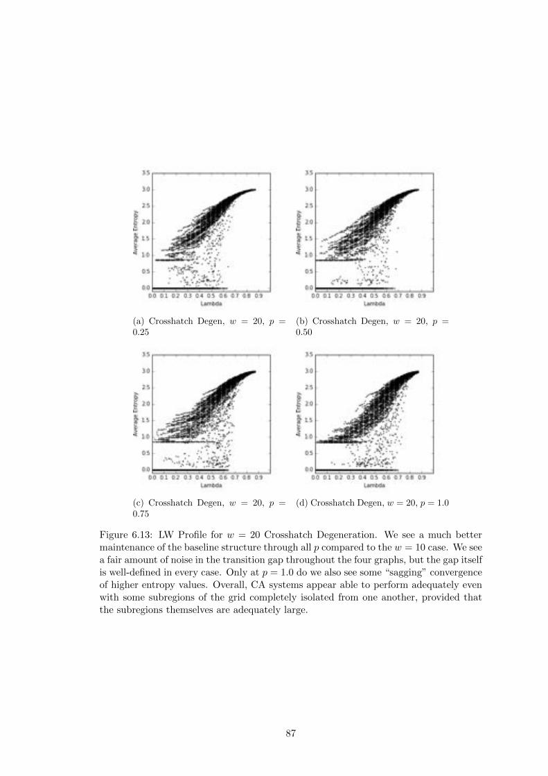
(a) Crosshatch Degen, w = 20, p =0.25
(b) Crosshatch Degen, w = 20, p =0.50
(c) Crosshatch Degen, w = 20, p =0.75
(d) Crosshatch Degen, w = 20, p = 1.0
Figure 6.13: LW Profile for w = 20 Crosshatch Degeneration. We see a much bettermaintenance of the baseline structure through all p compared to the w = 10 case. We seea fair amount of noise in the transition gap throughout the four graphs, but the gap itselfis well-defined in every case. Only at p = 1.0 do we also see some “sagging” convergenceof higher entropy values. Overall, CA systems appear able to perform adequately evenwith some subregions of the grid completely isolated from one another, provided thatthe subregions themselves are adequately large.
87

(a) Crosshatch Degen, w = 30, p =0.25
(b) Crosshatch Degen, w = 30, p =0.50
(c) Crosshatch Degen, w = 30, p =0.75
(d) Crosshatch Degen, w = 30, p = 1.0
Figure 6.14: LW Profile for w = 30 Crosshatch Degeneration. Again, overall structureof the entropy profile is maintained at all p, with the only deviations being data pointsobserved in the transition gap. We see tight convergence of entropy values in all thegraphs, even when p = 1.0. It appears that larger crosshatching widths impact thebehavior of CA systems less; this is unsurprising as there are less edges removed fromthe grid and larger subregions being created as a result of the wider width.
88
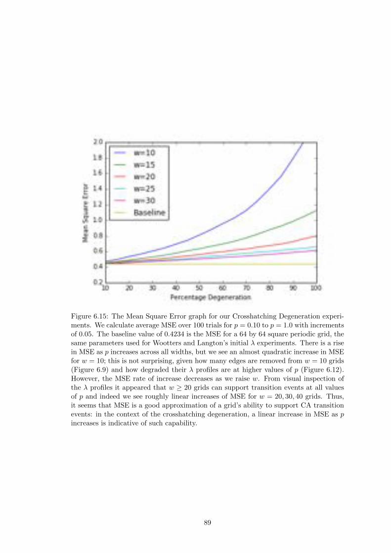
Figure 6.15: The Mean Square Error graph for our Crosshatching Degeneration experi-ments. We calculate average MSE over 100 trials for p = 0.10 to p = 1.0 with incrementsof 0.05. The baseline value of 0.4234 is the MSE for a 64 by 64 square periodic grid, thesame parameters used for Wootters and Langton’s initial � experiments. There is a risein MSE as p increases across all widths, but we see an almost quadratic increase in MSEfor w = 10; this is not surprising, given how many edges are removed from w = 10 grids(Figure 6.9) and how degraded their � profiles are at higher values of p (Figure 6.12).However, the MSE rate of increase decreases as we raise w. From visual inspection ofthe � profiles it appeared that w � 20 grids can support transition events at all valuesof p and indeed we see roughly linear increases of MSE for w = 20, 30, 40 grids. Thus,it seems that MSE is a good approximation of a grid’s ability to support CA transitionevents: in the context of the crosshatching degeneration, a linear increase in MSE as pincreases is indicative of such capability.
89
Chapter 7
Future Work
Throughout the previous chapters, we have considered how spatial irregularity impacts
complex CA behavior. Our exploratory experiments have suggested that CA systems are
relatively robust to nonuniform spatial environments and can even perform adequately
on degraded or damaged grids. In some instances, we see that spatial irregularity even
facilitates complex behavior. However, all of these conclusions are qualified by the
fact that we have only examined a few specific CA domains, utilizing metrics that
are considered to capture broad, general characteristics of CA function rather than
pinpointing specifics of critical CA function. Thus, we will re-evaluate our results and
consider some future directions expanding on the work we have done.
7.1 Evaluation and Critique of Our Results
Our experiments on Penrose Life, the Majority Task and � have all pointed to the
idea that CA systems can operate on nonuniform grids. However, as we have noted in
our discussions, there could be other properties that impact CA behavior that change
alongside the spatial noise we introduce. The most prominent of such properties that
we need to be aware of is neighborhood size. Previous work by Flache and Hegselmann
has suggested that the connectivity of a given cell is a major driving factor for variations
on CA system behavior [17], and the impact of irregular cells could simply be due to
the introduction of variable neighborhood degree, not because of spatial non-uniformity
itself. We see a similar sort of e↵ect in the experiments we have run ourselves, as Pen-
rose Life on Thin/Thick Rhomb grids had higher average lifetimes than on Kite/Dart
grids (Chapter 4.1) but also had higher average neighborhood sizes (Chapter 4.3) when
using a generalized Moore neighborhood stencil. It is unclear what governs the Penrose
Life average lifetimes in this situation, and when we consider Rhombs and Kites/Darts
for � experiments with a von Neumann neighborhood (producing the same sized neigh-
borhoods), we see that Kite/Dart grids perhaps support complex behavior better than
Rhomb grids (Figure 6.6). Thus we need to carefully control the parameters of our
experiments to ensure that connectivity and neighborhood size do not skew our results.
Performing more experiments on specific classes of CAs, like our � investigations, where
the neighborhood size is fixed is a good way to both parameterize the CA space and
90
reduce any potential connectivity e↵ects.
Another characteristic of irregular grids we have to consider carefully is the grid
boundary condition. Though traditional CA systems have the advantage of complete
neighborhoods at every cell due to periodic square lattice boundaries, natural dynamic
systems have to deal with the fact that some neighborhoods will be incomplete at the
borders since they operate in a bounded space. We have seen that despite this limita-
tion, CA systems on irregular grids can still perform comparably to their counterparts
on regular, periodic grids. We speculate that boundaries could act as regions of “sta-
bility” where neighborhood interactions are simpler and more consistent than within
central regions of the grid: for example, we often saw long-living Penrose Life structures
utilizing boundary cells to their advantage (Chapter 4.2). Then again, it is not clear
how the boundary impacts a CA system’s behavior in other domains, as majority task
performance decreased on regular but non-periodic grids (Figure 5.5) in comparison to
periodic grids, while irregular non-periodic grids perform comparably to the regular, pe-
riodic baseline case (Figure 5.4). Internal boundary conditions must also be considered,
as they are introduced when grids are spatially degraded, such as when cells are re-
moved from the grid (Chapter 6.3.1). Ultimately, boundary conditions are unavoidable
when considering spatial irregularities in natural dynamic systems and appear to play
an important role in the type of CA behavior a space can support, so future experiments
should isolate and attempt to distill the specific e↵ects of a grid’s boundary.
7.2 Measuring Information Transfer
As we discussed in Chapter 4, spatial irregularity can have a large impact on the ability
to transfer information across the grid space, a requisite property for supporting compu-
tation in a CA system. Though we have made some indirect observations on information
transfer in our experiments by looking at Penrose Life lifetimes and asymptotic entropy,
more direct measurements of information transfer should be made. Some spatial prop-
erties to consider would be the connectedness of the grid as well as the geodesic distance,
or shortest path between two cells on the grid. In some of the degenerated grids we have
considered in our � experiments, we suspect that one of the main factors that causes the
deterioration of the CA’s � profile is due to increased di�culty in information transfer.
In particular, it would be interesting to measure the geodesic distances for the grids in
Figure 3.7 to see if there are correlations between the average geodesic distances for all
pairs of cells and the degree of degradation seen in their respective � profiles.
Another factor to consider is the speed at which information travels across the grid
space. Though used primarily for measuring the “variance” of CA behavior, the �
parameter (Chapter 2.2.2, Appendix A.2) can also be utilized to quantify the average
propagation speed of di↵erence patterns traveling across the space. Adapting � to
two-dimensional, irregular grids could not only help parameterize the CA space we are
considering but also characterize how fast particles travel within the space. Measuring
the rate of information transfer is particularly important for irregular grids, as though
91
the “speed of light,” or maximum information transfer speed, is constant across a regular
CA grid, due to variability in spatial orientation and neighborhood sizes it may not be
constant on irregular grids. And since � is often high within the critical transition region
of CA systems [32], we hypothesize that there may be a minimum speed of light that is
required in order to support complex behavior. Though generalizing � two dimensions
will require some thought, especially given that the metric relies on global directional
orientation (compass directions) which may not be well-defined for irregular grids, we
believe an investigation of � will ultimately be fruitful in pinpointing the impact of
spatial irregularities on information transfer and ultimately complex CA behavior.
7.3 Consideration of Continuous Dynamical Systems
Another assumption we make when modeling natural dynamic systems is that discrete
CA rule transitions can adequately describe the change and behavior of such systems.
Clearly dynamic systems in the wild operate in a continuous environment, and though
some equivalence between discrete rules and continuous transitions have been estab-
lished (Messinger et al. found through time series analysis that discrete time granularity
provides an adequate mapping to continuous stomatal behavior [30]), it still would be
fruitful to consider continuous CA models. In particular, since we utilize Voronoi dia-
grams, which respect Euclidean distance, as our primary means for introducing spatial
irregularity, the next natural step would be to consider rule tables that respect Euclidean
distance as well.
In SmoothLife (Chapter 2.4.2), we have seen neighborhood “stencils” defined by a
distance metric and transition rules defined by a continuous curve (Figure 7.1). In-
stead of having set neighborhood stencils, we could investigate continuous CA models
where neighborhoods are defined by an area of influence that diminishes, perhaps with
Gaussian smoothing, the farther a cell sits from the center cell. Similarly, transition
rules can be defined in terms of a function rather than a discrete table, allowing for
continuous changes in CA cell states. These modifications would serve the same under-
lying purpose as our spatial irregularity experiments have: to examine whether our CA
models are adequate in representing the fundamental properties of natural systems in
order to better understand their behavior. The goal again would be investigate whether
there is a functional equivalence between more traditional CA models and the “smooth”
representations we have proposed.
7.4 Criticality under Microscope: Other CA Metrics to
Consider
Though we have examined the canonical CA space parameter � and devised our own
approximation of complexity through Mean Square Error (Chapter 6.3.2), these metrics
only paint a broad picture of critical behavior. Indeed, though we have established that
critical behavior is possible on spatially irregular grids, we have yet to explore deeply
92

the impact of such irregularity on CA function. As we discussed in Chapter 2.2.3, the
edge of chaos may be more subtle than simply identifying the boundary between ordered
and chaotic CAs by jumps in entropy. Thus, to continue this work, we would look to
finer-grained metrics that could potentially allow us to parameterize CA critical regions
in order to traverse it in greater detail.
One measure that has been shown to be a good indicator of critical behavior is the
power spectral density, which describes the distribution of frequency components of some
signal. In the case of cellular automata, the spectral density S(f) is the squared sum
of the Fourier transformation of a time series of cell state values [36]. Critical behavior
in dynamic systems is often marked by 1/f fluctuation, where the power spectrum as
a function of a frequency f behaves like 1/f (Figure 7.2). In particular, self-organized
criticality in dynamic systems, where critical state is achieved regardless of initial state
conditions, is found to correspond with such power spectra fluctuations [5]. Ninagawa
et al. have shown that the 1/f fluctuation sharply di↵erentiates the Game of Life from
rules that have similar � values but ultimately do not produce complex behavior (Fig-
ure 7.3) [36]. Such power spectra behavior is also often accompanied by self-similarity
and fractal structures, visual and spatial indicators of critical behavior. Thus, applying
power spectra analysis to the spatially irregular grids would give us a deeper and more
detailed statistical analysis of the critical region and perhaps even a greater understand-
ing of what conditions cause critical phenomenon to emerge.
Another measure that could give us insight into the internal structure of the critical
region is a basin of attraction. Since CA systems are deterministic, they follow a unique
trajectory from a given initial state. Grid states have the potential to repeat, settling
on an attractor cycle that represents a particular CA’s stable state. Given the CA’s rule
table, we can then trace backwards the states that could lead to an attractor state, until
we reach aGarden of Eden state that has no predecessor state. The connected graph that
results from tracing states from the attractor back to Garden of Eden states is the basin
of attraction for a particular CA system. This structure allows us to categorize the global
characteristics of a CA system and can help us determine whether information processing
is possible. For example, Wuensche et al. utilize attractor basins to identify whether a
given CA’s dynamics can support glider-like structures: such attractor basins have long
transient paths to the attractor cycles with relatively small periods [53] (Figure 7.4).
Interestingly, Wuensche et al. have also used attractor basin properties to automatically
classify CA systems: for example, complex CA often produce attractor basins that have
an in-degree frequency that follows a power law distribution as we previously discussed.
Though the attractor basin portrait of a CA is an immensely useful tool for examining
CA behavior, adapting the measure to two dimensions and to irregular grids could
pose a challenge, as local neighborhood configurations are now often unique and the
overall state space is much larger. Still, we believe that further work in developing such
generalizations of attractor basins would allow us to take a closer examination of CA
critical region features that could characterize such systems beyond just average entropy.
93
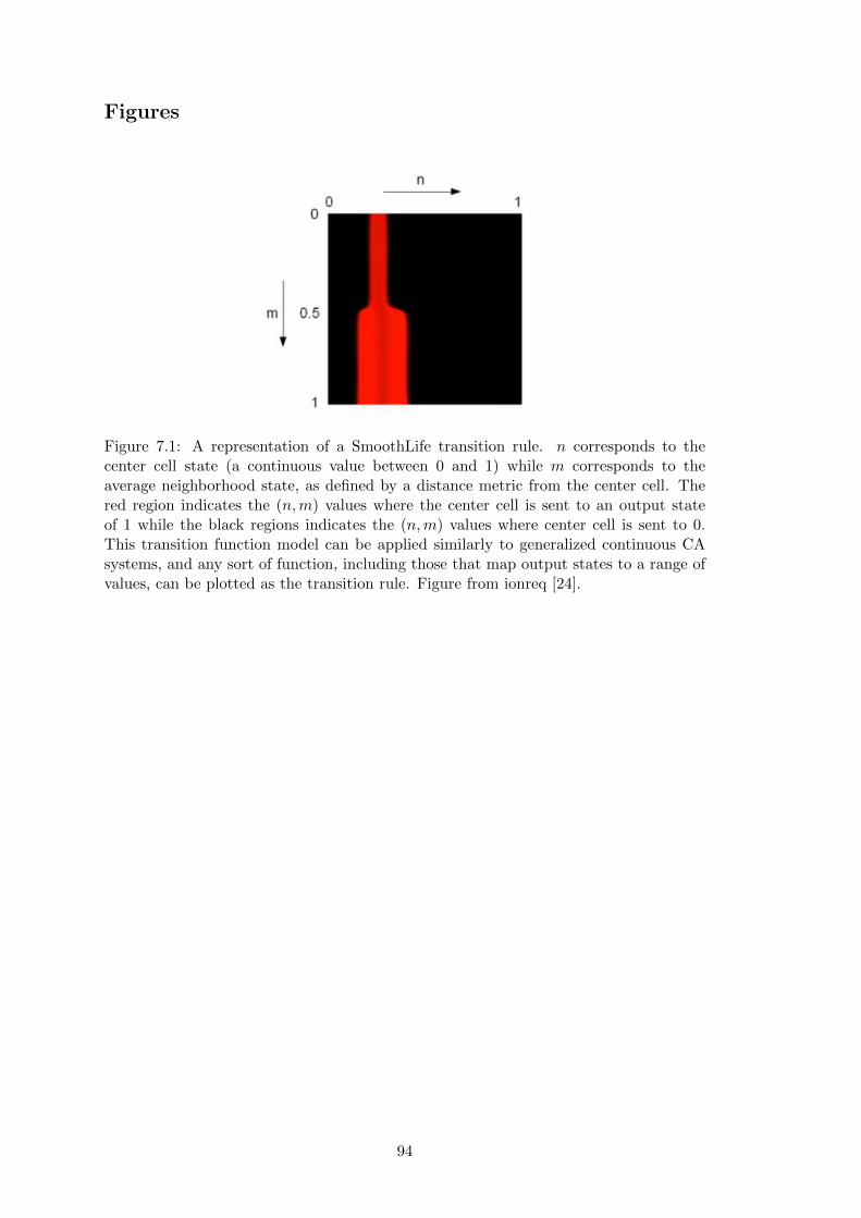
Figures
Figure 7.1: A representation of a SmoothLife transition rule. n corresponds to thecenter cell state (a continuous value between 0 and 1) while m corresponds to theaverage neighborhood state, as defined by a distance metric from the center cell. Thered region indicates the (n,m) values where the center cell is sent to an output stateof 1 while the black regions indicates the (n,m) values where center cell is sent to 0.This transition function model can be applied similarly to generalized continuous CAsystems, and any sort of function, including those that map output states to a range ofvalues, can be plotted as the transition rule. Figure from ionreq [24].
94
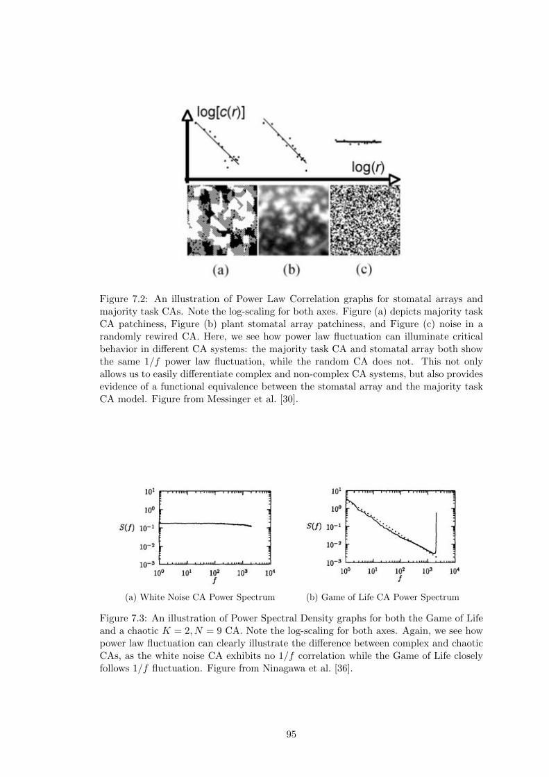
Figure 7.2: An illustration of Power Law Correlation graphs for stomatal arrays andmajority task CAs. Note the log-scaling for both axes. Figure (a) depicts majority taskCA patchiness, Figure (b) plant stomatal array patchiness, and Figure (c) noise in arandomly rewired CA. Here, we see how power law fluctuation can illuminate criticalbehavior in di↵erent CA systems: the majority task CA and stomatal array both showthe same 1/f power law fluctuation, while the random CA does not. This not onlyallows us to easily di↵erentiate complex and non-complex CA systems, but also providesevidence of a functional equivalence between the stomatal array and the majority taskCA model. Figure from Messinger et al. [30].
(a) White Noise CA Power Spectrum (b) Game of Life CA Power Spectrum
Figure 7.3: An illustration of Power Spectral Density graphs for both the Game of Lifeand a chaotic K = 2, N = 9 CA. Note the log-scaling for both axes. Again, we see howpower law fluctuation can clearly illustrate the di↵erence between complex and chaoticCAs, as the white noise CA exhibits no 1/f correlation while the Game of Life closelyfollows 1/f fluctuation. Figure from Ninagawa et al. [36].
95
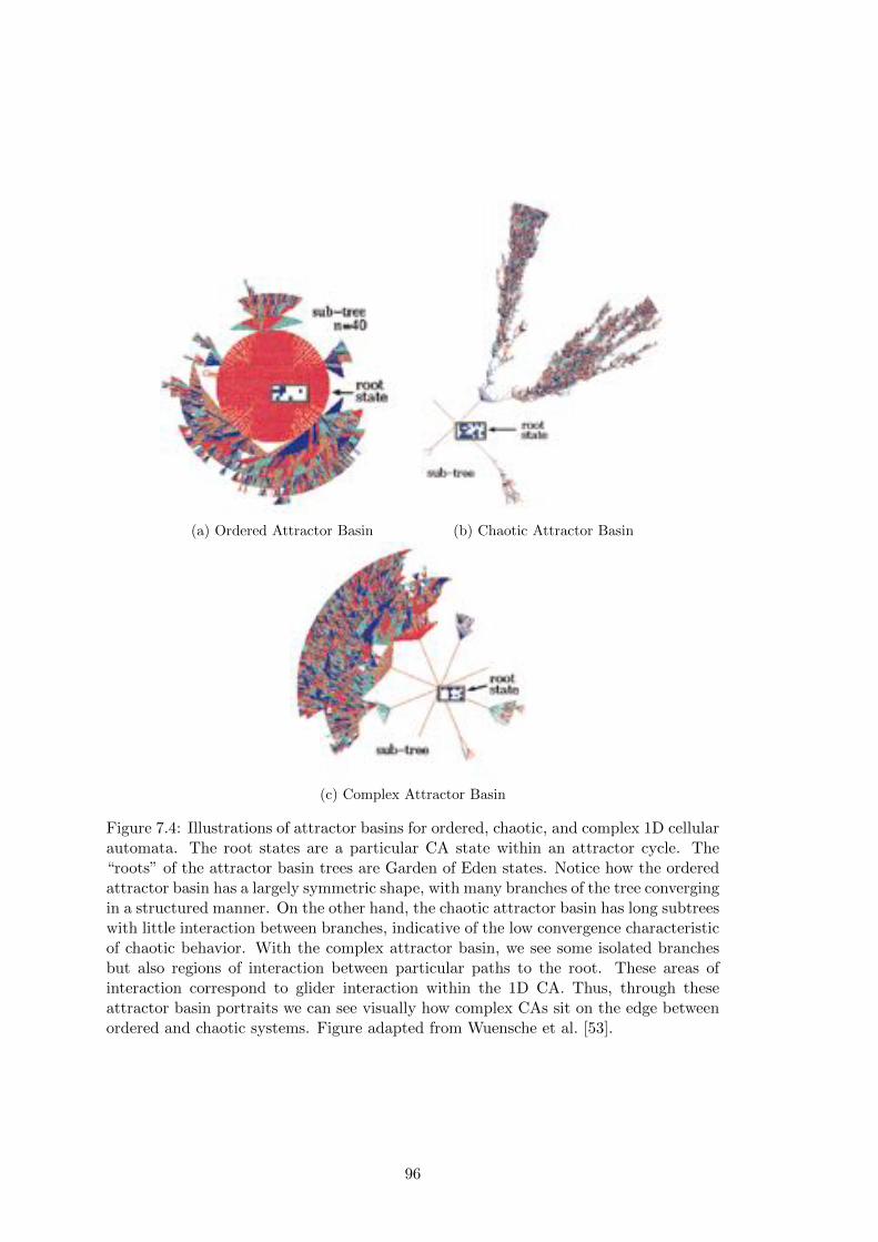
(a) Ordered Attractor Basin (b) Chaotic Attractor Basin
(c) Complex Attractor Basin
Figure 7.4: Illustrations of attractor basins for ordered, chaotic, and complex 1D cellularautomata. The root states are a particular CA state within an attractor cycle. The“roots” of the attractor basin trees are Garden of Eden states. Notice how the orderedattractor basin has a largely symmetric shape, with many branches of the tree convergingin a structured manner. On the other hand, the chaotic attractor basin has long subtreeswith little interaction between branches, indicative of the low convergence characteristicof chaotic behavior. With the complex attractor basin, we see some isolated branchesbut also regions of interaction between particular paths to the root. These areas ofinteraction correspond to glider interaction within the 1D CA. Thus, through theseattractor basin portraits we can see visually how complex CAs sit on the edge betweenordered and chaotic systems. Figure adapted from Wuensche et al. [53].
96

Chapter 8
Conclusions
From the experiments we have conducted, we have tentatively shown that CA systems
are robust to spatial irregularity. It appears that features of regular grids that initially
seemed crucial for supporting CA behavior such as uniform neighborhood sizes and
periodic boundaries are in fact not required for supporting complex behavior. Though
we have relaxed many of the spatial assumptions made in traditional CA systems, both
our majority task and � experiments have produced remarkably similar results to the
regular grid case.
What do these findings tell us about equivalences between spatially di↵erent CA
grids? Though our initial results are promising and suggest that there may at least
be a rough functional equivalence between regular and irregular grids, more work has
to be done in order to pinpoint the impact of specific spatial characteristics on CA
function. We have shown across all three of our experimental threads that the function
of domain-specific cellular automata on regular grids have strong qualitative similarities
with CA function on irregular grids, but even our initial quantitative measurements show
some significant di↵erences. Additionally, it is clear that irregular grids in general more
accurately represent the environment natural dynamic systems operate in, specifically
with their inclusion of a spatial boundary. Thus, though perhaps regular grids may serve
as an adequate simulacrum of the spatial environments encountered by natural CA-like
systems in simple modeling cases, in order to get to the heart of how these systems
operate and process information we must carefully consider the properties of non-uniform
spatial environments. The fundamental goal is to pinpoint how computation can arise
in such systems.
We can take two stances on computation in cellular automata: we can view initial
configurations as input to the CA “computer,” or we can view initial configurations
as computers themselves embedded in the logical universe provided by the cellular au-
tomata [26]. The transition rules in the first view constitute the algorithm defined by
the CA, while the in the second view they constitute the “physics” that the CA governs
within the space. Though we traditionally think of cellular automata in terms of the first
viewpoint, in order to truly understand the foundations of computation in decentralized
dynamic systems the second viewpoint must be adopted. We can easily embed universal
computers within the confines of CA transition rule and initial configuration definitions,
97
but what is more interesting is how complex behavior can emerge from the natural me-
chanics of the CA system, which is certainly more attuned with how dynamics occur in
nature. Here, the spatial configuration of a CA space becomes vitally important: each
variation and imperfection in the grid will shape what sort of intrinsic computational
mechanisms are possible within the context of the given cellular automaton.
Ultimately, we are trying to understand how natural dynamic environments can
support inherent computation without the rigid restrictions of regularity. The hope is
that knowledge of how these natural systems achieve robust behavior will inform us on
how to create computational architectures that do not depend on precision and leave
a razor-thin margin of error. We have taken the first step in attempting to explain
how decentralized natural systems handle and embrace imperfections in the pursuit of
harnessing the power of such computational systems in the wild.
98

Appendix A
Definitions of Criticality Metrics
A.1 Lambda
(From Langton [26]) Given a cellular automata with cell states ⌃ (K = |⌃|) and N
neighbors, pick an arbitrary state s 2 ⌃ and call it the quiescent state sq
. Let n be
the number of transitions some transition function � maps to sq
. Pick the remaining
KN � n transitions to be distributed uniformly over the other K � 1 states. Then � is:
� =KN � n
KN
(A.1.1)
A.2 Gamma
(From Li et al. [28]) First, we define the left-moving di↵erence rate for one-dimensional
CA by taking a configuration a = {...a�1, a0, a1...} and constructing another configura-
tion a0 = {...a0�1, a00, a
01...} with a
i
= a0i
for i < 0, ai
6= a0i
for i = 0 and a0i
randomly
chosen for i > 0. The di↵erence pattern at time step t for a given cell i is defined as
�ti
= 0 if ati
= a0t
i
and �ti
= 1 otherwise. The left front of the di↵erence pattern is
itleft
= min{i|�ti
= 1}. Thus the left-moving di↵erence rate �left
is:
�left
(a) = lim⌧!1
=i⌧left
� i⌧+t
left
t(A.2.1)
Similarly, the right-moving di↵erence rate is defined with ai
= a0i
for i > 0, ai
6= a0i
for i = 0 and a0i
randomly chosen for i < 0. The right front is iright
= max{i|�ti
= 1}.Then �
right
is:
�right
(a) = lim⌧!1
=i⌧+t
right
� i⌧right
t(A.2.2)
The overall di↵erence spreading rate � is then:
�(a) = �left
(a) + �right
(a) (A.2.3)
99

A.3 Shannon Entropy
(From Li et al. [28]) Given some discrete probability distribution {pi
}, the Shannon
entropy H is defined as:
H =X
i
pi
log(pi
) (A.3.1)
The single cell spatial entropy is calculated by defining a probability distribution
counting the frequency of occurrence of all states in ⌃ for a set number of time steps.
Let {ci
} for i = 1...K be the set of all counts, where ci
is the number of times state
i 2 ⌃ occurs. Then the probability distribution is:
{pi
} =
(ciPj
cj
)(A.3.2)
A.4 Mutual Information
(From Li et al. [28]) Given two probability distributions {pi
} and {pj
} as well as their
joint distribution {pij
}, we define the mutual information M as:
M =X
i
X
j
pij
logpij
pi
pj
(A.4.1)
We can apply mutual information to spatial-temporal patterns by defining the two
probability distributions as the frequency of having a particular cell state on two sites
separated by some distance d. The mutual information between two sites of any spatial-
temporal distance can be computed.
A.5 Mean Field Theory Estimates
(From Li et al. [28]) Given a 1D cellular automata with K = 2 and N = 2r+ 1, we can
obtain some estimates of both �c
and �. �c
can be estimated by:
�c
=1
2� 1
2
r1� 2
r + 1(A.5.1)
In order to estimate �, first calculate � using the cellular automata’s transition rules
�. Then:
� =(2r + 2)�� (2r + 2)�2 � 1
�(1� �)(A.5.2)
We can also make a rough first approximation of entropy H using simple mean field
theory. For a K = k CA at a given � value, we estimate H as:
Hm.f.
= �(1� �) log(1� �)� � log�
k � 1(A.5.3)
100

Wootters and Langton utilize mean field theory to make a more detailed estimate
of the entropy H of 2D cellular automata with K = 8 and N = 5 [52]. Let v be the
density of the quiescent state sq
in the spatial configuration, so v = 1 would indicate a
configuration of all sq
. K = 8, N = 5 cellular automata in their steady state will satisfy
the following equation:
v = v5 + (1� v5)(1� �) (A.5.4)
Then, assuming that the other seven states appear equally often in the transition rules
�, we can estimate H:
H = �v log v + 7
✓1� v
7
◆log
✓1� v
7
◆�(A.5.5)
This estimate for entropy is plotted in Figure A.1.
101
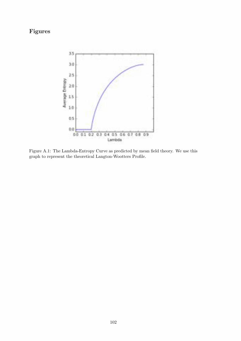
Figures
Figure A.1: The Lambda-Entropy Curve as predicted by mean field theory. We use thisgraph to represent the theoretical Langton-Wootters Profile.
102
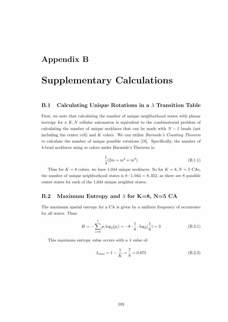
Appendix B
Supplementary Calculations
B.1 Calculating Unique Rotations in a � Transition Table
First, we note that calculating the number of unique neighborhood states with planar
isotropy for a K,N cellular automaton is equivalent to the combinatorial problem of
calculating the number of unique necklaces that can be made with N � 1 beads (not
including the center cell) and K colors. We can utilize Burnside’s Counting Theorem
to calculate the number of unique possible rotations [18]. Specifically, the number of
4-bead necklaces using m colors under Burnside’s Theorem is:
1
4(2m+m2 +m4) (B.1.1)
Thus for K = 8 colors, we have 1,044 unique necklaces. So for K = 8, N = 5 CAs,
the number of unique neighborhood states is 8 · 1, 044 = 8, 352, as there are 8 possible
center states for each of the 1,044 unique neighbor states.
B.2 Maximum Entropy and � for K=8, N=5 CA
The maximum spatial entropy for a CA is given by a uniform frequency of occurrence
for all states. Thus:
H = �7X
i=0
pi
log2(pi) = �8 · 18· log2(
1
8) = 3 (B.2.1)
This maximum entropy value occurs with a � value of:
�max
= 1� 1
K=
7
8= 0.875 (B.2.2)
103
Bibliography
[1] David H Ackley. Beyond e�ciency. Communications of the ACM, 56(10):38–40,
2013.
[2] David H Ackley and Trent R Small. Indefinitely scalable computing = Artificial
Life engineering. In ALIFE 14: The Fourteenth Conference on the Synthesis and
Simulation of Living Systems, volume 14, pages 3–5.
[3] David H Ackley, Daniel C Cannon, and Lance R Williams. A movable architecture
for robust spatial computing. The Computer Journal, page bxs129, 2012.
[4] Jeremy Avnet. Computation, dynamics and the phase-transition, 2000.
[5] Per Bak, Chao Tang, and Kurt Wiesenfeld. Self-organized criticality. Physical
review A, 38(1):364, 1988.
[6] Randall D Beer. The cognitive domain of a glider in the Game of Life. Artificial
life, 20(2):183–206, 2014.
[7] M Bithell and WD Macmillan. Escape from the cell: spatially explicit modelling
with and without grids. Ecological Modelling, 200(1):59–78, 2007.
[8] Robert Bridson. Fast poisson disk sampling in arbitrary dimensions. In ACM
SIGGRAPH, volume 2007, page 5, 2007.
[9] Joao P Carvalho, Marco Carola, and Jose AB Tome. Using rule-based fuzzy cogni-
tive maps to model dynamic cell behavior in Voronoi-based cellular automata. In
2006 IEEE International Conference on Fuzzy Systems.
[10] K Mani Chandy. Parallel Program Design. Springer, 1989.
[11] James P Crutchfield and James E Hanson. Turbulent pattern bases for cellular
automata. Physica D: Nonlinear Phenomena, 69(3):279–301, 1993.
[12] James P Crutchfield and Melanie Mitchell. The evolution of emergent computation.
Proceedings of the National Academy of Sciences, 92(23):10742–10746, 1995.
[13] Satyan L Devadoss and Joseph O’Rourke. Discrete and computational geometry.
Princeton University Press, 2011.
104
[14] Herbert Edelsbrunner and Zhiqiang Gu. Design and Analysis of Algorithms. Duke
University, 2008.
[15] Laura E�nger-Dean. The Empire Problem in Penrose Tilings. PhD thesis, Williams
College, 2006.
[16] John Ellson, Emden Gansner, Lefteris Koutsofios, Stephen C North, and Gordon
Woodhull. Graphviz – open source graph drawing tools. In Graph Drawing, pages
483–484. Springer, 2001.
[17] Andreas Flache and Rainer Hegselmann. Do irregular grids make a di↵erence?
Relaxing the spatial regularity assumption in cellular models of social dynamics.
Journal of Artificial Societies and Social Simulation, 4(4), 2001.
[18] Joseph Gallian. Contemporary Abstract Algebra. Nelson Education, 2009.
[19] Martin Gardner. Mathematical games: The fantastic combinations of John Con-
ways new solitaire game “Life”. Scientific American, 223(4):120–123, 1970.
[20] Adam P Goucher. Gliders in cellular automata on Penrose tilings. Journal of
Cellular Automata, 7, 2012.
[21] David Gri�n. Decoding the consensus problem. Personal communication, 2015.
[22] Rainer Hegselmann and Andreas Flache. Understanding complex social dynamics:
A plea for cellular automata based modelling. Journal of Artificial Societies and
Social Simulation, 1(3):1, 1998.
[23] Margaret Hill, Susan Stepney, and Francis Wan. Penrose life: ash and oscillators.
In Advances in Artificial Life, pages 471–480. Springer, 2005.
[24] ionreq. Generalization of Conway’s Game of Life – SmoothLife.
https://www.youtube.com/watch?v=iyTIXRhjXII, 2011.
[25] Eric Jones, Travis Oliphant, and Pearu Peterson. SciPy: open source scientific tools
for Python. 2014.
[26] Chris G Langton. Computation at the edge of chaos: phase transitions and emer-
gent computation. Physica D: Nonlinear Phenomena, 42(1):12–37, 1990.
[27] Wentian Li and Norman Packard. The structure of the elementary cellular automata
rule space. Complex Systems, 4(3):281–297, 1990.
[28] Wentian Li, Norman H Packard, and Chris G Langton. Transition phenomena in
cellular automata rule space. Physica D: Nonlinear Phenomena, 45(1):77–94, 1990.
[29] Norman Margolus. CAM-8: a computer architecture based on cellular automata.
Pattern Formation and Lattice-Gas Automata, pages 167–187, 1996.
105

[30] Susanna M Messinger, Keith A Mott, and David Peak. Task-performing dynamics
in irregular, biomimetic networks. Complexity, 12(6):14–21, 2007.
[31] Melanie Mitchell. Self-awareness and control in decentralized systems. In AAAI
Spring Symposium: Metacognition in Computation, pages 80–85, 2005.
[32] Melanie Mitchell, Peter T Hraber, and James P Crutchfield. Revisiting the edge of
chaos: Evolving cellular automata to perform computations. Complex Systems, 7
(Santa Fe Institute Working Paper 93-03-014):89–130, 1993.
[33] Melanie Mitchell et al. Computation in cellular automata: A selected review.
Nonstandard Computation, pages 95–140, 1996.
[34] Keith A Mott and David Peak. Stomatal patchiness and task-performing networks.
Annals of botany, 99(2):219–226, 2007.
[35] Robert Munafo. Gliders on an infinite quadrilateral tiling.
http://mrob.com/pub/math/quad-grid-glider.html, 2016.
[36] Shigeru Ninagawa, Masaaki Yoneda, and Sadaki Hirose. 1/f fluctuation in the
Game of Life. Physica D: Nonlinear Phenomena, 118(1):49–52, 1998.
[37] Atsuyuki Okabe, Barry Boots, Kokichi Sugihara, and Sung Nok Chiu. Spatial
tessellations: concepts and applications of Voronoi diagrams, volume 501. John
Wiley & Sons, 2009.
[38] Nick Owens and Susan Stepney. Investigations of Game of Life cellular automata
rules on Penrose tilings: lifetime and ash statistics. AUTOMATA-2008, page 1.
[39] Nick Owens and Susan Stepney. The Game of Life rules on Penrose tilings: still
life and oscillators. In Game of Life Cellular Automata, pages 331–378. Springer,
2010.
[40] Norman H Packard. Adaptation toward the edge of chaos. University of Illinois at
Urbana-Champaign, Center for Complex Systems Research, 1988.
[41] Amit Patel. Polygonal map generation for games.
http://www-cs-students.stanford.edu/ amitp/game-programming/
polygon-map-generation/, 2010.
[42] David Peak, Jevin D West, Susanna M Messinger, and Keith A Mott. Evidence
for complex, collective dynamics and emergent, distributed computation in plants.
Proceedings of the National Academy of Sciences of the United States of America,
101(4):918–922, 2004.
[43] Stephan Rafler. Generalization of Conway’s Game of Life to a continuous domain
– SmoothLife. arXiv preprint arXiv:1111.1567, 2011.
[44] Raphael M Robinson. Undecidability and nonperiodicity for tilings of the plane.
Inventiones mathematicae, 12(3):177–209, 1971.
106
[45] Wenzhong Shi and Matthew Yick Cheung Pang. Development of Voronoi-based
cellular automata-an integrated dynamic model for geographical information sys-
tems. International Journal of Geographical Information Science, 14(5):455–474,
2000.
[46] Moshe Sipper. Evolution of Parallel Cellular Machines. Springer Heidelberg, 1997.
[47] Moshe Sipper. The emergence of cellular computing. Computer, 32(7):18–26, 1999.
[48] Jevin D West, David Peak, Keith Mott, and Susanna Messinger. Comparing the
dynamics of stomatal networks to the problem-solving dynamics of cellular com-
puters. In Unifying Themes in Complex Systems, pages 327–341. Springer, 2011.
[49] Peter A Whigham and Grant Dick. A Voronoi-based distributed genetic algorithm.
2003.
[50] Stephen Wolfram. Universality and complexity in cellular automata. Physica D:
Nonlinear Phenomena, 10(1):1–35, 1984.
[51] Stephen Wolfram et al. Theory and Applications of Cellular Automata, volume 1.
World Scientific Singapore, 1986.
[52] William K Wootters and Chris G Langton. Is there a sharp phase transition for
deterministic cellular automata? Physica D: Nonlinear Phenomena, 45(1):95–104,
1990.
[53] Andrew Wuensche et al. Classifying cellular automata automatically. Santa Fe
Institute, Santa Fe, NM, 1998.
107