Computation and Visualization of Bifurcation Surfaces

Dirk Stiefs a, Thilo Gross b, Ralf Steuer c and Ulrike Feudel a

aTheoretical Physics / Complex Systems, ICBM, Carl von Ossietzky University, PF 2503, 26111Oldenburg, Germany

bDepartment of Chemical Engineering, Engineering Quadrangle, A-121, Princeton University,Princeton, NJ 08544-5263, USA

cUniversity Potsdam, Institute of Physics, Nonlinear Dynamics Group, Am Neuen Palais10,14469 Potsdam,Germany

Abstract

The localization of critical parameter sets called bifurcations is often acentral task of the analysis of a nonlinear dynamical system. Bifurcationsof codimension 1 that can be directly observed in nature and experimentsform surfaces in three dimensional parameter spaces. In this paper wepropose an algorithm that combines adaptive triangulation with the theoryof complex systems to compute and visualize such bifurcation surfacesin a very efficient way. The visualization can enhance the qualitativeunderstanding of a system. Moreover, it can help to quickly locate morecomplex bifurcation situations corresponding to bifurcations of highercodimension at the intersections of bifurcation surfaces. Together withthe approach of generalized models the proposed algorithm enables us togain extensive insights in the local and global dynamics not only in onespecial system but in whole classes of systems. To illustrate this abilitywe analyze three examples from different fields of science.

Key words: Bifurcation, Visualization, Generalized Models, Codimension, Socio-EconomicModel, Calcium Oscillations, Food Chain Model

1. Introduction

The long-term behavior of dynamical systems plays a crucial rolein many areas of science. If the parameters of the system are var-ied, sudden qualitative transitions can be observed as critical pointsin parameter space are crossed. These points are called bifurca-tion points. The nature and location of bifurcations is of interestin many systems corresponding to applications from different fieldsof science. For instance the formation of Rayleigh-Benard convec-tion cells in hydrodynamics [Swinney & Busse, 1981], the onset ofBelousov-Zhabotinsky oscillations in chemistry [Agladze & Krinsky,

Email address: stiefs@icbm.de (Dirk Stiefs).

Preprint submitted to Intern. J. Bifurcation and Chaos April 12, 2007

1982, Zaikin & Zhabotinsky, 1970] or the breakdown of the ther-mohaline ocean circulation in climate dynamics [Titz et al., 2002,Dijkstra, 2005] appear as bifurcations in models. The investigationof bifurcations in applied research focusses mostly on codimension-1bifurcations, which can be directly observed in experiments [Guck-enheimer & Holmes, 1983]. In order to find bifurcations of highercodimension, in general at least two parameters have to be set tothe correct value. Therefore, bifurcations of higher codimension arerarely seen in experiments. Moreover the computation of higher codi-mension bifurcations cause numerical difficulties in many models.Hence, an extensive search for higher codimension bifurcations isnot carried out in most applied studies.

From an applied point of view the investigation of codimension-2bifurcations is interesting, since these bifurcations can reveal thepresence of global codimension-1 bifurcations–such as the homo-clinic bifurcations–which are otherwise difficult to detect. The recentadvances in the investigation of bifurcations of higher codimensionare a source of many such insights [Kuznetsov, 1998]. While thissource of knowledge is often neglected in applied studies, the inves-tigation of bifurcations of higher codimension suffers from a lack ofexamples from applications [Guckenheimer & Holmes, 1983]. In thisway a gap between applied and fundamental research emerges, thatprevents an efficient cross-fertilization.

A new approach that can help to bridge this gap between mathe-matical investigations and real world systems is the investigation ofgeneralized models. Generalized models describe the local dynam-ics close to steady states without restricting the model to a specificform, i.e. without specifying the mathematical functions describingthe dynamics of the system [Gross et al., 2004, Gross & Feudel,2006]. The computation of local bifurcations of steady-states in aclass of generalized models is often much simpler than in a specificconventional model. A bifurcation that is found in a single general-ized model can be found in every generic model of the same class. Inthis way the investigation of generalized models can provide exam-ples of bifurcations of higher codimension in whole classes of models.From an applied point of view, it provides an easy way to utilizethe existing knowledge on the implications of bifurcations of highercodimension on the dynamics.

For generalized models, the application of computer algebra as-sisted classical methods [Guckenheimer et al., 1997, Gross & Feudel,2004] for computing bifurcations is advantageous. These methodsare based on testfunctions for specific eigenvalue constellations cor-responding to specific types of bifurcations [Seydel, 1991].

Classical methods yield implicit functions describing the mani-

2

folds in parameter space on which the bifurcation points are located.For codimension-1 bifurcations these manifolds are hypersurfaces. Inorder to utilize these advantages, an efficient tool for the visualiza-tion of implicitly described bifurcation hypersurfaces is needed. Aproperly adapted algorithm for curvature dependent triangulationof implicit functions can provide such a tool.

Generalized modeling, computer algebra assisted bifurcation anal-ysis and adaptive triangulation are certainly interesting on theirown. However, here we show that in combination they form a power-ful approach to compute and visualize bifurcation surfaces in param-eter space. This visualization yields also the relationship between thedifferent bifurcations and identifies higher codimension bifurcationsas intersections of surfaces. This way the proposed algorithm canhelp to bridge the present gap between applied and fundamentalresearch in the area of bifurcation theory.

First, in Sec. 2. we briefly review how generalized models are con-structed and how implicit test functions can be derived from bifur-cation theory. In Sec. 3. we explain how these implicit functions canbe combined with an algorithm of triangulation in order to visualizethe bifurcations in parameter space. Finally in Sec. 4. we show threeexamples of generalized models from different disciplines of science.These illustrate how the proposed method efficiently reveals certainbifurcations of higher codimension and thereby provides qualitativeinsights in the local and global dynamics of large classes of systems.

2. Generalized Models and Computation of Bi-furcations

The state of many real world systems can be described by a lowdimensional set of state variables X1, . . . , XN , the dynamics of whichare given by a set of ordinary differential equations

Xi = Fi(X1, . . . , XN , p1, . . . , pM), i = 1 . . . N (1)

where Fi(X1, . . . , XN , p1, . . . , pM) are in general nonlinear functions.For a large number of systems it is a priori clear which quantitiesare the state variables. Moreover, it is generally known by whichprocesses the state variables interact. However, the exact functionalforms by which these processes can be described in the model areoften unknown. In practice, the functions in the model are oftenchosen as a compromise between empirical data, theoretical reason-ing and the need to keep the equations simple. It is therefore oftenunclear if the dynamics that is observed in a model is a genuine fea-

3

ture of the system or an artifact introduced by assumptions madein the modeling process (e.g. [Ruxton & Rohani, 1998]).

One way to analyze models without an explicit functional formis provided by the method of generalized models [Gross & Feudel,2006]. Since it will play an essential role in the examples discussedin Sec. 4., let us briefly review the central idea of this approach.

Let us consider the example of a system in which every dynamicalvariable is subject to a gain term Gi(X1, . . . , XN) and a loss termLi(X1, . . . , XN). So that our general model is

Fi = Gi(X1, . . . , XN)− Li(X1, . . . , XN) (2)

Note that the parameters (p1, . . . , pM) do not appear explicitly, sincethe explicit functional form of the interactions Gi and Li is notspecified.

Since our goal is to study the stability of a nontrivial steadystate, we assume that at least one steady state X∗ = X1

∗, . . . , XN∗

exists, which is true for many systems. Due to the fact that a com-putation of X∗ is impossible with the chosen degree of generalitywe apply a normalization procedure with the aim to remove the un-known steady state from the equations. For the sake of simplicitywe assume that all entries of the steady state are positive. We definenormalized state variables xi = Xi/Xi

∗, the normalized gain termsgi(x) = Gi(X1

∗x1, . . . , XN∗xN)/Gi(X

∗) as well as the normalizedloss term li(x) = Li(X1

∗x1, . . . , XN∗xN)/Li(X

∗). Note, that by def-inition xi

∗ = gi(x∗) = li(x

∗) = 1. Substituting these terms, ourmodel can be written as

xi = (Gi(X∗)/Xi

∗)gi(x)− (Li(X∗)/Xi

∗)li(x). (3)

Considering the steady state this yields

(Gi(X∗)/Xi

∗) = (Li(X∗) + /Xi

∗). (4)

We can therefore write our normalized model as

xi = αi(gi(x)− li(x)) (5)

where αi := Gi(X∗)/Xi

∗ = Li(X∗)/Xi

∗ are scale parameters whichdenote the timescales - the characteristic exchange rate for eachvariable.

The normalization enables us to compute the Jacobian in thesteady state. We can write the Jacobian of the system as

Ji,j = αi(γi,j − δi,j). (6)

4

where we have defined

γi,j :=∂gi(x1, . . . , xN)

∂xj

∣∣∣∣∣x=x∗

(7)

and

δi,j :=∂li(x1, . . . , xN)

∂xj

∣∣∣∣∣x=x∗

− (8)

While the interpretation of γi,j and δi,j describe the required in-formation on the mathematical form of the gain and loss terms, wewill see in Sec.4. that the parameters generally have a well definedmeaning in the context of the application.

2.1. Testfunctions for bifurcations of steady states

Our aim is to study the stability properties of the steady state. Thus,only two bifurcation situations are of interest: (i) the loss of stabilitydue to a bifurcation of saddle-node type where a real eigenvaluecrosses the imaginary axis or (ii) a bifurcation of Hopf type wherea pair of complex conjugate eigenvalues crosses the imaginary axis.

If a saddle-node bifurcation type occurs, at least one eigenvalueof the Jacobian J becomes zero. Therefore, the determinant of J isa test function for this bifurcation situation.

Hopf bifurcations are characterized by the existence of a purelyimaginary complex conjugate pair of eigenvalues. We use the methodof resultants to obtain a testfunction [Guckenheimer et al., 1997].Since at least one symmetric pair of eigenvalues has to exist

λa = −λb. (9)

The eigenvalues λ1, . . . , λN of the Jacobian J are the roots of theJacobian’s characteristic polynomial

P (λ) = |J− λI| =N∑

n=0

cnλn = 0. (10)

Using condition (9) Eq. (10) can be divided (after some transforma-tions) into two polynomials of half order

N/2∑

n=0

c2nχn = 0, (11)

N/2∑

n=0

c2n+1χn = 0 (12)

5

where χ = λa2 is the Hopf number and N/2 has to be rounded up

or down to an integer as required.In general two polynomials have a common root if the resul-

tant vanishes [Gelfand et al., 1994]. The resultant R of Eq.(11) andEq.(12) can be written as a Hurwitz determinant of size (N − 1)×(N − 1). If we assume that N is odd we have

RN :=

∣∣∣∣∣∣∣∣∣∣∣∣∣∣∣∣∣∣∣∣∣∣∣∣∣∣∣∣∣

c1 c0 0 . . . 0

c3 c2 c1 . . . 0...

......

. . ....

cN cN−1 cN−2 . . . c0

0 0 cN . . . c2

0 0 0 . . . c2

......

.... . .

...

0 0 0 . . . cN−1

∣∣∣∣∣∣∣∣∣∣∣∣∣∣∣∣∣∣∣∣∣∣∣∣∣∣∣∣∣

. (13)

With the condition RN = 0 we have found a sufficient test func-tion for symmetric eigenvalues. The Hopf number χ gives us theinformation whether the eigenvalues are real (χ > 0), purely imag-inary (χ < 0), zero (χ = 0) or a more complex situation (χ unde-fined). In the case χ = 0 we have a double zero eigenvalue whichcorresponds to a codimension-2 Takens-Bogdanov bifurcation. Ina Takens-Bogdanov bifurcation a Hopf bifurcation meets a saddle-node bifurcation. While the Hopf bifurcation vanishes in the TBbifurcation, a branch of homoclinic bifurcations emerges. For moredetails see [Gross & Feudel, 2004].

3. Visualization

The testfunctions, described above, yield an implicit description ofthe codimension-1 bifurcation hypersurfaces. Since it is in generalnot feasible to solve these functions explicitly we have to searchfor other means for the purpose of visualization. In the following wefocus on the visualization in a three dimensional parameter space, inwhich the bifurcation hypersurfaces appear as surfaces. We proposean algorithm, that constructs the bifurcation surfaces from a set ofbifurcation points, which have been computed numerically.

In order to efficiently obtain a faithful representation of the bi-furcation surface the density of these points has to be higher inregions of higher curvature. Moreover, the algorithm has to be able

6

to distinguish between different - possibly intersecting - bifurcationsurfaces.

3.1. Adaptive Triangulation

A triangulation is the approximation of a surface by a set of trian-gles. We apply a simplification of a method introduced by Karkanis& Stewart [2001] and extend it using the insights of the previoussection. The algorithm consists of two main parts. The first is thegrowing phase, in which a mesh of triangles is computed that coversa large part of the surface. The second is the filling phase, in whichthe remaining holes in this partial coverage are filled.

3.2. The seed triangle

Denoting the three parameters as x, y and z, we start by findingone root p1 = (x1, y1, z1) of the testfunction, by a Newton-Raphsonmethod (e.g. Kelley [2003]). Suppose p1 is a vertex of the seed tri-angle, then we search for two other points as two additional verticesthat define a triangle of appropriate size and shape. We find an-other two roots p2 initial and p3 initial close to p1. p2 initial and p3 initial

are within a radius of dinitial around p1 wherein the surface can besufficiently approximated by a plane. We find the next vertex p2

using a point in the direction of p2 initial with the distance dinitial top1 as initial conditions for the Newton-Raphson method. The ini-tial condition for the third vertex p3 is a point in the plane thatis spanned by p1, p2 initial and p3 initial, orthogonal to the line be-tween p1 and p2, with a distance of dinitial to p1 as well. We getan almost isosceles seed triangle that approximates the bifurcationsurface close to p1 sufficiently to our demands.

3.3. Growing phase

Starting from the seed triangle adjoining triangles can be addedsuccessively. The size of the adjoining triangles has to be chosenaccording to certain, possibly conflicting requirements. On the onehand the algorithm has to adapt the size of the triangles to the localsurface curvature in order to obtain a higher resolution in regionsof higher complexity and vice versa. On the other hand it has tomaintain a minimal and a maximal resolution. At first we adapt thesize of the triangle to the curvature of the surface.

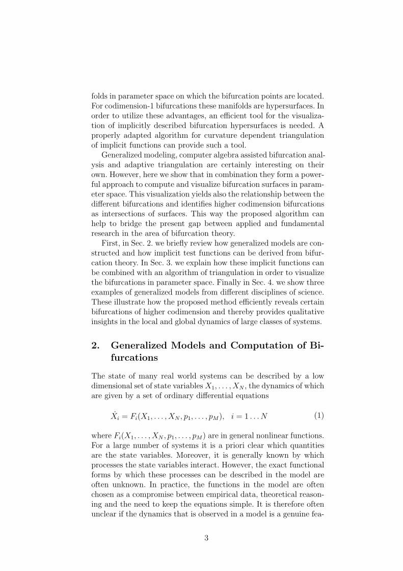
We construct an interim triangle by mirroring p1 at the straightline through p2 and p3 and to find a point p4 initial on the surfaceas shown in Fig.1. Thus p4 initial defines together with p2 and p3

the interim triangle. The angle φ between the normals of the new

7

triangle and the parent is used to approximate the local radius ofcurvature. Following Karkanis & Stewart [2001] we define the radiusof curvature as

R =d

2sin(

φ2

) (14)

where d the distance of the centers of both triangles (cf. Fig. 1).We choose a desired ratio ρ = R/d to compute a curvature adapteddistance dadapt = R/ρ. Finally we use again the Newton-Raphsonmethod to find a bifurcation point p4 at the distance dadapt fromthe straight line through p2 and p3 in the direction of p4 initial. Thebifurcation points p2,p3 and p4 then are the vertices of the adaptedtriangle. As mentioned above the adjacent triangles have to satisfyadditional requirements. In order to maintain a minimal resolutionwe define a maximum dmax. To restrict the number of computedbifurcation points we also define a minimum dmin. If dadapt is largerthan dmax or smaller than dmin we set it to dmax or dmin respectivelyto find p4. To check the quality of the adapted triangle we alsodefine a maximum angel φmax. We decrease the distance d, if theangle between the normals of the triangles is greater than φmax .

Proceeding as described above the algorithm adds to every tri-angle up to two adjacent triangles. In order to prevent overlappingtriangles, we reject a triangle if its center is closer to the center of anopposite triangle than one and a half times the largest edge of both.To allow for self intersections of bifurcation surfaces (s. Sec.4.3.), weallow an intersection of triangles if the angle between the normalsof the triangles is bigger than 2φmax. Another possibility which hasto be taken into account is that our system may possess more thanone bifurcation surface. To prevent transitions φmax has to be smallenough. For instance, if two surfaces intersect at an angle φ, we haveto choose φmax much smaller than φ. Concerning Hopf bifurcationsthe Hopf number χ offers a tool to distinguish between different sur-faces, even if the angle of intersection is very small. Along one Hopfbifurcation surface χ varies smoothly. On a different Hopf bifurca-tion surface the Hopf number is in general different since anotherpair of purely imaginary eigenvalues is involved. We can thereforecheck the continuity of χ between the new bifurcation point and theparent to make sure that the new point belongs to the same surface.

Since the bifurcation surfaces are in general not closed, we haveto restrict the parameter space according to a volume of interest V .We choose minimal and maximal values for each variable to definea cuboid which includes V . Triangles with vertices outside of thecuboid are rejected.

8

Apart from this restriction it is possible, that we find borders ofthe bifurcation surface within our cuboid. One example is a Hopfbifurcation surface that ends in a Takens-Bogdanov bifurcation asdescribed in Sec.2. If we cross the Takens-Bogdanov bifurcation,the new point still can be settled down on the surface described bythe test function. But in this case the Hopf number χ is positiveand the symmetry condition is satisfied by a pair of purely realeigenvalues that is not related to a bifurcation situation. To place thenew point directly onto the border of the Hopf bifurcation surface wecompute the root of the χ-function using the coordinates of the newpoint as initial conditions. Then we use the resulting point againto find the root of our test function. Repeating this procedure wefind iteratively our new point directly on the border of the Hopfbifurcation surface. In this way we can not only prevent a jumpfrom one Hopf bifurcation surface to another one by checking thesign of χ, but we also approximate the border of the Hopf bifurcationsurface.

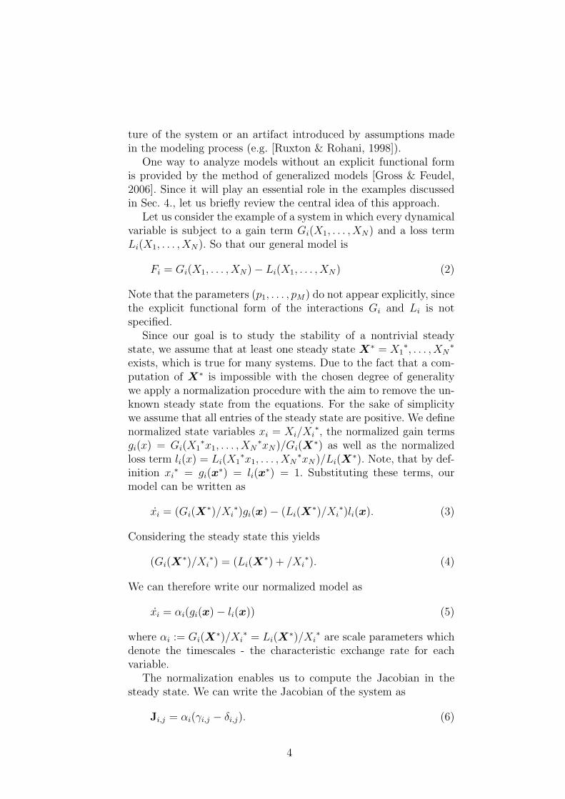
Following the procedure described above we can successively addtriangles to our mesh until no further triangle is possible. Afterthe growing phase the complete surface, in the prescribed region ofparameter space, is covered by a mesh of triangles as seen in theupper diagram in Fig.2.

3.4. Focus

Sometimes the bifurcation surfaces are quite smooth but in someregions they possess a more complicated structure. If the radiusof curvature changes too rapidly the algorithm fails to adapt thesize of the triangles and the structure is poorly approximated inthis region. In these regions it is useful to increase the minimalresolution in order to obtain a more accurate approximation of thebifurcation surface. We realize this by so-called focus points. In acertain radius r around these focus points we reduse the maximalsize of the triangles. The new maximal triangle size ˆdmax is thengiven as

ˆdmax =

(c + (1−c)r

r

)dmax r < r

dmax r ≥ r, (15)

where r is the distance to the closest focus point and c is a constantbetween 0 and 1. By definition ˆdmax decreases linearly with r fromdmax to a lower value cdmax, where c is a constant between 0 and 1.In Fig. 2 we see a triangulation of an example surface after the grow-ing phase. The upper diagram shows that two centers of a higher

9

resolution exit. The lower diagram shows that the surface looks likea landscape with a hill and a plane. One center of high resolutionis on top of the hill and the other one in the plane. This exampleshows both resolution control mechanisms, the size adaption due tothe radius of curvature (left) and due to a focus point (right).

While in Fig. 2 the focus point is not advantageous, this addi-tional resolution control is essential for the computation of rathercomplicated bifurcation situations (s. Sec.4.).

3.5. Filling phase

While the growing phase covers a large fraction of the surface withconnected traces of triangles, space between the traces remain. Whilewe fill this gap, we have to take care that we do not fill space that liesoutside the bifurcation surface, e.g. beyond a Takens-Bogdanov bi-furcation. In the following we start by describing the filling phase forsurfaces without boundaries and then go on to explain how bound-aries are handled.

The first task we have to perform in the filling phase is to identifythe gap. We can acquire the gap between the traces by starting ata vertex p1 and following the vertices at the boundary clockwise. Inthis way we construct a sequence of all N vertices.

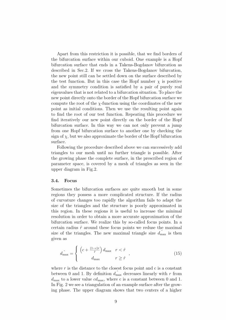
Once we have defined a gap we start to separate the gap intosubgaps. To each point of the gap we associate the normal nk of anadjacent triangle and the closest neighbor. Similar to Karkanis &Stewart [2001] we define all points as neighbors of pk which are lo-cated between the two half planes which are spanned by the normalnk and the two vectors from pk to pk−1 and pk+1 shown in Fig. 3(a).The closest neighbor of pk is the neighbor with the smallest Euclid-ian distance. If we find two points, which are the closest neighborsto each other they form a so-called bridge. We divide the gap at thefirst bridge we find into two subgaps by connecting the two vertices.If a subgap consists of only three vertices, we add it as a triangle tothe mesh we obtained from the growing phase. We proceed with thesubgaps as described above until no bridges are left. Afterwards wedivide the remaining subgaps at the point with the smallest distanceto its closest neighbor. In the end of this procedure the hole gap iscompletely filled up with triangles.

3.6. Borders in the filling phase

If the bifurcation surfaces are not closed but possess some bound-aries due to margins of the parameter region under consideration,or due to a codimension-2 bifurcation e.g. a Takens Bogdanov bi-

10

furcation then we have gaps which are not supposed to be filled up.In order to prevent bridges connecting these borders, we use similarcriteria for the bridges and all connections we make to divide thegaps, as used in the growing phase.

First, the connections the algorithm produces by the division ofgaps should not be much larger than dmax to preserve a minimalresolution. In order to prevent long connections at the margins ofthe parameter region we look for closest neighbors in a radius of3dmax. In order to prevent triangles with edges longer than 2dmax,we choose the maximal connection length as 1.8dmax. If a connectionis longer, we compute an additional point on the surface close to themiddle of the bridge and take this additional point into account.This criterion may also prevent the filling of an area where the bi-furcation condition is not satisfied. This is particularly true in caseof a Hopf bifurcation if the Hopf number χ is positive at this point.As described above the algorithm would automatically try to finda bifurcation point at the border of the Hopf bifurcation surface.If the computation of the new bifurcation point fails the division isdenied.

Second, the angles between the resulting triangles and the tri-angles of the mesh should not be larger than φmax. This criterionkeeps the triangulation smooth and may prevent the covering of amore complex region of the surface. Let φi and φj denote the anglesbetween the connection and the normals ni and nj associated tothe connected vertices as shown in Fig.3(b). Further, we denote φn

as the angle between the two normals ni and nj (see Fig.3(c)). Ifthe difference from φi and φj to 90 degrees is larger than φmax orφn is larger than φmax, we compute an additional point between aswell. As illustrated in Fig.3(d) a new point in the connection willin general cause a kink. If the angle of the kink in the connection isbigger than φmax, the division is denied. If we can not compute thenew point, because probably the bifurcation does not exist close toit, the division is also rejected.

Having obtained an adaptive triangulation of the bifurcation sur-face, we have to consider how to display the set of triangles.

3.7. Level lines

One the one hand visualization of the edges of the triangles can leadto visual fallacies. Small triangles seem to be far away while largetriangles may look very close. Focus points sometimes exacerbatethis effect. On the other hand not displaying only the triangle sur-face without edges would deprive the viewer of clues on the threedimensional shape of the surface. We introduce level lines as a cos-

11

metic tool. Like the level lines in a map we project certain valuesfrom the axes onto the surface.

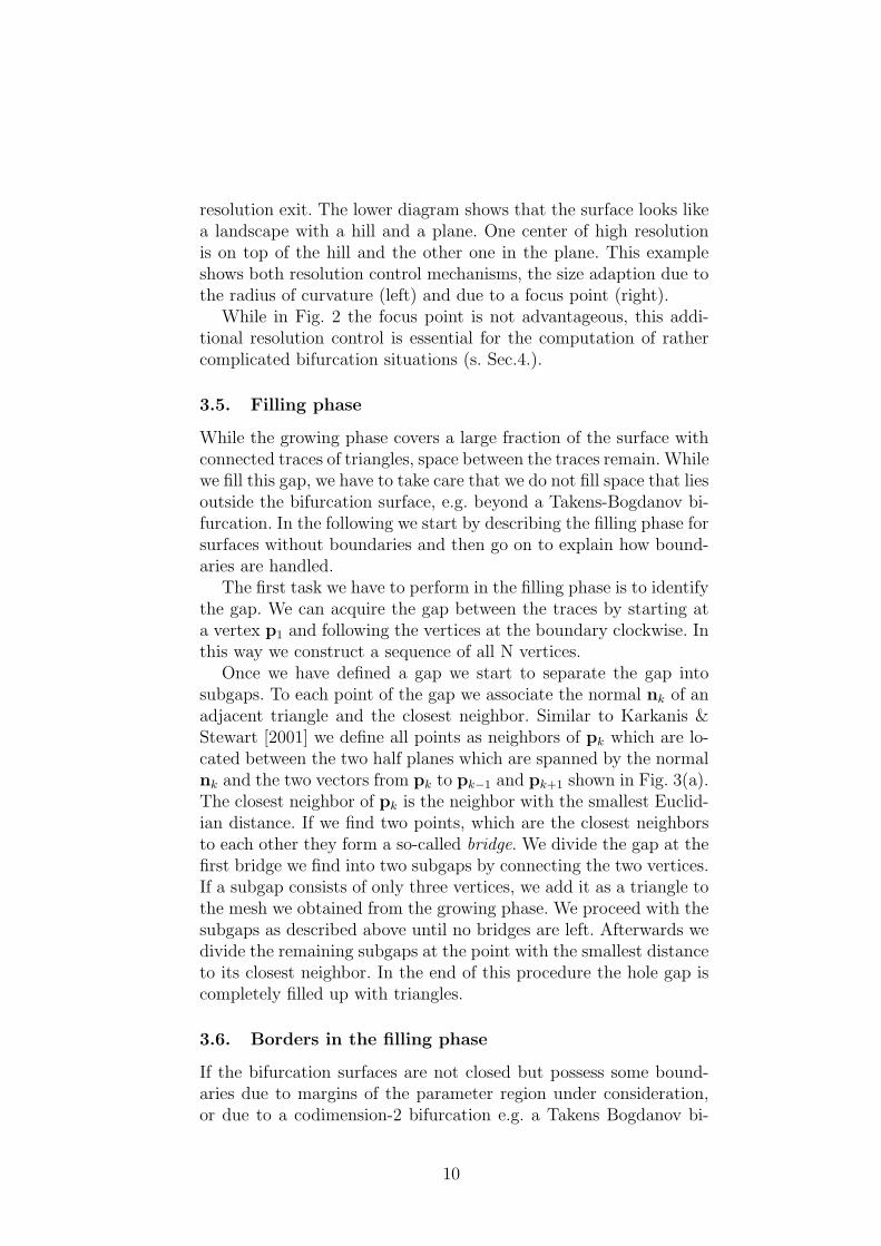
Finally we demonstrate the ability of our algorithm by the com-putation of a Whitney umbrella type bifurcation surface which mayappear as a higher codimension bifurcation for Hopf bifurcations(cf. Sec.4.3.). In this case the bifurcation surface is twisted in itself(cf. Fig.4). Even close to the end of the intersection line, where thecrossing angle becomes small, no transitions occur. While in mostregions the degree of curvature is quite small, a sharp edge appearsclose to the end of the line where the Hopf bifurcation intersectsitself. Since the radius of curvature decreases rapidly at this edgefrom a quite high value to a very small one, the adaptive resolutioncontrol would fail to adapt the size of the triangles in this region.However, using focus points close to the end of the crossing line wecan prevent bigger gaps in this region.

After the filling phase is completed (Fig. 4(b)) we cut off theouter triangles in order to obtain even margins at the boundary ofthe region in parameter space. Instead of the triangles we displaynow the level lines on the surface for both horizontal axes in Fig.4(b). As mentioned above not only the bifurcation surfaces but alsothe intersection lines are of interest since they form bifurcationsof higher codimension. In order to highlight these bifurcations wefinally mark the intersection line and its endpoint as shown in Fig.4(d).

4. Examples

In order to demonstrate the wide applicability of our algorithm letus now consider three examples from different disciplines of science.We start with a socio-economic model and continue with a metabolicnetwork as well as a food chain model from population dynamics

4.1. Bifurcation analysis of a generalized socio-economicmodel

While the history of China is characterized by periodic transitionsbetween despotism and anarchy the European dynasties exhibit sta-ble behavior for extended periods of time. A simple model describingthe interaction of three different parts of the society, namely farmersX1, bandits X2 and rulers X3 can predict such dynastic cycles aswell as steady state behavior. The specific model has been investi-gated in Feichtinger et al. [1996], Gross & Feudel [2006] studied ageneralized version of this model. The generalized model is given as

12

a system of three differential equations

X1 = S(X1)− C(X1, X2)− T (X1, X3),

X2 = ηC(X1, X2)− L(X2, X3)−M(X2),

X3 = νC(X1, X2)−R(X3),

(16)

where η and ν are constant factors.For the sake of clearness we refer to the individual processes by

different letters and not by different indices as we have done inSec.2. The function S(X1) denotes the gain or growth terms of thefarmers which already includes natural mortality. The loss termsC(X1, X2) and T (X1, X3) which reduce the population of farmersrepresent crime and taxes respectively. Because the population ofbandits benefits from crime the function C(X1, X2) multiplied witha constant factor η which denotes the gain term of the bandits. Therulers benefit from crime as well, because crime increases the will-ingness of farmers to support the rulers. Therefore, the number ofrulers grows also proportional to C(X1, X2) with a constant factorν. The rulers reduce the number of bandits by fighting crime. Thiseffect is taken into account by the term L(X2, X3). Finally the mor-tality of the bandits and the rulers is expressed by the terms M(X2)and R(X3) separately.

The normalization procedure from Sec. 2. that leads to the scal-ing and generalized parameters is shown in detail in [Gross & Feudel,2006]. Here we focus on the computation ond visalization of the bi-furcaation surfaces in order to illustrate the advantages of the pro-posed method. The steady state can undergo saddle-node and Hopfbifurcations (Fig. 5). The considered parameter space is spanned by3 parameters. The first parameter β1 (βx in [Gross & Feudel, 2006])is a scaling parameter of the normalized model. It is the ratio offarmer losses due to crime and the total farmer losses in the steadystate. It tends to one if the losses of farmers due to crime is muchlager than the losses due to taxes. The parameters s1 and c2 (sx andcy in [Gross & Feudel, 2006]) are so called generalized parameters.They appear in the Jacobian of the normalized model as the deriva-tives of the normalized processes in the steady state like γi,j and δi,j

in Sec. 2.. In that sense they are a measure of the nonlinearity ofthe corresponding process. As it has been noted they can be inter-preted in the context of the model under consideration. For instances1 corresponds to λ1,1 in Sec. 2. and is defined as the derivative ofthe normalized term s(x1) = S(X1

∗x1)/S(X1∗) with respect to x1

in the steady state. However, we can take it as a measure of avail-able land. If there is plenty of usable land available, the productivity

13

Term S(X1) is expected to be proportional to the number of farm-ers X1. In this case the parameter s1 is one. By contrast, if thereis a shortage of usable land s1 approaches zero. In a similar way,the derivative c2 of the normalized term c(x1, x2) with respect tox1 may symbolize the autonomy of the bandits in the steady state.If the bandits do neither constrain each other nor cooperate c2 isequal to one. While in case of competition between the bandits c2 isexpected to be smaller than one. These interpretations allow us toobtain a qualitative understanding of the results of our bifurcationanalysis.

The red surface in Fig. 5 is a manifold of Hopf bifurcation pointsand the slightly transparent blue surface is a manifold of bifurcationpoints of saddle-node type. The steady state is stable in the top-mostvolume on the right side of the parameter space and unstable every-where else in the diagram. Starting from any point within the stablevolume an increase of β1 causes the crossing of the Hopf surface ata certain value. At this point the stability is lost and a limit cycleoccurs. This transition can be understood as a change from a sta-ble dynasty to dynastic cycles. In that sense the parameter β1 andtherefore a domination of crime in farmer losses tends to destabilizethe system.

While the shape of the surfaces helps to understand the (de-)stabilizing effects of the bifurcation parameters, the intersectionsof these surfaces (dashed lines) give informations about other bifur-cations to be expected in the system and about the global dynamicsof the system. Our diagram contains two such lines. The almostvertical dashed line marks a Takens-Bogdanov bifurcation (TB) linewhich is characterized by two zero eigenvalues. As we know fromSec. 2., at least one homoclinic bifurcation has to emerge from theTakens-Bogdanov bifurcation. The horizontal dashed line marks across section of the surface of Hopf bifurcations and the surface ofgeneralized saddle-node bifurcations, where we find a zero eigenvaluein addition to a purely imaginary pair of complex conjugate eigen-values. This codimension-2 bifurcation is a Gavrilov-Guckenheimer(GG) bifurcation [Gavrilov, 1980, Guckenheimer, 1981] which arisesfrom a so called triple-point bifurcation with a triple zero eigenvalue.A homoclinic bifurcation emerges from the Gavrilov-Guckenheimerbifurcation as well. In addition, a Neimark-Sacker bifurcation whichis related to the emergence of quasiperiodic motion can be found.Due to these additional bifurcations in the neighborhood of theGavrilov-Guckenheimer bifurcation, parameter regions of quasiperi-odic dynamics exist and chaos is likely to occur. As Fig. 5 showsthese regions are expected to occur at moderate values of s1 andat relatively high values of β1. By contrast, at low values of β1 no

14

such regions can be found. Thus we can conclude that a dominationof crime in farmer losses tends not only to destabilize the systemlocally but may also lead to quasiperiodic and chaotic dynamics.

4.2. Bifurcation Analysis of a Model of Intracellular Cal-cium Oscillations

Similar to the socio-economic system considered above, the funda-mental biochemical processes that take place in living cells cannotbe understood without recourse to mathematical modeling. Thusrecently the concept of generalized models was extended to incor-porate the specific structural properties of cellular metabolism todescribe and elucidate the possible dynamics of metabolic and bio-chemical systems [Steuer et al., 2006].To exemplify the computation and visualization of bifurcation sur-faces in generalized models of cellular regulation, we consider aminimal model of intracellular calcium oscillations. Though strictlyspeaking not a genuine metabolic system, calcium ions (Ca2+) arean ubiquitous intracellular messenger and are involved in the reg-ulation and control of numerous cellular processes [Berridge et al.,2000]. Periodic temporal variation in the intracellular concentrationof calcium is known for a long time and is observed in a large varietyof different cell types [Berridge et al., 2000, Schuster et al., 2002].Furthermore, due to the universality and the importance in intracel-lular signaling, the analysis of calcium oscillations has been accom-panied by mathematical modeling almost from the beginning [Schus-ter et al., 2002]. In particular the observation of more complex formsof self-sustained calcium oscillation, such as bursting and chaotictemporal behavior, triggered an eminent interest in the analysis ofthe local and global bifurcations that arise in minimal and moreelaborate models of intracellular calcium dynamics [Schuster et al.,2002].Following a previously proposed model of calcium dynamics [Houartet al., 1999, Goldbeter et al., 2001], consisting of 3 concentrationvariables and 6 reaction and transport fluxes, we restrict our analy-sis to the key processes depicted in Fig. 6: Cells mobilize cytoplasmicCa2+ from internal, as well as external sources. Internal stores areheld within various intracellular compartments, most dominantelythe endoplasmatic reticulum (ER). Release of Ca2+ is controlled byinositol 1,4,5-triphosphate (InsP3), as well as by the cytoplasmicCa2+ concentration itself (calcium-induced calcium release, CICR).Given the model structure depicted in Fig. 6, the system can berepresented by a set of 3 differential equations, corresponding to thetime dependent concentrations of cytoplasmic calcium Ca2+

cyt (X1),

15

available calcium in the store Ca2+store (X2), and cytoplasmic inosi-

tol 1,4,5-triphosphate (X3). The respective differential equations arethen defined by the product of the 3× 6 dimensional stoichiometricmatrix N and the (as yet unspecified) 3-dimensional vector of rateequations K(X), describing the dependence of the reaction ratesand transport processes on the respective concentrations.

d

dt

X1

X2

X3

= NK(X) =

+1 −1 +1 −1 0 0

0 0 +1 −1 0 0

0 0 0 0 +1 −1

K1

K2(X1)

K3(X1, X2, X3)

K4(X1)

K5

K6(X1, X3)

(17)

Using the generalized approach described previously [Steuer et al.,2006], the information contained in Eq. (17) is already sufficient tofully specify a parametric representation of the Jacobian matrix ofthe normalized system.

Jx := Λθµx =

α1 −α1 +α2 −α2 0 0

0 0 +α3 −α3 0 0

0 0 0 0 +α4 −α4

·

0 0 0

θ21 0 0

θ31 θ3

2 θ33

θ41 0 0

0 0 0

θ61 0 θ6

3

(18)

In this parametric representation of the Jacobian, the elements ofthe 3 × 6 dimensional matrix Λ correspond the (inverse) charac-teristic timescales of the reaction and transport processes and arefully specified by the stoichiometry of the system and the (often ex-perimentally accessible) steady state concentrations X∗ and steadystate flux values K∗ = K(X∗).

α1 :=K∗

1

X∗1

α2 :=K∗

3

X∗1

α3 :=K∗

3

X∗2

α4 :=K∗

5

X∗3

(19)

The elements of the 6× 3 dimensional matrix θµx are defined as the

partial derivatives of the (normalized) rate functions with respect

16

to the (normalized) concentration variables at the steady state X∗.

θji :=

∂kj(x)

∂xi

∣∣∣∣∣x∗=1

with kj :=Kj(X)

Kj(X∗)and xi :=

Xi

X∗i

(20)

As demonstrated previously [Steuer et al., 2006], each element θji

measures the normalized degree of saturation of a reaction Kj withrespect to a metabolite Xi at the steady state X∗ and can be as-signed to a well-defined interval, even when the explicit functionalform of the respective rate equation is not known. For example, ex-port of calcium to the extracellular medium, as described by thetransport reaction K2(X1), depends only on cytoplasmic calciumconcentration Ca2+

cyt (X1). The second row in θµx thus only contains

a single positive nonzero entry in the first column θ21 ∈ [0, 1], cor-

responding to the (normalized) saturation of the export reactionK2(X1) with respect to its substrate X1. Similar, release of Ca2+

from the internal store by the transport reaction K3(X) dependson the available calcium in the store X2, thus θ3

2 > 0. Additionallythe export reaction K3 is activated by cytoplasmic calcium Ca2+

cyt

(X1) and InsP3 (X3), thus the respective saturation parameters areθ31 ∈ [0, n] and θ3

3 ∈ [0, n], where n denotes a positive integer de-scribing the cooperativity of the reaction.Equation (18), together with its interpretation in biochemical terms,now allows for a systematic analysis of the characteristic bifurcationsof the Jacobian matrix, without the need to specify the explicit func-tional form of any of the involved rate equations [Steuer et al., 2006].Figure 7 depicts a bifurcation diagram of the model as a function of3 generalized saturation parameters. As in the previous sections, thered surface displays a manifold of Hopf bifurcations and the slightlytransparent blue surfaces are manifolds of generalized saddle-nodebifurcations. Similar to the first example, the steady state is sta-ble in the top right volume of the diagram. If we cross one of thesurfaces the stability is lost. For this reason, increasing the satu-ration of calcium release with respect to cytoplasmic calcium, thusdecreasing the saturation parameter θ3

1, inevitably leads to a loss ofstability. If the value of θ3

2 is low, this loss of stability is related toa Hopf bifurcation. This means that either an unstable limit cyclevanishes or a stable limit cycle occurs. The latter case explains thecommonly observed calcium oscillations.However, as has been noted above, most interest today focuses onthe explanation of more complex dynamics. It has been shown thatspecial models of the form of Eq.(17) can account for complex in-tracellular Ca2+ oscillations [Borghans et al., 1997, Goldbeter et al.,2001, Houart et al., 1999]. The question is wether these dynamics

17

result only from the more or less arbitrary assumptions about theexact functional form of the rate equations K, or whether they re-sult from more elementary properties of the system, such as thestoichiometry and the assumed regulatory interactions. The advan-tage of the generalized model, and hence of our conclusions aboutpossible dynamics, is that these are independent from the former:The localization of bifurcations of higher codimension provides thedesired information on global dynamics, independent of the exactfunctional form of any of the involved rate equations. Figure 7 showsthat the Hopf bifurcation surface emerges from and ends in a Takens-Bogdanov bifurcation line. The two lines where this surface crossesthe generalized saddle-node bifurcation surfaces are Gavrilov Guck-enheimer bifurcation lines. Again, as described in Sec.4.1. this showsthe existence of quasiperiodic and chaotic parameter regions in themodel close to the GG lines. While in Fig. 7 the parameter θ3

3 onlyvaries within the range [0, 1] the model discussed by Houart et al.[1999] allows a maximum value of 4. However, the GG lines can befound in the whole range except for small values of θ3

3. Here, theGG lines vanish at the TB lines in triple point bifurcations. As avariety of global bifurcations is located in the neighborhood of thesetriple point bifurcations, we can expect the richest dynamics in thisregion.

4.3. Bifurcation analysis of a general food chain model

Our last example is a generalized four-trophic food chain model.Each trophic level n may correspond to one species or to a groupof similar species Xn. The first level X1 is called primary producerand the last level X4 is named top predator. A generalized modelof such food chains is given in Gross [2004] which can be written inthe four-trophical case as

X1 = S(X1)− F1(X1, X2),

X2 = η2F1(X1, X2)− F2(X2, X3),

X3 = η3F2(X2, X3)− F3(X3, X4),

X4 = η4F3(X3, X4)−M(X4),

(21)

where the term S(X1) denotes the primary production which isassumed to depend on X1 and M(X4) describes the mortality ofthe top predator. The biomass loss of species Xi due to predationby species Xi+1 is given as Fi(Xi, Xi+1) where i = 1..3 and ηi+1

describes the fraction of biomass predation that is converted intobiomass of the predator. While S(X1) could also include natural

18

mortality of the primary producer (apart from predation) we as-sume that predation is much higher than natural mortality. As aresult we neglect the natural mortality of species X2 and X3. Ac-cording to the procedure described in Subsection 2. the normalizedmodel of (21) can be written as

x1 α1(s(x1)− f1(x1, x2)),

x2 = α2(f1(x1, x2)− f2(x2, x3)),

x3 = α3(f2(x2, x3)− f3(x3, x4)),

x4 = α4(f3(x3, x4)−m(x4)),

(22)

where we can identify αn, n = 1 . . . 4 again as inverse timescaleparameters. Following Gross et al. [2004] we assume an allometricslowdown of the timescales described by the ratio r = αn+1/αn < 1.Applying a normalization of time we can set α1 = 1 and αn = rn−1.Thereby we express all scaling parameters by the parameter r thatdescribes the timescale separation. Another bifurcation parameterwe use is the sensitivity to prey γn := ∂fn(xn, xn+1)/∂xn, n = 1 . . . 3.If prey xn is abundant the parameter γn will approach zero. It islarger if prey is scarce and equal to one if predation is proportionalto prey density. As Gross [2004] pointed out, the value of γn dependsstrongly on the feeding strategy of predator xn+1.

In the four-trophic food chain the steady state loses its stabilityin a Hopf bifurcation. As shown in Fig. 8 the surface of Hopf bifur-cations possesses a rather complicated shape. It turns out that thefour trophic food chain is one of the rare examples of applicationsthat exhibits a Whitney umbrella type bifurcation, used in Sec. 3.to illustrate the capabilities of the algorithm presented. It is formedaround a codimension-3 1:1 resonant double Hopf bifurcation at theend of the line of double Hopf bifurcations (DH) of codimension 2. Ithas been shown that chaotic parameter regions generally exist closeto a double Hopf bifurcation [Kuznetsov, 1998].

The parameter range in which the 1:1-resonant double Hopf bi-furcation occurs can only be reached if the predation rates can be de-scribed by Holling type-III predator-prey interaction [Holling, 1959].However, such interactions are frequently observed in nature. To ourknowledge, this is the first example of a 1:1-resonant double Hopfbifurcation that was found in an applied model. Moreover, the ex-istence of the bifurcation in the generalized model shows that thisbifurcation can generically be found in a large class of four throphicfood chains. Generalized models of longer food chains and morecomplex food webs often exibit multiple 1:1-resonant double Hopf

19

bifurcations.

5. Discussion

In this paper we have proposed and applied a combination of gener-alized modeling, bifurcation theory and adaptive triangulation tech-niques. This approach has enabled us to compute and visualize thelocal codimension-1 bifurcation hypersurfaces of steady states. Inorder to obtain a faithful representation of the surface at a low com-putational cost the algorithm automatically adapts the size of thecomputed triangle elements to the local complexity of the surface.Due to the application of generalized modeling, the resulting bifur-cation diagrams do not describe a single model, but a class of modelsthat share a similar structure.

The proposed approach enables the researcher to rapidly computethree parameter bifurcation diagrams for a given class of models. Byconsidering several of these diagrams with different parameter axesan intuitive understanding of the local dynamics in a given classof systems can be gained. In particular, the approach bridges thegap between applied and fundamental research as discussed in theIntroduction. In the visualization of local bifurcations as surfacesin a three dimensional parameter space, certain local bifurcations ofhigher codimension can be easily spotted. In our experience the pro-posed approach reveals bifurcations of codimension two and three inalmost every model studied. It thereby provides plentiful examplesfor mathematical analysis. In return insights gained from the inves-tigation of higher-codimension bifurcations can directly feed backin the investigation of the system. In particular the implicationsof local bifurcations of higher codimension, discussed above, is in-triguing in this context. Provided that the dynamical implicationsof a bifurcation are known from normal form theory, the appearanceof such a bifurcation in the three parameter diagram, pinpoints aparameter region of interesting dynamics. This region can then beinvestigated in conventional models or experiments. In this way theinvestigation of models is facilitated by reducing the need for morecostly parameter search in conventional models.

In the present paper we have only used the proposed approachin conjunctions with testfunctions for two basic local bifurcations:the Hopf bifurcation and the saddle-node bifurcation. However, inprinciple, the approach can be extended to include testfunctionsfor codimension-2 bifurcations. This would allow the algorithm toadaptively decrease the size of triangles close to these bifurcationsand continue the bifurcation lines directly once they are reached.

20

Furthermore, being hyperlines, the codimension-2 bifurcation pointsform surfaces in a four dimensional parameter space. Once againthese surfaces can be triangulated with the described algorithms.The four dimensional space could be visualized in a movie, wheretime represents the forth parameter or by collapsing and color codingone of the parameter dimensions. Both approaches would allow forthe visual identification of bifurcations of codimension three andhigher.

At present the proposed approach has two limitations. First, theextraction of information is solely based on the Jacobian. Higherorders, which determine the normal form coefficients, are at presentnot taken into account. However, parameters that capture this in-formation could be defined in analogy to the exponent parameters,which we have used to capture the required information on the non-linearity of the equations of motion.

The second limitation is that the approach outlined here is presentlyonly applicable to systems of small or intermediate dimension (N <10) as the analytical computation of the testfunctions becomes cum-bersome for larger systems. This problem can be avoided by combin-ing the triangulation techniques proposed here with the numericalinvestigation of generalized models demonstrated in [Steuer et al.,2006].

References

Agladze, K. I. & Krinsky, V. I. [1982] “Multi-armed vortices in anactive chemical medium,” Nature 296, 424 – 426.

Berridge, M. J., Lipp, P. & Bootman, M. D. [2000] “The versalityand universality of calcium signalling,” Nature Reviews MolecularCell Biology 1, 11–12.

Borghans, J. A. M., Dupont, G. & Goldbeter, A. [1997] “Com-plex intracellular calcium oscillations: A theoretical explorationof possible mechanisms,” Biophysical Chemistry 66, 25–41.

Dijkstra, H. A. [2005] Nonlinear Physical Oceanography, 2nd ed.,vol. 28 of Atmospheric and Oceanographic Sciences Library.(Springer-Verlag, Berlin, Heidelberg, New York).

Feichtinger, G., Forst, C. V. & Piccardi [1996] “A nonlinear dynam-ical model for the dynastic cycle,” Chaos Solutions & Fractals 7,no. 2, 257–271.

Gavrilov, N. [1980] “On some bifurcations of an equilibrium withtwo pairs of pure imaginary roots,” in Methods of Qualitative

21

Theory of Differential Equations (GGU, USSR), pp. 17–30. inrussian.

Gelfand, I. M., Kaprov, M. M. & Zelevinsky, A. V. [1994]Discriminants, Resultants and Multidimensional Determinants.(Birkhauser, Boston).

Goldbeter, A., Gonze, D., Houart, G., Leloup, J.-C., Halloy, J. &Dupont, G. [2001] “From simple to complex oscillatory behaviorin metabolic and genetic control networks,” Chaos 11, no. 1,247–260.

Gross, T. [2004] Population Dynamics: General Results from LocalAnalysis. (Der Andere Verlag, Tonningen, Germany).

Gross, T., Ebenhoh, W. & Feudel, U. [2004] “Enrichment andfoodchain stability: the impact of different forms of predator-preyinteraction,” Journal of Theoretical Biology 227, 349–358.

Gross, T. & Feudel, U. [2004] “Analytical search for bifurcationsurfaces in parameter space,” Physica D 195, no. 3-4, 292–302.

Gross, T. & Feudel, U. [2006] “Generalized models as a universalapproach to nonlinear dynamical systems,” Physical Review E73, no. 016205. (14 pages).

Guckenheimer, J. [1981] “On a codimension two bifurcation,” Lec-ture Notes in Mathematics 898, 99–142.

Guckenheimer, J. & Holmes, P. [1983] Nonlinear Oscillations, Dy-namical Systems, and Bifurcations of Vector Fields, 1st ed., vol. 42of Applied Mathematical Siences. (Springer-Verlag, Berlin, Heidel-berg, New York).

Guckenheimer, J., Myers, M. & Sturmfels, B. [1997] “ComputingHopf bifurcations I,” SIAM J. Numer. Anal. 34, no. 1, 1.

Holling, C. S. [1959] “Some characteristics of simple types of preda-tion and parasitism,” The Canadian Entomologist 91, 385–389.

Houart, G., Dupont, G. & Goldbeter, A. [1999] “Bursting, chaosand birhythmicity originating from self-modulation of the inos-titol 1,4,5-triphosphate signal in a model for intracellular Ca2+

oscillations,” Bull. of Math. Biol. 61, 507–530.

Karkanis, T. & Stewart, A. J. [2001] “Curvature-dependent tri-angulation of implicit surfaces,” IEEE Computer Graphics andApplications 22, no. 2, 60–69.

22

Kelley, C. T. [2003] Solving Nonlinear Equations with Newton’sMethod (Fundamentals of Algorithms). (SIAM, Philadelphia).

Kuznetsov, Y. A. [1998] Elements of Applied Bifurcation Theory,2nd ed., vol. 112 of Applied Mathematical Siences. (Springer-Verlag, Berlin, Heidelberg, New York).

Ruxton, G. D. & Rohani, P. [1998] “Population floors and per-sistance of chaos in population models,” Theoretical PopulationBiology 53, 75–183.

Schuster, S., Mahrl, M. & Hofer, T. [2002] “Modelling of simpleand complex calcium oscillations: From single-cell responses tointercellular signalling,” Eur. J. Biochem. 269, 1333–1355.

Seydel, R. [1991] “On detecting stationary bifurcations,” Interna-tional Journal of Bifurcation and Chaos 1, no. 2, 335–337.

Steuer, R., Gross, T., Selbig, J. & Blasius, B. [2006] “Structural ki-netic modeling of metabolic networks,” Proc Natl Acad Sci U S A103, no. 32, 11868–11873.

Swinney, H. L. & Busse, F. H. [1981] Hydrodynamic instabilities andthe transition to turbulence. (Springer-Verlag, Berlin, Heidelberg,New York).

Titz, S., Kuhlbrodt, T. & Feudel, U. [2002] “Homoclinic bifurca-tion in an ocean circulation box model,” International Journal ofBifurcation and Chaos 12, no. 4, 869–875.

Zaikin, A. N. & Zhabotinsky, A. M. [1970] “Concentration wavepropagation in two-dimensional liquid-phase self-oscillating sys-tem,” Nature 225, 535 – 537.

23

Figure 1: Seed triangle with one adjacent triangle.

24

Figure 2: Example surface after the growing phase computed withone focus point. The size of the triangles adapts to the local curva-ture and the proximity to the focus point.

25

(a) The space of possible neighborsof pk is within the two half planesspanned by the normal nk associatedto pk and the two vectors from pk topk−1 and pk+1.

(b) The difference between the anglesφi and φj to 90 degrees has to be lessthan φmax

(c) The angle φn between the normalsof the connected points has to be lessthan φmax

(d) If an additional point in the mid-dle of the bridge is necessary the angleφkink has to be less then φmax

Figure 3: A connection in the filling phase is called bridge and hasto satisfy different conditions.

26

(a) The trace of triangles follows theevolution of the surface.

(b) Whitney umbrella surface after thefilling phase.

(c) Whitney umbrella surface after thefilling phase with level lines (no high-lighting of the triangle edges).

(d) Marking of intersection line and itsendpoint

Figure 4: Construction of a bifurcation diagram that shows a Hopfbifurcation surface possessing the shape of a Whitney umbrella. Thisbifurcation is found in a population dynamical system given in Sec.4.3. While the upper subplots (a) and (b) show the two phases ofthe triangulation algorithm, the lower subplots (c) and (d) illustratethe preparation of the resulting diagram.

27

Figure 5: Bifurcation diagram of a generalized socio-economic modelof farmers, bandits and rulers. The parameter β1 is the fraction offarmer losses caused by crime. The other parameters s1 and c2 repre-senting the availability of usable land and the autonomy of the ban-dits respectively. The red surface is a manifold of Hopf bifurcationsand the slightly transparent blue surface is a manifold of saddle-node bifurcations. The stitched lines mark a Gavrilov-Guckenheimer(GG) and a Takens-Bogdanov (TB) bifurcation. The intersectionpoint of these lines is a triple point bifurcation.

28

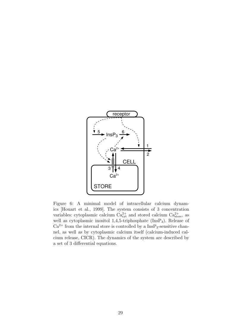
Figure 6: A minimal model of intracellular calcium dynam-ics [Houart et al., 1999]. The system consists of 3 concentrationvariables: cytoplasmic calcium Ca2+

cyt and stored calcium Ca2+store, as

well as cytoplasmic inositol 1,4,5-triphosphate (InsP3). Release ofCa2+ from the internal store is controlled by a InsP3-sensitive chan-nel, as well as by cytoplasmic calcium itself (calcium-induced cal-cium release, CICR). The dynamics of the system are described bya set of 3 differential equations.

29

Figure 7: Bifurcation diagram of a metabolic network model of cal-cium oscillations. The red surface is a manifold of Hopf Bifurca-tions and the slightly transparent blue surfaces are manifolds of gen-eral saddle-node bifurcations. The dashed lines denote a Gavrilov-Guckenheimer bifurcation (GG) and a Takens-Bogdanov (TB) bifur-cation. The intersection points of these lines are triple point bifurca-tions. Concentration and flux values, as well as all other saturationparameters are assumed to be constant, corresponding to the valuesfound in [Houart et al., 1999]: X∗

1 = 0.35, X∗2 = 0.9, X∗

3 = 0.13 (inarbitrary units) and θ2

1 = 0.15, θ61 = 0.25, θ6

3 = 0.8.

30

Figure 8: Bifurcation diagram of a four-trophic food chain. The valueof r describes the ratio between the characteristic timescale of apredator and its prey, while γ1,3 = γ1 = γ3 and γn describes thesensitivity of predator Xn+1 to its prey Xn. The red surface is amanifold of Hopf bifurcations that intersects with itself in a doubleHopf bifurcation line (DH) of codimension 2, which is shown asa dashed line. The end of this line is a 1:1 resonant double Hopfbifurcation (1:1 DH) of codimension 3.

31