Master's Degree Thesis ISRN: BTH-AMT-EX--2008/D-04--SE

Supervisors: Sharon Kao-Walter, Ph.D Mech Eng, BTH Junruo Chen, Professor, KUST, Kunming, China

Department of Mechanical Engineering Blekinge Institute of Technology

Karlskrona, Sweden

2008

Gao Feng Adelere Oluwafemi. A.

Computation and Analysis of Gas-Solid Flow Multiphysics

in a Pneumatic Dryer

Computation and Analysis of Gas-Solid Flow

Multiphysics in a Pneumatic Dryer

Gao Feng

Adelere Oluwafemi. A. Department of Mechanical Engineering Blekinge Institute of Technology

Karskrona, Sweden 2008 Thesis submitted for completion of Master of Science in Mechanical Engineering with emphasis on Structural Mechanics at the Department of Mechanical Engineering, Blekinge Institute of Technology, Karlskrona, Sweden.

Abstract: This work presents a design of drying small food particles like tea, tobacco with a reduced height of about fifty percent compared to the convectional straight type. The geometry is designed such that, the particle leave the dryer at an average constant time, to prevent variation in the dryness properties, Simulation result of straight type dryer in FLUENT, the commercial software is validated by industrial data implemented in MATLAB, which shows reasonable agreement. A reduced height type with a swirling or screw type is designed to reduce the height and also maintain the drying residence time. Keywords: Finite volume method ( FVM ) , SIMPLE method, Straight pipe dryer, Screw type dryer, MATLAB®, GAMBIT®, FLUENT®

2

Acknowledgements This work was carried out under the cooperation between the Department of Mechanical Engineering, Blekinge Institute of Technology and the Faculty of Electro-Mechanical Engineering, Kunming University of Science and Technology China under the supervision of Professor Junruo Chen and Dr. Sharon Kao-Walter We would like to express sincere gratitude to our supervisors Professor Junruo Chen and Dr.Sharon Kao-Walter, who made this collaborative research effort. The Lineaus-Palme International exchange between Blekinge Institute of Technology Sweden and Kunming University of Science and Technology China an incredible reality. We are also indebted to Mr. Xianxi Liu (PhD. student) for his valuable suggestions, and all members of staffs in Mechanical Engineering Departments of Blekinge Institute of Technology (BTH), Sweden and Kunming University of Science and Technology (KUST), China. For their guidance and professional engagement on the course of our study. Kunming, March 2008. Gao Feng. Adelere Oluwafemi. A.

3

Contents 1 Notation 7 2 Introduction 9 2.1 Background 9 2.2 Project Description 9 2.3Method 10 2.4 Limitation 10 3 Overview of Drying Process 11 3.1 Drying Process 12 3.2 Available Convective types 12 3.3 Existing Work 13 4 Theoretical Analysis 14 4.1 Derivations of Equations 14 5 Available Experimental Data 19 6 Numerical Analysis 20 6.1 Control-Volume Formulation (F V M) or (FEM) 20 6.2 The SIMPLE algorithm 21 6.3 Implementations Of Boundary Conditions 29 6.4 Drying In a Straight Pipe Model 30 6.5 Design and Working principle of the Swirling Dryer 32 7 Simulation 34 7.1 Choice of Commercial Softwear 34 7.2 Problem Formulation in Commercial Softwear 34 7.3 Boundary Condition 34 7.4 Assumptions 35 7.5 Postprocessing 35 8 Result And Analysis 36 8.1 Single Phase 36 8.2 Double Phase 40 8.3 Swirling type double phase 43 9 Conclusion and Future Work 46 9.1 Conclusion 46 9.2 Future Work 46 10 References 47 11 Appendices 49

A. Other Work In FLUENT 49 B. MATLAB Code 53

4

1 Notations

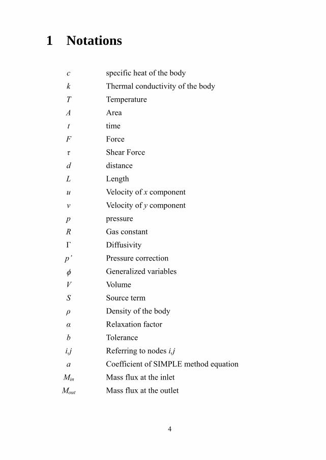
c specific heat of the body k Thermal conductivity of the body T Temperature A Area t time F Force τ Shear Force d distance L Length u Velocity of x component v Velocity of y component p pressure R Gas constant Г Diffusivity p’ Pressure correction

φ Generalized variables V Volume S Source term ρ Density of the body α Relaxation factor b Tolerance i,j Referring to nodes i,j a Coefficient of SIMPLE method equation

Min Mass flux at the inlet Mout Mass flux at the outlet

5

new New value after correction * Assumption value e East direction w West direction s South direction n North direction

6

2 Introduction

2.1 Background

Gas flow drying is an approach of convective desiccation. Hot gas convey the material to be dried into the drying equipment; As a result of the high temperature difference, convective heat transfer takes place between the hot gas and material during the transportation, thereby, removing moisture, inform of vapor from the material. The evaporated moisture from the product becomes part of the drying medium, and does not need to be exhausted, since the hot gas is superheated steam, unless the pressure increases beyond a set point, at which the excess steam may be released. This allows for the recycling of the drying medium, This approach is widely used in food, tobacco and some chemical, medical, fertilizer, dyestuff, inorganic compound, industry. Since the velocity of the airflow is quite high, the material granule is in suspending status, the contact area between the gas-solid two phases is large, so the heat transfer is intensified. The material drying time depends on the temperature of the hot gas, diffusibility of the material, initial and final moisture content. The temperature of the hot gas can adjust to control the temperature of the material and avoid quality change as result of overheating.

2.2 Project Description

However, it is not easy to design a proper drying system, factors mentioned earlier has to be taken into consideration. Such as the dryness quality, moisture content of the product. The disadvantages of the gas-flow drying; are the resistance of system flow is high and the effective distance of drying is rather long. The straight pipe type dry system commonly used for material drying is designed at a height of about 20 meters, which is too high to build the workshop. So ,the need to consider a new approach to lower the equipment height and also maintain the drying distance arise, with the design the screw type dryer system and make some numerical calculations to simulate the model for optimum design.

7

2.3 Method

Since the process of drying involves movement of particle from one point to another by hot gas, it is a mixture flow of solid (material) and gas (hot gas). There are research works on solid-gas, two-phase flows, and there are detail results, nevertheless, there are slight variations between the numerical simulation and the real situation due to the complexity and the limitation. An exploring investigation carried out in this paper is as follows:

• Finding the suitable mathematic model of coupled physic field; • Simplifying the model and making the reasonable assumptions; • Using numerical method to solve and implement in MATLAB; • Validating the results from MATLAB by commercial software; • Verifying the results from experimental test (optional);

Numerical simulation technology on the computer, to analysis the flow, and the heat transfer process in the project in question is an extremely economical and effective method, which save time and resources. The research results provided the theoretical basis for optimum product development and design, simultaneously, the method has provided useful means for the solid-gas two-phase flows research, but also built the foundation for the practical application.

2.4 Limitations

Effect of diffusibility, and porosity of the material media, compartment of the materials is not considered, only the drying residence time or drying time of the material is considered. Diffusion coefficient is a material property which is affected by the composition, shape, size of the product and process temperature. Also the mechanisms of separating the dry product from the superheated steam are not included in this work.

8

3 Overview of Drying Process

3.1 Drying Process

The primary objective of food drying is preservation of the product, and lowering the moisture content, which helps to prevent, or reduce microbial and enzymatic reactions; however, drying can have an adverse effect on chemical, physical, and nutritional value of food products [1]. Superheated steam is generally used gas for drying food substance to prevent contaminations as a result of chemical reactions; and the temperature is moderately high to prevent saturation of the drying gas and burning of the food particles as result of heat transfer. Goals of research is improving current drying technologies, and to improve on economics of operations ,that is reduce energy consumption, increase capacity, reduce size of equipment, increase ease of control, environmental considerations, reduce emissions, increase safety, and improve product quality, minimize chemical, physical, and nutritional degradation. Some of these goals must be proven to provide benefits that exceed additional costs and risks before industry is willing to adopt a new technology. [2] Drying is process of removing moisture from a material, this can be achieved or done by various methods and technologies, such as chemical decomposition of water in substance, that is, desiccants [3], which could be in form of absorption in gases and capillary action in solid [4].Compression, centrifugal and gravitational forces are employed as mechanical method of drying .Thermal drying is the most commonly used method in practical applications, it is an important means of reducing the moisture content of fruit, vegetables, and enhance resistance to degradation due to decrease in water activity. And the widely use type, is convective drying ,in which the gas temperature decrease as result of uptake of water from the material[5].Hot gases are made to flow over the surface of material to be dried and thermal energy is transferred from the hot gas to the material, by convection. The vapor as result of evaporation of the moisture is transported away by the air flow. In solids drying, there has often been a great difference between academic theory and industrial design practice. Traditionally, practical dryer design has tended to be base on simple correlations and scale-up from pilot-plant tests, rather than rigorous theoretical model [6]. However, drying processes involving solids are much more difficult to model than fluid-phase (liquid and gas) processes. Physical properties of

9

fluids can be obtained easily from databanks, and are uniquely defined for given temperatures and pressures, while the system is controlled by equilibrium thermodynamics. In contrast, physical properties of solids vary considerably with solids structure. For example, drying kinetics can differ by orders of magnitude for the same chemical substance depending on particle size, porosity, polymorph, etc. Drying is also inherently a non-equilibrium process; the moisture within a particle does not flash off instantly when exposed to hot dry air [7]. Drying of solid is generally understood to follow two distinct drying zones, namely the constant rate and the falling rate periods, with critical moisture content demarcating these zones. The constant rate period is understood to have maximum drying rate, which remain constant until the critical moisture content is reach. The extent of the drying zone is based on the type of the material. [8] However, the drying time of a particle depends on its initial moisture content, mass flow rate, temperature at inlet, bulk density, and final moisture content [9].

3.2 Available convective types

Fluidized bed can by classify as gas-solid transport system which are characterized by a continuous convective drying process very high particle resident time. The spouted bed type system for feeding solid into pneumatic transport tube provide a stable flow of particles, and offer operations of wide range of solid flow rate by changing air flow rate or the distance between the air inlet and the outlet in the tube transport ,unlike the normal feeder i.e. fluidized bed type[10]. Which is very important factor for product drying .Other types are fixed bed, pneumatic conveying, and impingement superheated steam dryer e.t.c

3.3 Existing work

Ferria et al [10] analyzed one dimensional fluid dynamic model based on continuity and momentum balance for dilute gas solid flow in a pneumatic dryer with a spouted bed type solid feeding system. And concluded that one –dimensional model does not provide a good description of the physical

10

phenomena and flow pattern involved in pneumatic vertical flow transport, due to inconsistence estimated value of solid-fluid interaction forces and slip velocities . More so, Somkiat et al [11] compared the performances of pulsed and conventional fluidized-bed dryers, based on consumption of energy, outlet moisture content, and quality of the dried. Experimental results have shown that the variation of moisture content at the exits of both dryer types in test runs was very small. Calculated thermal and electrical energy consumptions indicated that the pulsed flow dryer was more economical than the conventional dryer. Investigation of flow field and the heat transfer characteristics in a tangential inlet cyclone mainly used for the separation of the dens phase of a two phase flow Was carried out by Irfan and Fuat [12]. It was observed that heat transfer increases at all surfaces with the inlet velocity and decreases towards to cone apex. The maximum value of the Nusselt number occurs on the region opposite to the inlet section and this region displaces down slightly for high inlet velocities. Results obtained from their computer modeling have demonstrated that CFD is suitable for simulating the flow and heat transfer characteristics in cyclone separators.

11

4 Theoretical Analysis The solution of heat transfer, fluid flow, and other related processes can begin when the laws governing these processes have been expressed in mathematical form, generally in terms of differential equations. The governing equations of fluid flow represent mathematical statement of the conservation laws of physics. The statements are the following:

• The mass of a fluid is conserved. • The rate of change of momentum equals the sum of the forces on a

fluid particle, which is the Newton’s second law. • The rate of change of energy is equal to the sum of the rate of heat

addition to and the rate of work done on a fluid particle, which is the first law of thermodynamics.

4.1 Derivations and Descriptions Of Equations

4.1.1 Mass conservation equations

According to Versteeg H.K and Malalasekera. [17], any fluid flow problem must fulfill the mass conservation law. It is stated that the rate of the increase of mass in fluid element is equal to the net rate of flow of mass into fluid element. This yields the mass conservation equations:

( ) ( ) ( ) 0u v w

t x y zρ ρ ρ ρ∂ ∂ ∂ ∂+ + + =

∂ ∂ ∂ ∂ (4.1)

Or in more compact vector notation

( ) 0div utρ ρ∂+ =

∂ (4.2)

The equation (4.2) is unsteady, three-dimensional mass conservation or continuity equation at a point in a compressible fluid. The first term on the left hand side is the rate of change in time of the density (mass per unit volume). The second term describes the net flow of mass out of the element across its boundaries and is called the convective term.

4.1.2 Momentum conservation equations

Newton’s second law states that the rate of change of momentum of a fluid

12

particle equals the sum of the forces on the particle [17]. According to this law, one can derive the momentum conservation equations in x, y and z three directions：

( ) ( )

( ) ( )

( ) ( )

yxxx zxx

xy yy zyy

yzxz zzz

u pdiv uu Ft x x y zv pdiv vu F

t y x y zw pdiv wu Ft z x y z

ττ τρ ρ

τ τ τρ ρ

ττ τρ ρ

∂∂ ∂∂ ∂+ = − + + + +

∂ ∂ ∂ ∂ ∂∂ ∂ ∂∂ ∂

+ = − + + + +∂ ∂ ∂ ∂ ∂

∂∂ ∂∂ ∂+ = − + + + +

∂ ∂ ∂ ∂ ∂

(4.3)

Where p is the pressure on the fluid element; τxx, τxy and τxz etc. are the viscosity shear components on the fluid element due to the molecule viscosity. Fx, Fy and Fz are the body force of element. For Newtonian fluid, the viscosity stresses τ is proportional to the rate of deformation [17]. Thus:

2 ( )

2 ( )

2 ( )

xx

yy

zz

xy yy

xz zy

yz zy

u div uxv div uyu div uz

u vy xu wz x

v wz y

τ μ λ

τ μ λ

τ μ λ

τ τ μ

τ τ μ

τ τ μ

∂= +

∂∂

= +∂∂

= +∂

⎛ ⎞∂ ∂= = +⎜ ⎟∂ ∂⎝ ⎠

∂ ∂⎛ ⎞= = +⎜ ⎟∂ ∂⎝ ⎠⎛ ⎞∂ ∂

= = +⎜ ⎟∂ ∂⎝ ⎠

(4.4)

Where μ is dynamic viscosity, λ is the second viscosity. Substitute equation (4.4) into (4.3):

13

( ) ( ) ( )

( ) ( ) ( )

( ) ( ) ( )

u

v

w

u pdiv uu div grad u St xv pdiv vu div grad v S

t yw pdiv wu div grad w St z

ρ ρ μ

ρ ρ μ

ρ ρ μ

∂ ∂+ = − +

∂ ∂∂ ∂

+ = − +∂ ∂

∂ ∂+ = − +

∂ ∂

(4.5)

Where Su, Sv and Sw are the generalized source term。Su=Fx,+Sx, Su=Fy,+Sy, Su=Fz,+Sz, and the expressions of Sx, Sy and Sz is the following:

( )

( )

( )

x

y

z

u v wS div ux x y x z x x

u v wS div ux y y y z y y

u v wS div ux z y z z z z

μ μ μ λ

μ μ μ λ

μ μ μ λ

∂ ∂ ∂ ∂ ∂ ∂ ∂⎛ ⎞ ⎛ ⎞ ⎛ ⎞= + + +⎜ ⎟ ⎜ ⎟ ⎜ ⎟∂ ∂ ∂ ∂ ∂ ∂ ∂⎝ ⎠ ⎝ ⎠ ⎝ ⎠⎛ ⎞ ⎛ ⎞ ⎛ ⎞∂ ∂ ∂ ∂ ∂ ∂ ∂

= + + +⎜ ⎟ ⎜ ⎟ ⎜ ⎟∂ ∂ ∂ ∂ ∂ ∂ ∂⎝ ⎠ ⎝ ⎠ ⎝ ⎠∂ ∂ ∂ ∂ ∂ ∂ ∂⎛ ⎞ ⎛ ⎞ ⎛ ⎞= + + +⎜ ⎟ ⎜ ⎟ ⎜ ⎟∂ ∂ ∂ ∂ ∂ ∂ ∂⎝ ⎠ ⎝ ⎠ ⎝ ⎠

(4.6)

This momentum equation is also called Navier-Stokes equations [17].

4.1.3 Energy conservation equations

The energy equation is derived from the first law of the thermodynamics which states that the rate of the change of energy of a fluid particle is equal to the rate of heat addition to the fluid particle plus the rate of the work done in the particle. One can obtain the energy conservation equation with respect of temperature T

( ) ( ) T

p

T kdiv uT div grad T St cρ ρ

⎛ ⎞∂+ = +⎜ ⎟⎜ ⎟∂ ⎝ ⎠

(4.7)

The full form is

14

( ) ( ) ( ) ( )

Tp p p

T div uT div vT div wTt x y z

k T k T k T Sx c x y c y z c z

ρ ρ ρ ρ∂+ + +

∂ ∂ ∂ ∂

⎛ ⎞ ⎛ ⎞ ⎛ ⎞∂ ∂ ∂ ∂ ∂ ∂= + + +⎜ ⎟ ⎜ ⎟ ⎜ ⎟⎜ ⎟ ⎜ ⎟ ⎜ ⎟∂ ∂ ∂ ∂ ∂ ∂⎝ ⎠ ⎝ ⎠ ⎝ ⎠

(4.8)

Where cp is the specific heat, k is the heat conduction coefficient. ST is called viscous dissipation term. Among the above equations, there are six variables: u, v, w, p, T and ρ. The equations of state relate the variables to the two state variables T and ρ: p=p (T, ρ) (4.9) For a perfect gas the following, well-known, equation of state is useful: p=ρRT (4.10) Where R is gas constant. Now the equation group (4.1) , (4.6), (4.8), (4.9) are closed and can be solved.

4.1.4 Conservative form of the governing equations of fluid flow

To summarize the findings thus far we quote in Table 4.1 the conservative or divergence form of the system of the equations which governs the time-dependent three dimensional fluid flow and heat transfer of a compressible Newtonian fluid. Table 4.1 governing equations of the flow of a compressible Newtonian fluid

Mass ( ) 0div u

tρ ρ∂+ =

∂

x-momentum ( ) ( ) ( ) uu pdiv uu div grad u St xρ ρ μ∂ ∂

+ = − +∂ ∂

y-momentum ( ) ( ) ( ) vv pdiv vu div grad v S

t yρ ρ μ∂ ∂

+ = − +∂ ∂

z-momentum ( ) ( ) ( ) ww pdiv wu div grad w St zρ ρ μ∂ ∂

+ = − +∂ ∂

Energy ( ) ( ) Tp

T kdiv uT div grad T St cρ ρ

⎛ ⎞∂+ = +⎜ ⎟⎜ ⎟∂ ⎝ ⎠

Equation of state p=p(T, ρ)

15

4.1.4 The general form of the governing equations of fluid flow

For the convenience of analysis of the governing equation, and possibility of numerically solving every equation by one program code, it is of very importance to establish the general form of the governing equations. Via the observation the equation group (4.1) , (4.6) and (4.8), it can be found that they all represent the conservation law of physics quantity in unit time and volume, though there are different variables. If φ is used to express the generalized variables, the each governing equation can be written as the following format:

( ) ( ) ( )+Sdiv u div grad

tρφ ρ φ φ∂

+ = Γ∂

(4.10)

The full pattern is:

( ) ( ) ( ) ( )div u v wt x y z

Sx x y y z z

ρφ ρ φ ρ φ ρ φ

φ φ φ

∂ ∂ ∂+ + +

∂ ∂ ∂ ∂

⎛ ⎞∂ ∂ ∂ ∂ ∂ ∂⎛ ⎞ ⎛ ⎞= Γ + Γ + Γ +⎜ ⎟⎜ ⎟ ⎜ ⎟∂ ∂ ∂ ∂ ∂ ∂⎝ ⎠ ⎝ ⎠⎝ ⎠

(4.11)

Where φ is a generalized variable could be u, v, w, T or other variables; Γ is the generalized diffusion coefficient; S is generalized source term. In equation (4.10), the terms from left to right are transient term, convective term, diffusive tern and source term respectively. For specific equation,φ , Γ and S are the specific form, the table 4.2 gives the corresponding relationship of the three symbol and the specific equations. Table 4.2 Symbol pattern in generalized governing equation φ Γ S continuity 1 0 0

momentum ui μ - / i ip x S∂ ∂ + energy T k/c ST Therefore, if the code can numerically solve the equation (4.10), it can solve the different type fluid flow and heat transfer problem. For differentφ , just call the program repeatedly, and give the suitable boundary and initial conditions, the result can be obtained.

16

5. Available Experimental Result Data are obtained from factory; Kunming shipbuilding equipment co. Such as the temperature velocity of gas particle and these value are serves as input to the analysis and the final results are also compared. The values are as follows: Inlet velocity 18m/s Temperature 600K Residence time of particle 5-12 seconds Length of pipe 18 meter. The temperature measurement is obtained as standard value, used in drying of a specified food particle, Kunming shipbuilding equipment Co. design for their client base on demand specifications, so the design specification on which this studies is base is the type which the drying chamber 18 meter long pipe . And the value of the velocity is standardized as well, for this length. But the drying time is seriously affected by this parameters or values, since high velocity give lower resident time and lower velocity give high residence time vice versa. The drying time is the actual time the food particle spend in the equipment, and the time of transporting the particle to and away from the equipment is not measured. The residence time is measured with the help of stop watch which is switched on when the food particle get inside the drying chamber, where drying and heat exchange take place, and stop immediately the particle leave the chamber and this is done repeatedly but the average is used. However, the time to transport the particle to and away from the drying chamber is not included due to complexity of the whole structure.

17

6 Numerical Analysis

6.1 Control-Volume Formulation (CVF) or Finite Volume Method (FVM)

Some elementary textbooks on heat transfer, derive the finite-difference equation via the Taylor-series method, and then demonstrate that, the resulting equations are consistent with heat balance over a small region surrounding a grid point. Also, the control-volume formulation can be regarded as a special version of the method of weighted residuals. The basic idea of the control-volume formulation is easy to understand and lends itself to direct physical interpretation. The calculation domain is divided into a number of nonoverlapping control volumes such that there is one control volume surrounding each grid point. The differential equation is integrated over each control volume. Piecewise profiles expressing the variation of φ between the grid points are used to evaluate the required integrals. The result is the discretization equation containing the values of φ for a group of grid points. The discretization equation obtained in this manner expresses the conservation principle for φ for the finite control volume, just as the differential equation expresses it for an infinitesimal control volume. Indeed, deriving the control-volume discretization equation by integrating the differential equation over a finite control volume is a rather roundabout process, of DISCRETIZATION METHODS. The most attractive feature of the control-volume formulation is that the resulting solution would imply that the integral conservation of quantities such as mass, momentum, and energy is exactly satisfied over any group of control volumes and, of course, over the whole calculation domain. This characteristic exists for any number of grid points-not just in a limiting sense when the number of grid points becomes large. Thus, even the coarse-grid solution exhibits exact integral balances. When the discretization equations are solved, to obtain the grid-point values of the dependent variable, the result can be viewed in two different ways. In the finite-element method and in most weighted-residual methods, the assumed variation of φ consisting of the grid-point values and the interpolation functions (or profiles) between the grid points is taken as the approximate solution. In the finite-difference method, however, only the

18

grid-point values of φ are considered to constitute the solution, without any explicit reference as to how φ varies between the grid points. This is akin to a laboratory experiment, where the distribution of a quantity is obtained in terms of the measured values at some discrete locations, without any statement about the variation between these locations. This view is adopted in the present control-volume approach. The solution is sought in the form of the grid-point values only. The interpolation formulas or the profile assumptions can be forgotten. This viewpoint permits complete freedom of choice in employing, base on wish, different profile assumptions for integrating different terms in the differential equation. To make the foregoing discussion more concrete, below are derivations of the control-volume discretization equation for a simple situation.

6.2 The SIMPLE algorithm

The acronym SIMPLE stands for Semi-Implicit Method for Pressure-Linked Equations. The algorithm was originally put forward by Patanker and Spalding (1972) and is essentially a guess-and correct procedure for the calculation of pressure on the staggered grid arrangement introduced above. The method is illustrated by considering the two-dimensional laminar steady flow equations in Cartesian Co-ordinates. To initiate the SIMPLE calculation process a pressure field p* is guessed. Discretised momentum equations (6.8) and (6.10) are solved using the guessed pressure field to yield velocity components u* and v* as follows:

* * * *, , 1, , , ,( )i J i J nb nb I J I J i J i Ja u a u p p A b−= + − +∑ (6.12)

* * * *, , , 1 , , ,( )I j I j nb nb I J I J I j I ja v a v p p A b−= + − +∑ (6.13)

Now we define the correction p′ as the difference between the correct pressure field p and the guessed pressure field p*, so that

*p p p′= + (6.14) Similarly we define velocity corrections u´ and v´ to relate the correct velocities u and v to the guessed velocities u *and v*

*u u u′= + (6.15) *v v v′= + (6.16)

Substitution of the correct pressure field p into the momentum equations yields the correct velocity field (u,v). Discretized equations (6.8) and (6.10) link the correct velocity fields with correct pressure field.

19

Subtraction of equations (6.12) and (6.13) from (6.8) and (6.10), respectively, gives

* * * *, , , 1, 1, , , ,

* * * *, , , , 1 , 1 , , ,

, , 1, ,

, , , 1 ,

,,

( ) ( ) [( ) ( )]

( ) ( ) [( ) ( )]

( )( )

i J i J i J nb nb nb I J I J I J I J i J

I j I j I j nb nb nb I J I J I J I J I j

nb nb

i J i J I J I J

I j I j I J I J

ii J

a u u a u u p p p p A

a v v a v v p p p p A

a vu d p pv d p p

Ad

− −

− −

−

−

− = − + − − −

− = − + − − −

′

′ ′ ′= −

′ ′ ′= −

=

∑∑

∑

,

,,

,

*, , , 1, ,

*, , , , 1 ,

( )

( )

J

i J

I jI j

I j

i J i J i J I J I J

I j I j I j I J I J

aA

da

u u d p p

v v d p p−

−

=

′ ′= + −

′ ′= + −

(6.17)

* * * *

, , , , 1 , 1 , , ,( ) ( ) [( ) ( )]I j I j I j nb nb nb I J I J I J I J I ja v v a v v p p p p A− −− = − + − − −∑ (6.18)

Using correction formulae (6.14-6.16) the equations (6.17-6.18) may be rewritten as follows:

, , 1, , ,( )i J i J nb nb I J I J i Ja u a u p p A−′ ′ ′ ′= + −∑ (6.19)

, , 1 , ,( )I j nb nb I J I J I jv a v p p A−′ ′ ′ ′= + −∑ (6.20)

At this point an approximation is introduced: nb nba u′∑ and nb nba v′∑ are dropped to simplify equations (6.19) and (6.20) for the velocity corrections. Omission of these terms is the main approximation of the SIMPLE algorithm. We obtain

, , 1, ,( )i J i J I J I Ju d p p−′ ′ ′= − (6.21)

, , , 1 ,( )I j I j I J I Jv d p p−′ ′ ′= − (6.22)

Where ,,

,

i Ji J

i J

Ad

a= and ,

,,

I jI j

I j

Ad

a= (6.23.)

Equation (6.21) and (6.22) describe the corrections to be applied to velocities through formulae (6.15) and (6.16), which gives

20

*, , , 1, ,( )i J i J i J I J I Ju u d p p−′ ′= + − (6.24)

*, , , , 1 ,( )I j I j I j I J I Jv v d p p−′ ′= + − (6.25)

Similar expressions exist for ui+1,J and υ I,j+1: )( ,1,,1,1

*,1 JIJIJiJiJi Ppduu ++++ ′−′+= (6.26)

)( 1,,1,1,1, ++∗

++ ′−′+= JIJIjIjIJI PPdνν (6.27)

Where Ji

JiJi a

Ad

,1

,1,1

+

++ = and

1,

1,1,

+

++ =

jI

jIjI a

Ad (6.28)

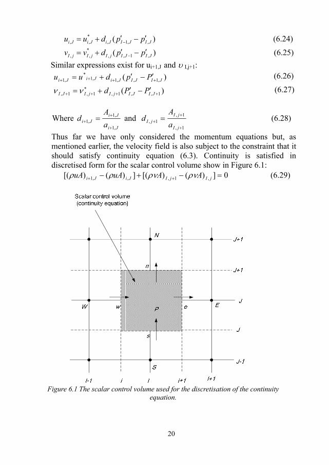
Thus far we have only considered the momentum equations but, as mentioned earlier, the velocity field is also subject to the constraint that it should satisfy continuity equation (6.3). Continuity is satisfied in discretised form for the scalar control volume show in Figure 6.1:

0])()[(])()[( ,1,,,1 =−+− ++ jIjIJiJi AAuAuA ρνρνρρ (6.29)

Figure 6.1 The scalar control volume used for the discretisation of the continuity

equation.

21

Substitution of the corrected velocities of equations (6.24-6.27) into discretised continuity equation (6.29) gives

1, 1, 1, 1 , 1,

J , , , I 1 J ,

, 1 I , 1 , 1 , , 1

, , , , , 1 ,

[ A ( ( ))

A ( ( ))]

[ A ( ( ))

( ( ))] 0

i J i J i J i I J I J

i i J i J i J I J

I j I j I j I J I J

I j i j i j I j I J I J

u d p p

u d p p

d p p

A d p p

ρ

ρ

ρ ν

ρ ν

∗+ + + + +

∗−

∗+ + + +

∗ ∗−

′ ′+ −

′ ′− + −

′ ′+ + −

′ ′− + − =

，J

， ，

，j +1

(6.30)

This may be re-arranged to give

, 1

1, , , 1 ,

1, 1, , 1, , 1

, 1, , , 1

[( ) ( ) ( ) ( ) ]

(( ) ( ) ( )

[( ) ( ) ( ) ( ) ]I j

i J i J I j I j

i J I J i J i J I J

i J i J I j I j

dA dA dA dA

dA p dA p dA p

u A u A A A

ρ ρ ρ ρ

ρ ρ ρ

ρ ρ ρν ρν+

+ +

+ + − +

∗ ∗ ∗ ∗+ +

+ + +

′ ′ ′= + +

+ − + −

(6.31)

Identifying the coefficients of p′ this may be written as

, , 1, 1, 1, 1, , 1 , 1

, 1 , 1 ,

I J I J I J I J I J I J I J I J

I J I J I J

a p a p a p a pa p b

+ + − − + +

− −

′ ′ ′ ′= + +

′ ′+ + (6.32)

Where , 1, 1, , 1 , 1I J I J I J I J I Ja a a a a+ − + −= + + + and the coefficients are given below:

1,I Ja + 1,I Ja − , 1I Ja + , 1i Ja −

1,( )i JdAρ + ,( )i JdAρ , 1( )I jdAρ + ( )dAρ I , j

,I Jb′

, 1, , , 1( ) ( ) ( ) ( )i J i J I j I ju A u A A Aρ ρ ρν ρν∗ ∗ ∗ ∗+ +− + −

Equation (6.32) represents the discretised continuity equation as an equation for pressure correction p′ . The source term b′ in the equation is the continuity imbalance arising from the incorrect velocity field u∗ ,ν ∗ , By solving equation (6.32), the pressure correction field p′ can be obtained at all points. Once the pressure correction field is known, the correct pressure field may be obtained using formula (6.14) and velocity components through correction formulae (6.24-6.27). The omission of terms such as

nb nba u′∑ in the derivation does not affect the final solution because the pressure correction and velocity corrections will all be zero in a converged solution giving p p∗ = ,u u∗ = andν ν∗ = . The pressure correction equation is susceptible to divergence unless some under-relaxation is used during the iterative process and new, improved,

22

pressures newp are obtained with new

pp p a p∗ ′= + (6.33) Where pα is the pressure under-relaxation factor. If we select pα equal to I

the guessed pressure field p∗ is corrected by p′ . However, the corrections p′ , in particular when the guessed field p∗ is far away from the final solution, is often too large for stable computations. A value of pα equal to zero would apply no correction at all, which is also undesirable. Taking pα between 0 and 1 allows us to add to guessed field p∗ a fraction of the correction field of the correction field p′ that is large enough to move the iterative improvement process forward, but small enough to ensure stable computation. The velocities are also under-relaxed. The iteratively improved velocity components newu and newν are obtained from ( 1)(1 )new n

u uu u uα α −= + − (6.34) ( 1)(1 )new n

ν νν α ν α ν −= + − (6.35) Where uα and να are the u- and ν -velocity under-relaxation factors with values between 0 and 1, u and ν are the corrected velocity components without relaxation and ( 1)nu − and ( 1)nν − represent their values obtained in the previous iteration. After some algebra it can be shown that with under-relaxation the discretised u-momentum equation takes the form

, , ( 1), 1, , , ,( ) (1 )i J i J n

i J nb nb I J I J i J i u i Ju u

a au a u p p A b u

aα

α−

−

⎡ ⎤= + − + + −⎢ ⎥

⎣ ⎦∑ ，J (6.36)

and the discretised ν -momentum equation

, , ( 1), , 1 , , , ,( ) (1 )I j I j n

I j nb nb I J I J I j I j I j

a aa p p A b

a νν ν

ν ν α να

−−

⎡ ⎤= + − + + −⎢ ⎥

⎣ ⎦∑ (6.37)

The pressure correction equation is also affected by velocity under-relaxation and it can be shown that d-terms of pressure correction equation become

,,

,

i J ui J

i J

Ad

aα

= , 1,1,

1,J

i J ui J

i

Ad

aα+

++

= , ,,

,

I jI j

I j

Ad

aνα=

and

23

, 1, 1

, 1

I jI j

I j

Ad

aνα+

++

=

Note that in these formulae ,i Ja , 1,i Ja + , ,I ja and , 1I ja + are the central coefficients of discretised velocity equations at positions (i,J), (i+1,J), (I,j) and (I,j+1) of a scalar cell centered around P. A correct choice of under-relaxation factors α is essential for cost-effective simulations. Too large a value of α may lead to oscillatory or even divergent iterative solutions and a value which is too small will cause extremely slow convergence. Unfortunately, the optimum values of under-relaxation factors are flow dependent and must be sought on a case-by-case basis. The SIMPLE algorithm gives a method of calculating pressure and velocities, The method is iterative and when other scalars are coupled to the momentum equations, the calculation needs to be done sequentially. The sequence of operations in a CFD procedure which employs the SIMPLE algorithm is given in Figure 6.2

24

Initial guess , , ,p u ν∗ ∗ ∗ ∗∅ ,u ν∗ ∗ ,u ν∗ ∗ p′ , , ,p u ν ∗∅ No ∅ yes

Figure 6.2 the SIMPLE Algorithm Flow chart

START

SETP 3: Correct pressure and velocities , , ,

, , , 1, ,

, , , 1, ,

( )

( )

I J I J I J

I J i J i J I J I J

I j I j i J I J I J

p p p

u u d p p

d p pν ν

∗

∗−

∗−

′= +

′ ′= + −

′ ′= + −

STEP 1：Solve discretised momentum equations

, , 1, , , ,( )i J i J nb nb I J I J i J i Ja u a u p p A b∗ ∗ ∗ ∗−= + − +∑

, , , 1 , , ,( )I J I J nb nb I J I J I J I Ja a p p A bν ν∗ ∗ ∗ ∗−= + − +∑

STEP 2: Solve pressure correction equation , , 1, 1, 1, 1, , 1 , 1 , 1 , 1 ,I J I J I J I J I J I J I J I J I J I J I Ja p a p a p a p a p b− − + + − − + +′ ′ ′ ′ ′ ′= + + + +

STEP 4：Solve all other discretised transport equations , , 1, 1, 1, 1, , 1 , 1 , 1 , 1 ,I J I J I J I J I J I J I J I J I J I J I Ja a a a a b− − + + − − + +∅ = ∅ + ∅ + ∅ + ∅ + ∅

Convergence?

STOP

,,

SetP p u uν ν

∗ ∗

∗ ∗

= =

= ∅ =∅

25

6.3 Implementation of boundary conditions

6.3.1 Grid arrangement

• The physical boundary coincide with the scalar control volume • The grid extends outside the physical boundary.

6.3.2 Inlet boundary conditions

To accommodate the inlet boundary condition for these variables, it is unnecessary to make any modifications to their discretized equations. The link with the boundary side is cut in the discretized pressure correction equation by setting the boundary side coefficient aw (if the inlet is on the west) equal to zero. Since the velocity is known at inlet, it is also not necessary to make a velocity correction here and hence we have *

w wu u=

6.3.3 Outlet boundary conditions

The outlet is such a region that the flow often teaches a fully developed state where no change occurs in the flow direction. It means all the variables (except pressure), the gradient is 0. For the v- and scalar equations this implies setting , 1, , 1, ; NI j NI j NI J NI Jv v φ φ− −= =

Where NI is the last line of the nodes. Special care should be taken in the case of the u-velocity. Calculation of u at the outlet plane i=NI by assuming a zero gradient gives , 1,NI j NI ju u −=

During the iteration cycles of the SIMPLE algorithm there is no guarantee that these velocities will conserve mass over the computational domain as a whole. To ensure that overall continuity is satisfied the total mass flux going out of the domain (Mout ) is firstly computed by summing all the extrapolated outlet velocities. To make the mass flux out equal to the mass flux Min coming into the domain all the outlet velocity components uNI, J are multiplied by the ratio Min/ Mout. Thus the outlet plane velocities with the continuity correction are given by

26

, 1, / NI j NI j in outu u M M−= ×

The velocity at the outlet boundaries is not corrected by means of pressure corrections. Hence in the discretised p’-equation the link to the outlet (if it is on the east) boundary side is suppressed by setting aE=0. The contribution to the source term in this equation is calculated as normal, noting that *

E Eu u= No addition modifications are required.

6.4.4 Outlet boundary conditions

The wall is the most common boundary encountered in confined fluid flow problems. The no-slip condition is the appropriate condition for the velocity components at solid walls. Which is

u=v=0

Since the wall velocity is known, it is also unnecessary to perform a pressure correction here. In the discretised p’-equation for the cell nearest to the wall, the wall link (if it is on the south) is cut by setting aS = 0, and in the source term

*S Sv v=

6.4 Drying in Straight Pipe Model

The straight type is the common type which is too high, often difficult to fabricate in the workshop is shown in the diagram below

27

Figure 6.3 straight type dryer Kunming shipbuilding equipment Co In the above equipment，only the cavity where drying occur; that is, the part labeled straight pipe dryer is modeled and solved in Fluent and hand written code is used to validate the solution. The results of the single and double phase are presented in chapter 8. However, other components shown in the above picture are mechanisms for

28

the transportation of the particles and gas; to and away from, the drying chamber, and also the separator.

6.4.1 Straight pipe model in Gambit

Figure 6.4 section of straight type dryer

Above figure the model of the straight pipe imported to FLENT from GAMBIT with positive Z axis pointing downward.

6.5 Design and Working Principle of the Screw Dryer

The screw dryer is basically a cylindrical, conical shell; Products are to be fed into the cyclone dryer pneumatically together with the drying air via a

29

rectangular inlet. Entering sideways tangentially into the dryer, the conveying air gets a strong rotational spin. The rotational movement continues to the end or outlet of the dryer, Due to the rotational movement, products are successively separated from the drying air by centrifugal force, and then re-mixed into the gas flow, following the declination to the outlet. The high relative velocities and temperature between particles and drying air, is responsible for the successive separation, and reintroduction of the solid and ensure high heat and mass transfer coefficients. At the dryer outlet, the dry products are collected as result of separation from the hot gas, but the mechanism is not included in this work.. Different models were tried like the perfect cylindrical shape type, with tangential inlet, and also, a model without inner cylinder (see appendices for pictures), but the conical bottom and inner confirmed cylinder gives screw dryer a better or more uniform outlet time The screw dryer is a compact and simple device. It contains no moving parts it is of a lower height, requires no extra control and can be fabricated in the workshop. See diagram below

Figure 6.5 model of The screw dryer

30

7 Simulation

7.1 Choice of commercial software

The validation work was carried out in FLUENT which is computational fluid dynamics softwear, which helps to analyze systems involving fluid flow, heat transfer and associated phenomena, such as chemical reactions by means of computer base simulation, based on finite volume method. The model was created in GAMBIT another software which is a pre-processing tool to FLUENT. The result from simulations are compared with solution from the matlab code.

7.2 Problem Formulation /Definition (in commercial software)

The model dryer, was created, and the effect of boundary layer applied and meshed with tetrahedral element, in GAMBIT software, and exported as a mesh file.

The created mesh file was read into FLUENT as a case file and the dimensions are checked if it conform with that created in GAMBIT.

Segregated, implicit and steady solver chosen as the solver in FLUENT.

The flow was modeled as turbulent, and K-epsilon was used.

From the material in FLUENT hydrogen air was chosen.

Energy and the boundary condition panel was activated.

7.3 Boundary Conditions

The (absolute) pressure at the outlet is 1 atm. Since the operating pressure

31

is set to 1 atm, the outlet gauge pressure = outlet absolute pressure - operating pressure = 0. No back flow. And the inlet velocity and temperature are 18m/s and 600 degree Kelvin respectively; while the wall is of constant temperature of 300 degree Kelvin, that is; adiabatic, stationary and no slip wall, impermeable to flow modeled in the Z direction.

7.4 Assumptions

Particles are assumed spherical, and of uniform diameters. Steady flow of gas particles was assumed. Friction occurs between the wall and gas, solid particles, i.e boundary layer phenomena.

7.5 Postprocessing

The solution was initialized from the inlet, under the solution control discrete phase source was taken as 0.1 and the convergence check criteria was set at 0.001 which is good enough to ensure accurate result.

32

8 Result and Analysis

8.1 Single phase

The figures below shows the results of plots obtained, for single phase from matlab code with data from the factory where the symmetry of the problem is applied and the residence time of the gas particle，And also single phase analysis obtained from FLUENT, and the result show almost perfect agreement.

Figure 8.1 plot from matlab Figure 8.1 shows Result of single phase calculated from matlab, symmetry of the problem was applied. It shows the temperature background with velocity foreground. Static pressure, residual plot and mass flow accumulation which remain constant after about 100 step and it is used for the residence time calculation

33

Figure 8.2 temperature plot in FLUENT See appendices A for the pressure plot. The pressure plot of the matlab and FLUENT shows slight variation from the matlab script but the temperature and residence time are the same.

34

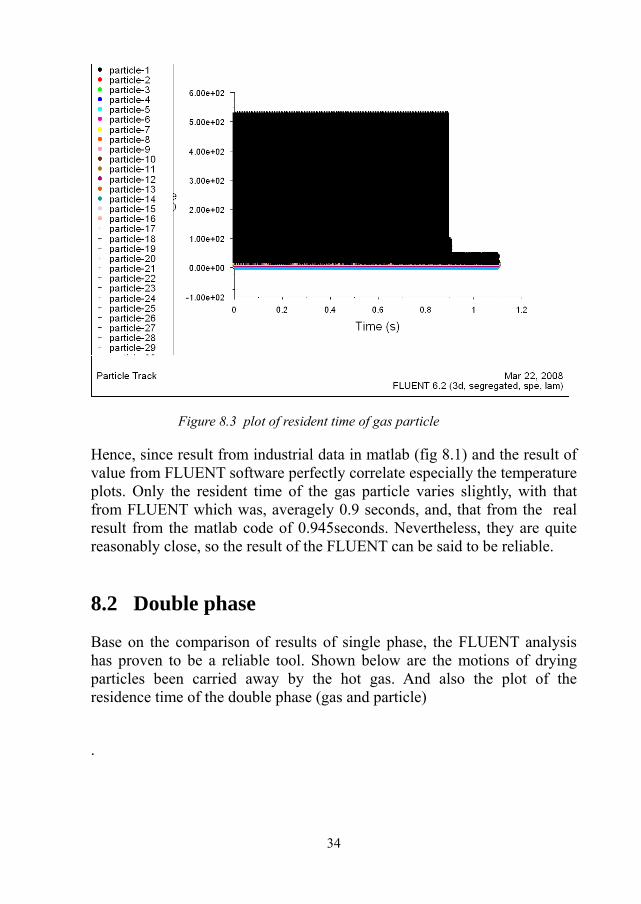
Figure 8.3 plot of resident time of gas particle Hence, since result from industrial data in matlab (fig 8.1) and the result of value from FLUENT software perfectly correlate especially the temperature plots. Only the resident time of the gas particle varies slightly, with that from FLUENT which was, averagely 0.9 seconds, and, that from the real result from the matlab code of 0.945seconds. Nevertheless, they are quite reasonably close, so the result of the FLUENT can be said to be reliable.

8.2 Double phase

Base on the comparison of results of single phase, the FLUENT analysis has proven to be a reliable tool. Shown below are the motions of drying particles been carried away by the hot gas. And also the plot of the residence time of the double phase (gas and particle) .

35

Figure 8.4 The resident time of drying particle From the above plot, figure 8.4; it shows simulated drying time of particle as 5.2 seconds which is slightly different from the real industrial value of 7 seconds.

36

8.3 Swirling type double phase

Figure 8.5 Swirling type double phase Above figure shows the part of motion, of particle inside the swirling dryer type with a reduce height and with approximately the same particle traveling distance as the straight type, swirling is as a result of tangential inlet motion of the hot gas and particle.

37

Figure 8.6 the time of swirling type model Above is the residence time of swirling dryer type. However, due to the tangential inlet, the outlet of particles are not uniform as the straight type; nevertheless, the average time is about 7seconds which is good for the analyses ,in comparison to real value.

38

9 Conclusions and future work

9.1 conclusion

This study basically used the drying time, pressure, temperature to analyze the effectiveness of drying equipment; other drying factors such as porosity, initial moisture, final moisture content, diffussibilty of the material are not considered. It revealed that the new swirling model work effectively as the straight type. And the result obtained from FLUENT is reliable base on the comparison with the matlab code so, further analysis is recommended in FLUENT. Also, it should be noted that spherical wood of appreciable uniform diameter was used from FLUENT material data base to simulate the drying particle. However, the slight difference in the industrial drying time and the simulated drying time, could be due to difference in material properties such as; weight difference as a result of irregular or non- uniform size of real particles. Nevertheless, the final drying time is close enough to be accepted.

9.2 Further work

1. Re-design the swirling type dryer to give a uniform precise drying time like the straight type

2. The porosity, diffusivity can be considered to give this swirling type a generalized application.

3. The mechanism of separating the dried product from the hot gas can be included in the future work.

39

10 REFERENCES 1. Chou, S.K.; Chua, K.J, New hybrid drying technologies for heat sensitive foodstuffs, Trends in Food Science & Technology 2001, 2. Kudra,T,Mujumdar,A.S.‘AdvancedDrying Technologies Marcel Dekker, Inc.: New York, 2002; 81–111. 3. S.H Hyun, T.Y Kim, G.S Kim and H. Park, Synthesis of low-k Porous Silica films via freeze Drying. J. material science 19. 4 Thermal Control of Freeze-Drying processes in a porous Medium With predetermined. S. Lin, Rate of Drying . Int .J Refrg 18. 5. X.L. Huai, X.F. Peng, G.X Wang and D.Y Liu Multiphase Flow and drying Characteristics In A Semi-circular Impinging Stream Dryer . 6. Kemp, Ian C. (2007) 'Drying Software: Past, Present, and Future', Drying Technology, 25:7, 1249 – 1263 7. Portter, M.C and Wiggert, D.C 2003 Mechanism of fluids, China Machine Press. 8. R. Najmur, and K. Subodh Influence of Sample Size and Shape on transport Parameters Durring Drying of Shrinking Bodies 9. Saravanan, B. Balasuramaian, N and Srinivasakannan, C, Drying Kinectics In A Vertical Gas-Solid System, Chem. Eng. Technology 2007, 30, No.2, 176-183 10. P. Somkiat, T. Warunee, P. Korakot, and S. Somchart Comparison of performances of pulsed and conventional fluidised-bed dryer. 11. M.C Ferreira, E.V. Silva, and J.T Freire Analysis of One Dimensional Fluid Dynamic Model In A Pneumatic Dryer With A Spouted Bed Type Solid Feeding System, Drying technology, 16:9 1971-1985 12. J. Ali , T. Hitham, A. Ahmad and A. Ababneh, Strongly swirling flow 13. Broman. G. 2003 Computational Engineering. Department of Mechanical Engineering Blekinge Institute of Technology. Karlskrona, Sweden . 14 S. A. Giner, D.M. Bruce, S. Mortimore Two-dimemsional Simulation of Steady-state Mixed-flow Grain Drying Part 1 The model 15. Avil L. Thomas M. Predrag M. and David J.M, ‘ A Comparison Of analytical Model With Experimental Data For Gas-solid Flow Through A Straight pipe At Different Inclinations ‘ powder Technology. 16. C. Strumillo, T. Kudra, Drying: Principles ,Applications and Design, Gordeon and Newyork 1986. 17. Versteeg H. K .and Malalasekera. Introduction To Computational Fluid

40

Dynamics The Finite Volume Methods’ Prentice Hall .

41

11. APPENDICES

A. OTHER TRIES in FLUENT

Below are other model but with defect result

42

Motion of particle in the new design

Motion of particle carried by hot gas in a straight pipe with outlet red and inlet blue and particles multi-color shown in the

43

Pressure contours in FLUENT

44

45

B. MATLAB CODE

%%%%%SIMPLE.m clc,clear all,close all global l1 m1 xl yl rhocon xl=1; yl=16;m1=28;l1=28;rhocon=1; default_setting; user_could_reset_some_setting_here generate_grid user_initial_grid_value figure set(gca,’nextplot’,’replacechildren’); for iter=1:last [rho]=user_correct_density(rhot,t); iter1=1; smax=1; while smax>0.001 [v,t,factor,flowin]=user_bound_condition_setup(l1,l2,rho,v,t,xcv,m1,m2,iter1,flowin); setupcoef; [v,t,factor,flowin]=user_bound_condition_setup(l1,l2,rho,v,t,xcv,m1,m2,iter1,flowin); disp([’Time step:’ int2str(iter) ’ substep=’ int2str(iter1) ’ smax=’ num2str(smax)]); iter1=iter1+1; end [rho]=user_correct_density(rhot,t);

46

user_output; masscount Fr(iter) = getframe; time=time+dt; end %%%%% default_setting.m global m1 l1 l2=l1−1; l3=l2−1; m2=m1−1; m3=m2−1; nfmax=10; np=11; nrho=12; ngam=13; smax=1; ssum=1; flowin=0; lstop=0;

for i=1:1 relax(i)=1; end mode=1; time=0; ipref=1; jpref=1; rhocon=1; %%%%%%user_could_reset_some_setting_here relax(1)=0.5;

relax(2)=0.5; relax(11)=0.8; mode=1;

47

last=300; pr=0.85; amu=1.72e−5; amup=amu/pr; tref=300; rhoref=1.29;

rhot=rhoref*tref; dt=0.005; for i=1:nfmax ntimes(i)=30; end %%%%%generate_grid global m1 l1 rhocon [xu,yv]=user_generate_velocity_grid; l2=l1−1; l3=l2−1; m2=m1−1; m3=m2−1; x(1)=xu(1); for i=2:l2 x(i)=0.5*(xu(i+1)+xu(i)); end x(l1)=xu(l1); y(1)=yv(2); for j=2:m2 y(j)=0.5*(yv(j+1)+yv(j)); end y(m1)=yv(m1); z=3*ones(m1,l1); [X,Y]=meshgrid(x,y);surf(X,Y,z); view(0,90);%axis equal caxis([0 3.9]) hold on S=zeros(m1,l1);

48

for j=2:m2 for i=2:l2 S(i,j)=1;Sc(i−1,j−1)=1; plot3(x(i),y(j),z(j,i),’o’); end end U=zeros(m1,l1); for j=2:m2 for i=3:l2 U(i,j)=1;Uc(i−2,j−1)=1; plot3(xu(i),y(j),z(j,i),’s’) end end V=zeros(m1,l1); for j=3:m2 for i=2:l2 V(i,j)=1;Vc(i−1,j−2)=1; plot3(x(i),yv(j),z(j,i),’x’,’markersize’,9) end end for i=2:l1 xdif(i)=x(i)−x(i−1); end for i=2:l2 xcv(i)=xu(i+1)−xu(i); end xcvs(3)=xdif(2)+xdif(3); for i=4:(l2−1) xcvs(i)=xdif(i); end xcvs(l2)=xdif(l2)+xdif(l1); xcvip=zeros(1,l1); for i=3:l3 xcvi(i)=0.5*xcv(i); xcvip(i)=xcvi(i);

49

end xcvip(2)=xcv(2); xcvi(l2)=xcv(l2); for j=2:m1 ydif(j)=y(j)−y(j−1); end for j=2:m2 ycv(j)=yv(j+1)−yv(j); end ycvs(3)=ydif(2)+ydif(3); for j=4:m3 ycvs(j)=ydif(j); end ycvs(m2)=ydif(m2)+ydif(m1); for j=2:m2 ycvr(j)=ycv(j); arx(j)=ycvr(j); end ycvrs(3)=ycvs(3); for j=3:m3 ycvrs(j)=ydif(j); end ycvrs(m2)=ycvs(m2); arxjp(2)=arx(2); for j=3:m3 arxj(j)=0.5*arx(j); arxjp(j)=arxj(j); end arxj(m2)=arx(m2); for j=3:m3 fv(j)=arxjp(j)/arx(j); fvp(j)=1.0−fv(j);

50

end for i=3:l2 fx(i)=0.5*xcv(i−1)/xdif(i); fxm(i)=1.0−fx(i); end fx(2)=0.0; fxm(2)=1; fx(l1)=1.0; fxm(l1)=0.0; for j=3:m2 fy(j)=0.5*ycv(j−1)/ydif(j); fym(j)=1.0−fy(j); end fy(2)=0.0; fym(2)=1.0; fy(m1)=1.0; fym(m1)=0.0; for j=1:m1 for i=1:l1 pc(i,j)=0; u(i,j)=0; v(i,j)=0; p(i,j)=0; con(i,j)=0; ap(i,j)=0; rho(i,j)=rhocon; end end %%%%%user_initial_grid_value tin=600.0;tw=300.0;vin=18.0;

51

inletwidth=0; for i=2:l2 inletwidth=inletwidth+xcv(i); end vout=vin*inletwidth/x(l1)*tw/tin; for j=1:l1 for i=1:m1 u(i,j)=0; v(i,j)=vout; v(1,j)=0; v(i,2)=0; t(i,j)=tw; end end for i=2:l2 v(i,2)=vin; t(i,1)=tin; end %%%%% function [xu,yv]=user_generate_velocity_grid global xl yl m1 l1 xu(2)=0; dx=xl/(l1−2); for i=3:l1 xu(i)=xu(i−1)+dx; end yv(2)=0; dy=yl/(m1−2); for j=3:m1 yv(j)=yv(j−1)+dy;

52

end %%%%% function [rho]=user_correct_density(rhot,t) global m1 l1 for j=1:m1 for i=1:l1 rho(i,j)=rhot/t(i,j); end end %%%%% function [acof]=diflow(diff, flow) acof=diff; if flow==0 return; end temp=diff−abs(flow)*0.1; acof=0.0; if temp<0 return; end temp=temp/diff; acof=diff*temp^5; %%%%% function [gam]=user_gamsor(amu,amup,nf) global m1 l1 for j=1:m1 for i=1:l1 gam(i,j)=amu; if nf==4 gam(i,j)=amup; end if nf~=1 gam(l1,j)=0; end

53

gam(i,m1)=0; end end

end

%%%%% function [v,t,factor,flowin]=user_bound_condition_setup(l1,l2,rho,v,t,xcv,m1,m2,iter1,flowin); inletgridindex=fix(l1/8); if iter1==1 flowin=0; for i=2:l2 flowin=flowin+rho(i,1)*v(i,2)*xcv(i); end end fl=0; for i=2:l2 fl=fl+rho(i,m1)*v(i,m2)*xcv(i); factor=flowin/fl; end for i=2:l2 v(i,m1)=v(i,m2)*factor; t(i,m1)=t(i,m2); end for j=3:m2 v(l1,j)=v(l2,j); end for j=2:m2 t(l1,j)=t(l2,j); end %%%%%setupcoef.m ap=zeros(m1,l1);aim=zeros(m1,l1);aip=zeros(m1,l1);

54

ajp=zeros(m1,l1);ajm=zeros(m1,l1);con=zeros(m1,l1); nf=1; apt=zeros(m1,l1); ist=3; jst=2; [gam]=user_gamsor(amu,amup,nf); %gam rel=1.0−relax(nf); for i=3:l2 fl=xcvi(i)*v(i,2)*rho(i,1); flm=xcvip(i−1)*v(i−1,2)*rho(i−1,1); %FLOW=R(1)*(FL+FLM); flow=(fl+flm); %DIFF=R(1)*(XCVI(I)*GAM(I,1)+XCVIP(I−1)*GAM(I−1,1))/YDIF(2) diff=(xcvi(i)*gam(i,1)+xcvip(i−1)*gam(i−1,1))/ydif(2); [acof]=diflow(diff, flow); ajm(i,2)=acof+max(0,flow); end for j=2:m2 flow=arx(j)*u(2,j)*rho(1,j); %DIFF=ARX(J)*GAM(1,J)/(XCV(2)*SX(J)) diff=arx(j)*gam(1,j)/(xcv(2)); [acof]=diflow(diff, flow); aim(3,j)=acof+max(0,flow); for i=3:l2 if(i==l2) flow=arx(j)*u(l1−1,j)*rho(l1−1,j); %DIFF=ARX(J)*GAM(L1,J)/(XCV(L2)*SX(J)) diff=arx(j)*gam(l1,j)/(xcv(l2)); else

55

fl=u(i,j)*(fx(i)*rho(i,j)+fxm(i)*rho(i−1,j)); flp=u(i+1,j)*(fx(i+1)*rho(i+1,j)+fxm(i+1)*rho(i,j)); flow=arx(j)*0.5*(fl+flp); %DIFF=ARX(J)*GAM(I,J)/(XCV(I)*SX(J)) diff=arx(i)*gam(i,j)/(xcv(j)); end [acof]=diflow(diff, flow); aim(i+1,j)=acof+max(0.0,flow); aip(i,j)=aim(i+1,j)−flow; if (j==m2) fl=xcvi(i)*v(i,m1)*rho(i,m1); flm=xcvip(i−1)*v(i−1,m1)*rho(i−1,m1); %DIFF=R(M1)*(XCVI(i)*GAM(I,M1)+xcvip(i−1)*GAM(I−1,M1))/YDIF(M1) diff=(xcvi(i)*gam(i,m1)+xcvip(i−1)*gam(i−1,m1))/ydif(m1); else fl=xcvi(i)*v(i,j+1)*(fy(j+1)*rho(i,j+1)+fym(j+1)*rho(i,j));%=============== flm=xcvip(i−1)*v(i−1,j+1)*(fy(j+1)*rho(i−1,j+1)+fym(j+1)*rho(i−1,j)); gm=gam(i,j)*gam(i,j+1)/(ycv(j)*gam(i,j+1)+ycv(j+1)*gam(i,j)+1.0e−30)*xcvi(i);% gmm=gam(i−1,j)*gam(i−1,j+1)/(ycv(j)*gam(i−1,j+1)+ycv(j+1)*gam(i−1,j)+1.e−30)*xcvip(i−1); %diff=rmn(j+1)*2.*(gm+gmm); diff=2*(gm+gmm); end %flow=rmn(j+1)*(fl+flm); flow=(fl+flm); [acof]=diflow(diff, flow); ajm(i,j+1)=acof+max(0.0,flow); %as ajp(i,j)=ajm(i,j+1)−flow; %an

56

vol=ycvr(j)*xcvs(i); apt=(rho(i,j)*xcvi(i)+rho(i−1,j)*xcvip(i−1))/(xcvs(i)*dt); ap(i,j)=ap(i,j)−apt; con(i,j)=con(i,j)+apt*u(i,j); ap(i,j)=(−ap(i,j)*vol+aip(i,j)+aim(i,j)+ajp(i,j)+ajm(i,j))/relax(nf); con(i,j)=con(i,j)*vol+rel*ap(i,j)*u(i,j); %b=Sc+ap0*¦μp0*(1−relax) %DU(I,J)=VOL/(XDIF(I)*SX(J)) rel=1.0−relax(nf); du(i,j)=vol/(xdif(i)); con(i,j)=con(i,j)+du(i,j)*(p(i−1,j)−p(i,j)); du(i,j)=du(i,j)/ap(i,j); %du=dw=de end%for i end%for j f(:,:,1)=u(:,:); tsolve u(:,:)= f(:,:,1); nf=2; ist=2; jst=3; [gam]=user_gamsor(amu,amup,nf); rel=1.0−relax(nf); for i=2:l2 %AREA=R(1)*XCV(I) area=xcv(i); flow=area*v(i,2)*rho(i,1); diff=area*gam(i,1)/ycv(2); [acof]=diflow(diff, flow); ajm(i,3)=acof+max(0.0,flow); end for j=3:m2

57

fl=arxj(j)*u(2,j)*rho(1,j); flm=arxjp(j−1)*u(2,j−1)*rho(1,j−1); flow=fl+flm; %DIFF=(ARXJ(J)*GAM(1,J)+ARXJP(J−1)*GAM(1,J−1))/(XDIF(2)*SXMN(J)) diff=(arxj(j)*gam(1,j)+arxjp(j−1)*gam(1,j−1))/(xdif(2)); [acof]=diflow(diff, flow); aim(2,j)=acof+max(0.0,flow); for i=2:l2 if i==l2 fl=arxj(j)*u(l1,j)*rho(l1,j); flm=arxjp(j−1)*u(l1,j−1)*rho(l1,j−1); %DIFF=(ARXJ(J)*GAM(L1,J)+ARXJP(J−1)*GAM(L1,J−1))/(XDIF(L1)*SXMN(J)) diff=(arxj(j)*gam(l1,j)+arxjp(j−1)*gam(l1,j−1))/(xdif(l1)); else fl=arxj(j)*u(i+1,j)*(fx(i+1)*rho(i+1,j)+fxm(i+1)*rho(i,j)); flm=arxjp(j−1)*u(i+1,j−1)*(fx(i+1)*rho(i+1,j−1)+fxm(i+1)*rho(i,j−1)); gm=gam(i,j)*gam(i+1,j)/(xcv(i)*gam(i+1,j)+xcv(i+1)*gam(i,j)+1.e−30)*arxj(j); gmm=gam(i,j−1)*gam(i+1,j−1)/(xcv(i)*gam(i+1,j−1)+xcv(i+1)*gam(i,j−1)+1.0e−30)*arxjp(j−1); %DIFF=2.*(GM+GMM)/SXMN(J) diff=2*(gm+gmm); end flow=fl+flm; [acof]=diflow(diff, flow); aim(i+1,j)=acof+max(0.0,flow); aip(i,j)=aim(i+1,j)−flow; if j==m2

58

%AREA=R(M1)*XCV(I) area=xcv(i); flow=area*v(i,m1)*rho(i,m1); diff=area*gam(i,m1)/ycv(m2); else area=xcv(i); %fl=v(i,j)*(fy(j)*rho(i,j)+fym(j)*rho(i,j−1))*rmn(j); %flp=v(i,j+1)*(fy(j+1)*rho(i,j+1)+fym(j+1)*rho(i,j))*rmn(j+1); fl=v(i,j)*(fy(j)*rho(i,j)+fym(j)*rho(i,j−1)); flp=v(i,j+1)*(fy(j+1)*rho(i,j+1)+fym(j+1)*rho(i,j)); flow=(fv(j)*fl+fvp(j)*flp)*xcv(i); diff=area*gam(i,j)/ycv(j); end [acof]=diflow(diff, flow); ajm(i,j+1)=acof+max(0.0,flow); ajp(i,j)=ajm(i,j+1)−flow; vol=ycvrs(j)*xcv(i); apt=(arxj(j)*rho(i,j)+arxjp(j−1)*rho(i,j−1))/(ycvrs(j)*dt); ap(i,j)=ap(i,j)−apt; con(i,j)=con(i,j)+apt*v(i,j); ap(i,j)=(−ap(i,j)*vol+aip(i,j)+aim(i,j)+ajp(i,j)+ajm(i,j))/relax(nf); con(i,j)=con(i,j)*vol+rel*ap(i,j)*v(i,j); dv(i,j)=vol/ydif(j); con(i,j)=con(i,j)+dv(i,j)*(p(i,j−1)−p(i,j)); dv(i,j)=dv(i,j)/ap(i,j); % dv=ds=dn end %for i end%for j f(:,:,2)=v(:,:); tsolve v(:,:)= f(:,:,2); nf=3;

59

ist=2; jst=2; [gam]=user_gamsor(amu,amup,nf); smax=0; ssum=0; for j=2:m2 for i=2:l2 vol=ycvr(j)*xcv(i); con(i,j)=con(i,j)*vol; end end for i=2:l2 arho=xcv(i)*rho(i,1); con(i,2)=con(i,2)+arho*v(i,2); ajm(i,2)=0; end for j=2:m2 arho=arx(j)*rho(1,j); con(2,j)=con(2,j)+arho*u(2,j); aim(2,j)=0; end%=== for j=2:m2 %=== for i=2:l2 if(i==l2) arho=arx(j)*rho(l1,j); con(i,j)=con(i,j)−arho*u(l1,j); aip(i,j)=0; else arho=arx(j)*(fx(i+1)*rho(i+1,j)+fxm(i+1)*rho(i,j)); flow=arho*u(i+1,j); con(i,j)=con(i,j)−flow; con(i+1,j)=con(i+1,j)+flow; aip(i,j)=arho*du(i+1,j);

60

aim(i+1,j)=aip(i,j); end end%=== end%=== for j=2:m2 %=== for i=2:l2 %=== if j==m2 %ARHO=RMN(M1)*XCV(I)*RHO(I,M1) arho=xcv(i)*rho(i,m1); con(i,j)=con(i,j)−arho*v(i,m1);%Ô´ÏîbÀÛ¼Ó ajp(i,j)=0; else %ARHO=RMN(J+1)*XCV(I)*(FY(J+1)*RHO(I,J+1)+FYM(J+1)*RHO(I,J)) arho=xcv(i)*(fy(j+1)*rho(i,j+1)+fym(j+1)*rho(i,j)); flow=arho*v(i,j+1); con(i,j)=con(i,j)−flow; con(i,j+1)=con(i,j+1)+flow; ajp(i,j)=arho*dv(i,j+1); ajm(i,j+1)=ajp(i,j); end

ap(i,j)=aip(i,j)+aim(i,j)+ajp(i,j)+ajm(i,j); pc(i,j)=0; smax=max(smax,abs(con(i,j))); ssum=ssum+con(i,j); end %for i end%for j f(:,:,3)=pc(:,:); tsolve pc(:,:)= f(:,:,3); for j=2:m2 for i=2:l2 p(i,j)=p(i,j)+pc(i,j)*relax(np); if i~=2 u(i,j)=u(i,j)+du(i,j)*(pc(i−1,j)−pc(i,j)); end if j~=2

61

v(i,j)=v(i,j)+dv(i,j)*(pc(i,j−1)−pc(i,j)); end end end ist=2; jst=2; nf=4; [gam]=user_gamsor(amu,amup,nf); rel=1−relax(nf); for i=2:l2 %AREA=R(1)*XCV(I) area=xcv(i); flow=area*v(i,2)*rho(i,1); diff=area*gam(i,1)/ydif(2); [acof]=diflow(diff, flow); ajm(i,2)=acof+max(0,flow); %as end for j=2:m2 flow=arx(j)*u(2,j)*rho(1,j); %DIFF=ARX(J)*GAM(1,J)/(XDIF(2)*SX(J)) diff=arx(j)*gam(1,j)/(xdif(2)); [acof]=diflow(diff, flow); aim(2,j)=acof+max(0,flow); %aw for i=2:l2 if(i==l2) flow=arx(j)*u(l1,j)*rho(l1,j); %DIFF=ARX(J)*GAM(L1,J)/(XDIF(L1)*SX(J)) diff=arx(j)*gam(l1,j)/(xdif(l1)); else flow=arx(j)*u(i+1,j)*(fx(i+1)*rho(i+1,j)+fxm(i+1)*rho(i,j)); diff=arx(j)*2.*gam(i,j)*gam(i+1,j)/(xcv(i)*gam(i+1,j)+xcv(i

62

+1)*gam(i,j)+1.0e−30; end [acof]=diflow(diff, flow); aim(i+1,j)=acof+max(0.,flow); aip(i,j)=aim(i+1,j)−flow; %area=rmn(j+1)*xcv(i); area=xcv(i); if(j==m2) flow=area*v(i,m1)*rho(i,m1); diff=area*gam(i,m1)/ydif(m1); else flow=area*v(i,j+1)*(fy(j+1)*rho(i,j+1)+fym(j+1)*rho(i,j)); diff=area*2.*gam(i,j)*gam(i,j+1)/(ycv(j)*gam(i,j+1)+ycv(j+1)*gam(i,j)+1.0e−30); end [acof]=diflow(diff, flow); ajm(i,j+1)=acof+max(0.,flow); ajp(i,j)=ajm(i,j+1)−flow; vol=ycvr(j)*xcv(i); apt=rho(i,j)/dt; ap(i,j)=ap(i,j)−apt; con(i,j)=con(i,j)+apt*t(i,j); ap(i,j)=(−ap(i,j)*vol+aip(i,j)+aim(i,j)+ajp(i,j)+ajm(i,j))/relax(nf); con(i,j)=con(i,j)*vol+rel*ap(i,j)*t(i,j); end %for i end %for j f(:,:,4)=t(:,:); tsolve t(:,:)= f(:,:,4); %%%%%tssolve.m istf=ist−1;

63

jstf=jst−1; it1=l2+ist; it2=l3+ist; jt1=m2+jst; jt2=m3+jst; for nt=1:ntimes(nf) for n=nf:nf pt(istf)=0; qt(istf)=0; for i=ist:l2 bl=0.; blp=0.; blm=0.; blc=0.; for j=jst:m2 bl=bl+ap(i,j); if j~=m2 bl=bl−ajp(i,j); end if j~=jst bl=bl−ajm(i,j); end blp=blp+aip(i,j); blm=blm+aim(i,j); blc=blc+con(i,j)+aip(i,j)*f(i+1,j,n)+aim(i,j)*f(i−1,j,n)+ajp(i,j)*f(i,j+1,n)+ajm(i,j)*f(i,j−1,n)−ap(i,j)*f(i,j,n); end denom=bl−pt(i−1)*blm; deno=1.e15; if abs(denom/bl)<1.e−10 denom=1.e20*deno; end pt(i)=blp/denom; qt(i)=(blc+blm*qt(i−1))/denom;

64

end %for i bl=0.; for ii=ist:l2 i=it1−ii; bl=bl*pt(i)+qt(i); for j=jst:m2 f(i,j,n)=f(i,j,n)+bl; end end pt(jstf)=0.; qt(jstf)=0.; for j=jst:m2 bl=0.; blp=0.; blm=0.; blc=0.; for i=ist:l2 bl=bl+ap(i,j); if i~=l2 bl=bl−aip(i,j); end if i~=ist bl=bl−aim(i,j); end blp=blp+ajp(i,j); blm=blm+ajm(i,j); blc=blc+con(i,j)+aip(i,j)*f(i+1,j,n)+aim(i,j)*f(i−1,j,n) +ajp(i,j)*f(i,j+1,n)+ajm(i,j)*f(i,j−1,n)−ap(i,j)*f(i,j,n); end denom=bl−pt(j−1)*blm; if abs(denom/bl)<1.e−10 denom=1.e20*deno; end pt(j)=blp/denom;

65

qt(j)=(blc+blm*qt(j−1))/denom; end bl=0; for jj=jst:m2 j=jt1−jj; bl=bl*pt(j)+qt(j); for i=ist:l2 f(i,j,n)=f(i,j,n)+bl; end end for j=jst:m2 pt(istf)=0.; qt(istf)=f(istf,j,n); for i=ist:l2 denom=ap(i,j)−pt(i−1)*aim(i,j); pt(i)=aip(i,j)/denom; temp=con(i,j)+ajp(i,j)*f(i,j+1,n)+ajm(i,j)*f(i,j−1,n); qt(i)=(temp+aim(i,j)*qt(i−1))/denom; end for ii=ist:l2 i=it1−ii; f(i,j,n)=f(i+1,j,n)*pt(i)+qt(i); end end %for j for jj=jst:m3 j=jt2−jj; pt(istf)=0.; qt(istf)=f(istf,j,n); for i=ist:l2

66

denom=ap(i,j)−pt(i−1)*aim(i,j); pt(i)=aip(i,j)/denom; temp=con(i,j)+ajp(i,j)*f(i,j+1,n)+ajm(i,j)*f(i,j−1,n); qt(i)=(temp+aim(i,j)*qt(i−1))/denom; end for ii=ist:l2 i=it1−ii; f(i,j,n)=f(i+1,j,n)*pt(i)+qt(i); end end %for jj for i=ist:l2 pt(jstf)=0.; qt(jstf)=f(i,jstf,n); for j=jst:m2 denom=ap(i,j)−pt(j−1)*ajm(i,j); pt(j)=ajp(i,j)/denom; temp=con(i,j)+aip(i,j)*f(i+1,j,n)+aim(i,j)*f(i−1,j,n); qt(j)=(temp+ajm(i,j)*qt(j−1))/denom; end for jj=jst:m2 j=jt1−jj; f(i,j,n)=f(i,j+1,n)*pt(j)+qt(j); end end %for i for ii=ist−1:l3 i=it2−ii; pt(jstf)=0; qt(jstf)=f(i,jstf,n); for j=jst:m2 denom=ap(i,j)−pt(j−1)*ajm(i,j); pt(j)=ajp(i,j)/denom;

67

temp=con(i,j)+aip(i,j)*f(i+1,j,n)+aim(i,j)*f(i−1,j,n); qt(j)=(temp+ajm(i,j)*qt(j−1))/denom; end for jj=jst:m2 j=jt1−jj; f(i,j,n)=f(i,j+1,n)*pt(j)+qt(j); end end end end %//for nt for j=2:m2 for i=2:l2 con(i,j)=0.; %sc=0 ap(i,j)=0.; %sp=0 aim(i,j)=0.; ajm(i,j)=0.; ajp(i,j)=0.; aip(i,j)=0.; end end

Department of Mechanical Engineering, Master’s Degree Programme Blekinge Institute of Technology, Campus Gräsvik SE-371 79 Karlskrona, SWEDEN

Telephone: Fax: E-mail:

+46 455-38 55 10 +46 455-38 55 07 ansel.berghuvud@bth.se