compton camera imaging and the cone transform a
TRANSCRIPT
COMPTON CAMERA IMAGING AND THE CONE TRANSFORM
A Dissertation
by
FATMA TERZIOGLU
Submitted to the Office of Graduate and Professional Studies ofTexas A&M University
in partial fulfillment of the requirements for the degree of
DOCTOR OF PHILOSOPHY
Chair of Committee, Peter KuchmentCommittee Members, Raytcho Lazarov
Raffaella RighettiWilliam Rundell
Head of Department, Emil Straube
May 2018
Major Subject: Mathematics
Copyright 2018 Fatma Terzioglu

ABSTRACT
In this dissertation, we focus on analytic and numerical inversion of an integral trans-
form (cone or Compton transform) that maps a function to its integrals over conical sur-
faces with a weight equal to some power of the distance from the cone’s vertex. It arises
in various imaging techniques, most prominently, in modeling of the data provided by
the so-called Compton camera, which has novel applications in various fields, including
biomedical and industrial imaging, homeland security, and gamma ray astronomy.
In the case of pure surface measure on the cone, an integral identity relating cone,
Radon and cosine transforms is presented, which enables us to derive an inversion formula
for the cone transform in any dimension. The image reconstruction algorithms, based on
the inversion formulas, and their numerical implementation results in dimensions two and
three are provided. In 3D, the implementation of the inversion algorithms is challenging
due to the high dimensionality of the forward data, and the fact that the application of a
fourth order differential operator on the unit sphere to a singular integral is required. We
thus develop and apply three different inversion algorithms and study their feasibility.
The weighted divergent beam transform, which integrates a function over rays with
a weight equal to some power of the distance to the starting point (source) of the ray, is
closely intertwined with the weighted cone transform. We study it in some details, which
leads eventually to other weighted cone transform inversions. The image reconstruction al-
gorithm, based on one of the inversion formulas, and its numerical implementation results
for various weight factors in dimensions two and three are also provided.
All inversion formulas presented in this dissertation are applicable for a wide variety
of detector geometries in any dimension.
ii

To my brilliant and loving husband Tevfik Terzioglu, and my precious son Ekin Ozan
who has been a constant source of happiness and joy since the day he came into my life
iii

ACKNOWLEDGMENTS
First and the foremost, I would like to express my deepest gratitude to my advisor Dist.
Prof. Peter Kuchment, for all his encouragement, patience and constant support during my
graduate studies. This dissertation would have never been possible without his invaluable
guidance, help and inspiration. I feel very lucky to have him as my advisor, and cannot
say enough to thank him for always being there for me.
I would like to express my sincere gratitude to Professors Raytcho Lazarov, Raffaella
Righetti and William Rundell for serving in my dissertation committee.
I am grateful to Prof. Andrea Bonito for numerous discussions and suggestions con-
cerning numerical implementation of some of the algorithms in this dissertation as well
as for his excellent instruction of partial differential equations courses. I also thank the
Numerical Analysis and Scientific Computing group for letting me use their computing
resources.
I thank Prof. Boris Rubin for many useful comments and written materials provided.
I thank Prof. Dean Baskin for his wonderful lectures on microlocal analysis.
I would like to thank the faculty and staff at the Mathematics Department of Texas
A&M University for providing an effective yet enjoyable learning environment. Special
thanks go to Prof. Peter Howard for being an excellent graduate advisor.
I would like to express my gratitude to all my teachers who put their faith in me and
urged me to do better.
I am thankful to all my friends and colleagues in College Station who have been with
me all these years and made my experience here an enjoyable and memorable one.
Special thanks go to my best friend and dear husband Tevfik Terzioglu who always
believed in me and has been a constant source of support and encouragement during the
iv

challenges of graduate school and life.
I would like to express my heartfelt gratitude to my parents, Habibe and Ibrahim Yil-
maz, and my sister Nursah Yilmaz. None of this would have been possible without their
unconditional love and continuous support.
Finally, I acknowledge the financial support provided by the Department of Mathemat-
ics and the National Science Foundation through the grant DMS 1211463.
v

CONTRIBUTORS AND FUNDING SOURCES
Contributors
This work was supervised by a dissertation committee consisting of Professors Peter
Kuchment, Raytcho Lazarov and William Rundell of the Department of Mathematics and
Professor Raffaella Righetti of the Department of Electrical and Computer Engineering.
All work for the dissertation was completed by the student, in collaboration with Pro-
fessor Peter Kuchment of the Department of Mathematics.
Funding Sources
Graduate study was supported by Texas A&M University Department of Mathematics
in the form of teaching assistantship. This work was partially supported by the National
Science Foundation through the grant DMS 1211463.
vi

TABLE OF CONTENTS
Page
ABSTRACT . . . . . . . . . . . . . . . . . . . . . . . . . . . . . . . . . . . . . . ii
DEDICATION . . . . . . . . . . . . . . . . . . . . . . . . . . . . . . . . . . . . iii
ACKNOWLEDGMENTS . . . . . . . . . . . . . . . . . . . . . . . . . . . . . . . iv
CONTRIBUTORS AND FUNDING SOURCES . . . . . . . . . . . . . . . . . . vi
TABLE OF CONTENTS . . . . . . . . . . . . . . . . . . . . . . . . . . . . . . . vii
LIST OF FIGURES . . . . . . . . . . . . . . . . . . . . . . . . . . . . . . . . . . ix
LIST OF TABLES . . . . . . . . . . . . . . . . . . . . . . . . . . . . . . . . . . xiii
1. INTRODUCTION . . . . . . . . . . . . . . . . . . . . . . . . . . . . . . . . . 1
2. ORIGINS AND SOME APPLICATIONS OF THE CONE TRANSFORM . . . 5
2.1 Optical Tomography and Broken Ray Transform . . . . . . . . . . . . . . 52.2 Compton Camera Imaging . . . . . . . . . . . . . . . . . . . . . . . . . 6
3. SOME INVERSION FORMULAS FOR THE CONE TRANSFORM . . . . . 8
3.1 The Cone Transform . . . . . . . . . . . . . . . . . . . . . . . . . . . . 83.2 Inversion of the Cone Transform . . . . . . . . . . . . . . . . . . . . . . 113.3 An Alternative Inversion Formula . . . . . . . . . . . . . . . . . . . . . . 153.4 Other Inversion Formulas . . . . . . . . . . . . . . . . . . . . . . . . . . 183.5 Reconstructions in Dimension Two . . . . . . . . . . . . . . . . . . . . . 213.6 Reconstructions in Dimension Three . . . . . . . . . . . . . . . . . . . . 24
3.6.1 Method 1: Reconstruction Using Spherical Harmonics Expansions 243.6.2 Method 2: Reconstruction by Direct Implementation of Theorem
3.4.5 . . . . . . . . . . . . . . . . . . . . . . . . . . . . . . . . . 293.6.3 Method 3: Reconstruction via a Mollified Inversion of the Cosine
Transform . . . . . . . . . . . . . . . . . . . . . . . . . . . . . . 323.6.4 Comparison of the Three Methods . . . . . . . . . . . . . . . . . 34
vii

4. INVERSION OF WEIGHTED DIVERGENT BEAM AND CONE TRANS-FORMS . . . . . . . . . . . . . . . . . . . . . . . . . . . . . . . . . . . . . . 40
4.1 The Weighted Cone and Divergent Beam Transforms . . . . . . . . . . . 404.2 Inversion of the Weighted Divergent Beam Transform . . . . . . . . . . . 434.3 Inversion of the Weighted Cone Transform . . . . . . . . . . . . . . . . . 484.4 Relations with the Radon Transform: Other Inversion Formulas . . . . . . 514.5 Reconstruction Algorithms and Numerical Implementation Results . . . . 54
4.5.1 2D Image Reconstruction from Weighted Cone Data . . . . . . . 564.5.2 3D Image Reconstruction from Weighted Cone Data . . . . . . . 604.5.3 3D Image Reconstruction from Weighted Divergent Beam Data . 64
5. FURTHER PROPERTIES OF THE WEIGHTED CONE TRANSFORM . . . . 67
5.1 Spherical Harmonic Expansions . . . . . . . . . . . . . . . . . . . . . . 675.2 A Range Condition . . . . . . . . . . . . . . . . . . . . . . . . . . . . . 715.3 Dual Operator . . . . . . . . . . . . . . . . . . . . . . . . . . . . . . . . 735.4 A Microlocal Property . . . . . . . . . . . . . . . . . . . . . . . . . . . 74
6. CONCLUSION AND REMARKS . . . . . . . . . . . . . . . . . . . . . . . . 78
REFERENCES . . . . . . . . . . . . . . . . . . . . . . . . . . . . . . . . . . . . 80
APPENDIX A. AN ALTERNATIVE PROOF OF THEOREM 3.3.1 . . . . . . . . 87
APPENDIX B. SOME SPECIAL FUNCTIONS, OPERATORS AND INTEGRALTRANSFORMS . . . . . . . . . . . . . . . . . . . . . . . . . . . . . . . . . . 100
B.1 Special Functions . . . . . . . . . . . . . . . . . . . . . . . . . . . . . . 100B.1.1 The Gamma Function . . . . . . . . . . . . . . . . . . . . . . . . 100B.1.2 Gegenbauer Poynomials . . . . . . . . . . . . . . . . . . . . . . 101B.1.3 Spherical Harmonics . . . . . . . . . . . . . . . . . . . . . . . . 101
B.2 The Radon Transform . . . . . . . . . . . . . . . . . . . . . . . . . . . . 103B.3 Funk, Sine and Cosine Transforms . . . . . . . . . . . . . . . . . . . . . 105
viii

LIST OF FIGURES
FIGURE Page
2.1 Left: Collimation. Right: Compton Scattering. . . . . . . . . . . . . . . . 6
2.2 Schematic representation of a Compton camera. . . . . . . . . . . . . . . 7
3.1 A Cone in 2-dimensions. . . . . . . . . . . . . . . . . . . . . . . . . . . 10
3.2 Left: The phantom is the characteristic function of a circle having density1 unit, radius 0.5 unit and centered at (0, 0). Right: 256x256 image re-constructed from the simulated Compton data using 257 detectors per sideand 200 counts for the angles β and ψ each (see Fig. 3.1). . . . . . . . . . 23
3.3 Left: The phantom is the sum of the characteristic functions of two inter-secting circles having densities 0.3 and 0.7 units, radii 0.5 and 0.3 units,and centered at (0, 0) and (0.5, 0). Right: 256x256 image reconstructedfrom the simulated Compton data using 257 detectors per side and 200counts for the angles β and ψ each (see Fig. 3.1). . . . . . . . . . . . . . 23
3.4 The analytically computed Radon transform of the phantom (shown in red)vs. its reconstruction from the Compton data using (3.28). The reconstruc-tions shown correspond to three different mesh sizes: the number of pointson the sphere being 1806, 7446, and 30054, from left to right. . . . . . . . 29
3.5 The Radon transform of the phantom recovered using (3.21) and (3.29).The reconstructions shown corresponds to three different mesh sizes: thenumber of points on the sphere being 1806, 7446, and 30054, from left toright. . . . . . . . . . . . . . . . . . . . . . . . . . . . . . . . . . . . . . 32
3.6 The Radon transform of the phantom using the method of mollified inversefor the cosine transform. The reconstructions shown corresponds to threedifferent mesh sizes: the number of points on the sphere being 1806, 7446,and 30054, from left to right. . . . . . . . . . . . . . . . . . . . . . . . . 34
ix
3.7 Comparison of the three reconstruction methods. The cross-sections by thecoordinate planes are shown. (a) The phantom is the characteristic functionof 3d ball having radius 0.5 and center at the origin. (b) Reconstructionvia Method 1. (c) Reconstruction via Method 2. (d) Reconstruction viaMethod 3. . . . . . . . . . . . . . . . . . . . . . . . . . . . . . . . . . . 36
3.8 x-profiles of the phantom and the reconstructions in Figure 3.7, (a) method1, (b) method 2 and (c) method 3. . . . . . . . . . . . . . . . . . . . . . . 37
3.9 Comparison of the three reconstruction methods. The cross-sections bythe coordinate planes are shown. (a) The phantom is the characteristicfunction of 3d ball having radius 0.5 and center at the origin. (b) Recon-struction via Method 1 from data contaminated with 20% Gaussian whitenoise. (c) Reconstruction via Method 2 from data contaminated with 10%Gaussian white noise. (d) Reconstruction via Method 3 from noisy datacontaminated with 20% Gaussian white noise. . . . . . . . . . . . . . . . 38
3.10 Comparison of x-profiles of central slices of phantom and the reconstruc-tions from noisy data shown in Figure 3.9. . . . . . . . . . . . . . . . . . 39
4.1 A cone with vertex u ∈ Rn, central axis direction vector β ∈ Sn−1 andopening angle ψ ∈ (0, π). . . . . . . . . . . . . . . . . . . . . . . . . . . 41
4.2 The density plot (left) and surface plot (right) of the phantom f that con-sists of two concentric disks centered at (0, 0.4) with radii 0.25 and 0.5,and densities 1 and -0.5 units, respectively. . . . . . . . . . . . . . . . . . 57
4.3 The density plot of 256 × 256 image reconstructed from the simulatedcone data using 256 counts for vertices u (represented by white dots onthe unit circle), 400 counts for directions β and 90 counts for openingangles ψ (left), and the comparison of y-axis profiles of the phantom andthe reconstruction (right). . . . . . . . . . . . . . . . . . . . . . . . . . . 57
4.4 The density plot of 256×256 image reconstructed from cone data contam-inated with 5% Gaussian noise (left), and the comparison of y-axis profilesof the phantom and the reconstruction (right). The dimensions of the conedata are taken as in Fig. 4.3. . . . . . . . . . . . . . . . . . . . . . . . . 58
4.5 The density plot of 256×256 image reconstructed from the simulated conedata using 256 counts for vertices u (represented by white dots aroundthe square), 400 counts for directions β and 90 counts for opening anglesψ (left), and the comparison of y-axis profiles of the phantom and thereconstruction (right). . . . . . . . . . . . . . . . . . . . . . . . . . . . . 59
x
4.6 The density plot of 256×256 image reconstructed from cone data contam-inated with 5% Gaussian noise (left), and the comparison of y-axis profilesof the phantom and the reconstruction (right). The dimensions of the conedata are taken as in Fig. 4.5. . . . . . . . . . . . . . . . . . . . . . . . . 59
4.7 Comparison of the profiles of the reconstruction along the diagonal of thesquare region for the circular (left) and square (right) locations of the ver-tices (detectors). . . . . . . . . . . . . . . . . . . . . . . . . . . . . . . . 60
4.8 The 3D ball phantom with radius 0.5, center (0,0,0.25) and unit density(left), and 90×90 image reconstructed via (4.30) from weighted cone datasimulated using 1800 counts for vertices u on the unit sphere, 1800 countsfor directions β and 200 counts for opening angles ψ (right). The crosssections by the planes x = 0, y = 0 and z = 0.25 are shown. . . . . . . . 61
4.9 Comparison of the x-axis (left), y-axis (center) and z-axis (right) profilesof the reconstruction and the phantom given in Fig. 4.8. . . . . . . . . . . 62
4.10 The 3D ball phantom with radius 0.5, center (0,0,0.25) and unit density(left), and 90×90 image reconstructed via (4.31) from weighted cone datasimulated using 1800 counts for vertices u on the unit sphere, 1800 countsfor directions β and 200 counts for opening angles ψ (right). The crosssections by the planes x = 0, y = 0 and z = 0.25 are shown. . . . . . . . 62
4.11 Comparison of the x-axis (left), y-axis (center) and z-axis (right) profilesof the reconstruction and the phantom given in Fig. 4.10. . . . . . . . . . 63
4.12 The 3D ball phantom with radius 0.5, center (0,0,0.25) and unit density(left), and 90×90 image reconstructed via (4.31) from weighted cone datacontaminated with 5% Gaussian white noise (right). The dimensions ofthe cone projections are taken as in Fig. 4.10. The cross sections by theplanes x = 0, y = 0 and z = 0.25 are shown. . . . . . . . . . . . . . . . . 63
4.13 Comparison of the x-axis (left), y-axis (center) and z-axis (right) profilesof the reconstruction and the phantom given in Fig. 4.12. . . . . . . . . . 64
4.14 The 3D ball phantom with radius 0.5, center (0,0,0.25) and unit density(left), and 90×90 image reconstructed via (4.32) from weighted divergentbeam data simulated using 1800 counts for sources u on the unit sphereand 30K counts for unit directions σ (right). The cross sections by theplanes x = 0, y = 0 and z = 0.25 are shown. . . . . . . . . . . . . . . . . 65
4.15 Comparison of the x-axis (left), y-axis (center) and z-axis (right) profilesof the phantom and the reconstruction given in Fig. 4.14. . . . . . . . . . 65
xi
4.16 The 3D ball phantom with radius 0.5, center (0,0,0.25) and unit density(left), and 90×90 image reconstructed via (4.33) from weighted divergentbeam data simulated using 1800 counts for sources u on the unit sphereand 30K counts for unit directions σ (right). The cross sections by theplanes x = 0, y = 0 and z = 0.25 are shown. . . . . . . . . . . . . . . . . 66
4.17 Comparison of the x-axis (left), y-axis (center) and z-axis (right) profilesof the reconstruction and the phantom given in Fig. 4.16. . . . . . . . . . 66
A.1 Geometry of Lemma A.0.4. . . . . . . . . . . . . . . . . . . . . . . . . . 91
xii

LIST OF TABLES
TABLE Page
3.1 The normalized L2 and H1 errors for the Radon data for each of the threemethods. . . . . . . . . . . . . . . . . . . . . . . . . . . . . . . . . . . . 35
xiii

1. INTRODUCTION1
In this dissertation, we focus on analytic and numerical inversion of an integral trans-
form (cone or Compton transform) that maps a function to its integrals over conical sur-
faces with a weight equal to some power of the distance from the cone’s2 vertex. It arises in
various imaging techniques, most prominently in modeling of the data provided by the so-
called Compton camera, which has novel applications in various fields including medical
and industrial imaging, homeland security, and gamma ray astronomy [1, 6, 9, 48, 56, 65].
In Compton camera setting, the vertices of the cones correspond to the locations of the
detection sites on the scattering detector. More information on the working principle of a
Compton camera can be found in Section 2.2.
Several works, e.g. [2, 3, 6, 8, 11, 18, 21, 27, 47, 57, 62, and references therein], con-
centrated on the case of pure surface measure on the cone. Probably, the first known
analytical reconstruction formula in 3D was given in [8], where the authors considered
only the cones having central axis orthogonal to detector plane. The papers [6,30] contain
spherical harmonics expansion solutions. Another inversion formula for cone transforms
on cones having fixed central axis and variable opening angle is provided in [47]. The
paper [57] presents two reconstruction methods for two Compton data models. Inversion
formulas using the full set of Compton projections are presented in [42, 43]. Inversion
formulas for n-dimensional cone transform over the cones having central axis orthogonal
1Portions of this chapter have been adapted from:Some inversion formulas for the cone transform, by F. Terzioglu, Inverse Problems, Volume 31, 2015,
Copyright © by IOP Publishing Ltd. Reprinted with the permission of IOP Publishing Ltd.Three-dimensional image reconstruction from Compton camera data, by P. Kuchment and F. Terzioglu,
SIAM Journal on Imaging Sciences, Volume 9, 2016. Copyright © by SIAM. Reprinted with the permissionof SIAM. Unauthorized reproduction of this article is prohibited.
Inversion of weighted divergent beam and cone transforms, by P. Kuchment and F. Terzioglu, InverseProblems & Imaging, Volume 11, 2017. Copyright © by AIMS. Reprinted with the permission of AIMS.
2The word “cone” in this text always means a surface, rather than solid cone.
1

to detector plane are provided in [20, 24]. All these works only addressed the cones with
the vertex on the scattering detector. Inversion algorithms for various 2D cone transforms
are given in [2–4, 6, 11, 18, 21, 27–29, 34, 35, 44, 54, 61, 62].
The problem of inverting the cone transform is over-determined (e.g. the space of
cones in 3D with vertices on a detector surface is five-dimensional, three-dimensional
in 2D. Without the restriction on the vertex, the dimensions are correspondingly six and
four.) One thus is tempted to restrict the set of cones, in order to get a non-over-determined
problem (e.g. [2, 3, 6, 8, 18, 21, 24, 27, 30, 31, 47, 57, 62, and references therein]). In most
of these considerations only a subset of cones with vertex at a given scattering detector is
used. This means that most of the information already collected by the Compton camera
is discarded. However, when the signals are weak (e.g. in homeland security applications
[1]), restricting the data would lead to essential elimination of the signal. We thus intend
to use the over-determined data coming from all cones with vertices on the scattering
detector. This improves the stability, but makes the problem more complicated due to the
high dimensionality.
In the Compton camera imaging applications mentioned above, the vertex of the cone
is located on the detector plane, while in other applications vertices are not restricted, al-
though some other conditions might be imposed on the cones. We thus find it useful to
understand first analytic properties of a more general cone transform, where no restriction
on the vertex location or parameters of the cone is imposed. This is the transform ad-
dressed in this text with the hope that it can be useful for more restricted versions. As our
reconstructions in Chapters 3 and 4 show, this hope does materialize, as one indeed arrives
at flexible applications to the Compton imaging [37, 60].
It has been mentioned in various papers, e.g. [6,43,57] that, depending upon the engi-
neering of the detector, various power weights can appear in the surface integral. However,
more work needs to be done to determine the weight factor that accurately represents the
2
projections obtained from a Compton camera. Here, we consider a weight that is equal to
some power of the distance to the vertex (detection site), which covers all weights arising
in various works. An alternative inversion formula for such transform assuming that the
vertices of the cones are located on a given straight line is provided in [31]. A reconstruc-
tion formula for such transform defined on the cones having vertices on a hyperplane and
a central axis orthogonal to this hyperplane is derived in [24]. In comparison, the formulas
we derive allow for a wide variety of cone vertex (a.k.a. detector, or source) geometries,
which do not allow for harmonic analysis, but satisfy what we call in this paper Tuy’s
condition (Definition 4.2.3).
A closely intertwined with the weighted cone transform is what is called weighted
divergent beam transform, which integrates a function over rays with a weight equal to
some power of the distance to the starting point (source) of the ray. When the weight
factor is not present, this is the well studied and important for the 3D X-ray CT divergent
(or cone) beam transform (see e.g. [16, 22, 25, 32, 33, 58, 63, 64, and references therein]).
We study it in some details, which eventually leads to the desired weighted cone transform
inversions [38].
In order to avoid being distracted from the main purpose of this text, we assume that the
functions in question belong to the Schwartz space S of smooth fast decaying functions.
This allows us to skip discussions of applicability of various transforms. However, as
in the case of Radon transform (see, e.g. [36, 46]), the results have a much wider area of
applicability, since the derived formulas can be extended by continuity (although we do not
do this in the current text) to some wider functional spaces. This is confirmed, in particular,
by our successful numerical implementations for discontinuous (piecewise continuous)
phantoms. The issues of appropriate functional spaces will be addressed elsewhere.
We also adopt the standard abuse of notations, writing the action of a distribution T on
a test function ϕ, 〈T, ϕ〉, as∫T (x)ϕ(x)dx.
3

The dissertation is organized as follows. In Chapter 2, origins and some applications
of the cone transform are discussed. In Chapter 3, the cone transform in the case of the
pure surface measure on the cone is considered, and various inversion formulas for the full
data cone transform in Rn are derived. The formulas are applicable for a wide variety of
detector geometries in any dimension. The results of numerical simulations in dimensions
two and three are also provided. In Chapter 4, the weighted cone transform, mapping a
function to its integrals over conical surfaces with a weight equal to an integer power of
the distance from the cone’s vertex, is considered. The relations between the Radon and
the weighted divergent beam and cone transforms are investigated, and novel inversion
formulas in Rn are derived for the latter two. The formulas are applicable for a wide vari-
ety of detector geometries in any dimension. The image reconstruction algorithm based on
one of the inversion formulas and its numerical implementation results for various weight
factors in dimensions two and three are also provided. Chapter 5 contains some further
properties of the (weighted) cone transform. Conclusions and remarks can be found in
Chapter 6. Appendix A contains an alternative proof of a relation between cone, Radon
and cosine transforms that is instrumental in deriving an inversion formula for the cone
transform in Chapter 3. In Appendix B, we collect some facts about well known spe-
cial functions, operators and integral transforms including Radon, Funk, sine and cosine
transforms.
4
2. ORIGINS AND SOME APPLICATIONS OF THE CONE TRANSFORM
2.1 Optical Tomography and Broken Ray Transform
Optical tomography is an important biomedical imaging technique that is used to de-
termine the optical properties of a medium of interest [5]. In a typical experiment, a light
source and an array of detectors are placed around the medium, the light illuminated from
the source propagates through the medium, and is collected by the detectors. The inverse
problem of optical tomography is to reconstruct the optical parameters (absorption and
scattering coefficients) of the medium of interest from boundary measurements [53].
When the medium of interest is of intermediate thickness (varying between the size of
a molecule and micrometers), the propagation of light in the medium is modeled by the ra-
diative transport equation. The first-order scattering approximation to the radiative trans-
port equation enables the derivation of a relationship between the extinction coefficient
(the sum of absorption and scattering coefficients) of the medium and the single-scattered
light intensity, which is referred to as single-scattering optical tomography (SSOT) [12].
The path of a single-scattered photon consists of two rays with a common vertex, which
is called a broken ray. Thus, the measured data is related to the integrals of the extinc-
tion coefficient over broken rays, which is called the broken ray transform (BRT). It is
also called V-line Radon transform in the literature, and it corresponds to two-dimensional
cone transform (see (3.4) and Fig. 3.1).
Inversion of broken ray transform allows the recovery of the scattering and absorption
coefficients of the radiative transport equation in the single scattering regime, and thus en-
able image reconstruction in SSOT [12]. The interested reader is referred to the pioneering
works [10–12] for a thorough explanation of the physics of SSOT. More results on BRT
can be found in [2–4, 27–29, 34, 35, 44, 54, 61, 62, and references therein].
5

2.2 Compton Camera Imaging1
The conventional gamma cameras used in medical Single Photon Emission Computed
Tomography (SPECT) imaging determine the direction of an incoming γ-photon by "col-
limating” the detector (see Fig. 2.1(left)). This considerably decreases the efficiency, be-
cause only a small portion of the incoming γ-rays passes through the collimator [6]. Thus,
the acquired signal is weak and statistically noisy. The situation is similar in astronomy
and even more severe in homeland security applications [1, 36, 48, 65].
On the other hand, Compton cameras utilize Compton scattering (see Fig. 2.1(right))
and use electronic rather than mechanical collimation to provide simultaneous multiple
views of the object and dramatic increase in sensitivity [56].
Figure 2.1: Left: Collimation. Right: Compton Scattering.
A Compton camera consists of two parallel detectors (see Fig. 2.2). When the photon
hits the first detector, where its position u and energy E1 are recorded, it undergoes Comp-
ton scattering. Then, it is absorbed in the second detector where its position v and energy
1Portions of this section have been adapted from: Some inversion formulas for the cone transform, byF. Terzioglu, Inverse Problems, Volume 31, 2015, Copyright © by IOP Publishing Ltd. Reprinted with thepermission of IOP Publishing Ltd.
6

E2 are again measured. The scattering angle ψ and a unit vector β are calculated from the
data as follows (see e.g. [9]):
cosψ = 1− mc2E1
(E1 + E2)E2
β =u− v|u− v|
. (2.1)
Here, m is the mass of the electron and c is the speed of light.
From the knowledge of the scattering angle ψ and the vector β, we conclude that the
photon originated from the surface of the cone with central axis β, vertex u and opening
angle ψ (see Fig. 2.2). Therefore, although the exact incoming direction of the detected
particle is not available, one knows a surface cone of such possible directions. One can
argue that the data provided by Compton camera are integrals of the distribution of the
radiation sources over conical surfaces having vertex at the detector. The operator that
maps source intensity distribution function f(x) to its integrals over these cones is called
the cone or Compton transform. The goal of Compton camera imaging is to recover the
source distribution from this data [1].
Figure 2.2: Schematic representation of a Compton camera.
7

3. SOME INVERSION FORMULAS FOR THE CONE TRANSFORM1
In this chapter, we focus on the case of the pure surface measure on the cone and de-
rive various inversion formulas2 for the full data cone transform in Rn. In Section 3.2,
we obtain an integral relation between the cone and Radon transforms in Rn and deduce
from it an inversion formula for the cone transform. In Section 3.3, we provide a differ-
ent inversion formula derived from another integral relation between the cone and Radon
transforms in Rn. Both of these formulas require the vertices of the cones to be available
throughout the whole space, which is clearly impossible in Compton imaging, although
is suitable for SSOT. However, the integral relation provided in Section 3.3 also enables
us to associate the cone transform with the cosine transform, and through this relation,
we obtain the Radon transform explicitly in terms of the cone transform, which leads in
turn to a variety of inversion algorithms from Compton data in Section 3.4. The results of
numerical simulations in dimension two are provided in Section 3.5. Section 3.6 contains
several procedures that convert the cone data to Radon data of the same function and the
results of numerical implementation of these approaches in dimension three.
3.1 The Cone Transform
A round cone in Rn can be parametrized by a tuple (u, β, ψ), where u ∈ Rn is the cone
vertex, vector β ∈ Sn−1 is directed along the cone’s central axis, and ψ ∈ (0, π) is the
1Portions of this chapter have been adapted from:Some inversion formulas for the cone transform, by F. Terzioglu, Inverse Problems, Volume 31, 2015,
Copyright © by IOP Publishing Ltd. Reprinted with the permission of IOP Publishing Ltd.Three-dimensional image reconstruction from Compton camera data, by P. Kuchment and F. Terzioglu,
SIAM Journal on Imaging Sciences, Volume 9, 2016. Copyright © by SIAM. Reprinted with the permissionof SIAM. Unauthorized reproduction of this article is prohibited.
2The reader should recall that it is common to have a variety of different inversion formulas for Radontype transforms, which are all the same for perfect data, but react differently to unavoidable errors in data [36,46]. Having such a variety is even more important when dealing with overdetermined data, as in Comptonimaging.
8
opening angle of the cone (see Fig. 2.2). Then, a point x ∈ Rn lies on the cone iff
(x− u) · β = |x− u| cosψ. (3.1)
The n-dimensional cone transform C maps a function f into the set of its integrals
over the circular cones in Rn. Explicitly,
Cf(u, β, ψ) =
∫(x−u)·β=|x−u| cosψ
f(x)dx (3.2)
where dx is the surface measure on the cone.
The n-dimensional vertical cone transform maps a function f into the set of its inte-
grals over the cones having central axis parallel to the xn-axis, and thus the vector β is
equal to en = (0, ..., 0, 1) ∈ Rn. It can be written in terms of the spherical coordinates.
Namely,
Cf(u, en, ψ) =
∞∫0
∫Sn−2
f(u+ ρ((sinψ)ω, cosψ))(ρ sinψ)n−2dωdρ. (3.3)
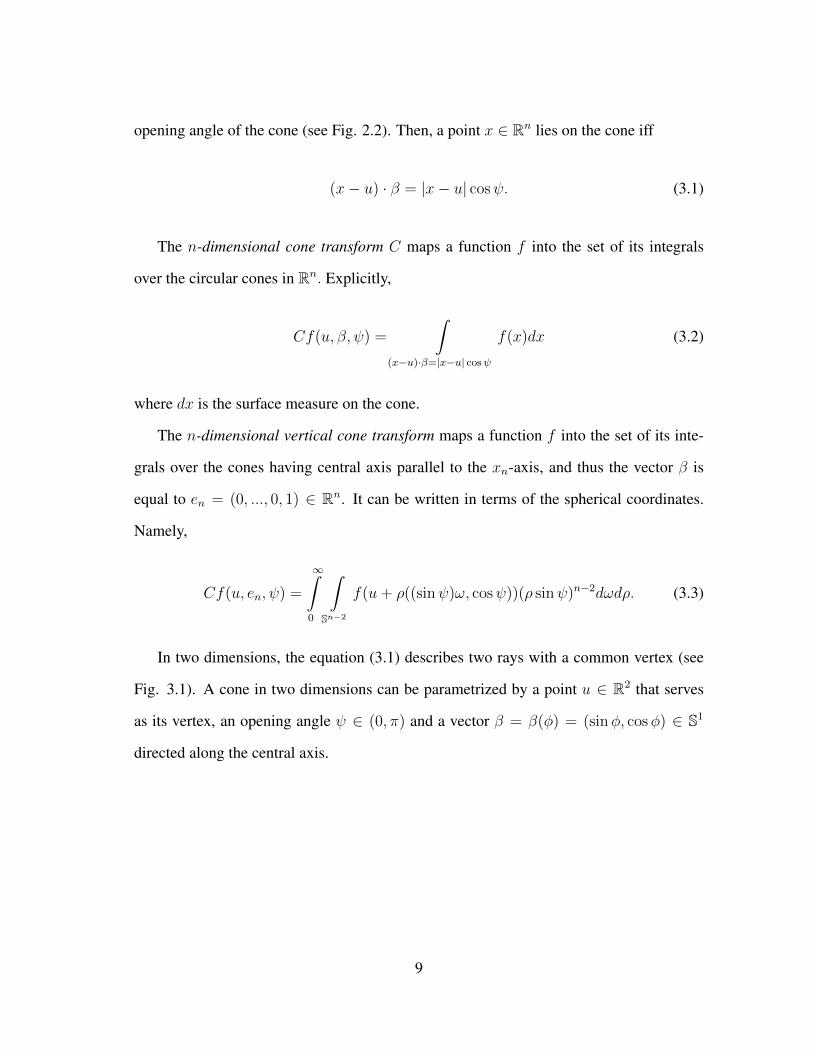
In two dimensions, the equation (3.1) describes two rays with a common vertex (see
Fig. 3.1). A cone in two dimensions can be parametrized by a point u ∈ R2 that serves
as its vertex, an opening angle ψ ∈ (0, π) and a vector β = β(φ) = (sinφ, cosφ) ∈ S1
directed along the central axis.
9

Figure 3.1: A Cone in 2-dimensions.
Then, the 2D cone transform of a function f ∈ S(R2) is given by
Cf(u, β, ψ) = Cf(u, β(φ), ψ) =
∞∫0
f(u+ r(sin(ψ + φ), cos(ψ + φ)))dr
+
∞∫0
f(u+ r(− sin(ψ − φ), cos(ψ − φ)))dr.
(3.4)
As a straightforward calculation shows, analogously to the Radon transform, cone
transform has an evenness property, and is shift and rotation invariant:
Lemma 3.1.1. Let f ∈ S(Rn), u ∈ Rn, β ∈ Sn−1 and ψ ∈ (0, π). Then,
1.
Cf(u,−β, ψ) = Cf(u, β, π − ψ). (3.5)
2. Let Ta be the translation operator in Rn, defined as Taf(x) = f(x+ a) for a ∈ Rn.
We define
Ta(Cf)(u, β, ψ) := Cf(u+ a, β, ψ).
10

Then,
TaC = CTa.
3. Let A be an n × n rotation matrix and MAf(x) = f(Ax) be the corresponding
rotation operator. We define
MA(Cf)(u, β, ψ) := Cf(Au,Aβ, ψ).
Then,
MAC = CMA.
3.2 Inversion of the Cone Transform
In the following, we investigate the relation between the cone and Radon transforms
and provide various analytic inversion formulas for the n-dimensional cone transform.
Theorem 3.2.1. Let f ∈ S(Rn). Then,
1. For any u ∈ Rn and β ∈ Sn−1, we have
π∫0
Cf(u, β, ψ)dψ =Γ(n−1
2)
2π(n−1)/2
∫Sn−1
Rf(ω, u · ω)dω =Γ(n−1
2)
2π(n−1)/2R#Rf(u), (3.6)
where R#, the dual operator to the Radon transform, is defined in Section B.2.
2. Let a function µ : Sn−1 → R be such that∫
Sn−1
µ(β)dβ = 1. Then,
f(x) =π−n/2Γ(n
2)
2Γ(n− 1)
∫Sn−1
π∫0
I1−nu→xCf(u, β, ψ)µ(β)dψdβ, (3.7)
where Iα is the Riesz potential defined in Section B.2.
11
Remark 3.2.2.
1. One notices that according to (3.6), the inversion formula (3.7) consists of a back-
projecting of the cone data, followed by a filtration (i.e., is what is called a FBP type
formula).
2. One can choose µ(β) to be equal to a delta-function, which would eliminate inte-
gration with respect to β in (3.7). However, if the signal is very week, eliminating
almost all values of β would lead to elimination of the signal. Thus weighted inte-
gration with respect to β allows for accounting for all data collected.
Proof. We first prove the theorem for dimensions n ≥ 3.
π∫0
Cf(u, en, ψ)dψ =
π∫0
∞∫0
∫Sn−2
f(u+ ρ((sinψ)ω, cosψ))(ρ sinψ)n−2dωdρdψ
=
∫Sn−1
∞∫0
f(u+ ρσ)ρn−2dρdσ =
∫Rn
f(u+ x)|x|−1dx =1
|Sn−2|R#Rf(u),
The last equality is due to [46, Chapter 2, Theorem 1.5] (see also (A.3)). As both R and
R# commute with rigid motions in Rn, we obtain for any β ∈ Sn−1,
π∫0
Cf(u, β, ψ)dψ =1
|Sn−2|R#Rf(u).
Thus, for any function µ on Sn−1 such that∫
Sn−1
µ(β)dβ = 1, we have
∫Sn−1
π∫0
Cf(u, β, ψ)µ(β)dψdβ =1
|Sn−2|R#Rf(u) =
Γ(n−12
)
2π(n−1)/2R#Rf(u).
12

Note that the last equality follows from the area formula for the n-sphere, that is
|Sn−1| = 2πn/2
Γ(n2). (3.8)
Using (B.16) with α = n− 1, and utilizing the gamma-function duplication formula (see
B.1.1)
Γ(z)Γ(z +1
2) = 21−2z√πΓ(2z), (3.9)
we conclude that
f(u) =πn/2Γ(n
2)
2Γ(n− 1)
∫Sn−1
π∫0
I1−nu→xCf(u, β, ψ)µ(β)dψdβ.
For the 2-dimensional case, we only need to provide the proof of (3.6), since the rest
of the proof stays the same. Assume for now that u = 0. By definition of the 2D cone
transform, we have
π∫0
Cf(0, β(φ), ψ)dψ =
π∫0
∞∫0
f(r sin(ψ + φ), r cos(ψ + φ))drdψ
+
π∫0
∞∫0
f(−r sin(ψ − φ), r cos(ψ − φ))drdψ.
Changing variables, we obtain
π∫0
f(r sin(ψ + φ), r cos(ψ + φ))dψ =
π+φ∫φ
f(r sinψ, r cosψ)dψ,
13
andπ∫
0
f(−r sin(ψ − φ), r cos(ψ − φ))dψ =
φ∫−π+φ
f(r sinψ, r cosψ)dψ.
Thus,
π∫0
Cf(0, β(φ), ψ)dψ =
∞∫0
π+φ∫−π+φ
f(r sinψ, r cosψ)dψdr.
Changing variables by letting θ =π
2− ψ and using 2π-periodicity of sine and cosine
functions, we get
π+φ∫−π+φ
f(r sinψ, r cosψ)dψ =
3π2−φ∫
−π2−φ
f(r cos θ, r sin θ)dθ =
2π∫0
f(r cos θ, r sin θ)dθ.
Therefore,
π∫0
Cf(0, β(φ), ψ)dψ =
2π∫0
∞∫0
f(r cos θ, r sin θ)drdθ =1
2
2π∫0
Rf(θ, 0)dθ,
where the last equality follows by letting n = 2 and p = 0 in (A.2). Now, using the shift
invariance of both cone and Radon transforms, we conclude that
π∫0
Cf(u, β, ψ)dψ =1
2
∫S1
Rf(ω, u · ω)dω =1
2R#Rf(u),
which is (3.6) with n = 2, so we are done.
Corollary 3.2.3. For n = 3, the formula (3.7) becomes
f(u) = − 1
4π
∫Sn−1
π∫0
∆Cf(u, β, ψ)µ(β)dψdβ,
14
where the Laplace operator ∆ acts in the variable u.
3.3 An Alternative Inversion Formula
For the derivation of an alternative inversion formula, we need the following relation
between the cone and Radon transforms.
Theorem 3.3.1. Let f ∈ S(Rn). For any u ∈ Rn and β ∈ Sn−1, we have
1
π
π∫0
Cf(u, β, ψ) sinψdψ =1
|Sn−1|
∫Sn−1
Rf(ω, ω · u)|ω · β|dω = C(R(Tuf))(β), (3.10)
where |Sn−1| denotes the area of the sphere Sn−1 and C is the cosine transform whose
definition is given in (B.26).
Proof. We first observe that if Duf(σ) :=
∞∫0
f(u+ ρσ)ρn−2dρ, then
F (Duf)(ω) =
∫Sn−1
Duf(σ)δ(ω · σ)dσ = Rf(ω, u · ω), (3.11)
where F denotes the Funk transform (see (B.21)). Indeed,
F (Duf)(ω) =
∫Sn−1
Duf(σ)δ(ω · σ)dσ
=
∫Sn−1
∞∫0
f(u+ ρσ)ρn−2dρδ(ω · σ)dσ
=
∫Sn−1
∞∫0
f(u+ ρσ)δ(ω · ρσ)ρn−1dρdσ
=
∫Rn
f(x)δ(ω · (x− u))dx = Rf(ω, u · ω).
15

It is known that S =π
|Sn−1|CF where S,C and F are the sine, cosine and Funk
transforms, respectively (see Appendix B.3 and [52, p. 284, (5.1.17)]). Applying cosine
transform and multiplying withπ
|Sn−1|in both sides of (3.11), we obtain
S(Duf) =π
|Sn−1|CF (Duf) =
π
|Sn−1|C(R(Tuf)).
That is,
∫Sn−1
Duf(σ)(1− (β · σ)2)1/2dσ =π
|Sn−1|
∫Sn−1
Rf(ω, u · ω)|β · ω|dω. (3.12)
It remains to show that
∫Sn−1
Duf(σ)(1− (β · σ)2)1/2dσ =
π∫0
Cf(u, β, ψ) sinψdψ. (3.13)
Since all S,C, D and R commute with rotations, it suffices to take β = en.
∫Sn−1
Duf(σ)(1− (en · σ)2)1/2dσ =
∫Sn−2
π∫0
Duf((sinψ)ω, cosψ)(sinψ)n−1dψdω
=
π∫0
∫Sn−2
∞∫0
f(u+ ρ(sinψ)ω, cosψ))(ρ sinψ)n−2dρdω sinψdψ
=
π∫0
Cf(u, en, ψ) sinψdψ.
An alternative proof of Theorem 3.3.1 is given in Appendix A.
The equality (3.10) enables us to invert the cone transform by utilizing the inversion
formulas for the Radon transform.
16

Theorem 3.3.2. Let f ∈ S(Rn). For any u ∈ Rn, we have
f(x) =Γ2(n+1
2)
2πnΓ(n)
∫Sn−1
π∫0
I1−nu→xCf(u, β, ψ) sinψdψdβ. (3.14)
Proof. Integrating both sides of (3.10) with respect to β over Sn−1, we obtain
∫Sn−1
π∫0
Cf(u, β, ψ) sinψdψdβ =π
|Sn−1|
∫Sn−1
Rf(ω, ω · u)
∫Sn−1
|ω · β|dβdω.
Using the rotation invariance of the Lebesgue measure on the sphere, for any ω ∈ Sn−1,
we compute
∫Sn−1
|ω · β|dβ =
∫Sn−2
π∫0
| cosφ|(sinφ)n−2dφdθ =2|Sn−2|n− 1
.
Thus, we get
∫Sn−1
π∫0
Cf(u, β, ψ) sinψdψdβ =π
|Sn−1|2|Sn−2|n− 1
∫Sn−1
Rf(ω, ω · u)dω
=2π
n− 1
|Sn−2||Sn−1|
∫Sn−1
R#Rf(u) =πΓ(n)
2n−1Γ2(n+12
)R#Rf(u). (3.15)
Note that, for the evaluation of the constant, we have used the area formula for the n-
sphere, (3.8) and the duplication formula (3.9). Now, using formula (B.16) with α = n−1,
we obtain the result.
Corollary 3.3.3. For n = 3, the formula (3.14) reads as
f(u) =−1
4π3
∫Sn−1
π∫0
∆Cf(u, β, ψ) sinψdψdβ,
17

where the Laplacian ∆ acts in the variable u.
3.4 Other Inversion Formulas
The main goal of this section is to derive a formula that is applicable in Compton
imaging (i.e., only uses the cone vertices located outside the object). The cosine transform
is a continuous bijection of C∞even(Sn−1) to itself (see e.g. [14], [52]). Since, for any f ∈
S(Rn), Rf(ω, 0) is an even function in C∞(Sn−1), we can recover the function R(Tuf)
explicitly for all u ∈ Rn by inverting the cosine transform according to the Theorem B.3.5.
Theorem 3.4.1. Let f ∈ S(Rn). For any u ∈ Rn and ω ∈ Sn−1, if n is even,
Rf(ω, ω · u) =−2n−1
Γ(n− 1)
π∫0
Pn/2(∆S)F (Cf)(u, ω, ψ) sinψdψ, (3.16)
and if n is odd,
Rf(ω, ω · u) =Γ(n+1
2)
π(n+1)/2
∫Sn−1
π∫0
Cf(u, β, ψ) sinψdψdβ (3.17)
− 2π−n/2
Γ(n2)P(n+1)/2(∆S)
∫
Sn−1
π∫0
Cf(u, β, ψ) log1
|ω · β|sinψdψdβ
,
where F is the Funk transform (B.21) and the operator Pr(∆S) is given in Theorem B.3.5,
both of them acting in the spherical variable ω.
Proof. The result follows by applying inverse cosine transform (B.27) and (B.28) to equal-
ity (3.10).
This result, in particular, answers the question of what geometries of Compton detec-
tors are sufficient for (stable) reconstruction of the function f . Indeed, formulas (3.17) and
(3.16) show that it is sufficient to have for any ω ∈ Sn−1 and s ∈ R a detector location u
such that ω · u = s. This can be rephrased in a nice geometric way:
18
Definition 3.4.2 (Compton Admissibility Condition). We will call an array of Compton de-
tectors admissible (for a given region of space), if any hyperplane intersecting this region,
intersects a detection site of the scattering detector.
So, if a set U of detectors is admissible for a region D ∈ Rn, then the formulas (3.17)
and (3.16) enable one to reconstruct the Radon transform of any function f supported
inside D, and thus f itself.
Here is a useful example of an application of the admissibility:
Proposition 3.4.3. Suppose that n = 3 and the detectors are placed on a sphere Sr of
radius r. We assume that the region for placing the object to be imaged is the concentric
sphere Sr′ of radius r′ = r − δ for some δ > 0. Then, any curve U on Sr that satisfies the
condition below is admissible:
Any circle on Sr of radius ρ ≥√δ(2r − δ) intersects U .
Proof. Indeed, every plane intersecting the interior of the sphere Sr′ intersect Sr over a
circle of radius ρ ≥√δ(2r − δ) and thus contains at least one detector.
Remark 3.4.4.
1. The experience of Radon transform shows that uniqueness of reconstruction should
hold for some non-admissible sets of detectors as well, although some (“invisible")
sharp details will get blurred in the reconstruction (see, e.g. [36, Ch. 7]). The
corresponding microlocal analysis of this issue will be done elsewhere.
2. The admissibility condition is not the minimal one. For instance, in the situation
of Proposition 3.4.3, the set of Compton data will still be 4-dimensional, and thus
somewhat overdetermined.
19

3. In the cases of low signal-to-noise ratio (e.g. SPECT and especially homeland se-
curity imaging), one would prefer to use larger admissible sets of detectors (e.g. 2D
rather than 1D arrays considered in Proposition 3.4.3), which would allow introduc-
ing additional (weighted, if needed) averaging, in order to reduce the effects of the
noise.
4. As it has been mentioned before, for all the reconstruction algorithms we develop in
this text, the geometry of detectors is irrelevant, as long as it satisfies the generous
Admissibility Condition 3.4.2 in section 2. If this condition is violated, one can
still use the algorithms, but then familiar limited data blurring artifacts [36, 46] will
appear.
A different approach to recovery of the Radon data from the Compton data comes from
the following known relation (see [19]) between the cosine and Funk transforms:
(∆S + n− 1)C = F, (3.18)
where ∆S is the Laplace-Beltrami operator on the unit sphere.
Indeed, applying (∆S + n− 1) to (3.10), we obtain
Φ(u, β) := F (R(Tuf))(β) =(∆S + n− 1)
π
π∫0
Cf(u, β, ψ) sinψdψ, (3.19)
where ∆S acts in variable β.
We now use the inversion formula for the Funk transform given in Theorem B.3.3 (see
also [52, Chapter 5, Theorem 5.37]), whose application to (3.19) leads to the following
result.
20
Theorem 3.4.5. Let f ∈ S(Rn), n ≥ 3. For any u ∈ Rn and ω ∈ Sn−1,
Rf(ω, ω · u) =Γ(n/2)
2πn/2
∫Sn−1
Φ(u, β)dβ (3.20)
+2n−1
(n− 2)!Q(∆S)
∫
Sn−1
Φ(u, β) log1
|ω · β|dβ
,
where
Q(∆S) = 4(1−n)/2(n−3)/2∏k=0
[−∆S + (2k + 1)(n− 3− 2k)] .
In particular, in 3D one arrives to
Corollary 3.4.6. For any u ∈ R3 and ω ∈ S2,
Rf(ω, ω · u) =1
4π
∫S2
Φ(u, β)dβ − ∆S
2π
∫S2
Φ(u, β) log1
|ω · β|dβ
. (3.21)
3.5 Reconstructions in Dimension Two
In 2D, for ω = (cos θ, sin θ), ∆S =∂2
∂θ2. Then the formula (3.16) reads as
Rf(ω, ω · u) =1
2(∂2
∂θ2+ 1)
π∫0
Cf(u, ω⊥, ψ) sinψdψ. (3.22)
We applied this approach to some 2D examples. Figures 3.2 and 3.3 show the recon-
structions of some phantoms from their projections collected by four Compton cameras
placed along the sides of a square. We simulate analytically the Compton projection data
of the phantoms and then use formula (3.16) to convert them to Radon projections. Fi-
nally, the filtered back-projection is applied to invert the Radon transform and obtain the
reconstructions.
21
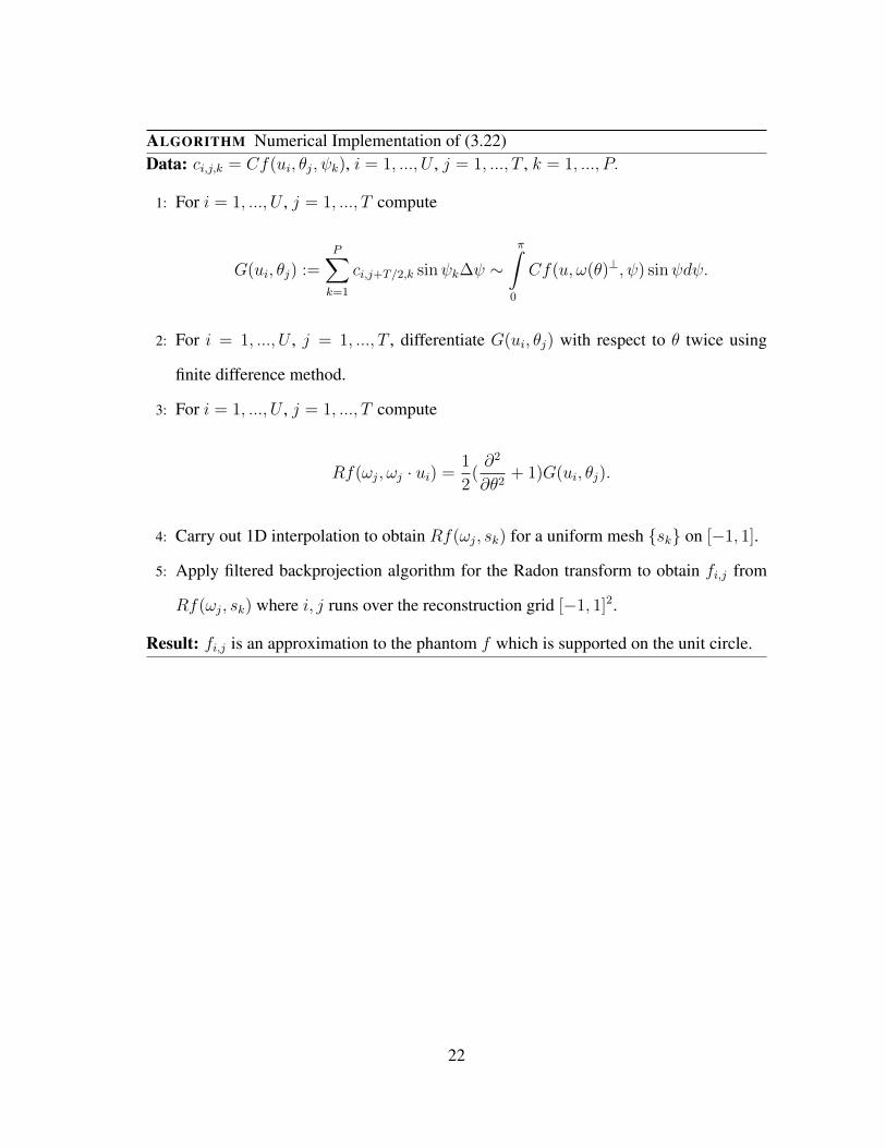
ALGORITHM Numerical Implementation of (3.22)Data: ci,j,k = Cf(ui, θj, ψk), i = 1, ..., U , j = 1, ..., T , k = 1, ..., P.
1: For i = 1, ..., U , j = 1, ..., T compute
G(ui, θj) :=P∑k=1
ci,j+T/2,k sinψk∆ψ ∼π∫
0
Cf(u, ω(θ)⊥, ψ) sinψdψ.
2: For i = 1, ..., U , j = 1, ..., T , differentiate G(ui, θj) with respect to θ twice using
finite difference method.
3: For i = 1, ..., U , j = 1, ..., T compute
Rf(ωj, ωj · ui) =1
2(∂2
∂θ2+ 1)G(ui, θj).
4: Carry out 1D interpolation to obtain Rf(ωj, sk) for a uniform mesh {sk} on [−1, 1].
5: Apply filtered backprojection algorithm for the Radon transform to obtain fi,j from
Rf(ωj, sk) where i, j runs over the reconstruction grid [−1, 1]2.
Result: fi,j is an approximation to the phantom f which is supported on the unit circle.
22

Figure 3.2: Left: The phantom is the characteristic function of a circle having density 1unit, radius 0.5 unit and centered at (0, 0). Right: 256x256 image reconstructed from thesimulated Compton data using 257 detectors per side and 200 counts for the angles β andψ each (see Fig. 3.1).
Figure 3.3: Left: The phantom is the sum of the characteristic functions of two intersectingcircles having densities 0.3 and 0.7 units, radii 0.5 and 0.3 units, and centered at (0, 0) and(0.5, 0). Right: 256x256 image reconstructed from the simulated Compton data using 257detectors per side and 200 counts for the angles β and ψ each (see Fig. 3.1).
23

3.6 Reconstructions in Dimension Three
In this section, we address the numerical implementation in the 3-dimensional case,
where we develop and apply three different inversion algorithms and study their feasibility.
Our first attempt has been to implement numerically the inversion formula (3.17) from
Theorem 3.4.1. The results were discouraging. The reason for this failure was that (3.17)
requires numerical computation of some singular integrals, followed then by applying to
the results a fourth order differential operator on the sphere.
Thus we had to resort to different inversion techniques, the description of which one
finds below.
In all examples below, the two-layer detectors cover the unit sphere S2 in R3 and the
object is located inside of this sphere and at some positive distance from it3. The algorithm
given in [50] is used to generate the triangular mesh on S2. The forward simulations of
Compton camera data were done numerically rather than analytically and thus involved
errors, which is in fact better for checking the validity and stability of the reconstruction
algorithms.
3.6.1 Method 1: Reconstruction Using Spherical Harmonics Expansions
In this section, we derive a series formula that recovers the Radon data from cone data.
Let us introduce the function
G(u, β) :=
π∫0
Cf(u, β, ψ) sinψdψ.
3The spherical geometry of the detector and of most of the phantoms we consider does not constitute anyinverse crime. This particular geometry is used to reduce immense computations of the synthetic forwarddata, which run for a long time even on multi-core machines. The inversion algorithms are not aware of thesymmetry of the detectors and/or phantoms.
24

For each fixed detector location u ∈ Rn, we can expand the function G(u, β) of β ∈ Sn−1
into spherical harmonics Y ml (see Appendix B.1.3):
G(u, β) =∞∑l=0
N(n,l)∑m=1
gml (u)Y ml (β), (3.23)
where
gml (u) =
∫Sn−1
G(u, β)Y ml (β)dβ
and
N(n, l) = (n+ 2l − 2)(n+ l − 3)!
l!(n− 2)!
(see e.g. [6, 45, 59]). Using (3.17), one obtains the following series inversion formula:
Theorem 3.6.1. For any u ∈ Rn and ω ∈ Sn−1,
Rf(ω, ω · u) =Γ(n+1
2)
πn/2g10(u)− 2π−n/2
Γ(n2)
∞∑l=1
dlqn,l
N(n,l)∑m=1
gml (u)Y ml (ω), (3.24)
where
qn,l = 4−(n+1)/2
(n−1)/2∏k=0
[l(l + n− 2) + (2k − 1)(n− 1− 2k)] (3.25)
and
dl = |Sn−2|1∫
−1
log1
|t|p(n−2)/2l (t)(1− t2)(n−3)/2dt, (3.26)
with p(n−2)/2l being the l-th degree Gegenbauer polynomial (see Appendix B.1.2).
25

Proof. Plugging (3.23) into the second term in the right hand side of (3.17), we obtain
Rf(ω, ω · u) =Γ(n+1
2)
2π(n+1)/2
∫Sn−1
G(u, β)dβ (3.27)
−2P(n+1)/2(∆S)
πn/2Γ(n2)
∞∑l=0
N(n,l)∑m=1
gml (u)
∫Sn−1
log1
|ω · β|Y ml (β)dβ.
We note that∫
Sn−1
G(u, β)dβ = 2√πg10(u). Then Funk-Hecke formula (see Theorem
B.1.1) implies that ∫Sn−1
log1
|ω · β|Y ml (β)dβ = dlY
ml (ω),
where dl is as in (3.26). Also, since ∆SYl = −l(l + n − 2)Yl, l = 0, 1, 2, ..., we have
P(n+1)/2(∆S)Yl = qn,lYl, where qn,l is given in (3.25). Hence, we get the result.
In particular, for n = 3, we get
Corollary 3.6.2. For any u ∈ R3 and ω ∈ S2,
Rf(ω, ω · u) = π−3/2g10(u)− 1
4π2
∞∑l=1
dlql
2l+1∑m=1
gml (u)Y ml (ω), (3.28)
where ql = (l − 1)l(l + 1)(l + 2) and dl = 2π
1∫−1
log1
|t|p(n−2)/2l (t)dt with p(n−2)/2l being
the l-th degree Gegenbauer polynomial (see Appendix B.1.2).
Remark 3.6.3. The coefficients ql in (3.28) are fourth order polynomials in l and account
for fourth order differentiation. Thus, it is expected to face an instability issue in the
numerical implementation of (3.28) when considering high degree spherical harmonics.
In our numerical tests, the phantom was the characteristic function of the 3D ball of
radius 0.5 centered at the origin, while the Compton detectors covered the concentric unit
26

sphere. The reason for considering a radial phantom is that its Radon transform can easily
be computed analytically. On the other hand, the Compton data was simulated numerically
and then used to numerically reconstruct the Radon data via (3.28). The results can then
be compared with the exact (analytically computed) Radon transforms4.
Figure 3.4 shows the comparison of the analytically computed Radon transform of
the phantom (shown in red) with its reconstructions, using (3.28). The results are illus-
trated for the direction ω = [−0.2342,−0.1844,−0.9545]. In obtaining the Radon data
Rf(ω, s) for uniformly sampled s ∈ [−1, 1] from Rf(ω, u · ω), we used MATLAB® tool-
box cftool with spline fitting having a smoothing parameter 0.99. The cone data is
numerically simulated for 1806 detector points on the sphere and 90 opening angles ψ.
For the cone axis direction vectors, we used varying discretization of the sphere corre-
sponding to 1806, 7446, and 30054 points. We have considered spherical harmonics up to
degree l = L = 30 in the expansion (3.23). In order to reduce the effect of instability, we
only used l = Lt in the computation of the Radon transform via (3.28) equal to 18.
4Tests on non-radial phantoms have lead to similar results.
27

ALGORITHM Numerical Implementation of (3.28)Data: ci,j,k = Cf(ui, βj, ψk), i = 1, ..., U , j = 1, ..., B, k = 1, ..., P.
1: For l = 1, ..., L, pre-compute
ql = (l − 1)l(l + 1)(l + 2) and dl ∼T∑i=1
p(n−2)/2l (ti)∆t
with p(n−2)/2l being the l-th degree Gegenbauer polynomial.
2: For i = 1, ..., U , j = 1, ..., B compute
G(ui, βj) :=P∑k=1
ci,j,k sinψk∆ψ ∼π∫
0
Cf(u, β, ψ) sinψdψ.
3: For i = 1, ..., U , and l = 1, ..., L, carry out the integral
gml (ui) =∑τ∈K
Area(τ)
3
∑v∈V (τ)
G(ui, v)Y ml (v) ∼
∫Sn−1
G(u, β)Y ml (β)dβ,
where m = 1, ..., 2l + 1, τ is a face of the triangular mesh K on S2, and V (τ) is the
set of vertices of τ .
4: For i = 1, ..., U , j = 1, ..., T , and ωj ∈ K, a triangular mesh on S2, compute
Rf(ωj, ωj · ui) = π−3/2g10(u)− 1
4π2
Lt∑l=1
dlql
2l+1∑m=1
gml (ui)Yml (ωj).
5: Carry out 1D interpolation to obtain Rf(ωj, sk) for a uniform mesh {sk} on [−1, 1].
6: Apply filtered backprojection algorithm for the Radon transform to obtain fi,j,l from
Rf(ωj, sk) where i, j, l runs over the reconstruction grid [−1, 1]3.
Result: fi,j,l is an approximation to the phantom f which is supported on the unit sphere.
28
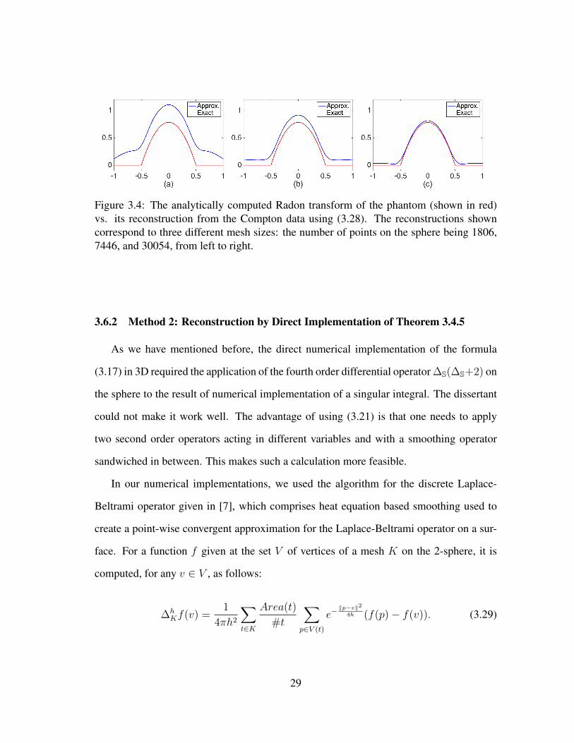
Figure 3.4: The analytically computed Radon transform of the phantom (shown in red)vs. its reconstruction from the Compton data using (3.28). The reconstructions showncorrespond to three different mesh sizes: the number of points on the sphere being 1806,7446, and 30054, from left to right.
3.6.2 Method 2: Reconstruction by Direct Implementation of Theorem 3.4.5
As we have mentioned before, the direct numerical implementation of the formula
(3.17) in 3D required the application of the fourth order differential operator ∆S(∆S+2) on
the sphere to the result of numerical implementation of a singular integral. The dissertant
could not make it work well. The advantage of using (3.21) is that one needs to apply
two second order operators acting in different variables and with a smoothing operator
sandwiched in between. This makes such a calculation more feasible.
In our numerical implementations, we used the algorithm for the discrete Laplace-
Beltrami operator given in [7], which comprises heat equation based smoothing used to
create a point-wise convergent approximation for the Laplace-Beltrami operator on a sur-
face. For a function f given at the set V of vertices of a mesh K on the 2-sphere, it is
computed, for any v ∈ V , as follows:
∆hKf(v) =
1
4πh2
∑t∈K
Area(t)
#t
∑p∈V (t)
e−‖p−v‖2
4h (f(p)− f(v)). (3.29)
29

Here, for any face t ∈ K, the number of vertices in t is denoted by #t, and V (t) is the
set of vertices of t. The parameter h is a positive quantity (akin to the time in the heat
equation), which intuitively corresponds to the size of the neighborhood considered at
each point. The authors of [7] suggest that h can be taken to be a function of v, which
allows the algorithm to adapt to the local mesh size.
In our experiments, we used the adaptive parameter h(v) = 0.0156×(the average
edge length at v). We used the same phantom as in the previous section. Figure 3.5
shows the comparison of the analytically computed Radon transform of the phantom
(shown in red) with its reconstructions. The results are illustrated for the direction ω =
[−0.2363,−0.2484,−0.9394]. In obtaining the Radon data for uniformly sampled s ∈
[−1, 1] from Rf(ω, u · ω), we used the same MATLAB® toolbox cftool with spline
fitting having a smoothing parameter 0.995. The cone data is numerically simulated for
1806 detector points on the sphere and 90 opening angles ψ. For the cone axis direction
vectors, we used varying discretization of the sphere corresponding to 1806, 7446, and
30054 points.
30

ALGORITHM Numerical Implementation of (3.20)Data: ci,j,k = Cf(ui, βj, ψk), i = 1, ..., U , j = 1, ..., B, k = 1, ..., P.
1: For i = 1, ..., U , j = 1, ..., B compute
G(ui, βj) :=P∑k=1
ci,j,k sinψk∆ψ ∼π∫
0
Cf(u, β, ψ) sinψdψ.
2: For i = 1, ..., U , and l = 1, ..., L, apply discrete Laplace-Beltrami operator (3.29) in
β to G(ui, βj).
3: For i = 1, ..., U , j = 1, ..., T , compute Φ(ui, βj) as in (3.19).
4: For i = 1, ..., U , and l = 1, ..., L, carry out the integrals
∫Sn−1
Φ(u, β)dβ ∼∑τ∈K
Area(τ)
3
∑v∈V (τ)
Φ(ui, v)
and, for ωj ∈ K, a triangular mesh on S2,
∫Sn−1
Φ(u, β) log1
|ω · β|dβ ∼
∑τ∈K
Area(τ)
3
∑v∈V (τ)
Φ(ui, v) log1
|ωj · v|.
where τ is a face of the triangular mesh K on S2, and V (τ) is the set of vertices of τ .
5: Using the results of the previous step, compute Rf(ωj, ωj · ui) as in (3.20).
6: Carry out 1D interpolation to obtain Rf(ωj, sk) for a uniform mesh {sk} on [−1, 1].
7: Apply filtered backprojection algorithm for the Radon transform to obtain fi,j,l from
Rf(ωj, sk) where i, j, l runs over the reconstruction grid [−1, 1]3.
Result: fi,j,l is an approximation to the phantom f which is supported on the unit sphere.
31

Figure 3.5: The Radon transform of the phantom recovered using (3.21) and (3.29). Thereconstructions shown corresponds to three different mesh sizes: the number of points onthe sphere being 1806, 7446, and 30054, from left to right.
3.6.3 Method 3: Reconstruction via a Mollified Inversion of the Cosine Transform
The formula (3.10) shows that availability of any cosine transform inversion would
also lead to an inversion of the cone transform, and such approximate and exact inversions
of C indeed exist [40,51,52]. We apply here the method of approximate inverse developed
in [39, 40, 51], which is an incarnation of a general approach to solving inverse problems
numerically. Namely, for a given data h, the aim is to find g satisfying Cg = h. If we find
a ‘Green’s function’ ψ such that Cψ = δ, then the spherical convolution h ∗ ψ of h and
ψ solves the equation Cg = h. Now, if one picks a ‘mollifier’ (an approximation to the
δ-function) δγ and “approximate Greens function” ψγ , such that Cψγ = δγ , then one finds
the approximate solution gγ = g ∗ δγ .
In our numerical tests, we used the reconstruction kernel ψγ that was analytically com-
puted in [51] for a special class of mollifiers (see [51, (4.1) and (4.10)]). We used the same
phantom as in the previous sections. Figure 3.6 shows the comparison of the analytically
computed Radon transform of the phantom (shown in red) with its reconstructions, using
(3.28). The results are illustrated for the direction ω = [−0.2342,−0.1844,−0.9545]. The
MATLAB® toolbox cftool was used with the smoothing parameter 0.99999999. The
32

cone data is numerically simulated for 1806 detector points on the sphere and 90 opening
angles ψ. For the cone axis direction vectors, we used varying discretization of the sphere
corresponding to 1806, 7446, and 30054 points.
ALGORITHM Reconstruction via a mollified inversion of the Cosine TransformData: ci,j,k = Cf(ui, βj, ψk), i = 1, ..., U , j = 1, ..., B, k = 1, ..., P.
1: For i = 1, ..., U , j = 1, ..., B compute
G(ui, βj) :=P∑k=1
ci,j,k sinψk∆ψ ∼π∫
0
Cf(u, β, ψ) sinψdψ.
2: For i = 1, ..., U , and for ωl ∈ K, a triangular mesh on S2, compute
Rf(ωl, ωl · ui) = 4∑τ∈K
Area(τ)
3
∑v∈V (τ)
G(ui, v)ψγ(ωl · v) ∼ 4
∫Sn−1
G(u, β)ψγ(ω · β)dβ.
where ψγ is given as in [51, Theorem 4.7], and τ is a face of the triangular mesh K on
S2, and V (τ) is the set of vertices of τ .
3: Carry out 1D interpolation to obtain Rf(ωl, sk) for a uniform mesh {sk} on [−1, 1].
4: Apply filtered backprojection algorithm for the Radon transform to obtain fi,j,l from
Rf(ωl, sk) where i, j, l runs over the reconstruction grid [−1, 1]3.
Result: fi,j,l is an approximation to the phantom f which is supported on the unit sphere.
33

Figure 3.6: The Radon transform of the phantom using the method of mollified inversefor the cosine transform. The reconstructions shown corresponds to three different meshsizes: the number of points on the sphere being 1806, 7446, and 30054, from left to right.
One notices insufficient resolution of singularity, which is due to the insufficiently fine
approximation of δ-function by δγ chosen in [40, 51].
3.6.4 Comparison of the Three Methods
While above we only addressed reconstructing the Radon transform of the function
in question, here we show how the three methods perform after taking the final step of
inverting the Radon transform and reconstructing the characteristic function of the ball.
The inversion of Radon transform from the reconstructed values Rf(ω, s) was done
according to the formula (B.16) with α = 0. We used 128 values of s and 480 directions ω
in methods 1 and 3, and 1806 directions in method 2. We used the filtered backprojection
formula with the filter given in [41]. The normalized L2 and H1 errors for the Radon
transforms obtained in each of the methods are summarized in Table 3.1. The reason for
considering the H1-error is the fact that H1-norm control of the 3D Radon transform data
Rf corresponds to the L2-norm control of the tomogram f [46].
34

Method L2 Error H1 Error
1 0.0986 0.3231
2 0.1046 0.3767
3 0.0896 0.3660
Table 3.1: The normalized L2 and H1 errors for the Radon data for each of the threemethods.
Figure 3.7 shows the three cross-sections of the spherical phantom and of its recon-
structions from the Radon data obtained via the three methods above. The finest mesh on
the sphere (30054 points) was used.
35
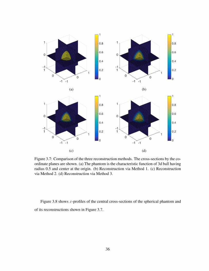
(a) (b)
(c) (d)
Figure 3.7: Comparison of the three reconstruction methods. The cross-sections by the co-ordinate planes are shown. (a) The phantom is the characteristic function of 3d ball havingradius 0.5 and center at the origin. (b) Reconstruction via Method 1. (c) Reconstructionvia Method 2. (d) Reconstruction via Method 3.
Figure 3.8 shows x-profiles of the central cross-sections of the spherical phantom and
of its reconstructions shown in Figure 3.7.
36

Figure 3.8: x-profiles of the phantom and the reconstructions in Figure 3.7, (a) method 1,(b) method 2 and (c) method 3.
It is important to note that in all of the methods, there are parameters that can still
be optimized, namely L and Lt in Method 1, h in Method 2, and γ and ν in Method 3
(see [51]).
We have also tested the reaction of our algorithms to random noise. The 20% Gaussian
white noise added to the cone data for Methods 1 and 2. For Method 2, we added 10%
noise to the cone data. Figure 3.9 shows the three cross-sections of the spherical phantom
and of its reconstructions from the Radon data obtained via the three methods above. The
finest mesh on the sphere (30054 points) was used.
37

(a) (b)
(c) (d)
Figure 3.9: Comparison of the three reconstruction methods. The cross-sections by thecoordinate planes are shown. (a) The phantom is the characteristic function of 3d ballhaving radius 0.5 and center at the origin. (b) Reconstruction via Method 1 from datacontaminated with 20% Gaussian white noise. (c) Reconstruction via Method 2 from datacontaminated with 10% Gaussian white noise. (d) Reconstruction via Method 3 from noisydata contaminated with 20% Gaussian white noise.
Figure 3.10 shows x-profiles of the central cross-sections of the spherical phantom and
of its reconstructions shown in Figure 3.9.
38

Figure 3.10: Comparison of x-profiles of central slices of phantom and the reconstructionsfrom noisy data shown in Figure 3.9.
39

4. INVERSION OF WEIGHTED DIVERGENT BEAM AND CONE
TRANSFORMS1
In this chapter, we consider the weighted divergent beam and cone transforms, and
discuss their inversion. In Section 4.1, we define the weighted divergent beam and cone
transforms and describe a simple relation between them. In Section 4.2, we present a vari-
ety of inversion formulas for the weighted divergent beam transform (Theorems 4.2.5 and
4.2.7). We then derive an integral relation between the weighted divergent beam and cone
transforms in Section 4.3, which leads to new inversion formulas for the n-dimensional
weighted cone transform (Theorem 4.3.6). In Section 4.4, we investigate the relation be-
tween the Radon and weighted divergent beam and cone transforms. This enables us to
derive other inversion formulas for the latter two (Theorem 4.4.4). Section 4.5 contains the
results of numerical implementation of some of the inversion formulas for the weighted
cone transform in dimensions two and three for two different vertex geometries, as well as
examples of numerical inversion of two weighted divergent beam transforms in dimension
three.
4.1 The Weighted Cone and Divergent Beam Transforms
In this section, we define the closely related weighted divergent beam and cone trans-
forms.
Definition 4.1.1. For k > −1, the k-weighted divergent beam transform of a function1Reprinted from: Inversion of weighted divergent beam and cone transforms, by P. Kuchment and F.
Terzioglu, Inverse Problems & Imaging, Volume 11, 2017. Copyright © by AIMS. Reprinted with thepermission of AIMS.
40

f ∈ S(Rn) is defined by
Dkf(u, σ) = Dkuf(σ) :=
∫ ∞0
f(u+ ρσ)ρkdρ, (4.1)
where u ∈ Rn is the source of the beam {u + ρσ}|ρ≥0 and σ ∈ Sn−1 is the unit vector in
the direction of the beam.
Consider now a circular cone2 S in Rn. The set of such cones can be parametrized by
a triple (u, β, ψ), where u ∈ Rn is the cone’s vertex (apex)3, the unit vector β ∈ Sn−1 is
directed toward cone’s interior along the cone’s axis, and ψ ∈ (0, π) is the opening angle
(see Fig. 4.1). A point x ∈ Rn lies on S(u, β, ψ) iff (x− u) · β = |x− u| cosψ.
Figure 4.1: A cone with vertex u ∈ Rn, central axis direction vector β ∈ Sn−1 and openingangle ψ ∈ (0, π).
Definition 4.1.2. Let k ∈ Z+ = {0, 1, 2, ...}, and suppose that f ∈ S(Rn). We define the
2The word “cone” in this paper always means a surface, rather than solid cone.3In the Compton camera imaging, cone’s vertex corresponds to a detection location.
41

k-weighted cone transform Ckf of f as
Ckf(u, β, ψ) :=
∫S(u,β,ψ)
f(x)|x− u|k−n+2dS(x), (4.2)
where dS is the surface measure on the cone S. In other words,
Ckf(u, β, ψ) = sinψ
∫Rnf(x)δ((x− u) · β − |x− u| cosψ)|x− u|k−n+2dx, (4.3)
where dx is the Lebesgue measure on Rn.
Remark 4.1.3.
• To avoid confusion, note that the power in the integral weight in the definition of
Ckf is not equal to k, but rather also depends on the spatial dimension n.
• At this step, one can allow all real values k > −1, while later on, k ∈ Z+ :=
{0, 1, 2, . . . } will be important.
• We note that k = n−2 corresponds to the case of pure surface measure on the cone.
Remark 4.1.4. We will say just “weighted" cone or divergent beam transform, when no
confusion about the value of k can arise.
Changing variables in (4.3) as x = u+ ρσ for ρ ∈ [0,∞) and σ ∈ Sn−1, and using the
fact that δ is homogeneous of degree −1, we make the following simple observation:
Proposition 4.1.5. Let u ∈ Rn, β ∈ Sn−1 and ψ ∈ (0, π). Then,
Ckf(u, β, ψ) = sinψ
∫Sn−1
∫ ∞0
f(u+ ρσ)ρkdρ δ(σ · β − cosψ)dσ
= sinψ
∫Sn−1
Dkuf(σ)δ(σ · β − cosψ)dσ. (4.4)
42

By letting t = cosψ, we can rewrite (with an abuse of notation) Ckf as
Ckf(u, β, t) :=
√
1− t2∫Sn−1
Dkuf(σ)δ(σ · β − t)dσ, if |t| ≤ 1
0, otherwise.
(4.5)
4.2 Inversion of the Weighted Divergent Beam Transform
If f ∈ S(Rn), for each u ∈ Rn,Dkuf(σ) can be uniquely extended to a smooth function
on Rn\{0} homogeneous of degree −(k + 1):
Dkuf(x) =
1
|x|k+1Dkuf(
x
|x|). (4.6)
This function is locally integrable with respect to x ∈ Rn, provided k < n − 1, and has
a well-defined Fourier transform as a tempered distribution (see e.g. [17]), i.e., for each
ϕ ∈ S(Rn),
〈Dkuf(ξ), ϕ(ξ)〉 =
∫RnDkuf(y)ϕ(y)dy. (4.7)
In the following, we derive inversion formulas for the divergent beam transform that are
analogs of the well known [63,64] Tuy’s inversion formula, which addresses the case when
k = 0 in dimension three, and the sources (detectors in the Compton camera case) move
along a curve.
In the rest of the paper, the shorthand notations ∂uj and ∂u will be used for the partial
derivatives ∂/∂uj and gradient∇u with respect to the variables u.
Theorem 4.2.1. Let k ∈ Z+, f ∈ S(Rn), and all source locations u are accessible. Then,
f(x) =(−i)k+1
(2π)n
∫Sn−1
(∆(k+1)/2u Dk
uf(θ)) ∣∣
u=xdθ, (4.8)
43

where ∆u :=∑
j ∂2uj
is the Laplace operator with respect to the variable u, and its power
when k is not an odd integer is understood as the corresponding Riesz potential (see,
e.g. [46]).
Proof. Let f ∈ S(Rn). For any θ ∈ Sn−1, the Fourier transform of Dkuf satisfies
Dkuf(θ) =
∫ ∞0
eiρθ·uf(ρθ)ρn−k−2dρ. (4.9)
Indeed, for any ϕ ∈ S(Rn), due to Dkuf being homogeneous of degree −(k + 1) and
changing to polar variables y = sω, we have
〈Dkuf, ϕ〉 = 〈Dk
uf, ϕ〉 =
∫RnDkuf(y)ϕ(y)dy
=
∫Sn−1
∫ ∞0
Dkuf(ω)ϕ(sω)sn−k−2dsdω
=
∫Rnϕ(x)
∫Sn−1
∫ ∞0
∫ ∞0
e−ix·sωf(u+ rω)sn−k−2ds rkdrdω dx.
Now, changing variables in s to ρ = s/r, and then letting y = u+ rω, we get
〈Dkuf, ϕ〉 =
∫Rnϕ(x)
∫ ∞0
∫Sn−1
∫ ∞0
e−ix·rρωf(u+ rω)rn−1drdωρn−k−2dρ dx
=
∫Rnϕ(x)
∫ ∞0
∫Rne−iρx·(y−u)f(y)dyρn−k−2dρ dx,
which implies (4.9).
The following simple formula holds for any unit vector θ:
∆(k+1)/2u eiρθ·u = (iρ)k+1eiρθ·u. (4.10)
Thus, applying (k+1)/2-th power of the Laplace operator with respect to u to (4.9), we
44

obtain
∆(k+1)/2u Dk
uf(θ) = ik+1
∫ ∞0
eiρθ·uf(ρθ)ρn−1dρ. (4.11)
Now, recalling the Fourier inversion formula in polar coordinates
f(x) =1
(2π)n
∫Sn−1
∫ ∞0
eiρθ·xf(ρθ)ρn−1dρdθ (4.12)
and comparing with (4.11), we obtain the desired formula
f(x) =(−i)k+1
(2π)n
∫Sn−1
(∆(k+1)/2u Dk
uf(θ)) ∣∣
u=xdθ.
Remark 4.2.2. Considering formula (4.8), one realizes quickly that it is not very useful,
since it requires “sources” u of the beams to be available throughout the whole space. In
the Compton camera case, as well as in 3D CT, this would require detectors/sources to be
placed throughout the object imaged, which is impossible.
Moreover, in this case, one deals with just a deconvolution problem, and a severely
overdetermined one at that (the dimension of the data used is 2n − 1 instead of n). Thus,
there must exist formulas requiring much less data, in particular allowing the detectors u
to be situated only outside the object being imaged (e.g. Tuy’s formula only requires an
arc of external sources).
This is also related to the interesting question about “admissible” complexes of cones
that provide enough data for stable reconstruction. We have already briefly addressed this
issue in [37, 60] and plan to have more detailed discussion elsewhere.
Here we show an example of how such deficiency can be alleviated for the weighted
45

divergent beam transform.
Definition 4.2.3.
• LetM ⊂ Rn be a smooth d-dimensional submanifold. We will say that it satisfies
the Tuy’s condition with respect to a subset V ⊂ Rn, if any hyperplane intersecting
V has a non-tangential intersection withM.
Equivalently: for any x ∈ V and unit vector θ ∈ Sn−1, there exists a point u ∈ M
such that θ · x = θ · u, and θ is not normal toM at the point u.
• We denote by Pu the orthogonal projection onto the tangent space toM at the point
u ∈M.
Remark 4.2.4. Notice that the above condition is a strengthened version of what was
called admissibility condition in [37, 60].
Theorem 4.2.5. Let k be an odd non-negative integer andM ⊂ Rn satisfies Tuy’s con-
dition with respect to a compact V . Then, for any homogeneous linear elliptic differential
operator L(u, ∂u) of order k + 1 on M and any smooth function f supported in V , the
following inversion formula holds:
f(x) =1
(2π)n
∫Sn−1
1
L(u, Puθ)L(u, ∂u)Dk
uf(θ)dθ, (4.13)
where u ∈M is related to x and θ as in the Tuy’s condition.
IfM is one-dimensional, then k can be any natural number (in this case, when k = 0,
one ends up with the standard Tuy’s formula).
Remark 4.2.6.
• Notice that u ∈ M in (4.13) depends on both x and θ and that L(u, Puθ) does not
vanish if the Tuy’s condition is satisfied.
46

• The differential expression in the formula above is written in the variable u, while
the actual variables at hand are θ and x. Due to the non-tangentiality required in
the Tuy’s condition, such a differential operator can be locally lifted to an opera-
tor in (x, θ) variables (which requires a specific calculation for each manifold of
detectors).
• The choice of u in Tuy’s condition might not be unique, and any such choice will
work.
Proof. The proof follows exactly the one of Theorem 4.2.1, using at the end the formula
for the symbol of a homogeneous differential operator of order k + 1 (instead of a power
of the Laplacian in (4.10)):
L(u, ∂u)eiρθ·u = (iρ)k+1L(u, Puθ)e
iρθ·u (4.14)
and noticing that the factor L(u, Puθ) does not vanish, due to the ellipticity and homo-
geneity of the operator and the Tuy’s condition.
A serious deficiency in Theorem 4.2.5 is that, unlessM is one-dimensional, only odd
values of k are allowed. This issue can be resolved, paying the price of having a more
complex formula.
Indeed, consider the following first order linear differential operator acting tangentially
toM, with coefficients depending upon u ∈M and θ ∈ Sn−1:
O(u, θ, ∂u) := Puθ · ∂u. (4.15)
Let also L(u, ∂u) be an operator like in Theorem 4.2.5, but of order k. Applying the
composition O ◦ (aL) to the exponential eiρθ·u, where a := 1/L(u, Puθ), and using (4.14),
47

we get
O ◦ (aL)eiρθ·u = |Puθ|2(iρ)k+1eiρθ·u. (4.16)
Since the order of the composition is odd, this enables us to extended the inversion formula
to the even values of k:
Theorem 4.2.7. Let k be an even non-negative integer andM⊂ Rn satisfies Tuy’s condi-
tion with respect to a compact V . Then, for any homogeneous elliptic differential operator
L(u, ∂u) of order k onM and any smooth function f supported in V , the following inver-
sion formula holds:
f(x) =1
(2π)n
∫Sn−1
1
|Puθ|2(O ◦ 1
L(u, Puθ)L)Dkuf(θ)dθ, (4.17)
where u is related to x and θ as in the Tuy’s condition.
Proof. The proof stays exactly the same, except instead of (4.14), we use (4.16).
Remark 4.2.8. Since we are dealing with a severely overdetermined transform, the vari-
ety of possible inversion formulas is large and is not exhausted by the ones above. For
instance, instead of using the operator 1|Puθ|2 (O ◦ 1
L(u,Puθ)L), one can use ( 1
|Puθ|2O)k+1.
4.3 Inversion of the Weighted Cone Transform
The following result presents a relation between the weighted divergent beam and cone
transforms defined in section 4.1, which will be instrumental in the inversion of the latter
one.
Proposition 4.3.1. Suppose that f ∈ S(Rn), and h(t) is a distribution on R regular near
t = ±1. Then,
⟨h(t),
Ckf(u, β, t)√1− t2
⟩R = 〈h(σ · β), Dk
uf(σ)〉Sn−1 . (4.18)
48
(Notice that Ckf(u, β, t) = 0 for |t| > 1, and is smooth for |t| < 1.)
Proof. By the representation (4.5) of the weighted cone transform, we have
⟨h(t),
Ckf(u, β, t)√1− t2
⟩R =
⟨h(t), 〈δ(σ · β − t), Dk
uf(σ)〉Sn−1
⟩R
=⟨(h ∗ δ)(σ · β), Dk
uf(σ)⟩Sn−1 = 〈h(σ · β), Dk
uf(σ)〉Sn−1 .
We note that (4.18) is equivalent to
∫ π
0
Ckf(u, β, ψ)h(cosψ)dψ =
∫Sn−1
Dkuf(σ)h(σ · β)dσ. (4.19)
Definition 4.3.2. Let k < n− 1. We introduce the following distribution:
hn,k(t) :=
∫ ∞0
e−itssn−k−2ds (4.20)
= in−k−1[(n− k − 2)!tk−n+1 + (−1)n−k−1iπδ(n−k−2)(t)],
(see e.g. [17, Chapter 2, p.172, eqn. (5)]).
Proposition 4.3.3. The following identity holds:
Dkuf(ξ) =
∫Sn−1
Dkuf(σ)hn,k(σ · ξ)dσ. (4.21)
49
Proof. For each ϕ ∈ S(Rn), since Dkuf is homogeneous of degree −(k + 1), we have
〈Dkuf, ϕ〉 = 〈Dk
uf, ϕ〉 =
∫RnDkuf(y)ϕ(y)dy
=
∫Sn−1
∫ ∞0
Dkuf(σ)ϕ(sσ)sn−k−2dsdσ
=
∫Sn−1
∫ ∞0
Dkuf(σ)
∫Rne−isσ·ξϕ(ξ)dξsn−k−2dsdσ
=
∫Rn
∫Sn−1
Dkuf(σ)hn,k(σ · ξ)dσϕ(ξ)dξ,
which implies (4.21).
Now, by combining (4.19) and (4.21), and using the inversion formula for the weighted
divergent beam transform (4.8), we obtain an inversion formula for the weighted cone
transform.
Theorem 4.3.4. Let f ∈ S(Rn), and k < n− 1. Then,
f(x) =(−i)k+1
(2π)n
∫Sn−1
∫ π
0
(∆(k+1)/2u Ckf(u, β, ψ)
)∣∣u=x
hn,k(cosψ)dψdβ. (4.22)
Remark 4.3.5. The same deficiency applies here that was mentioned in remark 4.2.2: the
formula requires the cones to be available with all vertices u throughout the space, which
is unacceptable for many imaging applications (e.g. Compton ones). Fortunately, a similar
remedy as for the divergent beam transform exists, which we address next.
Theorem 4.3.6. Let k ∈ Z+, k < n − 1. Suppose that M ⊂ Rn satisfies the Tuy’s
condition with respect to a compact V ⊂ Rn, and f is a smooth function supported in V .
Then, depending on the parity of k, the following inversion formulas hold:
1. if k is odd, then for any homogeneous linear elliptic differential operator L(u, ∂u) of
50
order k + 1 onM
f(x) =1
(2π)n
∫Sn−1
∫ π
0
1
L(u, Puθ)L(u, ∂u)C
kf(u, θ, ψ)hn,k(cosψ)dψdθ, (4.23)
2. if k is even, then for any homogeneous linear elliptic differential operator L(u, ∂u)
of order k onM
f(x) =1
(2π)n
∫Sn−1
∫ π
0
1
|Puθ|2(O ◦ 1
L(u, Puθ)L)Ckf(u, θ, ψ)hn,k(cosψ)dψdθ,
(4.24)
where O is given as in (4.15), and u ∈ M is related to x and θ as in the Tuy’s
condition.
Proof. The proof is just an immediate consequence of the equalities (4.21), (4.19), (4.13),
and (4.17) (in that order).
4.4 Relations with the Radon Transform: Other Inversion Formulas
In this section, we first present a relation between the Radon and the weighted divergent
beam and cone transforms for any dimension n and any k ∈ Z+. Analogous relation for
the usual divergent beam transform (k = 0) is obtained in [25] (see also [64, Chapter 2]).
Proposition 4.4.1. Let f ∈ S(Rn) and h be a distribution on R which is homogeneous of
degree k − n+ 1 and regular around ±1. Then,
∫ π
0
Ckf(u, β, ψ)h(− cosψ)dψ (4.25)
=
∫Sn−1
Dkuf(σ)h(−σ · β)dσ =
∫RRf(β, s)h(u · β − s)ds = (Rβf ∗ h)(u · β).
Proof. The first equality is already obtained in Proposition 4.3.1. By definition of the
51

weighted divergent beam transform, we have
∫Sn−1
Dkuf(σ)h(−σ · β)dσ =
∫Sn−1
∫ ∞0
f(u+ ρσ)ρkdρh(−σ · β)dσ
=
∫Sn−1
∫ ∞0
f(u+ ρσ)h(−ρσ · β)ρn−1dρdσ,
due to the homogeneity of h. Letting x = u+ ρσ, we obtain
∫Sn−1
∫ ∞0
f(u+ ρσ)h(−ρσ · β)ρn−1dρdσ
=
∫Rnf(x)h((u− x) · β)dx =
∫Rnf(x)
(∫Rh(u · β − s)δ(x · β − s)ds
)dx
=
∫R
(∫Rnf(x)δ(x · β − s)dx
)h(u · β − s)ds =
∫RRf(β, s)h(u · β − s)ds.
Remark 4.4.2. In dimensions two and three, for k = 0 and k = 1, respectively, the
relation (4.25) gives the following (geometrically obvious) formula:
Ckf(u, β,π
2) = R(β, u · β),
which is used in [6] in dimension three.
Remark 4.4.3. In dimension three, a special case of (4.25), namely for h(t) = tk−2, is
proven and used to derive an inversion formula for the cone transform for k = 0 and k = 1
in [57]. In dimension two, an inversion formula for k = 0 is derived using (4.25) with
h(t) = t−1 in [1, 18]. For the usual divergent beam transform (k = 0) in dimension three,
the applications of various functions h can be found in [64, Chapter 2, and references
therein].
52
Let k ∈ Z+, and h be the function on R defined by
h(t) :=
1
2(k − n+ 1)!|t|k−n+1sgn t, if k > n− 2 and k − n is odd,
1
2(k − n+ 1)!|t|k−n+1, if k > n− 2 and k − n is even,
δ(n−k−2)(t), if k ≤ n− 2.
(4.26)
We note that h is homogeneous of degree k−n+1, and for k > n−2, h(k−n+2) = δ(t)
(see e.g. [17]).
Now, using the differentiation property of the convolution
∂α(g ∗ h) = ∂αg ∗ h = g ∗ ∂αh
and the inversion formula (B.18) for the Radon transform, we obtain the following for-
mula, which can be used for inversion of both the weighted divergent beam and cone
transforms:
Theorem 4.4.4. Suppose that for any u ∈M and β ∈ Sn−1, s = u · β and
G(β, s) := (Rβf ∗ h)(s) =
∫ π
0
Ckf(u, β, ψ)h(− cosψ)dψ (4.27)
=
∫Sn−1
Dkuf(σ)h(−σ · β)dσ.
Then, for any f ∈ S(Rn),
f(x) =1
2(2π)1−n
(−1)(n−1)/2
∫Sn−1
G(k+1)(β, x · β) dβ, if n is odd,
(−1)(n−2)/2∫Sn−1
HG(k+1)(β, x · β) dβ, if n is even,(4.28)
where G(k+1) is the (k + 1)-st derivative of G with respect to s, h is given in (4.26), and
53
H is the Hilbert transform (B.19) with respect to s.
Proof. Using h given in (4.26) for k ≥ n− 2, we have
(Rβf ∗ h)(k+1) = (Rβf)(n−1) ∗ h(k−n+2) = (Rβf)(n−1) ∗ δ = (Rβf)(n−1),
and for k < n− 2, we get
(Rβf ∗ h)(k+1) = (Rβf ∗ δ(n−k−2))(k+1) = (Rβf)(n−1).
Hence, the application of Radon transform inversion (B.18) gives the result.
Remark 4.4.5. The reconstruction formula (4.28) is independent of the geometry of the
manifoldM that u belongs to. Indeed, for the weighted cone transform, it is sufficient that
for any s ∈ R and β ∈ Sn−1, there is a vertex u = sβ + y, where y⊥β, and the weighted
cone data is available at all angles ψ for these u and β. In other words, the requirement
for the reconstruction is that any hyperplane intersecting the domain of reconstruction
contains the vertex of a cone with the axis normal to the plane and all opening angles.
For the weighted divergent beam transform, the corresponding condition is that for any
s ∈ R and β ∈ Sn−1, there is a source u = sβ+y, where y⊥β, and the weighted divergent
beam data is available at all directions σ for this source u.
4.5 Reconstruction Algorithms and Numerical Implementation Results
In this section, we present the results of numerical implementation of Theorem 4.4.4.
In dimension two, the weighted cone transform and divergent beam transforms are sim-
ilar, so we only provide examples for the weighted cone transform for k = 1 using two
different vertex geometries. We then give the reconstruction results for the weighted cone
transform in dimension three for k = 0 and k = 2 using a spherical vertex geometry. Ex-
amples showing the reaction of the algorithms to Gaussian white noise in the data are also
54
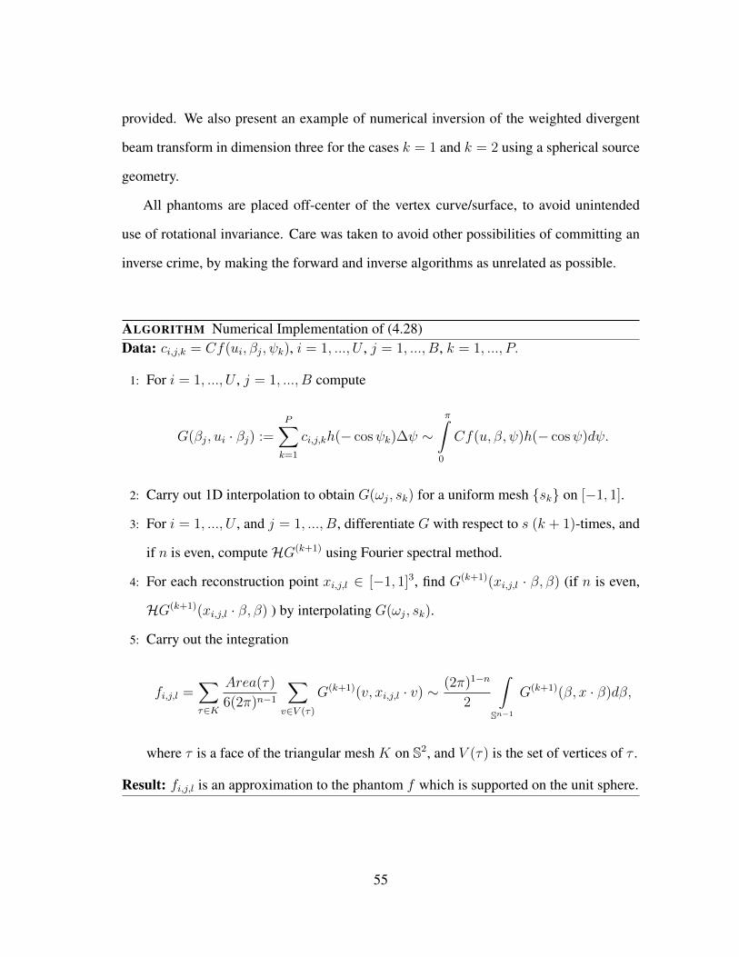
provided. We also present an example of numerical inversion of the weighted divergent
beam transform in dimension three for the cases k = 1 and k = 2 using a spherical source
geometry.
All phantoms are placed off-center of the vertex curve/surface, to avoid unintended
use of rotational invariance. Care was taken to avoid other possibilities of committing an
inverse crime, by making the forward and inverse algorithms as unrelated as possible.
ALGORITHM Numerical Implementation of (4.28)Data: ci,j,k = Cf(ui, βj, ψk), i = 1, ..., U , j = 1, ..., B, k = 1, ..., P.
1: For i = 1, ..., U , j = 1, ..., B compute
G(βj, ui · βj) :=P∑k=1
ci,j,kh(− cosψk)∆ψ ∼π∫
0
Cf(u, β, ψ)h(− cosψ)dψ.
2: Carry out 1D interpolation to obtain G(ωj, sk) for a uniform mesh {sk} on [−1, 1].
3: For i = 1, ..., U , and j = 1, ..., B, differentiate G with respect to s (k + 1)-times, and
if n is even, computeHG(k+1) using Fourier spectral method.
4: For each reconstruction point xi,j,l ∈ [−1, 1]3, find G(k+1)(xi,j,l · β, β) (if n is even,
HG(k+1)(xi,j,l · β, β) ) by interpolating G(ωj, sk).
5: Carry out the integration
fi,j,l =∑τ∈K
Area(τ)
6(2π)n−1
∑v∈V (τ)
G(k+1)(v, xi,j,l · v) ∼ (2π)1−n
2
∫Sn−1
G(k+1)(β, x · β)dβ,
where τ is a face of the triangular mesh K on S2, and V (τ) is the set of vertices of τ .
Result: fi,j,l is an approximation to the phantom f which is supported on the unit sphere.
55
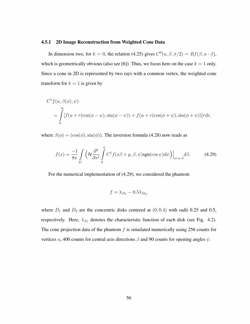
4.5.1 2D Image Reconstruction from Weighted Cone Data
In dimension two, for k = 0, the relation (4.25) gives C0(u, β, π/2) = Rf(β, u · β),
which is geometrically obvious (also see [6]). Thus, we focus here on the case k = 1 only.
Since a cone in 2D is represented by two rays with a common vertex, the weighted cone
transform for k = 1 is given by
C1f(u, β(φ), ψ)
=
∞∫0
[f(u+ r(cos(φ− ψ), sin(φ− ψ)) + f(u+ r(cos(φ+ ψ), sin(φ+ ψ))]rdr,
where β(φ) = (cos(φ), sin(φ)). The inversion formula (4.28) now reads as
f(x) =−1
8π
∫S1
(H ∂2
∂s2
π∫0
C1f(sβ + y, β, ψ)sgn(cosψ)dψ)∣∣∣
s=x·βdβ. (4.29)
For the numerical implementation of (4.29), we considered the phantom
f = χD1 − 0.5χD2 ,
where D1 and D2 are the concentric disks centered at (0, 0.4) with radii 0.25 and 0.5,
respectively. Here, χDi denotes the characteristic function of each disk (see Fig. 4.2).
The cone projection data of the phantom f is simulated numerically using 256 counts for
vertices u, 400 counts for central axis directions β and 90 counts for opening angles ψ.
56

Figure 4.2: The density plot (left) and surface plot (right) of the phantom f that consists oftwo concentric disks centered at (0, 0.4) with radii 0.25 and 0.5, and densities 1 and -0.5units, respectively.
Figure 4.3: The density plot of 256 × 256 image reconstructed from the simulated conedata using 256 counts for vertices u (represented by white dots on the unit circle), 400counts for directions β and 90 counts for opening angles ψ (left), and the comparison ofy-axis profiles of the phantom and the reconstruction (right).
57

Figure 4.4: The density plot of 256×256 image reconstructed from cone data contaminatedwith 5% Gaussian noise (left), and the comparison of y-axis profiles of the phantom andthe reconstruction (right). The dimensions of the cone data are taken as in Fig. 4.3.
As our inversion formula is valid for arbitrary geometry of vertices, we considered
both a circular and a square geometry of vertices of the cones.
Figure 4.3 shows the results of reconstruction from cone projections where the vertices
cover the unit circle. The density plot and the y-axis profile of the reconstruction are
provided in (a) and (b), respectively. The results with a 5% Gaussian white noise added to
the cone data is shown in Figure 4.4.
In Figure 4.5, we provide the results of reconstruction from cone projections where
the vertices are placed along the sides of a square with sides of length two. The density
plot and the y-axis profile of the reconstruction are provided in Figure 4.5 (a) and (b),
respectively. Figure 4.6 shows the results with a 5% Gaussian white noise added to the
cone data.
58
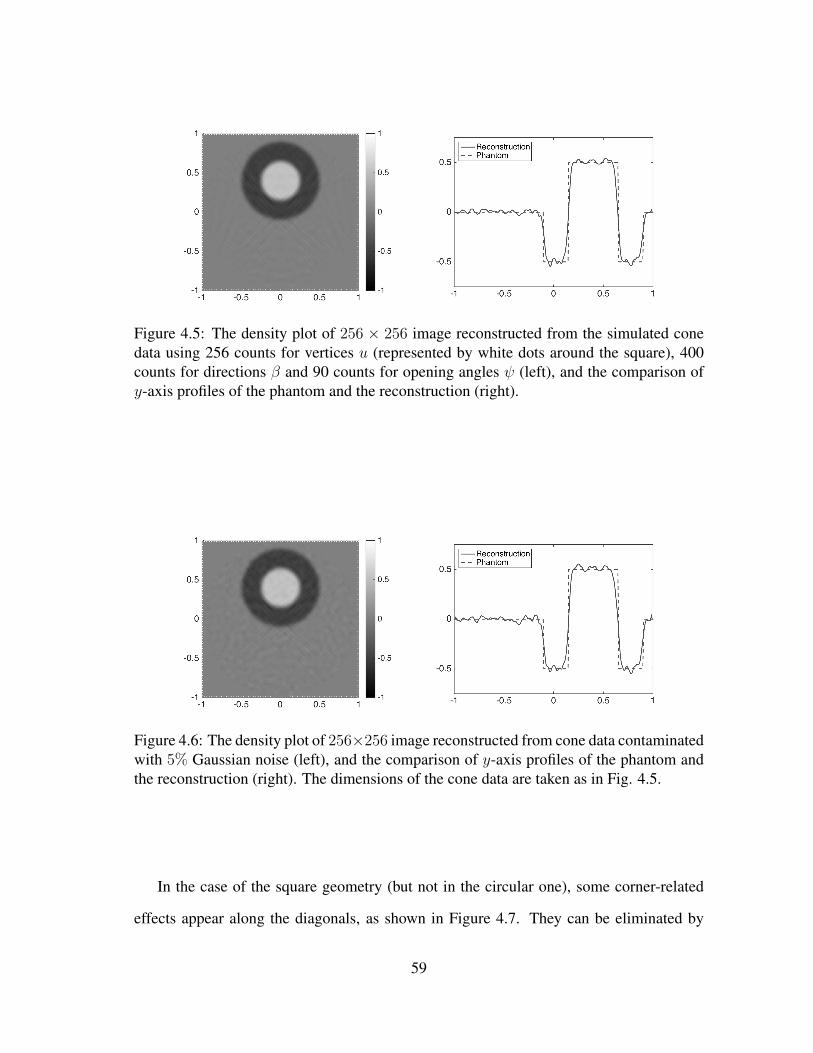
Figure 4.5: The density plot of 256 × 256 image reconstructed from the simulated conedata using 256 counts for vertices u (represented by white dots around the square), 400counts for directions β and 90 counts for opening angles ψ (left), and the comparison ofy-axis profiles of the phantom and the reconstruction (right).
Figure 4.6: The density plot of 256×256 image reconstructed from cone data contaminatedwith 5% Gaussian noise (left), and the comparison of y-axis profiles of the phantom andthe reconstruction (right). The dimensions of the cone data are taken as in Fig. 4.5.
In the case of the square geometry (but not in the circular one), some corner-related
effects appear along the diagonals, as shown in Figure 4.7. They can be eliminated by
59

using a finer discretization in β.
Figure 4.7: Comparison of the profiles of the reconstruction along the diagonal of thesquare region for the circular (left) and square (right) locations of the vertices (detectors).
4.5.2 3D Image Reconstruction from Weighted Cone Data
In dimension three, the relation (4.25) is geometrically obvious for the case k=1 (see
remark 4.2), and is numerically implemented in [6] using spherical harmonic expansions.
Here, we provide examples of reconstruction from the weighted cone data for k = 0 and
k = 2. Theorem 4.4.4 gives the following inversion formula for k = 0:
f(x) =1
8π2
∫S2
( ∂∂s
π∫0
C0f(sβ + y, β, ψ)δ′(cosψ)dψ)∣∣∣
s=x·βdβ
=−1
8π2
∫S2
( ∂∂s
( ∂∂tC0f(sβ + y, β, t)
)∣∣∣t=0
)∣∣∣s=x·β
dβ, (4.30)
and for k = 2, we have
f(x) =−1
16π2
∫S2
( ∂3∂s3
π∫0
C2f(sβ + y, β, ψ)sgn(cosψ)dψ)∣∣∣
s=x·βdβ. (4.31)
60
In our examples, the vertices of the cones cover the unit sphere S2 in R3 and the phan-
tom is the characteristic function of the 3D ball of radius 0.5 units located strictly inside
and off-center of this sphere.
The forward simulations of weighted cone projections were done numerically using
1800 counts for vertices u on the unit sphere, 1800 counts for unit vectors for the cone axis
directions β and 200 counts for opening angles ψ. For the discretization of the sphere, we
used a uniform mesh for both the azimuthal and the polar angles.
Figure 4.8 shows the three cross sections of the spherical phantom and of its recon-
structions from the cone data obtained via (4.30). The comparison of the phantom and the
reconstruction given in Figure 4.8 in terms of their coordinate axis profiles is provided in
Figure 4.9.
Figure 4.8: The 3D ball phantom with radius 0.5, center (0,0,0.25) and unit density (left),and 90×90 image reconstructed via (4.30) from weighted cone data simulated using 1800counts for vertices u on the unit sphere, 1800 counts for directions β and 200 counts foropening angles ψ (right). The cross sections by the planes x = 0, y = 0 and z = 0.25 areshown.
61
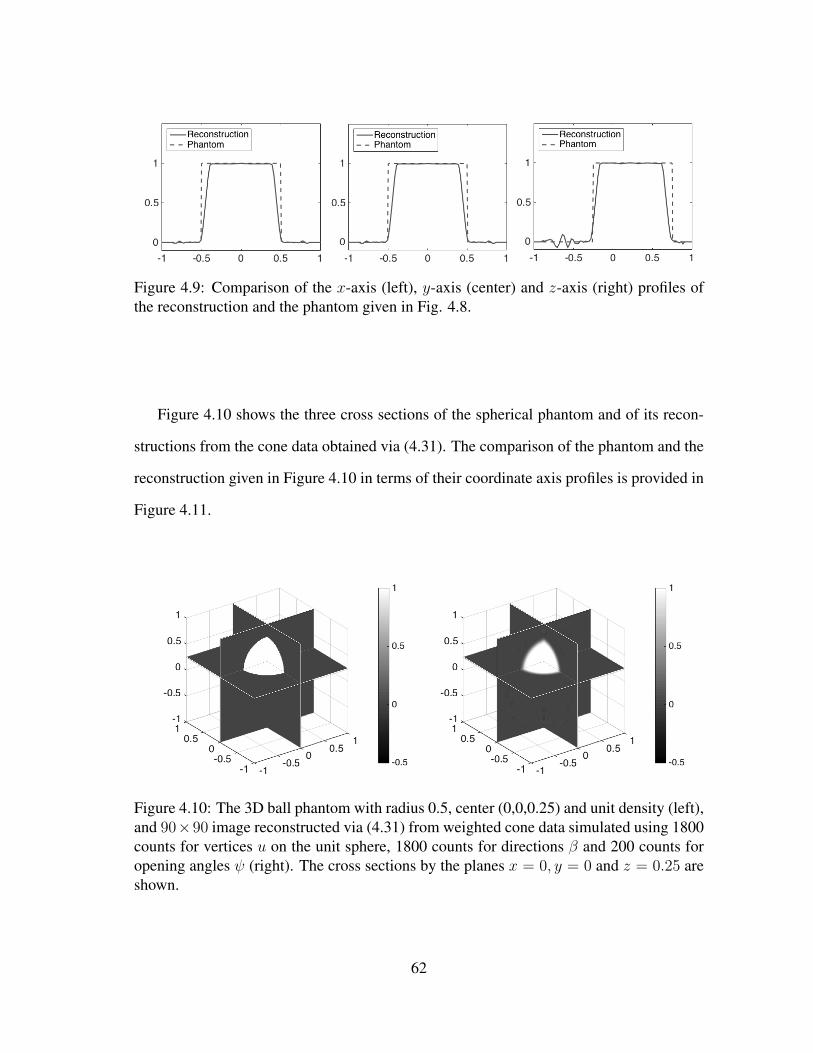
Figure 4.9: Comparison of the x-axis (left), y-axis (center) and z-axis (right) profiles ofthe reconstruction and the phantom given in Fig. 4.8.
Figure 4.10 shows the three cross sections of the spherical phantom and of its recon-
structions from the cone data obtained via (4.31). The comparison of the phantom and the
reconstruction given in Figure 4.10 in terms of their coordinate axis profiles is provided in
Figure 4.11.
Figure 4.10: The 3D ball phantom with radius 0.5, center (0,0,0.25) and unit density (left),and 90×90 image reconstructed via (4.31) from weighted cone data simulated using 1800counts for vertices u on the unit sphere, 1800 counts for directions β and 200 counts foropening angles ψ (right). The cross sections by the planes x = 0, y = 0 and z = 0.25 areshown.
62

Figure 4.11: Comparison of the x-axis (left), y-axis (center) and z-axis (right) profiles ofthe reconstruction and the phantom given in Fig. 4.10.
Figures 4.12 and 4.13 show the results of reconstruction from weighted cone data for
k = 2 contaminated with 5% Gaussian white noise.
Figure 4.12: The 3D ball phantom with radius 0.5, center (0,0,0.25) and unit density (left),and 90 × 90 image reconstructed via (4.31) from weighted cone data contaminated with5% Gaussian white noise (right). The dimensions of the cone projections are taken as inFig. 4.10. The cross sections by the planes x = 0, y = 0 and z = 0.25 are shown.
63
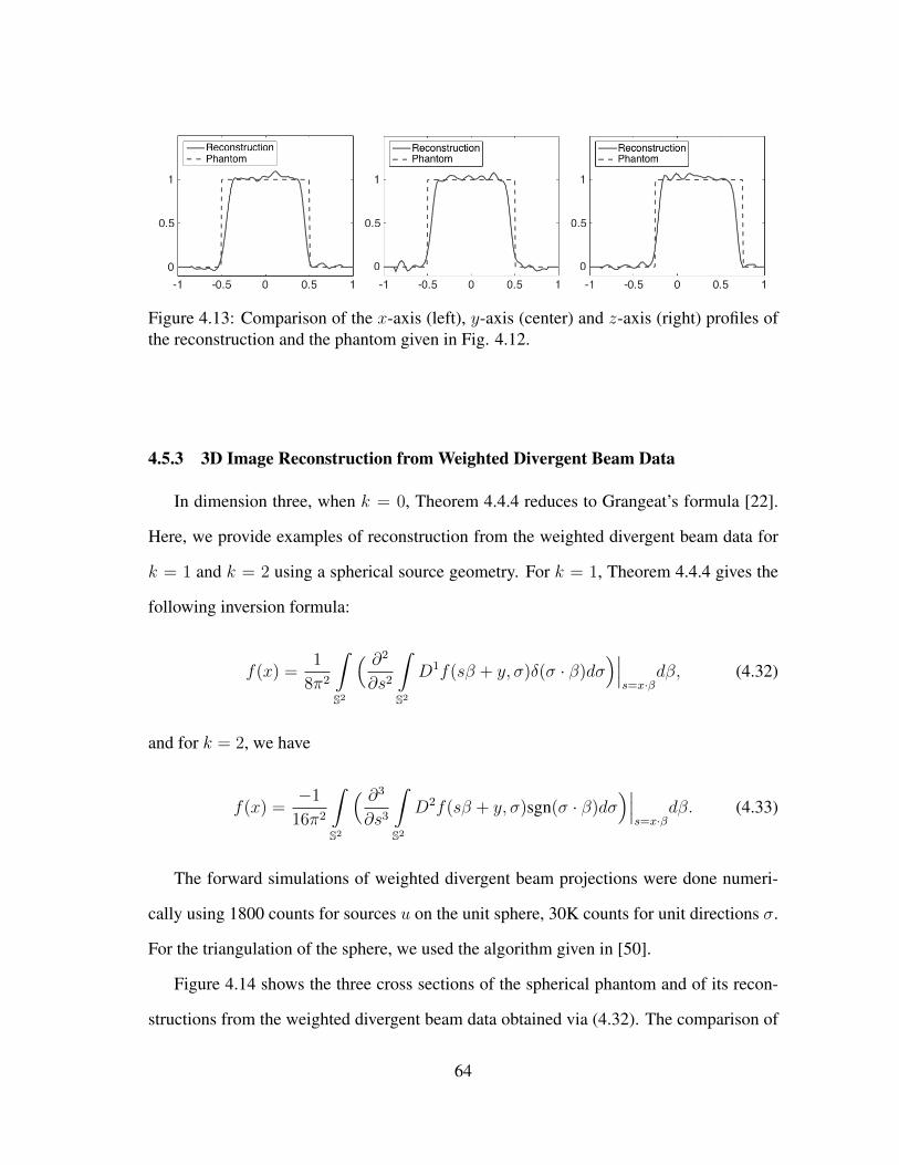
Figure 4.13: Comparison of the x-axis (left), y-axis (center) and z-axis (right) profiles ofthe reconstruction and the phantom given in Fig. 4.12.
4.5.3 3D Image Reconstruction from Weighted Divergent Beam Data
In dimension three, when k = 0, Theorem 4.4.4 reduces to Grangeat’s formula [22].
Here, we provide examples of reconstruction from the weighted divergent beam data for
k = 1 and k = 2 using a spherical source geometry. For k = 1, Theorem 4.4.4 gives the
following inversion formula:
f(x) =1
8π2
∫S2
( ∂2∂s2
∫S2
D1f(sβ + y, σ)δ(σ · β)dσ)∣∣∣
s=x·βdβ, (4.32)
and for k = 2, we have
f(x) =−1
16π2
∫S2
( ∂3∂s3
∫S2
D2f(sβ + y, σ)sgn(σ · β)dσ)∣∣∣
s=x·βdβ. (4.33)
The forward simulations of weighted divergent beam projections were done numeri-
cally using 1800 counts for sources u on the unit sphere, 30K counts for unit directions σ.
For the triangulation of the sphere, we used the algorithm given in [50].
Figure 4.14 shows the three cross sections of the spherical phantom and of its recon-
structions from the weighted divergent beam data obtained via (4.32). The comparison of
64
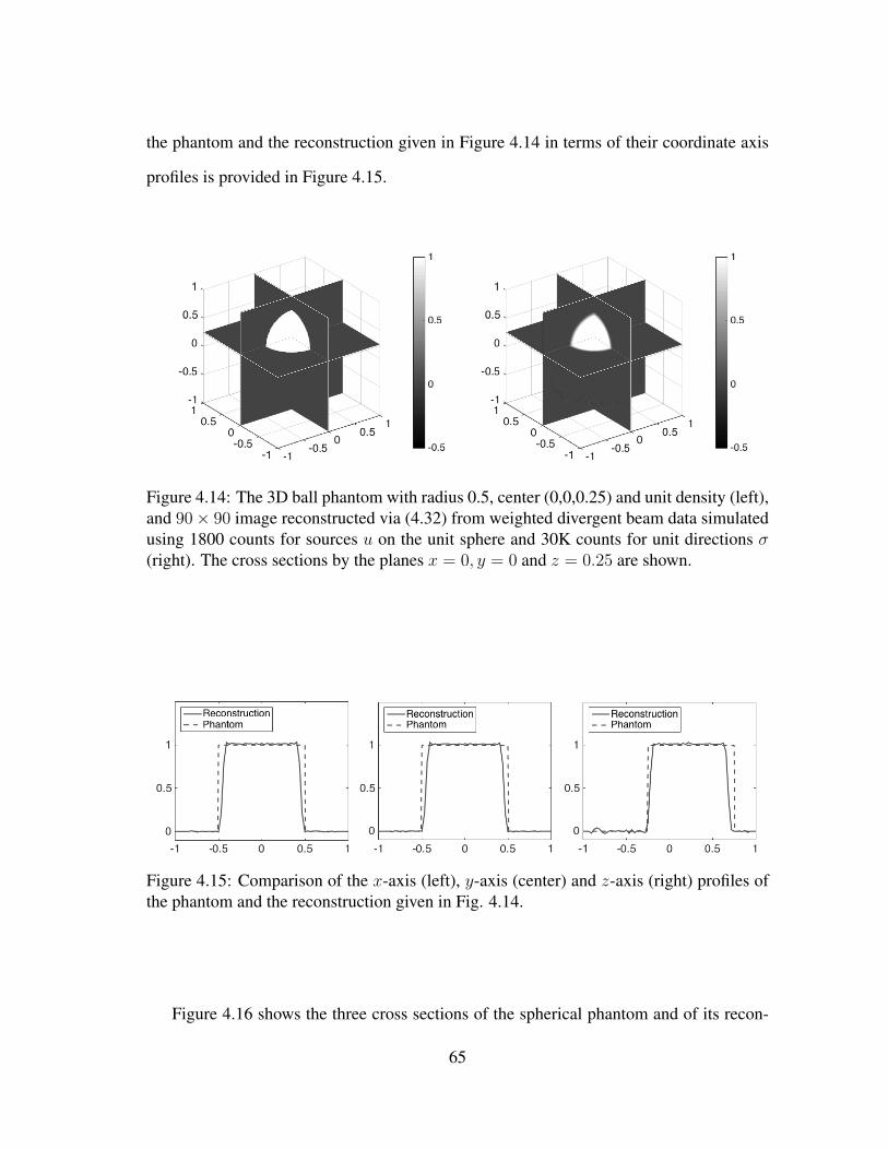
the phantom and the reconstruction given in Figure 4.14 in terms of their coordinate axis
profiles is provided in Figure 4.15.
Figure 4.14: The 3D ball phantom with radius 0.5, center (0,0,0.25) and unit density (left),and 90× 90 image reconstructed via (4.32) from weighted divergent beam data simulatedusing 1800 counts for sources u on the unit sphere and 30K counts for unit directions σ(right). The cross sections by the planes x = 0, y = 0 and z = 0.25 are shown.
Figure 4.15: Comparison of the x-axis (left), y-axis (center) and z-axis (right) profiles ofthe phantom and the reconstruction given in Fig. 4.14.
Figure 4.16 shows the three cross sections of the spherical phantom and of its recon-
65

structions from the weighted divergent beam data obtained via (4.33). The comparison of
the phantom and the reconstruction given in Figure 4.16 in terms of their coordinate axis
profiles is provided in Figure 4.17.
Figure 4.16: The 3D ball phantom with radius 0.5, center (0,0,0.25) and unit density (left),and 90× 90 image reconstructed via (4.33) from weighted divergent beam data simulatedusing 1800 counts for sources u on the unit sphere and 30K counts for unit directions σ(right). The cross sections by the planes x = 0, y = 0 and z = 0.25 are shown.
Figure 4.17: Comparison of the x-axis (left), y-axis (center) and z-axis (right) profiles ofthe reconstruction and the phantom given in Fig. 4.16.
66
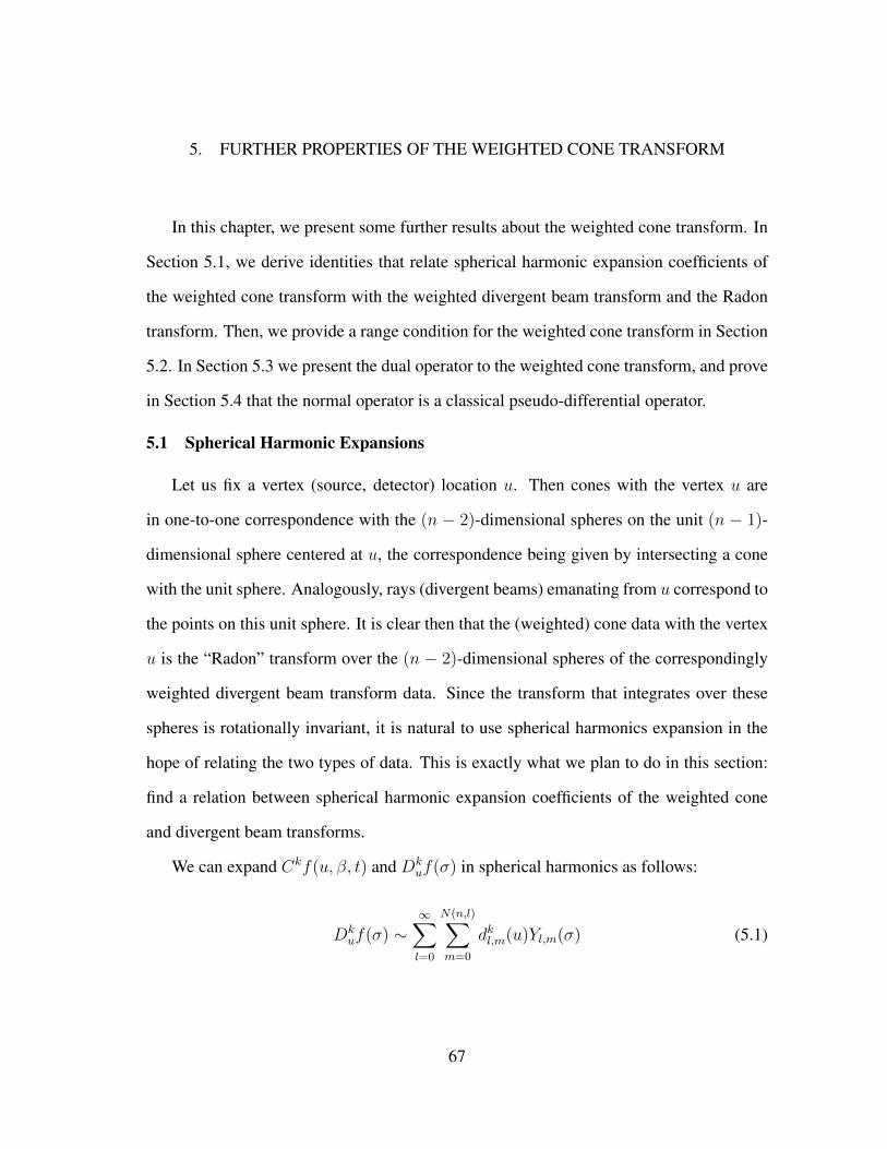
5. FURTHER PROPERTIES OF THE WEIGHTED CONE TRANSFORM
In this chapter, we present some further results about the weighted cone transform. In
Section 5.1, we derive identities that relate spherical harmonic expansion coefficients of
the weighted cone transform with the weighted divergent beam transform and the Radon
transform. Then, we provide a range condition for the weighted cone transform in Section
5.2. In Section 5.3 we present the dual operator to the weighted cone transform, and prove
in Section 5.4 that the normal operator is a classical pseudo-differential operator.
5.1 Spherical Harmonic Expansions
Let us fix a vertex (source, detector) location u. Then cones with the vertex u are
in one-to-one correspondence with the (n − 2)-dimensional spheres on the unit (n − 1)-
dimensional sphere centered at u, the correspondence being given by intersecting a cone
with the unit sphere. Analogously, rays (divergent beams) emanating from u correspond to
the points on this unit sphere. It is clear then that the (weighted) cone data with the vertex
u is the “Radon” transform over the (n − 2)-dimensional spheres of the correspondingly
weighted divergent beam transform data. Since the transform that integrates over these
spheres is rotationally invariant, it is natural to use spherical harmonics expansion in the
hope of relating the two types of data. This is exactly what we plan to do in this section:
find a relation between spherical harmonic expansion coefficients of the weighted cone
and divergent beam transforms.
We can expand Ckf(u, β, t) and Dkuf(σ) in spherical harmonics as follows:
Dkuf(σ) ∼
∞∑l=0
N(n,l)∑m=0
dkl,m(u)Yl,m(σ) (5.1)
67

and
Ckf(u, β, t) ∼∞∑l=0
N(n,l)∑m=0
ckl,m(u, t)Yl,m(β), (5.2)
where Yl,m is the spherical harmonic of degree l and order m (see Appendix B.1.3),
N(n, l) = (n+ 2l − 2)(n+ l − 3)!
l!(n− 2)!, (5.3)
dkl,m(u) =
∫Sn−1
Dkuf(σ)Yl,m(σ)dσ, (5.4)
and
ckl,m(u, t) =
∫Sn−1
Ckf(u, β, t)Yl,m(β)dβ. (5.5)
The following theorem gives a relation between spherical harmonic expansion coefficients
(5.4) and (5.5) of the weighted divergent beam and cone transforms, respectively. This
relation for k = 1 in dimension three was provided in [6].
Theorem 5.1.1. Let P λl (t) be the Gegenbauer (ultraspherical) polynomials of degree l,
λ > −1/2 (see Appendix B.1.2). Then, for any u ∈ Rn,
ckl,m(u, t) =
|Sn−2|(1− t2)(n−2)/2P (n−2)/2
l (t)dkl,m(u), |t| ≤ 1
0, |t| > 1.
(5.6)
Proof. In view of (4.4), it is clear that ckl,m(u, t) = 0 when |t| > 1. For |t| ≤ 1, we can
68
write
ckl,m(u, t) =
∫Sn−1
Ckf(u, β, t)Yl,m(β)dβ
=√
1− t2∫
Sn−1
∫Sn−1
Dkuf(σ)δ(σ · β − t)dσ Yl,m(β)dβ
=√
1− t2∫
Sn−1
Dkuf(σ)
∫Sn−1
δ(σ · β − t)Yl,m(β)dβ dσ.
Here, we can apply Funk-Hecke formula (see Theorem B.1.1) to obtain
∫Sn−1
δ(σ · β − t)Yl,m(β)dβ = |Sn−2|(1− t2)(n−3)/2P (n−2)/2l (t)Yl,m(σ).
Hence,
ckl,m(u, t) = |Sn−2|(1− t2)(n−2)/2P (n−2)/2l (t)
∫Sn−1
Dkuf(σ)Yl,m(σ)dσ,
which implies (5.6).
When k = n − 2, we can use the relation of the cosine transform with spherical
harmonics to find a relation between the spherical harmonic expansion coefficients of the
cone and Radon transforms.
Lemma 5.1.2. Let g ∈ L1(Sn−1). Then,
∫Sn−1
π∫0
Cf(u, β, ψ)g(β) sinψdψdβ = π
∫Sn−1
Rf(ω, ω · u)Cg(ω)dω. (5.7)
Proof. Multiplying both sides of (3.10) with g(β) and integrating with respect to β over
69
Sn−1, we have
∫Sn−1
π∫0
Cf(u, β, ψ)g(β) sinψdψdβ =π
|Sn−1|
∫Sn−1
Rf(ω, ω · u)
∫Sn−1
g(β)|ω · β|dβdω
= π
∫Sn−1
Rf(ω, ω · u)Cg(ω)dω.
The spherical harmonics are known to be the eigenfunctions of the cosine transform.
This follows from the Funk-Hecke Formula (B.1.1).
Corollary 5.1.3. For every spherical harmonic Yl of degree l, l = 0, 1, 2, ..., and every
ω ∈ Sn−1,
CYl(ω) = λlYl(ω) (5.8)
where λl is given as in Funk-Hecke Formula (Theorem B.1.1) for f(t) = |t|.
Now, we can establish the following relation.
Proposition 5.1.4. For every spherical harmonic Yl of degree l,
∫Sn−1
π∫0
Cf(u, β, ψ)Yl(β) sinψdψdβ = πλl
∫Sn−1
Rf(ω, ω · u)Yl(ω)dω. (5.9)
In particular, for l = 0, we obtain (3.15).
Proof. Letting g = Yl in (5.7), and using (5.8), we get (5.9). Then, the equation (3.15)
follows from direct calculation.
Remark 5.1.5. As the relation (5.9) gives the spherical harmonics coefficients of the func-
tion Rf(ω, u · ω), one can recover it for all u ∈ Rn and ω ∈ Sn−1. Then, any inversion
70

formula for the Radon transform (B.16) would reconstruct the function f . This can be
considered as an analog of Cormack’s method [46].
5.2 A Range Condition
Theorem 5.2.1. Suppose that f ∈ S(Rn). For any k ∈ Z+ and u ∈ Rn, the weighted
cone transform Ckuf(β, t) satisfies the following differential equation.
{a2(n, t)
∂2
∂t2+ a1(n, t)
∂
∂t+ a0(n, t) + b(n, t)∆S
}g(β, t) = 0 on Sn−1 × (−1, 1)
g(β,−1) = g(β, 1) = 0, (5.10)
where
a0(n, t) =1
2(n− 2)[(n− 1)t− n],
a1(n, t) = −1
2(2t+ n− 2)(1− t2), (5.11)
a2(n, t) = (1− t2)2,
b(n, t) = −(1− t2).
Proof. Let λ = (n − 2)/2. It is well known that P λl (t) solves the following differential
equation (see Appendix B.1.2):
(1− t2)y′′ − (n− 1)ty′ + l(l + 2λ)y = 0. (5.12)
71

Let y(t) = P λl (t), and y(t) = (1− t2)λy(t). Then, for t ∈ (−1, 1),
y(t) = (1− t2)−λy(t),
y′(t) = (1− t2)−λ−1[(1− t2)y′(t)− λy(t)
], (5.13)
y′′(t) = (1− t2)−λ−2[(1− t2)2y′′(t)− λ(2t− 1)(1− t2)y′(t)− 2λ(λ+ 1)ty(t)
].
Plugging (5.13) in (B.6), we obtain
(1− t2)2y′′ − (t+ λ)(1− t2)y′
+[λ(2λ+ 1)t− 2λ(λ+ 1) + l(l + 2λ)(1− t2)
]y = 0.
Then, (5.6) implies that for any k ∈ Z+ and u ∈ Rn, ckl,m(u, t) satisfies
{a2(n, t)
∂2
∂t2+ a1(n, t)
∂
∂t+ a0(n, t) + b(n, t)(−l)(l + n− 2)
}ckl,m(u, t) = 0, (5.14)
where ai(n, t), i = 0, 1, 2, and b(n, t) is as in (5.11). Now, since
∆SYl,m = −l(l + n− 2)Yl,m l = 0, 1, 2, ... (5.15)
we obtain
{a2(n, t)
∂2
∂t2+ a1(n, t)
∂
∂t+ a0(n, t) + b(n, t)∆S
}ckl,m(u, t)Yl,m(β) = 0, (5.16)
whose application in (5.2) implies the theorem.
72
5.3 Dual Operator
Let Z = Rn × Sn−1 × (−1, 1), w ∈ C∞c (Rn) be a weight function, and
L2w(Z) :=
g : Z → R | ||g||L2w(Z)
=
∫Z
|g(u, β, t)|2 w(u)
1− t2dtdβdu
1/2
<∞
.
Theorem 5.3.1. Let Ck# be the operator defined on L2
w(Z) as
Ck#g(x) =
∫Z
g(x− y, β, t)δ(y · β − |y|t) |y|k−n+2w(x− y)√
1− t2dtdβdy
=
∫Rn
∫Sn−1
g(x− y, β, y|y|· β)|y|k−n+1w(x− y)√
1−(y|y| · β
)2 dβdy. (5.17)
Then, Ck, Ck# form a dual pair, that is for f ∈ S(Rn), we have
(Ckf, g)L2w(Z)
= (f, Ck#g)L2(Rn)
73

Proof. By definition of the cone transform (4.3),
(Ckf, g)L2w(Z)
=
∫Z
Ckf(u, β, t)g(u, β, t)w(u)
1− t2dtdβdu
=
∫Z
∫Rn
f(x)δ((x− u) · β − |x− u|t)|x− u|k−n+2dx g(u, β, t)w(u)√1− t2
dtdβdu
=
∫Rn
f(x)
∫Z
g(u, β, t)δ((x− u) · β − |x− u|t) |x− u|k−n+2w(u)√1− t2
dtdβdu
dx
=
∫Rn
f(x)
∫Z
g(x− y, β, t)δ(y · β − |y|t) |y|k−n+2w(x− y)√
1− t2dtdβdy
dx
=
∫Rn
f(x)Ck#g(x)dx = (f, Ck
#g)L2(Rn).
5.4 A Microlocal Property
It is rather standard in tomography to consider the normal operator Ck#C
k, and study
its properties.
Theorem 5.4.1. The normal operator Ck#C
k is a classical pseudo-differential operator
(see e.g., [23, 55]) of order 1− n,
Ck#C
kf(x) =
∫Rn
∫Rn
ei(x−y)·ξa(x, y, ξ)f(y)dydξ,
with an amplitude
a(x, y, ξ) = a0(x, y)|ξ|1−n,
74
where
a0(x, y) = 2
∫Rn
|x− y||(x− u)(2u− v)|k−n+2w(u)
||x− u|(y − u)− |y − u|(x− u)|du.
Proof. We compute the normal operator
Ck#C
kf(x) =
∫Rn
∫Sn−1
Ckf(x− y, β, y|y|· β)|y|k−n+2w(x− y)√
1−(y|y| · β
)2 dβ dy|y|=
∫Rn
∫Sn−1
∫Rn
f(x− y + z)δ(z · β − |z| y|y|· β)|x− y − z|k−n+2dz |y|k−n+2w(x− y)dβ
dy
|y|
=
∫Rn
∫Sn−1
∫Rn
f(x+ z − y)δ((|y|z − |z|y) · β)w(x− y)|y(x− y − z)|k−n+2dydβdz,
where we have used δ(a(x− y)) =1
aδ(x− y).
Now, for fixed y, z ∈ Rn, y 6= z,
|y|z − |z|y =||y|z − |z|y||z − y|
A(z − y)
for some the rotation matrix A depending on y and z. Thus,
δ((|y|z − |z|y) · β) = δ(||y|z − |z|y||z − y|
A(z − y) · β) =|z − y|
||y|z − |z|y|δ((z − y) · A−1β).
As the Lebesgue measure on Sn−1 is rotation invariant, we obtain
Ck#C
kf(x) =∫Rn
∫Sn−1
∫Rn
f(x+ z − y)|z − y|
||y|z − |z|y|δ((z − y) · β)w(x− y)|y(x− y − z)|k−n+2dydβdz.
75

As δ((z − y) · β) =
∞∫−∞
e−i[(z−y)·β]rdr, we have
∫Sn−1
δ((z − y) · β)dβ =
∫Sn−1
∞∫−∞
e−i[(z−y)·β]rdrdβ
Letting ξ = rβ and using rotation invariance of Lebesgue measure, we obtain
∫Sn−1
∞∫−∞
e−i[(z−y)·β]rdrdβ = 2
∫Rn
e−i(z−y)·ξ|ξ|1−ndξ.
Therefore,
Ck#C
kf(x)
= 2
∫Rn
∫Rn
∫Rn
e−i(z−y)·ξf(x+ z − y)w(x− y)|z − y||y(x− y − z)|k−n+2
||y|z − |z|y|dydz|ξ|1−ndξ
= 2
∫Rn
∫Rn
∫Rn
ei(x−v)·ξf(v)|x− v||y(2(x− y)− v))|k−n+2w(x− y)
||y|(v − x+ y)− |v − x+ y|y|dydv|ξ|1−ndξ
= 2
∫Rn
∫Rn
∫Rn
ei(x−v)·ξf(v)|x− v||(x− u)(2u− v)|k−n+2w(u)
||x− u|(v − u)− |v − u|(x− u)|dudv|ξ|1−ndξ,
where we changed variables in z by letting v = x + z − y, and then in y by u = x − y.
Hence,
Ck#C
kf(x) =
∫Rn
∫Rn
ei(x−v)·ξa0(x, v)|ξ|1−nf(v)dvdξ,
where
a0(x, v) = 2
∫Rn
|x− v||(x− u)(2u− v)|k−n+2w(u)
||x− u|(v − u)− |v − u|(x− u)|du.
76

Finally letting
a(x, v, ξ) = a0(x, v)|ξ|1−n
implies the result.
77
6. CONCLUSION AND REMARKS
In this dissertation, the (weighted) cone transform was investigated in terms of its
invertibility, range conditions and microlocal properties. It was argued that in the case
of Compton camera imaging, reducing the set of cones “visible” from a detector (e.g.,
considering only the cones with a given axial direction), which was done in most previous
studies, seems not to be a very good idea (especially in presence of low signal-to-noise
ratio), since this amounts to discarding the already collected data while it could be used for
stabilizing the reconstruction. We thus considered the full data (weighted) cone transform,
and derived various inversion formulas that are applicable for a wide variety of detector
geometries in any dimension. We note that it is common to have a variety of different
inversion formulas for Radon type transforms, which are all the same for perfect data,
but react differently to unavoidable errors in data. Having such a variety is even more
important when dealing with overdetermined data, as in Compton camera imaging.
A closely related to the weighted cone transform is what is called weighted divergent
beam transform. When the weight factor is not present, this is the well studied and im-
portant for the 3D X-ray CT divergent (or cone) beam transform. We thus studied it in
some details, derived various inversion formulas and implemented them numerically in
dimension three.
One of the most important features, in the author’s view, is that the new formulas are
adjustable to a wide variety of (detector) geometries. We introduced the class of such
geometries satisfying what we call in Chapter 4 the Tuy’s condition (its weaker form was
defined as Compton admissibility condition in Chapter 3). Most of the previously derived
formulas required very symmetric geometries, allowing for harmonic analysis tools to be
used. This is also related to the important issue of understanding the geometries that allow
78
for (stable) reconstruction. They deserve a much more thorough study, which we plan to
address in future work.
As it was mentioned in the introduction, to avoid being distracted from the main pur-
pose of this text, we assumed that the functions to be reconstructed belong to the Schwartz
space S. However, as in the case of Radon transform (see, e.g. [36, 46]), the results un-
doubtedly have a much wider area of applicability, since the derived formulas can be ex-
tended by continuity to some wider function spaces. Although we haven’t done this in the
current text, this conclusion is confirmed, in particular, by our successful numerical imple-
mentations for discontinuous (piecewise continuous) phantoms. The issues of appropriate
function spaces will be addressed elsewhere.
Practical soundness of the derived inversion techniques is shown by their numerical
implementation in the most interesting dimensions two and three. The implementation of
the 3D inversion algorithms in Chapter 3 is challenging due to the high dimensionality of
the forward data, and the fact that the application of a fourth order differential operator on
the unit sphere to a singular integral is required. We thus develop and apply three different
inversion algorithms and study their feasibility. One should also notice, that the algorithm
of the 3D cone transform inversion in Chapter 4 works much faster than some of the ones
developed in Chapter 3. The reason is that a much coarser mesh (1.8K nodes) on the
sphere suffices, rather than 30K used in Chapter 3.
79
REFERENCES
[1] M. ALLMARAS, D. DARROW, Y. HRISTOVA, G. KANSCHAT, AND P. KUCHMENT,
Detecting small low emission radiating sources, Inverse Problems and Imaging, 7
(2013), pp. 47–79.
[2] G. AMBARTSOUMIAN, Inversion of the V-line Radon transform in a disc and its
applications in imaging, Computers & Mathematics with Applications, 64 (2012),
pp. 260–265.
[3] G. AMBARTSOUMIAN AND S. MOON, A series formula for inversion of the V-line
Radon transform in a disc, Computers & Mathematics with Applications, 66 (2013),
pp. 1567–1572.
[4] G. AMBARTSOUMIAN AND S. ROY, Numerical inversion of a broken ray transform
arising in single scattering optical tomography, IEEE Transactions on Computa-
tional Imaging, 2 (2016), pp. 166–173.
[5] S. R. ARRIDGE, Optical tomography in medical imaging, Inverse problems, 15
(1999), p. R41.
[6] R. BASKO, G. L. ZENG, AND G. T. GULLBERG, Application of spherical har-
monics to image reconstruction for the Compton camera, Physics in Medicine and
Biology, 43 (1998), p. 887.
[7] M. BELKIN, J. SUN, AND Y. WANG, Discrete Laplace operator on meshed surfaces,
in Proceedings of the twenty-fourth annual symposium on computational geometry,
ACM, 2008, pp. 278–287.
[8] M. J. CREE AND P. J. BONES, Towards direct reconstruction from a gamma camera
based on Compton scattering, IEEE transactions on medical imaging, 13 (1994),
80

pp. 398–407.
[9] D. B. EVERETT, J. S. FLEMING, R. W. TODD, AND J. M. NIGHTINGALE, Gamma-
radiation imaging system based on the Compton effect, Electrical Engineers, Pro-
ceedings of the Institution of, 124 (1977), p. 995.
[10] L. FLORESCU, V. A. MARKEL, AND J. C. SCHOTLAND, Single-scattering opti-
cal tomography: Simultaneous reconstruction of scattering and absorption, Physical
Review E, 81 (2010), p. 016602.
[11] , Inversion formulas for the broken-ray Radon transform, Inverse Problems, 27
(2011), p. 025002.
[12] L. FLORESCU, J. C. SCHOTLAND, AND V. A. MARKEL, Single-scattering optical
tomography, Physical Review E, 79 (2009), p. 036607.
[13] P. FUNK, Über flächen mit lauter geschlossenen geodätischen linien, Mathematische
Annalen, 74 (1913), pp. 278–300.
[14] R. J. GARDNER, Geometric Tomography, vol. 6, Cambridge University Press Cam-
bridge, 1995.
[15] I. M. GEL’FAND, S. G. GINDIKIN, AND M. I. GRAEV, Selected Topics in Integral
Geometry, vol. 220, American Mathematical Soc., 2003.
[16] I. M. GEL’FAND AND A. B. GONCHAROV, Recovery of a compactly supported
function starting from its integrals over lines intersecting a given set of points in
space, in Soviet Math. Dokl, vol. 34, 1987, pp. 373–376.
[17] I. M. GEL’FAND AND G. E. SHILOV, Generalized Functions, Volume 1: Properties
and Operations, Academic, New York, 1964.
[18] Y. N. GEORGIEVA-HRISTOVA, Mathematical Problems of Thermoacoustic and
Compton Camera Imaging, PhD thesis, Texas A&M University, 2010.
81
[19] P. GOODEY AND W. WEIL, Centrally symmetric convex bodies and the spherical
Radon transform, Journal of Differential Geometry, 35 (1992), pp. 675–688.
[20] R. GOUIA-ZARRAD, Analytical reconstruction formula for n-dimensional coni-
cal Radon transform, Computers & Mathematics with Applications, 68 (2014),
pp. 1016–1023.
[21] R. GOUIA-ZARRAD AND G. AMBARTSOUMIAN, Exact inversion of the conical
Radon transform with a fixed opening angle, Inverse Problems, 30 (2014), p. 045007.
[22] P. GRANGEAT, Mathematical framework of cone beam 3D reconstruction via the
first derivative of the Radon transform, in Mathematical methods in tomography,
Springer, 1991, pp. 66–97.
[23] A. GRIGIS AND J. SJÖSTRAND, Microlocal analysis for differential operators: an
introduction, vol. 196, Cambridge University Press, 1994.
[24] M. HALTMEIER, Exact reconstruction formulas for a Radon transform over cones,
Inverse Problems, 30 (2014), p. 035001.
[25] C. HAMAKER, K. T. SMITH, D. C. SOLMON, AND S. L. WAGNER, The divergent
beam x-ray transform, Rocky Mt. J. Math., 10 (1980).
[26] S. HELGASON, Integral Geometry and Radon Transforms, Springer Science & Busi-
ness Media, 2010.
[27] Y. HRISTOVA, Inversion of a V-line transform arising in emission tomography, Jour-
nal of Coupled Systems and Multiscale Dynamics, 3 (2015), pp. 272–277.
[28] M. HUBENTHAL, The broken ray transform on the square, Journal of Fourier Anal-
ysis and Applications, 20 (2014), pp. 1050–1082.
[29] J. ILMAVIRTA, Broken ray tomography in the disc, Inverse Problems, 29 (2013),
p. 035008.
82

[30] C.-Y. JUNG AND S. MOON, Inversion formulas for cone transforms arising in ap-
plication of Compton cameras, Inverse Problems, 31 (2015), p. 015006.
[31] , Exact inversion of the cone transform arising in an application of a Compton
camera consisting of line detectors, SIAM Journal on Imaging Sciences, 9 (2016),
pp. 520–536.
[32] A. KATSEVICH, Theoretically exact filtered backprojection-type inversion algorithm
for spiral ct, SIAM Journal on Applied Mathematics, 62 (2002), pp. 2012–2026.
[33] , An improved exact filtered backprojection algorithm for spiral computed to-
mography, Advances in Applied Mathematics, 32 (2004), pp. 681–697.
[34] A. KATSEVICH AND R. KRYLOV, Broken ray transform: inversion and a range
condition, Inverse Problems, 29 (2013), p. 075008.
[35] R. KRYLOV AND A. KATSEVICH, Inversion of the broken ray transform in the
case of energy-dependent attenuation, Physics in medicine and biology, 60 (2015),
p. 4313.
[36] P. KUCHMENT, The Radon transform and medical imaging, vol. 85, SIAM, 2014.
[37] P. KUCHMENT AND F. TERZIOGLU, Three-dimensional image reconstruction from
Compton camera data, SIAM Journal on Imaging Sciences, 9 (2016), pp. 1708–
1725.
[38] , Inversion of weighted divergent beam and cone transforms, Inverse Problems
& Imaging, 11 (2017), pp. 1071–1090.
[39] A. K. LOUIS AND P. MAASS, A mollifier method for linear operator equations of
the first kind, Inverse problems, 6 (1990), p. 427.
83

[40] A. K. LOUIS, M. RIPLINGER, M. SPIESS, AND E. SPODAREV, Inversion algo-
rithms for the spherical Radon and cosine transform, Inverse Problems, 27 (2011),
p. 035015.
[41] R. B. MARR, C.-N. CHEN, AND P. C. LAUTERBUR, On two approaches to 3d
reconstruction in nmr zeugmatography, in Mathematical aspects of computerized
tomography, Springer, 1981, pp. 225–240.
[42] V. MAXIM, Filtered backprojection reconstruction and redundancy in Compton
camera imaging, IEEE Transactions on Image Processing, 23 (2014), pp. 332–341.
[43] V. MAXIM, M. FRANDES, AND R. PROST, Analytical inversion of the Compton
transform using the full set of available projections, Inverse Problems, 25 (2009),
p. 095001.
[44] M. MORVIDONE, M. K. NGUYEN, T. T. TRUONG, AND H. ZAIDI, On the V-line
Radon transform and its imaging applications, Journal of Biomedical Imaging, 2010
(2010), p. 11.
[45] C. MÜLLER, Spherical harmonics, Springer, 1966.
[46] F. NATTERER, The mathematics of computerized tomography, vol. 32, Siam, 1986.
[47] M. K. NGUYEN, T. T. TRUONG, AND P. GRANGEAT, Radon transforms on a class
of cones with fixed axis direction, Journal of Physics A: Mathematical and General,
38 (2005), p. 8003.
[48] A. OLSON, A. CIABATTI, Y. HRISTOVA, P. KUCHMENT, J. RAGUSA, AND
M. ALLMARAS, Passive detection of small low-emission sources: Two-dimensional
numerical case studies, Nuclear Science and Engineering, 184 (2016), pp. 125–150.
[49] V. PALAMODOV, Reconstructive integral geometry, vol. 98, Springer Science &
Business Media, 2004.
84

[50] P.-O. PERSSON AND G. STRANG, A simple mesh generator in matlab, SIAM re-
view, 46 (2004), pp. 329–345.
[51] M. RIPLINGER AND M. SPIESS, Numerical inversion of the spherical Radon trans-
form and the cosine transform using the approximate inverse with a special class of
locally supported mollifiers, Journal of Inverse and Ill-posed Problems, 22 (2014),
pp. 497–536.
[52] B. RUBIN, Introduction to Radon transforms, vol. 160, Cambridge University Press,
2015.
[53] J. C. SCHOTLAND, Direct reconstruction methods in optical tomography, in Mathe-
matical Modeling in Biomedical Imaging II, Springer, 2012, pp. 1–29.
[54] B. SHERSON, Some Results in Single-Scattering Tomography, PhD thesis, Oregon
State University, 2015.
[55] M. A. SHUBIN AND S. I. ANDERSSON, Pseudodifferential operators and spectral
theory, vol. 200, Springer, 1987.
[56] M. SINGH, An electronically collimated gamma camera for single photon emission
computed tomography. part i: Theoretical considerations and design criteria, Medi-
cal Physics, 10 (1983), pp. 421–427.
[57] B. SMITH, Reconstruction methods and completeness conditions for two Compton
data models, JOSA A, 22 (2005), pp. 445–459.
[58] B. D. SMITH, Image reconstruction from cone-beam projections: necessary and suf-
ficient conditions and reconstruction methods, IEEE transactions on medical imag-
ing, 4 (1985), pp. 14–25.
[59] E. M. STEIN AND G. WEISS, Introduction to Fourier analysis on Euclidean spaces,
vol. 32, Princeton university press, 2016.
85
[60] F. TERZIOGLU, Some inversion formulas for the cone transform, Inverse Problems,
31 (2015), p. 115010.
[61] T. T. TRUONG AND M. K. NGUYEN, On new-line Radon transforms in and their
inversion, Journal of Physics A: Mathematical and Theoretical, 44 (2011), p. 075206.
[62] , New properties of the V-line Radon transform and their imaging applications,
Journal of Physics A: Mathematical and Theoretical, 48 (2015), p. 405204.
[63] H. K. TUY, An inversion formula for cone-beam reconstruction, SIAM Journal on
Applied Mathematics, 43 (1983), pp. 546–552.
[64] F. WUBBELING AND F. NATTERER, Mathematical methods in image reconstruction,
SIAM, Philadelphia, 8 (2001), p. 16.
[65] X. XUN, B. MALLICK, R. J. CARROLL, AND P. KUCHMENT, A Bayesian ap-
proach to the detection of small low emission sources, Inverse problems, 27 (2011),
p. 115009.
86

APPENDIX A
AN ALTERNATIVE PROOF OF THEOREM 3.3.1
Here we prove Theorem 3.3.1 in an alternative way, which avoids reference to the
relation (B.31).
As in the case of the Radon transform, invariance properties play a key role in the inver-
sion of the cone transform. In fact, due to rotational invariance, it suffices to prove (3.10)
only for the vertical cone transform. Moreover, shift invariance enables us to consider
vertical cones having vertex at the origin only, that is u = 0.
Proposition A.0.1. For any f ∈ S(Rn), we have
π∫0
Cf(0, en, ψ) sinψdψ =π
|Sn−1|
∫Sn−1
Rf(ω, 0)|ω · en|dω. (A.1)
We first prove the proposition for n = 2. By definition of the 2-dimensional cone
transform (3.4), we have
π∫0
Cf(0, e2, ψ) sinψdψ =
π∫0
∞∫0
f(r sinψ, r cosψ) sinψdrdψ
+
π∫0
∞∫0
f(−r sinψ, r cosψ) sinψdrdψ.
87
Changing variables by letting r → −r and ψ → π − ψ, respectively, we obtain
π∫0
∞∫0
f(r sinψ, r cosψ) sinψdrdψ =
π∫0
0∫−∞
f(−r sinψ,−r cosψ) sinψdrdψ
=
π∫0
0∫−∞
f(−r sinφ, r cosφ) sinφdrdφ.
Therefore,
π∫0
Cf(0, e2, ψ) sinψdψ =
π∫0
∞∫−∞
f(−r sinψ, r cosψ) sinψdrdψ
=
π∫0
Rf(ω(ψ), 0) sinψdψ
where ω(ψ) := (cosψ, sinψ). Now, the evenness property of the Radon transform implies
that
π∫0
Rf(ω(ψ), 0) sinψdψ =
π∫0
Rf(ω(ψ + π), 0) sinψdψ = −2π∫π
Rf(ω(φ), 0) sinφdφ.
Hence, we get
π∫0
Cf(0, e2, ψ) sinψdψ =1
2
2π∫0
Rf(ω(ψ), 0)| sinψ|dψ =1
2
∫S1
Rf(ω, 0)|ω · e2|dω,
which is the equation (A.1) for n = 2.
In order to prove the proposition for n ≥ 3, we need several auxiliary results.
88
Lemma A.0.2. For any f ∈ S(Rn), u ∈ Rn, and p ∈ R,
∫Sn−1
Rf(ω, p+ u · ω)dω = |Sn−2|∫
Sn−1
∞∫|p|
f(u+ rω)(r2 − p2)(n−3)/2rdrdω. (A.2)
Proof. Due to the shift invariance of the Radon transform, it suffices to prove the lemma
for u = 0 only. Let F be the spherical mean-value of f , i.e.,
F (r) =1
|Sn−1|
∫Sn−1
f(rω)dω.
The rotational invariance of the Radon transform implies that it commutes with the
spherical mean-value operator. Thus,
F (p) := RF (ω, p) =1
|Sn−1|
∫Sn−1
Rf(ξ, p)dξ.
On the other hand, if {ω, ω⊥1 , ..., ω⊥n−1} is an orthonormal system in Rn,
F (p) =
∞∫−∞
· · ·∞∫
−∞
F (pω + t1ω⊥1 + · · ·+ tn−1ω
⊥n−1)dt1...dtn−1
=
∞∫−∞
· · ·∞∫
−∞
F
(√p2 + t21 + · · · t2n−1
)dt1...dtn−1
as F is radial. Letting x = t1ω⊥1 + · · ·+ tn−1ω
⊥n−1, we have
∞∫−∞
· · ·∞∫
−∞
F
(√p2 + t21 + · · · t2n−1
)dt1...dtn−1 =
∫Rn−1
F (√p2 + |x|2)dx
= |Sn−2|∞∫0
F (√p2 + t2)tn−2dt.
89

Finally, letting r =√p2 + t2, we obtain
∞∫0
F (√p2 + t2)tn−2dt =
∞∫|p|
F (r)(r2 − p2)(n−3)/2rdr
=1
|Sn−1|
∫Sn−1
∞∫|p|
f(rω)(r2 − p2)(n−3)/2rdrdω.
Hence, the result follows.
Corollary A.0.3. Letting p = 0 in (A.2), we obtain
R#Rf(u) =
∫Sn−1
Rf(ω, u · ω)dω = |Sn−2|∫
Sn−1
∞∫0
f(u+ rω)rn−2drdω
= |Sn−2|∫Rn
f(u+ x)|x|−1dx = |Sn−2|(|x|−1 ∗ f)(u). (A.3)
(See also [46, Chapter 2, Theorem 1.5].)
Lemma A.0.4. For ψ0 ∈ (0, π/2), ψ ∈ (0, π), and n ≥ 3, we define
g(ψ0, ψ) =(cos2 ψ0 − cos2 ψ)(n−4)/2
(sinψ)n−3. (A.4)
Then, for any f ∈ S(Rn),
π−ψ0∫ψ0
Cf(0, en, ψ)g(ψ0, ψ)dψ =(cosψ0)
n−3
|Sn−3|
∫Sn−2
Rf((cosψ0)ω, sinψ0), 0)dω. (A.5)
Proof. The idea of the proof is to exhaust the exterior volume of two opposite cones having
a common vertex in two ways. The first is by taking a family of vertical cones whose
vertices are at the origin and opening angles vary from ψ0 to π − ψ0. The second is to
consider a family of hyperplanes passing through origin and are tangent to the vertical
90

cone having vertex at the origin and opening angle ψ0 (See Fig. A.1).
Figure A.1: Geometry of Lemma A.0.4.
Let the functions f and g be given as in the lemma. We can split the integral on the left
hand side of equation (A.5) into two parts to get
π−ψ0∫ψ0
Cf(0, en, ψ)g(ψ0, ψ)dψ =
π/2∫ψ0
Cf(0, en, ψ)g(ψ0, ψ)dψ
+
π−ψ0∫π/2
Cf(0, en, ψ)g(ψ0, ψ)dψ. (A.6)
By the definition of the vertical cone transform (3.3), for the first term on the right
91

hand side, then
π/2∫ψ0
Cf(0, en, ψ)g(ψ0, ψ)dψ
=
π/2∫ψ0
∞∫0
∫Sn−2
f(ρ(sinψ)ω, ρ cosψ)(ρ sinψ)n−2g(ψ0, ψ)dωdρdψ.
If we make a change of variables in the integral with respect to ρ by letting z = ρ cosψ,
we have
π/2∫ψ0
Cf(0, en, ψ)g(ψ0, ψ)dψ
=
π/2∫ψ0
∞∫0
∫Sn−2
f(z tanψω, z)(z tanψ)n−2g(ψ0, ψ)dωdz
cosψdψ.
Now, if we let r = z tanψ, then dr = z sec2 ψdψ, and since
cos2 ψ0 − cos2 ψ =sec2 ψ − sec2 ψ0
sec2 ψ0 sec2 ψ=
tan2 ψ − tan2 ψ0
sec2 ψ0 sec2 ψ=
r2 − z2 tan2 ψ0
z2 sec2 ψ0 sec2 ψ,
we have g(ψ0, ψ(r, z)) =(r2 − z2 tan2 ψ0)
(n−4)/2
(r secψ0)n−4.
Thus,
π/2∫ψ0
Cf(0, en, ψ)g(ψ0, ψ)dψ
= (cosψ0)n−4
∞∫0
∫Sn−2
∞∫z tanψ0
fz(rω)(r2 − z2 tan2 ψ0)(n−4)/2rdrdωdz.
Then, using the identity (A.2), we obtain the following relation between the cone trans-
92

form of f and (n− 1)-dimensional Radon transform of fz.
π/2∫ψ0
Cf(0, en, ψ)g(ψ0, ψ)dψ =(cosψ0)
n−4
|Sn−3|
∞∫0
∫Sn−2
Rfz(ω,−z tanψ0)dωdz
=(cosψ0)
n−4
|Sn−3|
∞∫0
∫Sn−2
∫Rn−1
fz(x)δ(x · ω + z tanψ0)dxdωdz.
Now, since δ(λ(u− a)) = λ−1δ(u− a), we get
π/2∫ψ0
Cf(0, en, ψ)g(ψ0, ψ)dψ
=(cosψ0)
n−3
|Sn−3|
∫Sn−2
∞∫0
∫Rn−1
f(x, z)δ(x · (cosψ0)ω + z sinψ0)dxdzdω. (A.7)
For the second term of the right hand side of (A.6), we change the variable ψ by π−ψ
to get
π−ψ0∫π/2
Cf(0, en, ψ)g(ψ0, ψ)dψ =
π/2∫ψ0
Cf(0, en, π − ψ)g(ψ0, π − ψ)dψ
=
π/2∫ψ0
∞∫0
∫Sn−2
f(ρ(sinψ)ω,−ρ cosψ)(ρ sinψ)n−2g(ψ0, ψ)dωdρdψ.
93

Again we change variables first by letting z = ρ cosψ and then r = z tanψ to obtain
π−ψ0∫π/2
Cf(0, en, ψ)g(ψ0, ψ)dψ
= (cosψ0)n−4
∞∫0
∫Sn−2
∞∫z tanψ0
f−z(rω)(r2 − z2 tan2 ψ0)(n−4)/2rdrdωdz
=(cosψ0)
n−4
|Sn−3|
∞∫0
∫Sn−2
Rf−z(ω, z tanψ0)dωdz,
where the last equality follows from the identity (A.2). Again, by the definition of the
Radon transform, and δ(λ(u− a)) = λ−1δ(u− a), we get
∞∫0
∫Sn−2
Rf−z(ω, z tanψ0)dωdz
= cosψ0
∫Sn−2
∞∫0
∫Rn−1
f(x,−z)δ(x · (cosψ0)ω − z sinψ0)dxdzdω
= cosψ0
∫Sn−2
0∫−∞
∫Rn−1
f(x, z)δ(x · (cosψ0)ω + z sinψ0)dxdzdω.
Thus,
π−ψ0∫π/2
Cf(0, en, ψ)g(ψ0, ψ)dψ
=(cosψ0)
n−3
|Sn−3|
∫Sn−2
0∫−∞
∫Rn−1
f(x, z)δ(x · (cosψ0)ω + z sinψ0)dxdzdω. (A.8)
Now, using (A.7) and (A.8) for the first and second terms in the equation (A.6), we
94
obtain
π−ψ0∫ψ0
Cf(0, en, ψ)g(ψ0, ψ)dψ
=(cosψ0)
n−3
|Sn−3|
∫Sn−2
∫Rn
f(x)δ(x · ((cosψ0)ω, sinψ0))dxdω.
Finally, observing that
∫Rn
f(x)δ(x · ((cosψ0)ω, sinψ0))dx = Rf(((cosψ0)ω, sinψ0), 0),
we have
π−ψ0∫ψ0
Cf(0, en, ψ)g(ψ0, ψ)dψ =(cosψ0)
n−3
|Sn−3|
∫Sn−2
Rf((cosψ0)ω, sinψ0), 0)dω.
Hence, we get the result.
Lemma A.0.5. Assume that n ≥ 3. Let g(ψ0, ψ) be given as in (A.4) and define
h(ψ0, ψ) =(cos2 ψ0 − cos2 ψ)(n−2)/2
(sinψ)n−3.
Then,
d
dψ0
π−ψ0∫ψ0
Cf(0, en, ψ)h(ψ0, ψ)dψ
= (2− n) cosψ0 sinψ0
π−ψ0∫ψ0
Cf(0, en, ψ)g(ψ0, ψ)dψ.
95
Proof. As∂h
∂ψ0
(ψ0, ψ) = (2− n) cosψ0 sinψ0g(ψ0, ψ), utilizing Leibniz integral rule and
noticing that h(ψ0, π − ψ0) = h(ψ0, ψ0) = 0 gives the result.
Proof of Proposition A.0.1, n ≥ 3. By Lemmas A.0.5 and A.0.4, we have
d
dψ0
π−ψ0∫ψ0
Cf(0, en, ψ)h(ψ0, ψ)dψ
= (2− n) cosψ0 sinψ0
π−ψ0∫ψ0
Cf(0, en, ψ)g(ψ0, ψ)dψ
=(2− n)sinψ0(cosψ0)
n−2
|Sn−3|
∫Sn−2
Rf(((cosψ0)ω, sinψ0), 0)dω.
Integrating both sides with respect to ψ0 from 0 to π/2, we obtain
π∫0
Cf(0, en, ψ) sinψdψ
=n− 2
|Sn−3|
π/2∫0
∫Sn−2
Rf(((cosψ0)ω, sinψ0), 0)dω sinψ0(cosψ0)n−2dψ0
=n− 2
|Sn−3|
π/2∫0
∫Sn−2
Rf(((sinφ)ω, cosφ), 0) cosφ(sinφ)n−2dωdφ,
(A.9)
where we changed the variable by letting φ =π
2− ψ0. On the other hand, letting φ =
96

ψ0 +π
2, we have
π∫0
Cf(0, en, ψ) sinψdψ
=n− 2
|Sn−3|
π/2∫0
∫Sn−2
Rf(((cosψ0)ω, sinψ0), 0)dω sinψ0(cosψ0)n−2dψ0
=n− 2
|Sn−3|
π∫π/2
∫Sn−2
Rf(((sinφ)ω,− cosφ), 0)(− cosφ)(sinφ)n−2dωdφ.
Now, due to evenness of Radon transform, we have
Rf(((sinφ)ω,− cosφ), 0) = Rf(((− sinφ)(−ω),− cosφ), 0)
= Rf(−((sinφ)(−ω), cosφ), 0) = Rf(((sinφ)(−ω), cosφ), 0).
Since the Lebesgue measure is rotation invariant, we obtain
π∫0
Cf(0, en, ψ) sinψdψ
=n− 2
|Sn−3|
π∫π/2
∫Sn−2
Rf(((sinφ)ω, cosφ), 0)(− cosφ)(sinφ)n−2dωdφ.
(A.10)
97

Summing (A.9) and (A.10), we conclude that
π∫0
Cf(0, en, ψ) sinψdψ
=n− 2
2|Sn−3|
π∫0
∫Sn−2
Rf(((sinφ)ω, cosφ), 0)| cosφ|(sinφ)n−2dωdφ
=n− 2
2|Sn−3|
∫Sn−1
Rf(σ, 0)|σ · en|dσ.
Finally, application of the formula (3.8) and Γ(z + 1) = zΓ(z) gives the result.
Proof of Theorem 3.3.1. We will use Proposition A.0.1 and the properties of the cone
transform to deduce Theorem 3.3.1. We first remind that the Radon transform commutes
with shifts and rotations, that is R(Tuf)(ω, s) = Rf(ω, s + ω · u) and MARf(ω, s) =
Rf(Aω, s) = R(MAf)(ω, s).
As cone transform also commutes with shifts, Proposition A.0.1 implies that
π∫0
Cf(u, en, ψ) sinψdψ =
π∫0
C(Tuf)(0, en, ψ) sinψdψ
=π
|Sn−1|
∫Sn−1
R(Tuf)(ω, 0)|ω · en|dω =π
|Sn−1|
∫Sn−1
Rf(ω, ω · u)|ω · en|dω.
Next, for β ∈ Sn−1, let A be the rotation matrix such that β = Aen and x = A−1u. As
cone transform commutes with rotations, we further have
π∫0
Cf(u, β, ψ) sinψdψ =
π∫0
C(MAf)(x, en, ψ) sinψdψ
=π
|Sn−1|
∫Sn−1
R(MAf)(ω, ω · x)|ω · en|dω.
98
Due to the rotational invariance of the Radon transform, we have
∫Sn−1
R(MAf)(ω, ω · x)|ω · en|dω =
∫Sn−1
MARf(ω, ω · x)|ω · en|dω
=
∫Sn−1
Rf(Aω, ω · x)|ω · en|dω =
∫Sn−1
Rf(Aω, ω · A−1u)|ω · A−1β|dω
=
∫Sn−1
Rf(Aω,Aω · u)|Aω · β|dω =
∫Sn−1
Rf(ω, ω · u)|ω · β|dω,
The last equality is due to the rotational invariance of the Lebesgue measure on the sphere.
Hence, we obtain (3.10).
99

APPENDIX B
SOME SPECIAL FUNCTIONS, OPERATORS AND INTEGRAL TRANSFORMS
B.1 Special Functions
In this section, we collect some facts about well known special functions, such as the
gamma function, Gegenbauer (ultraspherical) polynomials and spherical harmonics. More
information can be found in e.g. [45, 52, 59].
B.1.1 The Gamma Function
The gamma function Γ(z), Re z > 0, is defined via an absolutely convergent improper
integral:
Γ(z) =
∞∫0
xz−1ex dx. (B.1)
This integral function is extended by analytic continuation to all complex numbers ex-
cept the non-positive integers (where the function has simple poles), as a meromorphic
function.
The following formulas are known:
Γ(n) = (n− 1)! (n is a positive integer), (B.2)
Γ(2z) = π−1/222z−1Γ(z)Γ(z + 1/2) (the duplication formula), (B.3)
100

|Sn−1| = 2πn/2
Γ(n/2)(area formula for the n-sphere). (B.4)
B.1.2 Gegenbauer Poynomials
The Gegenbauer poynomials P λl (t), λ ≥ −1/2, of degree l are defined as the orthogo-
nal polynomials on [−1, 1] with weight function (1− x2)λ−1/2. They generalize Legendre
polynomials and Chebyshev polynomials, and are special cases of Jacobi polynomials. We
normalize P λl (t) by requiring P λ
l (1) = 1. We then have
1∫−1
P λl (t)P λ
m(t)(1− x2)λ−1/2 dx =
0, l 6= m,
22λ−1(Γ(λ+ 12))2l!
(l + λ)Γ(l + 2λ), l = m.
(B.5)
Gegenbauer polynomials are particular solutions of the Gegenbauer differential equation
(1− t2)y′′ − (n− 1)ty′ + l(l + 2λ)y = 0. (B.6)
B.1.3 Spherical Harmonics
A homogeneous polynomial of degree l satisfying the Laplace equation is called a
homogeneous harmonic polynomial of degree l. A spherical harmonic Yl of degree l is the
restriction to Sn−1 of a homogeneous harmonic polynomial of degree l on Rn. There are
N(n, l) = (n+ 2l − 2)(n+ l − 3)!
l!(n− 2)!(B.7)
101

linearly independent spherical harmonics of degree l, and spherical harmonics of different
degree are orthogonal on Sn−1:
∫Sn−1
Y ml (ω)Y p
k (ω) dω =
0, l 6= k,m 6= p
1, l = k,m = p.
(B.8)
The system
{Y ml (ω)}, l = 0, 1, 2, ..., m = 1, 2, ..., N(n, l)
is an orthonormal basis L2(Sn−1). Thus, every integrable function f on Sn−1 can be ex-
panded into spherical harmonics:
f(ω) ∼∞∑l=0
N(n,l)∑m=1
fl,mYml (ω) (B.9)
where
fl,m := (f, Y ml ) =
∫Sn−1
f(ω)Y ml (ω) dω. (B.10)
An important result on spherical harmonics is the Funk-Hecke Formula:
Theorem B.1.1. Let f(t)(1− t2)(n−3)/2 ∈ L1(−1, 1). Then, for every spherical harmonic
Yl of degree l and ω ∈ Sn−1,
∫Sn−1
f(ω · σ)Yl(σ)dσ = λlYl(ω), (B.11)
with
λl = |Sn−2|1∫
−1
f(t)P(n−2)/2l (t)(1− t2)(n−3)/2dt,
102

where P (n−2)/2l (t) are the Gegenbauer polynomials.
B.2 The Radon Transform
In this section, we provide the definition, some properties and inversion formulas of
the Radon transform. More information can be found in e.g. [26, 36, 46].
The n-dimensional Radon transform R maps a function f on Rn into the set of its
integrals over the hyperplanes of Rn. Namely, if ω ∈ Sn−1 and s ∈ R,
Rf(ω, s) = Rωf(s) :=
∫x·ω=s
f(x)dx. (B.12)
In this notation, the Radon transform of f is the integral of f over the hyperplane perpen-
dicular to ω at the signed distance s from the origin.
It is immediate from the definition the Radon transform is even. That is, for any ω ∈
Sn−1 and s ∈ R,
Rf(ω, s) = Rf(−ω,−s). (B.13)
Moreover, it commutes with rigid motions in Rn. Indeed, let Ta be the translation operator
in Rn, defined as Taf(x) = f(x+ a) for a ∈ Rn. We define
Ta(Rf)(ω, s) = Rf(ω, s+ a · ω).
Then,
TaR = RTa. (B.14)
Similarly, let A be an n × n rotation matrix and MAf(x) = f(Ax) be the corresponding
103

rotation operator. We define
MA(Rf)(ω, s) := Rf(Aω, s).
Then,
MAR = RMA. (B.15)
The Radon transform is invertible on S(Rn), namely
f =1
2(2π)1−nI−αR#Iα−n+1Rf, α < n. (B.16)
Here, R# is the backprojection operator defined as
R#g(x) =
∫Sn−1
g(ω, x · ω)dω, (B.17)
and Iα, α < n, is the Riesz potential acting on a function f(u) as
(Iαf)(ξ) = |ξ|−αf(ξ),
where f is the Fourier transform of f . For instance, when n is odd, I1−n is simply the
differential operator
I1−n = (−∆)(n−1)/2
with ∆ being the Laplacian (see e.g. [15, 26, 46]).
104

Letting α = 0 yields the following version of the Radon inversion formula.
f(x) =(2π)1−n
2
(−1)(n−1)/2
∫Sn−1
(Rf)(n−1)(ω, x · ω)dω, if n is odd,
(−1)(n−2)/2∫
Sn−1
H(Rf)(n−1)(ω, x · ω)dω, if n is even,(B.18)
whereH is the Hilbert transform in R defined as the principal value integral
Hg(t) =1
πp.v.
∫R
g(s)
t− sds (B.19)
and
(Rf)(n−1)(ω, s) :=∂n−1
∂sn−1R(ω, s).
B.3 Funk, Sine and Cosine Transforms
In this section, we collect some facts about auxiliary transforms of integral geometry.
More information can be found in [52].
Definition B.3.1. Let f ∈ C2(Sn−1). The Laplace-Beltrami operator ∆S on Sn−1 is de-
fined by
(∆Sf)(x
|x|) = |x|2(∆f)(x), (B.20)
where f(x) = f(x
|x|) is the homogeneous extension of f to Rn, and ∆ is the Laplace
operator on Rn.
The Funk transform integrates a function on the sphere over all great circles (hyper-
plane sections). The formal definition is given below.
105
Definition B.3.2. The Funk transform of a function f ∈ C(Sn−1) is defined by
Ff(θ) =
∫Sn−1∩θ⊥
f(σ)dθσ =
∫{σ∈Sn−1:d(σ,θ)=π/2}
f(σ)dθσ. (B.21)
Here, d(σ, θ) = arccos(σ · θ) is the geodesic distance between the points σ and θ in Sn−1,
and dθσ stands for the O(n)-invariant probability measure on the (n − 2)-dimensional
sphere Sn−1 ∩ θ⊥.
Several inversion formulas for the Funk transform exist in the literature [13,15,26,49,
52]. We use the following inversion formula.
Theorem B.3.3 ( [52]). Let g = Ff , f ∈ C∞even(Sn−1), n ≥ 3. If n is even, then
f = cP (∆S)Fg, c =
√π
Γ2((n− 1)/2), (B.22)
where
P (∆S) = 41−n/2n/2−2∏k=0
[−∆S + (2k + 1)(n− 3− 2k)] . (B.23)
If n is odd, then
f(ω) = Q(∆S)
2n−2Γ(n2)
(n− 2)!πn/2
∫Sn−1
g(σ) log1
|ω · σ|dσ
+Γ(n
2)
2πn/2
∫Sn−1
g(σ)dσ, (B.24)
where
Q(∆S) = 4(1−n)/2(n−3)/2∏k=0
[−∆S + (2k + 1)(n− 3− 2k)] . (B.25)
106
Definition B.3.4. The cosine transform of a function f ∈ C(Sn−1) is defined by
Cf(ω) =1
|Sn−1|
∫Sn−1
f(σ)|σ · ω|dσ, (B.26)
for all ω ∈ Sn−1.
The cosine transform is a continuous bijection of C∞even(Sn−1) to itself (see e.g. [14],
[52]).
Theorem B.3.5. [52] Let g = Cf , f ∈ C∞even(Sn−1). Then, if n is odd,
f(ω) = Pr(∆S)
−2π(2−n)/2
Γ(n2)
∫Sn−1
g(σ) log1
|ω · σ|dσ
+Γ(n+1
2)
π(n−1)/2
∫Sn−1
g(σ)dσ, (B.27)
with r = (n+ 1)/2, and if n is even,
f = cPr(∆S)Fg, c = − π2n−1
Γ(n− 1), (B.28)
with r = n/2, where F is the Funk transform and
Pr(∆S) = 4−rr−1∏k=0
[−∆S + (2k − 1)(n− 1− 2k)] .
The following identity (see [19]) provides a relation between the cosine and Funk
transforms.
(∆S + n− 1)C = F, (B.29)
Definition B.3.6. The sine transform of a function f ∈ C(Sn−1) is defined by
Sf(ω) =1
|Sn−1|
∫Sn−1
f(σ)(1− |σ · ω|2)1/2dσ, (B.30)
107

for all ω ∈ Sn−1.
It is known that (see [52, p. 284, (5.1.17)]),
S =π
|Sn−1|CF. (B.31)
108