compressive sensing in seismic exploration: an outlook … · compressive sensing in seismic...

Compressive sensing in seismic exploration: an

outlook on a new paradigm

Felix J. Herrmann1, Haneet Wason1, and Tim T.Y. Lin1

ABSTRACT

Many seismic exploration techniques rely on the collection of massive data vol-umes that are subsequently mined for information during processing. While thisapproach has been extremely successful in the past, current efforts toward higherresolution images in increasingly complicated regions of the Earth continue toreveal fundamental shortcomings in our workflows. Chiefly amongst these is theso-called “curse of dimensionality” exemplified by Nyquist’s sampling criterion,which disproportionately strains current acquisition and processing systems asthe size and desired resolution of our survey areas continues to increase.We offer an alternative sampling method leveraging recent insights from com-pressive sensing towards seismic acquisition and processing for data that, from atraditional point of view, are considered to be undersampled. The main outcomeof this approach is a new technology where acquisition and processing relatedcosts are decoupled the stringent Nyquist sampling criterion.At the heart of our approach lies randomized incoherent sampling that breakssubsampling-related interferences by turning them into harmless noise, which wesubsequently remove by promoting sparsity in a transform-domain. Acquisitionschemes designed to fit into this regime no longer grow significantly in cost withincreasing resolution and dimensionality of the survey area, but instead its costideally only depends on transform-domain sparsity of the expected data. Ourcontribution is twofold. First, we demonstrate by means of carefully designednumerical experiments that ideas from compressive sensing can be adapted to seis-mic acquisition. Second, we leverage the property that seismic data volumes arewell approximated by a small percentage of curvelet coefficients. Thus curvelet-domain sparsity allows us to recover conventionally-sampled seismic data volumesfrom compressively-sampled data volumes whose size exceeds this percentage byonly a small factor. Because compressive sensing combines transformation andencoding by a single linear encoding step, this technology is directly applicable toseismic acquisition and therefore constitutes a new paradigm where acquisitionscosts scale with transform-domain sparsity instead of with the gridsize. We illus-trate this principle by showcasing recovery of a real seismic line from simulatedcompressively sampled acquisitions.

1Seismic Laboratory for Imaging and Modeling, Department of Earth and Ocean Sciences, theUniversity of British Columbia, 6339 Stores Road, Vancouver, V6T 1Z4, BC, Canada. Email:[email protected]

The University of British Columbia Technical Report. TR-2010-01, 2010-05-19

mailto:[email protected]

Herrmann 2 Randomized sampling

INSPIRATION

Nyquist sampling and the curse of dimensionality

The livelihood of exploration seismology depends on our ability to collect, process, andimage extremely large seismic data volumes. The recent push towards full-waveformapproaches only exacerbates this reliance, and we, much like researchers in many otherfields in science and engineering, are constantly faced with the challenge to come upwith new and innovative ways to mine this overwhelming barrage of data for infor-mation. This challenge is especially daunting in exploration seismology because ourdata volumes sample wavefields that exhibit structure in up to five dimensions (twocoordinates for the sources, two for the receivers, and one for time). When acquir-ing and processing this high-dimensional structure, we are not only confronted withNyquist’s sampling criterion but we also face the so-called “curse of dimensionality”,which refers to the exponential increase in volume when adding extra dimensions toour data collection.

These two challenges are amongst the largest impediments to progress in theapplication of more sophisticated seismic methods to oil and gas exploration. Inthis paper, we introduce a new methodology adapted from the field of “compressivesensing” or “compressive sampling” (CS in short throughout the article, Candes et al.,2006; Donoho, 2006a; Mallat, 2009), which is aimed at removing these impedimentsvia dimensionality reduction techniques based on randomized subsampling. With thisdimensionality reduction, we arrive at a sampling framework where the sampling ratesare no longer scaling directly with the gridsize, but by transform-domain compression;more compressible data requires less sampling.

Dimensionality reduction by compressive sensing

Current nonlinear data-compression techniques are based on high-resolution linearsampling (e.g., sampling by a CCD chip in a digital camera) followed by a nonlinearencoding technique that consists of transforming the samples to some transformed do-main, where the signal’s energy is encoded by a relatively small number of significanttransform-domain coefficients (Mallat, 2009). Compression is accomplished by keep-ing only the largest transform-domain coefficients. Because this compression is lossy,there is an error after decompression. A compression ratio expresses the compressed-signal size as a fraction of the size of the original signal. The better the transformcaptures the energy in the sampled data, the larger the attainable compression ratiofor a fixed loss.

Even though this technique underlies the digital revolution of many consumerdevices, including digital cameras, music, movies, etc., it does not seem possible forexploration seismology to scale in a similar fashion because of two major hurdles.First, high-resolution data has to be collected during the linear sampling step, whichis already prohibitively expensive for exploration seismology. Second, the encoding



phase is nonlinear. This means that if we select a compression ratio that is too high,the decompressed signal may have an unacceptable error, in the worst case makingit necessary to repeat collection of the high-resolution samples.

By replacing the combination of high-resolution sampling and nonlinear compres-sion by a single randomized subsampling technique that combines sampling and en-coding in one single linear step, CS addresses many of the above shortcomings. Firstof all, randomized subsampling has the distinct advantage that the encoding is lin-ear and does not require access to high-resolution data during encoding. This openspossibilities to sample incrementally and to process data in the compressed domain.Second, encoding through randomized sampling suppresses subsampling related arti-facts. Coherent subsampling related artifacts—whether these are caused by periodicmissing traces or by cross-talk between coherent simultaneous-sources—are turnedinto relatively harmless incoherent Gaussian noise by randomized subsampling (seee.g. Herrmann and Hennenfent, 2008; Hennenfent and Herrmann, 2008; Herrmannet al., 2009b, for seismic applications of this idea).

By solving a sparsity-promoting problem (Candes et al., 2006; Donoho, 2006a;Herrmann et al., 2007; Mallat, 2009), we reconstruct high-resolution data volumesfrom the randomized samples at the moderate cost of a minor oversampling factorcompared to data volumes obtained after conventional compression (see e.g. Donohoet al., 1999, for wavelet-based compression). With sufficient sampling, this nonlin-ear recovery outputs a set of largest transform-domain coefficients that produces areconstruction with a recovery error comparable with the error incurred during con-ventional compression. As in conventional compression this error is controllable, butin case of CS this recovery error depends on the sampling ratio—i.e., the ratio betweenthe number of samples taken and the number of samples of the high-resolution data.Because compressively sampled data volumes are much smaller than high-resolutiondata volumes, we reduce the dimensionality and hence the costs of acquisition, stor-age, and possibly of data-driven processing.

We mainly consider recovery methods that derive from compressive sampling.Therefore our method differs from interpolation methods based on pattern recognition(Spitz, 1999), plane-wave destruction (Fomel et al., 2002) and data mapping (Bleis-tein et al., 2001), including parabolic, apex-shifted Radon and DMO-NMO/AMO(Trad, 2003; Trad et al., 2003; Harlan et al., 1984; Hale, 1995; Canning and Gardner,1996; Bleistein et al., 2001; Fomel, 2003; Malcolm et al., 2005). To benefit fully fromthis new sampling paradigm, we will translate and adapt its ideas to exploration seis-mology while evaluating their performance. Here lies our main contribution. Beforewe embark on this mission we first share some basic insights from compressive sens-ing in the context of a well-known problem in geophysics: recovery of time-harmonicsignals, which is relevant for missing-trace interpolation.

Compressive sensing is based on three key elements: randomized sampling, spar-sifying transforms, and sparsity-promotion recovery by convex optimization. Bythemselves, these elements are not new to geophysics. Spiky deconvolution andhigh-resolution transforms are all based on sparsity-promotion (Taylor et al., 1979;



Oldenburg et al., 1981; Ulrych and Walker, 1982; Levy et al., 1988; Sacchi et al.,1994) and analyzed by mathematicians (Santosa and Symes, 1986; Donoho and Lo-gan, 1992); wavelet transforms are used for seismic data compression (Donoho et al.,1999); randomized samples have been shown to benefit Fourier-based recovery frommissing traces (Trad et al., 2003; Xu et al., 2005; Abma and Kabir, 2006; Zwartjesand Sacchi, 2007b). The novelty of CS lies in the combination of these concepts into acomprehensive theoretical framework that provides design principles and performanceguarantees.

Examples

Periodic versus uniformly-random subsampling

Because Nyquist’s sampling criterion guarantees perfect reconstruction of arbitrarybandwidth-limited signals, it has been the leading design principle for seismic dataacquisition and processing. This explains why acquisition crews go at length to placesources and receivers as finely and as regularly as possible. Although this approachspearheaded progress in our field, CS proves that periodic sampling at Nyquist ratesmay be far from optimal when the signal of interest exhibits some sort of structure,such as when the signal permits a transform-domain representation with few sig-nificant and many zero or insignificant coefficients. For this class of signals (whichincludes nearly all real-world signals) it suffices to sample randomly with fewer sam-ples than that determined by Nyquist.

Take any arbitrary time-harmonic signal. According to compressive sensing, wecan guarantee its recovery from a very small number of samples drawn at randomtimes. In the seismic situation, this corresponds to using seismic arrays with fewergeophones selected uniformly-randomly from an underlying regular sampling gridwith spacings defined by Nyquist (meaning it does not violate the Nyquist samplingtheorem). By taking these samples randomly instead of periodically, the majority ofartifacts directly due to incomplete sampling will behave like Gaussian white noise(Hennenfent and Herrmann, 2008; Donoho et al., 2009) as illustrated in Figure 1. Weobserve that for the same number of samples the subsampling artifacts can behavevery differently.

In the geophysical community, subsampling-related artifacts are commonly knownas “spectral leakage” (Xu et al., 2005), where energy from each frequency is leakedto other frequencies. Understandably, the amount of spectral leakage depends onthe degree of subsampling: the higher this degree the more leakage. However, thecharacteristics of the artifacts themselves depend on the irregularity of the sampling.The more uniformly-random our sampling is, the more the leakage behaves as zero-centered Gaussian noise spread over the entire frequency spectrum.

Compressive sensing schemes aim to design acquisition that specifically createGaussian-noise like subsampling artifacts (Donoho et al., 2009). As opposed to coher-



ent subsampling related artifacts (Figure 1(f)), these noise-like artifacts (Figure 1(d))can subsequently be removed by a sparse recovery procedure, during which the ar-tifacts are separated from the signal and amplitudes are restored. Of course, thesuccess of this method also hinges on the degree of subsampling, which determinesthe noise level, and the sparsity level of the signal.

(a) (b)

(c) (d)

(e) (f)

Figure 1: Different (sub)sampling schemes and their imprint in the Fourier domainfor a signal that is the superposition of three cosine functions. Signal (a) regu-larly sampled above Nyquist rate, (c) randomly three-fold undersampled accordingto a discrete uniform distribution, and (e) regularly three-fold undersampled. Therespective amplitude spectra are plotted in (b), (d) and (f). Unlike aliases, the sub-sampling artifacts due to random subsampling can easily be removed using a standarddenoising technique, e.g., nonlinear thresholding (dashed line), effectively recoveringthe original signal. (adapted from (Hennenfent and Herrmann, 2008))

By carrying out a random ensemble of experiments, where random realizations ofharmonic signals are recovered from randomized samplings with decreasing samplingratios, we confirm this behavior empirically. Our findings are summarized in Figure 2.The estimated spectra are obtained by solving a sparsifying program with the Spectral



Projected Gradient for `1 solver (SPGL1 - Berg and Friedlander, 2008) for signalswith k non-zero entries in the Fourier domain. We define these spectra by randomlyselecting k entries from vectors of length 600 and populating these with values drawnfrom a Gaussian distribution with unit standard deviation. As we will show below,the solution of each of these problems corresponds to the inversion of a matrix whoseaspect ratio (the ratio of the number of columns over the number of rows) increasesas the number of samples decreases.

To get reasonable estimates, each experiment is repeated 100 times for the differ-ent subsampling schemes and for varying sampling ratios ranging from 1/2 to 1/6.The reconstruction error is the number of vector entries at which the estimated spec-trum and the true spectrum disagree by more than 10−4. This error counts bothfalse positives and false negatives. The averaged results for the different experimentsare summarized in Figures 2(a) and 2(b), which correspond to regular and randomsubsampling, respectively. The horizontal axes in these plots represent the relativeunderdeterminedness of the system, i.e., the ratio of the number k of nonzero entriesin the spectrum to the number of acquired data points n. The vertical axes denotethe percentage of erroneous entries. The different curves represents the different sub-sampling factors. In each plot, the curves from top to bottom correspond to samplingratios of 1/2 to 1/6.

Figure 2(a) shows that, regardless of the subsampling factor, there is no rangeof relative underdeterminedness for which the spectrum, and hence the signal, canaccurately be recovered from regular subsamplings. Sparsity is not enough to discrim-inate the signal components from the spectral leakage. The situation is completelydifferent in Figure 2(b) for the random sampling. In this case, one can observe thatfor a subsampling ratio of 1/2 exact recovery is possible for 0 < k/n . 1/4. The mainpurpose of these plots is to qualitatively show the transition from successful to failedrecovery. The quantitative interpretation for these diagrams of the transition is lesswell understood but also observed in phase diagrams in the literature (Donoho andTanner, 2009; Donoho et al., 2009). A possible explanation for the observed behaviorof the error lies in the nonlinear behavior of the solvers and on an error not measuredin the `2 sense.

Main contributions

We propose and analyze randomized sampling schemes, termed compressive seis-mic acquisition. Under specific conditions, these schemes create favourable recoveryconditions for seismic wavefield reconstructions that impose transform-domain spar-sity in Fourier or Fourier-related domains (see e.g. Sacchi et al., 1998; Xu et al., 2005;Zwartjes and Sacchi, 2007a; Herrmann et al., 2007; Hennenfent and Herrmann, 2008;Tang et al., 2009). Our contribution is twofold. First, we demonstrate by means ofcarefully designed numerical experiments on synthetic and real data that compressivesensing can successfully be adapted to seismic acquisition, leading to a new generationof randomized acquisition and processing methodologies where high-resolution wave-



(a)

(b)

Figure 2: Averaged recovery error percentages for a k-sparse Fourier vector recon-structed from n time samples taken (a) regularly and (b) uniformly-randomly. Ineach plot, the curves from top to bottom correspond to a subsampling factor rangingfrom two to six. (adapted from Hennenfent and Herrmann (2008))



fields can be sampled and reconstructed with a controllable error. We introduce anumber of performance measures that allow us to compare wavefield recoveries basedon different sampling schemes and sparsifying transforms. Second, we show that ac-curate recovery can be accomplished for compressively sampled data volumes sizesthat exceed the size of conventional transform-domain compressed data volumes by asmall factor. Because compressive sensing combines transformation and encoding bya single linear encoding step, this technology is directly applicable to seismic acqui-sition and to dimensionality reduction during processing. We verify this claim by aseries of experiments on real data. We also show that the linearity of CS allows us toextend this technology to seismic data processing. In either case, sampling, storage,and processing costs scale with transform-domain sparsity.

Outline

First, we briefly present the key principles of CS, followed by a discussion on howto adapt these principles to the seismic situation. For this purpose, we introducemeasures that quantify reconstruction and recovery errors and expresses the overheadthat CS imposes. We use these measures to compare the performance of differenttransform domains and sampling strategies during reconstruction. We then use thisinformation to evaluate and apply this new sampling technology towards acquisitionand processing of a 2-D seismic line.

BASICS OF COMPRESSIVE SENSING

In this section, we give a brief overview of CS and concise recovery criteria. CSrelies on specific properties of the compressive-sensing matrix and the sparsity of theto-be-recovered signal.

Recovery by sparsity-promoting inversion

Consider the following linear forward model for sampling

b = Ax0, (1)

where b ∈ Rn represents the compressively sampled data consisting of n measure-ments. Suppose that a high-resolution data f0 ∈ RN , with N the ambient dimension,has a sparse representation x0 ∈ RN in some known transform domain. For now, weassume that this representation is the identity basis—i.e., f0 = x0. We will also as-sume that the data is noise free. According to this model, measurements are definedas inner products between rows of A and high-resolution data.

The sparse recovery problem involves the reconstruction of the vector x0 ∈ RN

given incomplete measurements b ∈ Rn with n � N . This involves the inversion



of an underdetermined system of equations defined by the matrix A ∈ Rn×N , whichrepresents the sampling operator that collects the acquired samples from the model,f0.

The main contribution of CS is to come up with conditions on the compressive-sampling matrix A and the sparse representation x0 that guarantee recovery by solv-ing a convex sparsity-promoting optimization problem. This sparsity-promoting pro-gram leverages sparsity of x0 and hence overcomes the singular nature of A whenestimating x0 from b. After sparsity-promoting inversion, the recovered representa-tion for the signal is given by

x = arg minx

||x||1 subject to b = Ax. (2)

In this expression, the symbol ˜ represents estimated quantities and the `1 norm ‖x‖1

is defined as ‖x‖1def=

∑Ni=1 |x[i]|, where x[i] is the ith entry of the vector x.

Minimizing the `1 norm in equation 2 promotes sparsity in x and the equalityconstraint ensures that the solution honors the acquired data. Among all possiblesolutions of the (severely) underdetermined system of linear equations (n � N) inequation 1, the optimization problem in equation 2 finds a sparse or, under certainconditions, the sparsest (i.e., smallest `0 norm (Donoho and Huo, 2001)) possiblesolution that exactly explains the data.

Recovery conditions

The basic idea behind CS (see e.g. Candes et al., 2006; Mallat, 2009) is thatrecovery is possible and stable as long as any subset S of k columns of the n × Nmatrix A—with k ≤ N the number of nonzeros in x—behave approximately as anorthogonal basis. In that case, we can find a constant δk for which we can bound theenergy of the signal from above and below —i.e.,

(1− δk)‖xS‖2`2≤ ‖ASxS‖2

`2≤ (1 + δk)‖xS‖2

`2, (3)

where S runs over sets of all possible combinations of columns with the number ofcolumns |S| ≤ k (with |S| the cardinality of S). The smaller δk, the more energy iscaptured and the more stable the inversion of A becomes for signals x with maximallyk nonzero entries.

The key factor that bounds the restricted-isometry constants δk > 0 from aboveis the mutual coherence amongst the columns of A—i.e.,

δk ≤ (k − 1)µ (4)

withµ = max

1≤i6=j≤N|aH

i aj|, (5)



where ai is the ith column of A and H denotes the Hermitian transpose.

Matrices for which δk is small contain subsets of k columns that are incoherent.Random matrices, with Gaussian i.i.d. entries with variance n−1 have this property,whereas deterministic constructions almost always have structure.

For these random Gaussian matrices (there are other possibilities such as Bernouillior restricted Fourier matrices that accomplish approximately the same behavior, seee.g. Candes et al., 2006; Mallat, 2009), the mutual coherence is small. For this typeof CS matrices, it can be proven that Equation 3 holds and Equation 2 recovers x0’sexactly with high probability as long as this vector is maximally k sparse with

k ≤ C · n

log2(N/n), (6)

where C is a moderately sized constant. This result proves that for large N , recoveryof k nonzeros only requires an oversampling ratio of n/k ≈ C · log2 N , as opposed totaking all N measurements.

The above result is profound because it entails an oversampling with a factorC · log2 N compared to the number of nonzeros k. Hence, the number of measure-ments that are required to recover these nonzeros is much smaller than the ambientdimension (n � N for large N) of high-resolution data. Similar results hold for com-pressible instead of strictly sparse signals while measurements can be noisy (Candeset al., 2006; Mallat, 2009). In that case, the recovery error depends on the noise leveland on the transform-domain compression rate—i.e., the decay of the magnitude-sorted coefficients.

In summary, according to CS (Candes et al., 2006b; Donoho, 2006b), the solu-tion x of equation 2 and x0 coincide when two conditions are met, namely 1) x0 issufficiently sparse, i.e., x0 has few nonzero entries, and 2) the subsampling artifactsare incoherent, which is a direct consequence of measurements with a matrix whoseaction mimics that of a Gaussian matrix.

Unfortunately, most rigorous results from CS, except for work by Rauhut et al.(2008), are valid for orthonormal measurement and sparsity bases only and the com-putation of the recovery conditions for realistically sized seismic problems remainscomputational prohibitive. To overcome these important shortcomings, we will inthe next section introduce a number of practical and computable performance mea-sures that allow us to design and compare different compressive-seismic acquisitionstrategies.

COMPRESSIVE-SENSING DESIGN

As we have seen, the machinery that supports sparse recovery from incomplete datadepends on specific properties of the compressive-sensing matrix. It is important tonote that CS is not meant to be blindly applied to arbitrary linear inversion problems.



To the contrary, the success of a sampling scheme operating in the CS frameworkhinges on the design of new acquisition strategies that are both practically feasibleand lead to favourable conditions for sparse recovery. Mathematically speaking, theresulting CS sampling matrix needs to both be realizable and behave as a Gaussianmatrix. To this end, the following key components need to be in place:

1. a sparsifying signal representation that exploits the signal’s structure bymapping the energy into a small number of significant transform-domain co-efficients. The smaller the number of significant coefficients, the better therecovery;

2. sparse recovery by transform-domain one-norm minimization that isable to handle large system sizes. The fewer the number of matrix-vector eval-uations, the faster and more practically feasible the wavefield reconstruction;

3. randomized seismic acquisition that breaks coherent interferences inducedby deterministic subsampling schemes. Randomization renders subsamplingrelated artifacts—including aliases and simultaneous source crosstalk—harmlessby turning these artifacts into incoherent Gaussian noise;

Given the complexity of seismic data in high dimensions and field practicalities of seis-mic acquisition, the mathematical formulation of CS outlined in the previous sectiondoes not readily apply to seismic exploration. Therefore, we will focus specifically onthe design of source subsampling schemes that favor recovery and on the selection ofthe appropriate sparsifying transform. Because theoretical results are mostly lack-ing, we will guide ourselves by numerical experiments that are designed to measurerecovery performance.

During seismic data acquisition, data volumes are collected that represent dis-cretizations of analog finite-energy wavefields in two or more dimensions includingtime. We recover the discretized wavefield f by inverting the compressive-samplingmatrix

Adef=

restriction︷︸︸︷R M︸︷︷︸

measurement

synthesis︷︸︸︷SH (7)

with the sparsity-promoting program:

f = SH x with x = arg minx

‖x‖1def=

P−1∑p=0

|x[i]| subject to Ax = b. (8)

This formulation differs from standard compressive sensing because we allow for awavefield representation that is redundant—i.e., S ∈ CP×N with P ≥ N . Aside fromresults reported by Rauhut et al. (2008), which show that recovery with redundantframes is determined by the RIP constant δ of the restricted sampling and sparsifyingmatrices that is least favorable, there is no practical algorithm to compute these



constants. Therefore, our hope is that the above sparsity-promoting optimizationprogram, which finds amongst all possible transform-domain vectors the vector x ∈RP that has the smallest `1-norm, recovers high-resolution data f ∈ RN .

Seismic wavefield representations

One of the key ideas of CS is leveraging structure within signals to reduce sampling.Typically, structure translates into transform-domains that concentrate the signal’senergy in as few as possible significant coefficients. The size of seismic data volumes,along with the complexity of its high-dimensional and highly directional wavefront-like features, makes it difficult to find a transform that accomplishes this task.

To meet this challenge, we only consider transforms that are fast (at the mostN log N with N the number of samples), multiscale (splitting the Fourier spectruminto dyadic frequency bands), and multidirectional (splitting Fourier spectrum intosecond dyadic angular wedges). For reference, we also include separable 2-D waveletsin our study. We define this wavelet transform as the Kronecker product (denotedby the symbol ⊗) of two 1D wavelet transforms: W = W1 ⊗W1 with W1 the 1Dwavelet-transform matrix.

Separable versus non-separable transforms

There exists numerous signal representations that decompose a multi-dimensionalsignal with respect to directional and localized elements. For the appropriate repre-sentation of seismic wavefields, we limit our search to non-separable curvelets (Candeset al., 2006a) and wave atoms (Demanet and Ying, 2007). The elements of these trans-forms behave approximately as high-frequency asymptotic eigenfunctions of waveequations (see e.g. Smith, 1998; Candes and Demanet, 2005; Candes et al., 2006a;Herrmann et al., 2008), which makes these two representations particularly well suitedfor our task of representing seismic data parsimoniously.

Unlike wavelets, which compose curved wavefronts into a superposition of multi-scale “fat dots” with limited directionality, curvelets and wave atoms compose wave-fields as a superposition of highly anisotropic localized and multiscale waveforms,which obey a so-called parabolic scaling principle. For curvelets in the physical do-main, this principle translates into a support with its length proportional to thesquare of the width. At the fine scales, this scaling leads to curvelets that becomeincreasingly anisotropic, i.e., needle-like. Each dyadic frequency band is split into anumber of overlapping angular wedges that double in every other dyadic scale. Thispartitioning results in increased directionality at the fine scales. This constructionmakes curvelets well adapted to data with impulsive wavefront-like features. Waveatoms, on the other hand, are anisotropic because it is their wavelength, not the phys-ical length of the individual wave atoms, that depends quadratically on their width.By construction, wave atoms are more appropriate for data with oscillatory patterns.



Because seismic data sits somewhere between these two extremes, we include bothtransforms in our study.

Approximation error

For an appropriately chosen representation magnitude-sorted transform-domain coef-ficients often decay rapidly–i.e., the magnitude of the jth largest coefficient is O(j−s)with s ≥ 1/2. For orthonormal bases, this decay rate is directly linked to the decayof the nonlinear approximation error (see e.g. Mallat, 2009). This error is expressedby

σ(k) = ‖f − fk‖ = O(k1/2−s), (9)

with fk the reconstruction from the largest k - coefficients. Notice that this error doesnot account for discretization errors (cf. Equation 16), which we ignore.

Unfortunately, this relationship between the decay rates of the magnitude-sortedcoefficients and the decay rate of the nonlinear approximation error does not hold forredundant transforms. Also, there are many coefficient sequences that explain thedata f making them less sparse–i.e., expansions with respect to this type of signalrepresentations are not unique. For instance, analysis by the curvelet transform ofa single curvelet does not produce a single non-zero entry in the curvelet coefficientvector.

To address this issue, we use an alternative definition for the nonlinear approxi-mation error, which is based on the solution of a sparsity-promoting program. Withthis definition, the k-term nonlinear-approximation error is computed by taking thek−largest coefficients from the vector that solves

minx‖x‖1 subject to SHx = f . (10)

Because this vector is obtained by inverting the synthesis operator SH with a sparsity-promoting program, this vector is always sparser than the vector obtained by applyingthe analysis operator S directly.

To account for different redundancies in the transforms, we study signal-to-noiseratios (SNRs) as a function of the sparsity ratio ρ = k/P (with P = N for orthonormalbases) defined as

SNR(ρ) = −20 log‖f − fρ‖‖f‖

. (11)

The smaller this ratio, the more coefficients we ignore, the sparser the transform-coefficient vector becomes, which in turn leads to a smaller SNR. In our study, weinclude fρ that are derived from either the analysis coefficients or from the synthe-sis coefficients. The latter coefficients are solutions of the above sparsity-promotingprogram (Equation 10).



Empirical approximation errors

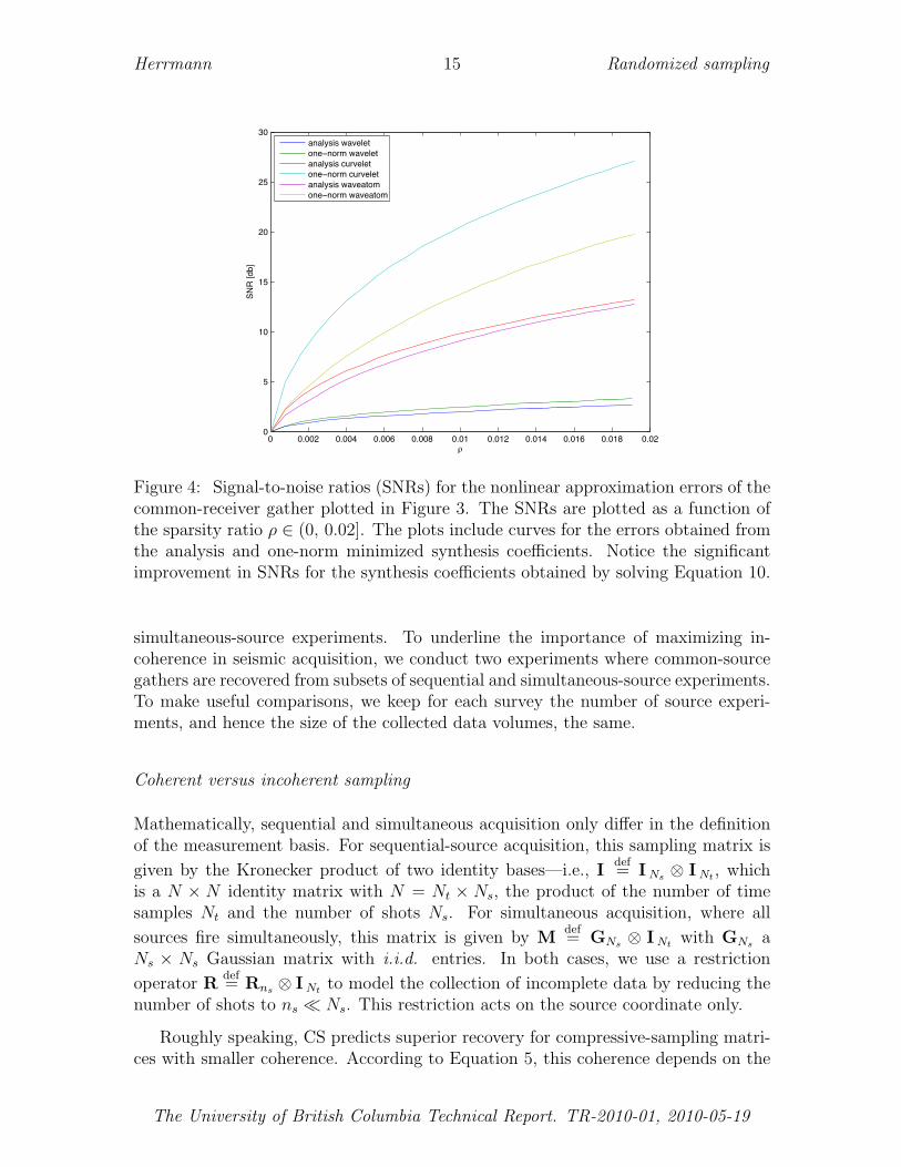
The above definition gives us a metric to compare recovery SNRs of seismic datafor wavelets, curvelets, and wave atoms. We make this comparison on a common-receiver gather (Figure 3) extracted from a Gulf of Suez dataset. Because the currentimplementations of wave atoms (Demanet and Ying, 2007) only support data thatis square, we padded the 178 traces with zeros to 1024 traces. The temporal andspatial sampling interval of the high-resolution data are 0.004s and 25m, respectively.Because this zero-padding biases the ρ, we apply a correction.

Figure 3: Real common-receiver gather from Gulf of a Suez data set.

Our results are summarized in Figure 4 and they clearly show that curvelets leadto rapid improvements in SNR as the sparsity ratio increases. This effect is mostpronounced for synthesis coefficients, benefiting remarkably from sparsity promotion.By comparison, wave atoms benefit not as much, and wavelet even less. This behavioris consistent with the overcompleteness of these transforms, the curvelet transformmatrix has the largest redundancy (a factor of about eight in 2-D) and is therefore thetallest. Wave atoms only have a redundancy of two and wavelets are orthogonal. Sinceour method is based on sparse recovery, this experiment suggests that sparse recoveryfrom subsampling would potentially benefit most from curvelets. However, this is notthe only factor that determines the performance of our compressive-sampling scheme.

Subsampling of shots

Aside from obtaining good reconstructions from small compression ratios, breakingthe periodicity of coherent sampling is paramount to the success of sparse recovery—whether this involves selection of subsets of sources or the design of incoherent



0 0.002 0.004 0.006 0.008 0.01 0.012 0.014 0.016 0.018 0.020

5

10

15

20

25

30

ρ

SN

R [d

b]

analysis waveletone−norm waveletanalysis curveletone−norm curveletanalysis waveatomone−norm waveatom

Figure 4: Signal-to-noise ratios (SNRs) for the nonlinear approximation errors of thecommon-receiver gather plotted in Figure 3. The SNRs are plotted as a function ofthe sparsity ratio ρ ∈ (0, 0.02]. The plots include curves for the errors obtained fromthe analysis and one-norm minimized synthesis coefficients. Notice the significantimprovement in SNRs for the synthesis coefficients obtained by solving Equation 10.

simultaneous-source experiments. To underline the importance of maximizing in-coherence in seismic acquisition, we conduct two experiments where common-sourcegathers are recovered from subsets of sequential and simultaneous-source experiments.To make useful comparisons, we keep for each survey the number of source experi-ments, and hence the size of the collected data volumes, the same.

Coherent versus incoherent sampling

Mathematically, sequential and simultaneous acquisition only differ in the definitionof the measurement basis. For sequential-source acquisition, this sampling matrix is

given by the Kronecker product of two identity bases—i.e., Idef= I Ns ⊗ I Nt , which

is a N × N identity matrix with N = Nt × Ns, the product of the number of timesamples Nt and the number of shots Ns. For simultaneous acquisition, where all

sources fire simultaneously, this matrix is given by Mdef= GNs ⊗ I Nt with GNs a

Ns × Ns Gaussian matrix with i.i.d. entries. In both cases, we use a restriction

operator Rdef= Rns ⊗ I Nt to model the collection of incomplete data by reducing the

number of shots to ns � Ns. This restriction acts on the source coordinate only.

Roughly speaking, CS predicts superior recovery for compressive-sampling matri-ces with smaller coherence. According to Equation 5, this coherence depends on the



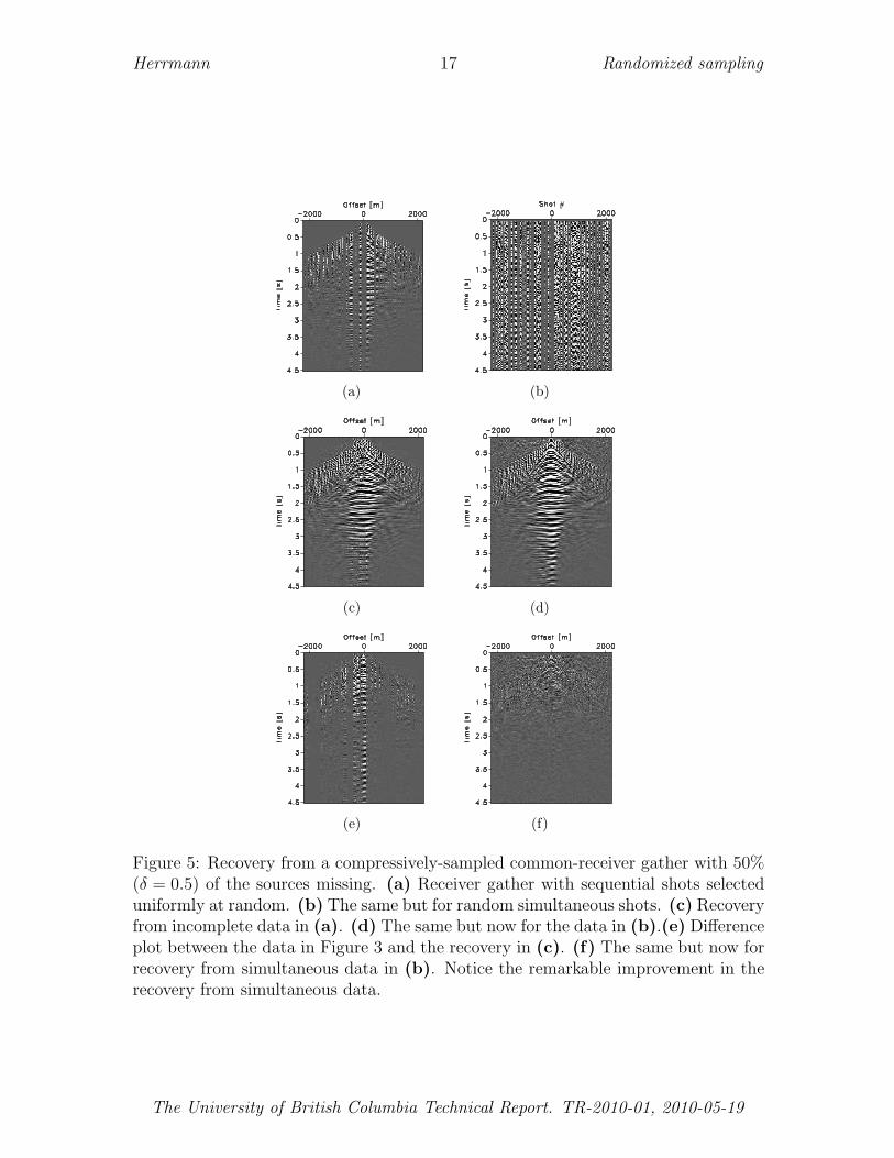
interplay between the restriction, measurement, and synthesis matrices. To make afair comparison, we keep the restriction matrix the same and study the effect of havingmeasurement matrices that are either given by the identity or by a random Gaussianmatrix. Physically, the first CS experiment corresponds to surveys with sequen-tial shots missing. The second CS experiment corresponds to simultaneous-sourceexperiments with simultaneous source experiments missing. Examples of both mea-surements for the real common-receiver gather of Figure 3 are plotted in Figure 5(a)and 5(b), respectively. Both data sets have 50% of the original size. Remember thatthe horizontal axes in the simultaneous experiment no longer has a physical meaning.Notice also that there is no observable coherent crosstalk amongst the simultaneoussources.

Multiplication of orthonormal sparsifying bases by random measurement matricesturns into random matrices with a small mutual coherence amongst the columns. Thisproperty also holds (but only approximately) for redundant signal representationswith synthesis matrices that are wide and have columns that are linearly dependent.This suggests improved performance using random incoherent measurement matrices.To verify this statement empirically, we compare sparse recoveries with Equation 8from data plotted in Figures 5(a) and 5(b).

Despite the fact that simultaneous acquisition with all sources firing simultane-ously may not be easily implementable in practice1, this approach has been appliedsuccessfully to reduce simulation and imaging costs (Herrmann et al., 2009b; Herr-mann, 2009; Lin and Herrmann, 2009a,b). In the “eyeball norm”, the recovery fromthe simultaneous data is as expected clearly superior (cf. Figures 5(c) and 5(d)). Thedifference plots (cf. Figures 5(e) and 5(f)) confirm this observation and show verylittle coherent signal loss for the recovery from simultaneous data. This is consistentwith CS, which predicts improved performance for sampling schemes that are moreincoherent. Because this qualitative statement depends on the interplay between thesampling and the sparsifying transform, we conduct an extensive series of experimentsto get a better idea on the performance of these two different sampling schemes for dif-ferent sparsifying transforms. We postpone our analysis of the quantitative behaviorof the recovery SNRs to after that discussion.

Sparse recovery errors

The examples of the previous section clearly illustrate that randomized samplingis important, and that randomized simultaneous acquisition leads to better recoverycompared to randomized subsampling of sequential sources. To establish this observa-tion more rigorously, we calculate estimates for the recovery error as a function of thesampling ratio δ = n/N by conducting a series of 25 controlled recovery experiments.For each δ ∈ [0.2, 0.8], we generate 25 realizations of the randomized compressive-sampling matrix. Applying these matrices to our common-receiver gather (Figure 3)

1Although one can easily imagine a procedure in the field where a “supershot” is created by somestacking procedure.



(a) (b)

(c) (d)

(e) (f)

Figure 5: Recovery from a compressively-sampled common-receiver gather with 50%(δ = 0.5) of the sources missing. (a) Receiver gather with sequential shots selecteduniformly at random. (b) The same but for random simultaneous shots. (c) Recoveryfrom incomplete data in (a). (d) The same but now for the data in (b).(e) Differenceplot between the data in Figure 3 and the recovery in (c). (f) The same but now forrecovery from simultaneous data in (b). Notice the remarkable improvement in therecovery from simultaneous data.



produces 25 different data sets that are subsequently used as input to sparse recov-ery with wavelets, curvelets, and wave atoms. For each realization, we calculate theSNR(δ) with

SNR(δ) = −20 log‖f − fδ‖‖f‖

, (12)

wherefδ = SH xδ and xδ = arg min

x‖x‖1 subject to Aδx = b.

For each experiment, the recovery of fδ is calculated by solving this optimization

problem for 25 different realizations of Aδ with Aδdef= RδMδS

H , where Rδdef= Rns ⊗

I Nt with δ = ns/Ns. For each simultaneous experiment, we also generate different

realizations of the measurement matrix Mdef= GNs ⊗ I Nt .

¿From these randomly selected experiments, we calculate the average SNRs forthe recovery error, SNR(δ), including its standard deviation. By selecting δ evenlyon the interval δ ∈ [0.2, 0.8], we obtain reasonable reliable estimates with error bars.Results of this exercise are summarized in Figure 6. From these plots it becomesimmediately clear that simultaneous acquisition greatly improves recovery for all threetransforms. Not only are the SNRs better, but the spread in SNRs amongst thedifferent reconstructions is also much less, which is important for quality assurance.The plots validate CS, which predicts improved recovery for increased sampling ratios.Although somewhat less pronounced as for the approximation SNRs in Figure 4, ourresults again show superior performance for curvelets compared to wave atoms andwavelets. This observation is consistent with our earlier empirical findings.

Empirical oversampling ratios

The key factor that establishes CS is the sparsity ratio ρ that is required to recoverwavefields with errors that do not exceed a predetermined nonlinear approximationerror (cf. Equation 11). The latter sets the fraction of largest coefficients that needsto be recovered to meet a preset minimal SNR for reconstruction.

Motivated by Mallat (2009), we introduce the oversampling ratio δ/ρ ≥ 1. For agiven δ, we obtain a target SNR from SNR(δ). Then, we find the smallest ρ for whichthe nonlinear recovery SNR is greater or equal to SNR(δ). Thus, the oversamplingratio δ/ρ ≥ 1 expresses the sampling overhead required by compressive sensing. Thismeasure helps us to determine the performance of our CS scheme numerically. Thesmaller this ratio, the smaller the overhead and the more economically favorable thistechnology becomes compared to conventional sampling schemes.

We calculate for each δ ∈ [0.2, 0.8]

δ/ρ with ρ = inf{ρ : SNR(δ) ≤ SNR(ρ)}. (13)

When the sampling ratio approaches one from below (δ → 1), the data becomesmore and more sampled leading to smaller and smaller recovery errors. To match



0.2 0.4 0.6 0.80

5

10

15

20

25simultaneous wavelet

δ

SN

R [d

B]

0.2 0.4 0.6 0.80

5

10

15

20

25uniform random wavelet

δ

SN

R [d

B]

0.2 0.4 0.6 0.80

5

10

15

20

25simultaneous curvelet

δ

SN

R [d

B]

0.2 0.4 0.6 0.80

5

10

15

20

25uniform random curvelet

δ

SN

R [d

B]

0.2 0.4 0.6 0.80

5

10

15

20

25simultaneous waveatom

δ

SN

R [d

B]

0.2 0.4 0.6 0.80

5

10

15

20

25uniform random waveatom

δ

SN

R [d

B]

Figure 6: SNRs (cf. Equation 12) for nonlinear sparsity-promoting recovery fromcompressively sampled data with 20%− 80% of the sources missing (δ ∈ [0.2, 0.8]).The results summarize 25 experiments for 25 different values of δ ∈ [0.2, 0.8]. Theplots include estimates for the standard deviations. From these results, it is clear thatsimultaneous acquisition (results in the left column) is more conducive to sparsity-promoting recovery. Curvelet-based recovery seems to work best, especially towardshigh percentages of data missing.



this decreasing error, the sparsity ratio ρ → 1 and consequently we can expect thisoversampling ratio to go to one, δ/ρ → 1.

Remember that in the CS paradigm, acquisition costs grow with the permissiblerecovery SNR that determines the sparsity ratio. Conversely, the costs of conventionalsampling grow with the size of the sampling grid irrespective of the transform-domaincompressibility of the wavefield, which in higher dimensions proves to be a majordifficulty.

The numerical results of our experiments are summarized in Figure 7. Our calcula-tions use empirical SNRs for both the approximation errors of the synthesis coefficientsas a function of ρ and the recovery errors as a function of δ. The estimated curveslead to the following observations. First, as the sampling ratio increases the oversam-pling ratio decreases, which can be understood because the recovery becomes easierand more accurate. Second, recoveries from simultaneous data have significantly lessoverhead and curvelets outperform wave atoms, which in turn perform significantlybetter than wavelets. All curves converge to the lower limit (depicted by the dashedline) as δ → 1. Because of the large errorbars in the recovery SNRs (cf. Figure 6),the results for the recovery from missing sequential sources are less clear. However,general trends predicted by CS are also observable for this type of acquisition, butthe performance is significantly worse than for recovery with simultaneous sources.Finally, the observed oversampling ratios are reasonable for both curvelet and waveatoms.

AN ACADEMIC CASE STUDY

Now that we established that high SNR’s are achievable with modest oversamplingratios, we study the performance of our recovery algorithm on a seismic line fromthe Gulf of Suez by comparing two simultaneous-source scenarios with coincidentsource-receiver positions:

• ‘Land’ acquisition with random amplitude encoding: Here, sequen-tial impulsive sources are replaced by impulsive simultaneous ‘phase-encoded’sources. Mathematically, simultaneous measurements are obtained by replacingthe sampling matrix for the sources—normally given by identity matrix—by ameasurement matrix obtained by phase encoding along the source coordinate.Following Romberg (2009) and Herrmann et al. (2009b), we define the measure-ment matrix by the following Kronecker product

Mdef=

I ⊗

Gaussian matrix︷︸︸︷diag (η)F∗

s diag(eiθ

)Fs⊗I

. (14)

In this expression, conventional sampling, which corresponds to the action of theidentity matrix I, is replaces by a ’random phase encoding’ consisting of apply-ing a Fourier transform along the source coordinate (Fs), followed by uniformly



0.2 0.4 0.6 0.8

1020304050607080

1

simultaneous wavelet

δ

δ/ρ

0.2 0.4 0.6 0.8

50

100

150

200

uniform random wavelet

δ

δ/ρ

0.2 0.4 0.6 0.8123456789

simultaneous curvelet

δ

δ/ρ

0.2 0.4 0.6 0.8

102030405060

uniform random curvelet

δ

δ/ρ

0.2 0.4 0.6 0.8

2468

101214

simultaneous waveatom

δ

δ/ρ

0.2 0.4 0.6 0.8

10203040506070

uniform random waveatom

δ

δ/ρ

Figure 7: Oversampling ratio δ/ρ as a function of the sampling ratio δ (cf. Equa-tion 13) for sequential- and simultaneous-source experiments. As expected, the over-head is smallest for simultaneous acquisition and curvelet-based recovery.



drawn random phase rotations θ ∈ [0, π], an inverse Fourier transform (F∗s ),

and a multiplication by a a random sign vector (i.e., multiplication by diag (η)with (η) ∈ N(0, 1)). As shown by Romberg (2009), the combined action of theseoperations corresponds to the action of a Gaussian matrix at reduced compu-tational costs (see also Herrmann et al., 2009b). Application of this matrixto a conventionally-sampled seismic line turns sequential impulsive source intoa simultaneous ‘supershot’ where all sources fire simultaneously with weightsdrawn from a single Gaussian distribution. As before, the restriction operatorselects a subset of n′s ‘supershots’ generated by different randomly-weighted si-multaneous sources. After restriction along the source coordinate, the samplingmatrix has an aspect(or undersampling) ratio of δ = n′s/ns. An example of thistype of sampling, resulting in a seismic line consisting of n′s � ns supershots,is included in Figure 8. In this Figure, ns single impulsive-source experiments(8(a)) become n′s simultaneous-source experiments (juxtapose Figure 8(a) and8(c)). While this sort of sampling is perhaps physically unrealizable—i.e., wetypically do not have large numbers of vibroseis trucks available—it gives usthe most favorable recovery conditions from the compressive-sensing perspec-tive. Therefore, our ‘Land’ acquisition will serve as a benchmark with whichwe can compare alternative and physically more realistic acquisition scenarios.

• ‘Marine’ acquisition with random-time dithering: Here, sequential ac-quisition with a single airgun is replaced by continuous acquisition with multipleairguns that fire continuously at random times and at random locations. In thisscenario, a seismic line is mapped into a single long ‘supershot’. Mathematically,this type of acquisition is represented by the following sampling operator

RMdef= [I ⊗T] . (15)

In this expression, the linear operator T turns sequential recordings (8(b)) withsynchronized impulsive shots (Figure 8(a)) into continuous recordings with n∗simpulsive sources firing at random positions (Figure 8(e)), selected uniformly-random from [1 · · ·ns] discrete source indices and from discrete random timeindices, selected uniformly from (0 · · · (n∗s − 1)× nt)] time indices. Note that Tacts both on the shot and the time coordinate. The resulting data is one longsupershot’ that contains a superposition of n∗s impulsive shots. For plottingreasons, we reshaped in Figure 8(f) this long record into multiple shorter records.Notice that this type of ‘Marine’ acquisition is physically realizable as long asthe number of simultaneous sources involved is limited.

Aside from mathematical factors, such as the mutual coherence (cf. Equation 5)that determines the recovery quality, there are also economical factors to consider. Forthis purpose, Berkhout (2008) proposed two performance indicators, which quantifythe cost savings associated with simultaneous and continuous acquisition. The firstmeasure compares the number of sources involved in conventional and simultaneous



acquisition and is expressed in terms of the source-density ratio

SDR =number of sources in the simultaneous survey

number of sources in the conventional survey. (16)

For ‘Land data’ acquisition, this quantity equals SDRLand = (ns×n′s)/ns = n′s and for‘Marine data’ SDRMarine = n∗s/ns. Remember that the number of sources refers thenumber of sources firing and not the number of source experiments. Clearly, ‘Land’acquisition has a significant higher SDR.

Aside from the number of sources, the cost of acquisition is also determined bysurvey-time ratio

STR =time of the conventional sequential survey

time of the continuous and simultaneous recording. (17)

Ignoring overhead in sequential shooting, this quantity equals STRLand = ns/n′s in

the first and STRMarine = ns×T0/T with T0 the time of a single sequential experimentand T the total survey time of the continuous recording. The overall economic per-formance is measured by the product of these two ratios. For ‘Land’ acquisition thisproduct is proportional to ns and for ‘Marine’ acquisition proportional to n∗s × T0/T .

As we have seen from our discussion on compressive sensing, recovery dependson the mutual coherence of the sampling matrix. So, the challenge really lies inthe design of acquisition scenarios that obtain the lowest mutual coherence whilemaximizing the above two economic performance indicators. To get a better insightin how these factors determine the quality of recovered data, we conduct a series ofexperiments by simulating possible alternative acquisition strategies on a perviouslytraditionally recorded real seismic line.

First, we simulate ‘Land’ data for δ = 0.5 (64 simultaneous source experimentswith all sources firing) and study the recovery based on 2-D and 3-D curvelets. Theformer is based on a 2-D discrete curvelet transform along the source and receivercoordinates, and the discrete wavelet transform along the remaining time coordinate:

Sdef= C2 ⊗W. (18)

We conduct a similar experiment for the ‘Marine case’. In this case, we randomlyselect 128 shots from the total survey time T = δ × (ns − 1)× T0, yielding the sameaspect ratio for the sampling matrix.

Figures 9 and 10 summarize the results for ‘Land’ and ‘Marine’ acquisition usingrecoveries based on the 2-D and 3-D curvelet transform. The following observationscan be made. First, it is clear that accurate recovery is possible by solving an `1

optimization problem using SPG`1 (Berg and Friedlander, 2008) while limiting thenumber of iterations for the 2-D case to 500 and the 3-D case to 200. Second, therecovery results for 3-D recovery of ‘Land’ data show and improvement 1.3 dB byexploiting 3-D structure of the wavefronts. Similarly, we find an improvement of



3.9 dB for the ‘Marine’ case. Both observations can be explained by the fact that the3-D curvelet transforms attains higher sparsity because it explores continuity of thewavefield along all three coordinate axes. Second, ‘Land’ acquisition clearly favorsrecovery by curvelet-domain sparsity promotion compared to ‘Marine’ acquisition.This is true despite the fact that the subsampling ratio, i.e., the aspect ratio of thesampling matrices, are the same. Clearly this difference lies in the mutual coherenceof the sampling matrix. The columns of the sampling matrix for ‘Land’ acquisitionare more incoherent and hence more independent and this favors recovery. These ob-servations are confirmed by the SNRs, which for ‘Land’ acquisition equal 10.3 dB and11.6dB, for the 2-D/3-D recovery, respectively, and 7.2 dB and 11.1 dB, for ‘Marine’acquisition.

Unfortunately, recovery quality is not the only consideration. The economicsexpressed by the SDR and STR also play a role. In the above setting, the ‘Land’acquisition has a SDR = 64 and STR = 2 while the ‘Marine’ acquisition has SDR = 1and STR = 2. Clearly, the SDR for land acquisition may not be realistic.

DISCUSSION

The presented results illustrate that we are at the cusp of exciting new developmentswhere acquisition workflows are no longer impeded by subsampling related artifacts.Instead, we arrive at acquisition schemes that control these artifacts. We accomplishby applying the following design principles: (i) randomize—break coherent aliasesby introducing randomness, e.g. by designing randomly perturbed acquisition grids,or by designing randomized simultaneous sources; and (ii) sparsify—utilize sparsify-ing transforms in conjunction with sparsity-promoting programs that separate signaland subsampling artifacts and that restore amplitudes. The implications of random-ized incoherent sampling go far beyond the examples presented here. For instance,our approach is applicable to land acquisition for physically realizable sources (Krohnand Neelamani, 2008; Romberg, 2009) and can be used to compute solutions to wave-field simulations (Herrmann et al., 2009b) and to compute full waveform inversion(Herrmann et al., 2009a) faster. Because randomized sampling is linear (Bobin et al.,2008), wavefield reconstructions and processing can be carried out incrementally asmore compressive data becomes available.

Indeed, compressive sensing offers enticing perspectives towards the design of fu-ture Land and Marine acquisition systems. In order for this technology to becomesuccessful the following issues need to be addressed, namely the performance of re-covery

• from field data including all its idiosyncrasies. This will require an concertedeffort from practitioners in the field and theoreticians. For Marine acquisition,recent work by Moldoveanu (2010) has shown early indications that randomizedjittered sampling leads to improved imaging.



• from discrete data with quantization errors. Addressing this issue calls forintegration of digital-to-analog conversion into compressive and recent progresshas been made in this area (see e.g. Gunturk et al., 2010);

• from Land data that has the imprint of statics. Addressing this issue will beessential because severe static effects may adversely affect transform-domainsparsity on which recovery from compressive-sampled data relies.

At the UBC Seismic Laboratory for Imaging and Modelling (SLIM), we hope toreport progress on these important topics in future publications.

CONCLUSIONS

Following ideas from compressive sensing, we made the case that seismic wavefieldscan be reconstructed with a controllable error from randomized subsamplings. Bymeans of carefully designed numerical experiments on synthetic and real data, weestablished that compressive sensing can indeed successfully be adapted to seismicdata acquisition, leading to a new generation of randomized acquisition and processingmethodologies.

With carefully designed experiments and the introduction of performance mea-sures for nonlinear approximation and recovery errors, we established that curveletsperform best in recovery, closely followed by wave atoms, and with wavelets com-ing in as a distant third, which is consistent with the directional nature of seismicwavefronts. This finding is remarkable for the following reasons: (i) it underlines theimportance of sparsity promotion, which offsets the “costs” of redundancy and (ii)it shows that the relative sparsity ratio effectively determines the recovery perfor-mance rather than the absolute number of significant coefficients. Our observationof significantly improved recovery for simultaneous-source acquisition also confirmspredictions of compressive sensing. Finally, our analysis showed that accurate recov-eries are possible from compressively sampled data volumes that exceed the size ofconventionally compressed data volumes by only a small factor.

The fact that compressive sensing combines sampling and compression in a sin-gle linear encoding step has profound implications for exploration seismology thatinclude: a new randomized sampling paradigm, where the cost of acquisition areno longer dominated by resolution and size of the acquisition area, but by the de-sired reconstruction error and transform domain sparsity of the wavefield, and a newparadigm for randomized processing and inversion, where dimensionality reductionswill allow us to mine high-dimensional data volumes for information in ways, whichpreviously, would have been computationally infeasible.


http://slim.eos.ubc.ca/


ACKNOWLEDGMENTS

This paper was written as a follow up to the first author’s presentation during the“Recent advances and Road Ahead” session at the 79th annual meeting of the So-ciety of Exploration Geophysicists. I would like to thank the organizers of thissession Dave Wilkinson and Masoud Nikravesh for their invitation. I also wouldlike to thank Dries Gisolf and Eric Verschuur of the Delft University of Technol-ogy for their hospitality during my sabbatical and Gilles Hennenfent for preparingsome of the figures. This publication was prepared using CurveLab (curvelet.org),a toolbox implementing the Fast Discrete Curvelet Transform, WaveAtom a tool-box implementing the Wave Atom transform (http://www.waveatom.org/), Mada-gascar (rsf.sf.net), a package for reproducible computational experiments, SPG`1

(cs.ubc.ca/labs/scl/spgl1), SPOT (http://www.cs.ubc.ca/labs/scl/spot/),a suite of linear operators and problems for testing algorithms for sparse signal re-construction, and pSPOT, SLIM’s parallel extension of SPOT. FJH was in part fi-nancially supported by NSERC Discovery Grant (22R81254) and by CRD GrantDNOISE II 375142-08. The industrial sponsors of the Seismic Laboratory for Imag-ing and Modelling (SLIM) BG Group, BP, Chevron, ConocoPhillips, Petrobras, TotalSA, and WesternGeco are also gratefully acknowledged.


curvelet.org

http://www.waveatom.org/

rsf.sf.net

cs.ubc.ca/labs/scl/spgl1

http://www.cs.ubc.ca/labs/scl/spot/

http://www.nserc.gc.ca/index.htm

http://slim.eos.ubc.ca/index.php?module=articles&func=display&catid=55&aid=361

http://www.bg-group.com/

http://www.bp.com/

http://www.chevron.com/

http://www.conocophillips.com/

http://www.petrobras.com/

http://www.total.com/

http://www.total.com/

http://www.westerngeco.com/


REFERENCES

Abma, R., and N. Kabir, 2006, 3D interpolation of irregular data with a POCSalgorithm: Geophysics, 71, E91–E97.

Berg, E. v., and M. P. Friedlander, 2008, Probing the Pareto frontier for basis pursuitsolutions: Technical Report 2, Department of Computer Science, University ofBritish Columbia.

Berkhout, A. J., 2008, Changing the mindset in seismic data acquisition: The LeadingEdge, 27, 924–938.

Bleistein, N., J. Cohen, and J. Stockwell, 2001, Mathematics of MultidimensionalSeismic Imaging, Migration and Inversion: Springer.

Bobin, J., J. Starck, and R. Ottensamer, 2008, Compressed sensing in astronomy:IEEE J. Selected Topics in Signal Process, 2, 718–726.

Candes, E., J. Romberg, and T. Tao, 2006, Stable signal recovery from incompleteand inaccurate measurements: Comm. Pure Appl. Math., 59, 1207–1223.

Candes, E. J., and L. Demanet, 2005, The curvelet representation of wave propagatorsis optimally sparse: Comm. Pure Appl. Math, 58, 1472–1528.

Candes, E. J., L. Demanet, D. L. Donoho, and L. Ying, 2006a, Fast discrete curvelettransforms: Multiscale Modeling and Simulation, 5, 861–899.

Candes, E. J., J. Romberg, and T. Tao, 2006b, Robust uncertainty principles: Exactsignal reconstruction from highly incomplete frequency information: IEEE Trans-actions on Information Theory, 52, 489 – 509.

Canning, A., and G. H. F. Gardner, 1996, Regularizing 3-d data sets with dmo: 61,1103–1114.

Demanet, L., and L. Ying, 2007, Wave atoms and sparsity of oscillatory patterns:Applied and Computational Harmonic Analysis, 23, 368–387.

Donoho, D., A. Maleki, and A. Montanari, 2009, Message passing algorithms forcompressed sensing: Proceedings of the National Academy of Sciences.

Donoho, D., and J. Tanner, 2009, Observed universality of phase transitions in high-dimensional geometry, with implications for modern data analysis and signal pro-cessing: Philosophical Transactions of the Royal Society A: Mathematical, Physicaland Engineering Sciences, 367, 4273.

Donoho, D. L., 2006a, Compressed sensing: IEEE Trans. Inform. Theory, 52, 1289–1306.

——–, 2006b, Compressed sensing: IEEE Transactions on Information Theory, 52,1289 – 1306.

Donoho, D. L., and X. Huo, 2001, Uncertainty principles and ideal atomic decompo-sition: IEEE Transactions on Information Theory, 47, 2845–2862.

Donoho, D. L., and B. F. Logan, 1992, Signal Recovery and the Large Sieve: SIAMJournal on Applied Mathematics, 52, 577–591.

Donoho, P., R. Ergas, and R. Polzer, 1999, Development of seismic data compressionmethods for reliable, low-noise performance: SEG International Exposition and69th Annual Meeting, 1903–1906.

Fomel, S., 2003, Theory of differenctial offset continuation: 68, 718–732.Fomel, S., J. G. Berryman, R. G. Clapp, and M. Prucha, 2002, Iterative resolution



(a) (b)

(c) (d)

0 500 1000 1500 2000 2500 3000 3500

0

10

20

30

40

50

60

70

Source Position (m)

Tim

e (s

)

(e) (f)

Figure 8: Different acquisition scenarios. (a) Impulsive sources for conventionalsequential acquisition, yielding 128 shot records for 128 receivers and 512 time sam-ples. (b) Corresponding fully sampled sequential data. (c) Simultaneous sources for‘Land’ acquisition with 64 simultaneous-source experiments. Notice that all shots firesimultaneously in this case. (d) Corresponding compressively sampled land data. (e)Simultaneous sources for ‘Marine’ acquisition with 128 sources firing at random timesand locations during a continuous total ’survey’ time of T = 262s. (f) Corresponding‘Marine’ data plotted as a conventional seismic line.



(a) (b)

(c) (d)

Figure 9: Sparsity-promoting recovery with δ = 0.5 with the 2-D curvelet transforms.(a) 2-D curvelet-based recovery from ‘Land’ datat (10.3 dB). (b) The correspondingdifference plot. (c) 2-D curvelet-based recovery from ‘Marine’ datat (7.2 dB). (d)Corresponding difference plot. Notice the improvement in recovery from ‘Land’ data.



(a) (b)

(c) (d)

Figure 10: Sparsity-promoting recovery with δ = 0.5 with the 3-D curvelet transforms.(a) 3-D curvelet-based recovery from ‘Land’ data (11.6 dB). (b) The correspondingdifference plot. (c) 3-D curvelet-based recovery from ‘Marine’ data (11.1 dB). (d)Corresponding difference plot. Notice the improvement in recovery compared to 2-Dcurvelet based recovery.



estimation in least-squares Kirchoff migration: Geophys. Pros., 50, 577–588.Gunturk, S., A. Powell, R. Saab, and O. Yılmaz, 2010, Sobolev duals for random

frames and Sigma-Delta quantization of compressed sensing measurements: Arxivpreprint arXiv:1002.0182.

Hale, D., 1995, DMO processing: Geophysics Reprint Series.Harlan, W. S., J. F. Claerbout, and F. Rocca, 1984, Signal/noise separation and

velocity estimation: Geophysics, 49, 1869–1880.Hennenfent, G., and F. J. Herrmann, 2008, Simply denoise: wavefield reconstruction

via jittered undersampling: Geophysics, 73.Herrmann, F. J., 2009, Compressive imaging by wavefield inversion with group spar-

sity: SEG Technical Program Expanded Abstracts, SEG, SEG, 2337–2341.Herrmann, F. J., U. Boeniger, and D. J. Verschuur, 2007, Non-linear primary-multiple

separation with directional curvelet frames: Geophysical Journal International,170, 781–799.

Herrmann, F. J., Y. A. Erlangga, and T. Lin, 2009a, Compressive sensing applied tofull-waveform inversion.

——–, 2009b, Compressive simultaneous full-waveform simulation: Geophysics, 74,A35.

Herrmann, F. J., and G. Hennenfent, 2008, Non-parametric seismic data recoverywith curvelet frames: Geophysical Journal International, 173, 233–248.

Herrmann, F. J., P. P. Moghaddam, and C. C. Stolk, 2008, Sparsity- and continuity-promoting seismic imaging with curvelet frames: Journal of Applied and Compu-tational Harmonic Analysis, 24, 150–173. (doi:10.1016/j.acha.2007.06.007).

Krohn, C., and R. Neelamani, 2008, Simultaneous sourcing without compromise:Rome 2008, 70th EAGE Conference & Exhibition, B008.

Levy, S., D. Oldenburg, and J. Wang, 1988, Subsurface imaging using magnetotelluricdata: Geophysics, 53, 104–117.

Lin, T., and F. J. Herrmann, 2009a, Designing simultaneous acquisitions with com-pressive sensing: Presented at the EAGE Technical Program Expanded Abstracts,EAGE.

——–, 2009b, Unified compressive sensing framework for simultaneous acquisitionwith primary estimation: SEG Technical Program Expanded Abstracts, SEG,3113–3117.

Malcolm, A. E., M. V. de Hoop, and J. A. Rousseau, 2005, The applicability ofdmo/amo in the presence of caustics: Geophysics, 70, S1–S17.

Mallat, S. G., 2009, A Wavelet Tour of Signal Processing: the Sparse Way: AcademicPress.

Moldoveanu, N., 2010, Random sampling: A new strategy for marine acquisition:SEG, Expanded Abstracts, 29, 51–55.

Oldenburg, D. W., S. Levy, and K. P. Whittall, 1981, Wavelet estimation and decon-volution: Geophysics, 46, 1528–1542.

Rauhut, H., K. Schnass, and P. Vandergheynst, 2008, Compressed sensing and re-dundant dictionaries: IEEE Trans. Inform. Theory, 54, 2210–2219.

Romberg, J., 2009, Compressive sensing by random convolution: SIAM Journal onImaging Sciences, 2, 1098–1128.



Sacchi, M. D., T. J. Ulrych, and C. Walker, 1998, Interpolation and extrapolationusing a high-resolution discrete Fourier transform: IEEE Trans. Signal Process.,46, 31–38.

Sacchi, M. D., D. R. Velis, and A. H. Cominguez, 1994, Minimum entropy deconvo-lution with frequency-domain constraints: Geophysics, 59, 938–945.

Santosa, F., and W. Symes, 1986, Linear inversion of band-limited reflection seismo-gram: SIAM J. of Sci. Comput., 7.

Smith, H. F., 1998, A Hardy space for Fourier integral operators.: J. Geom. Anal.,8, 629–653.

Spitz, S., 1999, Pattern recognition, spatial predictability, and subtraction of multipleevents: The Leading Edge, 18, 55–58.

Tang, G., J. Ma, and F. Herrmann, 2009, Design of two-dimensional randomized sam-pling schemes for curvelet-based sparsity-promoting seismic data recovery.: Tech-nical Report TR-2009-03, the University of British Columbia.

Taylor, H. L., S. Banks, and J. McCoy, 1979, Deconvolution with the `1 norm: Geo-physics, 44, 39.

Trad, D., T. Ulrych, and M. Sacchi, 2003, Latest views of the sparse radon transform:Geophysics, 68, 386–399.

Trad, D. O., 2003, Interpolation and multiple attenuation with migration operators:Geophysics, 68, 2043–2054.

Ulrych, T. J., and C. Walker, 1982, Analytic minimum entropy deconvolution: Geo-physics, 47, 1295–1302.

Xu, S., Y. Zhang, D. Pham, and G. Lambare, 2005, Antileakage Fourier transformfor seismic data regularization: Geophysics, 70, V87 – V95.

Zwartjes, P. M., and M. D. Sacchi, 2007a, Fourier reconstruction of nonuniformlysampled, aliased data: Geophysics, 72, V21–V32.

——–, 2007b, Fourier reconstruction of nonuniformly sampled, aliased seismic data:Geophysics, 72, V21–V32.


compressive sensing in seismic exploration: an outlook … · compressive sensing in seismic...

Documents