Instructions for use

Title Comprehensive Study of the Enhancement of Interplate Coupling in Adjacent Segments after Recent MegathrustEarthquakes

Author(s) Yuzariyadi, Mohammad

Citation 北海道大学. 博士(理学) 甲第14369号

Issue Date 2021-03-25

DOI 10.14943/doctoral.k14369

Doc URL http://hdl.handle.net/2115/81976

Type theses (doctoral)

File Information Mohammad_Yuzariyadi.pdf

Hokkaido University Collection of Scholarly and Academic Papers : HUSCAP

i

Comprehensive Study of the Enhancement of Interplate Coupling

in Adjacent Segments after Recent Megathrust Earthquakes

(最近のプレート境界地震に続いて隣接セグメントで

生じたプレート間固着強化に関する包括的研究)

By

Mohammad Yuzariyadi

Supervisor: Prof. Kosuke Heki

A dissertation submitted in partial fulfillment

of the requirements for the degree of

Doctor of Philosophy

Department of Natural History Science

Graduate School of Science, Hokkaido University

March 2021

ii

Abstract

In general, the concept of a seismic cycle, especially in subduction zones, consists

of three phases: interseismic, coseismic, and postseismic. These three phases can

be observed through surface crustal movement observations with Global

Navigation Satellite System (GNSS) because these three phases have different

directions of velocities. During the interseismic stage, all GNSS stations on an arc

move landward; during the coseismic stage, they jump seaward, and during the

postseismic stage, they slowly move seaward and eventually return to the

interseismic regime. During the postseismic phase, the deformation caused by the

viscoelastic relaxation results in prolonged seaward movement.

Apart from such a classical concept of postseismic seaward movement, several

previous studies have also found increased landward surface velocities in the early

postseismic stages, especially in segments adjacent along-trench to the megathrust

ruptures.

Such cases have been found for the 2003 Tokachi-oki and the 2011 Tohoku-oki

earthquakes, NE Japan. A similar increase of landward velocities was reported for

the segments to the north of the rupture of the 2010 Maule earthquake, Chile. I

utilize available GNSS data to find such changes for six megathrust earthquakes in

four subduction zones, including NE Japan, central and northern Chile, Sumatra,

and Mexico to investigate their common features. My study showed that such

increase, ranging from a few mm/yr to ~1 cm/yr, also appeared in adjacent segments

of the 2014 Iquique (Chile), the 2007 Bengkulu (Sumatra), and the 2012 Oaxaca

(Mexico) earthquakes in addition to the three previously known cases.

The region of the increased landward movements usually extends with spatial decay

iii

and reach the distance comparable to the along-strike fault length. On the other hand,

the temporal decay of the increased velocity is not clear at present. The degree of

increase seems to depend on the earthquake magnitude, and possibly scales with

the average fault slip in the earthquake. This is consistent with the simple two-

dimensional model proposed earlier to attribute the phenomenon to the enhanced

coupling caused by accelerated slab subduction. However, these data are not strong

enough to rule out other possibilities.

In addition to the information above, I also investigated possible increase in

background seismicity following the 2011 Tohoku-oki and the 2010 Maule

earthquakes in the regions where GNSS stations showed enhanced coupling. Recent

studies suggest that relative plate velocity correlates positively with the seismicity

and predict that background seismicity increases where plate convergence

accelerates. There, I found a moderate but significant increase in seismicity of

~10%, somewhat smaller than the rates of increased landward velocities.

iv

Acknowledgments

ة ول حول ل إل قو ٱلعظيم ٱلعلي بٱلل

I would like to express my special thanks to my supervisor, Prof Kosuke Heki,

who patiently encouraged and guided me. This research topic is new for me, yet

while I spent four years working with him, Heki-sensei always answered my

question without making me feel inferior.

This study was fully financed by the Indonesia Endowment Fund for Education

(LPDP) scholarship. I am grateful for the opportunity they gave me to pursue

study at Hokkaido University.

I would also thank Dr. Kei Katsumata, whom I visited several times to discuss the

ETAS program and its results.

I also would like to thank Prof. Masato Furuya, Dr. Youichiro Takada, and Prof.

Takahashi Hiroaki for their constructive comments.

I'd like to express my gratitude to my family, especially My father and mother,

who always send their prayers so that this Ph.D.-journey went well. And of

course, for my wife and her patience, I really thank her for supporting me all these

times.

v

Table of Contents

Abstract ............................................................................................................... i Acknowledgments ................................................................................................ iv Table of Contents ................................................................................................... v Chapter 1: Introduction........................................................................................ 1

1.1 Backgrounds ............................................................................................ 1

1.1.1 Classical Concept of Seismic Cycle .................................................. 1

1.1.2 Postseismic Deformation Studies ..................................................... 2

1.1.3 Viscoelastic Relaxation .................................................................... 4

1.2 A Brand-New Process in the Earthquake Cycle ....................................... 6

1.3 Previous works ........................................................................................... 10

1.4 Objectives ................................................................................................... 12

Chapter 2: Data and Method ............................................................................. 16 2.1 GNSS Data.................................................................................................. 16

2.1.1 GNSS Data in Japan ...................................................................... 18

2.1.2 GNSS Data in Sumatra ................................................................. 19

2.1.3 GNSS Data in South and Middle America .................................... 22

2.1.4 Time series analysis strategy ......................................................... 26

2.2 Method for acceleration analysis .............................................................. 30

2.3 Slab acceleration model by Heki and Mitsui (2013) ............................... 33

2.4 Subduction zones and slab data interpretation ...................................... 36

Chapter 3: Enhanced interplate coupling after various megathrust

earthquakes ....................................................................................... 41 3.1 The cases in Japan ..................................................................................... 41

3.1.1 Tectonic setting in Northeast Japan .............................................. 41

3.1.2 The 2011 Tohoku-oki earthquake (Mw 9.0) ................................... 42

3.1.3 The 2003 Tokachi-oki Earthquake (Mw 8.3) .................................. 49

3.2 The cases in Chile ...................................................................................... 55

vi

3.2.1 Tectonic setting in Central and Northern Chile ............................ 55

3.2.2 The 2010 Maule Earthquake (Mw 8.8) ........................................... 57

3.2.3 The 2014 Iquique Earthquake (Mw 8.2) ......................................... 61

3.3 The case in Sumatra .................................................................................. 65

3.3.1 Tectonic setting in Southwest Sumatra.......................................... 65

3.3.2 The 2007 Bengkulu Earthquake (Mw 8.4) ...................................... 66

3.4 The case in Mexico ..................................................................................... 69

3.4.1 Tectonic Setting of Mexico ............................................................ 69

3.4.2 The 2012 Oaxaca Earthquake (Mw 7.4) ......................................... 70

Chapter 4: Discussion ......................................................................................... 72 4.1 Overview of the six cases ........................................................................... 72

4.2 Spatial decay of the enhanced coupling ................................................... 74

4.3 Temporal decay of the enhanced coupling .............................................. 77

4.4 Forearc station velocities and slab velocities ........................................... 81

4.5 Comparison of the data with the slab acceleration model (Heki and

Mitsui, 2013) ..................................................................................................... 82

Chapter 5: Change in Seismicity ....................................................................... 89 5.1 Previous Studies ......................................................................................... 89

5.2 Seismicity data ........................................................................................... 90

5.3 Seismicity declustering .............................................................................. 93

Chapter 6: Conclusion ........................................................................................ 98 References .......................................................................................................... 101

1

Chapter 1: Introduction

1.1 Backgrounds

1.1.1 Classical Concept of Seismic Cycle

Earthquakes occur due to the presence of locked plates interfaces, resulting in

lithospheric stress and strain. Accumulated compressional and extensional strain

that exceeds the elasticity limit of rock is released as fault dislocations, which let

seismic waves to radiate from the faults.

Earthquakes that occurred at a certain time often recur after a while. Such

cycles continue over thousands of years and are called the “earthquake cycle

(seismic cycle)” (e.g. see Broerse, 2012). Records of past earthquake cycles can be

found from old documents recording them or through geological observations such

as stratigraphic studies of rocks, coral reefs, paleo-tsunami, and paleo-seismology

(e.g. Natawidjaja et al., 2006).

Advent of space geodetic techniques such as Global Navigation Satellite

System (GNSS) since 1990s established the classical concept of crustal movement

in an earthquake cycle. According to this concept, forearc movements at convergent

plate boundaries over seismic cycle are characterized by the alternation of slow

interseismic landward movement and coseismic trenchward jump. The interseismic

movements reflect interplate coupling that accumulates strain toward the next

interplate earthquakes. The coseismic jumps correspond to the release of such strain.

2

Following coseismic jumps, we often observe transient postseismic crustal

deformation. Its mechanisms can be divided into 3 types, that is:

1. Poroelastic rebound; deformation that occurs due to fluid moving from a

place with high pressure to a place with low pressure driven by compression

(e.g. Jónsson et al. 2003).

2. Afterslip; the slow displacement that occurs due to slow continuing slips of

the fault (e.g. Heki et al., 1997).

3. Viscoelastic relaxation; relaxation of shear stress coming from viscous flow

in the asthenosphere (e.g. Wang et al., 2012).

The three mechanisms differ both in space and time domains. Peltzer et al.

(1998) showed that poroelastic deformation occurred over a short period of time,

usually within a few months after the main earthquake and/or within small distance

from the fault, say 10-20 km. In addition to it, crustal deformation due to afterslip

and viscoelastic relaxation occur over a larger spatial and temporal scale.

Deformation caused by viscoelastic relaxation mechanism may continue for

decades after a megathrust earthquake. A typical example can be found in the

postseismic deformations of the 1964 Alaska earthquake (Mw 9.2) lasting more than

30 years (Suito and Freymueller, 2009).

1.1.2 Postseismic Deformation Studies

In the 1980s, Thatcher and Rundle (1984) developed a two-dimensional model

to explain the long-term deformations recorded in the Nankai subduction zone,

southwest Japan. They concluded that three main stages exist in crustal deformation

of every major earthquake; interseismic, coseismic, and postseismic. Research in

3

later years suggested that the asthenospheric viscosity in subduction zones is in the

order of 1019 Pa∙s, lower than the global average of 1020–1021 Pa∙s (Wang, 2007).

Important findings since the 1980s include:

1. The importance of viscosity of the wedge mantle,

2. Viscoelastic effect consists of short- and long-term components,

3. Existence of afterslips,

4. Magnitude-dependent relaxation times.

Another development is that the previously used viscosity value ~1019 Pa∙s was

updated. The viscosity used to explain satellite gravity observations after the 2004

Sumatra earthquake was 1018–1019 Pa∙s (Panet et al., 2010; Han et al., 2008).

In the 1980s, postseismic relaxation time constant could not be constrained

with sufficient accuracy until the development of Global Positioning System (GPS),

the first GNSS developed in America. This technology revolutionized the

measurement of crustal deformation. Since the early 1990s, GPS measurements,

both campaign and continuous observations, have delineated the typical patterns of

coseismic, postseismic, and interseismic crustal deformation in many subduction

zones with high precision. These studies showed that deformation in subduction

zones changes pattern in an earthquake cycle as suggested earlier by Thatcher and

Rundle (1984) and Wang et al. (2012).

From these studies, it can be seen that when a large interplate earthquake occurs,

all GNSS stations move trenchward. Over time, part of the GNSS stations continues

to move trenchward, and some start to move landward. Ultimately, all GNSS

stations move landward as they did before the earthquake (Figure 1.1). We now

have a better knowledge on the time evolution of two-dimensional crustal

4

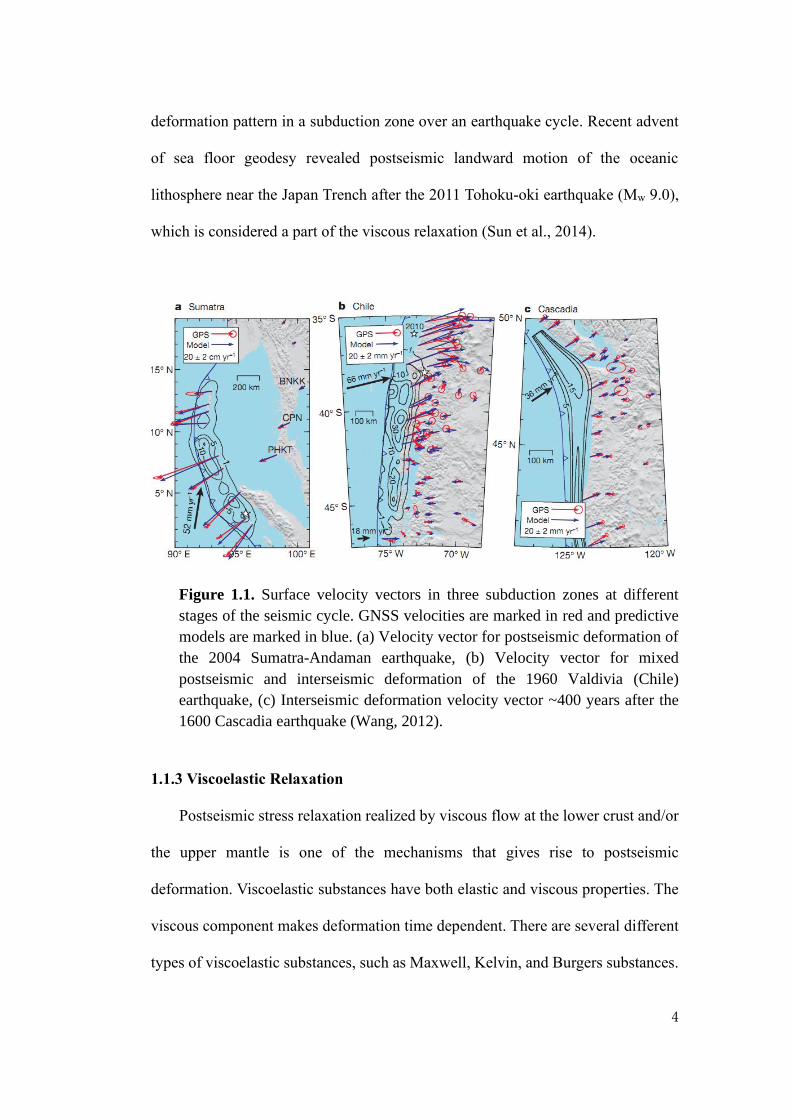
deformation pattern in a subduction zone over an earthquake cycle. Recent advent

of sea floor geodesy revealed postseismic landward motion of the oceanic

lithosphere near the Japan Trench after the 2011 Tohoku-oki earthquake (Mw 9.0),

which is considered a part of the viscous relaxation (Sun et al., 2014).

Figure 1.1. Surface velocity vectors in three subduction zones at different

stages of the seismic cycle. GNSS velocities are marked in red and predictive

models are marked in blue. (a) Velocity vector for postseismic deformation of

the 2004 Sumatra-Andaman earthquake, (b) Velocity vector for mixed

postseismic and interseismic deformation of the 1960 Valdivia (Chile)

earthquake, (c) Interseismic deformation velocity vector ~400 years after the

1600 Cascadia earthquake (Wang, 2012).

1.1.3 Viscoelastic Relaxation

Postseismic stress relaxation realized by viscous flow at the lower crust and/or

the upper mantle is one of the mechanisms that gives rise to postseismic

deformation. Viscoelastic substances have both elastic and viscous properties. The

viscous component makes deformation time dependent. There are several different

types of viscoelastic substances, such as Maxwell, Kelvin, and Burgers substances.

5

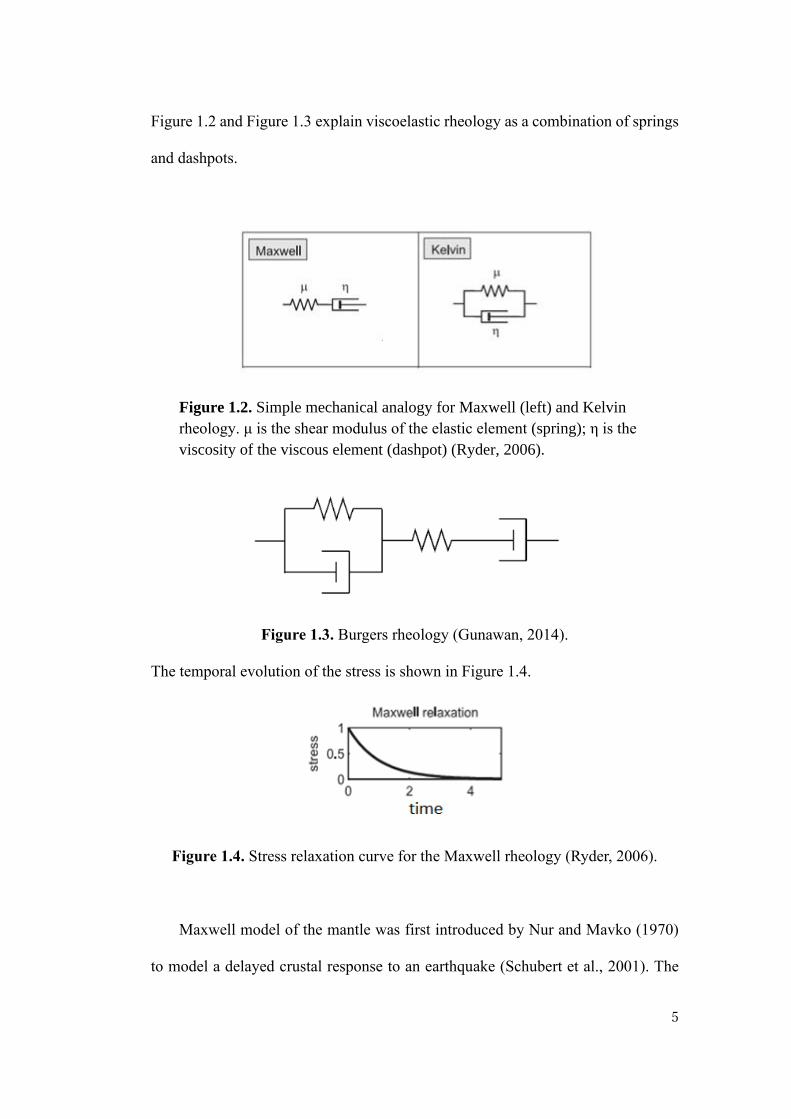
Figure 1.2 and Figure 1.3 explain viscoelastic rheology as a combination of springs

and dashpots.

Figure 1.2. Simple mechanical analogy for Maxwell (left) and Kelvin

rheology. μ is the shear modulus of the elastic element (spring); η is the

viscosity of the viscous element (dashpot) (Ryder, 2006).

Figure 1.3. Burgers rheology (Gunawan, 2014).

The temporal evolution of the stress is shown in Figure 1.4.

Figure 1.4. Stress relaxation curve for the Maxwell rheology (Ryder, 2006).

Maxwell model of the mantle was first introduced by Nur and Mavko (1970)

to model a delayed crustal response to an earthquake (Schubert et al., 2001). The

6

Maxwell's rheology has been shown to fit various kinds of deformation in

subduction zones such as Chile (Moreno et al., 2011; Wang, 2007) and Alaska

(Suito and Freymueller, 2009). Pollitz et al. (2006) showed that the Burgers

rheology gave better fit to model co- and postseismic crustal deformation of the

2004 Sumatra-Andaman earthquake than the Maxwell model.

1.2 A Brand-New Process in the Earthquake Cycle

Heki and Mitsui (2013) reported unexpected increase of the landward

movements of forearc GNSS stations in segments adjacent along-strike to the

megathrust rupture after the 2003 Tokachi-oki earthquake (Mw 8.3), and possibly

after the 2011 Tohoku-oki earthquake (Figure 1.5).

Figure 1.5. The locations of the earthquakes studied here. Red circles represent

the six earthquakes that showed postseismic increased landward velocity in

segments adjacent to megathrust ruptures. Numbers attached to the earthquakes

correspond to those in Table 1. Gray circles represent megathrust earthquakes

that may have caused such velocity changes, but I failed to find enough GNSS

data from stations in appropriate places with enough time span for pre- and

postseismic periods (Section 5.1).

7

General features of this phenomenon are illustrated in Figure 1.6. After

earthquakes, GNSS stations near the ruptured fault would move trenchward due to

afterslip and viscous relaxation (Figure 1.6b). In addition to it, Heki and Mitsui

(2013) found that stations on segments adjacent to the ruptured fault showed

landward increase of movements as illustrated with green arrows in Figure 1.6b.

This looks as if interplate coupling in the neighboring segments of the rupture has

increased.

Figure 1.6. Schematic illustration of interseismic movements of GNSS stations

(a) and their changes by a large earthquake (b). The trenchward movements in

(b) occur driven by afterslip and postseismic relaxation around the ruptured

fault. In addition to this, interseismic landward velocities often increase in

segments adjacent along-trench to the ruptured segment (station X).

This phenomenon cannot be explained by classical viscoelastic relaxation.

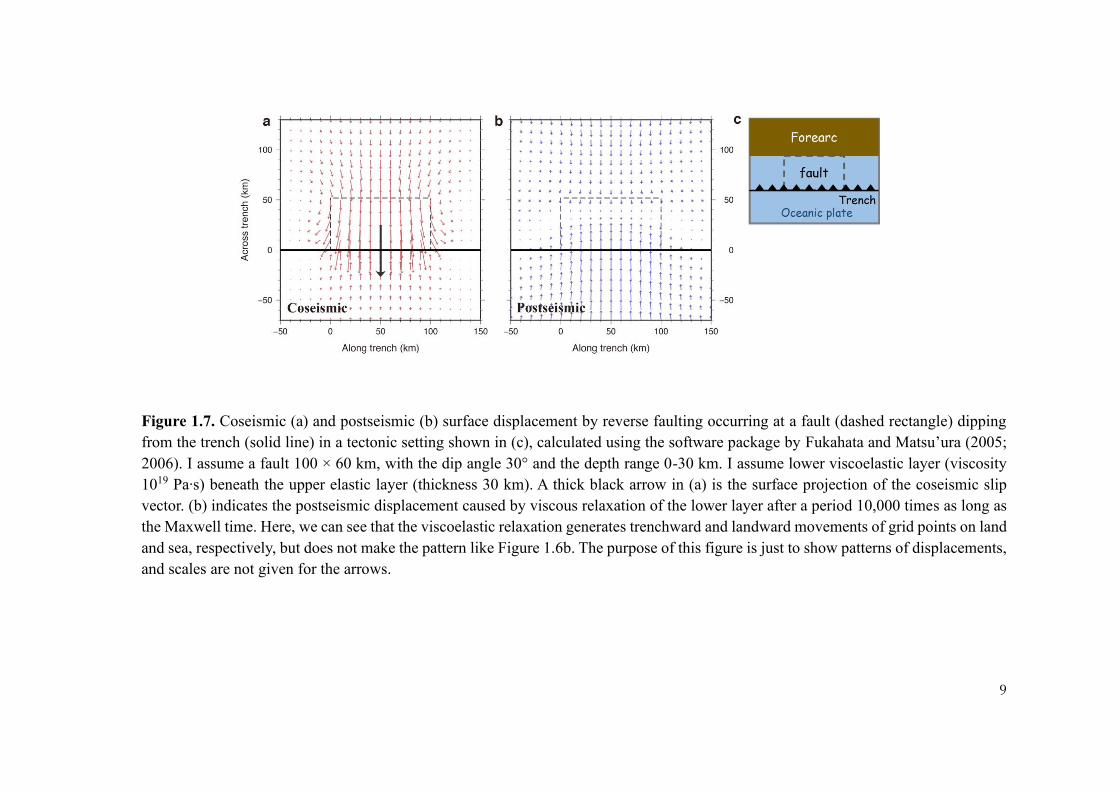
Figure 1.7 shows coseismic jump and slow movements caused by postseismic

viscous relaxation calculated for a simple thrust earthquake case following

Fukahata and Matsu’ura (2005; 2006). Postseismic deformation continues as the

shear stress within viscous asthenosphere decays and let the deformation pattern

reach the final state realizing the two-dimensional mechanical equilibrium within

8

the lithosphere.

Figure 1.7b demonstrates that postseismic viscoelastic relaxation generates

only trenchward movement of forearc GNSS stations. In other words, landward

increase of velocity as seen for station X in Figure 1.6 does not occur in the adjacent

segments. This situation remains similar even with different settings of parameters,

e.g. elastic thickness, viscosity of underlying asthenosphere, geometry of the fault.

So, the postseismic acceleration of landward velocities as shown in Figure 1.6b

would need an explanation with some other mechanisms.

9

Figure 1.7. Coseismic (a) and postseismic (b) surface displacement by reverse faulting occurring at a fault (dashed rectangle) dipping

from the trench (solid line) in a tectonic setting shown in (c), calculated using the software package by Fukahata and Matsu’ura (2005;

2006). I assume a fault 100 × 60 km, with the dip angle 30° and the depth range 0-30 km. I assume lower viscoelastic layer (viscosity

1019 Pa∙s) beneath the upper elastic layer (thickness 30 km). A thick black arrow in (a) is the surface projection of the coseismic slip

vector. (b) indicates the postseismic displacement caused by viscous relaxation of the lower layer after a period 10,000 times as long as

the Maxwell time. Here, we can see that the viscoelastic relaxation generates trenchward and landward movements of grid points on land

and sea, respectively, but does not make the pattern like Figure 1.6b. The purpose of this figure is just to show patterns of displacements,

and scales are not given for the arrows.

10

Mavrommatis et al. (2014) suggested that the increased coupling in the

northernmost Honshu after the 2003 Tokachi-oki earthquake (Segment 3 in Figure

1b of Heki and Mitsui, 2013) reflects the termination of the afterslip of the 1994

Mw 7.6 Sanriku-oki earthquake (Heki et al., 1997). This, however, does not explain

the landward velocity increase seen at the neighboring segment on the other side

(Segment 1 in Figure 1b of Heki and Mitsui, 2013) of the 2003 Tokachi-oki rupture.

Small-scale change of interplate coupling can be explained by the pore fluid

pressure changes associated with coseismic fluid migration along the plate interface

(Materna et.al., 2019). However, large-scale enhanced coupling that may occur in

the adjacent segments cannot be explained by that mechanism.

1.3 Previous works

To explain the postseismic increase of landward velocity in adjacent segments,

Heki and Mitsui (2013) hypothesized that the coseismic stress drop modified the

force balance acting on the subducting slab around the ruptured segment and

induced accelerated subduction of the oceanic plate, a concept similar to the

classical idea of Anderson (1975) (Figure 1.4). Uchida et al. (2016) found

accelerated interplate creep rates from slip accumulation rates of small repeating

earthquakes beneath the Kanto area following the 2011 Tohoku-oki earthquake,

which serves as a seismological evidence of the accelerated subduction. Outside

NE Japan, Melnick et al. (2017) found the increased landward velocity in central

Chile, at GNSS stations located to the north of the 2010 Maule earthquake (Mw 8.8)

rupture. Melnick et al. (2017) called it super-interseismic period that occur at the

early stage of an earthquake cycle, and Loveless (2017) considered it a common

11

phenomenon after megathrust earthquakes (Figure 1.9).

Figure 1.8. Accelerated subduction and enhanced earthquake activity proposed

by Anderson (1975). When the decoupling earthquake occurs at time t1, the

stresses of the lithosphere in the segment of t1 decrease and accelerated

subduction starts. This causes the stresses at the segments of t2 and t3 of the arc

boundary to increase, leading to subsequent earthquakes at times t2 and t3.

Melnick et al. (2017) suggested that this enhanced landward velocity might

have triggered the 2015 Illapel earthquake (Mw 8.3) and the 2016 Chiloé earthquake

(Mw 7.6) that occurred to the north and south of the Maule rupture, respectively.

Heki and Mitsui (2013) considered the accelerated slab subduction may explain

temporary increase of regional seismicity such as the sequences of megathrust

earthquakes in 1950s-1960s in Kamchatka-Aleutian subduction zones (Kanamori,

1978). Indeed, in the Kuril-NE Japan subduction zone, the 2003 Tokachi-oki, the

2004 Kushiro-oki (Mw 7.0), the 2006 central Kuril (Mw 8.3), and the 2011 Tohoku-

oki earthquakes occurred within 8 years. Considering the large along-trench extent

of these earthquakes, it would be difficult to explain it just by static stress

perturbations (King et al., 1994).

12

Figure 1.9. Schematic model of postseismic velocity changes according to

Loveless (2017). Rotation of the upper plate increases landward velocity

adjacent to the rupture zone, consistent with enhanced coupling on the interface

beneath these regions. The enhanced coupling may be the site of subsequent

earthquakes encouraged by the “super-interseismic” coupling.

The scope of the present study is to explore similar examples worldwide, taking

advantage of the rapid expansion of GNSS networks in various subduction zones,

using station coordinate data covering periods before and after megathrust

earthquakes. I then try to find common features and discuss if the compiled data

support a certain model, e.g. the slab acceleration model by Heki and Mitsui (2013).

1.4 Objectives

The purpose of this study is to use the GNSS (Global Navigation Satellite

System) measurements to investigate crustal deformation, particularly related to

landward increase of surface velocity following six megathrust earthquakes in four

subduction zones, including NE Japan, central and northern Chile, Sumatra, and

Mexico. I collect as much geodetic information as possible to facilitate the

discussion on the model responsible for the postseismic landward change in

velocities. I also try to detect increases in seismicity in the segment showing

enhanced coupling after the 2011 Tohoku-oki and the 2010 Maule earthquakes.

13

However, I do not aim at proving particular models including the slab acceleration

model by Heki and Mitsui (2013).

1.5 Dissertation outline

This dissertation consists of several Chapters. The brief explanations of the chapters

are given below:

Chapter 1 explains the background of this research and the objectives of the

research. The last sub-chapter gives the explanation of the outline of this

dissertation.

Chapter 2 describes GNSS data in general, those used in individual cases, and time

series analysis strategies. Time series analyses are important because the studied

cases have different quality and quantity of GNSS data sets. This chapter also

describes the method I employed. The first step of the method is to rotate the two

horizontal axes (north and east) so that the two components coincide with the

direction parallel with or perpendicular to the station's interseismic movement

before the earthquakes. Then, trench-normal landward velocity changes are

discussed. In this chapter, I also review the slab acceleration model by Heki and

Mitsui (2013). Even though the purpose of this study is not to prove the model, their

model is important for the exploration of physical mechanisms responsible for the

postseismic landward change in velocities.

14

Chapter 3 describes the landward velocity change that occurred in Japan, Chile,

Sumatra-Indonesia, and Mexico. I use the method shown in chapter 4 and give brief

description of the tectonic setting of the studied subduction zones. A typical analysis

starts with mapping the postseismic crustal movements of the studied earthquake,

where one can see distributions of landward and trenchward velocity changes

following the earthquake. The stations showing landward velocity changes are

selected for further analysis. There, the distances of stations from the fault are

considered as an important factor. To present the analysis results, I show the maps

and diagrams that show the differences in the velocities following the earthquake

relative to the reference velocities before the earthquake.

Chapter 4 contains the overview of the six earthquake cases discussed in the

previous chapter. Furthermore, I also discuss the spatial extent of the enhanced

coupling, which is closely related to the hypothesis that the enhanced coupling may

encourage future failures in the neighboring segments. The next sub-chapter

describes the relationship between forearc station velocities and slab velocities. I

convert the landward velocity change observed at each station (v'-v) to hypothetical

slab acceleration (u'-u). At the end of this chapter, I compare the properties of data

with those predicted by the slab acceleration model (Heki and Mitsui, 2013).

15

In Chapter 5, I discuss the change in seismicity following the earthquakes. I expect

that the increase of landward velocity is correlated positively with the background

seismicity. To make the analysis more robust, I removed clustered earthquakes such

as swarms and aftershocks from the earthquake catalog using a stochastic de-

clustering method developed by Ogata (1988).

In Chapter 6, I summarize the findings related to the interplate coupling

enhancement in adjacent segments following megathrust ruptures.

16

Chapter 2: Data and Method

2.1 GNSS Data

I analyzed Global Navigation Satellite System (GNSS) data in forearc regions

of subduction zones such as the western Sumatra, Northeast Japan, central and

northern Chile, and in the Oaxaca region, Mexico.

GNSS is the system that covers the whole earth. The first GNSS is the American

system called Global Positioning System (GPS) started full operation in 1990s.

Later, three new GNSS have been added, e.g. Russian GNSS called Global

Navigation Satellite System (GLONASS), European GNSS called Galileo, Chinese

system called Compass/Beidou. There are smaller systems designed as regional

satellite positioning systems. They include the Indian Regional Navigation Satellite

System (IRNSS), and the Japanese Quasi-Zenith Satellite System (QZSS).

GPS, formally called NAVSTAR GPS (Navigation Satellite Timing and Ranging

Global Positioning System), was developed by the Department of Defense of USA

in late 1970s and 1980s initially for military purposes. However, it has become a

indispensable tool as a versatile geodetic tool for studying various geophysical

phenomenon. Over the last three decades, GPS has made a significant impact on a

wide range of geophysical disciplines.

By using GPS, Larsen et al. (1992) detected coseismic crustal deformation of the

1987 Superstition Hills earthquake (Mw 6.2), and Lisowski et al. (1990) studied the

coseismic deformation of the 1989 Loma Prieta, California, earthquake (Mw 7.1).

17

These two investigations were among the early utilization of GNSS to understand

crustal deformation associated with earthquakes. Then, GNSS can be utilized to

understand postseismic deformation behavior as more data recorded year by year.

The 1989 Loma Prieta earthquake (Mw 7.1) and the 1992 Landers earthquake (Mw

7.3) were the examples of the first earthquake events whose postseismic signal was

well recorded (Savage et al., 1994; Bürgmann et al., 1997; Shen et al., 1994; Savage

and Svarc, 1997). The first dense array of GNSS was established in Japan during

1990s. This array first detected coseismic deformation of the 1994 Hokkaido-Toho-

Oki earthquake (Tsuji et al., 1995) and postseismic deformation of the 1994

Sanriku-Haruka-Oki earthquake (Mw 7.5) (Heki et al., 1997). After that, they

studied crustal deformation related to many earthquakes with magnitudes exceeding

6 in and around Japan (Sagiya, 2004).

The recent advance of space geodetic technology revealed new kinds of crustal

deformation related to earthquakes. Sato et al. (2011) detected coseismic sea floor

movement associated with the 2011 Tohoku-oki earthquake (Mw 9.0). This was

followed by Sun et al. (2014), which revealed the postseismic landward motion of

the oceanic lithosphere near the Japan Trench. Heki and Mitsui (2013) found a

increase of the landward movements of GNSS stations in segments adjacent along-

strike to the megathrust rupture, the 2003 Tokachi-oki earthquake (Mw 8.3) and the

2011 Tohoku-oki earthquake.

Below I give brief descriptions of the GNSS data used in this study. Nowadays,

the movements of GNSS stations are described within the International Terrestrial

Reference Frame (ITRF). These velocities align with the no-net-rotation plate

motion models and were converted to those relative to the landward plate by

subtracting velocities calculated using the nnr-MORVEL56 model (Argus et al.,

18

2011). Because I discuss changes in velocity before and after large earthquakes,

common bias to these velocities is canceled. This means that results in the present

study are not so sensitive to the selection of the plate motion model.

2.1.1 GNSS Data in Japan

In Japan, we used the F3 solution of the dense continuous GNSS array called

GNSS Earth Observation Network System (GEONET). This network is composed

of more than 1,300 stations with an average separation of ~20 km and covers the

whole Japanese archipelago (Figure 2.1). It is operated by the Geospatial

Information Authority (formerly Geographical Survey Institute) (GSI), Japan, and

the data are made open to worldwide geodetic communities. The F3 solution is

obtained by using the Bernese software fixing a certain station in Tsukuba, near the

GSI headquarter, to the coordinates determined daily using stations in the Asia

Pacific region (Nakagawa et al., 2009).

For the 2003 earthquake, I followed the procedure by Heki and Mitsui (2013)

and fixed the Kamitsushima station, north of Kyushu, and compared the velocity

difference before and after the earthquake. For the 2011 earthquake, the

Kamitsushima station, ~1,000 km away from the epicenter, exhibited a few mm/yr

postseismic movements. Hence, I did not fix any stations and subtracted the

movement of the landward plate calculated with the nnr-MORVEL56 plate motion

model (Argus et al., 2011) from the coordinate changes in the F3 solution expressed

in ITRF.

19

Figure 2.1. Distribution of GEONET stations (https://www.un-ggim-ap.org/

meetings/ pm/5th/201607/W020161027635538377589.pdf)

2.1.2 GNSS Data in Sumatra

In Sumatra, there are several GNSS network systems operated by different

institutions. The Geospatial Agency of Indonesia (BIG) initiated geodetic networks

for geodynamics studies in Sumatra in 1989 (Abidin et al., 2016). A total of 60

GNSS stations on Sumatra and surrounding islands, installed in 1989, 1991, and

1993, were used to detect crustal movements in the Sumatran subduction zone

(Prawirodirjo et al., 1997). In 2002, Caltech (California Institute of Technology)

20

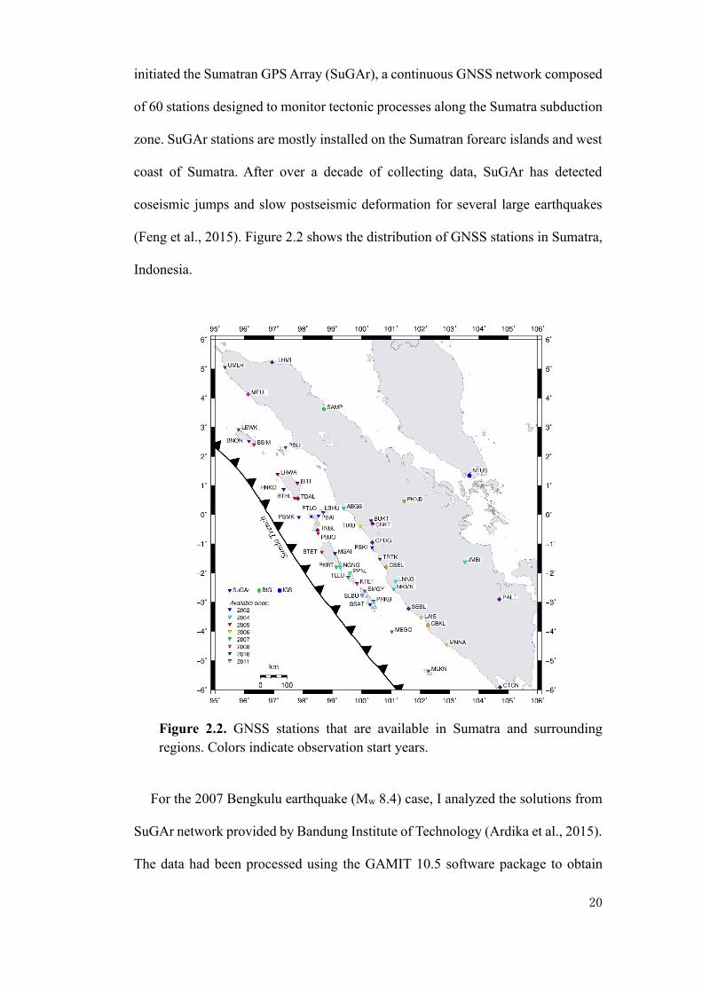
initiated the Sumatran GPS Array (SuGAr), a continuous GNSS network composed

of 60 stations designed to monitor tectonic processes along the Sumatra subduction

zone. SuGAr stations are mostly installed on the Sumatran forearc islands and west

coast of Sumatra. After over a decade of collecting data, SuGAr has detected

coseismic jumps and slow postseismic deformation for several large earthquakes

(Feng et al., 2015). Figure 2.2 shows the distribution of GNSS stations in Sumatra,

Indonesia.

Figure 2.2. GNSS stations that are available in Sumatra and surrounding

regions. Colors indicate observation start years.

For the 2007 Bengkulu earthquake (Mw 8.4) case, I analyzed the solutions from

SuGAr network provided by Bandung Institute of Technology (Ardika et al., 2015).

The data had been processed using the GAMIT 10.5 software package to obtain

21

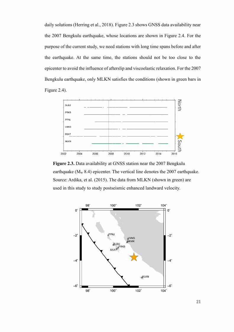
daily solutions (Herring et al., 2018). Figure 2.3 shows GNSS data availability near

the 2007 Bengkulu earthquake, whose locations are shown in Figure 2.4. For the

purpose of the current study, we need stations with long time spans before and after

the earthquake. At the same time, the stations should not be too close to the

epicenter to avoid the influence of afterslip and viscoelastic relaxation. For the 2007

Bengkulu earthquake, only MLKN satisfies the conditions (shown in green bars in

Figure 2.4).

Figure 2.3. Data availability at GNSS station near the 2007 Bengkulu

earthquake (Mw 8.4) epicenter. The vertical line denotes the 2007 earthquake.

Source: Ardika, et al. (2015). The data from MLKN (shown in green) are

used in this study to study postseismic enhanced landward velocity.

22

Figure 2.4. Location of GNSS stations near the 2007 Bengkulu earthquake

(Mw 8.4) epicenter. Star indicates the location of largest coseismic slip of the

earthquake.

2.1.3 GNSS Data in South and Middle America

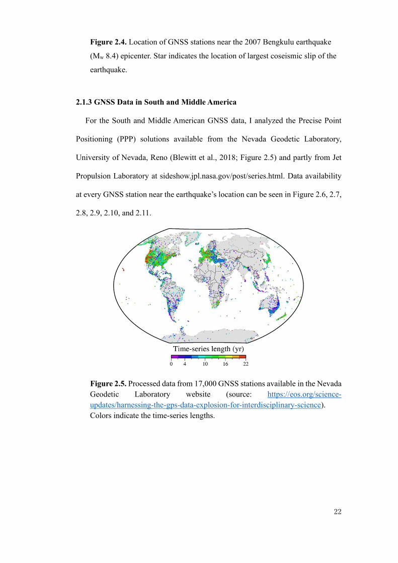
For the South and Middle American GNSS data, I analyzed the Precise Point

Positioning (PPP) solutions available from the Nevada Geodetic Laboratory,

University of Nevada, Reno (Blewitt et al., 2018; Figure 2.5) and partly from Jet

Propulsion Laboratory at sideshow.jpl.nasa.gov/post/series.html. Data availability

at every GNSS station near the earthquake’s location can be seen in Figure 2.6, 2.7,

2.8, 2.9, 2.10, and 2.11.

Figure 2.5. Processed data from 17,000 GNSS stations available in the Nevada

Geodetic Laboratory website (source: https://eos.org/science-

updates/harnessing-the-gps-data-explosion-for-interdisciplinary-science).

Colors indicate the time-series lengths.

23

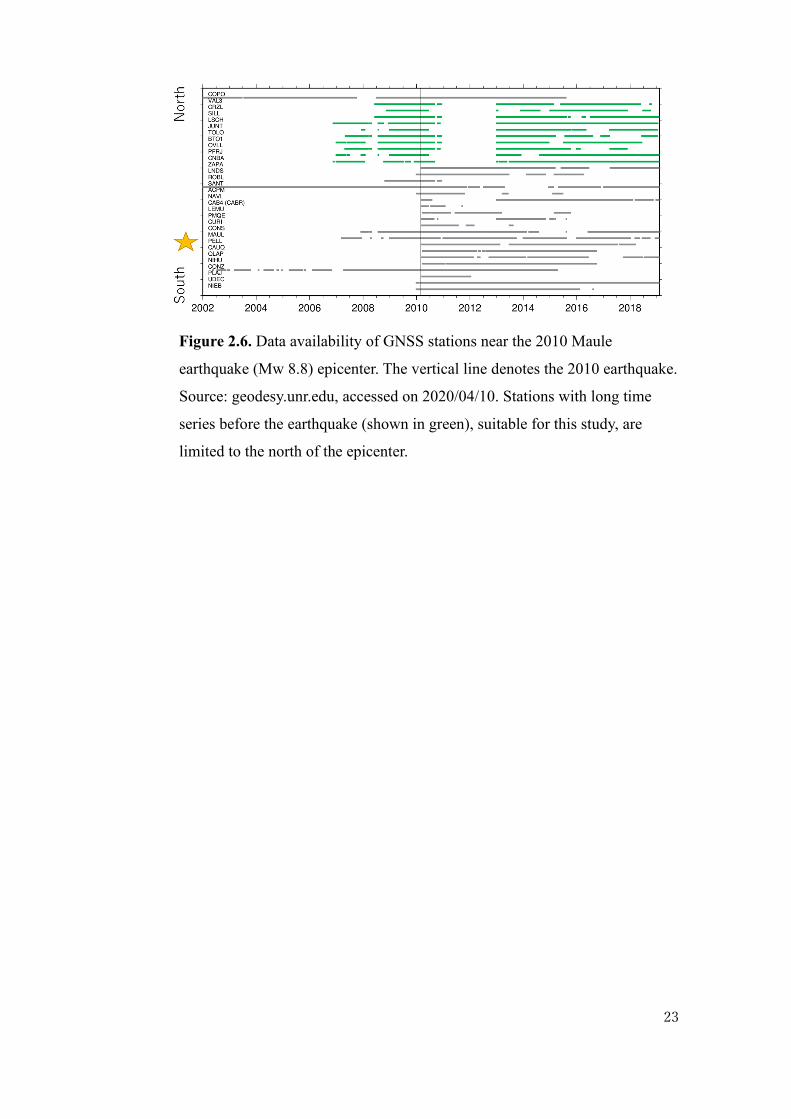
Figure 2.6. Data availability of GNSS stations near the 2010 Maule

earthquake (Mw 8.8) epicenter. The vertical line denotes the 2010 earthquake.

Source: geodesy.unr.edu, accessed on 2020/04/10. Stations with long time

series before the earthquake (shown in green), suitable for this study, are

limited to the north of the epicenter.

24

Figure 2.7. Location of GNSS stations near the 2010 Maule earthquake (Mw

8.8) epicenter shown in Figure 2.6. Star indicates the location of largest

coseismic slip of this earthquake.

25

Figure 2.8. Data availability of GNSS stations in northern Chile and Peru for

the study of the 2014 Iquique earthquake. The vertical line denotes the 2014

earthquake. Source: geodesy.unr.edu and sideshow.jpl.nasa.gov/post/series

(for AREQ station). Accessed on 2020/04/10.

Figure 2.9. Location of GNSS stations near the 2014 Iquique earthquake (Mw

8.2) epicenter shown in Figure 2.8. Star indicates the location of largest

coseismic slip of the earthquake.

26

Figure 2.10. Data availability at GNSS station near the 2012 Oaxaca

earthquake (Mw 7.4) epicenter. The vertical line denotes the 2012 earthquake.

Only one station (OXPE, shown in green) was suitable for the purpose of this

study. Source: geodesy.unr.edu. Accessed on 2020/04/10.

Figure 2.11. Location of GNSS stations near the 2012 Oaxaca earthquake

(Mw 7.4) epicenter. Star indicates the location of largest coseismic slip of the

earthquake.

2.1.4 Time series analysis strategy

The target of this study is the “landward” velocity changes in the forearc region

27

of the segment adjacent along-trench to the megathrust ruptures. Therefore, I have

to avoid GNSS stations suffering from postseismic “trenchward” movements. They

are caused by well-known mechanisms such as afterslip and viscous relaxation of

asthenosphere. Such movements have already been well documented in literatures

for individual earthquakes, such as Yamagiwa et al. (2015) for the 2011 Tohoku-oki

earthquake, Miyazaki et al. (2004) for the 2003 Tokachi-oki earthquake, Klein et al.

(2016) for the 2010 Maule earthquake, Hoffmann et al. (2018) for the 2014 Iquique

earthquake, and Lubis et al. (2012) for the 2007 Bengkulu earthquake.

To select stations showing landward velocity changes, I checked not only the

polarities of trench-normal velocities but also the distance of stations from the fault

edge. This is because the enhanced inter-plate coupling studied here tend to occur

in a certain range of distance, i.e. they occur in forearc from the fault edge over a

distance comparable to a half of the fault length. This will be discussed later in

Chapter 4.2.

In calculating the velocity changes of the selected GNSS stations, I compare

velocities during the two periods before and after the earthquakes (Table 1). These

periods should be long enough to enable estimation of accurate velocities (longer

than two years to robustly remove seasonal changes) and hopefully be immediately

before and after earthquakes. Actually, I often have to shift or shorten these periods

to avoid unwanted transient movements caused by other smaller earthquakes during

the studied periods.

It should be noted that landward velocity changes depend on the selection of

time windows. For example, such velocity changes are often unstable during the

first few years while postseismic transient movements continue. I will discuss this

problem comparing velocities in different time windows in Chapter 4.3.

28

I also need to pay attention to past earthquakes in nearby segments. Large

interplate earthquakes are followed by trenchward postseismic movements of

GNSS stations lasting for years. Their temporal decay might leak into the

postseismic landward velocity increases, the target of the present study. For the six

earthquakes studied here, I discuss potential influences from such past earthquakes

in Chapter 3.

29

Table 1. Two periods used to estimate velocity changes before and after the earthquakes (Figure 1).

No. Earthquake (Mw) Before earthquake After earthquake3

1 2011/3/11 Tohoku-oki (9.0) 2008.00-2011.19 2011.19-2015.00

2 2003/9/25 Tokachi-oki (8.3) 1996.00-2003.741 2003.74-2010.10

3 2010/2/28 Maule (8.8) ~2008.002-2010.16 2010.16-2014.70

4 2014/4/1 Iquique (8.2) ~2010.002-2014.25 2014.25-2019.25

5 2007/9/12 Bengkulu (8.4) 2005.50-2007.70 2007.70-2010.814

6 2012/3/20 Oaxaca (7.4) 2010.38-2012.22 2012.22-2017.22

1Shifted to 1996.0-2003.0 to avoid influence of the Miyagi-oki earthquake (Mw 7.0) on

2003 May 26 for stations close to its epicenter 2Earliest possible starting times are used depending on the availability of the stations 3The early non-linear postseismic periods avoided to draw Figures 6a, 7a, and 8a. 4Only data until the occurrence of the 2010 Mentawai earthquake are used.

30

2.2 Method for acceleration analysis

I model the time series of the two horizontal components of a GNSS station

coordinate considering linear trends, average seasonal (annual and semiannual)

changes, jumps associated with antenna replacements (for GEONET stations), and

coseismic jumps. In addition to these standard parameters, I estimate the coseismic

changes in velocity (v’-v). The velocities are expressed relative to the stable part of

the landward plates of the subduction zones (Figure 2.12). I also discuss possible

existence of non-linear movements shortly after earthquakes and their influences

later in Chapter 4.3.

Figure 2.12. Landward movement time series of the stations MLKN (Bengkulu,

Indonesia) and 0531 (Hokkaido, Japan). Both two time series are modeled

considering linear trends (including changes in trends associated with

earthquakes), jumps caused by antenna replacements (for GEONET stations),

and average seasonal changes. The average seasonal components are removed

in the upper time series.

In Chapter 3, I show a set of figures as shown in Figure 2.13, for each megathrust

earthquake. I first rotate the two horizontal axes (north and east) so that the two

components coincide with the direction parallel with (red in Figure 2.13a) or

perpendicular to (blue in Figure 2.13a) the interseismic movement of the station

before the earthquakes (normally in the direction of the subducting oceanic plate).

In the plot, I subtract the estimated average seasonal components.

31

In the diagram, the coseismic increase of the landward velocity of a GNSS station

appears as the positive change in the slope of the red time series (Figure 2.13a). The

blue (trench-parallel) component represents the change in the direction of the

movement by the earthquakes. This is expected to be small. Both components often

show coseismic jumps, but they are not the target of the present study.

Figure 2.13. An example of the analysis of the velocity change after a large

earthquake for the station X shown in Figure 1.6. (a) I rotate the horizontal axes

so that one axis coincides with the interseismic movement direction (red) and

the other axis is perpendicular to it (blue). Thus, the increase of the landward

velocity of a GNSS station can be seen as the increased slope of the red

component. In the small panel atop, I remove the pre-earthquake linear trend

(dotted line) to isolate postseismic changes in trend. Y-axis represents the

movement in the trench-normal (landward) and trench-parallel azimuths. (b)

Concept of the increased interseismic velocity which is the sum of the

interseismic velocity before the earthquake and the coseismic velocity change.

Here, I do not discuss vertical components. In fact, changes in vertical velocities

were not significant for the 2003 case as reported in Heki and Mitsui (2013). This

partly comes from intrinsic large uncertainty in determining the vertical positions.

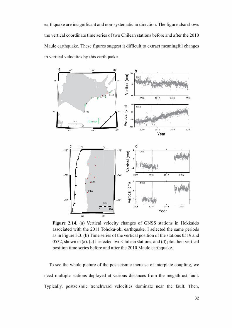
Figure 2.14 shows that vertical velocities changes following the 2011 Tohoku-oki

32

earthquake are insignificant and non-systematic in direction. The figure also shows

the vertical coordinate time series of two Chilean stations before and after the 2010

Maule earthquake. These figures suggest it difficult to extract meaningful changes

in vertical velocities by this earthquake.

Figure 2.14. (a) Vertical velocity changes of GNSS stations in Hokkaido

associated with the 2011 Tohoku-oki earthquake. I selected the same periods

as in Figure 3.3. (b) Time series of the vertical position of the stations 0519 and

0532, shown in (a). (c) I selected two Chilean stations, and (d) plot their vertical

position time series before and after the 2010 Maule earthquake.

To see the whole picture of the postseismic increase of interplate coupling, we

need multiple stations deployed at various distances from the megathrust fault.

Typically, postseismic trenchward velocities dominate near the fault. Then,

33

landward increased velocities (enhanced coupling signature) emerge as we go away

along trench from the fault (Figure 1.6b). This enhanced coupling would then decay

as we go farther away from the fault.

It is usually difficult to see them all due to the insufficient availability of GNSS

stations along the forearc. In this study, I use multiple stations to represent the

landward velocity change whenever possible. Nevertheless, I sometimes have to let

just one station represent the increase of the landward velocity for certain

earthquakes. In the discussion, I compile all the cases to extract common features

so that I can discuss the physical model behind the phenomenon.

For very large earthquakes, postseismic velocity changes can occur in a

continental scale as shown in Melnick et al. (2017) in South America following the

2010 Maule earthquake. It is also likely that a similar situation occurred following

the 2011 Tohoku-oki earthquake as seen in GNSS point velocities in China (Shao

et al., 2015). In this study, I focus on the velocity changes occurring near the

ruptured faults.

2.3 Slab acceleration model by Heki and Mitsui (2013)

The purpose of this study is to collect as much geodetic information as possible

to facilitate the discussion on the model responsible for the postseismic landward

change in velocities. I do not aim at proving a particular model, including the model

by Heki and Mitsui (2013). In fact, there are attempts to explain postseismic

landward velocity changes within the framework of viscous relaxation. For example,

Melnick et al. (2017) reports results by a three-dimensional thermomechanical

model to reproduce continental scale postseismic velocity changes. D’Acquisto et

al. (2020) try to explain the observed changes as the elastic bending in a horizontal

34

plane in response to the postseismic trenchward movement near the rupture area.

Other models capable of explaining the observations may also emerge in future.

Here, as one of the possibilities, I review the simple slab acceleration model Heki

and Mitsui (2013) proposed to explain the landward increased movements in

segments adjacent along-strike to a megathrust rupture.

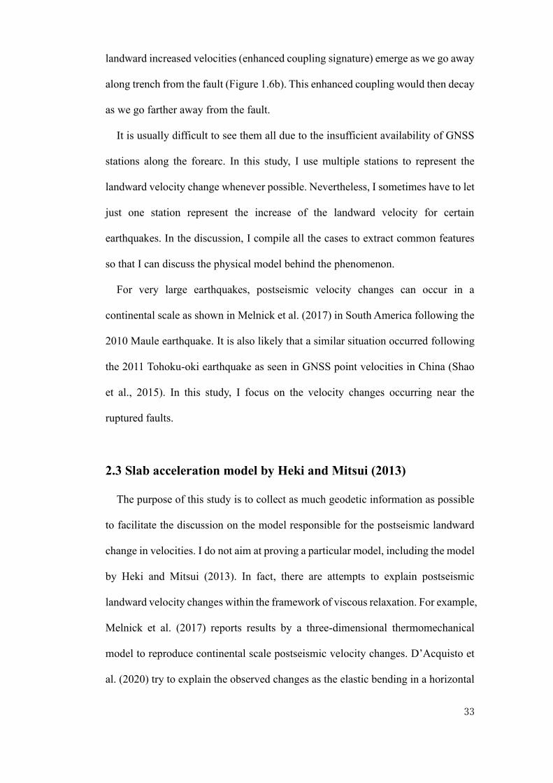
Figure 2.15a indicates the balance of forces acting on a subducting slab during

an interseismic period. There, two down-dip forces, slab pull Fsp and ridge push

Frp, are balanced with the two up-dip forces, side (partially bottom) resistance Fsr

exerted by the surrounding asthenosphere and interplate coupling Fc at the plate

interface. Fsr is proportional to the subduction speed u and I assume the resistance

occurs in a thin low-viscosity layer at the slab surface. This is a two-dimensional

model and the forces represent those working on a thin slice with a unit thickness.

Figure 2.15. Schematic view of the slab acceleration model, redrawn after Heki

and Mitsui (2013). (a) and (b) show forces acting on a subducting slab before

and after a megathrust earthquake, respectively, with a large stress drop. In (a),

downward forces (Fsp: slab pull, Frp: ridge push) are balanced by upward

forces (Fc: interplate coupling, Fsr: side resistance). In (b), sudden decrease of

the coupling Fc to Fc’ is compensated by the increase of Fsr to Fsr’ realized

by the slab acceleration from u to u’. The velocity of GNSS station before and

after the earthquake is indicated by v and v’. W is the total trench-normal length

of slab surface (both upper and lower surfaces) where viscous braking works,

and d is the thickness of the thin low viscosity layer at the lithosphere-

asthenosphere boundary.

35

Occurrence of a megathrust would reduce the coupling from Fc to Fc’, which

would be compensated by the increase of the side resistance caused by the

acceleration of the subduction speed from u to u’. Let Fc-Fc’ be the lost coupling

(stress drop integrated along-dip), and it can be related to the slab acceleration u’-u

as follows.

Fc-Fc’=Fsr’-Fsr = (u’-u) μW/d (1)

where μ is the viscosity of the low-viscosity layer with the thickness of d, and W is

the along-dip slab length (both upper and lower surface) where viscous braking

works. Then, the acceleration u’-u is expressed as

u’-u = (Fc-Fc’) d/μW (2)

For the same subduction zone with uniform μ, W and d, the acceleration u’-u would

be proportional to Fc-Fc’. Larger earthquakes would accelerate the slab more

strongly with a larger Fc-Fc’. It is actually the product of the fault width (along-dip

length) D and the stress drop .

Fc – Fc’ = D (3)

Using the average slip sav, can be expressed using the rigidity as

= sav/D. (4)

36

For the same subduction zone, I assume is the same. Then equations (3) and (4)

suggest that Fc-Fc’, and hence u’ – u, scales with the average slip sav, i.e.,

u’ – u = (d μW) sav. (5a)

In the present study, I compare cases in different subduction zones. It is generally

difficult to infer diversity of parameters , d, and for different subduction zones.

However, we can know W from seismological studies. In other words, by assuming

that d/ is the same, it may become possible to examine if the observed slab

acceleration u’-u is proportional to sav/W,

u’ – u = ( d/) sav /W. (5b)

In Chapter 4.5, I examine if the observed velocity changes for different megathrust

earthquakes in various subduction zones obey equations (5a) and (5b).

2.4 Subduction zones and slab data interpretation

According to the classical continental drift concept, the earth's surface consists

of several fragments of the continent that move relatively to each other over a

geologic timescale. The establishment of plate tectonic theory evolved from this

fundamental concept. Then, we came to recognize the mantle convection and the

formation of oceanic lithosphere along mid-oceanic ridges due to seafloor

spreading. According to the plate tectonic theory, oceanic lithosphere continuously

37

subducts into depth along convergent plate boundaries.

Subduction is the descend of a cold oceanic plate beneath a continental plate.

The slab of the oceanic lithosphere sinking into the asthenosphere provides most of

the force required to move the plates and cause the ocean floor spreading along

mid-oceanic ridges. Subduction is also responsible for bringing the surface material

such as oceanic crust, deep-sea sediments, and seawater into the depth, and their

interaction with surrounding mantle causes magma generation, arc volcanism, and

formation of continental crust.

The lengths of the subducting slabs beneath continental plates often reach

several hundreds of kilometers from the trench. Subduction zones are composed of

island arcs and deep-sea trenches and act as convergent plate boundaries. There are

two distinct subduction behaviors based on the age and type of subducting

lithosphere (Uyeda, 1982). Subduction zones with relatively steep dip angles of the

subduction are usually associated with the subduction of older oceanic lithosphere

(the Mariana type). Conversely, relatively shallow angles tend to occur where

younger oceanic plates subduct (the Chilean type). This difference controls the

seismic coupling in subduction zones. The subduction zones with denser and older

lithosphere tend to show weaker seismic coupling. On the other side, stronger

seismic coupling often occurs where young oceanic lithosphere subducts. Very

large interplate earthquakes are more common in the second type of subduction

zones.

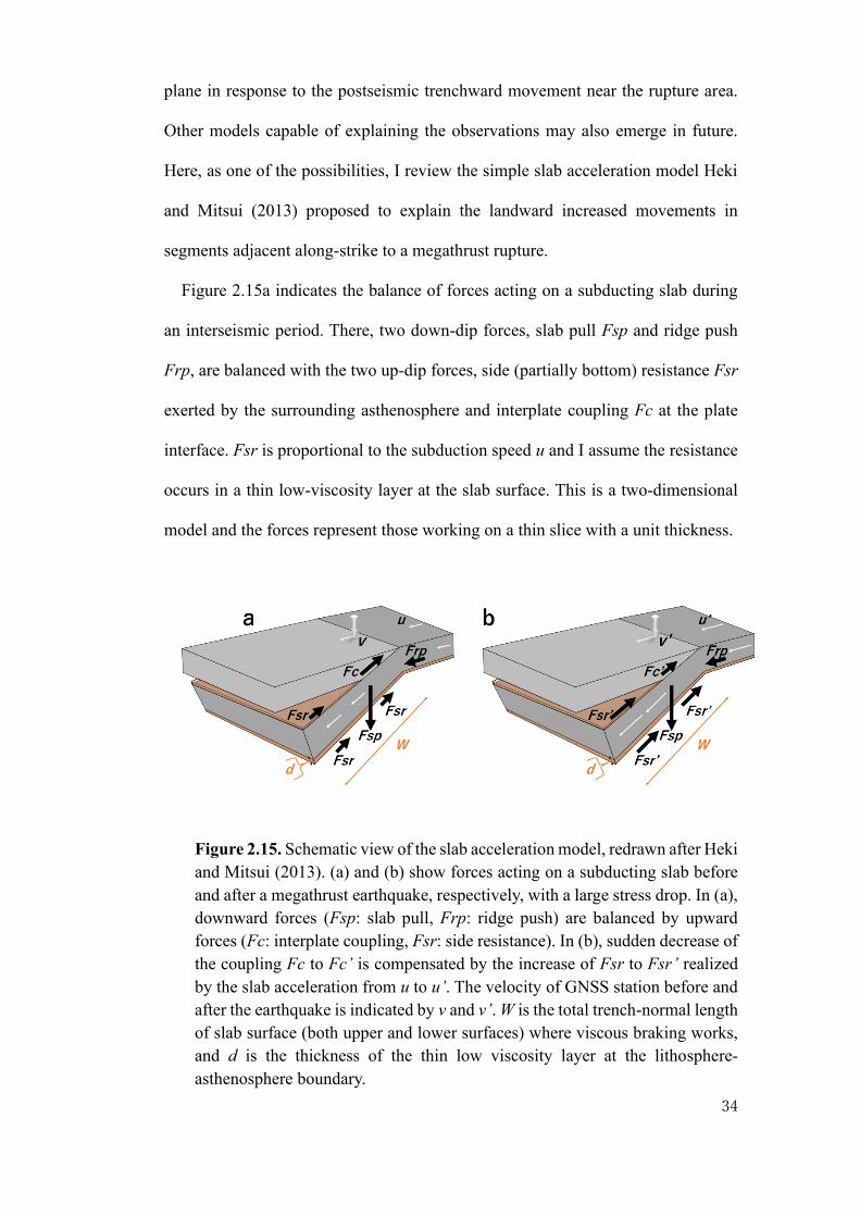
The difference of strain regime in the magmatic arc also reflects the type of

subduction zones. The steeper dip of the older lithosphere slab allows the flow of

the asthenosphere in the mantle wedge. Consequently, back-arc extensions with

38

rifting or even seafloor spreading are often found in the Mariana type subduction

zones. In contrast, compression with folding and thrusting behind the arc is

common in the Chilean type subduction zones. Such compression stems from the

frictional resistance by the subduction of young buoyant lithosphere. The difference

of the age is largely responsible for the classification into the Mariana type (>100

million-year-old) and the Chilean type (<50 million-year-old) subduction zones

(Figure 2.17).

Figure 2.17. Two different types of subduction zones (Uyeda and Kanamori

1979).

Large shallow thrust earthquakes are generated along subduction zones with

strong inter-plate locking at the plate interface. The faulting of these earthquakes

39

occur in a certain depth range called the seismogenic zone. The area of this zone

covers 2-5% of the total down-dip length of the Wadati-Benioff Zone. Actual depths

of such seismogenic zones are inferred from the rupture areas of interplate

earthquakes. In some cases, adjacent segments rupture shortly after a large

interplate earthquake. However, mechanisms governing such induced ruptures are

not fully understood. The acceleration of the slab subduction, explained in the

previous section, would be a candidate mechanism for this phenomenon.

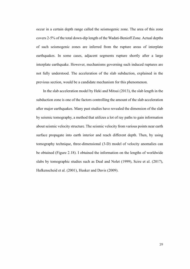
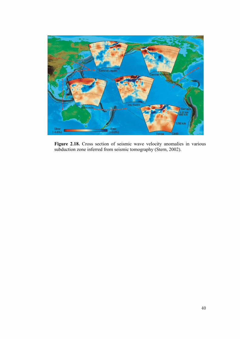
In the slab acceleration model by Heki and Mitsui (2013), the slab length in the

subduction zone is one of the factors controlling the amount of the slab acceleration

after major earthquakes. Many past studies have revealed the dimension of the slab

by seismic tomography, a method that utilizes a lot of ray paths to gain information

about seismic velocity structure. The seismic velocity from various points near earth

surface propagate into earth interior and reach different depth. Then, by using

tomography technique, three-dimensional (3-D) model of velocity anomalies can

be obtained (Figure 2.18). I obtained the information on the lengths of worldwide

slabs by tomographic studies such as Deal and Nolet (1999), Scire et al. (2017),

Hafkenscheid et al. (2001), Husker and Davis (2009).

40

Figure 2.18. Cross section of seismic wave velocity anomalies in various

subduction zone inferred from seismic tomography (Stern, 2002).

41

Chapter 3: Enhanced interplate coupling after various

megathrust earthquakes

3.1 The cases in Japan

3.1.1 Tectonic setting in Northeast Japan

The Pacific Plate is a major oceanic plate, covering some of the oldest sections

of the oceanic lithosphere. It is also one of the plates that meet, in the Japanese

Islands, with other plates such as North American (or Okhotsk), Philippine Sea, and

the Eurasian (or Amurian) Plate. The interactions among these tectonic plates cause

complicated tectonic evolution, seismicity, volcanism, and crustal deformation in

the Japanese Islands, composed of multiple island arcs such as NE Japan Arc SW

Japan Arc in the center, Ryukyu Arc to the southwest, Izu-Ogasawara Arc to the

south, and the Kuril Arc to the northeast.

The Pacific Plate subducts along the Kuril and Japan Trenches beneath the

Okhotsk Plate at a velocity of ~90 mm/yr. The definition of the Okhotsk Plate

depends of researchers. Some authors claim existences of microplates along the

boundary between the two major plates, the Eurasian and the North American Plates,

and these include the Amur and Okhotsk microplates in regions originally

considered as parts of the Eurasian and North American Plates, respectively. The

Japan Trench has a radius of about 400 km with concave-shaped westward in the

southern part, whereas, in the northern part, it is convex-shaped eastward (Niitsuma,

42

2004). The coast, backbone ranges, intermountain basins, volcanoes, and seismicity

run in parallel with the trench axes. The oceanic crust in this region was formed at

ca. 125-140 Ma and covered by pelagic sediments 1.6 km thick with a thick and

accretionary prism along the Japan trench (Kodaira et al., 2017). Several seamounts

and fracture zone were found in the oceanic crust in the northwestern Pacific Plate

(Choe and Dyment, 2020). A tomography study by Deal and Nolet (1999) suggests

that the length of the subducting slab of the Pacific Plate beneath the Okhotsk Plate

is ~1075 km. In the slab length interpretation above, I exclude the stagnant slab of

the Pacific Plate, which is deflected and flattened underneath the eastern China

(Fukao et al., 2009).

3.1.2 The 2011 Tohoku-oki earthquake (Mw 9.0)

The 2011 Tohoku-oki earthquake occurred off the Pacific coast of the Northeast

Honshu (Tohoku District), Japan. It was caused by shallow thrust faulting at the

plate boundary between the Pacific Plate and the Okhotsk (North American) Plate.

The Pacific Plate moves west-northwestward relative to the Okhotsk Plate with a

velocity of ~91 mm/year (Argus et al., 2011) and subducts underneath the NE Japan

arc at the Japan Trench. During the one hundred years period prior to the 2011

Tohoku-oki earthquake, fourteen Mw7 class earthquakes and two Mw8 class

interplate earthquakes occurred along this plate boundary (Tajima et al., 2013).

Shortly after the 2011 earthquake, the tsunami alert was issued by the Japan

Meteorological Agency (JMA) along the Pacific coast of Honshu and Hokkaido

with the prediction of maximum potential tsunami run-up height was 6 m. However,

the actual tsunami run-up height was up to 40 m, wiped out the coastal towns, and

43

inundated deeper to the inland area (Ritsema et al., 2012; Takano, 2011).

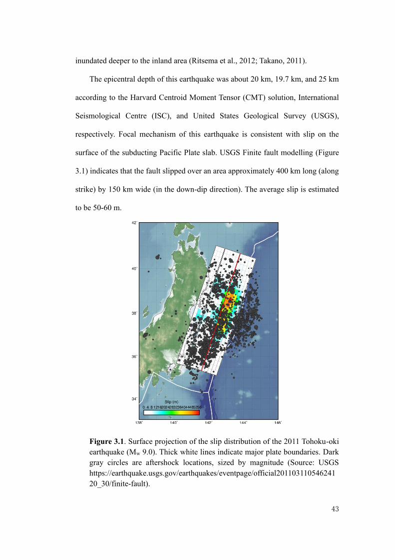
The epicentral depth of this earthquake was about 20 km, 19.7 km, and 25 km

according to the Harvard Centroid Moment Tensor (CMT) solution, International

Seismological Centre (ISC), and United States Geological Survey (USGS),

respectively. Focal mechanism of this earthquake is consistent with slip on the

surface of the subducting Pacific Plate slab. USGS Finite fault modelling (Figure

3.1) indicates that the fault slipped over an area approximately 400 km long (along

strike) by 150 km wide (in the down-dip direction). The average slip is estimated

to be 50-60 m.

Figure 3.1. Surface projection of the slip distribution of the 2011 Tohoku-oki

earthquake (Mw 9.0). Thick white lines indicate major plate boundaries. Dark

gray circles are aftershock locations, sized by magnitude (Source: USGS

https://earthquake.usgs.gov/earthquakes/eventpage/official201103110546241

20_30/finite-fault).

44

This earthquake was accompanied by a foreshock sequence lasting for ~2 days,

beginning with a Mw 7.3 event on March 9, at a point ~40 km to the north of the

mainshock epicenter. On the following day, additional six earthquakes greater than

Mw 6.0 occurred within 24 hours (Kiser and Ishii, 2012; Marsan and Enescu, 2012).

Within three months following the mainshock, more than one thousand aftershocks

were detected by >100 ocean-bottom seismometers (OBS) deployed off the Pacific

coast of the Tohoku District (Shinohara et al., 2012).

This earthquake generated large-scale postseismic deformation (e.g. Yamagiwa

et al., 2015). Such postseismic deformation, characterized by southeastward

velocity, seems to reach the southeastern half of Hokkaido. Beyond these regions

with trenchward postseismic movements, Heki and Mitsui (2013) showed that the

enhanced interplate coupling signatures are seen in eastern Hokkaido, the segment

to the northeast of the Tohoku-oki rupture.

45

Figure 3.2. (a) Differences of the velocities following the 2011 Tohoku-oki

earthquake (during 2012.00-2015.00) relative to the reference velocities before

the earthquake. GNSS stations with green arrows in (a) are free from the

trenchward postseismic crustal movement, caused by afterslip and viscoelastic

relaxation, and are used for further analyses. In (b) and (c), the green arrows

show interseismic landward movements of GNSS stations before and after the

2011 Tohoku-oki earthquake relative to the Okhotsk Plate (Table 1 summarizes

the periods used to estimate these velocities). The red arrow represents the

Pacific Plate movement relative to the Okhotsk Plate (Argus et al., 2011). Error

ellipses show 2σ errors. (d) shows the time series of the 0112 station, the dark

green arrow in (b), (c). See Figure 2.13 for the meaning of red (trench-normal,

N30.1W here) and blue (trench-parallel, N59.9E here) components. The top

46

panel of (d) shows the de-trended time series.

Figure 3.2a shows the difference of the velocities before and after the 2011

Tohoku-oki earthquake. There, the start time of the period to estimate postseismic

velocity is shifted to 2012.0 to avoid the strong non-linear behavior of the early part

of the postseismic time series. The movements of the stations are reasonably linear

in this period, but possible influences of non-linear movements are discussed later

in Chapter 4.3. We can see that trenchward postseismic movements prevail in the

Tohoku District and the western half of Hokkaido. The eastern Hokkaido shows, on

the other hand, the typical enhanced interplate coupling signature, i.e. the velocity

changes are northwestward. In drawing velocities in Figure 3.2, I converted the

velocity in ITRF to the frame fixed to the Okhotsk plate using the nnr-MORVEL56

model (Argus et al., 2011).

Figure 3.2b, c shows crustal movements before and after the 2011 Tohoku-oki

earthquake at six stations 0519, 0512, 0009, 0125, 0531, 0010, 0112, 0138, 0015,

and 0532 (from northeast to southwest). Because the postseismic trenchward

movements of the 2003 Tokachi-oki earthquake still continued in 2011, their

velocity vectors deviate significantly in azimuth from the subduction direction of

the Pacific Plate. Nevertheless, as seen in Figure 3.2a, the velocity changes at

2011.19 is clearly in the direction of the subduction, i.e. the pre-earthquake

landward movement of the GNSS stations has increased after the 2011 Tohoku-oki

earthquake.

In Figure 3.2d, I show the diagram similar to Figure 2.13 for the station 0112,

where the landward velocity increase of 8.8±0.1 mm/yr is seen. Such an error for

the increase represents 2. It is scaled with post-fit residuals but may underestimate

47

the real uncertainty. For the cases with data available from multiple stations, I use

the scatters of their increase to express their uncertainties for later discussions of

the model. One large difference from the typical case (Figure 2.13) is that even the

component perpendicular to the subduction direction (trench-parallel, blue

component in Figure 3.2d) has significant slopes. This component simply reflects

the continuation of the postseismic movement of the 2003 Tokachi-oki earthquake,

and these slopes do not show any change by the 2011 Tohoku-oki earthquake.

Similar time series from two additional stations are given in Figure 3.3. Change in

seismicity in the region showing enhanced landward movements are discussed in

Chapter 4.2. We also demonstrate that the postseismic movements of the 2003

Tokachi-oki earthquake are linear enough in 2008-2011 and its curvature does not

influence the postseismic velocity change of the 2011 earthquake as discussed later

in Chapter 4.3.

48

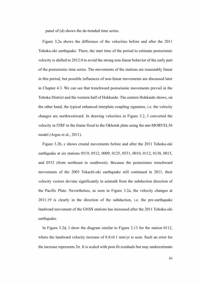
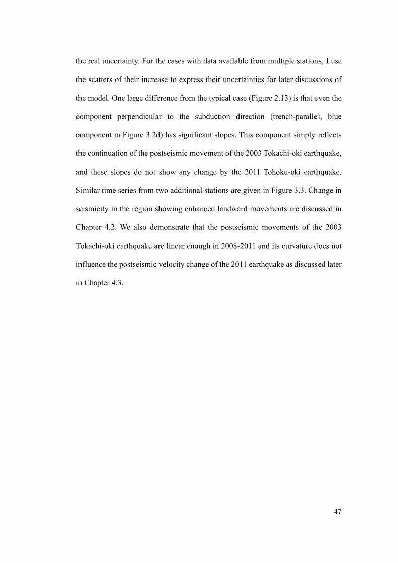
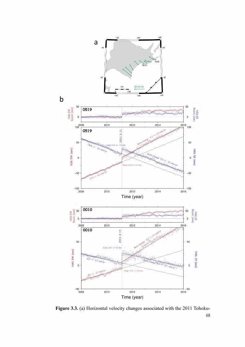
Figure 3.3. (a) Horizontal velocity changes associated with the 2011 Tohoku-

49

oki earthquake in Hokkaido (same as stations with green arrows in Figure 3.2a).

Time series of the two labeled stations (0010, 0519) are shown in (b). The

components shown in blue colors are determined as the direction perpendicular

to the velocity changes by the earthquake. The components in red are taken

perpendicular to them.

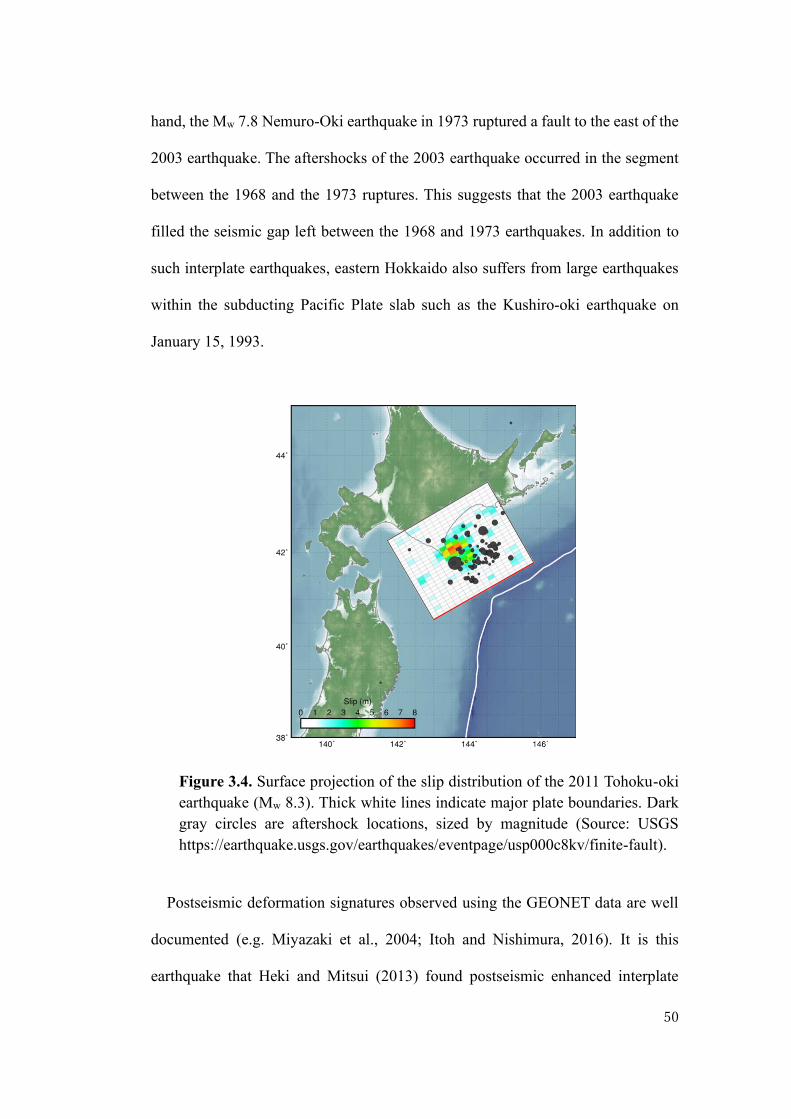
3.1.3 The 2003 Tokachi-oki Earthquake (Mw 8.3)

On September 25, 2003, a large interplate earthquake occurred near Hokkaido,

Japan, as the result of shallow thrust faulting on or near the plate interface between

the overriding Okhotsk Plate (or North American Plate) and the subducting Pacific

Plate. The epicenter was in the same location as the 1952 Tokachi-oki earthquake

and could be considered as the recurrence of the 1952 event, although their slip

distributions are a little different. Based on the analysis of the aftershock

distribution by Takahashi and Kasahara (2004), the source region of the 2003 event

is slightly smaller than that of the 1952 event.

In this region, the Pacific Plate is moving west-northwest at a velocity of about

91 mm/yr relative to the Okhostk Plate (Argus et al., 2011), subducting beneath

Japan at the Japan Trench. This earthquake generated tsunami with the largest

height of ~4 m (Tanioka et al., 2004). The coseismic slip distribution of the 2003

earthquake by USGS (Figure 3.4) indicates thrust faulting with a shallow dip angle

(strike= 240.0°, dip = 17.0°) of a fault plane with the length 272 and width 227 km.

Before the 2003 Tokachi-oki earthquake, eastern Hokkaido experienced many

large interplate earthquakes. Earthquakes with Mw 8.2 and Mw 7.7 occurred in 1968

and 1994, respectively, to the southwest of the 2003 earthquake rupture area. The

1994 earthquake ruptured the southern half of the 1968 rupture area. On the other

50

hand, the Mw 7.8 Nemuro-Oki earthquake in 1973 ruptured a fault to the east of the

2003 earthquake. The aftershocks of the 2003 earthquake occurred in the segment

between the 1968 and the 1973 ruptures. This suggests that the 2003 earthquake

filled the seismic gap left between the 1968 and 1973 earthquakes. In addition to

such interplate earthquakes, eastern Hokkaido also suffers from large earthquakes

within the subducting Pacific Plate slab such as the Kushiro-oki earthquake on

January 15, 1993.

Figure 3.4. Surface projection of the slip distribution of the 2011 Tohoku-oki

earthquake (Mw 8.3). Thick white lines indicate major plate boundaries. Dark

gray circles are aftershock locations, sized by magnitude (Source: USGS

https://earthquake.usgs.gov/earthquakes/eventpage/usp000c8kv/finite-fault).

Postseismic deformation signatures observed using the GEONET data are well

documented (e.g. Miyazaki et al., 2004; Itoh and Nishimura, 2016). It is this

earthquake that Heki and Mitsui (2013) found postseismic enhanced interplate

51

coupling, for the first time, at the segments adjacent northeastward and

southwestward to the ruptured segment.

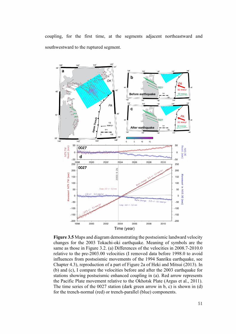
Figure 3.5 Maps and diagram demonstrating the postseismic landward velocity

changes for the 2003 Tokachi-oki earthquake. Meaning of symbols are the

same as those in Figure 3.2. (a) Differences of the velocities in 2008.7-2010.0

relative to the pre-2003.00 velocities (I removed data before 1998.0 to avoid

influences from postseismic movements of the 1994 Sanriku earthquake, see

Chapter 4.3), reproduction of a part of Figure 2a of Heki and Mitsui (2013). In

(b) and (c), I compare the velocities before and after the 2003 earthquake for

stations showing postseismic enhanced coupling in (a). Red arrow represents

the Pacific Plate movement relative to the Okhotsk Plate (Argus et al., 2011).

The time series of the 0027 station (dark green arrow in b, c) is shown in (d)

for the trench-normal (red) or trench-parallel (blue) components.

52

Figure 3.5 shows the maps and diagram similar to Figure 3.2 for the 2003

Tokachi-oki earthquake. I selected the GNSS stations with landward velocity

changes located along the Pacific coast of the northernmost Honshu (stations with

green vectors in Figure 3.5a, 0153, 0156, 0158, 0162, 0027, 0539 from north to

south). Figure 3.5b, c shows interseismic velocities before and after the earthquake.

Here I used the F3 solution and followed the procedures in Heki and Mitsui (2013),

i.e., I fixed the Kamitsushima station, Kyushu, Japan, which is not much different

from the frame fixed to the Okhotsk Plate used for the 2011 earthquake (Figure 3.2).

In Figure 3.5d, I show time series of the trench-normal (red) and trench-parallel

(blue) components for the 0027 station. There I can see the increased landward

movement of 5.3 mm/yr. Similar time series from two additional stations are given

in Figure 3.6.

53

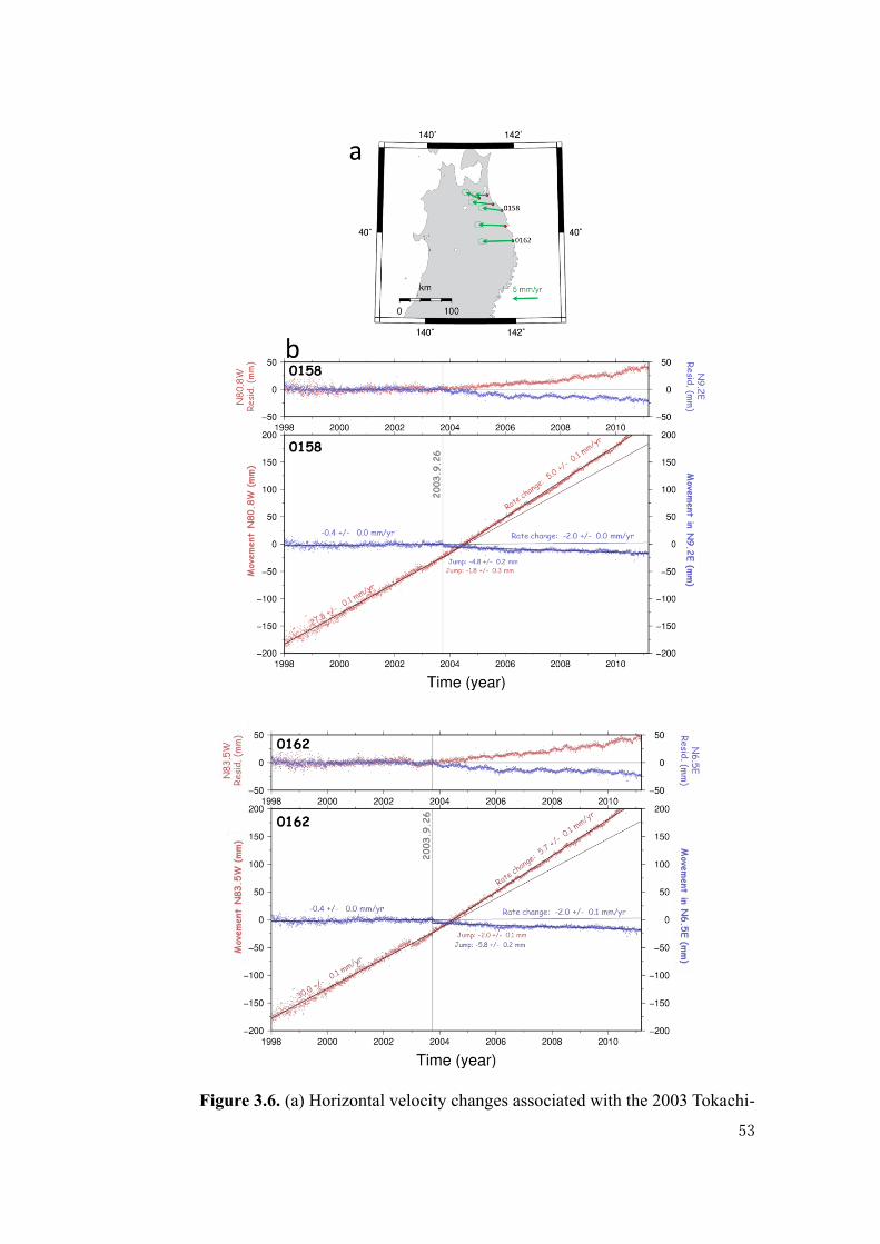
Figure 3.6. (a) Horizontal velocity changes associated with the 2003 Tokachi-

54

oki earthquake (same as stations with green arrows in Figure 3.5a). In (b), we

show time series of horizontal positions of the two stations 0158 and 0162

before and after the earthquake.

As reported in Heki and Mitsui (2013), I also found that the velocity in the trench-

parallel direction (N9.0E) has also changed the rate by -4.0±0.1 mm/yr. This reflects

the slight counterclockwise rotation of the velocity as recognized by comparing

Figures 3.5b and 3.5c. This might be due to postseismic viscous relaxation

occurring as a slow movement away from the fault (together with the trenchward

movement), which is visible in the numerical simulation results given in Figure

1.7b. Melnick et al. (2017), in their Figure 4, also shows that similar outward

movements are reproduced as a result of vertical axis crustal rotation.

As described earlier, Mavromatis et al. (2014) suggested that this landward

velocity change indicates the termination of the postseismic trenchward movement

caused by the 1994 Mw 7.6 Sanriku-oki earthquake (Heki et al., 1997). However,

this cannot be a significant factor partly because their model does not explain the

landward velocity change on the other side (easternmost Hokkaido) after the 2003

earthquake (Figure 3.5a).

Additional evidence comes from the velocity of 0027 prior to the 2003

earthquake (Figure 3.7). In order to confirm the influence of the postseismic

movement of the 1994 Sanriku-oki earthquake on the coseismic velocity changes

of the 2003 Tokachi-oki earthquake at stations in NE Honshu, I plot the baseline

length (distance) between the 0027 station (Figure 3.5) on the Pacific coast and the

0184 station on the Japan Sea coast.

55

Figure 3.7. The change of the baseline length connecting the 0027 and 0184

stations between the 1994 Sanriku-oki and 2003 Tokachi-oki earthquakes (the

F3 solution not available before 1996 March). Slopes are estimated in different

time windows of 1-1.5 years. The vertical error bars indicate 2 uncertainties.

This demonstrates that significant influence of the postseismic crustal movement

extends only until ~1998.

In Figure 3.7, the time series are modeled with lines with breaks at 1997.0, 1998.0,

1999.0, 2000.5, 2002.0. In 1996-1998, the distance does not show significant

changes due possibly to the balance of the landward (interseismic strain) and

oceanward (postseismic movement of the 1994 event) velocities of 0027. As the

latter decay, the slope becomes stationary. In fact, the effect of postseismic transient

of the 1994 Sanriku-oki earthquake remains dominant only until 1997-1998. I

excluded data before 1998.0 in deriving the pre-2003 velocity (Figure 3.5d).

Therefore, the postseismic transient of the 1994 earthquake would not significantly

affect the estimated velocity increases in 2003 September.

3.2 The cases in Chile

3.2.1 Tectonic setting in Central and Northern Chile

Chile is a country located along the west coast of South America and situated

56

in one of the world's most active tectonic regions. This long but narrow country lies

on or is close to four tectonic plates: The South American Plate, the Nazca Plate,

the Scotia Plate, and the Antarctic Plate. The Chile subduction zone, stretching more

than 3500 km, is segmented by the subduction of the Chile Rise and by the Juan

Férnandez Ridge.

The Chile Rise is an active spreading center that indicates the margin between

the Nazca Plate to the north and the Antarctic Plate to the south. The Chile Rise first

collided with the continent south of 48° S, in the Tierra del Fuego, at ~14 Ma and

then migrated northward to the current location of triple junction. Consequently, the

span of the Antarctic–South America subduction zone has increased during this

period (Cande and Leslie 1986).

The Juan Férnandez Ridge is a gentle topographic swell created by a series of

disconnected, large seamounts. The most notable seamounts on the oceanic plate

near the central Chile trench are the O'Higgins guyot and O'Higgins seamount,

located in the easternmost portion of Juan Férnandez Ridge before subduction. The

Juan Férnandez Ridge has been colliding with the Chilean margin in the north (at

∼20°S) since ~22 Ma, and the collision front migrated southward to the current

collision zone offshore Valparaíso (∼32.5°S) (Yáñez et al., 2001).

The eastern side of the Nazca Plate forms the Peru-Chile Trench, the

convergent margin with the overriding South American Plate, and the Andean

Mountain Range is the continental arc made by this plate convergence. The Nazca

Plate currently moves eastward relative to the South American Plate with a velocity

of ~74 mm/year (Argus et al. 2011). The direction of the movement is almost

perpendicular to the trench. The age of the Nazca Plate in North and Central Chile

57

ranges from ∼37 Ma to ∼48 Ma (Müller et al.1997).

Tomographic model of the seismic wave velocity structure of the mantle in the

area of the 2010 M8.8 Maule earthquake and surrounding regions (Pesicek et al.,

2012) shows that the length of the slab is ~1,100 km. On the other hand, the length

of the Nazca slab under South America from 6°S to 32°S is also ~1,100 km from

tomographic studies (Scire et al., 2017).

3.2.2 The 2010 Maule Earthquake (Mw 8.8)

Fast convergence between the Nazca and the South American Plates causes

recurrent megathrust earthquakes along the Peru-Chile Trench off the Pacific coast

of South America. The 2010 February Maule earthquake, one such event in central

Chile, filled the seismic gap lasting since the 1835 Conception earthquake. In

addition to the co- and postseismic crustal deformation of this earthquake reported

in Vigny et al. (2011), Moreno et al. (2012), and Klein et al. (2016), Melnick et al.

(2017) reported postseismic increase of the landward velocities of stations located

to the north of the rupture. They further suggested that such enhanced coupling may

have triggered the occurrence of the 2015 Illapel earthquake (Mw 8.3) to the north

of the 2010 rupture.

Klein et al. (2016) reported large-scale postseismic oceanward movements of

GNSS stations around the ruptured segment, and it can be seen in velocity changes

by the 2010 earthquake in Figure 3.8a. We also can see that stations located to the

north of the 2010 rupture show clear signatures of enhanced interplate coupling

(green vectors in Figure 3.8a). The velocities of these GNSS stations before and

after the earthquake are shown in Figure 3.8b and c, respectively. Figure 3.8d shows

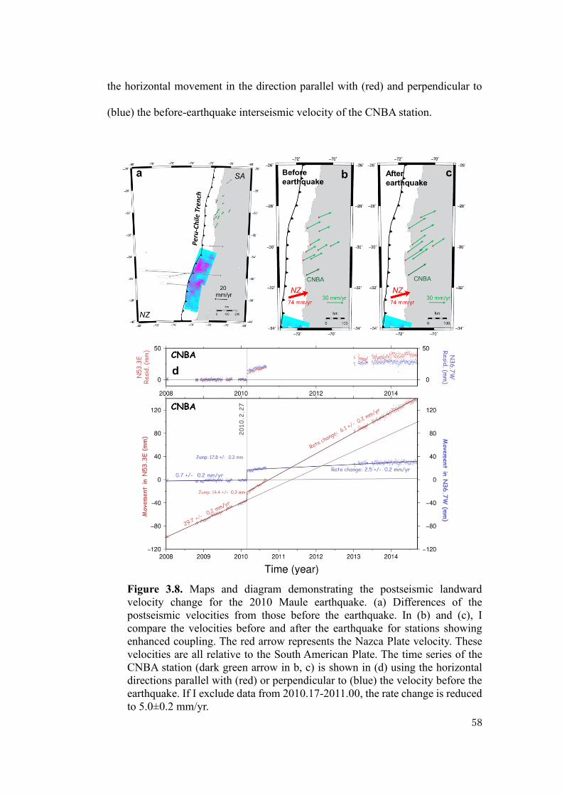
58

the horizontal movement in the direction parallel with (red) and perpendicular to

(blue) the before-earthquake interseismic velocity of the CNBA station.

Figure 3.8. Maps and diagram demonstrating the postseismic landward

velocity change for the 2010 Maule earthquake. (a) Differences of the

postseismic velocities from those before the earthquake. In (b) and (c), I

compare the velocities before and after the earthquake for stations showing

enhanced coupling. The red arrow represents the Nazca Plate velocity. These

velocities are all relative to the South American Plate. The time series of the

CNBA station (dark green arrow in b, c) is shown in (d) using the horizontal

directions parallel with (red) or perpendicular to (blue) the velocity before the

earthquake. If I exclude data from 2010.17-2011.00, the rate change is reduced

to 5.0±0.2 mm/yr.

59

The red component shows velocity increase of 6.1±0.2 mm/yr. There is some

misfit of the data to the straight line in the 2010 data. This suggests that the

postseismic landward velocity increase is somewhat larger immediately after the

earthquake than that after a few years. However, such a non-linear movement

cannot be seen in the two Japanese cases discussed in sections 3.1.2 and 3.1.3.

It is also interesting to see that the blue component shows the postseismic slow

movement away from the fault, a feature also observed after the 2003 Tokachi-oki

earthquake (Figure 3.5d). The stations in Figure 3.8b and 3.8c showing enhanced

landward velocities, including CNBA, suffer from data gaps up to two years (Figure

2.6). Additional time series of two stations are given in Figures 3.9. Change in

seismicity in the region showing enhanced landward movements are discussed later

in Chapter 5.2.

60

Figure 3.9. (a) Horizontal velocity changes by the 2010 Maule earthquake

61

(same as stations with green arrows in Figure 3.8a). In (b) we show time series

of horizontal components at the two stations BTO1 and JUNT. These stations

suffer from data gaps lasting for ~2 years.

3.2.3 The 2014 Iquique Earthquake (Mw 8.2)

The 2014 April Iquique earthquake occurred at a segment near the Peru-Chile

border. This segment has been known as the north Chilean seismic gap with the last

rupture by the 1877 Iquique earthquake (Mw 8.6) (Kelleher, 1972). Postseismic

trenchward movements occur near the ruptured fault as the combined effect of the

afterslip and the viscoelastic relaxation (Hoffmann et al., 2018). Figure 3.10a

suggests that the stations located to the south of 21 S, as well as one station AREQ

to the north, are not affected by such postseismic trenchward movements.

Figure 3.10d shows the SRGD station to the south of the rupture, showing small

landward velocity increase of 2.8 mm/yr by the 2014 earthquake. On the northern

side, AREQ shows the increase of 2.9 mm/yr. Both SRGD and AREQ stations are

located at distances comparable to the fault length from the SE and NW edges of

the fault. The time series of AREQ and an additional station to the south of the

rupture are given in Figure 3.11.

Large interplate earthquakes occurred recently around the 2014 Iquique

earthquake. To the north, the southern Peru earthquake (Mw 8.4) occurred near

Arequipa in 2001, being followed by postseismic deformation continuing for at

least two years (Perfettini et al., 2005). The rupture area of the 2001 earthquake

seems to be coupled again a decade after the earthquake (Villegas-Lanza et al.,

2016). I expect that the increasing of landward velocity at AREQ station after 2014

was not much influenced by the decay of the postseismic movement of the 2001

event.

62

To the south, the 2007 Tecopilla earthquake (Mw 7.7) (Schurr et al., 2012) and

the 1995 Antofagasta earthquake (Mw 8.1) (Pritchard et al., 2002) did not

significantly change the slip deficit in the studied region. Strong interplate coupling

is confirmed in the 2014 Iquique earthquake focal region prior to the earthquake

(Métois et al., 2013; Li et al., 2015). Hence, I think the influences from the

postseismic movements of these earthquakes to the landward velocity change

following the 2014 Iquique earthquake are small.

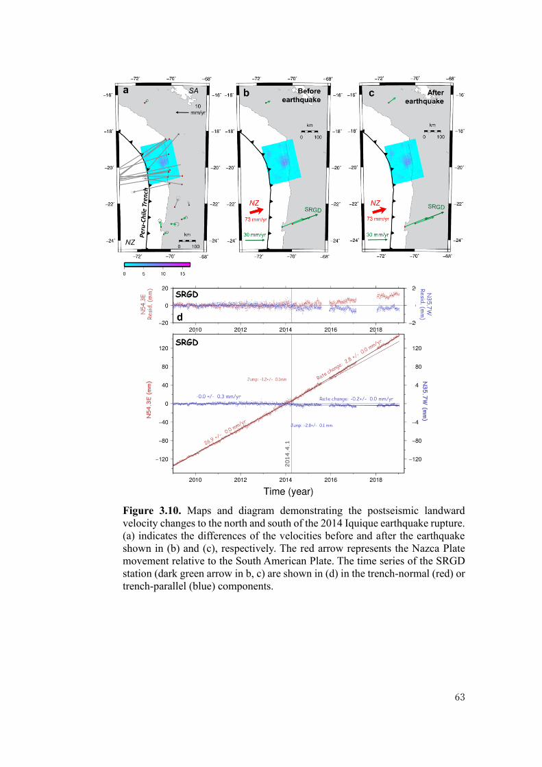
63

Figure 3.10. Maps and diagram demonstrating the postseismic landward

velocity changes to the north and south of the 2014 Iquique earthquake rupture.

(a) indicates the differences of the velocities before and after the earthquake

shown in (b) and (c), respectively. The red arrow represents the Nazca Plate

movement relative to the South American Plate. The time series of the SRGD

station (dark green arrow in b, c) are shown in (d) in the trench-normal (red) or

trench-parallel (blue) components.

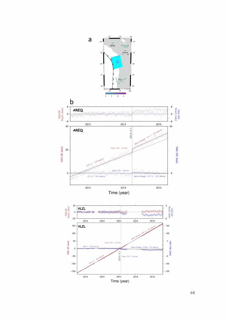
64

65

Figure 3.11. (a) Horizontal velocity changes by the2014 Iquique earthquake

(same as stations with green arrows in Figure 3.10a). In (b) we show time

series of the two stations AREQ and VLZL.

3.3 The case in Sumatra

3.3.1 Tectonic setting in Southwest Sumatra

The Sunda Arc, which extends more than 4000 km, is formed by the subduction

of the Indo-Australian Plate (or the Australian Plate) beneath the Eurasian Plate (or

the Sundaland Plate). This arc ranges from the Andaman Sea in the northwest to the

Banda Sea in the east. The region west of the Sumatra Island is one of the most

seismically active and tectonically complex regions on the Earth. There are some

debates regarding whether the Sundaland Plate is moving as a distinct lithospheric

block or can be regarded as a stable continuation of its northward-neighboring

Eurasian Plate (Simons et al., 2007).

The Sunda Arc is characterized by a high degree of volcanic activity of mostly

andesitic composition (Curray, 1989). In the Sumatra subduction zone, which is a

part of the Sunda Arc, the oceanic plate subducts beneath the landward plate

obliquely (~40° at 2°N) with a convergence rate that varies along the trench from

~60 mm/yr at 6°S to ~52 mm/yr at 2°N (Prawirodirdjo et al., 2000). The subduction

system has been active since at least the Oligocene and is much influenced by the

late Eocene collision of the Indian subcontinent with Eurasia (Hamilton 1988). The

age of the subducting plate varies from 40 Ma to 80 Ma (Muller et al., 2008), with

the youngest oceanic crust subducting to the east of the Nias Island in northern

Sumatra. To the west of the Sumatra Island, the forearc ridge emerges and forms an

island chain, extending from the Simelue Islands in the northwest to the Enggano

66

Island in the southeast. To the south of the Java Island, this forearc ridge submerges

below the sea level (Susilo Hadi et al., 2009). Tomographic model of the mantle in

the area of the 2007 Mw 8.4 Bengkulu earthquake and surrounding regions by

suggests that the length of the slab is ~700 km (Hafkenscheid et al., 2001).

3.3.2 The 2007 Bengkulu Earthquake (Mw 8.4)

The 2007 September Bengkulu earthquake occurred within the southern

Sumatra subduction zone as a result of the oblique convergence of the two plates.

In this region, the Australian Plate moves northeastward with respect to the

Sundaland Plate at a velocity of about ~60 mm/yr (Argus et al. 2011). USGS Finite

fault modelling indicates that the fault of this earthquake slipped over an area

approximately 300 km long (along strike) by 110 km wide (in the down-dip

direction, Figure 3.12).

Figure 3.12. Surface projection of the slip distribution of the 2007 Bengkulu

Earthquake (Mw 8.4) (Source: USGS https://earthquake.usgs.gov/ earthquakes/

eventpage/ official20070912111026830_34/finite-fault).

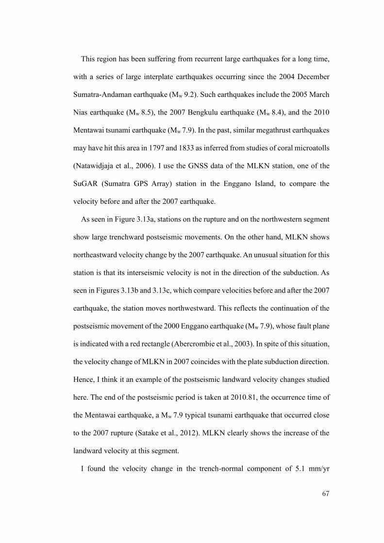
67

This region has been suffering from recurrent large earthquakes for a long time,

with a series of large interplate earthquakes occurring since the 2004 December

Sumatra-Andaman earthquake (Mw 9.2). Such earthquakes include the 2005 March

Nias earthquake (Mw 8.5), the 2007 Bengkulu earthquake (Mw 8.4), and the 2010

Mentawai tsunami earthquake (Mw 7.9). In the past, similar megathrust earthquakes

may have hit this area in 1797 and 1833 as inferred from studies of coral microatolls

(Natawidjaja et al., 2006). I use the GNSS data of the MLKN station, one of the

SuGAR (Sumatra GPS Array) station in the Enggano Island, to compare the

velocity before and after the 2007 earthquake.

As seen in Figure 3.13a, stations on the rupture and on the northwestern segment

show large trenchward postseismic movements. On the other hand, MLKN shows

northeastward velocity change by the 2007 earthquake. An unusual situation for this

station is that its interseismic velocity is not in the direction of the subduction. As

seen in Figures 3.13b and 3.13c, which compare velocities before and after the 2007

earthquake, the station moves northwestward. This reflects the continuation of the

postseismic movement of the 2000 Enggano earthquake (Mw 7.9), whose fault plane

is indicated with a red rectangle (Abercrombie et al., 2003). In spite of this situation,

the velocity change of MLKN in 2007 coincides with the plate subduction direction.

Hence, I think it an example of the postseismic landward velocity changes studied

here. The end of the postseismic period is taken at 2010.81, the occurrence time of

the Mentawai earthquake, a Mw 7.9 typical tsunami earthquake that occurred close

to the 2007 rupture (Satake et al., 2012). MLKN clearly shows the increase of the

landward velocity at this segment.

I found the velocity change in the trench-normal component of 5.1 mm/yr

68

following the 2007 Bengkulu earthquake (Figure 3.13d). Unlike other cases,

MLKN is located quite close to the southeastern edge of the fault of the 2007

earthquake. In this earthquake, the afterslip occurred mainly in the northwest part

of the fault, which made the postseismic signals weak at MLKN. Lubis et al. (2012)

calculated postseismic crustal movements of the 2007 earthquake by the

viscoelastic relaxation, and the results showed insignificant movement around the

MLKN station, and this support our interpretation that the velocity change of

MLKN comes from the landward increased velocity of the 2007 earthquake.

This region is thought to be a part of the Sunda Strait seismic gap. Mignan et al.

(2006) suggested that this area has remarkable accelerated seismic moment release

similar to the area where maximum slip occurred during the 2004 Sumatra-

Andaman earthquake. Hanifa et al. (2014) pointed out that the region off the

southwestern coast of Java is a seismic gap with a high probability of future

earthquakes. The enhanced coupling after the 2007 Bengkulu earthquake might

contribute to accelerated strain accumulation in those segments.

69

Figure 3.13. Maps and diagram showing the increased landward velocity after

the 2007 Bengkulu earthquake. (a) Differences of the velocities (relative to the

Sunda Plate) between periods before and after the earthquake shown in (b) and

(c), respectively. The red arrow represents the Australian Plate subduction

relative to the Sunda Plate. The red rectangle indicates the fault plane of the

2000 Enggano earthquake (Mw 7.9). The time series of the MLKN station is

shown in (d) using the horizontal directions parallel with (red) or perpendicular

to (blue) the subduction direction.

3.4 The case in Mexico

3.4.1 Tectonic Setting of Mexico

Mexico is located on The Middle America subduction zone, where the Rivera and

70

The Cocos Plates subduct beneath the North American and Caribbean Plates along

the Middle America Trench. Around 30–28 Ma, a larger tectonic plate called the

Farallon Plate, gradually split into several fragments, including the Rivera and

Cocos Plate. This split began when the East Pacific Rise to interact with the North

American Plate (Atwater and Stock, 1998). Cocos Plate is a relatively young

oceanic plate (10–25 Ma) which subducts along the Middle America Trench at

variable convergence rates 50 to 90 mm/yr (Manea et al., 2013).

3.4.2 The 2012 Oaxaca Earthquake (Mw 7.4)

Several significant earthquakes occurred in the region near the 2012 March

Oaxaca earthquake, e.g. the 1932 Mw 7.9 earthquake, the 1995 Mw 8.0 earthquake,

and the 1985 Mw 8.1 earthquake (Kanamori et al., 1993; Courboulex et al., 1997).

For this earthquake, I could find only one station suitable for the present study, the

OXPE station (Figures 3.14a, b), with meaningful time span before and after the

earthquake and with position near the 2012 rupture. Our result showed a small

increase of the landward component of the horizontal velocity of ~4.1 mm/yr

(Figure 3.14c). This station is located at a distance comparable to the fault length

from the SE edge of the fault.

It is difficult to know if earthquakes before the 2012 Oaxaca earthquake

influence landward velocity change because of the lack of enough GNSS data. The

last major earthquake that occurred near the OXPE station, is a M7.5 earthquake in

1999 (Segou and Parsons, 2018). Considering the time between the two earthquakes,

the decay of its postseismic crustal deformation would not significantly influence

the results shown in Figure 3.14.

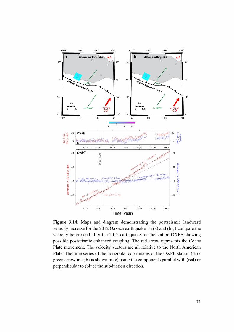
71

Figure 3.14. Maps and diagram demonstrating the postseismic landward

velocity increase for the 2012 Oaxaca earthquake. In (a) and (b), I compare the

velocity before and after the 2012 earthquake for the station OXPE showing

possible postseismic enhanced coupling. The red arrow represents the Cocos

Plate movement. The velocity vectors are all relative to the North American

Plate. The time series of the horizontal coordinates of the OXPE station (dark

green arrow in a, b) is shown in (c) using the components parallel with (red) or

perpendicular to (blue) the subduction direction.

72

Chapter 4: Discussion

4.1 Overview of the six cases

I reported six cases in four different subduction zones suggesting the post-

megathrust occurrence of landward increase of forearc velocity on the segments

adjacent along-strike to the ruptured segment. They are not easily explained by

conventional interpretations with postseismic processes such as afterslip and local

scale viscous relaxation. I first revisited the 2003 Tokachi-oki and the 2011 Tohoku-

oki earthquakes in NE Japan reported by Heki and Mitsui (2013). I then studied the

2010 Maule earthquake, Chile, for which Melnick et al. (2017) reported increased

landward movements north of the rupture. I also studied the velocity changes

associated with the 2014 Iquique earthquake in northern Chile, originally found by

Hoffmann et al. (2018). I newly found the signatures for the 2007 Bengkulu

earthquake (Southwestern Sumatra), and the 2012 Oaxaca earthquake (Mexico).

The six examples include the two cases, 2011 Tohoku-oki and 2007 Bengkulu

earthquakes, where interseismic velocities deviate largely from relative plate

subduction directions. Such deviations are due to long-lasting postseismic crustal

movements of past earthquake, i.e. 2003 Tokachi-oki and the 2000 Enggano

earthquakes, respectively. Even in these cases, the velocity changes nearly align

with the plate subduction directions. I also carefully evaluated the leakage of the

decaying trenchward postseismic crustal movements of past large nearby

73

earthquakes into the inferred landward velocity increases.

In addition to landward velocity increase, a trench-parallel velocity change was

found after the 2003 Tokachi-oki earthquake (Heki and Mitsui, 2013). Also, in the

2010 Maule earthquake, the changes of the velocities are somewhat deviated

counterclockwise from the plate subduction direction (Figure 3.8a). Such changes

could be driven by postseismic viscous relaxation.

Vertical velocities may also have changed at stations showing enhanced landward

velocities. Because of the larger noises in vertical component, I cannot draw

decisive conclusions for them (Figure 2.14). We should revisit the problem after

data with enough time span become available in the future.

In addition to the six cases studied here, I looked for similar increase signatures

for other megathrusts in various subduction zones. They include the 2004 December

Sumatra-Andaman earthquake (Mw 9.2) and the 2005 March Nias earthquake (Mw

8.6) (Figure 1.5). The search was not successful in these cases simply due to the

lack of enough time span of pre- and postseismic data from GNSS stations in

appropriate places. The movements of the SuGAR stations are well documented by

e.g., Feng et al. (2015). Below I summarize the situation in Sumatra.

The three SuGAR stations (PSMK, PTLO, PBAI) in islands to the northwest of

Sumatra started working well before the 2004 Sumatra-Andaman earthquake and

may have recorded enhanced landward velocities following that event. However,

the 2005 March Nias earthquake occurred before we can confirm its signature, and

their velocity changed trenchward due to the postseismic movements by the 2005

event. Three SuGAR stations (MSAI, PSKI, BSAT) off the middle Sumatra started

operation before 2004, but they were not close enough to the 2005 rupture and did

74

not show significant post-2005 landward velocity change. It is a pity because it is

likely that these two earthquakes caused landward velocity increases in the Sumatra

subduction zone. In fact, a series of Mw>7 earthquakes occurred in the segments to

the southwest of these two earthquakes (Haridhi et al., 2018) suggesting accelerated

interplate strain buildup there.

A similar situation applies for the 2015 Illapel earthquake (Mw 8.3), in central

Chile (Figure 1.5). For example, the COPO station is in the region suitable to study

increased coupling by the 2015 earthquake, but its observation data are not available

after 2015.

4.2 Spatial decay of the enhanced coupling

The enhanced coupling may encourage future failures in the neighboring

segments. For example, earthquakes such as the 2015 Illapel earthquake (Mw 8.3)

and the 2016 Chiloé earthquake (Mw 7.6), occurred to the north and south of the

2010 Maule earthquake, respectively, may have been triggered by the enhanced

coupling caused by the 2010 Maule event (Mw 8.8) (Melnick et al., 2017; Ruiz et

al., 2017). To further discuss this issue, it is important to know the spatial and

temporal decay of the enhanced coupling.

In Chapter 3, I did not pay much attention to the relationship between amounts

of the velocity changes and distances from the ruptured faults. In Figure 4.1, I plot

the landward velocity increases as a function of the distance from the center of the

fault for the 2003 Tokachi-oki, 2011 Tohoku-oki, and the 2010 Maule earthquakes.

For the Tohoku-oki case, postseismic trenchward movements seem to prevail from

the rupture area as far to the northeast as ~100 km from the fault edge. According

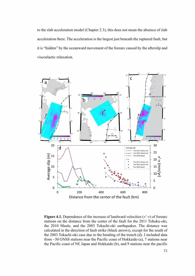
75

to the slab acceleration model (Chapter 2.3), this does not mean the absence of slab

acceleration there. The acceleration is the largest just beneath the ruptured fault, but

it is “hidden” by the oceanward movement of the forearc caused by the afterslip and

viscoelastic relaxation.

Figure 4.1. Dependence of the increase of landward velocities (v’-v) of forearc

stations on the distance from the center of the fault for the 2011 Tohoku-oki,

the 2010 Maule, and the 2003 Tokachi-oki earthquakes. The distance was

calculated in the direction of fault strike (black arrows), except for the south of

the 2003 Tokachi-oki case due to the bending of the trench (d). I included data

from ~30 GNSS stations near the Pacific coast of Hokkaido (a), 7 stations near

the Pacific coast of NE Japan and Hokkaido (b), and 9 stations near the pacific

76

coast of central Chile (c). The average slips in both along-strike directions from

the fault centers are obtained from the slip models from USGS. Broken curves

are hypothetical smooth models.

For the 2011 Tohoku-oki case, the landward velocity changes prevail for stations

farther than ~100 km from the fault edge. Such an increase is confirmed to continue

as far as ~650 km from the fault center, but it is not clear if it extends beyond that

point due to the lack of data. For the 2010 Maule case, I have data only beyond 500

km from the fault center. Probably, the true maximum landward velocity increase

for this event would exist somewhere with distance < 500 km. For this earthquake,

the data are available as far as 800 km, and the velocity increases seem to decay

gradually for distance range 500-800 km. For the 2003 Tokachi-oki case, landward

increase appears in the stations closer to the fault, and its maximum occurs only

~100 km from the fault edge. From these three cases, the landward velocity increase

seems to extend at least as far as ~1/2 the fault lengths beyond the fault edges.

If such a landward velocity increase causes increased interplate coupling, large

earthquakes may be encouraged in future in “affected segments”, e.g. the southern

Kuril Islands and in central Chile. It would be reasonable to consider that the

enhanced interplate coupling to the north of the Maule rupture has triggered the

2015 Mw 8.3 Illapel earthquake (see Figure 4.1c for position).

D’acquisto et al. (2020) used the velocity-driven 3D mechanical finite element

models to quantify and analyze the deformation that produces landward motion by

the viscous relaxation of the mantle wedge and the deep afterslip. Their results show

increased postseismic landward motion of up to ~6.1 mm/yr at (trench-parallel)

distances >450 km from the middle of the ruptured asperity. They conclude that

enhanced landward motion is generated by in-plane elastic bending of the

77

overriding plate and mantle wedge in response to oceanward motion of lithosphere

around the rupture zones. Their results are also consistent with the observations in

Central Chile. Melnick et al. (2017) used a large-scale three-dimensional

thermomechanical model to simulate viscoelastic relaxation of the mantle to

explain continental-scale velocity changes. Their model also reproduces the

observed landward velocity increase.

4.3 Temporal decay of the enhanced coupling

Another important aspect is the temporal decay. According to the slab

acceleration model (Chapter 2.3), The enhanced coupling decays as the interplate

coupling Fc returns to the pre-earthquake state. Such a recovery time may depend

on the earthquake magnitude, i.e. the larger the magnitude, the longer the period for

the recovery of interplate coupling. In the time series of trench-normal movements

(Figures in Chapter 3), temporal decays are not very evident, i.e. landward

movements show simple increased linear trends without notable curvatures. For the

2010 Maule, the time series has a curvature immediately after the earthquake, but

we do not see a curvature after the data gap (Figure 3.8). Here I confirm this

numerically.

I set up the moving 1-year time period for the linear regression to see possible

temporal change in slope (Figure 4.2). This analysis shows that velocity changes

are either higher or lower in the first few years due to postseismic transients. Gray

arrows in Figure 4.2 indicate rough length of significant postseismic transients

given in past literatures. After these years, the velocity changes seem to remain

stable.

78

Figure 4.2 Interseismic landward velocity change estimated within moving 1-year time windows (a-f). Horizontal coordinates of the

green circles show the centers of the time windows. Gray arrows represent the duration of postseismic decay based on previous studies.

In (c) and (e), I exclude data after significant earthquakes occurred nearby (black dashed line). After periods of instability, the rate

becomes stationary for subsequent years. In the two Chilean cases (c, d), data gaps make the rate change unstable.

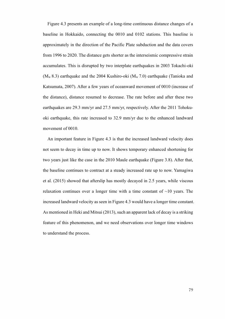
79

Figure 4.3 presents an example of a long-time continuous distance changes of a

baseline in Hokkaido, connecting the 0010 and 0102 stations. This baseline is

approximately in the direction of the Pacific Plate subduction and the data covers

from 1996 to 2020. The distance gets shorter as the interseismic compressive strain

accumulates. This is disrupted by two interplate earthquakes in 2003 Tokachi-oki

(Mw 8.3) earthquake and the 2004 Kushiro-oki (Mw 7.0) earthquake (Tanioka and

Katsumata, 2007). After a few years of oceanward movement of 0010 (increase of

the distance), distance resumed to decrease. The rate before and after these two

earthquakes are 29.3 mm/yr and 27.5 mm/yr, respectively. After the 2011 Tohoku-

oki earthquake, this rate increased to 32.9 mm/yr due to the enhanced landward

movement of 0010.

An important feature in Figure 4.3 is that the increased landward velocity does

not seem to decay in time up to now. It shows temporary enhanced shortening for

two years just like the case in the 2010 Maule earthquake (Figure 3.8). After that,

the baseline continues to contract at a steady increased rate up to now. Yamagiwa

et al. (2015) showed that afterslip has mostly decayed in 2.5 years, while viscous

relaxation continues over a longer time with a time constant of ~10 years. The

increased landward velocity as seen in Figure 4.3 would have a longer time constant.

As mentioned in Heki and Mitsui (2013), such an apparent lack of decay is a striking

feature of this phenomenon, and we need observations over longer time windows

to understand the process.

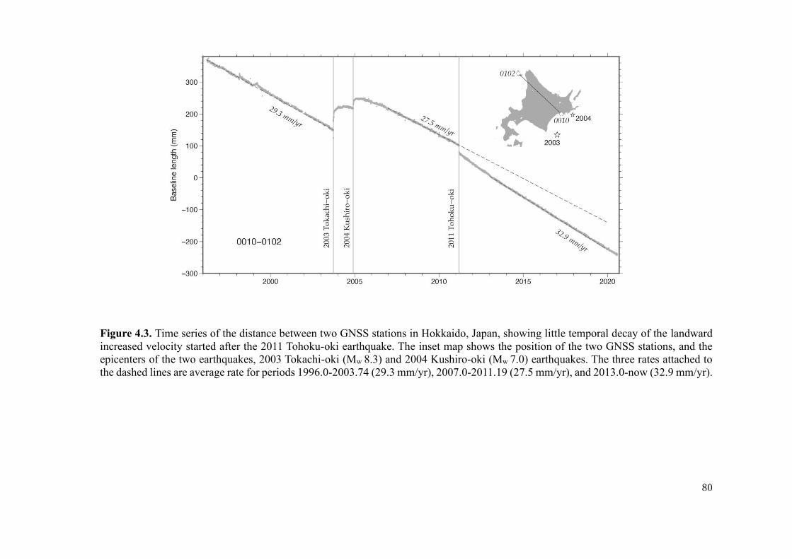
80

Figure 4.3. Time series of the distance between two GNSS stations in Hokkaido, Japan, showing little temporal decay of the landward

increased velocity started after the 2011 Tohoku-oki earthquake. The inset map shows the position of the two GNSS stations, and the

epicenters of the two earthquakes, 2003 Tokachi-oki (Mw 8.3) and 2004 Kushiro-oki (Mw 7.0) earthquakes. The three rates attached to

the dashed lines are average rate for periods 1996.0-2003.74 (29.3 mm/yr), 2007.0-2011.19 (27.5 mm/yr), and 2013.0-now (32.9 mm/yr).

81

4.4 Forearc station velocities and slab velocities

Heki and Mitsui (2013) hypothesized that postseismic enhancements of the

interplate coupling may reflect the accelerated rate of the slab subduction u’-u in

response to the modified balance of forces acting on the subducting slab (Figure

2.15). Actually, what is observed is the change in velocity of forearc GNSS stations

v’-v, and it is necessary to convert v’-v to u’-u. Generally, v becomes larger if

interplate coupling is stronger, but v never exceeds u. I here inferred the ratio v/u

(0 v/u <1) by comparing the observed interseismic velocity of the GNSS station

and the subduction speed calculated by the MORVEL model (Argus et al., 2011).

For example, in the Maule earthquake, the velocity of the CNBA station observed

before (vCNBA) and after (v’CNBA) the earthquake, might be related to the

hypothetical slab acceleration u’Nazca-uNazca. This relationship can be formulated

using the subduction speed of the Nazca Plate vNazca relative to the South American

Plate at the Chile Trench, as follows,

u’Nazca-uNazca = (vNazca /vCNBA) × (v’CNBA -vCNBA) (6)

This conversion is applied to all cases except the Tohoku-oki and the Bengkulu

earthquakes. In these two cases, postseismic movements of nearby earthquakes in

recent past still influenced v and v’ (Figures 3.2 and 3.13), i.e. the 2003 Tokachi-oki

and the 2000 Enggano earthquakes, respectively. In Japan, I used the interseismic

velocities before the earlier earthquake (i.e. before 2003). For the MLKN station,

the data are not available before 2000, and so I used the average of interseismic

velocities in 2000-2007 of the five stations above the 2007 rupture (Figure 3.13a)

to infer vMLKN.

82

By such calculations, the acceleration of the slab subduction for the six cases

became, 22.0 mm/yr (2011 Tohoku-oki), 8.4 mm/yr (2003 Tokachi-oki), 10.4

mm/yr (2010 Maule), 6.6 mm/yr (2014 Iquique), 8.5 mm/yr (2007 Bengkulu), and

10.1 mm/yr (2012 Oaxaca). For the first four cases, I have data from multiple

stations and calculated the uncertainties in such velocity changes.

4.5 Comparison of the data with the slab acceleration model (Heki

and Mitsui, 2013)

Here I examine the slab acceleration model by Heki and Mitsui (2013) by

comparing the acceleration of the subduction speed inferred in the previous section

with the model predictions. The equation (2) suggests that the decrease in the

coupling Fc’-Fc determines the slab acceleration u’-u. The acceleration would hence

depend on Mw, because a larger earthquake would cause larger Fc’-Fc. Figure 4.4

compares de-trended time series of trench-normal movements of the forearc

stations for the six cases studied here, using a unified vertical axis. The figure shows

that the acceleration is larger for a case with a larger Mw, and the most significant

velocity increase appeared following the Mw 9.0 2011 Tohoku-oki earthquake.

83

Figure 4.4. Comparison of the increased landward velocities of GNSS stations

following six megathrust earthquakes studied here. I removed linear trends

before the earthquakes to facilitate the comparison of postseismic velocity

increases for the six cases. The vertical grey line, used as the origin, indicates

the earthquake occurrence times. The station names and the azimuths of the

displayed movements are given to the left, and the earthquake names and their

Mw are given to the right.

The surface velocity changes v’-v in Figure 4.4 are converted to slab velocity

changes u’-u, as discussed in the previous section. Figure 4.5a compares u’-u in

addition to v’-v as a function of Mw. There, smaller symbols show v'-v and u'-u at

individual stations for earthquakes where multiple stations are available. We can

see that a larger earthquake brings a larger change, both forearc (v) and slab (u)

velocities.

As discussed in Section 3, the loss of coupling Fc’– Fc would be proportional to

the coseismic slip averaged over the fault sav if we fix other parameters. Figure 4.5b

84

compares the slab acceleration with the average slip sav, calculated using the slip

data of USGS as shown in Figures 3.2, 3.5, 3.8, 3.10, 3.13, and 3.14. The

acceleration seems to show good correlation with sav considering that the value for

the 2010 Maule earthquake is probably an underestimate (Figure 4.1d). However,

it is not very clear if the two quantities are proportional considering the four

earthquakes with Mw8.5 are clustered at a down-left corner of the figure and do

not contribute to the evaluation of the linearity.

85

Table 4.1. Slab length for individual earthquake.

No Earthquake Slab length (km) W (km) Source

1 The 2011 Tohoku-oki (Mw 9.0) 1,075 2,150 Deal and Nolet (1999)

2 The 2010 Maule (Mw 8.8) 1,100 2,200 Pesicek, et al. (2012)

3 The 2003 Tokachi-oki (Mw 8.3) 1,075 2,150 Deal and Nolet (1999)

4 The 2007 Bengkulu (Mw 8.4) 700 1,400 Hafkenscheid, et al. (2001)

5 The 2014 Iquique (Mw 8.2) 1,100 2,200 Scire, et al. (2017)

6 The 2012 Oaxaca (Mw 7.4) 900 1,800 Husker and Davis (2009)

86

Table 4.1. Average slip for individual earthquake.

No. Earthquake Average

slip (m) Source

1 The 2011 Tohoku-oki (Mw 9.0) 7.97 https://earthquake.usgs.gov/earthquakes/eventpage/official20110311054624120_30/finite-

fault

2 The 2010 Maule (Mw 8.8) 5.14 https://earthquake.usgs.gov/earthquakes/eventpage/usp000c8kv/finite-fault

3 The 2003 Tokachi-oki (Mw 8.3) 0.80 https://earthquake.usgs.gov/earthquakes/eventpage/official20100227063411530_30/finite-

fault

4 The 2007 Bengkulu (Mw 8.4) 0.80 https://earthquake.usgs.gov/earthquakes/eventpage/usc000nzvd/finite-fault

5 The 2014 Iquique (Mw 8.2) 0.77 https://earthquake.usgs.gov/earthquakes/eventpage/official20070912111026830_34/finite-

fault

6 The 2012 Oaxaca (Mw 7.4) 0.63 https://earthquake.usgs.gov/earthquakes/eventpage/usp000jghj/finite-fault

87

Figure 4.5. (a) Comparison of the forearc acceleration, v'-v, and the slab acceleration, u'-u, for six different megathrust earthquakes with

Mw7.4-9.0. Different symbols indicate different subduction zones. Smaller symbols show values at individual stations for the cases with

multiple available stations. (b) Mw is replaced with the slips averaged over the faults (sav) in (b) and with sav/W, where W corresponds to

the length of the slab surface (see eq. 5). Error bars show the standard deviation of the averages of these velocity changes.

88

Equation (5) also suggests that the slab acceleration is inversely proportional to

W, the length the slab surface. Here I assumed that W is twice as long as the slab

lengths inferred from seismic tomography studies and compare u’-u and sav/W in

Figure 4.5c. Here I use the information on the lengths W, twice as long as the slab

length, i.e. 1,075 km for NE Japan (Deal and Nolet, 1999), 1,100 km for Chile

(Scire et al., 2017), 700 km for Sumatra (Hafkenscheid et al., 2001), and 900 km

for Mexico (Husker and Davis, 2009). Considering that the value for the Maule

event is underestimated, data in Figure 4.5c may suggest linearity. Nevertheless,

they are not enough to provide a firm support to the slab acceleration model by Heki

and Mitsui (2013), considering that 4 smaller earthquakes are clustered and do not

fully contribute to the evaluation of the linearity. After all, the data obtained in this

study support the model, but they are not strong enough to rule out other

possibilities.

The dashed line in Figure 4.5c has the slope of 6.1x103 m yr-1, which corresponds

to 1.93 x10-4 m sec-1. This slope is equivalent to d/ in equation (5) as the average

of the four subduction zones studied here (although the 2011 Tohoku-oki and the

2010 Maule data mainly contribute to the determination of this slope). If I put 50

GPa and 1017 Pa∙s into and , I get 380 meters for d, the thickness of the low-

viscosity layer at the slab surface.

89

Chapter 5: Change in Seismicity

5.1 Previous Studies

Early studies indicated that various properties, including the occurrence of

megathrust earthquakes, of subduction zones are governed by the velocity and the

age of the subducting oceanic plates (Uyeda and Kanamori, 1979; Ruff and

Kanamori, 1980). Subsequent studies also showed that the orientation of the stress

fields and the degree of development of accretionary prisms may play a role in

determining the magnitudes of the interplate earthquakes (Heuret et al., 2012). The

relationship between the seismicity rate and the plate convergence velocities has

been investigated by several previous studies, such as Bird et al. (2009) and Singh

et al. (1992).

Peng et al. (2012) claimed that a major earthquake can increase seismicity

based on seismicity data in Southwestern China following the 2004 Sumatra

Earthquake. There, the increase of seismic activity was mostly coming from

shallow events. This case reflects a change in stress rather than increased interplate

velocity. In Japan, the occurrence rates of small repeating earthquakes increased

following the 2011 Tohoku-oki earthquake (Uchida et al., 2016), which provides a

clear evidence of the accelerated slab subduction beneath the Kanto District.

Ide (2013) compared seismicity in worldwide subduction zones and

confirmed that relative plate velocity correlates positively with the seismicity rate.

In this study, I expect that the increase of landward velocity in the regions of

90

enhanced coupling may correlate positively with the background seismicity rate. In

this chapter, I show the results of the studies on the seismicity changes in such

regions.

5.2 Seismicity data

Generally speaking, earthquakes can hit any region on earth at any time.

However, very large earthquakes tend to occur along convergent plate margins,

earthquakes and tsunami constitute distinctive hazards for those living in such

regions. About 81% of the worldwide massive earthquakes occur along the rim of

the Pacific Ocean, the region well known as the circum-Pacific seismic belt.

Seismic activity in this region indicates significant heterogeneity, such as giant

earthquakes, medium and small-scale earthquakes, tsunami earthquakes, and

slow/silent earthquakes, aside from microearthquake activities. The 40,000-

kilometer horseshoe-shaped belt extends from New Zealand, northward through the

Southwest Pacific island group, New Guinea, Eastern Indonesia, the Philippine

Islands, the Japanese Islands, the Kuril Islands, Aleutian Islands, Southern Alaska,

Cascadia, the West Coast of United States, southward through Mexico, Central

America, along West Coast of South America, and ends in southern Chile.

About 17 % of the world’s massive earthquakes occur in the Alpine belt, the

second prominent belt. This belt emerges from the Atlantic, the Mediterranean, the

Himalayas, Sumatra, and ends in Java, Indonesia. The third important belt is located

along the submerged convergent plate margins, such as the Mid-Atlantic Ridge and

the East Pacific Rise. Outside these three belts, a small number of earthquakes are

spread in many regions around the world (Figure 8.1).

91

Figure 8.1. Distribution of earthquake around the globe

(http://ftp.isc.ac.uk/iscgem/overview.php). They occur mostly within narrow

zones of plate boundaries.

To investigate the mechanism of landward velocity change, seismicity change

would provide important information. Uchida et al. (2016) found the accelerated

interplate creep rates observed as the cumulative slip of small repeating earthquakes

and inferred that the subducting slab beneath the Kanto area accelerated following

the 2011 Tohoku-oki earthquake. This would serve as a direct evidence for the

accelerated stab subduction.

The waveform data are indispensable to study such small repeating earthquakes.

They are not always available in the regions studied here. In Japan, the waveform

data are not complete for the period before 1993 because of insufficient dynamic

range of the observations and unstable recording systems. Moreover, the waveform

data are not available for the period within three days following the 2011 Tohoku-

oki earthquake because of the system problems, e.g. electric power and telemetry

link failures by the earthquake (Uchida and Matsuzawa, 2013).

92

In this study I do not analyze the repeating earthquake but only studied the

increase of seismicity in two regions, Japan and Chile, where both GNSS and

seismometer stations were available. Here, I consider the earthquakes that occurred

in the same area indicates the rate in shear stress buildup in the plate boundary

region. The increased seismicity would possibly reflect the enhanced interplate

coupling.

I analyzed an earthquake catalog created by International Seismological Center

(ISC). The ISC Bulletin is a complete source of earthquake locations and magnitude

at the global scale, which accommodates raw data, hypocenter solutions, and other

earthquake data compiled by ~150 agencies worldwide. Until 2019, the ISC

Bulletin has included more than 7.6 million seismic events from any sources

including natural earthquakes, chemical and nuclear explosions, mine blasts, and

other kinds of events generating seismic waves.

It requires tremendous efforts to ensure seismic events at stations from various

agencies are generated from actual seismic events. Therefore, when the ISC

received data from stations recording a seismic event, several measures are taken.

At the beginning, the ISC collects and groups all parametric data into specific

seismic events. Once the event created, it can be accessed by anyone through the

online ISC bulletin. After that, the station readings and hypocenter solutions with

magnitude of more than 3.5 will be examined manually by ISC data analysis staffs.

If all conditions are met, the ISC will integrate all the existing phase arrival times

and amplitude measurements to recompute location and magnitude (currently only

surface wave magnitude MS and body wave magnitude mb).

Currently, 65 agencies in the ISC bulletin have reported in the past or are still

reporting the source mechanism solution to the ISC. Here, the word of “source

93

mechanism” means a moment tensor solution of a pure double couple mechanism

at a point source. Besides, the ISC also has started to compute its focal mechanism

by using first motion polarities both from reports from various agencies and from

the data picked up automatically from waveform data. However, due to different

methods adopted by individual agencies, heterogeneity in the solutions of the

source mechanisms is inevitable.

In this study, I ignored the surface wave magnitude and the moment magnitude.

Instead, I used the earthquake list with the body wave magnitude mb because ISC

has been determining and reporting them since 1964 continuously. It was possible

to obtain necessary data for regions and times I analyzed the GNSS data in this

research.

5.3 Seismicity declustering

I compare the seismicity in the segment showing enhanced coupling before and

after the earthquakes. Here, I used data from the International Seismological Centre

catalog (www.isc.ac.uk) with focal depths ≤ 60 km. Comparing seismicity in

different periods is quite challenging because the occurrences of major earthquakes

and their aftershocks often impact the seismicity pattern. I used the target events

with body wave magnitude (mb) larger than a threshold in the period from

2000/01/01 to 2017/12/1 and in the region 41.5° to 45°N, 143° to 149°E for the

Tohoku-oki case and 2000/01/01 to 2017/12/1 and in the region 33° to 27°S, 74° to

70°W for the Maule case (Figure 8.2 and 8.3).

Before doing further analysis, it is important to check the magnitude

completeness (Mc) of the earthquake catalog. By applying the method by Wiemer

and Wyss (2000), I plot the cumulative number of earthquakes versus magnitude to

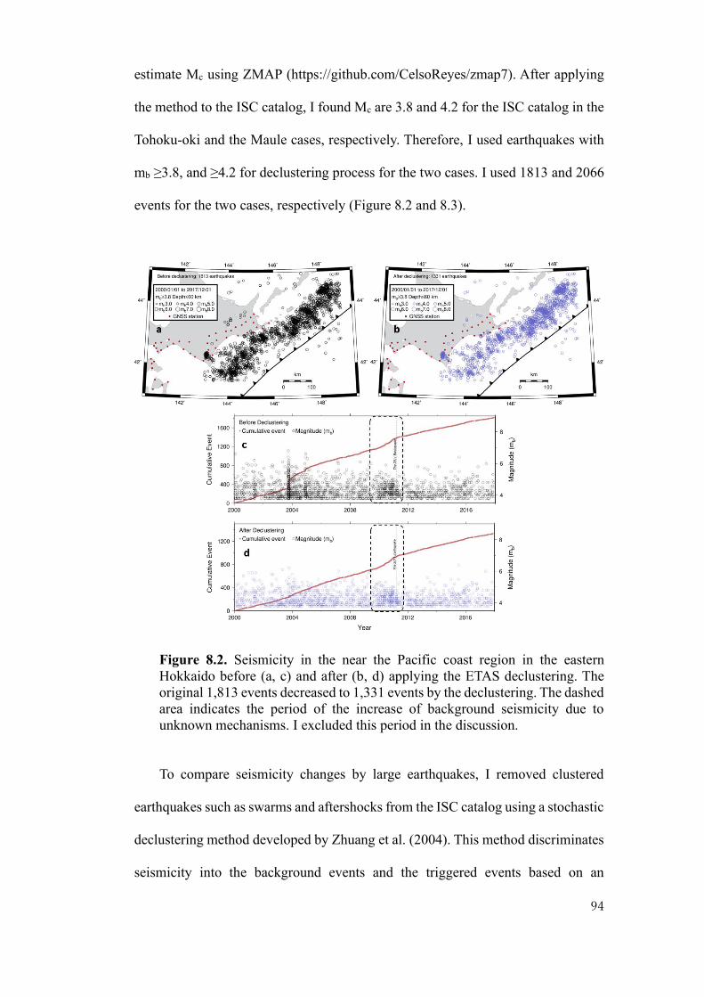
94

estimate Mc using ZMAP (https://github.com/CelsoReyes/zmap7). After applying

the method to the ISC catalog, I found Mc are 3.8 and 4.2 for the ISC catalog in the

Tohoku-oki and the Maule cases, respectively. Therefore, I used earthquakes with

mb ≥3.8, and ≥4.2 for declustering process for the two cases. I used 1813 and 2066

events for the two cases, respectively (Figure 8.2 and 8.3).

Figure 8.2. Seismicity in the near the Pacific coast region in the eastern

Hokkaido before (a, c) and after (b, d) applying the ETAS declustering. The

original 1,813 events decreased to 1,331 events by the declustering. The dashed

area indicates the period of the increase of background seismicity due to

unknown mechanisms. I excluded this period in the discussion.

To compare seismicity changes by large earthquakes, I removed clustered

earthquakes such as swarms and aftershocks from the ISC catalog using a stochastic

declustering method developed by Zhuang et al. (2004). This method discriminates

seismicity into the background events and the triggered events based on an

95

Epidemic-Type Aftershock Sequence (ETAS) model (Ogata, 1988). I used a

computer code for the space-time ETAS model and stochastic declustering from

http://bemlar.ism.ac.jp/zhuang/software. Parameters estimated from fitting the

ETAS models to the ISC catalog are listed in Table 8.1. After declustering process,

1,331 and 761 events remained as background events in the near east coast

Hokkaido and near the Pacific coast of central Chile (Figure 8.2 and 8.3),

respectively. I used these background events for further analyses.

Figure 8.3. Seismicity in the near Pacific coast of central Chile before (a, c)

and after (b, d) the application of the ETAS declustering. There are 2,066 events

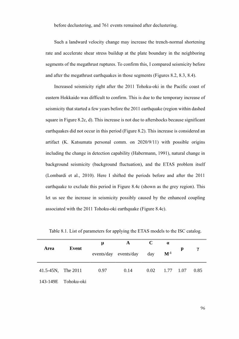
96

before declustering, and 761 events remained after declustering.

Such a landward velocity change may increase the trench-normal shortening

rate and accelerate shear stress buildup at the plate boundary in the neighboring

segments of the megathrust ruptures. To confirm this, I compared seismicity before

and after the megathrust earthquakes in those segments (Figures 8.2, 8.3, 8.4).

Increased seismicity right after the 2011 Tohoku-oki in the Pacific coast of

eastern Hokkaido was difficult to confirm. This is due to the temporary increase of

seismicity that started a few years before the 2011 earthquake (region within dashed

square in Figure 8.2c, d). This increase is not due to aftershocks because significant

earthquakes did not occur in this period (Figure 8.2). This increase is considered an

artifact (K. Katsumata personal comm. on 2020/9/11) with possible origins

including the change in detection capability (Habermann, 1991), natural change in

background seismicity (background fluctuation), and the ETAS problem itself

(Lombardi et al., 2010). Here I shifted the periods before and after the 2011

earthquake to exclude this period in Figure 8.4c (shown as the grey region). This

let us see the increase in seismicity possibly caused by the enhanced coupling

associated with the 2011 Tohoku-oki earthquake (Figure 8.4c).

Table 8.1. List of parameters for applying the ETAS models to the ISC catalog.

Area Event

µ

events/day

A

events/day

C

day

α

M-1

p γ

41.5-45N,

143-149E

The 2011

Tohoku-oki

0.97 0.14 0.02 1.77 1.07 0.85

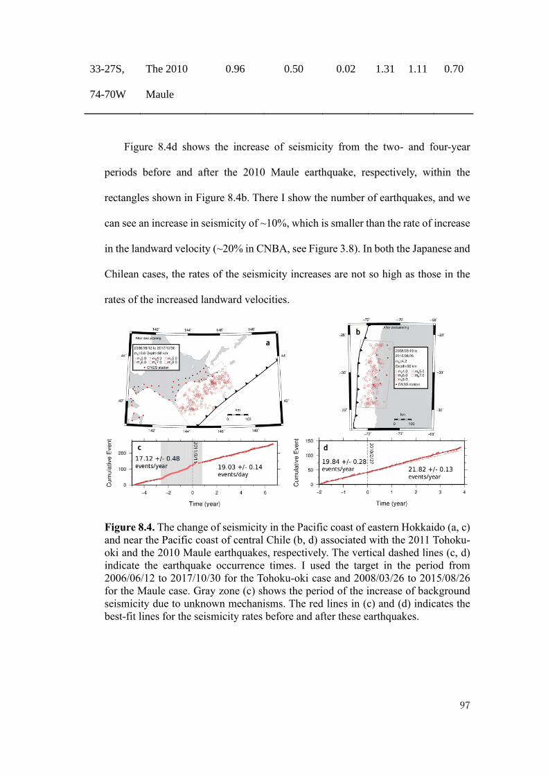
97

33-27S,

74-70W

The 2010

Maule

0.96 0.50 0.02 1.31 1.11 0.70

Figure 8.4d shows the increase of seismicity from the two- and four-year

periods before and after the 2010 Maule earthquake, respectively, within the

rectangles shown in Figure 8.4b. There I show the number of earthquakes, and we

can see an increase in seismicity of ~10%, which is smaller than the rate of increase

in the landward velocity (~20% in CNBA, see Figure 3.8). In both the Japanese and

Chilean cases, the rates of the seismicity increases are not so high as those in the

rates of the increased landward velocities.

Figure 8.4. The change of seismicity in the Pacific coast of eastern Hokkaido (a, c)

and near the Pacific coast of central Chile (b, d) associated with the 2011 Tohoku-

oki and the 2010 Maule earthquakes, respectively. The vertical dashed lines (c, d)

indicate the earthquake occurrence times. I used the target in the period from

2006/06/12 to 2017/10/30 for the Tohoku-oki case and 2008/03/26 to 2015/08/26

for the Maule case. Gray zone (c) shows the period of the increase of background

seismicity due to unknown mechanisms. The red lines in (c) and (d) indicates the

best-fit lines for the seismicity rates before and after these earthquakes.

98

Chapter 6: Conclusion

The concept of the seismic cycle develops quite dynamically through time. It

began as a simple model with a constant strain accumulation and regular

recurrences of interplate earthquakes. Subsequently, space geodetic observations

revealed the existence of transient postseismic processes such as afterslip and

viscous relaxation as an additional component in this cycle. Past researches further

added a brand-new stage following a massive earthquake in a subduction zone. This

new stage is characterized by the accelerated interseismic stain buildup in segment

adjacent along-strike to the ruptured segments.

I compiled GNSS data showing increased landward velocities that occurred in

segments adjacent along-strike to six recent megathrust earthquakes in four

different subduction zones (Figure 1.5). The results presented here confirmed

previous studies for the 2003 Tokachi-oki (Heki and Mitsui, 2013), the 2010 Maule

(Melnick et al., 2017), and the 2014 Iquique (Hoffmann et al., 2018) earthquakes. I

also updated the case of the 2011 Tohoku-oki earthquake, studied briefly in Heki

and Mitsui (2013), using GNSS data over a longer time span. I found similar

landward increase of velocity signatures for three more earthquakes in Sumatra,

Chile, and Mexico subduction zones.

From the three cases, i.e. the 2003 Tokachi-oki, the 2011 Tohoku-oki and the

2010 Maule earthquakes, where multiple GNSS stations were available from

various distances from the faults, I studied spatial extents of the phenomenon. There

I found that the landward velocity change extends along-strike to distances

comparable to the ruptured fault length (400-500 km) from the fault center (i.e.

99

extending by a half of the fault length beyond the fault edge) (Figure 4.1d).

Temporal decay was not clear suggesting much longer time constants of the

phenomenon than known postseismic processes such as afterslip and viscous

relaxation.

The velocity change showed a positive correlation with Mw and seems to scale

with the average slip. This is consistent with the hypothetical slab acceleration

model by Heki and Mitsui (2013) but does not rule out other possibilities. Such

increased landward velocity would enhance stress accumulation rate in adjacent

segments, encouraging future earthquakes in such segments, e.g. the eastern

Hokkaido.

In Chapter 5, I investigated the seismicity rate changes following the two largest

earthquakes showing the increased landward velocities. I used data from the ISC

bulletin and applied the ETAS declustering method to discriminate seismicity into

the background events and the triggered events. The background seismicity after

the 2011 Tohoku-oki in the Pacific coast of eastern Hokkaido increased from 17.1

± 0.5 events/year to 19.0 ± 0.1 events/year. In Chile, the background seismicity rate

increased from 19.8 ± 0.3 events/year to 21.8 ± 0.1 events/year after the 2010 Maule

earthquake. These results show a moderate increase in seismic activities. However,

the ratio of the increase to the original rate is not so high as those of the landward

velocity increases.

100

The contents of this thesis have been published in Tectonophysics:

Yuzariyadi, M., and Heki, K., 2021. Enhancement of interplate coupling in

adjacent segments after recent megathrust earthquakes. Tectonophysics, 801,

228719. https://doi.org/10.1016/j.tecto.2021.228719.

101

References

Abercrombie, R.E., Antolik, M. and G. Ekström., 2003. The June 2000 Mw7.9

earthquakes south of Sumatra: Deformation in the India-Australia Plate. J.

Geophys. Res. Solid Earth 108, ESE 6-1-ESE 6-16,

doi:10.1029/2001JB000674.

Abidin, H.Z., Susilo, S., Meilano, I., Subarya, C., Prijatna, K., Syafi’I, M.A.,

Hendrayana., Effendi, J., Sukmayadi, D., 2016. On the development and

implementation of a semi-dynamic datum for Indonesia. C. Rizos, P. Willis

(eds), IAG 150 Years, International Association of Geodesy Symposea 143, doi:

10.1007/1345_2015_83.

Anderson, D.L., 1975. Accelerated plate tectonics. Science, 187, 1077-1079

Ardika, M., Meilano, I., and Gunawan, E., 2015. Postseismic Deformation

Parameters of the 2010 M7.8 Mentawai, Indonesia, Earthquake Inferred from

Continous GPS observations. Asian J. earth Sci., 8(4): 127-133, doi:

10.3923/ajes.2015.127.133.

Argus, D.F., Gordon, R.G. and DeMets, C., 2011. Geologically current motion of

56 plates relative to the no-net-rotation reference frame, Geochem. Geophys.

Geosyst. 12, doi:10.1029/2011GC003751.

Atwater, T., and Stock, J.M., 1998. Pacific–North America plate tectonics of the

Neogene Southwestern United States: an update. International Geology

Review, 40 (5), 375–402.

Bird, P., Kagan, Y. Y., Jackson, D. D., Schoenberg, F. P. and Werner, M. J., 2009.

Linear and nonlinear relations between relative plate velocity and seismicity.

Bull. Seismol. Soc. Am. 99, 3097–3113, doi: 10.1785/0120090082.

Blewitt, G., Hammond, W. C., and Kreemer, C., 2018. Harnessing the GPS data

explosion for interdisciplinary science. EOS, 99, doi: 10.1029/2018EO104623.

Broerse, T. (2012): Megathrust Earthquakes: Study of Fault Slip and Stress

Relaxation Using Satellite Gravity Observations. PhD Thesis, Delft University

of Technology, ISBN 9789461862822

Bürgmann, R., Segall, P., Lisowski, M., and Svarc, J., 1997. Postseismic strain

following the 1989 Loma Prieta earthquake from GPS and Leveling

measurements. J. Geophys. Res., 102, B3, 4933-4955.

Cande, S.C., and Leslie, R.B., 1989. Late Cenozoic Tectonics of the Southern

Chile Trench. Journal of Geophysical Research Atmospheres, 91, B1, doi:

10.1029/JB091iB01p00471.

Choe, H., and Dyment, J., 2020. Fading magnetic anomalies, thermal structure

and earthquakes in the Japan Trench. Geology, 48, 278–282, doi:

10.1130/G46842.1.

Courboulex, F., Singh, S.K., Pacheco, J.F., and Ammon, C.J., 1997. The 1995

Colima-Jalisco, Mexico, earthquake (Mw 8): A study of rupture process.

Geophys. Res. Lett. 24(8): 1019-1022 doi:10.1029/97GL00945.

102

Curray, J. R., 1989. The Sunda Arc: A Model for Oblique Plate Convergence.

Netherlands Journal of Sea Research, 24 (2/3), 131-140.

Deal, M.M., and Nolet, G., 1999. Slab temperature and thickness from seismic

tomography2. Izu-Bonin, Japan, and Kuril subduction zones. J. Geophys. Res.

104(12) 28803-28812.

D’Acquisto, M., Herman, M., and Govers, R., 2020. On the cause of enhanced

landward motion of the overriding plate after a major subduction earthquake.

paper presented at the European Geophysical Union General Assembly, May.

4, 2020.

Einarsson, I., Hoechner, A., Wang, R., and Kusche, J., 2010. Gravity Changes Due

to the Sumatra-Andaman and Nias Earthquakes as Detected by the GRACE

Satellites: A Reexamination. Geophys. J. Int., 183, 733–747 doi:

10.1111/j.1365-246X.2010.04756.x.

Feng, L., Hill, E.M., Banerjee, P., Hermawan, I., Tsang, L.L.H., Natawidjaja, D.H.,

Suwargadi, B.W., and Sieh, K., 2015. A unified GPS-based earthquake catalog

for the Sumatran plate boundary between 2002 and 2013. J. Geophys. Res.,

120, 3566-3598, doi:10.1002/2014JB011661.

Fukahata, Y., and Matsu’ura, M., 2005. General expressions for internal

deformation fields due to a dislocation source in a multilayered elastic half-

space. Geophys. J. Int., 161, 507–521, doi: 10.1111/j.1365-246X.2005.02594.x.

Fukahata, Y., and Matsu’ura, M., 2006. Quasi-static internal deformation due to a

dislocation source in a multilayered elastic/viscoelastic half-space and an

equivalence theorem. Geophys. J. Int., 166, 418–434, doi: 10.1111/j.1365-

246X.2006.02921.x.

Fukao, Y., Obayashi, M., Nakakuki, T., et al., 2009. Stagnant Slab: A Review Annu.

Rev. Earth Planet. Sci., 37, 10.1–10.28, doi: 0.1146/annurev.earth.36.031207.

124224.

Gunawan, E., 2014. Comprehensive postseismic deformation model of the 2004

Sumatra-Andaman earthquake constrained by GPS data in northern Sumatra.

A dissertation for the degree of Doctor of Science Department of Earth and

Environmental Sciences, Graduate School of Environmental Studies, Nagoya

University.

Habermann, R.E., 1991.Seismicity rate variations and systematic changes in

magnitudes in teleseismic catalogs. Tectonophysics, 193, 4, 277-289, doi:

10.1016/0040-1951(91)90337-R.

Hafkenscheid, E., Buiter, S.J.H., Wortel, M.J.R., Spakman, W., and Bijwaard, H.,

2001. Modelling the seismic velocity structure beneath Indonesia: a

comparison with tomography. Tectonophysics 333, 35-46

Hamilton W., 1988. Plate tectonics and island arcs, Geol. Soc. Am. Bull., 100,

1503–1527.

Han, S.C., Sauber, J., Luthcke, S. B., Ji, C., and Pollitz, F. F., 2008. Implications of

postseismic gravity change following the great 2004 Sumatra-Andaman

earthquake from the regional harmonic analysis of GRACE intersatellite

tracking data. J. Geophys. Res., 113, B11413.

Hanifa, N.R., Sagiya, T., Kimata, F., Efendi, J., Abidin, H.Z., and Meilano, I.,

2014. Interplate coupling model off the southwestern coast of Java, Indonesia,

based on continuous GPS data in 2008-2010. Earth Planet. Sci. Lett. 401,

159-171, doi: 10.1016/j.epsl.2014.06.010.

103

Haridhi, H.A., Huang, B.S., Wen, K.L., Denzema, D., Prasetyo, R.A., and Lee, C.S.,

2018. A study of large earthquake sequences in the Sumatra subduction zone

and its possible implications. Terr. Atmos. Ocean. Sci., 29(6), 635-652, doi:

10.3319/TAO.2018.08.22.01.

Heki, K., and Mitsui, Y., 2013. Accelerated pacific plate subduction following

interplate thrust earthquakes at the Japan trench. Earth Planet. Sci. Lett., 363,

44–49, doi: 10.1016/j.epsl.2012.12.031.

Heki, K., Miyazaki, S. and Tsuji, H., 1997. Silent fault slip following an interplate

thrust earthquake at the Japan Trench. Nature, 386, 595-597.

Herring, T. A., King, R. W., Floyd, M. A., and McClusky S. C., 2018. Introduction

to GAMIT/GLOBK, Release 10.7. geoweb.mit.edu/gg/intro_GG.pdf.

Heuret, A., Conrad, C. P., Funiciello, F., Lallemand, S., and Sandri, L., 2012.

Relation between subduction megathrust earthquakes, trench sediment

thickness and upper plate strain. Geophys. Res. Lett. 39, L05304,

doi:10.1029/2011GL050712.

Hoffmann, F., Metzger, S., Moreno, M., Deng, Z., Sippl, C., Ortega-Culaciati, F.,

and Oncken, O., 2018. Characterizing afterslip and ground displacement rate

increase following the 2014 Iquique Pisagua Mw 8.1 earthquake, Northern

Chile. J. Geophys. Res. Solid Earth, 123, 4171–4192, doi:

org/10.1002/2017JB014970.

Husker. A., and Davis, P.M., 2009. Tomography and thermal state of the Cocos plate

subduction beneath Mexico City. J. Geophys. Res. 114, B04306,

doi:1029/2008JB006039

Ide, S., 2013. The proportionality between relative plate velocity and seismicity in

subduction zones. Nature Geosci. 6, 780-785, doi: 10.1038/NGEO1901.

Itoh, Y., and Nishimura, T., 2016. Characteristics of postseismic deformation

following the 2003 Tokachi-oki earthquake and estimation of the viscoelastic

structure in Hokkaido, northern Japan. Earth, Planets Space 68, 156, doi:

10.1186/s40623-016-0533-y.

Jónsson, S., Segall, P., Pedersen, R., and Björnsson, G., 2003. Post-earthquake

ground movements correlated to pore-pressure transients. Nature, 434, 179-183.

Kanamori, H., 1978. Quantification of earthquakes, Nature, 271, 411-414.

Kanamori, H., Jennings, P.C., Singh, S.K., and Astiz, L., 1993. Estimation of strong

ground motion in Mexico City expected for large earthquakes in the Guerrero

Seismic Gap. Bull. Seismol. Soc. Am. 83(3), 811-829.

Kelleher, J. A., 1972. Rupture zones of large South American earthquakes and some

predictions. J. Geophys. Res. 77(11), 2087–2103.

King, G. C. P., Stein, R.S., and Lin, J., 1994. Static stress changes and the triggering

of earthquakes, Bull. Seismol. Soc. Am., 84, 935-953.

Kiser, E., and Ishii, M., 2012. The March 11, 2011 Tohoku-oki earthquake and

cascading failure of the plate interface. Geophys. Res. Lett., 39, L00G25,

doi:10.1029/2012GL051170.

Klein, E., Fleitout,L., Vigny, C., and Garaud, J.D., 2016. Afterslip and viscoelastic

relaxation model inferred from the large-scale post-seismic deformation

following the 2010 Mw 8.8 Maule earthquake (Chile). Geophys. J. Int., 205,

1455–1472, doi: 10.1093/gji/ggw086.

Kodaira, S., Nakamura, Y., Yamamoto, Y., Obana, K., Fujie, G., No, T., Kaiho, Y.,

Sato, T., and Miura, S., 2017. Depth-varying structural characters in the rupture

104

zone of the 2011 Tohoku-oki earthquake. Geosphere; 13, 5,

doi:10.1130/GES01489.1.

Larsen, S., Reilinger, R., Neugebauer, H., and Strange, W., 1992. Global Positioning

System measurements of deformation associated with the 1987 Superstition

Hills earthquake: evidence for conjugate faulting. J. Geophys. Res., 97, B4,

4885-4902.

Li, S., Moreno, M., Bedford, J., Rosenau, M., and Oncken, O., 2015. Revisiting

viscoelastic effects on interseismic deformation and locking degree: A case

study of the Peru-North Chile subduction zone. J. Geophys. Res. 120, 4522–

4538, doi:10.1002/2015JB011903.

Lisowski, M., Prescott, W.H., Savage, J.C., and Johnston, M.J., 1990. Geodetic

estimate of coseismic slip during the 1989 Loma Prieta, California, earthquake.

Geophys. Res. Lett., 17(9) 1437-1440.

Lombardi, A.M., Cocco, M., and Marzocchi, W., 2010. On the increase of

background seismicity rate during the 1997-1998 Umbria-Marche, central

Italy, sequence: Apparent variation or fluid-driven triggering?. Bull. Seismol.

Soc. Am., 100, 3, 1138-1152, doi:10.1785/0120090077.

Loveless, J.P., 2017. Super-interseismic periods: Redifining earthquake recurrence.

Geophys. Res. Lett., 44, doi: 10.1002/2017GL072525.

Lubis, A.M., Hashima, A., and Sato, T., 2012. Analysis of afterslip distribution

following the 2007 September 12 southern Sumatra earthquake using

poroelastic and viscoelastic media. Geophys. J. Int., doi: 10.1093/gji/ggs020.

Manea, V.C., Manea, M., and Ferrari, L., 2013. Geodynamical perspective on the

subduction of Cocos and Rivera plates beneath Mexico and Central America.

Tectonophysics, doi: 10.1016/j.tecto.2012.12.039.

Marsan, D., and Enescu, B., 2012. Modeling the foreshock sequence prior to the

2011, MW9.0 Tohoku, Japan, earthquake. J. Geophys. Res., 117, B06316,

doi:10.1029/2011JB009039.

Materna, K., Bartlow, N., Wech, A., Williams, C., and Burgmann, R., 2019.

Dynamically Triggered Changes of Plate Interface Coupling in Southern

Cascadia. Geophys. Res. Lett. 46, 12890-12899,

doi:10.1029/2019GL084395.

Mavrommatis, A., Segall, P., and Johnson, K.M., 2014. A decadal-scale

deformation transient prior to the 2011 Mw 9.0 Tohoku-oki earthquake.

Geophys. Res. Lett., 41, 4486–4494, doi:10.1002/2014GL060139.

Melnick, D., Moreno, M., Quinteros, J., Baez, J.C., Deng, Z., Li, S., and Oncken,

O., 2017. The super-interseismic phase of the megathrust earthquake cycle in

Chile. Geophys. Res. Lett., 44, doi:10.1002/2016GL071845.

Metois, M., Socquet, A., Vigny, C., Carrizo, D., Peyrat, S., Delorme, A., Maureira,

E., Valderas-Bermejo M.-C., and Ortega I., 2013. Revisiting the North Chile

seismic gap segmentation using GPS-derived interseismic coupling. Geophys.

J. Int. doi: 10.1093/gji/ggt183.

Mignan, A., King, G., Bowman, D., Lacassin, R., and Dmowska, R., 2006. Seismic

activity in the Sumatra-Java region prior to the December 26, 2004. (Mw=9.0-

9.3) and March 28, 2005 (Mw=8.7) earthquake. Earth Planet. Sci. Lett. 244,

639-654, doi: 10.1016/j.epsl.2006.01.058.

Miyazaki, S., Segall, P., Fukuda, J., and Kato T., 2004. Space time distribution of

afterslip following the 2003 Tokachi-oki earthquake: Implications for

105

variations in fault zone frictional properties. Geophys. Res. Lett., 31, L06623,

doi:10.1029/2003GL019410.

Moreno, M., Melnick, D., Rosenau, M., Bolte, J., Klotz, J., Echtler, H., Baez, J.,

Bataille, K., Chen, J., Bevis, M., Hase, H., and Oncken, O., 2011.

Heterogeneous plate locking in the South–Central Chile subduction zone:

building up the next great earthquake. Earth Planet. Sci. Lett. 305, 413–424.

doi: 10.1016/j.epsl.2011.03.025.

Moreno, M., Melnick, D., Rosenau, M., Baez, J., Klotz, J., Oncken, O., Tassara, A.,

Chen, J., Bataille, K., Bevis, M., Socquet, A., Bolte, J., Vigny, C., Brooks, B.,

Ryder, I., Grund, V., Smalley, B., Carrizo, D., Bartsch, M., Hase, H., 2012.

Toward understanding tectonic control on the Mw 8.8 2010 Maule Chile

earthquake. Earth Planet. Sci. Lett. 321-322, 152-165, doi:

10.1016/j.espl.2012.01.006.

Muller, R. D., Sdrolias, M., Gaina, C., and Roest, W. R., 2008. Age, spreading

rates, and spreading asymmetry of the world's ocean crust. Geochemistry,

Geophysics, Geosystems, 9, Q04006., doi: 10.1029/2007GC001743.

Müller, R.D., Roest, W.R., Royer, J.Y., Gahagan, L.M., and Sclater, J.G., 1997.

Digital isochrons of the worlds ocean floor. J. geophys. Res., 102, B2, 3211-

3214. doi: 10.1029/96JB01781.

Nakagawa, H., Toyofuku, T., Kotani, K., Miyahara, B., Iwashita, C., Kawamoto, S.,

Hatanaka, Y., Munekane, H., Ishimoto, M., Yutsudo, T., Ishikura, N., Sugawara,

Y., 2009. Development and validation of GEONET new analysis strategy

(Version 4). J. Geogr. Surv. Inst. 118, 1–8, in Japanese.

Natawidjaja, D. H., Sieh, K., Chlieh, M., Galetzka, J., Suwargadi, B.W., Cheng, H.,

Edwards, R. L., Avouac, J‐P., and Ward, S. N., 2006. Source parameters of

the great Sumatran megathrust earthquakes of 1797 and 1833 inferred from

coral microatolls, J. Geophys. Res. 111, B06403, doi:10.1029/2005JB004025.

Niitsuma, N., 2004. Japan Trench and tectonics of the Japanese Island Arcs. The

Island Arc 13, 306–317.

Nur, A., Mavko, G., 1974. Postseismic viscoelastic rebound. Science 183, 204–206.

Ogata, Y., 1988. Statistical Models for Earthquake Occurrences and Residual

Analysis for Point Processes. Journal of the American Statistical Association,

83, 401. (Mar., 1988), pp. 9-27

Ozawa, S., Kaidzu, M., Murakami, M., Imakiire, T., Hanataka, Y., 2004. Coseismic

and postseismic crustal deformation after the Mw 8 Tokachi-oki earthquake in

Japan. Earth Planet Space, 56, 675-680.

Panet, I., Pollitz, F., Mikhailov, V., Diament, M., Banerjee, P., and Grijalva, K., 2010.

Upper mantle rheology from GRACE and GPS postseismic deformation after

the 2004 Sumatra–Andaman earthquake. Geochemical, Geophysics.

Geosystem. Vol 11, doi:10.1029/2009GC002905.

Peltzer, G., P. Rosen, F. Rogez, dan K. Hudnut., (1998): Poroelastic rebound along

the Landers 1992 earthquake surface rupture. Journal of Geophysics Research.,

103 (B12), 30131-30146.

Peng, Y., Zhou, S., Zhuang, J., and Shi, J., 2012. An approach to detect the

abnormal seismicity increase in Southwestern China triggered co-seismically

by 2004 Sumatra Mw 9.2 earthquake. Geophys. J. Int., 189, 1734–1740, doi:

10.1111/j.1365-246X.2012.05456.x.

Perfettini, H., Avouac, J.-P., Ruegg, J.C., 2005. Geodetic displacements and

106

aftershocks following the 2001 Mw=8.4 Peru earthquake: Implications for the

mechanics of the earthquake cycle along subduction zones. J. Geophys. Res.

110, B09404, doi:10.1029/2004JB003522.

Pesicek, J.D., Engdahl,E. R., Thurber, C. H., DeShon, H. R., and Lange D., 2012.

Mantle subducting slab structure in the region of the 2010 M8.8 Maule

earthquake (30–40◦S), Chile. Geophys. J. Int., doi: 10.1111/j.1365-

246X.2012.05624.x.

Pollitz, F. F., Bürgmann, R., and Banerjee, P., 2006. Post-seismic relaxation

following the great 2004 Sumatra-Andaman earthquake on a compressible self-

gravitating Earth. Geophys. J. Int., 167(1), 397-420.

Prawirodirdjo, L., Bock, Y., McCaffrey, R., Genrich, J., Calais, E., Stevens, C.,

Puntodewo, S.S.O., Subarya, C., Rais, J., Zwick, P., and Fauzi., 1997.

Geodetic observations of interseismic strain segmentation at the Sumatra

subduction zone. Geophys. Res. Lett., 24, 21, 2601-2604.

Prawirodirdjo, L., Bock, Y., Genrich, J. F., Puntodewo, S. S. O., Rais, J., Subarya,

C., and Sutisna, S., 2000. One century of tectonic deformation along the

Sumatran fault from triangulation and Global Positioning System surveys, J.

Geophys. Res., 105(28), 28, 343–28,361, doi:10.1029/ 2000JB900150.

Pritchard, M.E., Simons, M., Rosen P. A., Hensley, S., and Webb, F. H., 2002. Co-

seismic slip from the 1995 July 30 Mw = 8.1 Antofagasta, Chile, earthquake

as constrained by InSAR and GPS observations. Geophys. J. Int. 150, 362–

376, doi: 10.1046/j.1365-246X.2002.01661.x.

Ritsema, J., Lay, T., and Kanamori, H., 2012. The 2011 Tohoku Earthquake.

Elements, 8, 183–188, doi: 10.2113/gselements.8.3.183.

Ruff, L., and Kanamori, H., 1980. Seismicity and the subduction process. Phys.

Earth Planet. Inter. 23, 240–252.

Ryder, I., 2006. Elastic and Viscoelastic Modelling of Postseismic Motion and Fault

Structures. Doctoral Thesis. Departement of Earth Sciences, University of

Oxford.

Sagiya, T., 2004. A decade of GEONET: 1994-2003 –The continuous GPS

observation in Japan and its impact on earthquake studies–. Earth Planet and

Space, 56, xxix-xli.

Satake, K., Nishimura, Y., Putra, S.P., Gusman, A. R., Sunendar, H., Fujii, Y.,

Tanioka, Y., Latief, H., and Yulianto, E., 2012. Tsunami source of the 2010

Mentawai, Indonesia earthquake inferred from tsunami field survey and

waveform modeling. PAGEOPH 170, 1567-1582.

Sato, M., Ishikawa, T., Ujihara, N., Yoshida, S., Fujita, M., Mochizuki, M. and

Asada, A., 2011. Displacement above the hypocenter of the 2011 Tohoku-oki

earthquake, Science, 332, 1395.

Segou, M. And Parsons, M., 2018. Testing earthquake links in Mexico from 1978

to the 2017 M = 8.1 Chiapas and M = 7.1 Puebla shocks. Geophys. Res. Lett.,

45, 708–714, doi: 10.1002/2017GL076237.

Savage, J.C., Lisowski, M., Svarc, J.L., 1994. Postseismic deformation following

the 1989 (M = 7.1) Loma Prieta, California, earthquake. J. Geophys. Res., 99,

B7, 13757-17765.

Savage, J.C., and Svarc, J.L., 1997. Postseismic deformation associated with the

1992 Mω = 7.3 Landers earthquake, southern California. J. Geophys. Res., 102,

B4, 7565-7577.

107

Schurr, B., Asch, G., Rosenau, M., Wang, R., Oncken, O., Barrientos, S., Salazar,

P., and Vilotte, J. P., 2012. The 2007 M7.7 Tocopilla northern Chile earthquake

sequence: Implications for along-strike and downdip rupture segmentation and

megathrust frictional behavior. J. Geophys. Res. 117, B05305,

doi:10.1029/2011JB009030.

Scire. A., Zandt, G., Beck, S., Long, M., and Wagner, L., 2017. The deforming

Nazca slab in the mantle transition zone and lower mantle: Constraints from

teleseismic tomography on the deeply subducted slab between 6°S and 32°S.

Geosphere, 13, 3, 665-680, doi:10.1130/GES01436.1.

Schubert, G., Turcotte, D. L., Olson, P., 2001. Mantle Convection in the Earth and

Planets. Cambridge University Press.

Shao, Z., Zhan, W., Zhang, L., and Xu, J., 2016. Analysis of the far field Co-seismic

and Post-seismic responses caused by the 2011 Mw 9.0 Tohoku-Oki earthquake.

Pure Appl. Geophys., 173, 411-424, doi: 10.1007/s00024-015-1131-9.

Shen, Z. K., Jackson, D.D., Feng, Y., Cline, M., Kim, M., Fang, P., and Bock, Y.,

1994. Postseismic deformation following the Landers earthquake, California,

28 June 1992. Bull. Seismol. Soc. Am., 84, 3, 780-791.

Shinohara, M., et al.,2012. Precise aftershock distribution of the 2011 off the Pacific

coast of Tohoku Earthquake revealed by an ocean-bottom seismometer

network. Earth Planets Space, 64, 1137–1148, doi:10.5047/eps.2012.09.003.

Simons, W. J. F. et al., 2007. A decade of GPS in Southeast Asia: Resolving

Sundaland motion and boundaries. J. Geophys. Res. 112, B06420,

doi:10.1029/2005JB003868.

Singh, S. K., Comte, D., and Pardo, M. 1992. Background seismicity and strength

of coupling in the subduction zones. Bull. Seismol. Soc. Am. 82, 2114–2125.

Stern, R. J., 2002. Subduction zones. Rev. Geophys., 40(4), 1012,

doi:10.1029/2001RG000108.

Suito, H., and Freymueller, J. T., 2009. A viscoelastic and afterslip postseismic

deformation model for the 1964 Alaska earthquake. J. Geophys. Res.,Vol 114,

B11404, doi:10.1029/2008JB005954.

Sun, T., Wang, K., Iinuma, T., Hino, R., He, J., Fujimoto, H., Kido., M., Osada, Y.,

Miura, S., Ohta, Y., and Hu, Y., 2014. Prevalence of viscoelastic relaxation after

the 2011 Tohoku-oki earthquake. Nature, 514, doi:10.1038/nature13778.

Susilohadi, S., Gaedicke, C., and Djajadihardja, Y., 2009. Structures and

sedimentary deposition in the Sunda Strait, Indonesia. Tectonophys, 467(1),

55-71., doi: 10.1016/j.tecto.2008.12.015.

Tajima, F., Mori, J., and Kennet, B.L.N., 2013. A review of the 2011 Tohoku-oki

earthquake (Mw 9.0): Large-scale rupture across heterogeneous plate

coupling. Tectonophysics 586, 15-34, doi: 10.1016/j.tecto.2012.09.014.

Takahashi, H., and Kasahara, M., 2004. The 2003 Tokachi-oki earthquake, off

Southeastern Hokkaido, Japan. Journal of the Seismological Society of Japan,

57, 2, 115-130, doi: 10.4294/zisin1948.57.2_115.

Takano, T., 2011. Overview of the 2011 East Japan Earthquake and Tsunami

Disaster. The 2011 East Japan Earthquake Bulletin of the Tohoku

Geographical Association.

Tanioka, Y., et al., 2004. Tsunami run-up heights of the 2003 Tokachi-oki

earthquake. Earth Planets Space, 56, 359–365.

108

Tanioka, Y. and Katsumata, K., 2007. Tsunami generated by the 2004 Kushiro-oki

earthquake. Earth Planets Space, 59, e1-e3.

Thatcher, W., and Rundle, J. B., 1984. A viscoelastic coupling model for the cyclic

deformation due to periodically repeated earthquakes at subduction zones. J.

Geophys. Res., 89, 7631–7640.

Tsuji, H., Hatanaka, Y., Sagiya, T. And Hashimoto, M., 1995. Coseismic crustal

deformation from the 1994 Hokkaido-Toho-Oki earthquake monitored by a

nationwide continuous GPS arary in Japan. Geophys. Res. Lett., 22, 1669-

1672.

Uchida, N., and Matsuzawa, T., 2013. Pre- and postseismic slow slip surrounding

the 2011 Tohoku-oki earthquake rupture. Earth and Planetary Science Letters,

374, 81–91, doi: 10.1016/j.epsl.2013.05.021.

Uchida, N., Asano, Y., and Hasegawa, A., 2016. Acceleration of regional plate

subduction beneath Kanto, Japan, after the 2011 Tohoku-oki earthquake.

Geophys. Res. Lett., 43, 9002–9008, doi:10.1002/2016GL070298.

Uyeda, S., 1982. Subduction zones: An introduction to comparative subductology.

Tectonophys., 81, 133-159.

Uyeda, S., and Kanamori, H., 1979. Back-arc opening and the mode of

subduction. J. Geophys. Res. 84, 1049–1061.

Vigny, C., et al., 2011. The 2010 Mw 8.8 Maule megathrust earthquake of Central

Chile, monitored by GPS. Science 332, 1417-1421, doi:10.1126/

science.1204132.

Villegas-Lanza, J. C., Chlieh M., Cavalié O., Tavera H., Baby P., Chire-Chira J.,

and Nocquet J.-M., 2016. Active tectonics of Peru: Heterogeneous

interseismic coupling along the Nazca megathrust, rigid motion of the

Peruvian Sliver, and Subandean shortening accommodation. J. Geophys. Res.,

121, 7371–7394, doi:10.1002/2016JB013080.

Wang, K., 2007. In the Seismogenic Zone of Subduction Thrust Faults (eds Dixon,

T. H. & Moore, J. C.) 540–574. Columbia University Press.

Wang, K., Y. Hu, and J. He (2012), Deformation cycles of subduction earthquakes

in a viscoelastic Earth, Nature. 484, 327-332, doi:10.1038/nature11032.

Wiemer, S. and Wyss, M., 2000. Minimum Magnitude of Completeness in

Earthquake Catalogs: Examples from Alaska, the Western United States, and

Japan. Bull. Seismol. Soc. Am., 90, 4, 859–869.

Yamagiwa, S., Miyazaki, S., Hirahara, K., and Fukahata, Y., 2015. Afterslip and

viscoelastic relaxation following the 2011 Tohoku-oki earthquake (Mw9.0)

inferred from inland GPS and seafloor GPS Acoustic data. Geophys. Res. Lett.,

42, 66–73, doi:10.1002/2014GL061735.

Yáñez G., Ranero C.R., and Díaz J., 2001. Magnetic Anomaly interpretation

across the southern central Andes (32°–34°S): The role of the Juan Fernández

Ridge in the late Tertiary evolution of the margin. J. Geophys. Res., 106,

6325-6345.

Zhuang, J. O Ogata, Y., and Vere-Jones, D., 2004. Analyzing earthquake

clustering features by using stochastic reconstruction. J. Geophys. Res., 109,

B05301. doi:10.1029/2003JB002879.