comprehensive stormwater control measure (scm) hydrologic
TRANSCRIPT

Comprehensive Stormwater Control Measure (SCM) Hydrologic Performance Modeling
Preliminary SCM Performance Assessment as part of the NERRS Science Collaborative Project in Northern Ohio
Cardno JFNew
11/21/2014 This material is based on work supported by the National Oceanic and Atmospheric Association under Cooperative Agreement No. NA09NOS4190153 through the University of New Hampshire. Any opinions, findings, and conclusions or recommendations are those of the author and do not necessarily reflect those of the National Oceanic and Atmospheric Association or the University of New Hampshire.

Preliminary NERRS SC LID SCM Performance Model Study
1
PROJECT BACKGROUND
This project is led by the Old Woman Creek National Estuarine Research Reserve (OWC NERR) and the
Chagrin River Watershed Partners, Inc. (CRWP). The ultimate goal is to develop science-based tools to
help minimize the impact of stormwater on Ohio's coastal communities and Lake Erie. The project team
is using the Collaborative Learning method to work with municipal and consulting engineers,
stormwater utilities, developers, regulators, and watershed organizations to generate credible and
locally verified performance information about innovative stormwater controls. Based on these results,
the team will develop credits and incentives to encourage the use of the most effective systems. This
work was funded by the National Oceanic and Atmospheric Administration through the National
Estuarine Research Reserve System Science Collaborative Program (NERRS SC) administered by the
University of New Hampshire.

Preliminary NERRS SC LID SCM Performance Model Study
2
EXECUTIVE SUMMARY .................................................................................................................................. 4
1. BACKGROUND ....................................................................................................................................... 6
1.1 NERRS Science Collaborative Project .................................................................................................. 7
1.1. 1 Modeling Project ........................................................................................................................ 8
2. METHODOLOGY .................................................................................................................................... 8
2.1. Unit Base Models .......................................................................................................................... 9
2.2. SCM Design Variable Sensitivity Analyses ................................................................................... 14
2.3. Annual, Continuous SCM Simulations ......................................................................................... 15
2.4. Analysis of SCM Attainment of Water Quality Volume and Critical Storm Event Peak Flow
Control .................................................................................................................................................... 16
3. RESULTS............................................................................................................................................... 18
3.1. SWMM Software Issues .............................................................................................................. 18
3.2. Single Event – Base Design and Sensitivity Analysis Results ....................................................... 19
3.2.1. Type 1 & Type 2 SCMs: Storage + Infiltration + (for Type 1 only) Optional Sump .............. 24
3.2.2. Type 3 SCMs: Flow-Through ............................................................................................... 26
3.2.3. Type 4 SCM: Soil Renovation .............................................................................................. 26
3.2.4. Type 5 SCM: Green Roof ..................................................................................................... 27
3.3. SCM Results for Continuous, Annual Hydrograph Runs ............................................................. 28
4. CONCLUSIONS AND RECOMMENDATIONS ......................................................................................... 28
4.1. Conclusions ................................................................................................................................. 29
4.2. Recommendations ...................................................................................................................... 30
4.2.1. Recommendations for Development of a WQv Credit ....................................................... 31
4.2.2. Recommendations for Development of a Critical Storm Event Credit ............................... 32
4.2.3. Recommendations for a Soil Renovation Credit System .................................................... 32
5. REFERENCES ........................................................................................................................................ 34
Table of Tables
Table 1. Subcatchment Properties – Existing Conditions ........................................................................... 10
Table 2. Green-Ampt Parameters ............................................................................................................... 11
Table 3. Summary of SCM Variables and Their Associated Ranges ............................................................ 14
Table 4. Calculation of Critical Storm Events for Three Pre-Development Conditions .............................. 17

Preliminary NERRS SC LID SCM Performance Model Study
3
Table of Figures
Figure 1. Flow Chart of Individual-Event SCM Analyses ............................................................................. 13
Figure 2. Average Annual Daily Temperature and Total Annual Rainfall for the Cleveland-Hopkins Airport
from 1950-2012 (NOAA) ............................................................................................................................. 16
Figure 3. Color-Coded Bioretention Volume Reduction Results for HSG C Soils at a 5% DAR ................... 20
Figure 4. SCM Types and Their Functional Differences (each SCM type and their functional processes are
exemplified by one example SCM schematic. All SCM schematics can be found in the Appendix)........... 21
APPENDICES
A. SCM Input Tables
B. SCM Single-Event Results Tables
C. SCM Continuous, Annual Results Tables

Preliminary NERRS SC LID SCM Performance Model Study
4
EXECUTIVE SUMMARY This technical memorandum summarizes the goals and objectives, model analyses, assumptions,
shortcomings, results and recommendations for the preliminary modeling work of the National
Estuarine Research Reserve System Science Collaborative (NERRS SC)-funded stormwater monitoring
and modeling project in northern Ohio. This modeling effort entailed more than 30,000 dynamic
hydrologic and hydraulic model runs for individual design storm events and for continuous, annual
stormwater control measure (SCM) performance simulations. These analyses have helped lay the
foundation for a SCM design/crediting system to be developed by ODNR for inclusion in the Ohio
Rainwater and Land Development Manual.
The objectives of the NERRS SC modeling work include:
• Build believable and defensible models of Low Impact Development (LID) SCMs to assess volume
reduction and peak discharge attenuation capabilities. The models need to reasonably account
for Ohio stormwater standards, site conditions and climate.
• Develop and apply a wide-ranging sensitivity analysis to determine the relative importance of
site conditions and SCM design variables to volume and peak discharge reductions using both
individual storm event models and continuous, year-long simulations.
• Assess the capability of LID SCMs, across the range of applied site and design variables, to meet
State of Ohio water quality volume (WQv) and critical storm event control guidelines.
• Suggest procedures for development of a crediting system that will help provide designers,
owners, regulators, etc., a convenient way to design and take credit for the use of LID SCMs.
Ultimately, this work, in combination with the monitoring and follow-on modeling, will be used to:
• Appropriately credit LID SCMs for volume reduction and peak discharge attenuation
• Refine SCM design specifications where needed
• Develop design and accounting guidance and tools consistent with specifications, research
results, and models
The USEPA Storm Water Management Model (SWMM, v.5.0) was the primary model used in this
analysis. The selection of climatic data and model parameterization for nine SCMs – bioretention,
permeable pavement, dry detention, underground storage, green roofs, infiltration trenches, filter
strips, swales, and soil renovation – was a collaborative effort between the Ohio Department of Natural
Resources (ODNR) Division of Soil and Water Resources, Chagrin River Watershed Partners, Inc. (CRWP)
and Cardno JFNew, the consultant on the project. A Collaborative Learning Group (CLG) of stormwater
engineers, regulators, and professionals convened for the NERRS SC project also provided input on
modeling parameters and results. Two general sets of model runs were performed: 1) single storm

Preliminary NERRS SC LID SCM Performance Model Study
5
event analyses for ten synthetic rainfall events from 0.25-inch depth up to 3.5-inches; and 2)
continuous, annual runs for representative dry, average and wet years using data from the Cleveland
Hopkins Airport National Oceanic and Atmospheric Administration (NOAA) weather station.
SWMM was used to quantify pre- and post-development runoff and the effectiveness of LID SCMs for
managing post-development site hydrology and meeting stormwater management requirements. A set
of base pre-development model scenarios was created, one for each of the Natural Resource
Conservation Service (NRCS) hydrologic soil groups - A, B, C and D. As the basis for the post-
development analysis, half of the drainage area was “developed” as impervious area and the site
modeled to determine runoff volume and peak flow rates with no stormwater controls in place. The
LID SCMs were applied to the developed watershed, and reductions in runoff volume and peak flow rate
estimated.
In general, we found most modeling results were consistent with expectations and field data. While the
models have not yet been calibrated with field monitoring data, some initial comparisons of model-
estimated and data-calculated volume reductions appear to show a reasonable correspondence.
The ratio of SCM area to total drainage area (the Drainage Area Ratio or DAR) is the most influential
variable for generating inflows, while permanent volume losses are most dependent on underlying soil
type. Design variables such as sump depth (also known as Internal Water Storage or IWS), depth of
engineered media, etc., variably impact performance depending on the underlying soil type, the DAR,
and type of SCM. Generally the more functional attributes, such as surface ponding, subsurface storage,
IWS (or “sump”), etc., an SCM possesses, the better its hydrologic performance. Although we did not
quantify the impact, actual performance of SCMs will vary based on antecedent moisture conditions. If
pore space or ponding volume is already occupied when a follow-on event occurs, the SCM performance
will suffer. All individual event analyses were run with initial soil moisture at field capacity.
We believe this analysis helps lay the foundation for an LID SCM crediting system. While the Ohio
Rainwater and Land Development Manual provides guidance for meeting the state WQv requirement,
there is no explicit guidance to credit runoff volume reduction provided by LID SCMs. This work shows
clear relationships between DAR, underlying soil types, and performance. It also provides estimates of
volume reductions as a function of design variables. The performance results permit direct evaluation of
the LID system’s ability to meet the WQv (0.75-inch event) and a simple way to credit that volume
reduction toward reducing the critical storm event recurrence interval.
The conservative approach to SCM volume reduction credits assumes that credits are additive whether
multiple SCMs on a site are installed in parallel or in series. In reality, when SCMs are applied in series
actual volume reductions may exceed reductions calculated for each SCM separately; designers will still
need to route runoff through their systems as part of a permit application process. Routing may
demonstrate peak flow reductions provided by LID SCMs exceed those attributable to volume reduction
alone. Additional research to understand the systematic differences between SCMs in parallel and in
series is needed.

Preliminary NERRS SC LID SCM Performance Model Study
6
Before a crediting system can be finalized, model performance needs to be tested against monitoring
data. North Carolina State University Stormwater Engineering Group (NCSU) performed hydrologic and
water quality monitoring of several newly installed bioretention and permeable pavement in northern
Ohio SCMs for the NERRS SC project. This monitoring will provide detailed data sets for SCM model
calibration and validation.
In addition, results from the continuous, annual event runs should be used to pro-rate projected single
storm event performance with adjustments that account for performance variation as a function of
antecedent moisture conditions. Volume credits can then be calculated as active SCM storage volume
plus some discounted infiltration volume. Peak flow credits will require additional analysis in order to
connect SCM sizing, selection, and placement with reasonable and justifiable performance.
Project results suggest another line of research and potentially another crediting mechanism. Volume
reductions are highly correlated to underlying soil hydrology. Despite knowing that quantifying soil
hydrology involves a variety of factors, many of which cannot be controlled during or following the land
conversion process, the stormwater industry has over-simplified soil hydrology with the assignment of
curve numbers based on hydrologic soil group (HSG-A, B, C, D).
Unfortunately, there is a dearth of information on how to appropriately maintain, recover or even
characterize soil hydrologic function in our urban landscapes. As a result, modeled volume reductions
driven by SCM surficial soil quality – soil renovation, filter strips, grass swales, dry detention basins –
carry a higher level of uncertainty than those based on capture of a stored volume (bioretention,
permeable pavement, underground detention, infiltration trench). Additional research to augment our
understanding of how to preserve inherent hydrologic function, use soil renovation (compost
amendments, tillage, etc.), plant selection and vegetation management to enhance soil quality, or
measure or model soil hydrology resulting from typical or innovative site development practices, will aid
in development of appropriate credits and reward the conservation or development of more
ecologically functional landscapes.
1. BACKGROUND Stormwater runoff from impervious surfaces severely impacts Ohio's coastal communities and
environments. It erodes streams, overloads drainage systems and wastewater treatment facilities, and
increases flooding, causing damage to property and infrastructure. Increased runoff also impairs water
quality and degrades habitats, and heightens the risk of waterborne diseases. The severity of these
impacts has increased with the number of heavy storms in Ohio, which are up 31 percent over the past
50 years according to the U.S. Global Change Research Program (Pryor, et al., 2009; Pryor, et al., 2014).
This has been reflected in widespread and frequent flooding in Lake Erie counties over the last five
years.
Ohio Environmental Protection Agency (Ohio EPA) stormwater regulations require new development to
treat the first 3/4-inch of rain, also known as the "water quality volume" (WQv). Redeveloped sites must
treat 20% of the WQv or reduce impervious cover by 20%. Most communities have peak discharge

Preliminary NERRS SC LID SCM Performance Model Study
7
requirements for infrequent recurrence interval events (typically the 1 – 100 year return period)
targeted at flood control. Most new developments meet these requirements with traditional "end-of-
pipe" ponds that do not reduce the volume of stormwater runoff, allowing further degradation of Ohio’s
streams (Ohio EPA, 2007; Ohio EPA, 2011).
Low impact development (LID) attempts to address these problems by integrating the functions
inherent to natural landscapes into site design and stormwater systems. This methodology includes
open space preservation, clustered development, rainwater reuse, and distributed SCMs (in contrast to
centralized, end-of-pipe solutions). Ohio communities and design engineers have asked for design
criteria, credits, and other incentives to catalyze a shift to LID approaches.
1.1 NERRS Science Collaborative Project The primary goal of the “Implementing Credits and Incentives for Innovative Stormwater Management”
project, funded through the National Estuarine Research Reserve System (NERRS) Science Collaborative
program, is to develop science-based tools to help minimize the impact of stormwater on Ohio's coastal
communities and Lake Erie. This project, spearheaded by the Old Woman Creek National Estuarine
Research Reserve (OWC NERR) and the Chagrin River Watershed Partners, Inc. (CRWP), will: (1) provide
guidance and tools to help engineers, reviewers, and permitting agencies determine whether LID
stormwater systems are appropriate for their sites to meet state and local requirements; and (2)
demonstrate the design, construction, performance, and maintenance of these stormwater practices in
local soils and climate. The project team is using a collaborative learning approach to engage a group of
interested experts for input and feedback throughout this project and to ensure the developed tools and
trainings are useful to the intended users. The project’s collaborative learning group (CLG) - comprised
of stormwater engineers, regulators, educators, stormwater utility managers, and watershed
organizations - has provided iterative guidance and feedback to the project team on the design,
construction, and monitoring processes of six SCM demonstration sites. The collaborative learning
process has enabled group members to share a broad range of knowledge, concerns, and ideas for
addressing complex stormwater challenges in northern Ohio.
Project partners and Collaborative Learning Group members include:
1. National Oceanic and Atmospheric Administration (NOAA) 2. Chagrin River Watershed Partners, Inc. (CRWP) 3. Old Woman Creek National Estuarine Research Reserve (OWC-NERR) 4. Ohio Department of Natural Resources, Division of Soil and Water Resources (ODNR-DSWR) 5. Erie Soil and Water Conservation District (Erie SWCD) 6. Firelands Coastal Tributaries 7. Ohio Department of Natural Resources, Division of Wildlife (ODNR-DOW) 8. Ohio Environmental Protection Agency (Ohio EPA) 9. GPD Group 10. CT Consultants 11. City of Aurora 12. Northeast Ohio Regional Sewer District (NEORSD) 13. Perkins Township, Erie County

Preliminary NERRS SC LID SCM Performance Model Study
8
14. Erie County Engineers Office 15. John Hancock & Associates 16. City of Sandusky 17. Forest City Land Group 18. Village of Kirtland Hills 19. Orange Village 20. Willoughby Hills 21. Pepper Pike 22. Ursuline College 23. Holden Arboretum 24. North Carolina State University Stormwater Engineering Group (NCSU)
25. Chagrin Valley Engineering
26. Stephen Hovansek and Associates
27. Cardno JFNew
1.1. 1 Modeling Project The modeling portion of the NERRS project included four main tasks: 1) develop base (“default”) unit-
scale SCM models for individual storm event analysis of SCMs; 2) perform a sensitivity analysis of SCM
design parameter impacts on runoff reductions; 3) perform an analysis of unit-scale SCMs, both base
and selected sensitivity analysis model runs, for average, wet, and dry continuous annual hydrographs;
and 4) develop site models for quantification, evaluation, and comparison of SCM performance for
runoff volume reduction, peak discharge control, and flow duration. Task 4 is a stand-alone task and will
be reported in a separate document.
USEPA SWMM v5 was used for all the modeling efforts. As part of future NERRS SC project work, some
of these models will be calibrated to field data being collected by NCSU on several sites in northern
Ohio. NCSU also will simulate bioretention and permeable pavement in DRAINMOD, a model typically
used to design and predict the impact of drain tiles on groundwater in agricultural fields. Work done at
NCSU (Brown, et.al., 2013) has already suggested DRAINMOD may be better suited than SWMM for
estimating the performance of SCMs outfitted with underdrains.
2. METHODOLOGY The analysis mirrored standard engineering practice for analyzing stormwater impacts for a “green field”
development site by estimating runoff for 1) undeveloped conditions, 2) developed conditions without
SCMs, and 3) developed conditions with SCMs. This comparative analysis allows the engineer/designer
to estimate the volume and peak flow reduction requirements and develop initial SCM design
parameters for their site. Each SCM was modeled over a range of sizes (as a fraction of total drainage
area) for a range of rainfall events including single events and annual, continuous rainfall data runs.
Individual SCM design parameters, such as ponding height, sump depth, etc., were varied between
model runs. Volume and peak flow reductions were estimated and where applicable compared to Ohio
Rainwater and Land Development Manual requirements.

Preliminary NERRS SC LID SCM Performance Model Study
9
Development of model inputs was a collaborative effort between the Ohio Department of Natural
Resources, Division of Soil and Water Resources (ODNR-DSWR) and Cardno JFNew with input from the
entire NERRS team, including the CLG and NCSU. SCM design variables were compiled from the Ohio
Rainwater and Land Development Manual (ODNR, 2006), the Michigan Low Impact Development
Manual (SEMCOG, 2008), professional experience, and a collection of data from research (Dierks, 2013;
Dierks, 2014; Fassman-Beck, et al., 2013; Toronto and Region Conservation, 2008; University of Guelph,
2013 and Van Seters, et al., 2006). Model inputs for the base cases and the design variable sensitivity
analyses can be found in Appendix A, attached.
2.1. Unit Base Models The unit scale modeling assumed a one-acre watershed for all scenarios, except dry detention. Standard
engineering design for dry detention, usually designed as a centralized, regional SCM, typically utilizes a
larger contributing watershed. Therefore, the dry detention contributing watershed area was set at ten
acres. Three pre-development land use scenarios were modeled - row-crop agriculture, pasture and
forest - with each scenario run using generalized soil properties representing the four Natural Resources
Conservation Service (NRCS) hydrologic soil classifications – A (well-drained), B (moderately drained), C
(poorly drained) and D (very poorly drained) – for a total of twelve pre-development scenarios.
Infiltration and runoff from pervious areas were simulated using the Green-Ampt equation in order to
explicitly represent dynamic soil water storage. Post-developed conditions assumed half the watershed
was converted to impervious surface and the other half to turf grass. The pre-development and post-
development conditions were used to calculate the recurrence interval, and thus the size of the critical
storm event for peak discharge control per Ohio DNR guidance.
Model inputs for the pre-developed watershed scenarios are shown in Tables 1 and 2 below. Watershed
width defines the shape of the watershed. Watershed area divided by the width gives the flow path
length across the watershed. Watershed slope (% slope) is the average fall divided by flow path length
(expressed as a percentage) across the watershed area. Mannings n is a friction factor, or measure of
surface roughness, used to estimate the velocity of sheet flow across the ground surface. The higher the
n-value the greater the energy loss and the longer it takes water to flow across the watershed. The n-
value increased in magnitude from agriculture to pasture to forest per USEPA SWMM guidance (Huber,
et al., 1988). The surface storage parameter Dstore defines the micro-topographical interception storage
created by small, surficial depressions that fill with water before runoff occurs.

Preliminary NERRS SC LID SCM Performance Model Study
10
Table 1. Subcatchment Properties – Existing Conditions
Model Property
Land Use
Agriculture Pasture Forest
Area (acres) 1 1 1
Width (feet) 200 200 200
% Slope 2 2 2
% Impervious area 0 0 0
Sheet flow Mannings n 0.1 0.3 0.6
Surface Storage (Dstore) (inches) 0.05 0.05 0.075
Infiltration Parameters Green-Ampt Green-Ampt Green-Ampt
The Green-Ampt infiltration equation, used to simulate water movement through the unsaturated soil
column above groundwater (also referred to as the vadose zone), relies on three soil parameters: 1) the
initial moisture deficit, 2) the matric suction (or suction head) and 3) hydraulic conductivity. The initial
moisture deficit is the pore void space available to temporarily store water. The matric suction or
suction head can be thought of as the suction (negative pressure) necessary to break the force of
attraction between pore water and soil particles. At saturation the matric suction equals zero – water
flows via gravity. As the volumetric water content in the pores decreases, the matric suction, expressed
as a negative pressure, increases; i.e., it gets harder to “pull” the water away from the soil. Conductivity
is saturated hydraulic conductivity, the rate at which water moves through saturated soil.
The selected values for the HSG A, B, C and D soils used in the model represent the average values for
sandy loam, loam, sandy clay loam, and silty clay, respectively, as estimated from thousands of soils
samples collected by the United States Department of Agriculture (USDA), almost exclusively from
agricultural land (Rawls, et al., 1982). It is worth noting there are no sandy clay loam soils in Ohio, but
the predominant silt loam, silty clay loam and clay loam soils found in Ohio can be adequately
represented by the generic C or D soil characteristics used in this study.
The Green-Ampt parameters used in the model are summarized in Table 2 below. The matric suction
and initial moisture deficit values assume the soil is at field capacity. Field capacity is the volume of
water left in a soil after all the water that can drain via gravity has drained away. SWMM dynamically
tracks the changes in soil moisture and infiltration over the course of a simulation. Any water that
cannot infiltrate because the soil is saturated and cannot be accommodated by micro-topographical
storage (Dstore) becomes runoff.

Preliminary NERRS SC LID SCM Performance Model Study
11
Table 2. Green-Ampt Parameters
For “developed” watersheds, turf grass was given an n-value of 0.2 and a surface storage of 0.05. The
developed watersheds were then “treated” with one of nine SCMs using the SWMM LID tool where
possible. The SWMM LID tool has built-in sub-routines to store and infiltrate runoff for bioretention,
porous pavers, vegetated swales, infiltration trenches, green roofs, rain gardens and rain barrels. The
built-in LID tool was used to simulate SCMs except for underground detention, dry detention and soil
renovation. Soil renovation was simulated as a change in post-development pervious area infiltration
rates. Underground detention and dry detention were simulated as storage units with bottom seepage
in the hydraulic routing portion of SWMM.
Unit-scale SCMs analyzed for this project included:
1. Bioretention 2. Permeable pavement 3. Underground detention/retention
a. Alt 1: water quality volume storage and outlet, with excess inflow discarded from the system as runoff
b. Alt 2: storage and outlets for both water quality volume and peak discharge control 4. Infiltration trench 5. Dry detention
a. Alt 1: water quality volume storage and outlet, with all excess inflow above depth of water quality volume leaving as surface runoff
b. Alt 2: storage and outlets for both water quality volume and peak discharge control 6. Water quality swale (with infiltration) 7. Vegetated/grassed filter strip 8. Soil renovation 9. Green roof
With the exceptions of permeable pavement, green roof, and soil renovation SCMs, models for each
SCM type covered a range of drainage area ratios (DARs) - the ratio of SCM area to total contributing
area – of 1%, 2%, 5%, 10% and 25%. For permeable pavement, the 1% and 2% DARs were not modeled
since they far exceed recommended hydrologic loading; instead a 50% DAR was added (Smith, 2011).
Likewise for green roofs, the unreasonably small DARs of 1%, 2% and 5% were dropped and 50%, 75%
and 100% scenarios were added. For soil renovation, only the 50% DAR was analyzed. For soil
renovation the impervious area runoff was routed over the pervious area.
Each modeling scenario involved many factors: the combination of pervious and impervious area,
various DARs for each SCM, the four different HSGs, and ten separate rainfall events – 0.25-inch, 0.5-
A B C D
Suction Head (in) 2.41 3.5 8.6 11.5
Conductivity (in/hr) 2.35 0.52 0.12 0.04
Initial Deficit (fraction) 0.312 0.193 0.143 0.092
Soil Hydrologic ClassModel Properites

Preliminary NERRS SC LID SCM Performance Model Study
12
inch, 0.75-inch, 1.0-inch, 1.25-inch, 1.5-inch, 2.0-inch, 2.5-inch, 3.0-inch, and 3.5-inch. Rainfall was
modeled by distributing it over three hours using the Huff 2nd quartile distribution (Huff and Angel,
1992). Evapotranspiration was set to zero for all single event runs. The assumption here is during a rain
event, with relative humidity near 100%, there is little gradient to drive water back into the atmosphere.
To the extent this may not be the case in reality, this assumption errs on the conservative side. A
flowchart to exemplify how this simulation process works is shown in Figure 1.

Figure 1. Flow Chart of Individual-Event SCM Analyses
1-ac Undeveloped
Agriculture Pasture Forest
Development
0.5-ac imp0.5-ac grass
2% 5% 10%1% 25%
B C DA
B C DA
PPT0.25-in0.50-in0.75-in1.00-in1.25-in1.50-in2.00-in2.50-in3.00-in3.50-in
Underlying soil
LEGEND
Un-developed
Developed

Preliminary NERRS SC LID SCM Performance Model Study
14
2.2. SCM Design Variable Sensitivity Analyses Following development of the unit base models, a sensitivity analysis was devised to vary SCM design
parameters within a set of ranges an engineer or designer might consider. The idea was to identify
which SCM design parameters were most responsible for runoff volume reduction and peak flow
mitigation. Table 3 below summarizes the range of variables applied to the set of SCMs. A full set of
parameters and base case for each SCM are detailed in Appendix A. Note, due to the similarity of the
results for permeable pavements and infiltration trenches, no sensitivity runs were performed for the
infiltration trench.
Table 3. Summary of SCM Variables and Their Associated Ranges
*For grassed swales, the depth variable is maximum potential flow depth, not ponding depth. Mix =
typical green roof media. LS = loamy sand. SL = sandy loam
Design Variables Bio
rete
nti
on
Po
rou
s P
aver
s
Dry
Det
enti
on
Un
der
gro
un
d D
eten
tio
n
Gre
en R
oo
f
Gra
ssed
Sw
ale
Filt
er S
trip
So
il R
eno
vati
on
Drainage Area Ratio (%) 1-25 5-50 1-25 1-25 10-100 1-25 1-25 50
HSGs A-D A-D A-D A,C A,C A-D A-D
Surface Ponding Depth (in) 6-18 0 1-22 0 24* 0.05 0.05
Subsurface Storage Height (in) 18-30 12-36 0 30 2-4 0 0 0
Drain Offset (in) 3-18 0-6 0 0-12 0
Media Thickness (in) 24-48 2-4
Media Composition LS, LS/SL, SL Mix , LS/SL
Pavement Permeability (in/hr) 10-1000
Vegetative Fraction (%) 5 5 0-5
Surface Roughness (n value) 0 0.012 0.2 0.05-0.41 0.12-0.36 0.2
Slope (%) 0 2 0.5 0.5-2 1-5 2
Side Slope (H:V) 3:1-5:1
Outlet Diameter (in) 1.3-3.1 2-4
Underdrain coeff (unitless) Varies Varies Varies
Hydraulic Conductivity (in/hr)Based on
media
Based on
Media 0.04-20.47

Preliminary NERRS SC LID SCM Performance Model Study
15
2.3. Annual, Continuous SCM Simulations The model results necessary to assess the impact of antecedent moisture conditions on the
performance of SCMs were created by running continuous, year-long simulations of both the base and
selected design parameter sensitivity cases. We compiled three continuous rainfall and temperature
data sets from the 62-year data record at Cleveland-Hopkins Airport: a dry year, 1963, with 18.63 inches
of total precipitation; an average year, 1979, with 37.95 inches; and a wet year, 2011, with 65.32 inches
(Figure 2).
The continuous, annual runs calculated daily ET within SWMM using the built-in Hargreaves equation.
The Hargreaves method is based on temperature and a correction factor for the amount of solar
radiation reaching the earth. This correction factor is based on the difference between the minimum
and maximum recorded temperatures for a day. The main energy source that drives ET is solar radiation
and the amount of solar radiation reaching the ground is mediated by cloud cover. The assumption is
under clear skies the atmosphere is transparent to solar radiation and the maximum temperature is
high, while night temperatures are low due to outgoing longwave radiation. Under cloudy skies less
radiation reaches the earth, so the maximum temperature is lower and night temperatures are relatively
higher as clouds limit outgoing longform radiation. Shahidan, et al. (2012) noted that because at least
80% of reference potential evapotranspiration can be explained by temperature and solar radiation and
the difference in temperature over a day is related to humidity and cloudiness, this method, while
approximate, provides a reasonable estimate of daily ET.
It is worth noting the Cleveland Hopkins average annual temperature and total rainfall data exhibit a
consistent upward trend for both data sets over the period of record. Although we did not explicitly
develop “climate change” model scenarios, the 2011 continuous model run represented the largest total
annual rainfall over the entire data record from the airport. In work yet to be completed, the NERRS SC
project will use precipitation data based on moderate and severe climate change scenarios for mid-
century (2050s) to simulate SCM performance under future climate conditions in SWMM and
DRAINMOD to evaluate climate change adaptation benefits of LID stormwater controls. Those data
have been provided by Drs. Fu and Hathaway of University of Tennessee/Oak Ridge National Laboratory.

Preliminary NERRS SC LID SCM Performance Model Study
16
Figure 2. Average Annual Daily Temperature and Total Annual Rainfall for the Cleveland-Hopkins Airport from 1950-2012 (NOAA-NCDC)
2.4. Analysis of SCM Attainment of Water Quality Volume and Critical Storm
Event Peak Flow Control Development in Ohio routinely is subject to the following two post-construction stormwater
management requirements:
1. State level requirement to capture and provide extended detention of the water quality volume
(WQv), the runoff from an 0.75-inch precipitation event (Ohio EPA, 2013). This requirement is
set by Ohio NPDES permits and is calculated as:
WQv = C*P*A/12
WQv = water quality volume (ac-ft)
C = runoff coefficient
P = precipitation (0.75-in)
A= area draining to BMP
For 0.5 acre impervious, assume C = 0.95 and A = 0.5 acre 31,293ftft0.059ac(0.5ac)/12*(0.75in)*(0.95)WQv
Add 20% for sediment storage:
31,552ft1.2*31,293ftWQv
46
47
48
49
50
51
52
53
54
55
56
0
10
20
30
40
50
60
70
1950 1960 1970 1980 1990 2000 2010
Mea
n T
emp
. (F)
Rai
nfa
ll (I
nch
es)
Cleveland-Hopkins International Airport
Average Rainfall Rainfall Mean Temp 5-yr Mov. Avg (PPT) 5 per. Mov. Avg. (Mean Temp)

Preliminary NERRS SC LID SCM Performance Model Study
17
2. Local peak discharge (sometimes called flood control) regulations; many Ohio communities have
adopted the Critical Storm Method (ODNR, 1980, 2006) for setting peak discharge requirements.
Calculate Critical Storm Event – ODNR (1980, 2006)
a. Assumed agriculture/pasture/forest pre-development area is converted to 50%
impervious and 50% turf grass (except for green roofs)
b. Must meet pre-development peak flow for critical event and all more frequent events
c. 1-yr, 2-yr, 5-yr, 10-yr, 25-yr, 50-yr, 100-yr
The Critical Storm Method (CSM) developed by ODNR (1980) sets standards for stormwater detention
based on the percent increase of runoff volume from the 1-year, 24-hour rainfall event for conversion
from undeveloped land to post-developed conditions. As the percentage increase from pre- to post-
development runoff volume gets larger, the recurrence interval for the event (the “critical storm”) that
must be captured and released at the 1-year pre-development discharge also gets larger. As would be
expected, increasing the impervious area on a development site will result in a bigger increase in post-
development runoff volume, a larger critical event size and hence a higher standard for runoff
detention.
Though the 1-year, 24-hour rainfall event was not explicitly modeled as part of this study, we felt the
modeled runoff volume from the 2.0” rainfall depth adequately represented this event; the depth of the
1-year, 24-hour rainfall event in northern Ohio generally falls between 1.9” and 2.2” (NOAA Atlas 14).
Table 4 summarizes the calculations to determine the critical storm.
Table 4. Calculation of Critical Storm Events for Three Pre-Development Conditions
1-yr Pre-Developed Runoff (cf)
Post-Dev 1-yr
Runoff (cf)
Runoff Increase (beyond 1-yr event predeveloped
condition)
HSG
Critical Storm Recurrence Interval
Forest Pasture Ag Forest Pasture Ag
Forest Pasture Ag
0 0 0 3556 > 500% > 500% > 500%
A 100-yr 100-yr
100-yr
141 235 420 3767 > 500% > 500% > 500%
B 100-yr 100-yr
100-yr
2093 2481 2840 4980 138% 101% 75%
C 25-yr 25-yr
10-yr
4028 4387 4708 5911 47% 35% 26%
D 5-yr 5-yr 5-yr
When determining the critical storm event, many communities require the pre- and post-development
runoff volumes from the 1-year, 24-hour event be calculated using the NRCS curve number method
(CN). Analysis conducted subsequent to the SWMM modeling reported here allowed comparison of
SWMM and CN runoff volume predictions, highlighting consistencies and differences in prediction of
how much stormwater is abstracted by impervious areas, open space, surface storage, etc. Those
comparisons will be considered when further analyzing SCM volume reductions, and developing credits

Preliminary NERRS SC LID SCM Performance Model Study
18
and guidance, to be applied to the Critical Storm Method. However, these are beyond the scope of this
study.
3. RESULTS The modeling outcomes can be divided into three groups based on our confidence in the results and
their utility to the overall goals of the project. The first group consists of information invested with a
high degree of confidence in its veracity and utility for informing stormwater design and regulatory
guidance. These results are characterized by conformance with expectations and performance data
from other studies and therefore should be useful for the development of stormwater design/regulatory
guidance. This report will focus primarily on the discussion and explication of this first group of results.
The second group is characterized by either confounding results or results that lack sufficient outside
verification. Thus, confidence in the veracity and usefulness of the data is somewhat compromised.
These results may or may not be a fault of the modeling technique or assumptions; may be a problem
endemic to the model software; or simply may currently lack sufficient external verification to draw
useful conclusions. This group of results warrants further investigation.
The third group of results is characterized by software issues, in which the model output blatantly
diverges from expectations. This issue appears to be traceable to a problem with the representation or
algorithm used to model the hydrologic processes. Discussion of the software issues will follow first and
then the discussion of the more useful results below.
3.1. SWMM Software Issues In general the SWMM LID tool results (on a mass-balance basis) appear adequate for the purposes of
this exercise. However, we did find three software issues that deserve mention: 1) the underdrain
simulation routine, 2) underdrain offset from SCM bottom and 3) swale side slopes.
The first software issue was the apparent misrepresentation of underdrains in SWMM. The control of
the outflow rate in the underdrain was set by an equation resembling the standard orifice equation,
with a flow coefficient and flow exponent. But the equation given in the manual did not appear to be
dimensionally consistent. SWMM model guidance for determining this coefficient appeared to be
flawed. Using the SWMM guidance, outflow rates were many times higher than the rates we have
observed from field monitoring data. We found it more reasonable to adjust the flow coefficient
downward to produce target underdrain outflow rates based on monitoring data from other studies
(Dierks, 2013; Toronto and Region Conservation, 2008; University of Guelph, 2013 and Van Seters, et al.,
2006).
Another issue encountered in the SWMM LID control was model representation versus real world
expectations for abstraction (temporary storage and subsequent exfiltration) of water when the
underdrain invert was set exactly at the bottom of the SCM. SWMM assumes water will immediately
leave the practice through the drain as soon as the water level reaches the drain invert, resulting in zero
or near zero infiltration when the modeled drain invert is placed at the bottom of the SCM. In reality,
the excavated bottom of the practice – especially if scarified to enhance exfiltration – will provide some

Preliminary NERRS SC LID SCM Performance Model Study
19
small level of storage as well as a relatively rough, hydraulically inefficient lateral pathway to the drain.
In our opinion, using a zero offset in SWMM overestimates the amount of water lost through the
underdrain and underestimates the amount of water infiltrating through the bottom of the SCM. Using a
small non-zero outlet offset above the bottom of the SCM substantially improved performance. The
results below for SCMs with underdrains located at the bottom of the practice reflect SWMM models in
which the underdrain invert was placed 0.01 ft above the bottom of the practice.
For the swale side slopes, increasing swale side slopes decreased velocity through the section. This is
contrary to reality. Increasing side slopes creates a more hydraulically efficient open channel section.
Increased hydraulic efficiency means water moves more quickly through the channel. This is an inherent
problem with the model. We should note that since we started this work a new version of SWMM (5.1)
has been released. We have not tested the new model swale sub-routine since using the previous
version.
3.2. Single Event – Based Design and Sensitivity Analysis Results In order to efficiently present the immense amount of information produced, we developed a color-
coded interpretive display of the SCM volume and peak reduction performance. This display lays out
thousands of data points at one time (bioretention volume and peak flow reduction graphs alone
represent 4,800 data points) for a quick comparative survey of all the results. This graphical
representation amalgamates the data into six performance categories based on percent volume or peak
flow reduction from the developed watershed scenarios. These categories, and an example of their
application to a set of volume reduction estimates for bioretention with underlying HSG C soils at a 5%
DAR, are shown in Figure 3 below.
Figure 3 shows this particular bioretention cell infiltrated more than 95% of the WQv (0.75”) event when
(1) the base design was modified to include a media thickness of 48 inches, (2) the media was loamy
sand, or (3) the underdrain offset was equal to or greater than 12 inches. One can also see performance
was somewhat sensitive to all of the particular design variables investigated here; that is, changing the
surface ponding, media thickness and type, and underdrain offset design variables all had an effect on
performance.
Lastly, much of the post-modeling analysis to determine individual SCM capabilities to meet peak flow
mitigation and volume reduction goals focused on C and D soils because most of northern Ohio has HSG
C and D soils and these are the most challenging soils over which to implement LID stormwater controls.

Preliminary NERRS SC LID SCM Performance Model Study
20
Figure 3. Color-Coded Bioretention Volume Reduction Results for HSG C Soils at a 5% DAR
*LS = loamy sand, SL=sandy loam
We divided the SCMs into five general types based on their functional characteristics:
Type 1 ) storage + infiltration + optional elevated outlet (sump): bioretention, permeable
pavements, underground detention/retention, and infiltration trench
Type 2) storage + infiltration (no sump): dry detention
Type 3) flow-through or conveyances (little to no storage and limited infiltration): grass swale
and filter strips
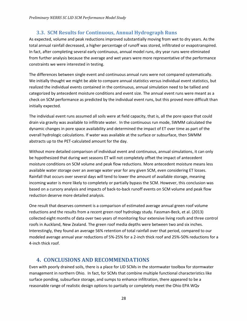
Type 4) source control: soil renovation
Type 5) SCMs with limited storage and no infiltration as a permanent loss: green roofs.
The differences in functional characteristics between these groups are exemplified in the SCM
schematics in Figure 4 below.
6 12 18 24 48 LS LS/SL SL 18 / 3 21 / 6 24 / 12 30 / 18
0.25
0.5
0.75
1.0
1.25
1.5
2.0
2.5
3.0
3.5
Precip
Surface Ponding
Depth (in)
Soil Thickness
(in)
Soil Type (porosity, field capacity,
wilting point, conductivity,
conductivity slope, suction head)
Storage Height / Underdrain
Offset (in)
Eve
nt
Size
(in
)

Preliminary NERRS SC LID SCM Performance Model Study
21
ET (for annual runs only)
Run-in Run-out
Infiltration
Surface Storage
Figure 4. SCM Types and Their Functional Differences (each SCM type and their functional processes are exemplified by one example SCM schematic. All SCM schematics can be found in the Appendix)
ET (for annual runs only) Outflow
Infiltration
Berm height
Inflow
Type 1 SCM: Storage + Infiltration + Optional Sump Bioretention Permeable Pavement Underground Storage Infiltration Trench
Type 3 SCM: Flow Through: Little to No Storage + Limited Infiltration Grass Swale Filter Strip
Surface Storage
ET (for annual runs only)
Infiltration
Staged Outflow
Run-in
Type 2 SCM: Storage + Infiltration + No Sump Dry Detention
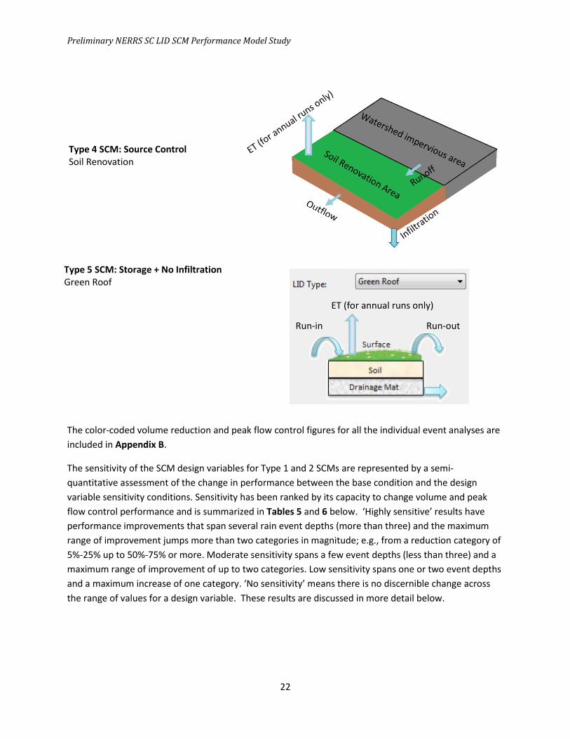
Preliminary NERRS SC LID SCM Performance Model Study
22
ET (for annual runs only)
Run-out Run-in
The color-coded volume reduction and peak flow control figures for all the individual event analyses are
included in Appendix B.
The sensitivity of the SCM design variables for Type 1 and 2 SCMs are represented by a semi-
quantitative assessment of the change in performance between the base condition and the design
variable sensitivity conditions. Sensitivity has been ranked by its capacity to change volume and peak
flow control performance and is summarized in Tables 5 and 6 below. ‘Highly sensitive’ results have
performance improvements that span several rain event depths (more than three) and the maximum
range of improvement jumps more than two categories in magnitude; e.g., from a reduction category of
5%-25% up to 50%-75% or more. Moderate sensitivity spans a few event depths (less than three) and a
maximum range of improvement of up to two categories. Low sensitivity spans one or two event depths
and a maximum increase of one category. ‘No sensitivity’ means there is no discernible change across
the range of values for a design variable. These results are discussed in more detail below.
Type 5 SCM: Storage + No Infiltration Green Roof
Type 4 SCM: Source Control Soil Renovation

Preliminary NERRS SC LID SCM Performance Model Study
23
Table 5. Sensitivity of Volume Reduction Results to SCM Design Parameters for Type 1 and 2 SCMs
(1=highly sensitive; 2=moderate; 3=low; 4= not sensitive; -1 = degradation of performance)
Table 6. Sensitivity of Peak Flow Reduction Results to SCM Design Parameters for Type 1 and 2 SCMs
(1=highly sensitive; 2=moderate; 3=low; 4= not sensitive; -1 = degradation of performance)
A B C D A B C D A B C D A B C D
Surface Ponding Depth (in) 1 1 2 3 2 2
Subsurface Storage Height (in) 4 4 4 4 3
Drain Offset (in) 1 1 1 1 1 1
Media Thickness (in) 4 4 1 2
Media Composition (in) 2 2 2 2
Pavement Permeability (in/hr) 4 4 4 4
Outlet Diameter (in) -1 -1
4 4 1 1
Design Variables
Bio
rete
nti
on
Po
rou
s P
aver
s
Dry
Det
enti
on
Un
der
gro
un
d
Det
enti
on
A B C D A B C D A B C D A B C D
Surface Ponding Depth (in) 1 1 2 3 2 2
Subsurface Storage Height (in) 4 4 4 4 1
Drain Offset (in) 1 1 1 1 1 1
Media Thickness (in) 4 4 3 4
Media Composition (in) 3 3 2 2
Pavement Permeability (in/hr) 3 3 3 3
Outlet Diameter (in) -1 -1
Design Variables
Bio
rete
nti
on
Po
rou
s P
aver
s
Dry
Det
enti
on
Un
der
gro
un
d
Det
enti
on
4 4 3 3

Preliminary NERRS SC LID SCM Performance Model Study
24
3.2.1. Type 1 & Type 2 SCMs: Storage + Infiltration + (for Type 1 only) Optional Sump
Table 7 summarizes volume reduction in terms of the WQv event (0.75” ppt) for all SCMs and all soil
classes.
SCM hydrologic performance was highly dependent on DAR and underlying soils, but also reflected the
number of functional characteristics, total depth of storage (ponding + subsurface storage), and sump
depth (raised outlet). The Type 1 and 2 SCMs with storage, infiltration and sumps produced the best
volume and peak flow reductions. Type 1 and 2 SCMs provided retention time for water to be lost via
infiltration and evapotranspiration, regardless of whether the storage was aboveground or below.
Bioretention with a sump exhibited the best volume and peak flow control performance overall.
Pervious pavements and underground detention outfitted with at least a 6-inch sump (orifice offset 6-
inches above the bottom) met the WQv through infiltration.
Permeable pavements, underground storage and bioretention were the three most versatile SCMs.
Permeable pavements offered versatility because they blended gray and green infrastructure.
Permeable paving can be strategically used in a spatially extensive manner as part of the hardscape –
parking lots and low-use roads and driveways – AND provided excellent hydrologic benefits. Similarly,
underground detention provided extensive hydrologic benefits while not consuming valuable
aboveground space. Bioretention offered versatility by possessing the greatest number of functional
characteristics – both above-ground and below-ground detention to provide time for infiltration and ET
of temporarily stored water, and the use of an optional sump to increase infiltration and ET.
Bioretention volume reduction was most sensitive to ponding depths for A and B soils and sump depth
for C and D soils. Bioretention located in C and D soils was also fairly sensitive to media thickness. The
effect of surface ponding depth on A and B soils diminished as the DAR increased. The effect of ponding
depth was almost absent by the time the DAR reached 10% and was zero by 25%. At low DARs (1%-5%),
additional surface ponding helped improve performance with A, B, and C soils but did not help for D
soils because as soon as the sump filled, any additional water was lost out the underdrain due to low
exfiltration rates.
For peak flow reduction with bioretention, all HSG cases were most sensitive to ponding depth, with C
and D soils also moderately sensitive to media composition. Across all HSGs as the DAR increased, the
smaller event peak flows get reduced more than 95%, so the increased storage with additional ponding
and media depth became less relevant for these small event sizes. For larger events storage depths still
mattered.

Preliminary NERRS SC LID SCM Performance Model Study
25
Table 7. Comparison of SCM Performance to Ohio EPA Water Quality Volume (WQv)
Notes: Blue with no text = infiltrated WQv under all scenarios, blue with text = infiltrated WQv with designs indicated, red = WQv not infiltrated. All scenarios run without ET losses. Dry detention Alt. 2 run for A and C soils only.
HSG
DAR (%) 2 5 10 25 50 2 5 10 25 50
Bioretention Ponding > 12" Not Run Not Run
Porous Pavers Not Run 6" sump Not Run 6" sump
Underground Storage Not Run Not Run Not Run Not Run Not Run sump >3" sump >0 Not Run
Dry Detention Alt 2 Not Run Not Run
Grass Swales Not Run Not Run Not Run Not Run Not Run Not Run
Filter Strips Not Run Not Run
Infiltration Trenches Not Run Not Run Not Run Not Run Not Run Not Run Not Run Not Run Not Run Not Run
Green Roofs
Soil Renovation Not Run Not Run Not Run Not Run >base infil Not Run Not Run Not Run Not Run >base infil
A B
HSG
DAR (%) 2 5 10 25 50 2 5 10 25 50
Bioretention
48" soil, LS or
>12" sumpNot Run
30" storage &
18" sumpNot Run
Porous Pavers Not RunAll but no
sumpNot Run
All but no
sump
Underground Storage Sump > 3" sump >0 Not Run Not Run Not Run Not Run Not Run Not Run
Dry Detention* Alt 2 Not Run Not Run
Grass Swales Not Run Not Run Not Run Not Run Not Run Not Run
Filter Strips Not Run Not Run
Infiltration Trenches Not Run Not Run
Green Roofs
Soil Renovation Not Run Not Run Not Run Not Run > high infil Not Run Not Run Not Run Not Run > max infil
C D

Preliminary NERRS SC LID SCM Performance Model Study
26
The other Type 1 SCMs - permeable pavements, infiltration trenches and underground detention - were
most sensitive to raised underdrains. This was consistent with observed behavior and intuition. Water
stored below the underdrain had a longer residence time in the SCM and consequently more potential
to infiltrate or evapotranspire. As expected, permeable pavements were relatively insensitive to the
depth of the underground storage alone. The difference in travel time between the 12-inch and 24-inch
aggregate depths in the model was insignificant so the impact on peak discharge was minimal, and
volume reduction was not affected at all. However, as the IWS zone thickness increased, both runoff
volumes and peak flows were reduced. Flow control added to the underdrain – in this case an orifice
with a smaller diameter – allows further management of peak discharge. With added aggregate depth
and flow rate control, it may be possible to totally meet peak discharge requirements with permeable
pavement.
Pavement permeability did not appear to affect performance of permeable pavement systems. The
lower limit of paver permeability was set at 10 inches/hour, a reasonable infiltration rate for a partially
clogged paver surface. This lower infiltration rate still was fast enough to drain runoff without negatively
affecting volume and peak flow reduction. This was not surprising since the mostly clogged paver
infiltration rate is 4, 19, 83 and 250 times faster than the model infiltration rates for underlying A, B, C
and D soils respectively. The underlying soils will have more of an impact on permeable pavement
system performance than partially clogged pavements as long as the DAR is greater than 33% and the
paver surface infiltration rate is > 10 inches/hour.
Dry detention appeared to be the SCM most sensitive to underlying HSG for volume control. The DAR
thresholds for fully infiltrating the WQv for A and B soils are 5% and 25%, whereas C soils and D soils can
only infiltrate up to 90% and 67% of the WQv at the 25% DAR, respectively. These volume reduction
outcomes carry over to peak discharge results, as the volume reduction benefits on C and D soils are not
significant enough to affect peak discharge for the 2-inch and larger events targeted by peak discharge
control requirements, whereas exfiltration from dry basins on HSG A and B soils may be significant.
3.2.2. Type 3 SCMs: Flow-Through or Conveyance
Type 3 SCMs are flow-through SCMs: grassed swales and filter strips. These SCMs possess fewer
functional characteristics. Grassed swales and filter strips slow and filter stormwater as shallow flow
moves through the grass. Neither practice detains stormwater, limiting opportunity for infiltration or
evapotranspiration. However, it was possible to improve their respective modeled performance by
slowing the rate of water movement through the SCM. In the case of grassed swales and filter strips,
decreasing slope and/or increasing vegetation density (and therefore roughness) effectively slowed the
water down and improved both volume and peak flow control performance. Decreasing swale side
slopes will also help in this regard, though likely not much; however, what appears to be inaccurate
representation of swale side slopes in SWMM prevented this analysis. Grass swales at 25% DARs and
filter strips at 10% and 25% DARs on A soils can infiltrate the WQv.
3.2.3. Type 4 SCM: Soil Renovation
Soil renovation as a source control is a unique SCM. Only a 50% DAR scenario for each HSG was
modeled. At infiltration rates indicative of natural landscapes, soil renovation showed the capacity to

Preliminary NERRS SC LID SCM Performance Model Study
27
capture the WQv and significantly reduce peak discharge, even on D soils. By renovating an existing soil,
whether by soil amendments or by planting deep-rooting plants, the water holding and infiltration
capacities increase. There is a growing body of literature that these impacts can be significant (Selbig
and Balster, 2010; University of Minnesota, 2011, Dierks, 2014). The research showed on average,
across all soil types, infiltration capacities increased between two and four times between cultivated
landscapes – row crops, active pasture and turf grass - and restored or native landscapes. Infiltration
rates increased up to ten and twenty times from cultivated to restored/native landscapes were
observed.
Research into “Urban Soil Husbandry” and “Suburban Subsoiling” has shown potential to reclaim the
runoff abstraction potential of our disturbed soils. Schwartz (2012) has been working with chisel plowing
and deep-tilling in combination with compost amendment to decompact urban and suburban soils. As
shown by Balousek (2003), chisel-plowing and deep tilling reduced runoff from silty soils during the 2002
growing season by 36% - 53% and, when compost was added, by 74% to 91%.
Soil renovation could simply entail exclusion of typical site development practices. Clear-cutting,
clearing and grubbing, and indiscriminately compacting to homogenize the development envelope is
unnecessary and destroys soil structure.
This SCM shows great promise because it has several linked benefits that accrue from its application,
particularly by implementing it as part of a native planting project. These benefits include stormwater
control, carbon sequestration, heat island mitigation, native habitat for pollinators, etc. It also shows
promise as a way to renovate and/or improve the performance of other SCMs, particularly dry
detention, filter strips, and grassed swales.
However, the benefits of a planted SCM tend to be time-dependent, on the scale of a few to many years
after planting, and there is still a great deal of uncertainty about how to predict benefits in advance of
performing the soil renovation. There is a need to investigate and learn how to credit this kind of
practice in the future.
3.2.4. Type 5 SCM: Green Roof
For green roofs, short of increasing the total green roof area, increasing the depth of the planting media
was the number one change in this analysis that improved both volume and peak flow control. Fassman-
Beck, et al. (2013) also recommended lengthening the flow path and the use of “drainage-retarding”
materials in the drainage layer. These recommendations were not tested in this analysis.
Without the capacity to infiltrate water into underlying soils, green roofs have only ET as the permanent
loss route. This limits the use of this SCM to meet the WQv or reduce the critical storm event size. The
green roof SCM reduced the WQv event less than 5% for 10% roof coverage and between 50% and 75%
for 100% roof coverage. By comparison Fassman-Beck, et al. (2013) measured green roof rainfall
retention of between 20% and 95% for rainfall near the WQv event (0.75-inches).
Preliminary NERRS SC LID SCM Performance Model Study
28
3.3. SCM Results for Continuous, Annual Hydrograph Runs As expected, volume and peak reductions improved substantially moving from wet to dry years. As the
total annual rainfall decreased, a higher percentage of runoff was stored, infiltrated or evapotranspired.
In fact, after completing several early continuous, annual model runs, dry year runs were eliminated
from further analysis because the average and wet years were more representative of the performance
constraints we were interested in testing.
The differences between single event and continuous annual runs were not compared systematically.
We initially thought we might be able to compare annual statistics versus individual event statistics, but
realized the individual events contained in the continuous, annual simulation need to be tallied and
categorized by antecedent moisture conditions and event size. The annual event runs were meant as a
check on SCM performance as predicted by the individual event runs, but this proved more difficult than
initially expected.
The individual event runs assumed all soils were at field capacity, that is, all the pore space that could
drain via gravity was available to infiltrate water. In the continuous run mode, SWMM calculated the
dynamic changes in pore space availability and determined the impact of ET over time as part of the
overall hydrologic calculations. If water was available at the surface or subsurface, then SWMM
abstracts up to the PET-calculated amount for the day.
Without more detailed comparison of individual event and continuous, annual simulations, it can only
be hypothesized that during wet seasons ET will not completely offset the impact of antecedent
moisture conditions on SCM volume and peak flow reductions. More antecedent moisture means less
available water storage over an average water year for any given SCM, even considering ET losses.
Rainfall that occurs over several days will tend to lower the amount of available storage, meaning
incoming water is more likely to completely or partially bypass the SCM. However, this conclusion was
based on a cursory analysis and impacts of back-to-back runoff events on SCM volume and peak flow
reduction deserve more detailed analysis.
One result that deserves comment is a comparison of estimated average annual green roof volume
reductions and the results from a recent green roof hydrology study. Fassman-Beck, et al. (2013)
collected eight months of data over two years of monitoring four extensive living roofs and three control
roofs in Auckland, New Zealand. The green roof media depths were between two and six inches.
Interestingly, they found an average 56% retention of total rainfall over that period, compared to our
modeled average annual year reductions of 5%-25% for a 2-inch thick roof and 25%-50% reductions for a
4-inch thick roof.
4. CONCLUSIONS AND RECOMMENDATIONS Even with poorly drained soils, there is a place for LID SCMs in the stormwater toolbox for stormwater
management in northern Ohio. In fact, for SCMs that combine multiple functional characteristics like
surface ponding, subsurface storage, and sumps to enhance infiltration, there appeared to be a
reasonable range of realistic design options to partially or completely meet the Ohio EPA WQv

Preliminary NERRS SC LID SCM Performance Model Study
29
requirement through infiltration and evapotranspiration. These volume reductions may help to reduce
the critical storm event and meet other local stormwater management requirements.
While this study managed to produce more than 30,000 model runs, not all the results were analyzed
exhaustively. We did not spend much time analyzing the year-long, continuous simulations. Before
developing a crediting system for LID SCMs, we believe the continuous simulations deserve additional
analysis. For instance, if a crediting system counts above and below ground storage, should any
allowance be made for antecedent moisture conditions? If so, how would adjustments to below ground
storage be made to account for antecedent moisture?
Another aspect of stormwater management not included in this study is the impact of winter conditions
– snow, ice and ground freezing. While it is appropriate to be concerned about this aspect of
performance, winter typically does not generate a lot of runoff. Spring thaw has a greater impact on
SCM hydrologic performance. However, there is work that shows freezing and thawing are complicated
and spatially varied processes. For example, Davidson, et al. (2008) found three out of four bioretention
cells continued to infiltrate runoff during three winter monitoring seasons in Minnesota, while the
fourth cell was limited primarily by tight soils.
Drainage area ratio (DAR) and the underlying soil are key criteria when selecting SCMs and considering
design options. DAR is a simple criterion that should provide designers a tool for preliminarily sizing their
SCMs. The importance of soils to modeled SCM performance reinforces the importance of knowing a
site’s soils and soil properties. As a corollary, this work also emphasizes the value that can accrue from
managing soil ecological resources in a manner that enhances their hydrologic properties.
4.1. Conclusions
1. SCM performance was most sensitive to DAR and underlying soil types. They were the primary
drivers of SCM sizing to meet runoff reduction goals. The crediting system should start from
allowable or recommended DARs, as a function of the type of SCM, and underlying soil type.
2. Sumps or IWS zones improve SCM performance for all infiltrating SCMs even over the tightest
of soils. These sumps or IWS zones require some offset of the outlet above the interface of the
bottom of the SCM.
3. Bioretention was the most hydrologically effective SCM studied and has the capacity to fully
infiltrate the WQv at DARs between 5% and 10% for all soil types with appropriate designs.
This was due to the number of functional characteristics it employs.
4. Permeable pavement, bioretention and underground storage appear to be the most versatile
SCMs studied. Permeable pavement is an effective SCM that doubles as a parking or driving
surface. Underground storage provides hydrologic benefits without sacrificing any buildable
area. Bioretention is a versatile SCM due to both its hydrologic performance and versatility for
placement in the built landscape.

Preliminary NERRS SC LID SCM Performance Model Study
30
5. The lowest DAR threshold for Type 1 and 2 SCMs (bioretention, permeable pavements,
underground storage, infiltration trenches, and dry detention) on C and D soil should be set no
lower than 2%. DARs of 1% may have some utility on A and B soils but other design
considerations, such as limiting potential clogging, can also dictate DAR thresholds. For
instance, design guidance for permeable paving systems typically recommends no more than 2
acres of impermeable pavement drain to each acre of permeable pavement, in particular to
limit solids clogging of the open spaces in the permeable pavement surface.
6. While flow-through SCMs (swales and filter strips) do not by themselves meet the WQv or peak
flow control criteria, they have utility for protecting other SCMs that primarily rely on
infiltration for flow control. In addition, the effectiveness of these flow-through SCMs can be
improved by slowing water velocity through the SCM.
7. The relationship between using explicit infiltration modeling versus the curve number method
has not been explored as part of this project. There may or may not be a conflict between
modeling with the Green Ampt method but providing credits via curve numbers. This issue will
also need to be addressed before finalizing a crediting system.
4.2. Recommendations
This section presents recommendations to expand or improve on the research described in this report.
A set of general recommendations is followed by a more detailed treatment of crediting systems.
1. Before finalizing any crediting system, model performance should be calibrated and/or validated
to the monitoring data being collected through this project.
2. Analyze the cistern - rainwater harvesting volume credit (SWMM)
3. Analyze wet detention basin and stormwater wetland hydrologic performance (SWMM)
4. Conduct a sensitivity analysis to evaluate sensitivity of model results to climate predictions (e.g.,
50%, 200% of projected change)
5. Determine via modeling if/how offsetting WQv and/or peak flow through infiltration affects
WQv drain time
6. Develop detailed performance curves based on percent reductions
7. Confirm the infiltration trench SCM performs hydrologically similarly to the permeable
pavement SCM.
8. While there has been some work to show DRAINMOD is a better model for simulating seepage
and underdrain flows (Brown, 2013), the movement of water through soil media and aggregate
to underdrains, and out of the SCM, will benefit from more detailed research.

Preliminary NERRS SC LID SCM Performance Model Study
31
9. Monitor the drainage changes of grass-lined and mowed detention basin converted to a deep-
rooted, native landscape. This should be done for several combinations of drainage areas, soil
types, native landscapes, and time since naturalization in order to systematize the impacts of
naturalization on BMP hydrologic improvements.
Proceeding on to a crediting system can move in several parallel directions. These directions include: 1)
development of a WQv crediting system; 2) development of a critical storm event crediting system and
3) development of a soil renovation crediting system. The first two crediting systems can proceed
directly from this project, while the soil renovation credit will require more direct research, including
field and modeling investigations, along with collaboration with other researchers, organizations and
agencies also working on this issue.
4.2.1. Recommendations for Development of a WQv Credit
The foundation of a WQv crediting system has been developed here. The next step should be to use the
NERRS SCM monitoring data to validate and calibrate SWMM and DRAINMOD models of these SCMs.
This validation/calibration process should help confirm or refine the standard model set-up used to
evaluate SCM performance for this project. The full monitoring results are just now becoming available.
The comparison of field monitored and modeled data will occur following completion of this report.
The validation process should compare SWMM and DRAINMOD models of the same SCM type. It would
be useful, in particular, to see if more accurate simulation of underdrain with DRAINMOD could inform
SWMM modeling. We do not believe detailed concurrence between the models is necessary to move
ahead with a WQv crediting system based primarily on SWMM modeling, but it would be helpful to
refine guidance for selecting appropriate values of the SWMM underdrain model parameters.
The WQv credit will likely be based on 1) an active storage volume definable outside of SWMM and 2)
an estimate of infiltration that will primarily be defined by field testing. SWMM acts like a water
accounting system that helps balance water inputs and outputs to develop reasonable estimates of SCM
performance. The imprecision of monitoring and modeling has to be built into performance estimates
and designs based on those estimates using a factor of safety approach.
A crediting system should be versatile enough to encourage the use of SCMs like filter strips and
vegetated swales that perform relatively poorly for volume reduction but offer other benefits, most
notably improved water quality. Criteria other than hydrologic control will have to be created that will
locate and size these features appropriately. For instance, some kind of pretreatment criteria will be
necessary to protect the surfaces of infiltrating SCMs from clogging. Filter strips and vegetated swales
could contribute to meeting this sediment control goal.
The year-long, continuous simulations should be analyzed to determine the potential impact of event
timing and duration on SCM hydrologic performance. This kind of analysis will help determine if the
WQv credit could safely be based on the available storage, aboveground and belowground, or would
have to be adjusted downward to provide a factor of safety for events occurring in succession. For
instance, the event analysis could correlate reductions by event size with total precipitation during the
previous 48-hours (or other duration) preceding the event. Obviously, the more precipitation that occurs

Preliminary NERRS SC LID SCM Performance Model Study
32
before a particular event, the harder it is for an SCM to manage that event. The question to be answered
is to what extent, if any, should this degradation in performance be accounted for in the crediting
system?
4.2.2. Recommendations for Development of a Critical Storm Event Credit
While we did look at the capacity of SCMs to reduce peak discharge, we did not analyze the relationship
of the proposed critical storm event credit to peak runoff performance. The proposed credit would
reduce the estimated 1-year post-developed runoff volume used to calculate the critical storm event
recurrence interval (refer back to Sec.2.4). That is, the permanent runoff volume reduction through the
use of SCMs for the 1-year post-developed event would be deducted from the post-developed runoff
volume to get a smaller event recurrence interval. We analyzed the capacity of the SCMs to reduce peak
flow. Additional work is needed to determine how this credit would affect overall site design.
In the end, site peak flow reduction will have to be demonstrated via an appropriate site model. State
guidance can provide recommended model parameterization. The example site models to be prepared
outside of this technical memorandum will initiate the process of demonstrating appropriate modeling
techniques for simulating system performance and capturing the most appropriate crediting system.
4.2.3. Recommendations for a Soil Renovation Credit System
Currently soil renovation is infrequently practiced and inconsistently applied. Development of a soil
renovation credit would help promote more widespread application of soil renovation practices and
would have wide-ranging implications for stormwater and landscape management. These practices
could be applied to all open spaces with compacted soils as well as to the bottoms and sides of all
vegetated SCMs, including detention basins.
Soil renovation should include a combination of:
1. Disturbance limitations; e.g., conservation development
2. Disturbance with associated renovation practices for open space development, and
3. Guidance that includes soil renovation practices as part of SCM design and construction
The crediting system would include some kind of credit for each of the three practices above. The
current state guidance (Ohio DNR, 2006) already provides a “penalty” for open space development that
assumes typical land development practices, such as clearing and grubbing, topsoil harvesting and
compaction. This penalty essentially requires the designer/builder who will rely on these practices to
assume the condition of the soil following construction will be equivalent to subsoil characteristics. In
many cases this decreases the assumed HSG for modeling by one class; e.g., if the original soil was an A
soil, following construction, it would be assumed to be a B soil, and so on. This is defined in more detail
in the Rainwater manual.
For the first type of credit, for land not cleared and grubbed, graded and compacted, the
designer/builder could be allowed to assume the soil retains its original HSG classification and
associated hydrologic function. Beyond that it is conceivable credits could promote improvements to
soil that would improve either its existing condition or its post-construction condition.

Preliminary NERRS SC LID SCM Performance Model Study
33
As noted previously, a growing body of research demonstrates soil renovation techniques (such as
tillage and/or amending with compost and/or planting a native vegetative cover) can substantially
improve surficial soil water properties including infiltration and water holding capacity (Schwartz, 2012:
Balousek, 2003; Selbig and Balster, 2010; University of Minnesota, 2011, and Dierks, 2014). This kind of
improvement potentially would conflict with current landscaping standards in the United States. We
have all grown accustomed to manicured lawns, whether in our front lawns or in detention basins.
Overcoming these social expectations may be the biggest impediment to widespread use of soil
renovation techniques, especially those including native vegetation. Translating research results into
significant, yet defensible, credits may begin to shift perceptions and expectations.
The change in soil water properties due to soil renovation is a highly variable and time-dependent
process. Variability can be dealt with by defining it in statistical terms and defining the credit within a
statistical “middle ground” – as some range around median behavior. Developing a credit based on a
time dependent process, could be a little more complicated. Some ideas on how to address the issue of
time-dependency could include:
1. Build the SCMs at the beginning of a land development process. Either evaluate or credit
performance at or for the time they come on line, respectively.
2. Build SCMs concurrently with hardscape. Use appropriate credits to size SCMs. Reserve space
for potential expansion or additional SCM(s). Test/monitor projected performance. If
performance meets or exceeds expectations, the potential SCM expansion space can be used for
hardscape development. If performance falls below expectations, the expansion space is used
for SCMs.
3. Future soil renovation credits could be “banked” once realized and sold or used for additional
development in a watershed.
4. Soil renovation credits could be used/applied as factor of safety credits or climate change
credits.

Preliminary NERRS SC LID SCM Performance Model Study
34
5. REFERENCES
Balousek, J.D. 2003. Quantifying Decreases in Runoff from Deep-Tilling, Chisel Plowing and Compost
Amendment. Dane County Land Conservation Department.
https://www.countyofdane.com/lwrd/landconservation/papers/quantifyingdecreasesinswrunoff.pdf
Brown, R.A., R.W. Skaggs, and W.F. Hunt. 2013. Calibration and Validation of DRAINMOD to Model
Bioretention Hydrology. Journal of Hydrology 486, 430-442.
Darner, R.A., and D.H. Dumouchelle. 2011. Hydraulic Characteristics of Low-Impact Development
Practices in Northeastern Ohio, 2008-2010. Scientific Investigations Report 2011-5165. U.S. Department
of the Interior, U.S., Geological Survey, Reston, Virgina.
Davidson, J.D., N. LeFevre, and G. Oberts. 2008. Hydrologic Bioretention Performance and Design
Criteria for Cold Climates. Water Environment Research Foundation Project 04-DEC-13SG.
http://www.ndwrcdp.org/research_project_04-DEC-13SG.asp
Dierks, S. 2013. SCM Monitoring and Maintenance at Cincinnati State Technical and Community College.
Presentation given at the Ohio Stormwater Conference, Loraine, Ohio.
Dierks, S. 2014. Investigating the differences in soil water storage and hydraulic conductivity between
cultivated and native landscapes. In press, Journal of Soil and Water Conservation.
Fassman-Beck, E., E. Voyde, R. Simcock, and Y. Sing Hong. 2013. 4 Living roofs in 3 Locations: Does
Configuration affect runoff mitigation? Journal of Hydrology, 490: 11-20.
Huber, W., and R.E. Dickinson. 1988. Storm Water Management Model, version 4: Users Manual. USEPA,
EPA/600/3-88/001a.NTISPB88-236641/AS.
http://eng.odu.edu/cee/resources/model/mbin/swmm/swmm_1.pdf
Huff, F.A. and J.R., Angel. 1992. Rainfall Frequency Atlas of the Midwest. Bulletin 71, Illinois State Water
Survey, Champaign, IL.
NOAA Atlas 14. Point Precipitation Frequency Estimates: Ohio. Hydrometeorological Design Studies
Center, Precipitation Frequency Data Server, National Weather Service, National Oceanic and
Atmospheric Administration.
NOAA-NCDC. National Climatic Data Center, National Oceanic and Atmospheric Administration.
ODNR. 1980. Ohio Stormwater Control Guideook. Ohio Department of Natural Resources, Division of
Soil & Water Conservation, Columbus.
ODNR. 2006. Rainwater and Land Development: Ohio’s Standards for Stormwater Management and
Development and Urban Stream Protection, 2006 Edition. Ohio Department of Natural Resources,
Division of Soil and Water Resources, Columbus, Ohio.

Preliminary NERRS SC LID SCM Performance Model Study
35
Ohio EPA. 2007. Total Maximum Daily Loads for the Chagrin River Watershed. Division of Surface Water,
Ohio Environmental Protection Agency, Columbus, Ohio.
Ohio EPA. 2011. Total Maximum Daily Loads for the Grand River (lower) Watershed. Division of Surface
Water, Ohio Environmental Protection Agency, Columbus, Ohio.
Ohio EPA. 2013. General Permit Authorization for Storm Water Discharges Associated with Construction
Activity under the National Pollutant Discharge Elimination System. Division of Surface Water, Ohio
Environmental Protection Agency, Columbus, Ohio.
Pryor, S. C., J. A. Howe, and K. E. Kunkel., 2009. How spatially coherent and statistically robust are
temporal changes in extreme precipitation in the contiguous USA? International Journal of Climatology,
29, 31-45, doi:10.1002/joc.1696. http://onlinelibrary.wiley.com/doi/10.1002/joc.1696/pdf
Pryor, S. C., D. Scavia, C. Downer, M. Gaden, L. Iverson, R. Nordstrom, J. Patz, and G. P. Robertson. 2014. Ch. 18: Midwest. Climate Change Impacts in the United States: The Third National Climate Assessment, J. M. Melillo, Terese (T.C.) Richmond, and G. W. Yohe, Eds., U.S. Global Change Research Program, 418-440. doi:10.7930/J0J1012N. http://nca2014.globalchange.gov/report/regions/midwest
Randolph, B.W., A.G. Heydinger, and J.D. Gupta. 2000. Permeability and Stability of Base and Subbase
Materials. Final Report No. FHWA/OH 2000/017. Department of Civil Engineering, The University of
Toledo, Toledo, Ohio.
Rawls, W.J., K. Brakensiek, and K.E. Saxton. 1982. Estimation of Soil Water Properties. Transactions of
the American Society of Agricultural Engineers 25(5): 1316-1320.
Schwartz, S. 2012. Returning To Our Roots: Opportunities in Urban Soil Husbandry as a Core Element of
Land Transformation. Presentation given at the workshop: Sustainable Opportunities Through Soil
Healthy Soils: Helping Local Communities Move from Grey to Green Infrastructure, Ocean County
College,Toms River, NJ.
Selbig, W. and N. Balster. 2010. Evaluation of Turf-Grass and Prairie-Vegetated Rain Gardens in a Clay
and Sand Soil, Madison, Wisconsin, Water Years 2004-2008. U.S. Geological Survey. Scientific
Investigations Report 2010-5077. http://pubs.usgs.gov/sir/2010/5077/
SEMCOG. 2008. Low Impact Development Development Manual for Michigan: A Deisgn Guide for
Implenters and Reveiwers. Southeast Michigan Council of Governments, in cooperation with and funded
by the Michigan Department of Environmental Quality, Detroit, Michigan.
http://www.semcog.org/lowimpactdevelopmentreference.aspx
Shahidian, S., R. Serralheiro, J. Serrano, J. Teixeira, N. Haie, and F. Santos. 2012. Hargeaves and Other
Reduced-Set Methods for Calculating Evapotranspiration. In: Evapotranspiration – Remote Sensing and
Modeling, Ed. Ayse Irmak. InTek, Open Source. http://www.intechopen.com/books/evapotranspiration-
remote-sensing-and-modeling/hargreaves-and-other-reduced-set-methods-for-calculating-
evapotranspiration

Preliminary NERRS SC LID SCM Performance Model Study
36
Smith, D.R. 2011. Permeable Interlocking Concrete Pavements: Design, Specifications, Construction,
Maintenance, 4th Edition. Interlocking Concrete Paving Institute, Herndon, VA.
Toronto and Region Conservation. 2008. Performance Evaluation of Permeable Pavement and a
Bioretention Swale: Final Report. Seneca College, King City Ontario.
University of Guelph. 2012. Evaluation of Permeable Pavements in Cold Climates, Final Report. Kortright
Centre, Vaughan; Prepared for the Toronto and Region Conservation, Toronto, Ontario.
University of Minnesota, Assessment of Stormwater Best Management Practices: Stormwater
Management Assessment Project. 2011. Funded by the Minnesota Pollution Control
Agency.http://wrc.umn.edu/prod/groups/cfans/@pub/@cfans/@wrc/documents/asset/cfans_asset_11
5795.pdf
Van Seters, T., D. Smith, and G. MacMillan. 2006. Performance Evaluation of Permeable Pavement and a
Bioretention Swale. 6th International Conference on Concrete Block Paving, November 6-8 San Fransisco,
California.

APPENDIX A
BMP INPUT PARAMETERS

Green = Default Parameters
Phase 2 Variable
Variable Min Median Max
1 Storage Depth (in) 6 12 18
Vegetative Fraction
Surface Roughness
Surface Slope
Variable Min Median Max
2 Thickness (in) 24 ‐ 48
Soil Typeloamy
sand
loamy
sand/
sandy
loam
sandy loam
Porosity 0.437 0.445 0.453
Field Capacity 0.105 0.145 0.19
Wilting Point 0.047 0.066 0.085
Conductivity 0.5 1 2
Conductivity Slope 6 6.5 7
Suction Head 2.41 3.37 4.33
Variable Min Max
4 (linked w/drain
offset) Height (in) 18 21 24 30
Void Ratio
Conductivity
Clogging Factor
Variable Min Max
Coefficient
Drain Exponent
4 (linked w/
storage height) Drain Offset (in) 3 6 12 18
SURFACE
SOIL
STORAGE
0.05
0
0
3
0
Varies to reach peak discharge of 0.1‐
0.2 cfs
Set to represent orifice scenario
varies with HSG of existing soils
UNDERDRAIN
0.67

Green = Default Parameters
Phase 2 Variable
Variable Min Median Max
Storage Depth (in)
1 Vegetative Fraction 0 0.01 0.05
2 Surface Roughness 0.05 0.15 0.41
3 Surface Slope 0.5 1 2
4 Swale Side Slope 3:1 5:1
SURFACE
24

Green = Default Parameters
Phase 2 Variable
Variable Min Median Max
Storage Depth (in)
Vegetative Fraction
Surface Roughness
Surface Slope
Variable Min Median Max
Thickness (in)
Void Ratio
Impervious Surface Fraction
1 Permeability (in/hr) 10 100 1000
Clogging Factor
Variable Min Median Max
2 Height (in) 12 24 36
Void Ratio
Conductivity
Clogging Factor
Variable Min Median Max
Coefficient
Drain Exponent
3 Drain Offset (in) 0 3 6
0
0
0
0.54
varies with HSG of existing soils
UNDERDRAIN
0.5
Varies to reach peak discharge of 0.1‐
0.2 cfs
SURFACE
PAVEMENT
STORAGE
0
0.012
2
0.25
3.15
0

Green = Default Parameters
Phase 2 Variable
No variables, 2
Scenarios Variable 1% 2% 5% 10% 25%
Storage Depth: WQv (ft) 1.8 1 0.42 0.21 0.1
Storage Area: WQv (ft2) 4,356 8,712 21,780 43,560 108,900
Infiltration
Outlet Diameter (in) 1.31 1.59 2.02 2.4 3.14
Storage Unit
Controlled by HSG

Green = Default Parameters
Phase 2 Variable
Variable 1% 2% 5% 10% 25%
Strip Width: Flow Path to Drain (ft) 2 4 11 22 55
Area (ft2) 436 871 2,178 4,356 10,890
Medium
1 Slope (%) 2%
2 Manning's n 0.24
Infiltration
Storage Unit
Min Max
1% 5%
Controlled by HSG
0.12 0.36

Green = Default Parameters
Phase 2 Variable
Variable
Medium
Slope
Manning's n
Hydraulic Conductivity ‐ A 5.91
Hydraulic Conductivity ‐ B 2.28
Hydraulic Conductivity ‐ C 0.35
Hydraulic Conductivity ‐ D 0.12
Soil Renovation
2%
Min Max
1
50% ‐ 21,780 ft2
20.472.35
0.2
0.12 0.75
0.52 7.09
0.04 1.42

Green = Default Parameters
Phase 2 Variable
2 Scenarios Variable Min Median Max
Storage Depth (in)
Infiltration
1 Outlet diameter (in) 2 4
Outlet Slope
2 Sump depth (in) 0 3 6 12
Storage Unit
Controlled by HSG
48
5% at lowest; will increase as
sump depth increases

Green = Default Parameters
Phase 2 Variable
Variable Min Median Max
Storage Depth (in)
Vegetative Fraction
Surface Roughness
Surface Slope
Variable Min Median Max
1 Thickness (in) 2 ‐ 4
Soil Type
loamy
sand/
sandy
loam
typical
green roof
mix
Porosity 0.445 0.453
Field Capacity 0.145 0.19
Wilting Point 0.066 0.085
Conductivity 2.05 1.5
Conductivity Slope 6.5 7
Suction Head 3.37 4.33
Variable Min Median Max
3 Height (in) 2 ‐ 4
2 (linked w/soil
type)Void Ratio 0.80 0.83
Conductivity (in/hr)
Clogging Factor
Variable Min Median Max
Coefficient
Drain Exponent
Drain Offset (in)
SURFACE
SOIL
STORAGE
0
0.05
0.2
0.50%
0.5
Set high enough to ensure soil
limits, not drain
0
UNDERDRAIN
0
0
2 (linked w/void
ratio)

APPENDIX B
BMP SENSITIVITY RUNS

6 12 18 24 48 LS LS/SL SL 18 / 3 21 / 6 24 / 12 30 / 18 6 12 18 24 48 LS LS/SL SL 18 / 3 21 / 6 24 / 12 30 / 18 6 12 18 24 48 LS LS/SL SL 18 / 3 21 / 6 24 / 12 30 / 18 6 12 18 24 48 LS LS/SL SL 18 / 3 21 / 6 24 / 12 30 / 180.25 0.25 ###### ###### ###### ###### ###### 68.10% 100.00% 93.90% ###### ###### ###### 100.00% 0.25 91.70% 91.70% 91.70% 91.70% 99.00% 68.10% 91.70% 83.20% 92.90% 91.70% 97.90% 100.00% 0.25 90.50% 90.50% 90.50% 90.50% 96.80% 68.10% 90.50% 84.50% 92.40% 90.50% 94.90% 98.10%
0.5 0.5 11.15% 47.00% 96.65% 11.15% 11.15% 6.45% 11.15% 20.10% 11.15% 11.15% 11.15% 11.15% 0.5 95.00% 47.00% 93.50% 95.00% 11.15% 6.45% 95.00% 20.10% 11.15% 95.00% 11.15% 11.15% 0.5 11.15% 46.45% 93.15% 11.15% 11.15% 6.45% 11.15% 20.10% 11.15% 11.15% 11.15% 11.15%
0.8 0.75 6.07% 8.50% 33.27% 6.07% 6.07% 3.20% 6.07% 11.03% 6.07% 6.07% 6.07% 6.07% 0.8 6.07% 8.50% 33.27% 6.07% 6.07% 3.20% 6.07% 11.03% 6.07% 6.07% 6.07% 6.07% 0.8 5.15% 7.00% 11.70% 5.15% 5.15% 2.67% 5.15% 9.48% 5.15% 5.15% 5.15% 5.15%
1.0 1 4.03% 5.60% 7.23% 4.03% 4.03% 1.95% 4.03% 7.65% 4.03% 4.03% 4.03% 4.03% 1.0 4.00% 5.55% 7.20% 4.00% 4.00% 1.93% 4.00% 7.62% 4.00% 4.00% 4.00% 4.00% 1.0 3.36% 4.38% 5.38% 3.36% 3.36% 1.85% 3.36% 5.98% 3.36% 3.36% 3.36% 3.36%
1.3 1.25 2.28% 3.40% 4.54% 2.28% 2.28% 0.64% 2.28% 5.12% 2.28% 2.28% 2.28% 2.28% 1.3 3.20% 4.07% 4.93% 3.20% 3.20% 1.79% 3.20% 5.64% 3.20% 3.20% 3.20% 3.20% 1.3 2.70% 3.36% 4.01% 2.70% 2.70% 1.64% 2.70% 4.55% 2.70% 2.70% 2.70% 2.70%
1.5 1.5 1.67% 2.53% 3.38% 1.67% 1.67% 0.32% 1.67% 4.00% 1.67% 1.67% 1.67% 1.67% 1.5 2.33% 2.92% 3.51% 2.33% 2.33% 1.30% 2.33% 4.12% 2.33% 2.33% 2.33% 2.33% 1.5 3.01% 3.49% 3.96% 3.01% 3.01% 2.19% 3.01% 4.44% 3.01% 3.01% 3.01% 3.01%
2.0 2 1.48% 1.96% 2.44% 1.48% 1.48% 0.56% 1.48% 3.07% 1.48% 1.48% 1.48% 1.48% 2.0 2.46% 2.82% 3.14% 2.46% 2.46% 1.82% 2.46% 3.59% 2.46% 2.46% 2.46% 2.46% 2.0 1.93% 2.23% 2.53% 1.93% 1.93% 1.34% 1.93% 2.93% 1.93% 1.93% 1.93% 1.93%
2.5 2.5 1.85% 2.17% 2.46% 1.85% 1.85% 1.23% 1.85% 2.93% 1.85% 1.85% 1.85% 1.85% 2.5 1.94% 2.19% 2.41% 1.94% 1.94% 1.46% 1.94% 2.78% 1.94% 1.94% 1.94% 1.94% 2.5 2.01% 2.26% 2.49% 2.01% 2.01% 1.55% 2.01% 2.80% 2.01% 2.01% 2.01% 2.01%
3.0 3 1.21% 1.44% 1.64% 1.21% 1.21% 0.75% 1.21% 2.01% 1.21% 1.21% 1.21% 1.21% 3.0 1.41% 1.61% 1.78% 1.41% 1.41% 1.03% 1.41% 2.08% 1.41% 1.41% 1.41% 1.41% 3.0 1.65% 1.85% 2.02% 1.65% 1.65% 1.29% 1.65% 2.29% 1.65% 1.65% 1.65% 1.65%
3.5 3.5 1.47% 1.65% 1.81% 1.47% 1.47% 1.10% 1.47% 2.11% 1.47% 1.47% 1.47% 1.47% 3.5 1.56% 1.73% 1.88% 1.56% 1.56% 1.23% 1.56% 2.12% 1.56% 1.56% 1.56% 1.56% 3.5 1.81% 1.97% 2.11% 1.81% 1.81% 1.50% 1.81% 2.35% 1.81% 1.81% 1.81% 1.81%
6 12 18 24 48 LS LS/SL SL 18 / 3 21 / 6 24 / 12 30 / 18 6 12 18 24 48 LS LS/SL SL 18 / 3 21 / 6 24 / 12 30 / 18 6 12 18 24 48 LS LS/SL SL 18 / 3 21 / 6 24 / 12 30 / 18 6 12 18 24 48 LS LS/SL SL 18 / 3 21 / 6 24 / 12 30 / 180.25 0.25 0.25 96.00% 91.70% 91.70% 91.70% 99.00% 68.10% 91.70% 83.20% 92.90% 96.00% 97.90% 100.00% 0.25 96.20% 96.20% 96.20% 96.20% ###### 99.00% 96.20% 91.80% 94.00% 96.20% ###### 100.00%
0.5 0.5 0.5 95.00% 47.00% 93.50% 95.00% 11.15% 6.45% 95.00% 20.10% 11.15% 95.00% 11.15% 11.15% 0.5 75.00% 91.90% 91.90% 75.00% 75.00% 45.70% 75.00% 82.80% 75.00% 75.00% 75.00% 75.00%
0.8 0.75 0.75 6.07% 8.50% 33.27% 6.07% 6.07% 3.20% 6.07% 11.03% 6.07% 6.07% 6.07% 6.07% 0.8 10.85% 52.36% 94.18% 10.85% 10.85% 5.64% 10.85% 20.00% 10.85% 10.85% 10.85% 10.85%
1.0 1 1 4.00% 5.55% 7.20% 4.00% 4.00% 1.93% 4.00% 7.62% 4.00% 4.00% 4.00% 4.00% 1.0 6.57% 9.13% 41.51% 6.57% 6.57% 3.43% 6.57% 11.96% 6.57% 6.57% 6.57% 6.57%
1.3 1.25 1.25 3.20% 4.07% 4.93% 3.20% 3.20% 1.79% 3.20% 5.64% 3.20% 3.20% 3.20% 3.20% 1.3 4.89% 6.51% 11.46% 4.89% 4.89% 2.68% 4.89% 8.68% 4.89% 4.89% 4.89% 4.89%
1.5 1.5 1.5 3.95% 2.92% 3.51% 3.95% 2.33% 1.30% 3.95% 4.12% 2.33% 3.95% 2.33% 2.33% 1.5 4.69% 5.87% 7.05% 4.69% 4.69% 3.01% 4.69% 7.62% 4.69% 4.69% 4.69% 4.69%
2.0 2 2 2.46% 2.82% 3.14% 2.46% 2.46% 1.82% 2.46% 3.59% 2.46% 2.46% 2.46% 2.46% 2.0 3.12% 3.87% 4.58% 3.12% 3.12% 1.94% 3.12% 5.16% 3.12% 3.12% 3.12% 3.12%
2.5 2.5 2.5 1.94% 2.19% 2.41% 1.94% 1.94% 1.46% 1.94% 2.78% 1.94% 1.94% 1.94% 1.94% 2.5 2.72% 3.32% 3.90% 2.72% 2.72% 1.79% 2.72% 4.32% 2.72% 2.72% 2.72% 2.72%
3.0 3 3 1.41% 1.61% 1.78% 1.41% 1.41% 1.03% 1.41% 2.08% 1.41% 1.41% 1.41% 1.41% 3.0 2.21% 2.65% 3.08% 2.21% 2.21% 1.46% 2.21% 3.50% 2.21% 2.21% 2.21% 2.21%
3.5 3.5 3.5 1.56% 1.73% 1.88% 1.56% 1.56% 1.23% 1.56% 2.12% 1.56% 1.56% 1.56% 1.56% 3.5 2.26% 2.62% 2.96% 2.26% 2.26% 1.64% 2.26% 3.34% 2.26% 2.26% 2.26% 2.26%
6 12 18 24 48 LS LS/SL SL 18 / 3 21 / 6 24 / 12 30 / 18 6 12 18 24 48 LS LS/SL SL 18 / 3 21 / 6 24 / 12 30 / 18 6 12 18 24 48 LS LS/SL SL 18 / 3 21 / 6 24 / 12 30 / 18 6 12 18 24 48 LS LS/SL SL 18 / 3 21 / 6 24 / 12 30 / 180.25 0.25 0.25 0.250.5 0.5 0.5 0.50.8 0.75 0.75 0.81.0 1 1 1.01.3 1.25 1.25 1.31.5 1.5 1.5 1.52.0 2 2 2.02.5 2.5 2.5 2.53.0 3 3 3.03.5 3.5 3.5 3.5
6 12 18 24 48 LS LS/SL SL 18 / 3 21 / 6 24 / 12 30 / 18 6 12 18 24 48 LS LS/SL SL 18 / 3 21 / 6 24 / 12 30 / 18 6 12 18 24 48 LS LS/SL SL 18 / 3 21 / 6 24 / 12 30 / 18 6 12 18 24 48 LS LS/SL SL 18 / 3 21 / 6 24 / 12 30 / 180.25 0.25 0.25 0.250.5 0.5 0.5 0.50.8 0.75 0.75 0.81.0 1 1 1.01.3 1.25 1.25 1.31.5 1.5 1.5 1.52.0 2 2 2.02.5 2.5 2.5 2.53.0 3 3 3.03.5 3.5 3.5 3.5
6 12 18 24 48 LS LS/SL SL 18 / 3 21 / 6 24 / 12 30 / 18 6 12 18 24 48 LS LS/SL SL 18 / 3 21 / 6 24 / 12 30 / 18 6 12 18 24 48 LS LS/SL SL 18 / 3 21 / 6 24 / 12 30 / 18 6 12 18 24 48 LS LS/SL SL 18 / 3 21 / 6 24 / 12 30 / 180.25 ###### ###### ###### ###### ###### 100.00% 100.00% 100.00% ###### ###### ###### 100.00% 0.25 96.00% 96.00% 96.00% 96.00% 96.00% 96.00% 96.00% 96.00% 96.00% 96.00% 96.00% 96.00% 0.25 ###### ###### ###### ###### ###### 100.00% 100.00% 100.00% ###### ###### 100.00% 100.00% 0.25 ###### ###### ###### ###### ###### 100.00% 100.00% 100.00% ###### ###### ###### 100.00%
0.5 ###### ###### ###### ###### ###### 100.00% 100.00% 100.00% ###### ###### ###### 100.00% 0.5 96.00% 96.00% 96.00% 96.00% 96.00% 96.00% 96.00% 96.00% 96.00% 96.00% 96.00% 96.00% 0.5 ###### ###### ###### ###### ###### 100.00% 100.00% 96.00% ###### ###### 100.00% 100.00% 0.5 ###### ###### ###### ###### ###### 100.00% 100.00% 100.00% ###### ###### ###### 100.00%
0.75 ###### ###### ###### ###### ###### 100.00% 100.00% 100.00% ###### ###### ###### 100.00% 0.75 ###### ###### ###### ###### ###### 100.00% 100.00% 100.00% ###### ###### ###### 100.00% 0.75 ###### ###### ###### ###### ###### 100.00% 100.00% 100.00% ###### ###### 100.00% 100.00% 0.75 ###### ###### ###### ###### ###### 100.00% 100.00% 100.00% ###### ###### ###### 100.00%
1 ###### ###### ###### ###### ###### 100.00% 100.00% 100.00% ###### ###### ###### 100.00% 1 ###### ###### ###### ###### ###### 100.00% 100.00% 96.00% ###### ###### ###### 100.00% 1 ###### ###### ###### ###### ###### 100.00% 100.00% 96.00% ###### ###### 100.00% 100.00% 1 ###### ###### ###### ###### ###### 100.00% 100.00% 100.00% ###### ###### ###### 100.00%
1.25 ###### ###### ###### ###### ###### 100.00% 100.00% 100.00% ###### ###### ###### 100.00% 1.25 ###### ###### ###### ###### ###### 100.00% 100.00% 96.00% ###### ###### ###### 100.00% 1.25 ###### ###### ###### ###### ###### 100.00% 100.00% 100.00% ###### ###### 100.00% 100.00% 1.25 ###### ###### ###### ###### ###### 100.00% 100.00% 100.00% 91.07% ###### ###### 100.00%
1.5 ###### ###### ###### ###### ###### 100.00% 100.00% 100.00% ###### ###### ###### 100.00% 1.5 ###### 99.58% 99.58% ###### ###### 100.00% 100.00% 96.00% ###### ###### ###### 100.00% 1.5 ###### ###### ###### ###### ###### 100.00% 100.00% 100.00% ###### ###### 100.00% 100.00% 1.5 96.71% 96.71% 96.71% 96.71% ###### 100.00% 96.71% 98.36% 91.12% 96.71% ###### 100.00%
2 ###### ###### ###### ###### ###### 100.00% 100.00% 100.00% ###### ###### ###### 100.00% 2 ###### ###### 97.92% ###### ###### 100.00% 100.00% 96.00% ###### ###### ###### 100.00% 2 ###### ###### ###### ###### ###### 100.00% 100.00% 96.01% 97.27% ###### 100.00% 100.00% 2 96.22% 96.22% 96.22% 96.22% 98.11% 98.32% 96.22% 93.70% 88.87% 96.22% ###### 100.00%
2.5 ###### ###### ###### ###### ###### 100.00% 100.00% 100.00% ###### ###### ###### 100.00% 2.5 ###### ###### ###### ###### ###### 100.00% 100.00% 100.00% ###### ###### ###### 100.00% 2.5 97.66% 97.66% 97.66% 97.66% ###### 100.00% 97.66% 95.00% 96.25% 97.66% 100.00% 100.00% 2.5 95.63% 95.63% 95.63% 95.63% 97.81% 97.66% 95.63% 93.44% 88.28% 95.63% 95.94% 100.00%
3 ###### ###### ###### ###### ###### 100.00% 100.00% 100.00% ###### ###### ###### 100.00% 3 ###### ###### ###### ###### ###### 89.24% 100.00% 100.00% ###### ###### ###### 100.00% 3 96.61% 96.61% 96.61% 96.61% 99.37% 65.20% 96.61% 94.35% 95.60% 96.61% 98.87% 100.00% 3 95.23% 95.23% 95.23% 95.23% 97.74% 53.27% 95.23% 93.22% 90.33% 95.23% 93.47% 97.24%
3.5 ###### ###### ###### ###### ###### 71.63% 100.00% 100.00% ###### ###### ###### 100.00% 3.5 94.32% ###### ###### 94.32% 94.32% 47.10% 94.32% 97.46% 94.32% 94.32% 94.32% 94.32% 3.5 66.70% 95.95% 95.95% 66.70% 66.70% 35.17% 66.70% 93.98% 66.70% 66.70% 66.70% 66.70% 3.5 59.23% 94.92% 94.92% 59.23% 59.23% 27.07% 59.23% 93.15% 59.23% 59.23% 59.23% 59.23%
BIORETENTION
Even
t Size (in
)
Even
t Size (in
)
HSG HSG
Surface Ponding Depth (in)
Soil Thickness (in)
Soil Type (porosity, field capacity, wilting point,
conductivity, conductivity slope, suction head)
Storage Height / Underdrain Offset (in)
BMPA /WA
Surface Ponding Depth (in)
Soil Thickness (in)
Soil Type (porosity, field capacity, wilting point,
conductivity, conductivity slope, suction head)
Storage Height / Underdrain Offset (in)
BMPA /WA
Even
t Size (in
)
Even
t Size (in
)
Even
t Size (in
)
Even
t Size (in
)
BMPA /WA
Surface Ponding Depth (in)
Soil Thickness (in)
Soil Type (porosity, field capacity, wilting point,
conductivity, conductivity slope, suction head)
Storage Height / Underdrain Offset (in)
HSG HSG HSG HSG
Soil Type (porosity, field capacity, wilting point, conductivity,
conductivity slope, suction head)
Storage Height / Underdrain Offset (in)
Soil Thickness (in)
Soil Type (porosity, field capacity, wilting point, conductivity,
conductivity slope, suction head)
Storage Height / Underdrain Offset (in)
BMPA /WA
Surface Ponding Depth (in)
Soil Thickness (in)
Surface Ponding Depth (in)
Soil Thickness (in)
Soil Type (porosity, field capacity, wilting point, conductivity,
conductivity slope, suction head)
Storage Height / Underdrain Offset (in)
BMPA /WA
Surface Ponding Depth (in)
BMPA /WA
Surface Ponding Depth (in)
Soil Thickness (in)
Soil Type (porosity, field capacity, wilting point, conductivity,
conductivity slope, suction head)
Storage Height / Underdrain Offset (in)
BMPA /WA
Even
t Size (in
)
Even
t Size (in
)
Even
t Size (in
)
Even
t Size (in
)
HSG HSG HSG HSG
Soil Type (porosity, field capacity, wilting point, conductivity,
conductivity slope, suction head)
Storage Height / Underdrain Offset (in)
BMPA /WA
Surface Ponding Depth (in)
Soil Thickness (in)
Soil Type (porosity, field capacity, wilting point, conductivity,
conductivity slope, suction head)
Storage Height / Underdrain Offset (in)
BMPA /WA
Soil Thickness (in)
Soil Type (porosity, field capacity, wilting point, conductivity,
conductivity slope, suction head)
Storage Height / Underdrain Offset (in)
BMPA /WA
Surface Ponding Depth (in)
Soil Thickness (in)
Even
t Size (in
)
Surface Ponding Depth (in)
Soil Thickness (in)
Soil Type (porosity, field capacity, wilting point, conductivity,
conductivity slope, suction head)
Storage Height / Underdrain Offset (in)
BMPA /WA
Surface Ponding Depth (in)
Surface Ponding Depth (in)
Soil Thickness (in)
Soil Type (porosity, field capacity, wilting point, conductivity,
conductivity slope, suction head)
Storage Height / Underdrain Offset (in)
BMPA /WA
Surface Ponding Depth (in)
Soil Thickness (in)
Soil Type (porosity, field capacity, wilting point, conductivity,
conductivity slope, suction head)
Storage Height / Underdrain Offset (in)
BMPA /WA
Surface Ponding Depth (in)
Soil Thickness (in)
Soil Type (porosity, field capacity, wilting point, conductivity,
conductivity slope, suction head)
Soil Type (porosity, field capacity, wilting point,
conductivity, conductivity slope, suction head)
Storage Height / Underdrain Offset (in)
HSG
Even
t Size (in
)
HSG B ‐ Peak Outflow Rate (cfs) HSG C ‐ Peak Outflow Rate (cfs)HSG A ‐ Peak Outflow Rate (cfs) HSG D ‐ Peak Outflow Rate (cfs)
BMPA /WA
Surface Ponding Depth (in)
Soil Thickness (in)
Soil Type (porosity, field capacity, wilting point, conductivity,
conductivity slope, suction head)
Storage Height / Underdrain Offset (in)
BMPA /WA
HSG HSG HSG HSG
Storage Height / Underdrain Offset (in)
Even
t Size (in
)
Even
t Size (in
)
Even
t Size (in
)1%
2%
5%
10%
25%
HSG
Even
t Size (in
)
BMPA /WA
Surface Ponding Depth (in)
Soil Thickness (in)

6 12 18 24 48 LS LS/SL SL 18 / 3 21 / 6 24 / 12 30 / 18 6 12 18 24 48 LS LS/SL SL 18 / 3 21 / 6 24 / 12 30 / 18 6 12 18 24 48 LS LS/SL SL 18 / 3 21 / 6 24 / 12 30 / 18 6 12 18 24 48 LS LS/SL SL 18 / 3 21 / 6 24 / 12 30 / 180.25 ###### ###### ###### ###### ###### 85.62% 100.00% 100.00% ###### ###### ###### 100.00% 0.25 ###### ###### ###### ###### ###### 85.62% 100.00% 94.27% ###### ###### ###### 100.00% 0.25 68.84% 68.84% 68.84% 68.84% 94.00% 85.62% 68.84% 57.12% 57.58% 68.84% 91.37% 100.00% 0.25 48.52% 48.52% 48.52% 48.52% 68.74% 54.65% 48.52% 48.44% 37.26% 48.52% 71.05% 93.58%
0.5 49.99% 77.82% ###### 49.99% 49.99% 40.30% 49.99% 65.54% 49.99% 49.99% 49.99% 49.99% 0.5 49.99% 69.30% 80.16% 49.99% 49.99% 40.30% 49.99% 48.11% 49.99% 49.99% 49.99% 49.99% 0.5 90.46% 48.76% 65.20% 90.46% 54.32% 40.30% 90.46% 26.60% 32.30% 90.46% 47.84% 49.99% 0.5 37.55% 48.80% 50.00% 37.55% 54.63% 45.73% 37.55% 21.59% 32.38% 37.55% 47.88% 58.21%
0.8 32.91% 51.21% 68.89% 32.91% 32.91% 26.21% 32.91% 43.90% 32.91% 32.91% 32.91% 32.91% 0.8 32.91% 45.09% 53.76% 32.91% 32.91% 26.21% 32.91% 31.24% 32.91% 32.91% 32.91% 32.91% 0.8 20.11% 27.57% 36.80% 20.11% 34.50% 26.96% 20.11% 16.94% 16.76% 20.11% 26.83% 32.91% 0.8 11.68% 23.31% 30.97% 11.68% 29.19% 22.94% 11.68% 11.74% 8.90% 11.68% 17.23% 22.78%
1.0 24.22% 37.94% 51.18% 24.22% 24.22% 19.10% 24.22% 32.71% 24.22% 24.22% 24.22% 24.22% 1.0 24.22% 33.15% 39.64% 24.22% 24.22% 19.10% 24.22% 22.80% 24.13% 24.22% 24.22% 24.22% 1.0 15.70% 20.45% 28.81% 15.70% 24.89% 19.46% 15.70% 11.68% 13.30% 15.70% 20.50% 23.39% 1.0 12.66% 16.25% 22.62% 12.66% 19.75% 15.60% 12.66% 7.79% 10.85% 12.66% 16.28% 19.91%
1.3 19.19% 30.11% 40.70% 19.19% 19.19% 15.06% 19.19% 26.05% 19.19% 19.19% 19.19% 19.19% 1.3 19.19% 26.19% 31.39% 19.19% 19.19% 15.06% 19.19% 17.95% 19.03% 19.19% 19.19% 19.19% 1.3 11.38% 14.37% 20.01% 11.38% 17.60% 14.09% 11.38% 8.50% 9.67% 11.38% 14.81% 18.25% 1.3 9.58% 11.91% 16.30% 9.58% 14.55% 11.77% 9.58% 5.98% 8.25% 9.58% 12.24% 14.91%
1.5 15.72% 24.85% 33.68% 15.72% 15.72% 12.25% 15.72% 21.51% 15.72% 15.72% 15.72% 15.72% 1.5 15.72% 21.50% 25.86% 15.72% 15.72% 12.25% 15.72% 14.63% 15.54% 15.72% 15.72% 15.72% 1.5 8.79% 11.08% 15.08% 8.79% 13.56% 10.87% 8.79% 6.59% 7.49% 8.79% 11.41% 14.03% 1.5 7.69% 9.54% 13.03% 7.69% 11.91% 9.43% 7.69% 4.83% 6.64% 7.69% 9.79% 11.89%
2.0 11.63% 18.48% 25.10% 11.63% 11.63% 8.99% 11.63% 16.01% 11.63% 11.63% 11.63% 11.63% 2.0 11.10% 15.14% 18.21% 11.10% 11.10% 8.61% 11.10% 10.27% 10.93% 11.10% 11.10% 11.10% 2.0 6.17% 7.69% 10.57% 6.17% 9.37% 7.54% 6.17% 4.69% 5.30% 6.17% 7.91% 9.65% 2.0 5.66% 6.95% 9.58% 5.66% 8.65% 6.87% 5.66% 3.65% 4.93% 5.66% 7.13% 8.59%
2.5 9.24% 14.73% 20.01% 9.24% 9.24% 7.12% 9.24% 12.79% 9.24% 9.24% 9.24% 9.24% 2.5 8.36% 11.30% 13.54% 8.36% 8.36% 6.52% 8.36% 7.74% 8.21% 8.36% 8.36% 8.36% 2.5 4.80% 5.95% 8.10% 4.80% 7.20% 5.84% 4.80% 3.72% 4.16% 4.80% 6.10% 7.39% 2.5 4.55% 5.70% 7.60% 4.55% 6.87% 5.49% 4.55% 3.01% 3.99% 4.55% 5.67% 6.80%
3.0 7.33% 11.92% 16.35% 7.33% 7.33% 5.55% 7.33% 10.32% 7.33% 7.33% 7.33% 7.33% 3.0 6.36% 8.63% 10.39% 6.36% 6.36% 4.92% 6.36% 5.88% 6.23% 6.36% 6.36% 6.36% 3.0 3.88% 4.79% 6.51% 3.88% 5.80% 4.70% 3.88% 3.02% 3.37% 3.88% 4.91% 5.94% 3.0 3.86% 4.78% 6.34% 3.86% 5.75% 4.62% 3.86% 2.60% 3.40% 3.86% 4.77% 5.68%
3.5 6.21% 10.13% 13.94% 6.21% 6.21% 4.68% 6.21% 8.76% 6.21% 6.21% 6.21% 6.21% 3.5 5.33% 7.15% 8.58% 5.33% 5.33% 4.17% 5.33% 4.92% 5.22% 5.33% 5.33% 5.33% 3.5 3.38% 4.12% 5.55% 3.38% 5.08% 4.06% 3.38% 2.65% 2.96% 3.38% 4.23% 5.07% 3.5 3.31% 4.09% 5.39% 3.31% 4.91% 3.96% 3.31% 2.25% 2.93% 3.31% 4.08% 4.85%
6 12 18 24 48 LS LS/SL SL 18 / 3 21 / 6 24 / 12 30 / 18 6 12 18 24 48 LS LS/SL SL 18 / 3 21 / 6 24 / 12 30 / 18 6 12 18 24 48 LS LS/SL SL 18 / 3 21 / 6 24 / 12 30 / 18 6 12 18 24 48 LS LS/SL SL 18 / 3 21 / 6 24 / 12 30 / 180.25 0.25 0.25 ###### ###### ###### ###### 97.88% 100.00% 100.00% 100.00% 92.32% ###### ###### 100.00% 0.25 89.10% 89.10% 89.10% 89.10% ###### 96.89% 89.10% 92.96% 66.56% 89.10% ###### 100.00%
0.5 0.5 0.5 73.67% 74.74% 74.74% 73.67% 90.23% 77.30% 73.67% 51.05% 63.30% 73.67% 94.39% 94.21% 0.5 42.38% 42.66% 42.66% 42.38% 61.24% 47.88% 42.38% 42.34% 32.05% 42.38% 63.04% 83.71%
0.8 0.8 0.8 39.30% 54.06% 54.38% 39.30% 65.58% 50.22% 39.30% 32.99% 32.58% 39.30% 52.73% 62.72% 0.8 22.70% 23.66% 24.22% 22.70% 33.00% 25.68% 22.70% 22.85% 17.15% 22.70% 33.80% 44.90%
1.0 1.0 1.0 30.78% 40.15% 55.51% 30.78% 47.51% 35.43% 30.78% 22.80% 25.98% 30.78% 40.38% 44.75% 1.0 14.89% 15.48% 16.12% 14.89% 21.67% 16.85% 14.89% 14.97% 11.26% 14.89% 22.13% 29.38%
1.3 1.3 1.3 21.17% 27.95% 38.20% 21.17% 34.09% 25.51% 21.17% 16.33% 17.74% 21.17% 28.04% 32.33% 1.3 11.17% 11.62% 12.08% 11.17% 16.19% 12.62% 11.17% 11.25% 8.50% 11.17% 16.49% 21.81%
1.5 1.5 1.5 16.20% 21.38% 29.22% 16.20% 26.12% 20.87% 16.20% 12.49% 13.58% 16.20% 21.43% 24.90% 1.5 8.92% 9.28% 9.65% 8.92% 12.89% 10.07% 8.92% 8.98% 6.82% 8.92% 13.11% 17.31%
2.0 2.0 2.0 11.04% 14.50% 19.77% 11.04% 17.72% 14.17% 11.04% 8.56% 9.30% 11.04% 14.52% 17.04% 2.0 6.50% 6.75% 7.00% 6.50% 9.30% 7.31% 6.50% 6.53% 5.03% 6.50% 9.43% 12.36%
2.5 2.5 2.5 8.43% 10.99% 14.92% 8.43% 13.44% 10.77% 8.43% 6.57% 7.13% 8.43% 11.01% 13.60% 2.5 5.19% 5.37% 5.56% 5.19% 7.34% 5.82% 5.19% 5.21% 4.06% 5.19% 7.43% 9.68%
3.0 3.0 3.0 6.75% 8.78% 11.92% 6.75% 10.76% 8.60% 6.75% 5.27% 5.72% 6.75% 8.80% 10.85% 3.0 4.37% 4.51% 4.68% 4.37% 6.12% 4.88% 4.37% 4.39% 3.46% 4.37% 6.19% 8.01%
3.5 3.5 3.5 5.94% 7.43% 10.03% 5.94% 9.07% 7.28% 5.94% 4.50% 5.09% 5.94% 7.63% 9.33% 3.5 3.73% 3.86% 3.99% 3.73% 5.21% 4.17% 3.73% 3.75% 2.96% 3.73% 5.26% 6.80%
6 12 18 24 48 LS LS/SL SL 18 / 3 21 / 6 24 / 12 30 / 18 6 12 18 24 48 LS LS/SL SL 18 / 3 21 / 6 24 / 12 30 / 18 6 12 18 24 48 LS LS/SL SL 18 / 3 21 / 6 24 / 12 30 / 18 6 12 18 24 48 LS LS/SL SL 18 / 3 21 / 6 24 / 12 30 / 180.25 0.25 0.25 0.250.5 0.5 0.5 0.50.8 0.8 0.8 0.81.0 1.0 1.0 1.01.3 1.3 1.3 1.31.5 1.5 1.5 1.52.0 2.0 2.0 2.02.5 2.5 2.5 2.53.0 3.0 3.0 3.03.5 3.5 3.5 3.5
6 12 18 24 48 LS LS/SL SL 18 / 3 21 / 6 24 / 12 30 / 18 6 12 18 24 48 LS LS/SL SL 18 / 3 21 / 6 24 / 12 30 / 18 6 12 18 24 48 LS LS/SL SL 18 / 3 21 / 6 24 / 12 30 / 18 6 12 18 24 48 LS LS/SL SL 18 / 3 21 / 6 24 / 12 30 / 180.25 0.25 0.25 0.250.5 0.5 0.5 0.50.8 0.8 0.8 0.81.0 1.0 1.0 1.01.3 1.3 1.3 1.31.5 1.5 1.5 1.52.0 2.0 2.0 2.02.5 2.5 2.5 2.53.0 3.0 3.0 3.03.5 3.5 3.5 3.5
6 12 18 24 48 LS LS/SL SL 18 / 3 21 / 6 24 / 12 30 / 18 6 12 18 24 48 LS LS/SL SL 18 / 3 21 / 6 24 / 12 30 / 18 6 12 18 24 48 LS LS/SL SL 18 / 3 21 / 6 24 / 12 30 / 18 6 12 18 24 48 LS LS/SL SL 18 / 3 21 / 6 24 / 12 30 / 180.25 ###### ###### ###### ###### ###### 100.00% 100.00% 100.00% ###### ###### ###### 100.00% 0.25 96.00% 96.00% 96.00% 96.00% 96.00% 96.00% 96.00% 96.00% 96.00% 96.00% 96.00% 96.00% 0.25 ###### 96.00% 96.00% 96.00% 96.00% 96.00% 96.00% 96.00% 96.00% 96.00% 96.00% 96.00% 0.25 ###### ###### ###### ###### ###### 100.00% 100.00% 100.00% ###### ###### ###### 100.00%
0.5 ###### ###### ###### ###### ###### 100.00% 100.00% 100.00% ###### ###### ###### 100.00% 0.5 96.00% 96.00% 96.00% 96.00% 96.00% 96.00% 96.00% 96.00% 96.00% 96.00% 96.00% 96.00% 0.5 ###### ###### ###### ###### ###### 100.00% 100.00% 96.00% ###### ###### ###### 100.00% 0.5 ###### ###### ###### ###### ###### 100.00% 100.00% 100.00% ###### ###### ###### 100.00%
0.75 ###### ###### ###### ###### ###### 100.00% 100.00% 100.00% ###### ###### ###### 100.00% 0.75 ###### ###### ###### ###### ###### 100.00% 100.00% 100.00% ###### ###### ###### 100.00% 0.75 ###### ###### ###### ###### ###### 100.00% 100.00% 100.00% ###### ###### ###### 100.00% 0.75 ###### ###### ###### ###### ###### 100.00% 100.00% 100.00% ###### ###### ###### 100.00%
1 ###### ###### ###### ###### ###### 100.00% 100.00% 100.00% ###### ###### ###### 100.00% 1 ###### ###### ###### ###### ###### 100.00% 100.00% 96.00% ###### ###### ###### 100.00% 1 ###### ###### ###### ###### ###### 100.00% 100.00% 96.00% ###### ###### ###### 100.00% 1 ###### ###### ###### ###### ###### 100.00% 100.00% 100.00% ###### ###### ###### 100.00%
1.25 ###### ###### ###### ###### ###### 100.00% 100.00% 100.00% ###### ###### ###### 100.00% 1.25 ###### ###### ###### ###### ###### 100.00% 100.00% 96.00% ###### ###### ###### 100.00% 1.25 ###### ###### ###### ###### ###### 100.00% 100.00% 100.00% ###### ###### ###### 100.00% 1.25 ###### ###### ###### ###### ###### 100.00% 100.00% 100.00% 78.04% ###### ###### 100.00%
1.5 ###### ###### ###### ###### ###### 100.00% 100.00% 100.00% ###### ###### ###### 100.00% 1.5 ###### 99.96% 99.96% ###### ###### 100.00% 100.00% 96.00% ###### ###### ###### 100.00% 1.5 ###### ###### ###### ###### ###### 100.00% 100.00% 100.00% ###### ###### ###### 100.00% 1.5 93.83% 93.83% 93.83% 93.83% ###### 100.00% 93.83% 99.71% 60.42% 93.83% ###### 100.00%
2 ###### ###### ###### ###### ###### 100.00% 100.00% 100.00% ###### ###### ###### 100.00% 2 ###### ###### 99.28% ###### ###### 100.00% 100.00% 96.00% ###### ###### ###### 100.00% 2 ###### ###### ###### ###### ###### 100.00% 100.00% 89.57% 80.05% ###### ###### 100.00% 2 63.97% 63.97% 63.97% 63.97% 96.89% 73.84% 63.97% 67.74% 41.71% 63.97% ###### 100.00%
2.5 ###### ###### ###### ###### ###### 100.00% 100.00% 100.00% ###### ###### ###### 100.00% 2.5 ###### ###### ###### ###### ###### 100.00% 100.00% 100.00% ###### ###### ###### 100.00% 2.5 81.55% 81.55% 81.55% 81.55% ###### 100.00% 81.55% 70.45% 65.37% 81.55% ###### 100.00% 2.5 48.42% 48.42% 48.42% 48.42% 75.40% 57.72% 48.42% 50.58% 31.82% 48.42% 80.34% 100.00%
3 ###### ###### ###### ###### ###### 100.00% 100.00% 100.00% ###### ###### ###### 100.00% 3 ###### ###### ###### ###### ###### 97.79% 100.00% 100.00% ###### ###### ###### 100.00% 3 68.06% 68.06% 68.06% 68.06% 97.26% 87.59% 68.06% 58.30% 55.24% 68.06% 93.75% 100.00% 3 39.05% 39.05% 39.05% 39.05% 62.24% 45.56% 39.05% 40.56% 25.84% 39.05% 64.32% 89.99%
3.5 ###### ###### ###### ###### ###### 90.68% 100.00% 100.00% ###### ###### ###### 100.00% 3.5 99.09% ###### ###### 99.09% 99.09% 79.23% 99.09% 92.00% 99.09% 99.09% 99.09% 99.09% 3.5 57.37% 66.37% 66.37% 57.37% 84.61% 72.99% 57.37% 50.06% 46.78% 57.37% 78.57% 91.02% 3.5 32.23% 32.79% 32.79% 32.23% 51.75% 37.56% 32.23% 34.01% 21.37% 32.23% 53.15% 74.33%
BIORETENTION
Even
t Size (in
)
Even
t Size (in
)
Soil Type (porosity, field capacity, wilting point,
conductivity, conductivity slope, suction head)
Storage Height / Underdrain Offset (in)
HSG HSG
Soil Thickness (in)
Soil Type (porosity, field capacity, wilting point,
conductivity, conductivity slope, suction head)
Storage Height / Underdrain Offset (in)
BMPA /WA
Surface Ponding Depth (in)
Soil Thickness (in)
BMPA /WA
Surface Ponding Depth (in)
HSG HSG
Even
t Size (in
)
Even
t Size (in
)
Even
t Size (in
)
Even
t Size (in
)
BMPA /WA
10%
25%
Surface Ponding Depth (in)
Soil Thickness (in)
Soil Type (porosity, field capacity, wilting point, conductivity,
conductivity slope, suction head)
Storage Height / Underdrain Offset (in)
HSG HSGBMPA /WA
Surface Ponding Depth (in)
Soil Thickness (in)
Soil Type (porosity, field capacity, wilting point, conductivity,
conductivity slope, suction head)
Storage Height / Underdrain Offset (in)
BMPA /WA
Storage Height / Underdrain Offset (in)
BMPA /WA
Surface Ponding Depth (in)
Soil Thickness (in)
Soil Type (porosity, field capacity, wilting point, conductivity,
conductivity slope, suction head)
Storage Height / Underdrain Offset (in)
BMPA /WA
Surface Ponding Depth (in)
Soil Thickness (in)
Soil Type (porosity, field capacity, wilting point, conductivity,
conductivity slope, suction head)
HSG HSG
Even
t Size (in
)
Even
t Size (in
)
Even
t Size (in
)
Even
t Size (in
)5%
Surface Ponding Depth (in)
Soil Thickness (in)
Soil Type (porosity, field capacity, wilting point, conductivity,
conductivity slope, suction head)
Storage Height / Underdrain Offset (in)
HSG HSGBMPA /WA
Surface Ponding Depth (in)
Soil Thickness (in)
Soil Type (porosity, field capacity, wilting point, conductivity,
conductivity slope, suction head)
Storage Height / Underdrain Offset (in)
BMPA /WA
Storage Height / Underdrain Offset (in)
BMPA /WA
Surface Ponding Depth (in)
Soil Thickness (in)
Soil Type (porosity, field capacity, wilting point, conductivity,
conductivity slope, suction head)
Storage Height / Underdrain Offset (in)
BMPA /WA
Surface Ponding Depth (in)
Soil Thickness (in)
Soil Type (porosity, field capacity, wilting point, conductivity,
conductivity slope, suction head)
HSG HSG
Even
t Size (in
)
Even
t Size (in
)
Even
t Size (in
)
Even
t Size (in
)2%
Surface Ponding Depth (in)
Soil Thickness (in)
Soil Type (porosity, field capacity, wilting point, conductivity,
conductivity slope, suction head)
Storage Height / Underdrain Offset (in)
HSG HSGBMPA /WA
Surface Ponding Depth (in)
Soil Thickness (in)
Soil Type (porosity, field capacity, wilting point, conductivity,
conductivity slope, suction head)
Storage Height / Underdrain Offset (in)
BMPA /WA
Storage Height / Underdrain Offset (in)
BMPA /WA
Surface Ponding Depth (in)
Soil Thickness (in)
Soil Type (porosity, field capacity, wilting point, conductivity,
conductivity slope, suction head)
Storage Height / Underdrain Offset (in)
BMPA /WA
Surface Ponding Depth (in)
Soil Thickness (in)
Even
t Size (in
)
Even
t Size (in
)
Even
t Size (in
)
Even
t Size (in
)
Soil Type (porosity, field capacity, wilting point, conductivity,
conductivity slope, suction head)
1%
HSGBMPA /WA
Surface Ponding Depth (in)
Soil Thickness (in)
Soil Type (porosity, field capacity, wilting point, conductivity,
conductivity slope, suction head)
Storage Height / Underdrain Offset (in)
BMPA /WA
Storage Height / Underdrain Offset (in)
BMPA /WA
Surface Ponding Depth (in)
Soil Thickness (in)
Soil Type (porosity, field capacity, wilting point, conductivity,
conductivity slope, suction head)
Storage Height / Underdrain Offset (in)
HSG HSG
HSG B ‐ Volume (feet3) HSG C ‐ Volume (feet3) HSG D ‐ Volume (feet3)
BMPA /WA
Surface Ponding Depth (in)
Soil Thickness (in)
Soil Type (porosity, field capacity, wilting point, conductivity,
conductivity slope, suction head)
Surface Ponding Depth (in)
Soil Thickness (in)
Soil Type (porosity, field capacity, wilting point, conductivity,
conductivity slope, suction head)
Storage Height / Underdrain Offset (in)
HSG A ‐ Volume (feet3)
HSG
HSG
Even
t Size (in
)
Surface Ponding Depth (in)
Soil Thickness (in)
Soil Type (porosity, field capacity, wilting point,
conductivity, conductivity slope, suction head)
Storage Height / Underdrain Offset (in)
Even
t Size (in
)
HSGBMPA /WA
Surface Ponding Depth (in)
Soil Thickness (in)
Soil Type (porosity, field capacity, wilting point,
conductivity, conductivity slope, suction head)
Storage Height / Underdrain Offset (in)

10 100 1000 12 24 36 0 3 6 10 100 1000 12 24 36 0 3 6 10 100 1000 12 24 36 0 3 6 10 100 1000 12 24 36 0 3 60.25 100.00% 100.00% 100.00% 100.00% 100.00% 100.00% 50.00% 100.00% 100.00% 0.25 100.00% 100.00% 100.00% 100.00% 100.00% 100.00% 75.00% 100.00% 100.00% 0.25 100.00% 100.00% 100.00% 100.00% 100.00% 100.00% 60.00% 100.00% 100.00% 0.25 100.00% 100.00% 100.00% 100.00% 100.00% 100.00% 70.00% 100.00% 100.00%
0.5 100.00% 100.00% 100.00% 100.00% 100.00% 100.00% 50.00% 100.00% 100.00% 0.5 100.00% 100.00% 100.00% 100.00% 100.00% 100.00% 60.00% 100.00% 100.00% 0.5 100.00% 100.00% 100.00% 100.00% 100.00% 100.00% 70.00% 100.00% 100.00% 0.5 100.00% 100.00% 100.00% 100.00% 100.00% 100.00% 75.00% 100.00% 100.00%
0.75 46.67% 46.67% 46.67% 46.67% 46.67% 46.67% 40.00% 46.67% 100.00% 0.75 100.00% 100.00% 100.00% 100.00% 100.00% 100.00% 63.33% 100.00% 100.00% 0.75 100.00% 100.00% 100.00% 100.00% 100.00% 100.00% 73.33% 100.00% 100.00% 0.75 100.00% 100.00% 100.00% 100.00% 100.00% 100.00% 80.00% 100.00% 100.00%
1 32.50% 32.50% 32.50% 32.50% 32.50% 32.50% 32.50% 32.50% 40.00% 1 100.00% 100.00% 100.00% 100.00% 100.00% 100.00% 60.00% 100.00% 100.00% 1 100.00% 100.00% 100.00% 100.00% 100.00% 100.00% 77.50% 100.00% 100.00% 1 100.00% 100.00% 100.00% 100.00% 100.00% 100.00% 82.50% 100.00% 100.00%
1.25 28.00% 28.00% 28.00% 28.00% 28.00% 28.00% 28.00% 28.00% 30.00% 1.25 74.00% 74.00% 74.00% 74.00% 74.00% 74.00% 52.00% 74.00% 100.00% 1.25 100.00% 100.00% 100.00% 100.00% 100.00% 100.00% 80.00% 100.00% 100.00% 1.25 100.00% 100.00% 100.00% 100.00% 100.00% 100.00% 84.00% 100.00% 100.00%
1.5 20.00% 25.00% 25.00% 20.00% 20.00% 20.00% 20.00% 20.00% 21.67% 1.5 55.00% 55.00% 55.00% 55.00% 55.00% 55.00% 46.67% 55.00% 100.00% 1.5 100.00% 100.00% 100.00% 100.00% 100.00% 100.00% 81.67% 100.00% 100.00% 1.5 100.00% 100.00% 100.00% 100.00% 100.00% 100.00% 86.67% 100.00% 100.00%
2 14.81% 24.69% 24.69% 14.81% 14.81% 14.81% 14.81% 14.81% 14.81% 2 43.21% 43.21% 43.21% 43.21% 43.21% 43.21% 41.98% 43.21% 54.32% 2 100.00% 100.00% 100.00% 100.00% 100.00% 100.00% 79.01% 100.00% 100.00% 2 100.00% 100.00% 100.00% 100.00% 100.00% 100.00% 87.65% 100.00% 100.00%
2.5 10.89% 22.77% 21.78% 10.89% 10.89% 10.89% 10.89% 10.89% 10.89% 2.5 39.60% 39.60% 39.60% 39.60% 39.60% 39.60% 39.60% 39.60% 43.56% 2.5 100.00% 100.00% 100.00% 100.00% 100.00% 100.00% 90.00% 100.00% 100.00% 2.5 100.00% 100.00% 100.00% 100.00% 100.00% 100.00% 89.11% 100.00% 100.00%
3 9.09% 14.88% 14.88% 9.09% 9.09% 8.26% 9.09% 9.09% 9.09% 3 33.88% 38.84% 38.84% 33.88% 33.88% 33.88% 33.88% 33.88% 37.19% 3 88.43% 88.43% 88.43% 88.43% 88.43% 87.60% 90.00% 88.43% 100.00% 3 100.00% 100.00% 100.00% 100.00% 100.00% 100.00% 90.08% 100.00% 100.00%
3.5 7.09% 8.51% 7.09% 7.09% 7.09% 6.38% 7.09% 7.09% 7.09% 3.5 26.95% 39.01% 39.01% 26.95% 26.95% 26.95% 26.95% 26.95% 28.37% 3.5 76.60% 76.60% 76.60% 76.60% 76.60% 76.60% 90.00% 76.60% 100.00% 3.5 100.00% 100.00% 100.00% 100.00% 100.00% 100.00% 88.65% 100.00% 100.00%
10 100 1000 12 24 36 0 3 6 10 100 1000 12 24 36 0 3 6 10 100 1000 12 24 36 0 3 6 10 100 1000 12 24 36 0 3 60.25 100.00% 100.00% 96.00% 100.00% 100.00% 100.00% 27.00% 100.00% 100.00% 0.25 96.00% 100.00% 100.00% 100.00% 100.00% 100.00% 46.00% 100.00% 100.00% 0.25 100.00% 100.00% 100.00% 100.00% 100.00% 100.00% 30.00% 100.00% 100.00% 0.25 96.00% 100.00% 100.00% 96.00% 100.00% 100.00% 80.00% 96.00% 96.00%
0.5 14.75% 14.75% 14.75% 14.75% 14.75% 14.75% 14.25% 14.75% 37.75% 0.5 100.00% 100.00% 100.00% 100.00% 100.00% 100.00% 29.00% 100.00% 100.00% 0.5 100.00% 100.00% 100.00% 100.00% 100.00% 100.00% 30.00% 100.00% 100.00% 0.5 100.00% 100.00% 100.00% 100.00% 100.00% 100.00% 77.50% 100.00% 77.50%
0.75 11.00% 11.00% 11.00% 11.00% 11.00% 11.00% 11.00% 11.00% 16.33% 0.75 32.67% 32.67% 32.67% 32.67% 32.67% 32.67% 23.33% 32.67% 99.33% 0.75 100.00% 100.00% 100.00% 100.00% 100.00% 100.00% 30.00% 100.00% 100.00% 0.75 100.00% 100.00% 100.00% 100.00% 100.00% 100.00% 80.00% 100.00% 80.00%
1 11.13% 11.13% 11.13% 11.13% 11.13% 11.13% 11.13% 11.13% 12.00% 1 24.25% 24.25% 24.25% 24.25% 24.25% 24.25% 21.75% 24.25% 49.50% 1 100.00% 100.00% 100.00% 100.00% 100.00% 100.00% 45.63% 100.00% 100.00% 1 100.00% 100.00% 100.00% 100.00% 100.00% 100.00% 73.75% 100.00% 73.75%
1.25 11.90% 11.90% 11.90% 11.90% 11.90% 11.90% 11.90% 11.90% 12.00% 1.25 22.00% 22.00% 22.00% 22.00% 22.00% 22.00% 21.00% 22.00% 33.40% 1.25 86.50% 86.50% 86.50% 86.50% 86.50% 86.50% 42.50% 86.50% 100.00% 1.25 100.00% 100.00% 100.00% 100.00% 100.00% 100.00% 67.00% 100.00% 67.00%
1.5 7.00% 12.58% 12.58% 7.00% 7.00% 7.00% 7.00% 7.00% 7.17% 1.5 22.17% 22.17% 22.17% 22.17% 22.17% 6.00% 21.67% 22.17% 27.67% 1.5 66.25% 66.25% 66.25% 66.25% 66.25% 66.25% 42.08% 66.25% 100.00% 1.5 100.00% 100.00% 100.00% 100.00% 100.00% 100.00% 64.17% 100.00% 64.17%
2 4.64% 12.80% 12.80% 4.64% 4.64% 4.64% 4.64% 4.64% 4.70% 2 23.57% 23.57% 23.57% 23.57% 23.57% 23.57% 23.33% 23.57% 25.24% 2 60.00% 60.00% 60.00% 60.00% 60.00% 60.00% 42.56% 60.00% 72.62% 2 100.00% 100.00% 100.00% 100.00% 100.00% 100.00% 60.12% 100.00% 60.12%
2.5 4.15% 6.25% 6.25% 4.15% 4.15% 4.15% 4.15% 4.15% 4.15% 2.5 23.31% 6.00% 6.00% 23.31% 22.18% 22.18% 22.02% 23.31% 23.06% 2.5 50.81% 50.81% 50.81% 50.81% 50.81% 50.81% 47.58% 50.81% 60.08% 2.5 78.23% 78.23% 78.23% 78.23% 78.23% 78.23% 62.50% 78.23% 62.50%
3 3.00% 3.30% 3.30% 3.00% 2.97% 2.97% 2.97% 3.00% 3.00% 3 15.33% 24.61% 24.61% 15.33% 14.48% 14.48% 14.36% 15.33% 15.03% 3 52.27% 52.27% 52.27% 52.27% 52.27% 52.27% 30.00% 52.27% 57.42% 3 71.82% 71.82% 71.82% 71.82% 71.82% 71.82% 63.94% 71.82% 63.94%
3.5 2.80% 0.77% 0.77% 2.80% 2.80% 2.80% 2.80% 2.80% 2.80% 3.5 11.40% 2.00% 2.00% 11.40% 10.77% 10.77% 10.63% 11.40% 11.11% 3.5 55.68% 54.23% 54.23% 55.68% 54.23% 61.96% 30.00% 55.68% 59.18% 3.5 70.29% 70.29% 70.29% 70.29% 70.29% 70.29% 65.46% 70.29% 65.46%
10 100 1000 12 24 36 0 3 6 10 100 1000 12 24 36 0 3 6 10 100 1000 12 24 36 0 3 6 10 100 1000 12 24 36 0 3 60.25 30.00% 30.00% 30.00% 30.00% 30.00% 30.00% 10.00% 30.00% 30.00% 0.25 100.00% 100.00% 100.00% 100.00% 100.00% 100.00% 96.00% 100.00% 100.00% 0.25 100.00% 100.00% 100.00% 100.00% 100.00% 100.00% 30.00% 100.00% 100.00% 0.25 100.00% 100.00% 100.00% 100.00% 100.00% 100.00% 60.00% 100.00% 100.00%
0.5 30.00% 30.00% 30.00% 5.00% 30.00% 30.00% 10.00% 30.00% 30.00% 0.5 30.00% 30.00% 30.00% 30.00% 30.00% 30.00% 30.00% 30.00% 100.00% 0.5 100.00% 100.00% 100.00% 100.00% 100.00% 100.00% 30.00% 100.00% 100.00% 0.5 100.00% 100.00% 100.00% 100.00% 100.00% 100.00% 60.00% 100.00% 100.00%
0.75 3.33% 30.00% 30.00% 3.33% 30.00% 30.00% 12.12% 30.00% 30.00% 0.75 30.00% 30.00% 30.00% 30.00% 30.00% 30.00% 30.00% 30.00% 54.55% 0.75 90.91% 90.91% 93.94% 90.91% 90.91% 90.91% 30.30% 90.91% 100.00% 0.75 100.00% 100.00% 100.00% 100.00% 100.00% 100.00% 60.00% 100.00% 100.00%
1 5.00% 28.30% 45.28% 5.00% 28.30% 28.30% 10.00% 28.30% 28.30% 1 33.96% 33.96% 30.00% 33.96% 33.96% 33.96% 32.08% 33.96% 43.40% 1 64.15% 64.15% 60.00% 64.15% 64.15% 64.15% 43.40% 64.15% 100.00% 1 100.00% 100.00% 100.00% 100.00% 100.00% 100.00% 54.72% 100.00% 100.00%
1.25 4.00% 31.08% 31.08% 4.00% 28.38% 27.03% 10.00% 28.38% 28.38% 1.25 36.49% 36.49% 36.49% 36.49% 36.49% 36.49% 36.49% 36.49% 40.54% 1.25 55.41% 55.41% 55.41% 55.41% 55.41% 55.41% 47.30% 55.41% 82.43% 1.25 95.95% 95.95% 95.95% 95.95% 95.95% 95.95% 56.76% 95.95% 100.00%
1.5 2.63% 30.53% 30.53% 2.63% 22.11% 21.05% 22.11% 22.11% 22.11% 1.5 36.84% 36.84% 36.84% 36.84% 36.84% 36.84% 36.84% 36.84% 37.89% 1.5 52.63% 52.63% 52.63% 52.63% 52.63% 52.63% 48.42% 52.63% 67.37% 1.5 76.84% 76.84% 76.84% 76.84% 76.84% 76.84% 57.89% 76.84% 100.00%
2 1.68% 18.66% 17.91% 1.68% 12.69% 12.69% 12.69% 12.69% 12.69% 2 31.34% 35.07% 35.07% 31.34% 31.34% 30.60% 31.34% 31.34% 32.09% 2 50.75% 50.75% 50.75% 50.75% 50.75% 50.75% 48.51% 50.75% 58.21% 2 67.91% 67.91% 67.91% 67.91% 67.91% 67.91% 58.96% 67.91% 86.57%
2.5 1.25% 11.49% 10.92% 1.25% 9.20% 9.20% 9.20% 9.20% 9.20% 2.5 20.11% 25.29% 24.71% 20.11% 20.11% 20.11% 20.11% 20.11% 20.69% 2.5 51.72% 51.72% 51.72% 51.72% 51.72% 51.72% 50.57% 51.72% 56.32% 2.5 66.09% 66.09% 66.09% 66.09% 66.09% 66.09% 60.34% 66.09% 76.44%
3 0.50% 7.94% 7.94% 0.50% 7.48% 7.48% 7.48% 7.48% 7.48% 3 14.95% 7.01% 6.54% 14.95% 14.95% 14.95% 14.95% 14.95% 15.42% 3 53.27% 53.27% 53.27% 53.27% 53.27% 53.27% 52.34% 53.27% 54.67% 3 65.89% 65.89% 65.89% 65.89% 65.89% 65.89% 62.15% 65.89% 72.90%
3.5 4.00% 6.00% 6.67% 4.00% 5.10% 5.10% 5.10% 5.10% 5.10% 3.5 12.16% 4.00% 2.35% 12.16% 12.16% 12.16% 12.16% 12.16% 13.73% 3.5 41.96% 30.00% 41.57% 41.96% 54.90% 54.90% 54.12% 41.96% 20.39% 3.5 66.67% 100.00% 66.67% 66.67% 66.67% 66.67% 63.92% 66.67% 71.76%
10 100 1000 12 24 36 0 3 6 10 100 1000 12 24 36 0 3 6 10 100 1000 12 24 36 0 3 6 10 100 1000 12 24 36 0 3 60.25 10.00% 6.00% 20.00% 10.00% 10.00% 10.00% 0.00% 10.00% 6.00% 0.25 100.00% 96.00% 100.00% 100.00% 100.00% 100.00% 10.00% 100.00% 100.00% 0.25 100.00% 96.00% 100.00% 100.00% 100.00% 100.00% 10.00% 100.00% 100.00% 0.25 100.00% 96.00% 100.00% 100.00% 100.00% 100.00% 30.00% 100.00% 100.00%
0.5 6.00% 6.00% 6.00% 6.00% 6.00% 6.00% 0.00% 6.00% 10.00% 0.5 20.00% 20.00% 20.00% 20.00% 20.00% 20.00% 6.00% 20.00% 80.00% 0.5 100.00% 100.00% 100.00% 100.00% 100.00% 100.00% 15.00% 100.00% 100.00% 0.5 100.00% 100.00% 100.00% 100.00% 100.00% 100.00% 30.00% 100.00% 100.00%
0.75 6.00% 6.00% 6.00% 6.00% 6.00% 6.00% 3.03% 6.00% 6.00% 0.75 9.09% 9.09% 9.09% 9.09% 9.09% 9.09% 9.09% 9.09% 30.30% 0.75 48.48% 48.48% 48.48% 48.48% 48.48% 48.48% 21.21% 48.48% 100.00% 0.75 100.00% 100.00% 100.00% 100.00% 100.00% 100.00% 30.30% 100.00% 100.00%
1 5.66% 7.55% 7.55% 5.66% 5.66% 5.66% 4.00% 5.66% 5.66% 1 15.09% 15.09% 15.09% 15.09% 15.09% 15.09% 15.09% 15.09% 20.75% 1 39.62% 39.62% 39.62% 39.62% 39.62% 39.62% 28.30% 39.62% 71.70% 1 79.25% 79.25% 79.25% 79.25% 79.25% 79.25% 39.62% 79.25% 100.00%
1.25 1.35% 10.81% 10.81% 1.35% 1.35% 1.35% 1.35% 1.35% 1.35% 1.25 18.92% 18.92% 18.92% 18.92% 18.92% 18.92% 18.92% 18.92% 21.62% 1.25 39.19% 39.19% 39.19% 39.19% 39.19% 39.19% 32.43% 39.19% 58.11% 1.25 66.22% 66.22% 66.22% 66.22% 66.22% 66.22% 44.59% 66.22% 100.00%
1.5 2.11% 13.68% 13.68% 2.11% 2.11% 2.11% 2.11% 2.11% 2.11% 1.5 22.11% 22.11% 22.11% 22.11% 22.11% 22.11% 22.11% 22.11% 24.21% 1.5 41.05% 41.05% 41.05% 41.05% 41.05% 41.05% 36.84% 41.05% 52.63% 1.5 62.11% 62.11% 62.11% 62.11% 62.11% 62.11% 48.42% 62.11% 89.47%
2 0.75% 3.73% 3.73% 0.75% 0.75% 0.75% 0.75% 0.75% 0.75% 2 15.67% 6.00% 6.00% 15.67% 15.67% 15.67% 15.67% 15.67% 16.42% 2 43.28% 43.28% 43.28% 43.28% 43.28% 43.28% 41.04% 43.28% 50.00% 2 59.70% 59.70% 59.70% 59.70% 59.70% 59.70% 52.24% 59.70% 73.88%
2.5 0.57% 0.00% 4.00% 0.57% 0.57% 0.57% 0.57% 0.57% 0.57% 2.5 10.34% 6.00% 6.00% 10.34% 10.34% 10.34% 9.77% 10.34% 10.92% 2.5 46.55% 46.55% 46.55% 46.55% 46.55% 46.55% 45.40% 46.55% 30.00% 2.5 60.92% 60.92% 60.92% 60.92% 60.92% 60.92% 55.75% 60.92% 69.54%
3 0.47% 1.87% 1.40% 0.47% 0.47% 0.47% 0.47% 0.47% 0.47% 3 7.48% 6.00% 6.00% 7.48% 7.48% 7.48% 7.48% 7.48% 9.81% 3 30.00% 30.00% 30.00% 30.00% 49.53% 49.53% 48.60% 30.00% 22.43% 3 62.15% 62.15% 62.15% 62.15% 62.15% 62.15% 58.88% 62.15% 68.22%
3.5 4.00% 1.18% 0.78% 4.00% 4.00% 4.00% 4.00% 4.00% 4.00% 3.5 6.67% 1.18% 1.18% 6.67% 6.67% 6.67% 6.67% 6.67% 3.92% 3.5 18.82% 18.82% 18.82% 18.82% 30.00% 30.00% 30.00% 18.82% 4.00% 3.5 63.92% 63.92% 63.92% 63.92% 63.92% 63.92% 61.18% 63.92% 68.24%
Porous PaversPeak Outlet Rate (cfs) BMParea/Drainagearea ‐ 5% Peak Outlet Rate (cfs) BMParea/Drainagearea ‐ 10% Peak Outlet Rate (cfs) BMParea/Drainagearea ‐ 25% Peak Outlet Rate (cfs) BMParea/Drainagearea ‐ 50%
D
HSG
Even
t Size (in
)
HSG
Even
t Size (in
)
HSG
Even
t Size (in
)
HSG
Even
t Size (in
)
HSG
Even
t Size (in
)
HSG
Even
t Size (in
)
HSG
Even
t Size (in
)
A
B
C
HSG
Even
t Size (in
)
HSG
Even
t Size (in
)
HSG
Even
t Size (in
)
Storage Height (in) Underdrain Offset (in)BMPA /WA Pavement Permeability (in/hr) Storage Height (in) Underdrain Offset (in) BMPA /WA
HSG
Even
t Size (in
)
Pavement Permeability (in/hr)
HSG
Even
t Size (in
)
HSG
Even
t Size (in
)
HSG
Even
t Size (in
)
BMPA /WA Pavement Permeability (in/hr) Storage Height (in) Underdrain Offset (in) BMPA /WA Pavement Permeability (in/hr) BMPA /WA Pavement Permeability (in/hr) Storage Height (in) Underdrain Offset (in)Storage Height (in) Underdrain Offset (in) BMPA /WA Pavement Permeability (in/hr) Storage Height (in) Underdrain Offset (in)
HSG
Even
t Size (in
)
BMPA /WA Pavement Permeability (in/hr)Pavement Permeability (in/hr) Storage Height (in) Underdrain Offset (in)
BMPA /WA Pavement Permeability (in/hr) Storage Height (in) Underdrain Offset (in) BMPA /WA Pavement Permeability (in/hr) Storage Height (in) Underdrain Offset (in)
BMPA /WA Pavement Permeability (in/hr) Storage Height (in) Underdrain Offset (in) BMPA /WA Pavement Permeability (in/hr)
Storage Height (in) Underdrain Offset (in)
Storage Height (in) Underdrain Offset (in)Storage Height (in) Underdrain Offset (in) BMPA /WA
BMPA /WA Pavement Permeability (in/hr) Storage Height (in) Underdrain Offset (in)
Even
t Size (in
)
HSG
BMPA /WA Pavement Permeability (in/hr) Storage Height (in) Underdrain Offset (in)BMPA /WA Pavement Permeability (in/hr) Storage Height (in) Underdrain Offset (in) BMPA /WA Pavement Permeability (in/hr)

10 100 1000 12 24 36 0 3 6 10 100 1000 12 24 36 0 3 6 10 100 1000 12 24 36 0 3 6 10 100 1000 12 24 36 0 3 60.25 100.00% 100.00% 100.00% 100.00% 100.00% 100.00% 30.00% 100.00% 100.00% 0.25 100.00% 100.00% 100.00% 100.00% 100.00% 100.00% 66.67% 100.00% 100.00% 0.25 100.00% 100.00% 100.00% 100.00% 100.00% 100.00% 66.67% 100.00% 100.00% 0.25 100.00% 100.00% 100.00% 100.00% 100.00% 100.00% 66.67% 100.00% 100.00%
0.5 100.00% 100.00% 100.00% 100.00% 100.00% 100.00% 50.00% 100.00% 100.00% 0.5 100.00% 100.00% 100.00% 100.00% 100.00% 100.00% 60.00% 100.00% 100.00% 0.5 100.00% 100.00% 100.00% 100.00% 100.00% 100.00% 66.67% 100.00% 100.00% 0.5 100.00% 100.00% 100.00% 100.00% 100.00% 100.00% 66.67% 100.00% 100.00%
0.75 90.00% 90.00% 90.00% 90.00% 90.00% 90.00% 50.00% 90.00% 100.00% 0.75 100.00% 100.00% 100.00% 100.00% 100.00% 100.00% 60.00% 100.00% 100.00% 0.75 100.00% 100.00% 100.00% 100.00% 100.00% 100.00% 70.00% 100.00% 100.00% 0.75 100.00% 100.00% 100.00% 100.00% 100.00% 100.00% 70.00% 100.00% 100.00%
1 69.23% 69.23% 69.23% 69.23% 69.23% 69.23% 46.15% 69.23% 84.62% 1 100.00% 100.00% 100.00% 100.00% 100.00% 100.00% 53.85% 100.00% 100.00% 1 100.00% 100.00% 100.00% 100.00% 100.00% 100.00% 69.23% 100.00% 100.00% 1 100.00% 100.00% 100.00% 100.00% 100.00% 100.00% 76.92% 100.00% 100.00%
1.25 56.25% 56.25% 56.25% 56.25% 56.25% 56.25% 37.50% 56.25% 68.75% 1.25 93.75% 93.75% 93.75% 93.75% 93.75% 93.75% 56.25% 93.75% 100.00% 1.25 100.00% 100.00% 100.00% 100.00% 100.00% 100.00% 68.75% 100.00% 100.00% 1.25 100.00% 100.00% 100.00% 100.00% 100.00% 100.00% 81.25% 100.00% 100.00%
1.5 50.00% 50.00% 50.00% 50.00% 50.00% 50.00% 35.00% 50.00% 60.00% 1.5 85.00% 85.00% 85.00% 85.00% 85.00% 85.00% 55.00% 85.00% 100.00% 1.5 100.00% 100.00% 100.00% 100.00% 100.00% 100.00% 75.00% 100.00% 100.00% 1.5 100.00% 100.00% 100.00% 100.00% 100.00% 100.00% 80.00% 100.00% 100.00%
2 40.74% 40.74% 40.74% 40.74% 40.74% 40.74% 29.63% 40.74% 48.15% 2 70.37% 70.37% 70.37% 70.37% 70.37% 70.37% 48.15% 70.37% 81.48% 2 100.00% 100.00% 100.00% 100.00% 100.00% 100.00% 60.00% 100.00% 100.00% 2 100.00% 100.00% 100.00% 100.00% 100.00% 100.00% 85.19% 100.00% 100.00%
2.5 33.33% 33.33% 33.33% 33.33% 33.33% 33.33% 24.24% 33.33% 36.36% 2.5 57.58% 57.58% 57.58% 57.58% 57.58% 57.58% 42.42% 57.58% 66.67% 2.5 100.00% 100.00% 100.00% 100.00% 100.00% 100.00% 72.73% 100.00% 100.00% 2.5 100.00% 100.00% 100.00% 100.00% 100.00% 100.00% 84.85% 100.00% 100.00%
3 27.50% 27.50% 27.50% 27.50% 27.50% 27.50% 22.50% 27.50% 30.00% 3 50.00% 50.00% 50.00% 50.00% 50.00% 50.00% 37.50% 50.00% 57.50% 3 97.50% 97.50% 97.50% 97.50% 97.50% 97.50% 72.50% 97.50% 100.00% 3 100.00% 100.00% 100.00% 100.00% 100.00% 100.00% 87.50% 100.00% 100.00%
3.5 23.40% 23.40% 23.40% 23.40% 23.40% 23.40% 19.15% 23.40% 27.66% 3.5 44.68% 44.68% 44.68% 44.68% 44.68% 44.68% 34.04% 44.68% 51.06% 3.5 89.36% 89.36% 89.36% 89.36% 89.36% 89.36% 68.09% 89.36% 100.00% 3.5 100.00% 100.00% 100.00% 100.00% 100.00% 100.00% 87.23% 100.00% 100.00%
10 100 1000 12 24 36 0 3 6 10 100 1000 12 24 36 0 3 6 10 100 1000 12 24 36 0 3 6 10 100 1000 12 24 36 0 3 60.25 100.00% 100.00% 96.00% 100.00% 100.00% 100.00% 42.11% 100.00% 100.00% 0.25 100.00% 100.00% 100.00% 100.00% 100.00% 100.00% 48.74% 100.00% 100.00% 0.25 100.00% 100.00% 100.00% 100.00% 100.00% 100.00% 58.77% 100.00% 100.00% 0.25 96.00% 100.00% 100.00% 96.00% 100.00% 100.00% 84.41% 96.00% 96.00%
0.5 55.91% 55.91% 55.91% 55.91% 55.91% 55.91% 28.51% 55.91% 78.55% 0.5 100.00% 100.00% 100.00% 100.00% 100.00% 100.00% 42.06% 100.00% 100.00% 0.5 100.00% 100.00% 100.00% 100.00% 100.00% 100.00% 63.45% 100.00% 100.00% 0.5 100.00% 100.00% 100.00% 100.00% 100.00% 100.00% 75.04% 100.00% 96.00%
0.75 37.27% 37.27% 37.27% 37.27% 37.27% 37.27% 21.42% 37.27% 51.95% 0.75 70.64% 70.64% 70.64% 70.64% 70.64% 70.64% 34.33% 70.64% 99.98% 0.75 100.00% 100.00% 100.00% 100.00% 100.00% 100.00% 59.09% 100.00% 100.00% 0.75 100.00% 100.00% 100.00% 100.00% 100.00% 100.00% 86.70% 100.00% 96.00%
1 27.89% 27.89% 27.89% 27.89% 27.89% 27.89% 16.55% 27.89% 38.79% 1 53.79% 53.79% 53.79% 53.79% 53.79% 53.79% 28.38% 53.79% 75.57% 1 100.00% 100.00% 100.00% 100.00% 100.00% 100.00% 51.92% 100.00% 100.00% 1 100.00% 100.00% 100.00% 100.00% 100.00% 100.00% 83.55% 100.00% 96.00%
1.25 22.46% 22.46% 22.46% 22.46% 22.46% 22.46% 13.55% 22.46% 31.09% 1.25 43.25% 43.25% 43.25% 43.25% 43.25% 43.25% 24.05% 43.25% 60.51% 1.25 97.87% 97.87% 97.87% 97.87% 97.87% 97.87% 47.25% 97.87% 100.00% 1.25 100.00% 100.00% 100.00% 100.00% 100.00% 100.00% 81.50% 100.00% 96.00%
1.5 18.67% 18.74% 18.74% 18.67% 18.67% 18.67% 11.32% 18.67% 25.83% 1.5 36.11% 36.11% 36.11% 36.11% 36.11% 30.00% 20.89% 36.11% 50.42% 1.5 83.39% 83.39% 83.39% 83.39% 83.39% 83.39% 43.82% 83.39% 100.00% 1.5 100.00% 100.00% 100.00% 100.00% 100.00% 100.00% 76.45% 100.00% 96.00%
2 13.55% 13.56% 13.56% 13.55% 13.55% 13.55% 8.49% 13.55% 18.58% 2 25.82% 25.82% 25.82% 25.82% 25.82% 25.82% 15.51% 25.82% 35.88% 2 61.37% 61.37% 61.37% 61.37% 61.37% 61.37% 34.37% 61.37% 86.50% 2 100.00% 100.00% 100.00% 100.00% 100.00% 100.00% 66.26% 100.00% 96.00%
2.5 10.29% 10.25% 10.25% 10.29% 10.29% 10.29% 6.62% 10.29% 13.96% 2.5 19.32% 19.33% 19.33% 19.32% 19.32% 19.32% 11.94% 19.32% 26.65% 2.5 45.83% 45.83% 45.83% 45.83% 45.83% 45.83% 27.33% 45.83% 64.08% 2.5 85.39% 85.39% 85.39% 85.39% 85.39% 85.39% 56.34% 85.39% 56.34%
3 7.91% 7.90% 7.90% 7.91% 7.91% 7.91% 5.08% 7.91% 10.75% 3 14.91% 14.87% 14.87% 14.91% 14.91% 14.91% 9.32% 14.91% 20.59% 3 35.91% 35.91% 35.91% 35.91% 35.91% 35.91% 30.00% 35.91% 49.89% 3 69.33% 69.33% 69.33% 69.33% 69.33% 69.33% 51.78% 69.33% 51.78%
3.5 6.63% 6.54% 6.54% 6.63% 6.64% 6.64% 4.36% 6.63% 8.93% 3.5 12.30% 12.25% 12.25% 12.30% 12.28% 12.28% 7.78% 12.30% 16.84% 3.5 30.50% 30.18% 30.18% 30.50% 30.18% 48.31% 27.88% 30.50% 41.42% 3.5 58.77% 58.77% 58.77% 58.77% 58.77% 58.77% 44.97% 58.77% 44.97%
10 100 1000 12 24 36 0 3 6 10 100 1000 12 24 36 0 3 6 10 100 1000 12 24 36 0 3 6 10 100 1000 12 24 36 0 3 60.25 66.67% 66.67% 66.67% 66.67% 66.67% 66.67% 33.33% 66.67% 100.00% 0.25 100.00% 100.00% 100.00% 100.00% 100.00% 100.00% 33.33% 100.00% 100.00% 0.25 100.00% 100.00% 100.00% 100.00% 100.00% 100.00% 33.33% 100.00% 100.00% 0.25 100.00% 100.00% 100.00% 100.00% 100.00% 100.00% 66.67% 100.00% 100.00%
0.5 33.33% 33.33% 33.33% 33.33% 33.33% 33.33% 30.00% 33.33% 50.00% 0.5 66.67% 66.67% 66.67% 66.67% 66.67% 66.67% 16.67% 66.67% 100.00% 0.5 100.00% 100.00% 100.00% 100.00% 100.00% 100.00% 30.00% 100.00% 100.00% 0.5 100.00% 100.00% 100.00% 100.00% 100.00% 100.00% 50.00% 100.00% 100.00%
0.75 33.33% 33.33% 33.33% 33.33% 33.33% 33.33% 25.00% 33.33% 50.00% 0.75 50.00% 50.00% 50.00% 50.00% 50.00% 50.00% 25.00% 50.00% 75.00% 0.75 100.00% 100.00% 100.00% 100.00% 100.00% 100.00% 33.33% 100.00% 100.00% 0.75 100.00% 100.00% 100.00% 100.00% 100.00% 100.00% 50.00% 100.00% 100.00%
1 33.33% 33.33% 30.00% 33.33% 33.33% 33.33% 6.00% 33.33% 44.44% 1 44.44% 44.44% 30.00% 44.44% 44.44% 44.44% 6.00% 44.44% 61.11% 1 77.78% 77.78% 100.00% 77.78% 77.78% 77.78% 38.89% 77.78% 100.00% 1 100.00% 100.00% 100.00% 100.00% 100.00% 100.00% 44.44% 100.00% 100.00%
1.25 29.17% 29.17% 29.17% 29.17% 29.17% 29.17% 25.00% 29.17% 33.33% 1.25 37.50% 37.50% 37.50% 37.50% 37.50% 37.50% 25.00% 37.50% 50.00% 1.25 58.33% 58.33% 58.33% 58.33% 58.33% 58.33% 29.17% 58.33% 91.67% 1.25 100.00% 100.00% 100.00% 100.00% 100.00% 100.00% 37.50% 100.00% 100.00%
1.5 25.81% 25.81% 25.81% 25.81% 25.81% 25.81% 22.58% 25.81% 32.26% 1.5 32.26% 32.26% 32.26% 32.26% 32.26% 32.26% 22.58% 32.26% 41.94% 1.5 51.61% 51.61% 51.61% 51.61% 51.61% 51.61% 25.81% 51.61% 74.19% 1.5 80.65% 80.65% 80.65% 80.65% 80.65% 80.65% 35.48% 80.65% 100.00%
2 20.45% 20.45% 20.45% 20.45% 20.45% 20.45% 15.91% 20.45% 22.73% 2 25.00% 25.00% 25.00% 25.00% 25.00% 25.00% 18.18% 25.00% 29.55% 2 36.36% 36.36% 36.36% 36.36% 36.36% 36.36% 20.45% 36.36% 52.27% 2 59.09% 59.09% 59.09% 59.09% 59.09% 59.09% 27.27% 59.09% 90.91%
2.5 17.24% 17.24% 17.24% 17.24% 17.24% 17.24% 13.79% 17.24% 18.97% 2.5 20.69% 20.69% 20.69% 20.69% 20.69% 20.69% 15.52% 20.69% 25.86% 2.5 31.03% 31.03% 31.03% 31.03% 31.03% 31.03% 17.24% 31.03% 43.10% 2.5 48.28% 48.28% 48.28% 48.28% 48.28% 48.28% 24.14% 48.28% 72.41%
3 14.08% 14.08% 14.08% 14.08% 14.08% 14.08% 11.27% 14.08% 15.49% 3 16.90% 16.90% 16.90% 16.90% 16.90% 16.90% 12.68% 16.90% 21.13% 3 25.35% 25.35% 25.35% 25.35% 25.35% 25.35% 15.49% 25.35% 35.21% 3 39.44% 39.44% 39.44% 39.44% 39.44% 39.44% 19.72% 39.44% 59.15%
3.5 11.76% 4.00% 11.76% 11.76% 11.76% 11.76% 10.59% 11.76% 14.12% 3.5 14.12% 6.00% 14.12% 14.12% 14.12% 14.12% 10.59% 14.12% 17.65% 3.5 21.18% 6.00% 21.18% 21.18% 21.18% 21.18% 12.94% 21.18% 30.59% 3.5 34.12% 30.00% 34.12% 34.12% 34.12% 34.12% 17.65% 34.12% 50.59%
10 100 1000 12 24 36 0 3 6 10 100 1000 12 24 36 0 3 6 10 100 1000 12 24 36 0 3 6 10 100 1000 12 24 36 0 3 60.25 66.67% 60.00% 66.67% 66.67% 66.67% 66.67% 0.00% 66.67% 100.00% 0.25 100.00% 96.00% 100.00% 100.00% 100.00% 100.00% 0.00% 100.00% 100.00% 0.25 100.00% 96.00% 100.00% 100.00% 100.00% 100.00% 33.33% 100.00% 100.00% 0.25 100.00% 96.00% 100.00% 100.00% 100.00% 100.00% 33.33% 100.00% 100.00%
0.5 16.67% 16.67% 16.67% 16.67% 16.67% 16.67% 0.00% 16.67% 50.00% 0.5 50.00% 50.00% 50.00% 50.00% 50.00% 50.00% 0.00% 50.00% 100.00% 0.5 100.00% 100.00% 100.00% 100.00% 100.00% 100.00% 6.00% 100.00% 100.00% 0.5 100.00% 100.00% 100.00% 100.00% 100.00% 100.00% 16.67% 100.00% 100.00%
0.75 16.67% 16.67% 16.67% 16.67% 16.67% 16.67% 0.00% 16.67% 25.00% 0.75 25.00% 25.00% 25.00% 25.00% 25.00% 25.00% 4.00% 25.00% 50.00% 0.75 66.67% 66.67% 66.67% 66.67% 66.67% 66.67% 8.33% 66.67% 100.00% 0.75 100.00% 100.00% 100.00% 100.00% 100.00% 100.00% 8.33% 100.00% 100.00%
1 11.11% 11.11% 11.11% 11.11% 11.11% 11.11% 0.00% 11.11% 16.67% 1 16.67% 16.67% 16.67% 16.67% 16.67% 16.67% 0.00% 16.67% 33.33% 1 44.44% 44.44% 44.44% 44.44% 44.44% 44.44% 5.56% 44.44% 83.33% 1 88.89% 88.89% 88.89% 88.89% 88.89% 88.89% 5.56% 88.89% 100.00%
1.25 4.17% 4.17% 4.17% 4.17% 4.17% 4.17% 0.00% 4.17% 12.50% 1.25 12.50% 12.50% 12.50% 12.50% 12.50% 12.50% 0.00% 12.50% 25.00% 1.25 29.17% 29.17% 29.17% 29.17% 29.17% 29.17% 0.00% 29.17% 62.50% 1.25 62.50% 62.50% 62.50% 62.50% 62.50% 62.50% 6.00% 62.50% 100.00%
1.5 4.00% 4.00% 4.00% 4.00% 4.00% 4.00% 0.00% 4.00% 9.68% 1.5 9.68% 9.68% 9.68% 9.68% 9.68% 9.68% 0.00% 9.68% 19.35% 1.5 25.81% 25.81% 25.81% 25.81% 25.81% 25.81% 3.23% 25.81% 48.39% 1.5 51.61% 51.61% 51.61% 51.61% 51.61% 51.61% 6.45% 51.61% 96.77%
2 2.27% 2.27% 2.27% 2.27% 2.27% 2.27% 0.00% 2.27% 6.82% 2 6.82% 6.82% 6.82% 6.82% 6.82% 6.82% 0.00% 6.82% 13.64% 2 18.18% 18.18% 18.18% 18.18% 18.18% 18.18% 0.00% 18.18% 34.09% 2 36.36% 36.36% 36.36% 36.36% 36.36% 36.36% 2.27% 36.36% 68.18%
2.5 3.45% 3.45% 3.45% 3.45% 3.45% 3.45% 0.00% 3.45% 5.17% 2.5 5.17% 5.17% 5.17% 5.17% 5.17% 5.17% 1.72% 5.17% 10.34% 2.5 13.79% 13.79% 13.79% 13.79% 13.79% 13.79% 1.72% 13.79% 25.86% 2.5 27.59% 27.59% 27.59% 27.59% 27.59% 27.59% 3.45% 27.59% 53.45%
3 1.41% 1.41% 1.41% 1.41% 1.41% 1.41% 0.00% 1.41% 4.23% 3 4.23% 4.23% 4.23% 4.23% 4.23% 4.23% 0.00% 4.23% 8.45% 3 11.27% 11.27% 11.27% 11.27% 11.27% 11.27% 1.41% 11.27% 21.13% 3 22.54% 22.54% 22.54% 22.54% 22.54% 22.54% 2.82% 22.54% 42.25%
3.5 2.35% 2.35% 2.35% 2.35% 2.35% 2.35% 1.18% 2.35% 3.53% 3.5 4.71% 4.71% 4.71% 4.71% 4.71% 4.71% 1.18% 4.71% 7.06% 3.5 9.41% 9.41% 9.41% 9.41% 9.41% 9.41% 1.18% 9.41% 17.65% 3.5 20.00% 20.00% 20.00% 20.00% 20.00% 20.00% 3.53% 20.00% 36.47%
A
B
C
D
A
B
C
D
Porous Pavers
HSG
Even
t Size (in
)
HSG
Even
t Size (in
)
HSG
Even
t Size (in
)
HSG
Even
t Size (in
)
HSG
Even
t Size (in
)
HSG
Even
t Size (in
)
Outlet Volume (feet3) BMParea/Drainagearea ‐ 25% Outlet Volume (feet3) BMParea/Drainagearea ‐ 50%Outlet Volume (feet3) BMParea/Drainagearea ‐ 5% Outlet Volume (feet3) BMParea/Drainagearea ‐ 10%
HSG
Even
t Size (in
)
HSG
Even
t Size (in
)
BMPA /WA
HSG
Even
t Size (in
)
HSG
Even
t Size (in
)
HSG
Even
t Size (in
)
HSG
Even
t Size (in
)
Storage Height (in) Underdrain Offset (in)
HSG
Even
t Size (in
)
BMPA /WA Pavement Permeability (in/hr) Storage Height (in) Underdrain Offset (in) BMPA /WA Pavement Permeability (in/hr)Storage Height (in) Underdrain Offset (in) BMPA /WA Pavement Permeability (in/hr) Storage Height (in)BMPA /WA Pavement Permeability (in/hr) Underdrain Offset (in)
HSG
Even
t Size (in
)
HSG
Even
t Size (in
)
Underdrain Offset (in)
Pavement Permeability (in/hr) Storage Height (in) Underdrain Offset (in)BMPA /WA Pavement Permeability (in/hr) Storage Height (in) Underdrain Offset (in) BMPA /WA Pavement Permeability (in/hr)Pavement Permeability (in/hr) Storage Height (in) Underdrain Offset (in) Storage Height (in) Underdrain Offset (in) BMPA /WA
HSG
Even
t Size (in
)
Storage Height (in) Underdrain Offset (in)BMPA /WA Pavement Permeability (in/hr) Storage Height (in) Underdrain Offset (in) BMPA /WA Pavement Permeability (in/hr)Storage Height (in) Underdrain Offset (in) BMPA /WA Pavement Permeability (in/hr) Storage Height (in)
Storage Height (in) Underdrain Offset (in) BMPA /WABMPA /WA Pavement Permeability (in/hr) Storage Height (in) Underdrain Offset (in) BMPA /WA Pavement Permeability (in/hr)
BMPA /WA Pavement Permeability (in/hr)
BMPA /WA Pavement Permeability (in/hr) Storage Height (in) Underdrain Offset (in)Pavement Permeability (in/hr) Storage Height (in) Underdrain Offset (in)

DRY DETENTIONSCENARIO 1 ‐ PEAK SCENARIO 1 ‐ VOLUME
A B C D A B C D A B C D A B C D A B C D A B C D A B C D A B C D A B C D A B C D0.25 0.250.5 0.50.75 0.751 1
1.25 1.251.5 1.52 22.5 2.53 33.5 3.5
SCENARIO 2 ‐ PEAK SCENARIO 2 ‐ VOLUME
A B C D A B C D A B C D A B C D A B C D A B C D A B C D A B C D A B C D A B C D0.25 0.250.5 0.50.75 0.751 1
1.25 1.251.5 1.52 22.5 2.53 33.5 3.5
1% 2% 5% 10% 25%
Even
t Size (in
)
BMPA /WA
HSG1% BMPA /WA
HSG
Even
t Size (in
)
2% 5% 10% 25%
10% 25%HSG HSG
Even
t Size (in
)
Even
t Size (in
)
25% BMPA /WA 1% 2% 5%BMPA /WA 1% 2% 5% 10%

Underground StorageHSG B ‐ Peak Volume
B 3"S 6"S 12"S 4"O B 3"S 6"S 12"S 4"O B 3"S 6"S 12"S 4"O B 3"S 6"S 12"S 4"O B 3"S 6"S 12"S 4"O B 3"S 6"S 12"S 4"O B 3"S 6"S 12"S 4"O B 3"S 6"S 12"S 4"O B 3"S 6"S 12"S 4"O B 3"S 6"S 12"S 4"O0.25 0.250.5 0.50.75 0.751 1
1.25 1.251.5 1.52 22.5 2.53 33.5 3.5
HSG C_1 ‐ Peak Volume
B 3"S 6"S 12"S 4"O B 3"S 6"S 12"S 4"O B 3"S 6"S 12"S 4"O B 3"S 6"S 12"S 4"O B 3"S 6"S 12"S 4"O B 3"S 6"S 12"S 4"O B 3"S 6"S 12"S 4"O B 3"S 6"S 12"S 4"O B 3"S 6"S 12"S 4"O B 3"S 6"S 12"S 4"O0.25 0.250.5 0.50.75 0.751 1
1.25 1.251.5 1.52 22.5 2.53 33.5 3.5
HSG C_2 ‐ Peak Volume
B 3"S 6"S 12"S 4"O B 3"S 6"S 12"S 4"O B 3"S 6"S 12"S 4"O B 3"S 6"S 12"S 4"O B 3"S 6"S 12"S 4"O B 3"S 6"S 12"S 4"O B 3"S 6"S 12"S 4"O B 3"S 6"S 12"S 4"O B 3"S 6"S 12"S 4"O B 3"S 6"S 12"S 4"O0.25 0.250.5 0.50.75 0.751 1
1.25 1.251.5 1.52 22.5 2.53 33.5 3.5
10% 25%Alt Alt
Even
t Size (in
)
Even
t Size (in
)
25% BMPA /WA 1% 2% 5%BMPA /WA 1% 2% 5% 10%
10% 25%Alt Alt
Even
t Size (in
)
Even
t Size (in
)
25% BMPA /WA 1% 2% 5%BMPA /WA 1% 2% 5% 10%
25%
Even
t Size (in
)
BMPA /WA
Alt1% BMPA /WA
Alt
Even
t Size (in
)
2% 5% 10% 25% 1% 2% 5% 10%

Filter Strips ‐ Baseline Peak Reductions Volumes
A B C D A B C D A B C D A B C D A B C D A B C D A B C D A B C D A B C D A B C D0.25 0.250.5 0.50.75 0.751 1
1.25 1.251.5 1.52 22.5 2.53 33.5 3.5
5% 10% 25%HSG
Even
t Size (in
)
1%
Even
t Size (in
)
BMPA /WA
HSGBMPA /WA 2%1% 2% 5% 10% 25%

GRASS SWALEDrainage Area to BMP Area 1%: Model Unstable
Peak Reductions Volume ReductionsDrainage Area to BMP Area 2%
0 0.01 0.05 0.05 0.15 0.41 0.5 1 2 3:1 5:1 0 0.01 0.05 0.05 0.15 0.41 0.5 1 2 3:1 5:1 0 0.01 0.05 0.05 0.15 0.41 0.5 1 2 3:1 5:1 0 0.01 0.05 0.05 0.15 0.41 0.5 1 2 3:1 5:10.25 0.250.5 0.50.75 0.751 1
1.25 1.251.5 1.52 2
Drainage Area to BMP Area 5%
0 0.01 0.05 0.05 0.15 0.41 0.5 1 2 3:1 5:1 0 0.01 0.05 0.05 0.15 0.41 0.5 1 2 3:1 5:1 0 0.01 0.05 0.05 0.15 0.41 0.5 1 2 3:1 5:1 0 0.01 0.05 0.05 0.15 0.41 0.5 1 2 3:1 5:10.25 0.250.5 0.50.75 0.751 1
1.25 1.251.5 1.52 ? ? 2
Drainage Area to BMP Area ‐ 10%
0 0.01 0.05 0.05 0.15 0.41 0.5 1 2 3:1 5:1 0 0.01 0.05 0.05 0.15 0.41 0.5 1 2 3:1 5:1 0 0.01 0.05 0.05 0.15 0.41 0.5 1 2 3:1 5:1 0 0.01 0.05 0.05 0.15 0.41 0.5 1 2 3:1 5:10.25 0.250.5 0.50.75 0.751 1
1.25 1.251.5 1.52 2
Drainage Area to BMP Area ‐ 25%
0 0.01 0.05 0.05 0.15 0.41 0.5 1 2 3:1 5:1 0 0.01 0.05 0.05 0.15 0.41 0.5 1 2 3:1 5:1 0 0.01 0.05 0.05 0.15 0.41 0.5 1 2 3:1 5:1 0 0.01 0.05 0.05 0.15 0.41 0.5 1 2 3:1 5:10.25 0.250.5 0.50.75 0.751 1
1.25 1.251.5 1.52 2
Even
t Size (in
)
?
Even
t Size (in
)
?
?
Surface Roughness Surface SlopeSwale Side
SlopeAlt Alt
C
BMPA /WAVegetative Fraction Surface Roughness Surface Slope
Swale Side Slope
Vegetative Fraction Surface Roughness Surface SlopeSwale Side
Slope BMPA /WAVegetative Fraction Surface Roughness Surface Slope
Swale Side Slope
Vegetative Fraction
HSG Class A C HSG Class A
Surface SlopeSwale Side
Slope
Even
t Size (in
)
?
Even
t Size (in
)
?
HSG Class A
Surface Roughness Surface SlopeSwale Side
Slope
Alt Alt
C
BMPA /WAVegetative Fraction Surface Roughness
Even
t Size (in
)
?
Even
t Size (in
)
?
C
Vegetative Fraction Surface Roughness Surface SlopeSwale Side
SlopeVegetative Fraction Surface Roughness Surface Slope
Swale Side Slope BMPA /WA
Vegetative Fraction Surface Roughness Surface SlopeSwale Side
SlopeVegetative Fraction Surface Roughness
A C
Vegetative Fraction Surface Roughness Surface SlopeSwale Side
Slope BMPA /WAVegetative Fraction Surface Roughness
Alt Alt
HSG Class A C
BMPA /WAVegetative Fraction Surface Roughness Surface Slope
Swale Side Slope
Vegetative Fraction Surface Roughness Surface SlopeSwale Side
SlopeSurface Roughness Surface Slope
Swale Side Slope
HSG Class A C
Vegetative Fraction Surface Roughness Surface SlopeSwale Side
SlopeVegetative FractionBMPA /WA
BMPA /WA
HSG Class
? ?
? ?
? ?
Alt
Even
t Size (in
)
?
Alt
Even
t Size (in
)
Surface SlopeSwale Side
SlopeVegetative Fraction
HSG Class A C HSG Class A
?
Surface SlopeSwale Side
Slope

10% 25% 50%
BMPA /WA BMPA /WA BMPA /WA2 4 Loamy sand/sandy loam typical green roof mix 2 4 2 4 Loamy sand/sandy loam typical green roof mix 2 4 2 4 Loamy sand/sandy loam typical green roof mix 2 4
0.25 13.81% 13.81% 13.81% 13.81% 13.81% 13.81% 0.25 13.81% 31.04% 13.81% 13.81% 13.81% 13.81% 0.25 48.28% 48.28% 31.04% 48.28% 48.28% 48.28%
0.5 4.78% 4.78% 4.78% 4.78% 4.78% 4.78% 0.5 12.71% 20.65% 4.78% 12.71% 12.71% 12.71% 0.5 20.65% 44.45% 12.71% 20.65% 20.65% 20.65%
0.75 2.08% 4.00% 2.08% 2.08% 2.08% 2.08% 0.75 7.23% 12.38% 2.08% 7.23% 7.23% 7.23% 0.75 12.38% 27.85% 7.23% 12.38% 12.38% 12.38%
1 0.78% 4.59% 0.78% 0.78% 0.78% 0.78% 1 4.59% 8.41% 4.59% 4.59% 4.59% 4.59% 1 8.41% 19.86% 4.59% 8.41% 8.41% 8.41%
1.25 0.01% 3.04% 0.01% 3.04% 3.04% 3.04% 1.25 3.04% 9.10% 3.04% 3.04% 3.04% 3.04% 1.25 6.07% 15.16% 4.00% 6.07% 6.07% 6.07%
1.5 2.02% 2.02% 2.02% 2.02% 2.02% 2.02% 1.5 2.02% 7.05% 2.02% 2.02% 2.02% 2.02% 1.5 7.05% 12.07% 4.54% 7.05% 7.05% 7.05%
2 0.39% 2.27% 0.39% 0.39% 0.39% 0.39% 2 2.27% 4.15% 2.27% 2.27% 2.27% 2.27% 2 4.15% 9.79% 2.27% 4.15% 4.15% 4.15%
2.5 4.00% 1.21% 4.00% 1.21% 1.21% 1.21% 2.5 1.21% 4.21% 1.21% 1.21% 1.21% 1.21% 2.5 2.71% 7.20% 2.71% 2.71% 2.71% 2.71%
3 0.51% 1.76% 0.51% 0.51% 0.51% 0.51% 3 1.76% 3.00% 0.51% 1.76% 1.76% 1.76% 3 3.00% 6.73% 1.76% 3.00% 3.00% 3.00%
3.5 0.01% 1.08% 0.01% 0.01% 0.01% 0.01% 3.5 1.08% 3.21% 1.08% 1.08% 1.08% 1.08% 3.5 1.08% 5.33% 2.14% 1.08% 1.08% 1.08%
BMPA /WA BMPA /WA BMPA /WA2 4 Loamy sand/sandy loam typical green roof mix 2 4 2 4 Loamy sand/sandy loam typical green roof mix 2 4 2 4 Loamy sand/sandy loam typical green roof mix 2 4
0.25 11.11% 11.11% 11.11% 11.11% 11.11% 11.11% 0.25 22.22% 22.22% 5.56% 22.22% 22.22% 22.22% 0.25 50.00% 50.00% 30.00% 50.00% 50.00% 50.00%
0.5 2.63% 10.53% 2.63% 2.63% 2.63% 2.63% 0.5 5.26% 23.68% 25.00% 5.26% 5.26% 5.26% 0.5 7.89% 47.37% 5.26% 7.89% 7.89% 7.89%
0.75 3.45% 20.00% 3.45% 4.00% 4.00% 4.00% 0.75 10.34% 13.79% 8.62% 10.34% 10.34% 10.34% 0.75 20.69% 30.00% 17.24% 20.69% 20.69% 20.69%
1 2.60% 5.19% 2.60% 3.90% 3.90% 3.90% 1 10.39% 15.58% 9.09% 10.39% 10.39% 10.39% 1 22.08% 31.17% 18.18% 22.08% 22.08% 22.08%
1.25 4.08% 7.14% 4.08% 4.08% 4.08% 4.08% 1.25 11.22% 16.33% 10.20% 11.22% 11.22% 11.22% 1.25 21.43% 33.67% 19.39% 21.43% 21.43% 21.43%
1.5 4.24% 6.78% 4.24% 4.24% 4.24% 4.24% 1.5 10.17% 16.95% 9.32% 10.17% 10.17% 10.17% 1.5 19.49% 33.90% 18.64% 19.49% 19.49% 19.49%
2 3.77% 6.92% 3.77% 3.77% 3.77% 3.77% 2 8.81% 16.98% 8.81% 8.81% 8.81% 8.81% 2 15.72% 33.96% 15.72% 15.72% 15.72% 15.72%
2.5 3.02% 6.53% 3.02% 1.51% 1.51% 1.51% 2.5 2.01% 16.58% 7.04% 2.01% 2.01% 2.01% 2.5 1.51% 31.16% 12.56% 1.51% 1.51% 1.51%
3 0.84% 5.86% 0.84% 4.00% 4.00% 4.00% 3 4.00% 15.06% 2.09% 4.00% 4.00% 4.00% 3 4.00% 28.03% 4.60% 4.00% 4.00% 4.00%
3.5 0.00% 5.71% 0.00% 0.00% 0.00% 0.00% 3.5 4.00% 5.71% 4.00% 4.00% 4.00% 4.00% 3.5 4.00% 4.64% 4.00% 4.00% 4.00% 4.00%
Green Roof
Even
t Size (in
)Even
t Size (in
)Soil Thickness (in)
Soil Type (porosity, field capacity, wilting point, conductivity, conductivity slope, suction head, storage void
ratio)Storage Height (in) Soil Thickness (in) Storage Height (in)
Soil Type (porosity, field capacity, wilting point, conductivity, conductivity slope, suction head, storage void
ratio)
Even
t Size (in
)
Peak Outlet R
ate (cfs)
Soil Thickness (in)Soil Type (porosity, field capacity, wilting point,
conductivity, conductivity slope, suction head, storage void ratio)
Soil Thickness (in)Soil Thickness (in)Soil Type (porosity, field capacity, wilting point,
conductivity, conductivity slope, suction head, storage void ratio)
Even
t Size (in
)
Outlet V
olum
e (feet3)
Soil Type (porosity, field capacity, wilting point, conductivity, conductivity slope, suction head, storage void
ratio)Storage Height (in) Soil Thickness (in)
Even
t Size (in
)
Storage Height (in)
Even
t Size (in
)
Storage Height (in) Storage Height (in) Soil Type (porosity, field capacity, wilting point,
conductivity, conductivity slope, suction head, storage void ratio)

75% 100%
BMPA /WA BMPA /WA2 4 Loamy sand/sandy loam typical green roof mix 2 4 2 4 Loamy sand/sandy loam typical green roof mix 2 4
0.25 65.52% 82.76% 48.28% 65.52% 65.52% 65.52% 0.25 82.76% 100.00% 48.28% 82.76% 82.76% 82.76%
0.5 28.58% 60.32% 20.65% 28.58% 28.58% 28.58% 0.5 36.52% 84.13% 28.58% 36.52% 36.52% 36.52%
0.75 17.54% 38.15% 12.38% 17.54% 17.54% 17.54% 0.75 22.69% 53.61% 17.54% 22.69% 22.69% 22.69%
1 12.23% 31.31% 8.41% 12.23% 12.23% 12.23% 1 16.04% 38.94% 12.23% 16.04% 16.04% 16.04%
1.25 9.10% 24.25% 6.07% 9.10% 9.10% 9.10% 1.25 15.16% 30.31% 9.10% 15.16% 15.16% 25.00%
1.5 9.56% 19.61% 7.05% 9.56% 9.56% 9.56% 1.5 12.07% 27.15% 7.05% 12.07% 12.07% 12.07%
2 6.03% 13.55% 4.15% 6.03% 6.03% 6.03% 2 7.91% 19.18% 6.03% 7.91% 7.91% 7.91%
2.5 5.70% 11.69% 2.71% 5.70% 5.70% 5.70% 2.5 7.20% 14.68% 4.21% 7.20% 7.20% 7.20%
3 4.24% 9.22% 3.00% 4.24% 4.24% 4.24% 3 5.49% 12.95% 4.24% 5.49% 5.49% 5.49%
3.5 3.21% 8.52% 2.14% 3.21% 3.21% 3.21% 3.5 5.33% 10.65% 3.21% 5.33% 5.33% 5.33%
BMPA /WA BMPA /WA2 4 Loamy sand/sandy loam typical green roof mix 2 4 2 4 Loamy sand/sandy loam typical green roof mix 2 4
0.25 44.44% 72.22% 30.00% 44.44% 44.44% 44.44% 0.25 38.89% 100.00% 50.00% 38.89% 38.89% 38.89%
0.5 30.00% 47.37% 5.26% 30.00% 30.00% 30.00% 0.5 30.00% 45.00% 50.00% 30.00% 30.00% 30.00%
0.75 29.31% 34.48% 24.14% 30.00% 29.31% 29.31% 0.75 36.21% 43.10% 29.31% 36.21% 36.21% 36.21%
1 31.17% 48.05% 25.00% 31.17% 31.17% 31.17% 1 35.06% 57.14% 31.17% 35.06% 35.06% 35.06%
1.25 29.59% 48.98% 25.00% 29.59% 29.59% 29.59% 1.25 33.67% 58.16% 30.61% 33.67% 33.67% 33.67%
1.5 26.27% 49.15% 24.58% 26.27% 26.27% 26.27% 1.5 29.66% 56.78% 27.97% 29.66% 29.66% 29.66%
2 20.13% 47.17% 20.13% 20.13% 20.13% 20.13% 2 21.38% 53.46% 21.38% 21.38% 21.38% 21.38%
2.5 1.01% 43.22% 15.58% 1.01% 1.01% 1.01% 2.5 0.00% 48.24% 15.58% 0.00% 0.00% 0.00%
3 4.00% 38.49% 4.60% 4.00% 4.00% 4.00% 3 4.00% 42.26% 4.18% 4.00% 4.00% 4.00%
3.5 4.00% 3.21% 4.00% 4.00% 4.00% 4.00% 3.5 4.00% 1.43% 4.00% 4.00% 4.00% 0.00%
Outlet V
olum
e (feet3)
Peak Outlet R
ate (cfs)
Green Roof
Storage Height (in) Soil Type (porosity, field capacity, wilting point,
conductivity, conductivity slope, suction head, storage void ratio)
Soil Thickness (in)
Even
t Size (in
)Even
t Size (in
)
Even
t Size (in
)Even
t Size (in
)
Soil Thickness (in)Soil Type (porosity, field capacity, wilting point,
conductivity, conductivity slope, suction head, storage void ratio)
Storage Height (in)
Soil Thickness (in)Soil Type (porosity, field capacity, wilting point,
conductivity, conductivity slope, suction head, storage void ratio)
Storage Height (in)
Soil Thickness (in)Soil Type (porosity, field capacity, wilting point,
conductivity, conductivity slope, suction head, storage void ratio)
Storage Height (in)

Soil Renovation ‐ Peaks Volumes
Base High Max Base High Max Base High Max Base High Max Base High Max Base High Max Base High Max Base High Max0.25 0.250.5 0.50.75 0.751 1
1.25 1.251.5 1.52 22.5 2.53 33.5 3.5
B C D
Even
t Size (in
)
Even
t Size (in
)
HSGAlt
HSG AAlt
A B C D

APPENDIX C
BMP ANNUAL RUNS

HSG A 6 12 18 24 48 LS LS/SL SL 18 / 3 21 / 6 24 / 12 30 / 181%2%5%
10%25%
HSG B 6 12 18 24 48 LS LS/SL SL 18 / 3 21 / 6 24 / 12 30 / 181%2%5%
10%25%
HSG C 6 12 18 24 48 LS LS/SL SL 18 / 3 21 / 6 24 / 12 30 / 181%2%5%
10%25%
HSG D 6 12 18 24 48 LS LS/SL SL 18 / 3 21 / 6 24 / 12 30 / 181%2%5%
10%25%
≤5%
>5; ≤25%
>25; ≤50%
>50; ≤75%
>75; ≤95%>95%
% Reduction
Bioretention
LEGEND
1979 - Average Year (39.83 in)Longterm Average Annual Rainfall (37.95 in)
Surface Ponding Depth (in) Soil Thickness (in)Soil Type (porosity, field capacity,
wilting point, conductivity, conductivity slope, suction head)
Storage Height / Underdrain Offset (in)
Storage Height / Underdrain Offset (in)
Surface Ponding Depth (in) Soil Thickness (in)Soil Type (porosity, field capacity,
wilting point, conductivity, conductivity slope, suction head)
Storage Height / Underdrain Offset (in)
BMP A
/W
ABM
P A /
WA
Surface Ponding Depth (in) Soil Thickness (in)Soil Type (porosity, field capacity,
wilting point, conductivity, conductivity slope, suction head)
BMP A
/W
A
Soil Type (porosity, field capacity, wilting point, conductivity, conductivity
slope, suction head)Storage Height / Underdrain Offset (in)
BMP A
/W
A
Surface Ponding Depth (in) Soil Thickness (in)

HSG A 6 12 18 24 48 LS LS/SL SL 18 / 3 21 / 6 24 / 12 30 / 181%2%5%
10%25%
HSG B 6 12 18 24 48 LS LS/SL SL 18 / 3 21 / 6 24 / 12 30 / 181%2%5%
10%25%
HSG C 6 12 18 24 48 LS LS/SL SL 18 / 3 21 / 6 24 / 12 30 / 181%2%5%
10%25%
HSG D 6 12 18 24 48 LS LS/SL SL 18 / 3 21 / 6 24 / 12 30 / 181%2%5%
10%25%
≤5%
>5; ≤25%
>25; ≤50%
>50; ≤75%
>75; ≤95%>95%
LEGEND% Reduction
2011 - Wet Year (64.49 in)Longterm Average Annual Rainfall (37.95 in)
Surface Ponding Depth (in) Soil Thickness (in)Soil Type (porosity, field capacity,
wilting point, conductivity, conductivity slope, suction head)
Storage Height / Underdrain Offset (in)
BMP A
/W
ABM
P A /
WA
BMP A
/W
A
Storage Height / Underdrain Offset (in)Soil Type (porosity, field capacity,
wilting point, conductivity, conductivity slope, suction head)
Soil Thickness (in)Surface Ponding Depth (in)
BMP A
/W
A
Surface Ponding Depth (in) Soil Thickness (in)
Bioretention
Soil Thickness (in)Soil Type (porosity, field capacity,
wilting point, conductivity, conductivity slope, suction head)
Storage Height / Underdrain Offset (in)Surface Ponding Depth (in)
Soil Type (porosity, field capacity, wilting point, conductivity, conductivity
slope, suction head)Storage Height / Underdrain Offset (in)

HSG A 10 100 1000 12 24 36 0 3 65%
10%25%50%
HSG B 10 100 1000 12 24 36 0 3 65%
10%25%50%
HSG C 10 100 1000 12 24 36 0 3 65%
10%25%50%
HSG D 10 100 1000 12 24 36 0 3 65%
10%25%50%
≤5%
>5; ≤25%
>25; ≤50%
>50; ≤75%
>75; ≤95%>95%
Porous Pavement
LEGEND% Reduction
1979 - Average Year (39.83 in)Longterm Average Annual Rainfall (37.95 in)
Pavement Permeability (in/hr) Storage Height (in) Underdrain Offset (in)
Pavement Permeability (in/hr) Storage Height (in) Underdrain Offset (in)
Pavement Permeability (in/hr) Storage Height (in) Underdrain Offset (in)
Pavement Permeability (in/hr) Storage Height (in) Underdrain Offset (in)

HSG A 10 100 1000 12 24 36 0 3 65%
10%25%50%
HSG B 10 100 1000 12 24 36 0 3 65%
10%25%50%
HSG C 10 100 1000 12 24 36 0 3 65%
10%25%50%
HSG D 10 100 1000 12 24 36 0 3 65%
10%25%50%
≤5%
>5; ≤25%
>25; ≤50%
>50; ≤75%
>75; ≤95%>95%
Porous Pavement
LEGEND% Reduction
2011 - Wet Year (64.49 in)Longterm Average Annual Rainfall (37.95 in)
Pavement Permeability (in/hr) Storage Height (in) Underdrain Offset (in)
Pavement Permeability (in/hr) Storage Height (in) Underdrain Offset (in)
Pavement Permeability (in/hr) Storage Height (in) Underdrain Offset (in)
Pavement Permeability (in/hr) Storage Height (in) Underdrain Offset (in)

Scenario 1 Scenario 2
HSG A ≤5%1% >5; ≤25%
2% >25; ≤50%
5% >50; ≤75%
10% >75; ≤95%25% >95%
Scenario 1
HSG B1%
2%
5%
10%
25%
Scenario 1 Scenario 2
HSG C1%
2%
5%
10%
25%
Scenario 1
HSG D1%
2%
5%
10%
25%
% Reduction
LEGEND
Dry DetentionBM
P A /W
ABM
P A /W
A
1979 - Average Year (39.83 in)Longterm Average Annual Rainfall (37.95 in)
BMP A
/WA
BMP A
/WA

Scenario 1 Scenario 2
HSG A ≤5%1% >5; ≤25%
2% >25; ≤50%
5% >50; ≤75%
10% >75; ≤95%25% >95%
Scenario 1
HSG B1%
2%
5%
10%
25%
Scenario 1 Scenario 2
HSG C1%
2%
5%
10%
25%
Scenario 1
HSG D1%
2%
5%
10%
25%BMP A
/WA
2011 - Wet Year (64.49 in)Longterm Average Annual Rainfall (37.95 in)
BMP A
/WA
BMP A
/WA
Dry Detention
LEGEND
% Reduction
BMP A
/WA

HSG A 0 3 6 12 2 41%2%5%
10%25%
HSG B 0 3 6 12 2 41%2%5%
10%25%
HSG C 0 3 6 12 2 41%2%5%
10%25%
HSG D 0 3 6 12 2 41%2%5%
10%25%
≤5%
>5; ≤25%
>25; ≤50%
>50; ≤75%
>75; ≤95%>95%
BMP A
/WA
LEGEND% Reduction
Underground Storage - Scenario 1
Sump Depth (in) Outlet Diameter (in)
BMP A
/WA
BMP A
/WA
Sump Depth (in) Outlet Diameter (in)
BMP A
/WA
Sump Depth (in) Outlet Diameter (in)
1979 - Average Year (39.83 in)Longterm Average Annual Rainfall (37.95 in)
Sump Depth (in) Outlet Diameter (in)

HSG A 0 3 6 12 2 41%2%5%
10%25%
HSG C 0 3 6 12 2 41%2%5%
10%25%
≤5%
>5; ≤25%
>25; ≤50%
>50; ≤75%
>75; ≤95%>95%
Underground Storage - Scenario 2
LEGEND% Reduction
Sump Depth (in) Outlet Diameter (in)
BMP A
/WA
1979 - Average Year (39.83 in)Longterm Average Annual Rainfall (37.95 in)
Sump Depth (in) Outlet Diameter (in)
BMP A
/WA

HSG A 0 3 6 12 2 41%2%5%
10%25%
HSG B 0 3 6 12 2 41%2%5%
10%25%
HSG C 0 3 6 12 2 41%2%5%
10%25%
HSG D 0 3 6 12 2 41%2%5%
10%25%
≤5%
>5; ≤25%
>25; ≤50%
>50; ≤75%
>75; ≤95%>95%
BMP A
/WA
Underground Storage - Scenario 1
LEGEND% Reduction
2011 - Wet Year (64.49 in)Longterm Average Annual Rainfall (37.95 in)
Sump Depth (in) Outlet Diameter (in)
Sump Depth (in) Outlet Diameter (in)
BMP A
/WA
BMP A
/WA
BMP A
/WA
Sump Depth (in) Outlet Diameter (in)
Sump Depth (in) Outlet Diameter (in)

HSG A 0 3 6 12 2 41%2%5%
10%25%
HSG C 0 3 6 12 2 41%2%5%
10%25%
≤5%
>5; ≤25%
>25; ≤50%
>50; ≤75%
>75; ≤95%>95%
Underground Storage - Scenario 2
LEGEND% Reduction
Sump Depth (in) Outlet Diameter (in)
BMP A
/WA
2011 - Wet Year (64.49 in)Longterm Average Annual Rainfall (37.95 in)
Sump Depth (in) Outlet Diameter (in)
BMP A
/WA

HSG A 0 0.01 0.05 0.05 0.15 0.41 0.5 1 2 3:1 5:11%2%5%
10%25%
HSG C 0 0.01 0.05 0.05 0.15 0.41 0.5 1 2 3:1 5:11%2%5%
10%25%
≤5%
>5; ≤25%
>25; ≤50%
>50; ≤75%
>75; ≤95%
>95%
Vegetative Fraction Surface Roughness
BMP A
/W
A
LEGEND% Reduction
Grass Swale
1979 - Average Year (39.83 in) Longterm Average Annual Rainfall (37.95 in)
BMP A
/W
A
Surface Slope Swale Side Slope
Vegetative Fraction Surface Roughness Surface Slope Swale Side Slope

HSG A 0 0.01 0.05 0.05 0.15 0.41 0.5 1 2 3:1 5:11%2%5%
10%25%
HSG C 0 0.01 0.05 0.05 0.15 0.41 0.5 1 2 3:1 5:11%2%5%
10%25%
≤5%
>5; ≤25%
>25; ≤50%
>50; ≤75%
>75; ≤95%
>95%
Vegetative Fraction Surface Roughness Surface Slope Swale Side Slope
LEGEND% Reduction
BMP A
/W
ABM
P A /
WA
Vegetative Fraction Surface Roughness Surface Slope Swale Side Slope
Grass Swale
2011 - Wet Year (64.49 in) Longterm Average Annual Rainfall (37.95 in)

HSG A 1 2 5 0.12 0.24 0.361%2%5%
10%25%
HSG B 1 2 5 0.12 0.24 0.361%2%5%
10%25%
HSG C 1 2 5 0.12 0.24 0.361%2%5%
10%25%
HSG D 1 2 5 0.12 0.24 0.361%2%5%
10%25%
≤5%
>5; ≤25%
>25; ≤50%
>50; ≤75%
>75; ≤95%>95%
Filter Strip
LEGEND% Reduction
1979 - Average Year (39.83 in)Longterm Average Annual Rainfall (37.95 in)
Slope (%)
Slope (%)
BMP A
/W
ASlope (%)
BMP A
/W
AManning's n
Manning's n
BMP A
/W
A
Slope (%)
BMP A
/W
A
Manning's n
Manning's n

HSG A 1 2 5 0.12 0.24 0.361%2%5%
10%25%
HSG B 1 2 5 0.12 0.24 0.361%2%5%
10%25%
HSG C 1 2 5 0.12 0.24 0.361%2%5%
10%25%
HSG D 1 2 5 0.12 0.24 0.361%2%5%
10%25%
≤5%
>5; ≤25%
>25; ≤50%
>50; ≤75%
>75; ≤95%>95%
Filter Strip
LEGEND% Reduction
BMP A
/W
ABM
P A /
WA
Slope (%) Manning's n
BMP A
/W
A
Slope (%) Manning's n
Slope (%) Manning's n
2011 - Wet Year (64.49 in)Longterm Average Annual Rainfall (37.95 in)
Slope (%) Manning's nBM
P A /
WA

HSG B 2 4typical green
roof mix LS/SL 2 410%25%50%75%
100%
≤5%
>5; ≤25%
>25; ≤50%
>50; ≤75%
>75; ≤95%
>95%
LEGEND% Reduction
Green RoofBM
P A /
WA
1979 - Average Year (39.83 in) Longterm Average Annual Rainfall (37.95 in)
Soil Thickness (in)
Soil Type (porosity, field capacity, wilting point,
conductivity, conductivity slope, suction head)
Storage Height (in)

HSG B 2 4typical green
roof mix LS/SL 2 410%25%50%75%
100%
≤5%
>5; ≤25%
>25; ≤50%
>50; ≤75%
>75; ≤95%
>95%
Green Roof
LEGEND% Reduction
2011 - Wet Year (64.49 in) Longterm Average Annual Rainfall (37.95 in)
BMP A
/W
A
Soil Thickness (in)
Soil Type (porosity, field capacity, wilting point,
conductivity, conductivity slope, suction head)
Storage Height (in)