Compound Optical Arrays and

Polymer Tapered Gradient Index Lenses

by

Greg R. Schmidt

Submitted in Partial Fulfillment

of the

Requirements for the Degree

Doctor of Philosophy

Supervised by

Duncan T. Moore

The Institute of Optics

Arts, Sciences and Engineering

Hajim School of Engineering and Applied Science

University of Rochester

Rochester, New York

2009

ii

Curriculum Vitae

The author was born in Pullman, Washington on March 12th, 1979. He

attended Port Angeles High School, in Port Angeles Washington. In 2001, he

graduated with a Bachelor of Science degree in Optics from the University of

Rochester, Rochester New York. Greg continued his academic study at the

University of Rochester pursuing a Doctorate of Philosophy in Optics under the

supervision of Duncan T. Moore.

iii

Acknowledgements

I would like to thank Duncan Moore for his guidance during my graduate

studies. His passion for research, science, and technology is inspirational, and

combined with his entrepreneurial spirit, we worked on many ideas and projects

together that made my graduate years an enjoyable and invaluable experience

Thanks to the Department of Advanced Research Projects Agency DARPA

for funding this research, and BAE Systems for supporting the fabrication of a

prototype compound array.

I would like to thank the members of my committee, Thomas Brown, Jim

Zavislan, and David Williams for mentoring me through the years.

Thank you to the administrative staff at the Institute of Optics; Nancy

George, Marie Banach, Nolene Votens, Gayle Thompson, Joan Christian, Betsy

Benedict, Lissa Cotter, Gina Kern, and Lori Russell.

Thanks to Optical Research Associates, for supplying optical software CodeV

and LightTools used in this theses, as well as technical support.

Thanks to the Code Project for its wealth of open source code and instruction

that aided in C++ and Visual Basic programming used in this thesis.

My office mates, Joyce Huang, and Blair Unger, for your friendships and

support over the years, conversations on research and life, travel experiences, and the

memories of the ups and downs of our graduate lives.

iv

To all the members of the GRIN group, which has grown from Joyce and I on

the dark and quiet fifth floor of Wilmot, to the eight plus members that now reside in

the Goergen building. Lab work has become a much livelier experience. Thanks for

your company and help, and hours of time, Peter McCarthy, and Zachary Darling,

who helped me through countless hours running chemistry and optical experiments.

A special thanks to David Fischer, Leo Gardner, Aaron Peer, Per Adamson,

and Dashiell Birnkrant their time and contributions to my graduate studies.

Thank you to my parents, brothers, sister and extended family (sorry

Rochester is so far away,) as well as Mom 2 and Heidi’s family.

Saving the best for last, I would like to thank Heidi and my two boys James

and Evan, my real support, there for me at the end of the day, everyday. I love you

guys.

v

Abstract

In nature, the compound eye is the most common micro optical vision system.

Artificial ‘bio-inspired’ systems are still in the early stages of research. This thesis

examines the optical systems of biological compound eyes and presents solutions for

developing artificial systems that operate similar to their natural counterparts.

Methods for controlling the angular response using geometric principles are

developed and demonstrated for apposition and neural superposition compound

arrays types. The design methods are applied to the fabrication of a prototype

artificial apposition system based on a real world guidance system. Many compound

eyes in nature have a gradient index component in the optical system. The gradient

index can also be used as a variable in the design of artificial systems. This thesis

examines several gradient index profiles in conical shapes that are similar to natural

the gradient index profiles found in the crystalline cones of natural systems. The

imaging properties of these profiles is unknown, and their behavior is assessed by

comparing them to radial gradient index rods and tapered radial gradient index fibers,

that are well known and used in current technology. A process for fabricating these

conical gradient index profiles in polymers is presented that uses a liquid diffusion

exchange process. The DAIP (diallyl isophthalate, n = 1.57) CR-39 (diethylene

glycol bis allyl carbonate n = 1.5) copolymer pair produced a close fit to the quadratic

radial profile of gradient index rods, and demonstrated flexibility for further control

vi

over the profile. The radial and axial gradient index profiles of the DAIP CR-39

sample are compared to a model with Fickian diffusion and a constant diffusion

coefficient, and found to closely match the theoretical case.

vii

Table of Contents

Curriculum Vitae……………………………………………………………………ii

Acknowledgements…………………………………………………………………iii

Abstract……………………………………………………………………………..v

Table of Contents…………………………………………………………………...vii

List of Tables……………………………………………………………………….xi

List of Figures………………………………………………………………………xii

1 Introduction 1

1.1 Preface 1

1.2 Compound vision systems in nature 3

1.3 Neural superposition eye 6

1.4 Advantages and disadvantages of compound eyes 9

1.5 Prior art in artificial compound eyes 11

1.6 References 14

2 Compound Optical Array Design 17

2.1 Geometrical optics of the apposition compound eye model 17

2.2 Apposition and neural superposition model simulations 21

2.3 Design limitations of compound optical arrays 29

2.4 Concluding remarks 32

viii

2.5 References 33

3 Artificial Apposition System 34

3.1 Concept 34

3.2 Apposition and neural superposition designs 35

3.3 Construction 42

3.4 Results 45

3.5 Concluding remarks 48

3.6 References 49

4 Tapered Gradient Index Lenses 50

4.1 Introduction to tapered GRINs 50

4.2 A study of tapered gradient index profiles. 59

4.3 Modeling complex tapered gradient index profiles 69

4.4 Concluding remarks 77

4.5 References 78

5 Fabrication of Polymer Tapered Gradients 81

5.1 Introduction 81

5.2 Polymers 82

5.3 Polymer GRIN diffusion exchange method 86

5.4 Tapered GRIN fabrication 89

ix

5.4.1 Photo initiated partial polymerization 89

5.4.2 Liquid diffusion thermal copolymerization method 93

5.4.3 Process control of GRIN profile 99

5.5 Concluding remarks 101

5.6 References 103

6 Polymer Tapered Gradients Preparation and Analysis 105

6.1 Introduction 105

6.2 Tapered GRIN samples 105

6.3 Sample preparation 108

6.4 Interferometer and data processing 112

6.5 Absolute index measurement of a GRIN material 117

6.6 Sample results 122

6.6.1 DAIP – MMA 122

6.6.2 CR-39 – 3FMA 123

6.6.3 DAIP – CR-39 125

6.7 Performance comparisions 130

6.8 Diffusion analysis 136

6.9 Concluding remarks 139

6.10 References 141

7 Summary and Conclusion 142

x

APPENDIX A 149

A.1 Paraxial rays in a linearly tapered radial GRIN 149

A.2 Limit as taper angle (a) goes to zero 151

A.3 Quarter-pitch dependence on taper angle 152

APPENDIX B 154

B.1 CodeV® usergrn.c code 154

B.2 LightTools® MATLAB® usergrn communication code 158

xi

List of Tables

Table Title Page

2.1 First order layout for a apposition compound optical array. 19

2.2 First order layout for neural superposition array. 22

3.2.1 Apposition array specifications 37

3.2.2 Neural superposition array specifications 40

4.2.1 CodeV® specifications 63

5.2.1 Chemical list 85

6.2.1 Polymer cone dimensions 106

6.2.2 List of samples and experimental conditions 106

6.6.1 Polynomial coefficients 127

6.7.1 Radial coefficients 131

xii

List of Figures

Figure Title Page

1.1 Ommatidium [1.3] 4

1.2 Superpostion [1.5] 5

1.3 Apposition [1.3] 5

1.4 Neural superposition [1.8] 7

1.5 Artificial neural superposition 8

1.6 Plannar artificial apposition eye. 13

2.1 Compound optical array form. 17

2.2 Single element of a compound optical array. 18

2.3 The acceptance angle of an ommatidium 20

2.4 Customized angular acceptance functions 23

2.5 University of Wyoming artificial neural superposition design 24

2.6 Angular acceptance function of optical system 25

2.7 Neural superposition model in LightTools® 26

2.8 The angular response as radius of curvature changes from

1.96-2.46mm

27

2.9 The angular response as focal position changes from 5.9-

7.1mm

28

3.1 Nineteen element apposition optical array designed in

LighTools®

36

3.2 Nineteen element neural superposition compound optical array

designed in LightTools®

39

xiii

3.3 Casing that holds the mold together while the silicone sets.

The yellow block on the left is the back portion of the mold.

43

3.4 Top left, practice silicone lens array using the front mold and a

flat glass back mold.

Top right, final negative mold used for the front of the

compound optical array.

Bottom left, mask with microlenses used for making the mold

at top right.

Bottom right, a second mask with the 250micron shim stock

44

3.5 Left, Seven individual silicone ommatidia in a housing.

Right, A complete nineteen element silicone apposition

compound arrays in the polymer housing.

Bottom center, a single silicone ommatidium with a small

section of fiber.

45

3.6 The seven element array with 1mm diameter fibers. The box

in the lower right shows the fiber output. Seven fibers from

the ommatidia are bright, and the other fibers that are capped

off are dark.

46

3.7 The angular response measured across 3 neighboring

ommatidia and compared with the LightTools® modeled data.

47

4.1.1 The octopus eye and isoindicial surfaces of its spherical

gradient index crystalline lens.

51

4.1.2 The human eye and isoindicial surfaces of its gradient index

crystalline lens.

52

4.1.3 Left two images: Water-Flea Polyphemus.

Right two images: Limulus King Crab (Xiphosura)

53

4.1.4 Euphausia superba (Antarctic krill) 54

4.1.5 Gradient index ommatidia. Darker shading depicts higher

index of refraction.

55

xiv

4.1.6 Afocal crystalline cone of the butterfly 55

4.1.7 Isoindicial surfaces of a linearly tapered radial gradient index

rod.

56

4.1.8 Shortening periods in linearly tapered radial GRIN rod. 57

4.2.1 Gradient index profiles.

Left plots: Cross section along the axis, light travels from left

to right. Lines represent contours of constant index. Right

plots: Radial index profiles along the axis. The widest profile

is from z = 0. The thinnest is from z = 20.

62

4.2.2 Set A 64

4.2.3 Set B 65

4.2.4 Quarter Pitch vs. Taper Angle 66

4.2.5 Periods in long GRIN elements 67

4.2.6 Detail of Figure 4.2.1c H-TR GRIN radial profiles.

The top curve is the profile at the entrance face. The bottom

curve is the profile at the output face.

69

4.3.1 Simulated animal GRIN elements 72

4.3.2 LightTools® gradient index ray trace flow chart. The

LightTools® process operates independently in normal

operation.

75

5.1 Methyl Methacrylate polymer chain 82

5.2 Benzoyl Peroxide thermal initiation 83

5.3 Polymer chains 84

5.4.1 Monomer chamber and mask 90

5.4.2 Photo-initiation setup 90

xv

5.4.3 Photo-initiated CR-39 polymer cones 91

5.4.4 Process diagram 93

5.4.5 M1 Partially polymerized gel suspended in M2 liquid

monomer.

97

5.4.6 An ideal GRIN profile after diffusion in grey, and after

evaporation in black.

98

6.2.1 The scale in D) seen through the cone is in millimeters.

All images are scaled equally.

107

6.3.1 The GRIN cone is sectioned and mounted in an index

matching optical epoxy between two glass slides.

109

6.3.2 Homogeneous sample of PMMA shows error in sample

thickness is less than one

111

6.4.1 Mach-Zehndar interferometer used for GRIN profile

measurments.

112

6.4.2 Interferometer images of tapered GRIN sections. The white

bar is ~1mm.

113

6.4.3 Air gaps creeping inwards as the index matching epoxy fails. 114

6.4.4 Lopsided diffusion. The left side of the sample was in contact

with the edge of the container during the diffusion stage.

115

6.4.5 Raw data unwrapped in Matlab, and residual from curve fit.

b) Final correctly scaled GRIN profile measurement.

116

6.5.1 Identifying the absolute index of refraction by fringe deviation

in an index matching solution

119

6.5.2 DAIP-MMA sample.A) immersed in n = 1.56. B) immersed

in n = 1.528.Arrows denote index matched positions.

120

6.5.3 Side by side comparison of DAIP-MMA sample in two index

matching fluids.

121

xvi

n = 1.528 top, n = 1.56 bottom

The right most dotted line denotes the position that the high

index fluid matched the index of the sample. The left two

dotted lines denote the positions where the low index fluid was

predicted to match with the sample.

6.6.1 Section B of a DAIP MMA cone. The interferogram shows

severe effects from evaporation of MMA monomer during

final polymerization.

123

6.6.2 CR-39 3FMA cone with a spiraling crack 124

6.6.3 Half section A of a CR-39 3FMA cone. Index match is visible

for n = 1.48. Interferogram shows evaporation effects are

significant

125

6.6.4 Comparisons of a section A radial profiles (~5mm diameter).

Refer to table 6.2.2 for sample experimental conditions.

126

6.6.5 Section B interferograms of three DAIP CR-39 GRIN cones. 128

6.6.6 GRIN profile along the axis of DAIP CR-39 sample A4. 128

6.6.7 Radial GRIN profiles at axial positions along sample A4. 129

6.7.1(a) Profile of sample A4 section A, and a best fit quadratic profile. 130

6.7.1(b) Residual of 6th order polynomial fit to sample A4 profile. 130

6.7.1(c) Deviation of sample A4 profile from a best fit quadratic

profile.

130

6.7.2 Comparison of tapered GRIN axial profiles. 132

6.7.3 First order properties and third order aberrations of sample A4

(SetA12hr) and a tapered grin with the linear sloped profile (S-

TR GRIN). For a 3 degree field.

133

6.7.4 Ray aberration plots for the quarter pitch sample A4 134

xvii

6.7.5 Ray aberration plots for the quarter pitch S-TR GRIN 135

6.8.1 Gradient index profile from a Fickian diffusion simulation.

The dotted line indicates the location of the 5mm radius.

137

6.8.2 Measured and simulated axial profile. 137

6.8.3 Measured and simulated radial profile. 138

A.1.1 N0 is the base index along the central axis, N1 is a constant, a

(a ~ Tan a) is the taper angle, ym defines the edge of the taper

at z=0, y0 is the starting ray height, u0 is the starting ray angle.

Nym is N0-∆n, where ∆n is the change in index of refraction.

149

A.3.1 Change in focal length with taper angle (in degrees),

where ym = 1, ∆n = 0.03, No=1.5

153

1

Chapter 1

Introduction

1.1 Preface

Nature has inspired a countless number of today’s technologies. This thesis

explores the optical design of artificial compound optical arrays, a design that is

based on the most common micro vision system in nature. It would almost seem that

a system so prevalent in nature might already have a place in our world of rapidly

advancing technology. Yet, artificial compound optical arrays are still in their

infancy and almost nonexistent outside of research.

Generally speaking, compound eyes provide a wide field of view in a small

volume, but at the price of low spatial resolution as compared with conventional

camera-like imaging systems. They have the obvious application as a micro vision

system where the optical information can be used for identification, navigation,

guidance, motion detection, and obstacle avoidance. This makes the compound

optical array a prime candidate for machine vision applications like robotics and

micro air vehicles (MAVs). Outside of a direct interpretation of nature, the small size

and wide field of view open the possibilities for other technology too, such as a free-

2

space optical communications device, or a micro-sensor for environmental

monitoring.

The pros and cons of using compound optical arrays are discussed later in this

thesis as well as their inherent design and manufacturing limitations. This thesis

focuses on the design of artificial apposition compound arrays and extends that

knowledge into a sub category of apposition compound eyes called neural

superposition compound eyes. The specific aim is to define the system first by

requirements for resolution and size, and then to use the remaining variables to tailor

the optical performance of the system, specifically the angular response of the

detecting elements. As part of the work funding this research an artificial apposition

system is designed based on requirements for a real autonomous guidance system,

and a prototype is constructed as a proof of concept.

Another variable that can be introduced into the design process is the addition

of gradient index properties in the elements. This is also a bio-inspired concept as

gradient index lenses are common in both simple eyes like the human crystalline lens

and the crystalline cones of many insects and crustacean eyes. Two gradient index

profiles are examined for the tapered portion of the optical system, the crystalline

cone in natural systems, and compared with well known gradient index elements.

Tapered gradient index cones are fabricated in the lab using a partial polymerization

liquid diffusion process.

3

The next section will briefly cover vision systems in nature focusing on

compound eyes and their advantages. The following sections in this chapter will

cover background and prior art of artificial compound eye designs.

1.2 Compound vision systems in nature

Over the course of time nature has evolved many distinct visual systems, and

evidence suggests many of these systems developed independent of each

other[1.1,1.2]. As it turns out, many of the evolutionary roads have lead to the same

place. Although the fine details may expose fundamental differences, functionally,

there are only a few different varieties of eyes. Almost every animal on the planet

that has a vision system can be classified as having a simple eye, or a compound eye.

Simple eyes, sometimes called camera eyes, like our own human eye, can achieve

high resolutions and a field of view of slightly higher than 180 degrees. The simple

eye configuration that uses a single optical system to form an image on an

arrangement of photoreceptors is the standard used in the vast majority of vision and

imaging technology. Compound eyes, found on almost all insects and crustaceans,

have not yet had an artificial counterpart find its way into widely used technology.

The closest comparison that is widely used today would be the gradient index rod

arrays used in scanners. Now the functionality of the scanner is not directly reflected

in nature’s compound eye, however the space and weight advantages are clearly

apparent.

4

The earliest known vision systems in

nature are compound eyes. They have been

identified on fossilized trilobites dated over half

a billion years old. Compound eyes have from

less than ten to tens of thousands of narrow light

collecting cell groups called ommatidia. Each

ommatidium is an individual optical system that

typically includes a corneal lens, crystalline

cone, and rhabdomere (the equivalent of a

simple eye’s photoreceptor) [Figure 1.1]. These

ommatidia are packed together into a hemispherical or cylindrical shape to form an

eye with a nearly uninterrupted field of view.

Figure 1.1 Ommatidium [1.3]

There are two types of compound eyes, superposition eyes and apposition eyes.

In superposition eyes, an erect image is formed on the retina by superimposing light

from multiple lenses [Figure 1.2]. Two important factors make this possible. The

first is a long clear zone between the optics and the rhabdom. In this region cells lack

any absorbing pigment, allowing light to pass into adjacent ommatidium. The second

is the unique gradient index property of the crystalline cones. Each one is nearly

afocal, similar to a telescope. A functional artificial superposition systems has been

previously demonstrated[1.4]. The general concept of this imaging has been utilized

in copiers and scanners that use an array of gradient index rods.

5

Figure 1.2 Superposition [1.5]

Figure 1.3 Apposition [1.3]

In apposition eyes, each ommatidium is optically independent from its neighbors.

Each lens system images onto the distal tip of its respective rhabdomere [Figure 1.3].

An individual ommatidium does not gather any spatial information; it is effectively

just a photocell. The spatial resolution is determined by the acceptance angle of the

ommatidia and the angle between ommatidial axes. Typically, the acceptance angle

is approximately equal to the angle between ommatidial axes, thus the field of one

rhabdom ‘apposes’ its neighbors. Crystalline cones in some apposition eyes have

strong gradient index properties. These are typical in aquatic and amphibious

creatures that have little to no power in the corneal lens. Butterflies have apposition

eyes with gradient index cones that work similar to those found in superposition eyes,

but couple light directly into the rhabdomere instead of projecting through a clear

zone. The afocal design makes the system up to 10% more efficient for on axis light

collection[1.6]. Rhabdom in apposition eyes are relatively long, a few hundred

6

micrometers, and only 1-2 micrometers wide. Their refractive index is higher than

the surrounding medium causing it to behave as a light guide, channeling light

through the photoreceptive medium (microvilli).

1.3 Neural Superposition Eye

Two-winged flies, and a handful of other insects, belong in a special subcategory

of apposition eyes. These eyes have an array of rhabdom located in the same

ommatidium (figure 1.4b). It was first thought that they may have limited ability to

resolve images, but the correct reason was identified in 1967 by Kuno

Kirschfeld[1.7]. In these eyes, the angle between the fields of view of adjacent

rhabdom (in the same ommatidium) is the same as the inter-ommatidial angle. Also,

the rhabdom in a single ommatidium are arranged in an analogous pattern to the

ommatidia array. This suggests that seven rhabdomere in seven different

ommatidium are looking in the same direction with overlapping fields of view (figure

1.4 a). Below the optical layers a neural network links the signals from the seven

rhabdomere to the same lamina (a nerve center located between the rhabdom and

brain). As far as the brain is concerned, the signal appears the same as a normal

apposition eye, except the photon capture is seven times greater without sacrificing

spatial resolution. Kirschfeld called this system ‘neural superposition.’

7

Figure 1.4 Neural Superposition [1.8]

a.

b.

This unique arrangement is one of the models for the artificial system observed in

this work. There are several advantages to this design. Photon capture will be greater

than in a standard apposition arrangement. Signals from networked detectors in

different ommatidia can be averaged to improve the signal to noise ratio. The

superposition of signals can be used to gather more sensitive time derivations.

Furthermore, this arrangement allows for a unique artificial compound optical array

designs. For example the central element on the array could be a transmitter, like a

VCSEL (vertical cavity surface emitting laser), and off axis elements would be

8

detectors. Fiber optics can be used to carry the information from the image plan of

the lens array to an arrangement of transmitter and detector arrays (figure 1.5). This

arrangement can transmit and detect in the full field of view, and furthermore, with

multiple detectors sharing the same acceptance angle, detectors could be arranged to

gather different information like color and polarization.

Figure 1.5 Artificial Neural Superposition System

9

1.4 Advantages and disadvantages of compound eyes

The applications and advantages of simple eyes are very well known, in this

work the focus is on compound eyes and why nature has found them to be the optimal

micro-vision system.

An obvious advantage of the compound eye is its enormous field of view.

Some animals can see in almost every direction without having to move a muscle.

But this wide-field advantage is severely restricted by a relationship between spatial

resolution and eye size. In the simple eye, the radius of the eye increases linearly

with resolution, but for compound eyes, it increases by the square of the resolution.

Details are discussed in the next chapter and additional information can be found in

references [1.6-1.10]. This limiting physical relationship is why there are no large

compound eyes found in nature, or with relatively high resolution. As body size

increases and more resolution is necessary, nature has adapted to move the eyes

and/or head to look around, as well as support larger brains for more complex visual

processing. Compound eye optics are also less complex from a design standpoint.

Compound eyes do not suffer significan tly from aberrations. They also have depth

of field extending from a few millimeters to infinity as a result of having a short focal

length. Simple eyes require a moving or deformable optic (like the human crystalline

lens) to refocus or zoom to achieve imaging for objects at various distances.

10

Looking back at small visual systems, the diffraction limit and photoreceptor

size become constraining factors. The small vision systems are where compound

eyes have the advantage. Resolution for both systems is still comparable; however,

compound eye’s wraparound architecture is more compact, lightweight, and can have

an extremely wide field of view. A simple eye has the disadvantage now of having a

limited field of view per eye, the need to keep the eye internal for protection, and any

added mechanisms for eye movement control. Simple eyes have a clear internal

volume so the light can pass through from the optics to form an image on the

photoreceptors. This volume takes up space and adds weight making the compound

system a more optimal choice for smaller systems.

How visual information is processed in compound eyes versus simple eyes is

significantly different, and plays an important role in the biology of the nervous

system and the optics. Typically the higher resolution requires more processing

power, and more megapixels implies that more data needs to be processed.

Compound eyes operate on slightly different principles to extract valuable

information with limited resolution. Their vision system and neural responses are

streamlined to respond to what is essential for survival. Compound vision involves

parallel processing techniques that are not widely used in standard imaging

technology today. Optical flow and hyperacuity [1.11] are examples of these

techniques. The details of how processing is accomplished in animals is not the focus

of this study. However, the required optical response is important and techniques on

how to tailor the optical design to achieve a desired response are discussed later.

11

These comparisons provide a basis for when an artificial compound eye is an

appropriate optical solution. Like in nature, its primary application is in micro-vision

systems for robotics and unmanned micro vehicles. Such systems can accomplish

object identification, motion detection, distance verification, object avoidance, and

can even be adapted to provide color images, IR vison, polarization information, and

send and receive optical communications.

1.5 Prior art in artificial compound eyes

The majority of artificial compound eye systems are used to study how visual

input from a compound eye is processed into useful information about the

environment. For example, how to identify objects, determine distances, detect

motion, avoid objects and adjust speed, or detect angular velocity [1.12-1.14]. A

large portion of this research is directly involved with the study of ‘optic flow’, the

visual phenomenon experienced when moving through an environment. Research in

this area is well developed, and some systems can process the information and

produce a response with speed comparable to insects [1.15]. Current systems used

for studying visual processing in compound eyes are impractical in the real world

sense. The biggest drawback is that they have poor spatial resolution for their large

size. In this sense, camera eye technology is years ahead of the artificial compound

12

eye. This adds importance to the fact that in order to be practical most artificial

compound optical systems need to become micro optical systems.

A group at the University of California, Berkeley, has been the first to

manufacture a rudimentary artificial compound lens array of a size comparable to the

dimensions of a natural (bee) eye [1.16]. Another artificial design for robotic vision

has a 30mm radius, 60 lenses 1mm in diameter, and an inter-ommatidial angle

ranging from 2-6deg [1.17], sampling 180o in the horizontal plane. There are several

systems like this one that are mounted onto robotic vehicles [1.17-1.19]. A popular

alternative design for an artificial compound eye design is a two dimensional array

where a pinhole detector arrangement is purposefully misaligned with respect to the

micro-lens array in order to mimic a section of a spherically shaped optical array,

shown in figure 1.6. It takes several of these two dimensional arrays to capture a

large field of view. The advantage to this design is that the technology already exists

to make very small arrays. The smallest system of this design is an 11 x 11 array of

lenses with an 85μm diameter mounted on a 300μm thick silica layer. The backside

is a metal layer with 3μm diameter pinholes. The array has a 21 degree full field of

view across the diagonal [1.20]. The same group in 2007 made a color version that

utilized the techniques of neural superposition discussed in the previous section

[1.21].

13

Figure 1.6 Planar artificial apposition eye. [1.20]

14

References

1.1 T.H. Goldsmith, “Optimization, constraint, and history in the evolution of

eyes”, Quarterly Review of Biology, Vol. 65, 281-322, 1990

1.2 M.F. Land, R.D. Fernald, “The evolution of eyes”, Annual Review of

Neuroscience, vol 15, 1-29, 1992

1.3 Reprinted/adapted with permission from the American Institute of Biological

Sciences, D-E. Nilsson, “Vision Optics and Evolution,” Bioscience, Vol. 39,

No. 5, 1989 page 303 a

1.4 J. Robert Zinter, “A three Dimensional Superposition Array”, Masters Thesis

Institute of Optics, University of Rochester NY, 1987.

1.5 Reprinted/adapted with permission from the American Institute of Biological

Sciences, D-E. Nilsson, “Vision Optics and Evolution,” Bioscience, Vol. 39,

No. 5, 1989 page 303 c

1.6 K. Kirschfeld, “The Resolution of Lens and Compound Eyes”, Neural

Principles in Vision (Eds. F. Zettler, R. Weiler), pg 354-370, 1976

1.7 M. Land, Facets of Vision (Eds. D.G. Stavenga, R.C. Hardie), “Variation in

the structure and design of compound eyes”, Chap 5, pp 90-111, 1989

1.8 Reprinted/adapted with permission from the American Institute of Biological

Sciences, D-E. Nilsson, “Vision Optics and Evolution,” Bioscience, Vol. 39,

No. 5, 1989 page 303 b 1.9

15

1.9 D.E. Nilsson, M.F. Land, “Optics of the butterfly eye”, J Comp Physiol A,

Vol 162, pg 341 366, 1988

1.10 Jeffery S. Sanders, Carl E. Halford, “Design and analysis of apposition

compound eye optical sensors”, Optical Engineering, Vol. 34(1), pp 222-235,

1995 SPIE

1.11 T. Poggio, M. Fahle, and S. Edelman, “Fast perceptual learning in visual

hyperacuity” Science, Vol 256, Issue 5059, 1018-1021, © 1992 American

Association for the Advancement of Science

1.12 N. Martin and N. Franceschini, “Obstacle avoidance and speed control in

amobile vehicle equipped with a compound eye”, Intelligent Vehicles, pp 381-

386, 1994 IEEE

1.13 G. Stange, M. Srinivasan, J Dalczynski, “Rangefinder based on intensity

gradient measurement”, Applied Optics, Vol 30(13), pp. 1695-1700, 1991

1.14 L.R. Lopez, Intl. Conf. Neural Networks, “Neural Processing and Control for

Artificial Compound Eyes”, Vol. 5, pp. 2749-2753, 1994 IEEE

1.15 A. Yakovleff, A. Moini, A. Bouzerdoum, X.T. Nguyen, R.E. Bogner, K.

Eshraghain, D. Abbott, “A micro-sensor based on insect vision”, Computer

Architecture for Machine Perception Workshop, pp. 137-146, 1993 IEEE

1.16 Ki-Hun Jeong, Jaeyoun Kim, Luke P. Lee, “Biologically Inspired Artificial

Compound Eyes” Science, Vol 312, 28 April 2006

16

1.17 Kazunori Hoshino, Fabrizio Mura, Isao Shimoyama, “Design and

Performance of a Micro-Sized Biomorphic Compound Eye with a Scanning

Retina”, Journal of Microelectromechanical Systems, Vol.9(1), 2000 IEEE

1.18 N. Franceschini, J. M. Pichon, C. Blanes, “From insect vision to robot vision”,

Philosophical Transactions of the Royal Society of London B, Vol. 337, pp

283-294, 1992

1.19 Shiro Ogata, Junya Ishida, Tomohiko Sasano, “Optical sensor array in an

artificial compound eye”, Optical Engineering, Vol 33(11), pp 3649-3655,

1994 SPIE

1.20 J. Duparré, P. Dannberg, P. Schreiber, A. Bräuer, A. Tünnermann, “Artificial

Apposition Compound Eye Fabricated by Micro-Optics Technology”, Applied

Optics, Volume 43, Issue 22, 4303-4310, August 2004

1.21 J. Duparré, P. Dannberg, A Bruckner, A. Bräuer, A. Tünnermann, “Artificial

Neural Superposition Eye,” Optics Express, Vol 15, No.19, 17 Sept. 2007

17

Chapter 2

Compound Optical Array Design

2.1 Geometrical optics of the apposition compound eye model

A geometrical model is sufficient to grasp the basic design principles and

limits of the apposition compound optical array architecture. Figure 2.1 provides a

simple two dimensional layout of identical optical elements in a circular arrangement.

This is fairly analogous to the compound eye’s mostly spherical arrangement of

ommatidia with equal interommatidial angles.

φ

Figure 2.1 Compound optical array form.

18

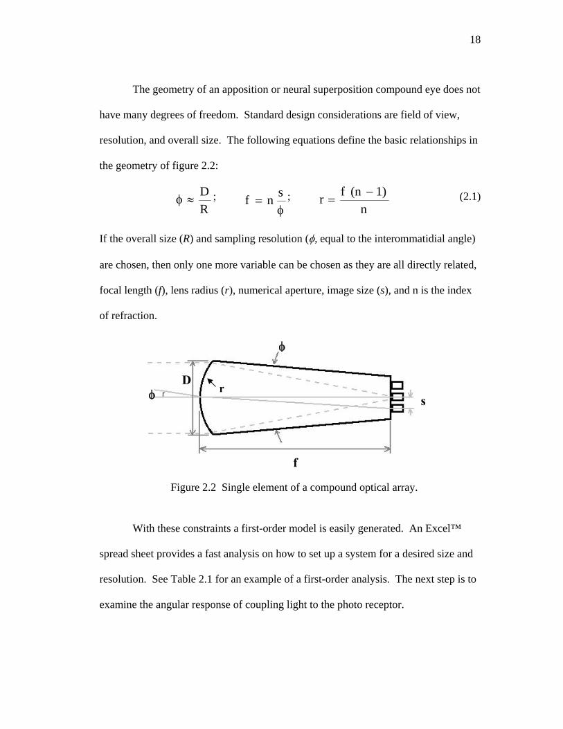
The geometry of an apposition or neural superposition compound eye does not

have many degrees of freedom. Standard design considerations are field of view,

resolution, and overall size. The following equations define the basic relationships in

the geometry of figure 2.2:

RD

≈φ ; φ

=snf ;

n1)(nfr −

= (2.1)

If the overall size (R) and sampling resolution (φ, equal to the interommatidial angle)

are chosen, then only one more variable can be chosen as they are all directly related,

focal length (f), lens radius (r), numerical aperture, image size (s), and n is the index

of refraction.

φ

D

With these constraints a first-order model is easily generated. An Excel™

spread sheet provides a fast analysis on how to set up a system for a desired size and

resolution. See Table 2.1 for an example of a first-order analysis. The next step is to

examine the angular response of coupling light to the photo receptor.

f

φ s

Figure 2.2 Single element of a compound optical array.

r

19

Table 2.1 First-order layout for a compound optical array.

20

D ∆pwave Airy Disk

λ /d

∆pray f

d/f

d

∆ p2 ~ ∆pwave2 + ∆pray

2

Figure 2.3 The acceptance angle (∆p)of an ommatidium results from a combination of the Airy diffraction pattern (point-spread function) given by λ/D and the geometrical angular width of the rhabdom d/f as the nodal point of the lens.

There is an abundance of research on the angular responses of apposition

compound eyes and a few comparisons with laboratory simulations [2.1-2.4]. Natural

systems are near diffraction limited and are similar in response to coupling light into

single mode fiber, see figure 2.3. They typically have Gaussian angular responses

[2.4], with varying amounts of crossover between ommatidia [2.5]. The assumption

tends to be that the interommatidial angle is closely matched to the 50% overlap of

the neighboring ommatidal angular responses. The resolving power of the compound

eye depends on the relationship between the interommatidial angle and the angular

sensitivity of the rhabdom. The highest resolvable frequency as defined by the

21

Nyquist criterion is, )2(1

φ=sv , assuming that that the angular sensitivity response

is narrow relative to the interommatidial angle. Taking motion into consideration it is

important to note that motion of just 1/10 the resolvable frequency can be detected.

This phenomenon is explained by hyperacuity [2.4,2.6], but does not improve the

ability to resolve complex scenes, patterns, or objects.

The angular response in larger artificial systems is much more flexible. In the

smallest of natural compound eyes, the fact that the nearly diffraction limited spot is

close to the same size as the rhabdomere leads to the angular acceptance response

always having a Gaussian profile. Even slightly larger size means that there is much

more room to tailor a unique angular acceptance response. For example, the blur spot

can be much smaller than the detecting media, or fiber optic, creating a flat top

response with sharp cutoffs.

2.2 Apposition and Neural Superposition model simulations

The Excel table was expanded to generate a more complete geometrical

model for either apposition or neural superposition systems (Table 2.2). Data from

the table are then transferred to LightTools®, an optical modeling software package

from Optical Research Associates, to generate a detailed optical analysis and make

any modifications for performance requirements.

22

Physical Properties Design Specifications

System Radius (mm)* 60 Resolution Inter ommatidial angle (deg)* 3Lens Index* 1.41 (overlap) 3.46 Central Field (deg) 3.00Lens Diameter (mm)* 2.5 Off-axis field (deg) 3.00Lens Spacing (mm) 3.14 Hyperacuity Lens curvature (radius mm)* 2.06 Off-axis Field shift (deg) 0.13Lens height (mm) 0.42 Marginal focus (mm) 6.38Distance to image plane (mm)* 6.45 Full Fill B (bestfocus mm) 6.96 Paraxial focus (mm) 7.1Central fiber core dia. (mm)* 0.24 Cent. fiber clad dia* 0.25 Off-Axis fiber core dia* 0.24 Off-Axis fiber clad dia* 0.25 Fiber NA (deg)* 30.66 NA in lens (deg) 21.2

* Indicates a user entered value

Table 2.2 Revised layout for a compound optical array, neural superposition included.

23

Various modifications of the geometrical model can be used to tailor a desired

response performance. The response may need to match a natural system or be

customized for a unique optical or signal processing solution. By changing physical

properties of focal length, lens curvature, detector size and position, an artificial

system is easily customizable. Additional methods of customization include;

specifying aberrations in the optic(s), using a gradient index media, or adding

secondary optics. Figure 2.4 shows Gaussian, top hat, and triangular angular

acceptance functions generated by varying a compound optical array model in this

thesis. As the width of the angular acceptance function is manipulated the

interommatidial angle must be changed also. If the angular acceptance increases

above the interommatidial angle the highest resolvable frequency is reduced.

Figure 2.4 Customized angular acceptance functions.

24

Figure 2.5 is a LightTools model based on the work of Steven Barrett’s group

at the University of Wyoming. It is designed to produce an angular response similar

to the house fly Musca domestic [2.4]. Figure 2.6 shows the Gaussian response of

neighboring photoreceptors with ~75% overlap as a source is scanned across the

field. This is an excellent example of how an artificial compound optical array can be

modeled to provide a specific layout, resolution, and tailored angular response. In

this case, one that matches the near diffraction limited optics of a natural system. It is

also clear that there is a significant loss of photons with this method.

Figure 2.5 University of Wyoming artificial neural superposition optical design. Left, 12mm diameter plano-convex lens. Right, three

1mm optical fibers with spherical ball lenses.

25

Illuminance vs Field

0.0E+00

5.0E-05

1.0E-04

1.5E-04

2.0E-04

2.5E-04

3.0E-04

-8 -6 -4 -2 0 2 4 6 8

Field Position (deg)

Illum

inan

ce T

otal

Pow

er

Figure 2.6 Angular acceptance function of optical system in Figure 2.5

The rest of this section shows an example of how the system responds to

changes in its physical geometry. This helps to explain how to customize the system

for a desired signal response as well as providing a set of tolerances for design

sensitivity. Figure 2.7 shows a seven ommatidia mockup generated in LightTools®

to carry out the following simulations. In the first case, the lens radius (r) of the

system is varied to study the effects of defocusing the light on photoreceptors of a

fixed position. In this model the photoreceptors are simulated as fiber optics with a

receiver at the end. Figure 2.8 shows the photoreceptor response to scanning a 1mm

26

circular lambertian source across the visual field, at both 20cm from the system and at

infinity for different values of r.

Figure 2.7 Neural Superposition Model LightTools® The right image shows the fiber bundles in the three vertical ommatidia. The three numbered fibers collect light

from the same field.

In the second case, the lens radius is held constant, and the position (f) of the

photoreceptor bundle is varied to study the effect on the photoreceptor’s angular

response. Figure 2.9 shows the behavior of the system to a 1mm circular source

scanned across the visual field at both 20cm from the system and at infinity for

several different values of f. Take note that in the case of an apposition system

changing the position of the photoreceptors will result only in changing the overlap of

neighboring responses and their photoreceptor response profile, but in a neural

superposition system it will also slightly misalign photoreceptors that shared the same

field of view. This is clearly visible in figure 2.9 as the peak of the two outer angular

response curves shift with the changes in position. However, research suggests that

such misalignment can be beneficial for the detection of motion [2.5].

27

Radius Defocus Studysource @ 20cm

0.0E+00

5.0E-06

1.0E-05

1.5E-05

2.0E-05

2.5E-05

3.0E-05

-6 -4 -2 0 2 4 6

Angle(deg)

Illum

inan

ce(W

)

R=1.96mmR=2.06mmR=2.16mmR=2.26mmR=2.36mmR=2.46mm

Radius Defocus StudySource @ Infinity

0

0.05

0.1

0.15

0.2

0.25

-6 -4 -2 0 2 4 6

Angle(deg)

Illum

inan

ce(W

)

R=1.96mmR=2.06mmR=2.16mmR=2.26mmR=2.36mmR=2.46mm

Figure 2.8 The response of receivers 1, 2, and 3 in the same ommatidium as radius of curvature changes from 1.96-2.46mm.

Angle denotes the field position of the source where zero degrees is centered over receiver 2.

28

Focal Length Defocus StudySource @ 20cm

0.0E+00

5.0E-06

1.0E-05

1.5E-05

2.0E-05

2.5E-05

3.0E-05

-6 -4 -2 0 2 4 6

Angle (deg)

Illum

inan

ce (W

)

5.96.16.36.56.77.1

Focal Length Defocus StudySource @ Infinity

0

0.05

0.1

0.15

0.2

0.25

-6 -4 -2 0 2 4 6Angle (deg)

Illum

inan

ce (W

)

5.96.16.36.56.77.1

Figure 2.9 The response of receivers 1, 2, and 3 in the same ommatidium as focal length changes from 5.9-7.1mm. Angle denotes the field position of the source where zero degrees is

centered over receiver 2.

29

The response curve is the convolution of the irradiance distribution at the

receiver plane with the pupil function of the receiver. The receiver in this case is a

circle function. Changing the radius of curvature or position of the detectors

manipulates the irradiance distribution at the entrance of the fiber.

The radius of curvature study shows that the shape of the angular response,

and the amount of overlap can be manipulated. There are flat top, triangular and

Gaussian like shapes. There is a significant amount of defocus necessary for a

Gaussian or triangular shape which results in loosing half or more of the light

throughput. In an apposition system this light is lost, but in a neural superposition

system a portion is captured by the surrounding rhabdom. The shape of the angular

response curve is generally more Gaussian in all of the 20cm object distance

measurements. The receiver position study shows similar results. Profiles in the

20cm test remain mostly Gaussian like, but when the source is at infinity several

profiles are possible.

2.3 Design limitations of compound optical arrays

It is important to discuss the limitations of compound optical arrays in order to

find the solution space where a compound optical array is the appropriate solution.

Here the focus is on theoretical limits, while manufacturing issues are discussed in

later chapters.

30

Many natural compound eyes are near the diffraction limit for the visible

spectrum. The corneal lens diameter is 20-50 microns, focal lengths 45-250 microns,

and the rhabdom are typically in the range of one to two microns in diameter. For

artificial designs, miniaturization begins with the spectral range, effecting material

and detector choices that will in turn set the diffraction limited spot size.

For artificial compound designs that are not diffraction limited, like the one

discussed in the previous section, the most profound limitation to compound eyes is

spatial resolution. An average insect has a spatial resolution around 1 cycle per

degree, very poor compared to a human’s 60 cycles per degree [2.11]. In order to

improve the resolution the size of the eye must increase, but this is where compound

eyes eventually become impractical.

The radius of a compound eye is:

sDvR 2≈ or, φ/DR ≈ , ⎟⎠⎞⎜

⎝⎛ = )2(

1φsv (2.2)

where R is the radius, φ is the inter-ommatidial angle, D is the pupil lens diameter of

each ommatidia, and vs the sampling frequency (see figure 2.1). For a diffraction

limited system the acceptance angle is roughly Δρ ≈ λ/D, and the acceptance angle

matches the inter-ommatidial angle (φ = Δρ). Then D can be substituted into equation

one, yielding the relation:

(2.3) 24 svR λ≈

For camera eyes, like our own human eye, the relationship between eye radius and

sampling frequency is:

31

( ) svfR λ/#≈ (2.4)

The size of a simple eye increases linearly with resolution, whereas the compound

eye increases as the square of the spatial resolution. This is the common explanation

as to why all large eyes are camera type eyes, and is covered in greater detail in

several references [2.7-2.9].

The compound eye still has its advantages. It has an almost uninterrupted full

field of view. It saves space and weight because it does not require an enclosure, or

extended imaging distance. Aberrations can become a problem in large eyes, but are

negligible in compound eyes because of their short focal length. Also, compound

eyes have a great depth of field extending from a few millimeters to infinity. This

leads to an interesting point made by Wehner [2.10], “a bee scanning objects parallel

to the horizon exhibits an angular resolution 160 times poorer than man. A bee can

resolve the same number of points as we do by just viewing the object from a distance

160 times smaller.”

32

2.4 Concluding remarks

Artificial compound optical arrays can be manipulated further to create much

more complicated designs. In this thesis, only matching ommatidial elements are

used in spherical or circular layouts so as not to violate any basic principles or

inherent assumptions of the basic compound eye functionality. Custom designs can

continue to explore the effects and uses of designing variations in ommatidial angle,

manipulating the radius of eye, varying the angular acceptance between ommatidia,

and perhaps using photoreceptor layouts not found in nature. In chapter 4 this thesis

will explore tapered gradient index lenses, another variable that can be used in the

design of compound arrays. Incorporating a gradient index into an artificial system

provides an additional degree of freedom that can be used to fine tune focal length,

image size, and numerical aperture. For an artificial system it may be advantageous

to use a gradient index to shorten the focal length to reduce volume, or increase the

numerical aperture.

2.5 References

2.1 G. A. Horridge , “The Separation of Visual Axes in Apposition Compound

Eyes”, Philosophical Transactions of the Royal Society of London. Series B,

Biological Sciences, Vol. 285, No. 1003 (Dec. 5, 1978), pp. 1-59

2.2 Adrian Horridge, “The spatial resolutions of the apposition compound eye and

its neuro-sensory feature detectors: observation versus theory”, Journal of

Insect Physiology, Volume 51, Issue 3, March 2005, Pages 243-266

33

2.3 A Brückner, J Duparré, A Bräuer, A Tünnermann , “Analytic modeling of the

angular sensitivity function and modulation transfer function of ultrathin

multichannel imaging systems”, OPTICS LETTERS, Vol. 32, No. 12, June

15, 2007

2.4 D T Riley, W M Harman, E Tomberlin, S F Barrett, M Wilcox, C H G

Wright, “Musca Domestica Inspired Machine Vision with Hyperacuity”, SPIE

proceedings Smart sensor technology and measurement systems. Conference,

San Diego CA, 2005, vol. 5758, pp. 304-320

2.5 B Pick, “Specific Misalignments of Rhabdomere Visual Axes in the Nerural

Superposition Eye of Dipteran Flies”, Bilogical Cybernetics, 26, pg 215-224,

1977

2.6 T. Poggio, M. Fahle, and S. Edelman, “Fast perceptual learning in visual

hyperacuity” Science, Vol 256, Issue 5059, 1018-1021, © 1992 American

Association for the Advancement of Science

2.7 K. Kirschfeld, “The Resolution of Lens and Compound Eyes”, Neural

Principles in Vision (Eds. F. Zettler, R. Weiler), pg 354-370, 1976

2.8 M Land, Facets of Vision (Eds. D.G. Stavenga, R.C. Hardie), “Variation in

the structure and design of compound eyes”, Chap 5, pp 90-111, 1989

2.9 Kazunori Hoshino, Fabrizio Mura, Isao Shimoyama, “Design and

Performance of a Micro-Sized Biomorphic Compound Eye with a Scanning

Retina”, Journal of Microelectromechanical Systems, Vol.9(1), 2000 IEEE

2.10 R. Wehner, “Comparative Physiology and Evolution of vision in

Invertebrates”, Vol. VI/C, Invertebrate Visual Centers and Behavior II,

Spatioal Vision in Arthropods, Springer-Verlag, New York, 1981

2.11 M F Land, D E Nillson, Animal Eyes, Oxford University Press, 2002

34

Chapter 3

Artificial Apposition System

3.1 Concept

A proof of concept apposition compound optical array is built to demonstrate

the design and modeling steps from chapter 2. The motivation is to investigate a low

resolution and potentially inexpensive alternative for an application that would

otherwise use a camera style optical system. The potential applications are limited by

the compound eye’s low resolution and small apertures that limit light collection.

The application focused on in this thesis is an optical tracking system with a

designated target. This type of system can be found in unmanned air vehicles

(UAVs), machine vision, and missile guidance systems, but could also be applied to

other guidance and object avoidance technology.

The primary function of the system is to locate and track towards a moving

target. This may require a significant field of view, and mechanical tracking of the

optics is not desirable for keeping the system cheap and light. Weight and size are

the primary concerns as the optical system is to fit to a pre defined volume of space

and has a strict weight budget. High resolution optics are not required and no object

recognition is necessary as the target is designated with a marker to single it out from

35

the rest of the environment. Low resolution, light weight, minimal volume, and a

wide field of view are a combination of requirements within the compound optical

array solution space.

3.2 Apposition and Neural Superposition Designs

The system radius is set at 60mm and the interommatidial at 5 degrees. The

field of view for a 19 element hexagonal array will be 25 degrees. A much larger

field of view is possible with more elements, but not necessary for fabricating a

demonstration prototype. A compound optical array can image to a detector array,

individual receivers, or couple the signal into fiber optics. The use of curved detector

arrays is not yet a viable option, and using imaging optics to relay the output of the

compound array is impractical if the goal is to replace a camera like system.

Commercially available plastic fiber optics are used in this system. This provides a

flexible option open for using individual detectors or coupling the fibers directly to an

array of receivers.

Custom molded optics are used for the array. They are made in a planar mold

and then fit into a housing that can hold the optics and fibers in the correct alignment.

Since the mold is flat, and the housing is spherical, an elastic interconnecting layer is

necessary. Optical quality elastomers are commercially available and used for both

the optics and interconnecting layer.

36

Provided these constraints and materials the other design specifications can be

calculated for an apposition or neural superposition design using the methods

described in chapter 2, and the system modeled in LightTools®.

Figure 3.1 is the nineteen element apposition prototype designed in

LightTools®. The specifications are given in Table 3.2.1.

Figure 3.1 Nineteen element apposition compound optical array designed in LightTools®.

37

Table 3.2.1 Apposition array specifications

Physical Properties Design Specs System Radius (mm) 60 Resolution

Inter ommatidial angle (deg) 5

Lens Index 1.41 (overlap) 5.77 Central Field (deg) 7.93Lens Diameter (mm) 3.5 Off-axis field (deg) 0Lens Spacing (mm) 5.23 Hyperacuity Lens curvature (radius mm) 2.6

Off-axis Field shift (deg) -0.95

Lens height (mm) 0.67 Marginal focus (mm) 7.8Distance to image plane (mm) 10

Full Fill B (bestfocus mm) 9.8

Paraxial focus (mm) 8.94Central fiber core dia. (mm) 0.98 Cent. fiber clad dia 1 Off-Axis fiber core dia NA Off-Axis fiber clad dia NA Fiber NA (deg) 30.66 NA in lens (deg) 21.2

38

Figure 3.2 is a nineteen element LightTools neural superposition model.

Each ommatidia supports seven fibers, requiring a total of 133. Specifications of the

ommatidia and fibers are provided in Table 3.2.1. It has equal resolution to the

artificial apposition system, and the overall field for a nineteen element system is 25

degrees plus another +/-5 degrees of under sampled region from the off axis fibers in

the outer ring of ommatidia. The specification in Table 3.2.1 uses seven 250um

diameter fibers located at a shorter focal length. The shorter focal length also results

in a corneal lens with stronger curvature. A larger fiber bundle solutions exists, but

the width of the fiber bundles can not exceed the physical width of the ommatidium.

For example, 1mm diameter fibers do not fit because the diameter of the fiber bundle

exceeds the diameter of the ommatidia at the focal position.

39

Figure 3.2 Nineteen element neural superposition compound optical array designed in LightTools®

40

Table 3.2.2 Neural Superposition Array Specifications

Physical Properties Design Specs System Radius (mm) 60 Resolution

Inter ommatidial angle (deg) 5

Lens Index 1.41 (overlap) 5.77 Central Field (deg) 4.95Lens Diameter (mm) 2 Off-axis field (deg) 4.95Lens Spacing (mm) 5.23 Hyperacuity Lens curvature (radius mm) 1.3

Off-axis Field shift (deg) 0.062

Lens height (mm) 0.47 Marginal focus (mm) 3.69Distance to image plane (mm) 4

Full Fill B (bestfocus mm) 4.09

Paraxial focus (mm) 4.47Central fiber core dia. (mm) 0.245 Cent. fiber clad dia 0.25 Off-Axis fiber core dia 0.245 Off-Axis fiber clad dia 0.25 Fiber NA (deg) 30.66 NA in lens (deg) 21.2

41

Due to the number of fibers in the neural superposition design and potential

issues with aligning and managing them, only a prototype apposition compound array

is fabricated.

The designed system is relatively large compared to natural compound eyes.

Typically, compound optical arrays have the most advantage over traditional camera

systems when their size is in the range of natural systems. However, compound

optical arrays are completely scalable until they reach the diffraction limit of their

operational spectral range. Even though this system is large, and at its current size is

likely outperformed by alternate optical systems, the entire design can be scaled down

to a much smaller size and still have the same performance. So the design is still

considered valid, and is just fabricated and tested at a much larger scale.

Manufacturing a system like this on a scale even near an insect eye has never been

done and is outside the scope of this thesis. The size chosen for the prototype is very

convenient for manufacturing. The tolerances are manageable and the components

are standard commercially available products. Special manufacturing methods and

equipment are not required for the fabrication and assembly process.

42

3.3 Construction

The optical material for the lenses is a silicone elastomer (NuSil, R-2615

index of refraction n = 1.41). It is a two part thermal setting elastomer. The fibers

come from Edmund Optics (J02-534). The cladding is 1mm diameter with index

1.402, the core diameter is 980um with index 1.492. The frame and holder are

custom components manufactured by Design Prototyping Technologies (DPT, 6713

Collamer Rd. East Syracuse, NY 13057) using stereolithography (SLA).

The top mold, the lens array side, is made out of the silicone elastomer. To

make the silicone mold, first a positive needs to be made. A pattern mask with the

layout of the corneal lenses is printed onto a transparency (a cellulose acetate sheet

used with overhead projectors) using a laser jet printer. The toner on the transparency

is hydrophobic and traps droplets of ultraviolet curable resin at the lens positions.

The appropriate volume of UV curable resin (Norland 61) is dispensed onto the

transparency in the positions of the corneal lenses.

)3(

61V 2 hRh −= π ; (3.3.1)

V is the volume of UV curable resin, h is the height of the lens, and R is the radius of

curvature of the lens.

After curing the droplets onto the transparency, the silicone elastomer is

poured over the mask. The silicone cures at room temperature in 24 hours, or in 15

43

minutes at 100oC. Once the silicone is fully cured, the transparency is peeled off,

leaving the silicone negative mold for the lens portion of the array.

The bottom mold, for the inner side of the array, and the housing for the

finished array are made out of polyurethane by Design Prototyping Technologies’

stereo-lithography process. This bottom mold and the housing have 1mm through

holes centered at the back of each cone where the fibers are inserted.

The two molds are spaced apart by plastic shim stock (250μm) and held in

position by an aluminum frame. A piece of glass is placed between the aluminum

frame and the silicone to keep the silicone from flexing. The mold is filled with the

optical silicone elastomer, and centrifugal force is used to remove any air bubbles.

Fibers sections are inserted into the 1mm holes in the back bottom mold. These are

not the final fibers, they are measured and cut sections that will form 1mm holes for

the positions where the final fibers will later be permanently fixed. The fibers are held

in place with a very small drop of superglue. Figures 3.3 and 3.4 show the pieces of

the mold, the frame, and the pattern mask.

Figure 3.3 Casing that holds the mold together while the silicone sets. The yellow block on the left is the back portion of the mold.

44

Figure 3.4 Top left, practice silicone lens array using the front mold and a flat glass back mold. Top right, final negative mold used for the front of the compound optical array. Bottom left, mask with microlenses used for making the mold at top right. Bottom right, a second mask with the 250 micron shim stock

Once the silicone compound array is thermally set, first the fiber pieces are

removed, and then the mold is opened and the array carefully removed. A thin layer

of silicone is applied to the spherical surface of the housing and inside the cones. It is

left to sit for an hour to let any air escape. Then the silicone lens array is carefully

placed into the housing. Any air and extra silicone is gently squeezed out. The top of

the housing is screwed down holding the array tight onto the spherical housing. Then

the fibers are gently inserted through the back of the housing and slid into silicone

45

cones. The fibers should be marked to the approximate depth so that they are not

pushed in too far. This can push the cone out of the holder, and also allow air to get

back in between the cone and the holder. Once a fiber is in place a generous amount

of extra silicone applied that will help hold it in place once set. The unit is left for 24

hours to allow the array and fibers to cure to the housing.

3.4 Results

Figure 3.5 shows a final complete 19 element system, and a seven element

system. During the removal from the back mold the connecting elastomer layer tore

and the ommatidia were taken out individually. Figure 3.6 shows the system with the

fiber bundle.

Figure 3.5 Left, Seven individual silicone ommatidia in a housing. Right, A complete nineteen element silicone apposition compound arrays in the polymer housing. Bottom center, a single silicone ommatidium with a small section of fiber.

46

Figure 3.6 The seven element array with 1mm diameter fibers. The box in the lower right shows the fiber output. Seven fibers from the ommatidia are bright, and the

other fibers that are capped off are dark.

To test the angular response of the system, a HeNe laser was expanded to a 1

inch beam and recollimated. The compound array was placed in the beam on a

rotation stage. As the array is rotated through the beam, the power output of three

fibers belonging to adjacent ommatidia is recorded at half degree intervals.

The angular response curves and overlap match fairly well for the rather crude

fabrication method, see figure 3.7. Molds from Design Prototyping Technologies

have a +/-0.1mm error specification. Some of the holes did not fit the 1mm fibers,

and a 0.98mm drill bit was used to slightly widen them. The cones and the housing

they fit in were 12mm long. A 0.1mm error from the bottom to the top of a cone

47

would result in the interommatidial angle being off by almost half a degree. If the

cone angle and fiber position were both off in the same direction, .2 mm, this would

result in a 1.2 degree error in interommatidial angle. The curves are well within these

error bounds. The fiber mounting was measured out with a micrometer to +/-0.1mm,

and the placement done by hand. Being off by a several hundred microns will not

have a noticeable effect at the 10mm long focal length.

Angular R es pons e of Artific ial Appos ition  Array

0

0.1

0.2

0.3

0.4

0.5

0.6

0.7

0.8

0.9

‐15 ‐10 ‐5 0 5 10

F ie ld  (deg rees)

Power(μW)

15

LE F T 

C E NTE R

R IGHT

L ightTools  Model

Figure 3.7 The Angular response measured across 3 neighboring ommatidia and compared with the LightTools® modeled data.

The left curve in the diagram has a dip at the peak. The dip is about ~8% lower that

the peak. This might indicate a small air gap between the fiber and the silicone, or

perhaps a small air bubble as it was not always possible to get all the air bubbles out

48

of the silicone. Smaller bubbles were often difficult to get off of the inner walls of the

bottom mold. The final curvature and sphericity of the lenses was not measured, but

curvature error or non symmetrical asphericity could account for some of the

asymmetry in the response curves. But there is no drastic change in shape or power,

which suggests that the radius of curvature does not deviate by more that 200μm.

This can be compared with the curvature and position studies in chapter 2.

3.5 Concluding Remarks

A compound eye scenario was presented and apposition and neural

superposition solution designs derived using the methods covered in chapter 2. The

optics of the apposition design were manufactured in a silicone elastomer and housed

in a sterolithography polymer to hold the system in the proper alignment. The

angular response was measured by rotating the system through a collimated HeNe

beam and recording the fiber outputs of adjacent ommatidium.

It would be interesting to return to this work and build a neural superposition

prototype, as well as have the systems paired with a vision processing system. The

paper “Musca domestica Inspired Machine Vision with Hyperacuity” [3.1]

demonstrates the a 2-D neural superposition architecture that can detect motion even

in low light, and low contrast conditions.

49

3.6 References

3.1 D T Riley, W M Harman, E Tomberlin, S F Barrett, M Wilcox, C H G

Wright, “Musca Domestica Inspired Machine Vision with Hyperacuity”, SPIE

proceedings Smart sensor technology and measurement systems. Conference,

San Diego CA, 2005, vol. 5758, pp. 304-320

50

Chapter 4

Tapered Gradient Index Lenses

4.1 Introduction to tapered GRINs

Three common gradient index lens types are radial, axial, and spherical. The

names refer to the shape of the isoindicial surfaces, surfaces of constant index of

refraction. The variation of refractive index normal to the isoindicial surfaces,

referred to as the gradient index profile, is represented with a mathematical function.

For example

Radial: N(r) = N00 + N10 r2 + N20 r4 + …

Axial: N(z) = N00 + N01 z + N02 z2 + …

(4.1)

(4.2)

where N is the refractive index, z is the optical axis direction, r is the distance

perpendicular to the optical axis.

51

These gradient index lens types are a well understood in literature and are all

commercially available. Spherical gradient index lenses exist naturally, like the

octopus eye (Figure 4.1.1).

Figure 4.1.1 The octopus eye and isoindicial surfaces of its spherical gradient index crystalline lens.

The primary element is a spherical gradient index crystalline lens. Other gradient

index profiles in nature typically require a more specific mathematical representation

that combines aspects of radial, axial, and spherical representations. The index

profile of the human gradient index crystalline lens is a more complicated example

(Figure 4.1.2) which is only compounded by the fact that the lens changes shape for

accommodation.

52

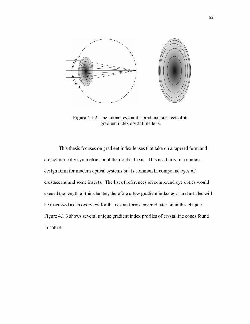
Figure 4.1.2 The human eye and isoindicial surfaces of its

gradient index crystalline lens.

This thesis focuses on gradient index lenses that take on a tapered form and

are cylindrically symmetric about their optical axis. This is a fairly uncommon

design form for modern optical systems but is common in compound eyes of

crustaceans and some insects. The list of references on compound eye optics would

exceed the length of this chapter, therefore a few gradient index eyes and articles will

be discussed as an overview for the design forms covered later on in this chapter.

Figure 4.1.3 shows several unique gradient index profiles of crystalline cones found

in nature.

53

Figure 4.1.3 Left two images: Water-Flea Polyphemus[4.1]. Right two images: Limulus (Xiphosura) [4.2].

Gradients found in apposition eyes, mostly underwater crustaceans, have

many variations. In fact, the compound eye of the water flea Polyphemus has four

different sections, each having a crystalline cone with a different gradient index

profile [4.1]. In general the crystalline cones have a short conical shape. Figure

4.1.3 shows two examples of a fairly common gradient index profiles for apposition

crystalline cones.

54

Superposition crystalline cones, whether insect or crustacean, tend to all have

a similar form shown in figure 4.1.4. They are similar to a short, slightly tapered

radial gradient with some axial components at the ends. An article by P. McIntyre

and S. Caveney [4.4] studies the superposition optics of several beetles. The change

in index of these lenses can exceed 0.15. This is an impressively large number rarely

seen in gradient systems, and even with current technology would be difficult to

replicate in glass or polymers.

Figure 4.1.4 Euphausia superba (Antarctic krill) [4.3]

There are a handful of animals like the butterfly that have long crystalline

cones. These longer cones nearly always exhibit changing gradient index profiles

within a single ommatidium that often morph from one type to another. For example,

a spherical or conically tapered GRIN followed by a radial or axial gradient. Several

examples are show in figure 4.1.5. The butterfly Heteronympha merope is an

apposition eye but its corneal lens and crystalline cone combination is an afocal

55

system (see figure 4.1.6). Derek Bertilone , J.H. Van Hateren and D. E. Nilsson have

shown how this system improves coupling efficiency [4.5, 4.6].

Figure 4.1.5 Gradient index ommatidia. Darker shading depicts higher index of refraction.

Figure 4.1.6 Afocal crystalline cone of the butterfly [4.8]

56

Though tapered GRIN design forms that are found in nature are not common

in modern optical design, there is one form that is quite common and well

documented. This is the tapered radial gradient index rod, and it is the profile formed

when a gradient index fiber is drawn out or molded into a tapered shape. Research on

tapered gradient index fibers dates back to 1970 [4.9], with a complete geometrical

solution of a linear case by J.S.J. Brown in 1980 [4.10], and a parabolic tapered radial

case that has an exact ray path solution [4.11], worked out by D. Bertilone.

z

r

0 2 4 6 8 10 12 14 16 18 20-3

-2

-1

0

1

2

3

No

1.545

1.55

1.555

1.56

1.565

Constant Index of Refraction

No-dn

No-dn

No

Figure 4.1.7 Isoindicial surfaces of a linearly tapered radial gradient index rod.

;

)(),( 2

2

10 zzrNNzrN

o −−= (4.3)

Figure 4.1.7 shows the isoindicial surfaces of a linearly tapered GRIN profile

along the optical axis. N is the index of refraction as a function of r, radius, and z,

distance along the optical axis, where zo is the apex of the tapered cone, No is the base

57

index, N1 is a constant, and dn is the maximum change in index of refraction. This

profile described by equation 4.3 is essentially a radial gradient index lens with a

decreasing radius along the optical axis. It maintains the full index change and

parabolic profile along its length. Tapering a radial gradient causes the period to

shorten and the numerical aperture increases, see fig 4.1.8.

Figure 4.1.8 Shortening periods in linearly tapered radial GRIN rod.

From the paraxial solution derived by S.J.S Brown [4.10] (equation 4.4), the

quarter pitch for a tapered radial is derived as a function of taper angle (equation 4.5).

412);1(~

]];~[*[~2]]~[*[~)(

200

000

0

−Δ

=−=

⎟⎟⎟

⎠

⎞

⎜⎜⎜

⎝

⎛ +−=

aNnbh

zaz

zLogbSinzab

arhuzLogbCoszyzY

(4.4)

⎟⎟⎠

⎞⎜⎜⎝

⎛−

−=

−

1)(]2tan[

0 bbArc

ea

hazπ

(4.5)

Y(z) is the distance from the optical axis to the ray, yo is the starting height of the ray,

uo is the starting angle of the ray, ho is the outer radius of the cone at z = 0, a is the

half angle of the taper in radians, No is the index of refraction along the optical axis,

58

and Δn is the change in refractive index from the center to edge of the cone. The

derivation for the paraxial ray solution of a tapered radial GRIN rod and the quarter

pitch are provided in Appendix A.

The current state of tapered gradient index research falls into two categories,

modeling of tapered gradient index optics as found in animal eyes, and the tapered

radial gradient index. In this case, the tapered gradient device is fabricated by heating

a radial gradient and drawing it into a cone. This device was used in the telecom

industry. Animal eye gradient index modeling is a relatively small are of activity,

even for the human crystalline lens, which has only recently made large

advancements toward a comprehensive model [4.12, 4.13].

There is a large gap between the two areas. The tapered radial model is well

documented and manufacturable but its profile does not fully encompass

measurements of tapered gradients in nature. The difference is inherent in the way

tapered radial gradients are manufactured versus the way animal gradient index cones

are grown. A tapered radial starts out as a cylindrical rod or fiber with a radial GRIN

profile. It is then extruded or molded into a tapered shape with a thermal process.

This essentially maintains the radial profile and index change while the outer

cylindrical profile takes on a tapered form. In an animal eye, the gradient index is

created by varying protein concentrations in cellular membranes. As the cells grow,

or new cells form, the gradient index forms layer by layer, often compared to onion

layers in the case of the human crystalline lens. These layers tend to have nearly

continuous bounds and are analogous to isoindicial surfaces. Because of the way the

59

gradient index grows in animals, they have significant axial and radial variations.

The complexity and diversity of tapered gradients in nature has resulted in them being

examined on a case by case basis, as well as making them less attractive for

manufacturing.

The remaining chapters focus on two areas that have not been previously

explored, a study of cylindrically symmetric tapered gradients that have radial and

axial dependence, and the fabrication of similar gradients. This chapter explores

tapered gradients that have both radial and axial components and compares them with

radial and tapered radial gradients. Also, further in, a general form for representing

and modeling gradient elements with more complex profiles like those found in some

animals is developed. Chapter 5 will cover the fabrication of tapered gradients in

polymers via liquid monomer diffusion.

4.2 A study of tapered gradient index profiles

The goal of this study is too examine the behavior of light as it propagates in

tapered gradient index profiles with both radial and axial components. Two

cylindrically symmetric tapered gradient index profiles are described and compared to

a radial gradient and a linearly tapered radial gradient, as these are two standards that

are well documented in theory and practice. This is the first study of its kind to

60

examine the specific optical effects induced with combined axial and tapered radial

gradient index components.

Several factors are used to constrain the study. The tapered profiles are

bounded by a linear slope, a cone shape, the same as the linearly tapered radial

gradient. The axial gradient profile is constrained by the maximum change in

refractive index. The radial gradient profile is equal in all four cases, represented by

equation 4.1, and bounded by the maximum change in index, but when higher order

terms are used, the coefficients are allowed to vary between designs. There are many

possible gradient index profiles that fit these bounded conditions but the two used

here are basic forms, one with a linear axial component the other quadratic axial

component. There are two main reasons for these selections. First, the basic forms

make it easier to attribute optical effects to the mathematical representation of the

gradient index profile. Second, these particular forms are useful in representing the

gradient index profile achieved by monomer diffusion into a tapered polymer cone.

The new tapered gradients will be referred to as the hyperbolic tapered radial

gradient (H-TR GRIN), and the sloped tapered radial gradient (S-TR GRIN). The H-

TR GRIN has a quadratic axial component, and due to the constraints imposed above

the function defining the gradient index profile becomes a hyperbolic function, see

figure 4.2.1c. The S-TR GRIN has a linearly decreasing axial component, a constant

‘slope’ down the optical axis, see figure 4.2.1d. Figure 4.2.1 shows the four gradient

index profiles, H-TR GRIN(c), S-TR GRIN(d), TR-GRIN(tapered radial, b), and the

Radial GRIN(a). Contour lines represent isoindicial surfaces, and the sub plot shows

61

the radial gradient index profiles along the optical axis. Here are the functions that

define each gradient index profile:

Hyperbolic (H-TR GRIN) ⎟⎟

⎠

⎞⎜⎜⎝

⎛+

−−Δ+= 2

2

2

2

0)(1),(

oo

o

hr

zzznNzrN ; (4.2.1)

Sloped (S-TR GRIN) ⎟⎟

⎠

⎞⎜⎜⎝

⎛+

−Δ+=

ooo zz

zzhrznNzrN

)(),( 2

20

0 ; (4.2.2)

Tapered Radial (TR GRIN) ...

)(),( 2

22

0 +−

Δ+=zzh

rznNzrNoo

o (4.2.3)

Radial GRIN ...),( 2

2

0 +Δ+=oh

rnNzrN ; (4.2.4)

Where N is the index of refraction as a function of r, the distance from the optical

axis, and z, optical direction, where zo is the location of the apex of the tapered cone,

No is the index of refraction at r = z = 0, ho is the maximum radius of the cone, and

Δn is the maximum change in index of refraction.

62

(a) Radial GRIN Profile

(b) TR-GRIN Profile

(c) H-TR GRIN

(d) S-TR GRIN Figure 4.2.1 Gradient index profiles.

Left plots: Cross section along the axis, light travels from left to right. Lines represent contours of constant index. Right plots: Radial index profiles along the

axis. The widest profile is from z = 0. The thinnest is from z = 20.

0 2 4 6 8 10 12 14 16 18 20-3

-2

-1

0

1

2

3

-2 0 21.54

1.545

1.55

1.555

1.56

1.565

1.57

0 2 4 6 8 10 12 14 16 18 20-3

-2

-1

0

1

2

3

-2 0 21.54

1.545

1.55

1.555

1.56

1.565

1.57

N

0 2 4 6 8 10 12 14 16 18 20-3

-2

-1

0

1

2

3

-2 0 21.54

1.545

1.55

1.555

1.56

1.565

1.57

0 2 4 6 8 10 12 14 16 18 20-3

-2

-1

0

1

2

3

-2 0 21.54

1.545

1.55

1.555

1.56

1.565

1.57

63

The first data sets examine quarter pitch behavior with a Δn of -0.03 and taper

half angle of ~5.7degrees. In order for the light to image on the back surface of the

tapers under these conditions, the field is +/- 3degrees as limited by the H-TR GRIN.

Table 4.2.1 lists the physical properties of the GRIN models. Set A is a comparison

of lens data and Seidel aberrations when the spherical aberration is eliminated on axis

by changing the 4th order radial profile (they system is weighted for the on axis field).

Set B is the same system where the 4th order term is allowed to vary to achieve the

best focus for all fields (fields are weighted equally). Values generated in Code V®

(Optical Research Associates) assume that an image plane is in air.

Table 4.2.1 CodeV® Specifications

No 1.57 Taper (deg) 5.75

Δn -0.03 ho (mm) 2.5

Ent. Pupil Dia. 2.5 zo (mm) 25

Fields (deg) 0,1.5,3 Wavelength(nm) 632.8

64

Figure 4.2.2 Set A

SET A

-0.005

-0.004

-0.003

-0.002

-0.001

0

0.001

0.002

0.003

0.004

0.005

Sphe

rical

Com

a

T As

tig

S As

tig

Dist

ortio

n

(mm

)Radial GRIN

H-TR GRIN

S-TR GRIN

TR GRIN

0

5

10

15

20

25

F/# EFL(mm) OAL (mm)

Radial GRIN

H-TR GRIN

S-TR GRIN

TR GRIN

00.050.1

0.150.2

0.250.3

0.35

0.40.450.5

Image h(mm)

65

Figure 4.2.3 Set B

Set B

-0.005

-0.004

-0.003

-0.002

-0.001

0

0.001

0.002

0.003

0.004

0.005

Sphe

rical

Com

a

T As

tig

S As

tig

Dist

ortio

n

(mm

)

Radial GRIN

H-TR GRIN

S-TR GRIN

TR GRIN

0

5

10

15

20

25

F/# EFL(mm) OAL (mm)

Radial GRIN

H-TR GRIN

S-TR GRIN

TR GRIN

00.05

0.10.150.2

0.25

0.30.350.4

0.450.5

Image h(mm)

66

The next data set examines the effect of taper angle on the quarter pitch of the

three tapers. For this set the Δn is increased to (-0.06) so effects of faster tapers can

be observed.

Figure 4.2.4 Quarter Pitch vs. Taper Angle

Quarter Pitch vs Taper Angle

8

9

10

11

12

13

14

0 2 4 6 8 10 12 14 16

Angle (degrees)

QP

(mm

)

H-TR GRIN

S-TR GRIN

TR-GRIN

Radial GRIN

For tapers with less than one degree half angle, and with large Δn, the light

experiences multiple periods in the tapers. In figure 4.2.5, the effect of the tapering

for consecutive periods is clearly visible. For the tapered radial GRIN in particular,

the periods shorten relatively quickly, and the increased magnification in turn causes

the numerical aperture to increase.

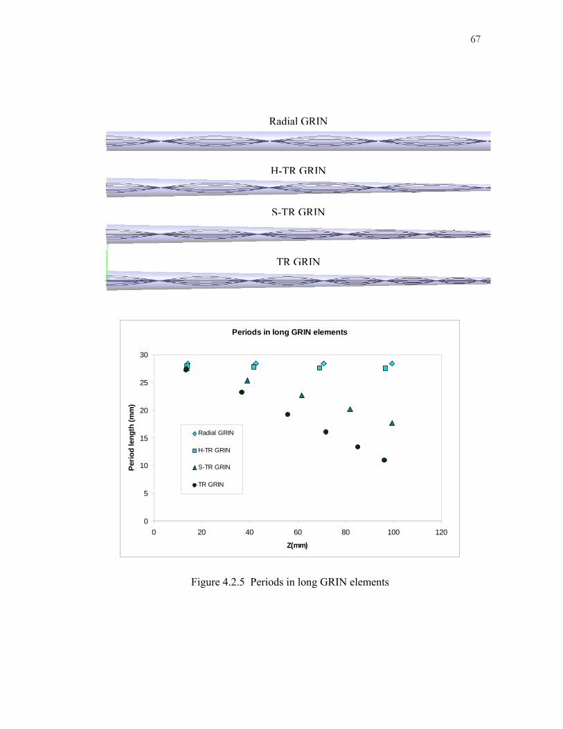
67

Figure 4.2.5 Periods in long GRIN elements

Periods in long GRIN elements

0

5

10

15

20

25

30

0 20 40 60 80 100 120

Z(mm)

Perio

d le

ngth

(mm

)

Radial GRIN

H-TR GRIN

S-TR GRIN

TR GRIN

Radial GRIN

H-TR GRIN

S-TR GRIN

TR GRIN

68

What is immediately apparent in the results is that the radial gradient and

hyperbolic tapered radial gradient are nearly identical in behavior, but the H-TR

GRIN and S-TR GRIN have clear differences. Looking at the isoindicial surfaces in

figure 4.2.1 it is not an obvious conclusion. Going back to the equations for the

profiles gives more insight into this behavior. The TR GRIN and S-TR GRIN both

have radial terms r, that are dependant on the axial term z. The H-TR has a radial

term Δn*r2/ho2 that is the same as a radial gradient index, and an axial term Δn*(zo-

z)2/zo2, but no cross terms. An axial gradient does not provide any power, so based

on the radial component the H-TR GRIN behaves like the radial gradient. A second

look at the radial profiles also helps to explain the phenomenon. Figure 4.2.6 is a

detailed view of figure 4.2.1c subplot. Although consecutive radial profiles along the

axis decrease in index of refraction the shape of the profiles is unchanged. The

bending of light in a gradient index medium is a function of the change in index, the

derivative of the index profile, and since the shape of the radial index profile in both

gradients does not change, the amount of bending is equal.

As the results show, the H-TR GRIN and radial grin are not completely

identical. The axial component does have an effect. In a radial gradient, the period

that light reimages along the optical axis is linearly related to the index. Likewise, in

the H-TR GRIN as the index decreases along the axis, the period also decreases. The

larger the Δn, the more an H-TR GRIN deviates from the radial GRIN.

69

-3 -2 -1 0 1 2 3-0.03

-0.025

-0.02

-0.015

-0.01

-0.005

0

Radius (mm)

Del

ta N

GRIN profiles along the optical axis for aHyperbolic Cone

Figure 4.2.6 Detail of Figure 4.2.1c H-TR GRIN radial profiles. The top curve is the profile at the entrance face. The bottom curve is the profile at the

output face.

4.3 Modeling complex tapered gradient index profiles The hyperbolic and sloped tapered radial GRINs are good starting points for

understanding tapered gradients, and are particularly appropriate for evaluating

experimental results in later chapters; however, they are relatively simple, and for

modeling more complex systems, like a tapered afocal crystalline cone, or diffusion

gradient index optics with changing boundary conditions, a more complete

representation is required. This section discusses potential methods for research that

may continue outside this thesis and would require more complicated models.

70

The solution for most systems is a general form for representing cylindrically

symmetric gradient index profiles as presented in equation 4.3.1. This form allows

for any equation p(z) that bounds the edge (maximum radius), any axial index profile

g(z) along the optical axis, and any constant radial index profile f(r) along the optical

axis. To bound the radial index profile to the edge boundary, it is represented as

f(r/p(z)).

⎟⎟⎠

⎞⎜⎜⎝

⎛⎟⎟⎠

⎞⎜⎜⎝

⎛−Δ+=

)()(1),( 0 zp

rfzgnNzrN ;

00 zz ≤≤ , 1)(0 ≤≤ zg , 1)(

0 ≤⎟⎟⎠

⎞⎜⎜⎝

⎛≤

zprf , and )(0 zp≤ ;

(4.3.1)

It can easily be shown that all the equations in section 4.2 can be represented in this

form. For example, if g(z) is constant, the boundary p(z) is constant, both equal to 1,

and f(r) is quadratic (1-r2), then it reduces to equation 4.2.4, the radial gradient index

profile.

The general layout of the equation can be manipulated, but this particular

form is particularly useful for representing gradient index profiles that are shelled

systems, like crystalline lenses in nature, as well as lenses that are fabricated using

diffusion. The refractive index is properly bounded by the base index No and the

maximum index change Δn. The physical boundary is represented by P(z). The

equations g(z) and f(r) represent the diffusion profile, or in real time diffusion can be

adjusted to incorporate the diffusion coefficient dependence on space or time.

71

Figure 4.3.1 presents a few examples of approximated gradient index

profiles that can be generated with this form and modeled in an optical software

package like Code V® or LightTools®. Using this form is adequate for modeling

most any gradient index eye found in nature, as well as cylindrically symmetric

gradient index optics.

72

Superposition Crystalline Cone (see figure 4.1.4)

Butterfly Afocal Crystalline Cone (see figure 4.1.6)

Clear Apposition Eye Crystalline Cone (see figure 4.1.5 right image)

Figure 4.3.1 Simulated Animal GRIN elements

73

This method still has limitations. It only covers cylindrically symmetric

cases, and assumes the radial profile can be represented by a smooth or piecewise

equation f(r). Systems that lack symmetry or include other variables that are not

easily fit into equation form require a more specific representation. In such cases

there is a rather straight forward method for modeling such systems in Code V® or

LightTools®, although it is computationally intensive and to the extent it is pursued

in this thesis, there remains a significant speed bottleneck when compared to using

the general equation form.

By representing a complex gradient index profile as a matrix or mesh of index

data, the index of refraction information, and partial derivatives along a specific ray

path can be calculated via methods of interpolation. MATLAB® is an excellent

resource for both the representation and interpolation of gradient index profile data in

this form as the tools are already built in. The matrix of data points in 2D or 3D can

be generated in MATLAB® or imported from another program or file. For example,

phase information from interferograms, thermal gradients, or mechanical stress data

from a finite element model can all be imported into MATLAB® and expressed in

the appropriate index data form.

At this point numerical methods can be used to trace rays in MATLAB®;

however, for designing and optimizing an optical system, it is much more beneficial

to model and analyze the ray data in a professional optical software package. Optical

Research Associate’s Code V® and LightTools® packages are both equipped to

access MATLAB® via the COM (component object model).

74

LightTools® uses the Sharma ray trace method [4.14] to quickly calculate ray

paths in gradient index materials. This is a numerical technique that requires the

index profile as a function of x, y, and z, and also the gradient of the index with

respect to x, y, and z. Usually the usergrin.dll (dll stands for dynamically linked

library), provided in the software, is used to represent the gradient in equation form as

well as any necessary coefficients that constrain or define the system. An alternate

option is to use the COM to retrieve the data from another program. With this

method the optical software can utilize MATLAB®’s functions to extrapolate data

and then retrieve the index of refraction information that it requires to trace rays.

Appendix B shows sample code that was written into the LightTools® usergrin.dll.

Figure 4.3.2 is a diagram illustrating the process.

75

Figure 4.3.2 LightTools® gradient index ray trace flow chart. The LightTools® process operates independently in normal operation.

76

This technique is slower since the interpolation methods add significant

computational time, but there is an additional bottleneck inherent in the way the COM

is being used to run an M-file in MATLAB®. Normally it is used occasionally to

import a file or run a program. Instead, it is being used to tell MATLAB® to run the

M-file again and again with each step of the ray, which can increase the time to trace

a ray by a factor of 102 to 103.

The process can be significantly improved with additional work. Code can be

written so the usergrin.dll can read the matrix data and do its own interpolation. An

alternative could be to send the geometry and ray data to MATLAB®, and let it

conduct the interpolation and ray tracing through the GRIN materials, and then return

the resulting ray data.

A valuable addition would also be to include real and imaginary index of

refraction values to incorporate polarization, birefringence, and possibly nonlinear

effects.

77

4.4 Concluding Remarks

This chapter explored the optical behavior of tapered gradient index elements

that are similar to crystalline cones found in nature. Two tapered cones, one with a

quadratic axial profile, the H-TR GRIN, and one with a linear axial profile, S-TR

GRIN, were compared with a radial GRIN rod and a tapered radial GRIN rod, TR-

GRIN. These were chosen to give some insight into the effects of the tapered shape

as well as the axial component of the GRIN profile. Observations were made on the

first order properties, third order aberrations, quarter pitch vs. taper angle, and the

periods in long tapers.

The H-TR GRIN presented an interesting case, where the axial component

negates the effects of tapering, so that it behaves nearly identical to a radial gradient

index rod. The S-TR GRIN falls in between the radial GRIN and the tapered radial

GRIN performance wise. The power of the element is increased with tapered angle,

but the axial component reduces the effect as compared to the taper angle effect on

the TR GRIN.

A general form for representing cylindrically symmetric gradient index

profiles was presented, as well as visual examples of using it to define gradient index

profiles similar to some of the more complicated crystalline cone gradient index

profiles found in nature. A method for ray tracing in an asymmetrical gradient index

was also provided. It also has the potential for modeling complex geometries and real

and imaginary refractive index components

78

4.5 References

4.1 Reprinted with permission of the Royal Society of London B.

D. E. Nilsson, “Regionally Different Optical Systems in the

Compound Eye of the Water-Flea Polyphemus (Cladocera,

Crustacea),” Proc. R. Soc. Lond. B 22 January 1983 vol. 217 no.

1207 pg163-175 figure 5a and 6a

4.2 Reprinted by permission from Macmillan Publishers Ltd: Nature.

M. F. Land, “Compound eyes: old and new optical mechanisms,”

Nature 287, 681 - 686 (23 October 1980); doi:10.1038/287681a0

4.3 Reproduced/adapted with permission Company of Biologists

LAND, M. F., BURTON, F. A., “The Refractive Index Gradient in the

Crystalline Cones of the Eyes of a Euphausiid Crustacean,” J Exp Biol

1979 82: 395-399

4.4 P. McIntyre and S. Caveney, “Graded-Index Optics are Matched to

Optical Geometry in the Superposition Eyes of Scarab Beetles,”

Philosophical Transactions of the Royal Society of London. Series B,

Biological Sciences, Vol. 311, No. 1149 (Nov. 19, 1985), pp. 237-269

4.5 D. C. Bertilone, “Propagation of Light in Tapered Graded-Index

Media,” Doctoral Thesis, Australian National University, Canberra,

April 1988

79

4.6 J.H. Van Hateren, D.E. Nilsson, “Butterfly optics exceed the

theoretical limits of conventional apposition eyes,” Biological

Cybernetics, Springer Berlin, Heidelberg, V 57, Number 3, Oct. 1987.

4.7 MF Land, Dan-Eric Nilsson, Animal Eyes, Oxford University Press,

2002

4.8 Reprinted with permission from the Copyright Clearance Center,

Nilsson D-E Land MF Howard J. 1988. Optics of the butterfly eye. J.

Comp. Physiol. A162:341–66

4.9 Uchida, T.; Furukawa, M.; Kitano, I.; Koizumi, K.; Matsumura, H.,

"Optical characteristics of a light-focusing fiber guide and its

applications," Quantum Electronics, IEEE Journal of , vol.6, no.10,

pp. 606-612, Oct 1970 S. J. S. Brown, "Geometrical optics of tapered

gradient-index rods," Appl. Opt. 19, 1056-1060 (1980)

4.10 S.J.S. Brown, “Geometrical Optics of Tapered Gradient-Index Rods”,

Applied Optics, Vol 19 No. 7, April 1980

4.11 Derek Bertilone and Colin Pask, "Exact ray paths in a graded-index

taper," Appl. Opt. 26, 1189-1194 (1987)

4.12 Artal, P. & Tabernero, J., “The Eye’s Aplanatic Answer,” Nature

Photon., 2, 586- 589, 2008

4.13 Huang, Yanqiao, “Human Lens Modeling and Biometric Measurement

Technique,” Thesis (Ph.D.) - Biomedical Engineering Department,

University of Rochester, 2008.

80

4.14 Anurag Sharma, D. Vizia Kumar, and A. K. Ghatak, "Tracing rays

through graded-index media: a new method," Appl. Opt. 21, 984-987

(1982)

81

Chapter 5

Fabrication of Polymer Tapered Gradients

5.1 Introduction

The most common tapered radial gradient index, has a constant change in index as

the radius decreases along the optical axis, and is made by thermally reshaping a gradient

index rod or fiber. This thesis presents a technique where instead of reshaping a GRIN

cylinder, the gradient index is produced in an existing tapered structure. With this

method the gradient index profile gains an axial component and more closely resembles

the gradient index profiles found in crystalline cones of some natural compound eyes.

This chapter provides a brief overview of polymers and diffusion exchange in

polymers, and then describes the fabrication procedure.

82

5.2 Polymers The tapered gradient index elements in this thesis are made from common

polymers. The process starts with organic monomers. These are small molecules that are

chemically bonded with compatible monomers to form a much larger molecule called a

polymer. For example, when the liquid monomer methyl-methacrylate (MMA) is

initiated it bonds together in a chain of polymethyl-methacrylate (PMMA), see figure 5.1.

PMMA is a very common acrylic plastic.

Figure 5.1 Methyl Methacrylate Polymer Chain

Polymerization is the process of monomers bonding to form polymer chains. This

thesis uses a type of polymerization known as addition polymerization. Addition

polymerization has three steps, initiation, propagation, and termination. Initiation

typically occurs when the carbon-carbon double bond (C=C) is broken. This leaves an

open active site that bonds to another monomer or chain of monomers. If the carbon

double bond on the MMA monomer in figure 5.1 is broken, it can bond to the active site

on the PMMA chain.

Breaking the double bonds can be encouraged by introducing free radicals (a

molecule with an unpaired electron). There are many commercially available free radical

initiators. The two main categories are ultraviolet activated initiators and heat-activated

83

(thermal) initiators. In this thesis, the thermal initiator benzoyl peroxide (BPO) is used to

intiate polymerization, see figure 5.2a. Heat breaks the molecule, creating two phenyl

rings with open bonding sites. These will bond to a monomer breaking the carbon double

bond and creating an active site, see figure 5.2b.

Figure 5.2 Benzoyl Peroxide thermal initiation

a)

b)

The next step in addition polymerization is propagation. Once the monomer is

initiated, it has an active site that can now bind to another monomer, breaking its double

bond and creating a new active site propagating the growth of a chain. If monomers of

the same molecule bind together, this forms a homopolymer, like PMMA in figure 5.1.

When monomers of different molecules bond together, the result is a copolymer chain. If

a molecule only has one carbon double bind, it can only form a linear chain. Molecules

with multiple carbon double bonds can form branches, and the branched chains can also

form networks, see figure 5.3.

84

Figure 5.3 Polymer Chains

The final step, termination, occurs in one of three ways. Active sites can bind

together, connecting chain, or forming networks. Active sites can come into contact and

one gives up an atom to the other, thus terminating both chains without binding. The

third way is if another free radical, inhibitor, or impurity bonds with an active site and

ends the chain by not creating any new active sites.

It is important to note that relatively few polymers are actually miscible, or are

only miscible in some ratios. Miscible means the monomers will bond together in an

ordered copolymer blend. When polymers or monomers are immiscible they can be

mixed, but they disassociate from each other, referred to as phase separation. This is

detrimental to optical polymer blends as it causes absorption and scattering.

Environmental factors such as moisture and oxygen can also lead to whitening and

scattering in optical polymer blends.

Table 5.2.1 provides a list of the polymers and initiators used in this thesis.

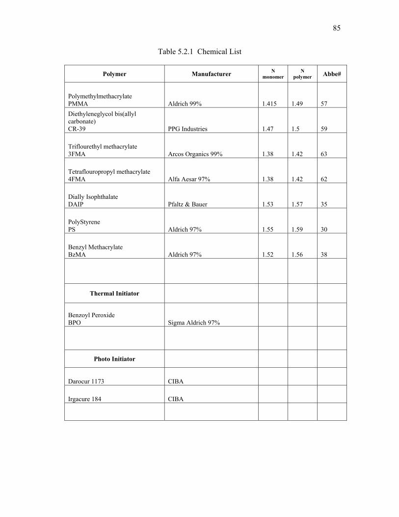
85

Table 5.2.1 Chemical List

Polymer Manufacturer N monomer

N polymer Abbe#

Polymethylmethacrylate PMMA Aldrich 99% 1.415 1.49 57 Diethyleneglycol bis(allyl carbonate) CR-39 PPG Industries 1.47 1.5 59

Triflourethyl methacrylate 3FMA Arcos Organics 99% 1.38 1.42 63

Tetraflouropropyl methacrylate 4FMA Alfa Aesar 97% 1.38 1.42 62

Dially Isophthalate DAIP Pfaltz & Bauer 1.53 1.57 35

PolyStyrene PS Aldrich 97% 1.55 1.59 30

Benzyl Methacrylate BzMA Aldrich 97% 1.52 1.56 38

Thermal Initiator

Benzoyl Peroxide BPO Sigma Aldrich 97%

Photo Initiator

Darocur 1173 CIBA

Irgacure 184 CIBA

86

5.3 Polymer GRIN diffusion exchange method

There are several methods for obtaining gradient index copolymer blends.

The most common are interfacial-gel copolymerization [5.1] (a.k.a. swollen-gel

polymerization[5.2]), photo-copolymerization [5.3], centrifugal field [5.4], and diffusion

exchange [5.5]. Diffusion exchange is the most common practice and is the method used

in this thesis.

The gradient index profile is a continuously varying composition of high index

polymer to low index polymer. The refractive index n of combining M1 and M2

monomers relates to the Lorentz-Lorenz equation [5.6],

22

2

22

121

21

2

2

21

21

21 v

nnv

nn

nn

++

+++

=++ (5.1)

where n1, v1 and n2, v2 are the respective indices and molecular volumes of M1 and M2

monomers. A simplified relationship is often used for experimental extrapolation.

2211 vnvnn += (5.2)

Wu and Koike [5.7] have shown experimentally that both equations are acceptable, and

in fact equation 5.2 fit their experimental plots slightly closer. The liquid monomer

diffusion exchange process creates a continuously changing ratio v1 to v2 of the two

monomers inside a partially polymerized matrix of monomer M1.

The process of diffusion exchange is essentially a three step process. The first

step is pre-polymerization, where the primary monomer M1 is partially polymerized. The

partially polymerized monomer is a matrix of linear, branched, and networked polymers

87

that is able to hold the shape of the final polymer element, but still contains a large ratio

of monomer. This state of polymerization is often referred to as the ‘gel stage’. The

second step is diffusion. In this step, the secondary monomer M2 undergoes a diffusion

exchange process replacing some monomer in the partially polymerized gel. The

diffusion of secondary monomer into the gel creates a concentration distribution that

defines the gradient index profile. The diffusion exchange can take place in liquid or

vapor [5.8] monomer bath. The third and final step is to fully polymerize the system.

The copolymerization of the gel with the inter-diffused monomer is achieved through a

final thermal or photo curing process.

There are a few general rules of thumb for the diffusion exchange method. To

obtain clear polymers, the monomers must be completely miscible in the ratios used. To

achieve a large ∆n, the primary and secondary polymers must have a large difference in

refractive index. Note in table 5.2.1 that many monomers undergo large changes in index

when polymerized, and the polymer, not monomer, index of refraction is relevant. Linear

and branched partial polymerizations do not hold their shape, a high degree of networked

chains are required in the partial polymerization stage. Primary monomers are often

chosen based on their ability to hold their shape in gel form at very low conversion ratios,

the ratio of polymer to monomer. More monomer in the matrix means more control over

the diffusion exchange process, and higher final ∆n. A monomer with only one double

carbon bond, like MMA, requires a cross-linking agent to allow it to gel at a lower

conversion ratio. Sometimes a third monomer is introduced to improve the conversion

ratio and/or improve miscibility. Other factors that often require consideration when

choosing polymers are; Abbe number (chromatic aberration), stress birefringence,

88

mismatched thermal expansion coefficients, flexibility, elasticity, hardness, and spectral

transmission.

There is a rich background of research on the polymer diffusion exchange process

for GRIN materials. The early history dates back to 1905, when R.W. Wood fabricated

GRIN polymer materials in gelatin with a water and glycerin [5.9]. Naujokas, at Bausch

& Lomb, patented a polymer diffusion process for making multifocus ophthalmic lenses

in 1967 [5.10]. Polymer GRIN research increased in the 1970s with the early growth of

fiber optics. Ohtsuka, at Keio University in Japan, published a paper on fabricating

polymer GRIN rods where the gel stage liquid diffusion technique originated [5.5].

Various techniques and polymer combinations were carried by Ohtsuka, K, and Koike Y

et al. over the years in a collection of papers called “Studies on the Light-Focusing Plastic

Rod.” The works of Iga, et. al. [5.11, 5.12] and Gardner L. R. [5.13], also aided in the

selection of polymers for this thesis and provided a basis for experimental techniques.

The book “Polymers and Polymeric Materials for Fiber and Gradient Optics” is an

excellent resource for the majority of research related to polymer GRIN chemistry and

fabrication [5.14].

89

5.4 Tapered GRIN fabrication

5.4.1 Photo initiated partial polymerization

At the beginning of this research, methods of photo initiated partial

polymerization were attempted. Monomers MMA, CR-39, and, Benzyl methacrylate

were tested with photo-initiators Darocure 1173 and Irgacure 184. Both photoinitiators

have a peak absorbance at ~246,280, and 333nm and were able to polymerize layers up to

4mm thick. An Oriel 200W Hg(Xe) arc lamp (model 66002) is used to activate the

initiators.

The initiated monomer was held in a Teflon chamber between a glass slide and

clear top substrate. The top substrates tested are a clear polyester film ~150um thick and

a flexible elastomer silicone ~200um thick. Methacrylate monomers do leach into

silicone, after a few minutes the smell was noticeable. Methacrylate absorbed in the

silicone can cause warping, but this was only problematic if there was already some slack

in the silicone layer. A copper mask is placed over the substrate layer to block unwanted

UV illumination. Figure 5.4.1 shows the monomer chamber, and figure 5.4.2 shows the

illumination setup. The HeNe beam provides a method to monitor the polymerization. A

lens can be place in the system to create a cone of illumination in the monomer layer.

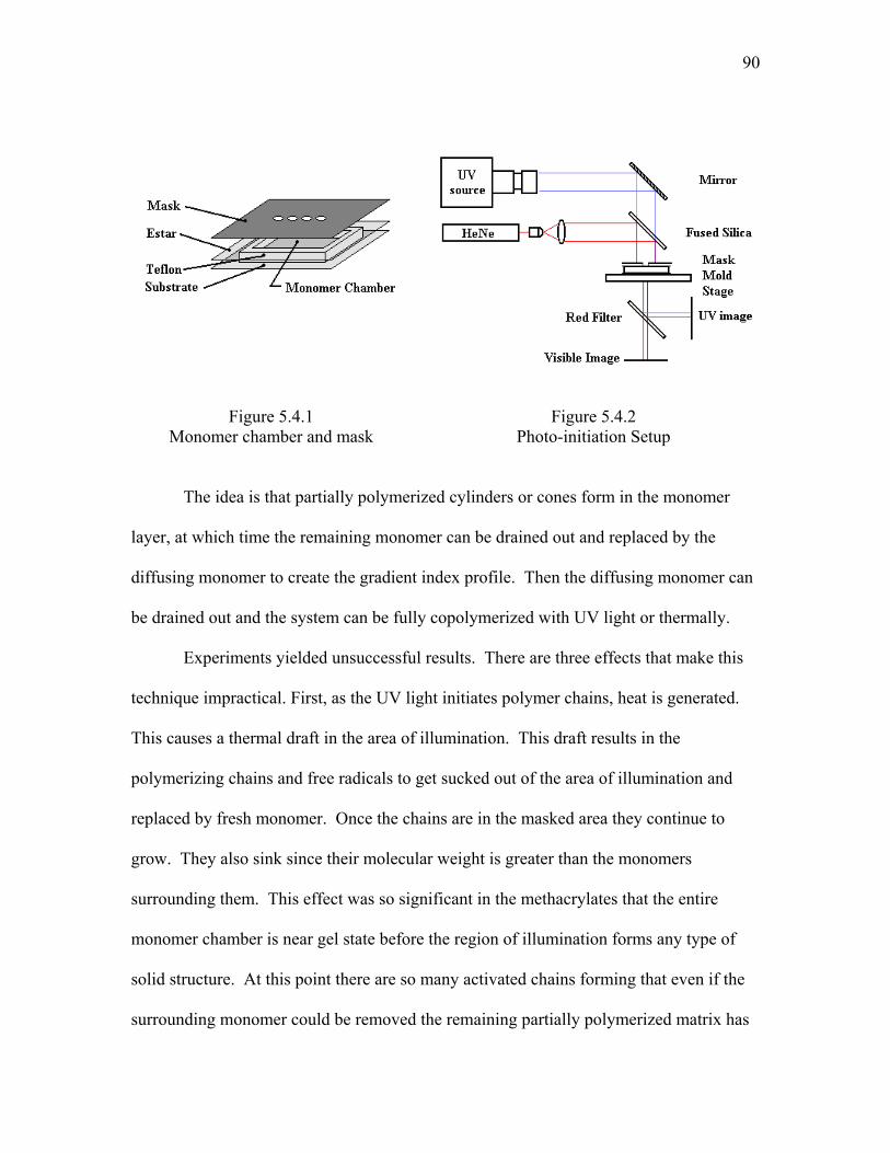
90

Figure 5.4.1 Monomer chamber and mask

Figure 5.4.2 Photo-initiation Setup

The idea is that partially polymerized cylinders or cones form in the monomer

layer, at which time the remaining monomer can be drained out and replaced by the

diffusing monomer to create the gradient index profile. Then the diffusing monomer can

be drained out and the system can be fully copolymerized with UV light or thermally.

Experiments yielded unsuccessful results. There are three effects that make this

technique impractical. First, as the UV light initiates polymer chains, heat is generated.

This causes a thermal draft in the area of illumination. This draft results in the

polymerizing chains and free radicals to get sucked out of the area of illumination and

replaced by fresh monomer. Once the chains are in the masked area they continue to

grow. They also sink since their molecular weight is greater than the monomers

surrounding them. This effect was so significant in the methacrylates that the entire

monomer chamber is near gel state before the region of illumination forms any type of

solid structure. At this point there are so many activated chains forming that even if the

surrounding monomer could be removed the remaining partially polymerized matrix has

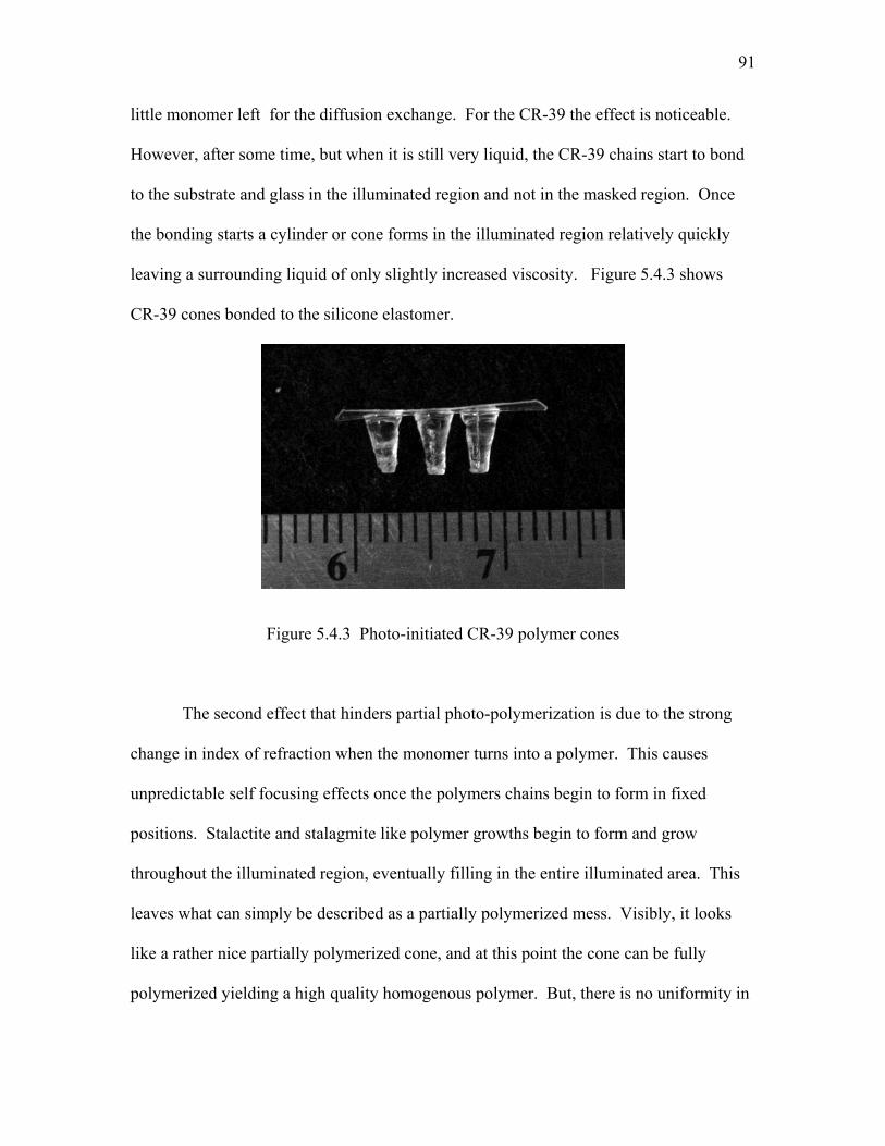
91

little monomer left for the diffusion exchange. For the CR-39 the effect is noticeable.

However, after some time, but when it is still very liquid, the CR-39 chains start to bond

to the substrate and glass in the illuminated region and not in the masked region. Once

the bonding starts a cylinder or cone forms in the illuminated region relatively quickly

leaving a surrounding liquid of only slightly increased viscosity. Figure 5.4.3 shows

CR-39 cones bonded to the silicone elastomer.

Figure 5.4.3 Photo-initiated CR-39 polymer cones

The second effect that hinders partial photo-polymerization is due to the strong

change in index of refraction when the monomer turns into a polymer. This causes

unpredictable self focusing effects once the polymers chains begin to form in fixed

positions. Stalactite and stalagmite like polymer growths begin to form and grow

throughout the illuminated region, eventually filling in the entire illuminated area. This

leaves what can simply be described as a partially polymerized mess. Visibly, it looks

like a rather nice partially polymerized cone, and at this point the cone can be fully

polymerized yielding a high quality homogenous polymer. But, there is no uniformity in

92

the partial polymerization, and diffusion into a randomly varying polymer matrix results

in a randomly varying and pretty much useless gradient index profile. This is a

somewhat ironic problem since self focusing is also used effectively for making micron

sized artificial apposition cones in homogeneous polymers [5.15].

The third effect results from UV absorption in the polymer. The UV initiators

used to start the polymerization are also strong UV absorbers. The polymerizing chains

that have leftover UV initiator remnants absorb significantly more UV light than the

liquid monomer. The increased absorption increases the local reaction rate and adds a

little more heat to compound the polymerization. This causes any area that begins to

form a partially polymerized matrix to reach full polymerization at an accelerating rate.

It also cuts down on UV light that penetrates further into the illuminated area, slowing the

polymerization rate further from the source. The result is that the cones in figure 5.4.3

are completely polymerized at the top, and have just reached gel state at the bottom.

Although this method proved impractical for photo partial polymerization,

alternate methods can still be explored. Self focusing and absorption effects are

significantly reduced when diffuse illumination is used. A transparent or translucent

mold filled with initiated monomer may yield better results. But since this still requires

removal of the partially polymerized cones from the mold to be placed in the secondary

monomer, it is not any different from the standard thermal polymerization technique

which yields much more favorable results

93

5.4.2 Liquid diffusion thermal copolymerization method

Figure 5.4.4 diagrams the steps for fabricating tapered gradient index cones by the

liquid diffusion exchange process. First the monomer is mixed with a thermal initiator.

Second, once the initiator is fully dissolved, the monomer is poured and sealed into the

tapered mold, and then placed in a thermal bath to begin polymerization. Third, when a

stable gel stage is reached it is carefully removed from the mold. Fourth, the gel is

placed in a liquid monomer bath for the diffusion exchange. Finally, when the monomer

has diffused to the desired concentration profile, it is place back in the mold and into an

oven to fully copolymerize the gel and monomers. The following section details each

step with enough detail for the experimental process to be recreated.

HEAT

HEAT

1. 2. 3. 4. 5. Monomer

preparation Partially

polymerize Remove from

mold Monomer diffusion

Fully polymerize

Figure 5.4.4 Process diagram

94

1. Monomer Preparation

All monomers and initiators are used as purchased. No distillation, purification,

drying, removal of inhibitors, or re-crystallization is performed. The primary monomer

M1 is measured by weight into a test tube. The thermal initiator Benzoyl peroxide BPO

is added to the monomer to the amount of 3% by weight. The mixture is placed in a 50oC

water bath and agitated for 10 minutes until the initiator is completely dissolved. Dry

nitrogen is then bubbled through the mixture for 5 minutes to remove oxygen and

moisture.

Polypropylene pipette tips are used for the tapered cylindrical mold. These are

available in many sizes and tapers, are clear or translucent for viewing, thermally stable,

non reactive to monomers, and both the gel state and fully polymerized cones are easily

extracted. They sometimes come with caps, and are compatible with the rubber septa

caps used. The tip is sealed shut with a ~1mm bead of quick setting or UV curing epoxy.

The top is capped with a septa and the empty chamber filled with dry nitrogen to remove

oxygen and moisture. A syringe is then used to transfer the initiated monomer into the

mold. The mold is filed ~1cm past the tapered region of the pipette. This is to ensure

that during the liquid monomer diffusion exchange any diffusion that may occur at the

top of they partially polymerized cone has little to no effect on the gradient index profile

in the tapered region. A few circular spins with the tip outward gets rid of any bubbles in

the tapered region.

The liquid diffusion monomer M2 is prepared in another test tube. It is also used

as purchased. For the experiments in this thesis it was not necessary to add additional

thermal initiator to M2. There is still enough initiator in the M1 gel to fully copolymerize

95

the system after diffusion. The monomer is bubbled with nitrogen for 5 minutes before

the diffusion, and an additional two minutes after the M1 gel is placed in the M2

monomer.

2. Partial polymerization

An MGW Lauda K20 water bath is used for thermal partial polymerization. This

keeps the mold thermally stable (±0.5oC) at temperature T1 for a partial polymerization

time of t1. A temperature controlled bath is crucial so that it can also keep the polymer

cool. The process of polymerization generates heat on its own and if the heat is not

dissipated rapid polymerization can occur. This can result in unpredictable

polymerization times, bubbles in the polymer, and a potentially violent reaction. The

mold is placed in a secondary water filled container inside the bath as a precaution, and in

case some monomer leaks out of the mold. The mold must be almost completely

submerged in the bath in order to avoid any thermal gradient. Attempts were made to

polymerize a spring of wire inside the top of the system that would make it easier remove

the polymer from the mold, but having the spring or even just the cap out of the water

bath results in top section being significantly less polymerized than the tapered section.

96

3. Removal from mold

Once the monomer reaches the desired ‘gel state,’ the mold needs to be cooled. It

is desirable to cool the mold as quickly as possible to dissipate heat being generated in

the system and stop polymerization. If the gel is elastic, this can be done very quickly in

cool water or even an ice bath, but for some polymers the stiff gel is very fragile and

sensitive to thermal shock. In early experiments to test partial polymerization times (t1),

occasionally the partially polymerized CR-39 and DAIP fractures internally during

cooling. This only happened in glass test tubes, not the polypropylene pipettes, and was

likely do to stronger adhesion to the glass surface. Allowing it to cool for 5 minutes in a

warm tap water bath prevented this.

Once the gel is cooled it can be removed from the mold. First, the bottom of the

pipette is cut off with a razor blade just above the epoxy. Then the cap is removed.

Gentle pressure on the sides of the mold, and poking at the rim of the gel aids in

loosening the gel from the mold. If this does not begin to loosen the gel, a razor blade is

used to cut the mold down to just above the top of the gel. Caution is taken not to tear or

cut the gel. Even small nicks in the gel can grow during the diffusion process and ruin

the sample. A technique that works consistently is to first dab the top and bottom of the

mold with a small amount of monomer M2 that acts like a lubricant between the gel and

the mold. Then a gentle amount of compressed air or nitrogen is released into the tip of

the pipette pushing the gel out of the mold. The gel is delicate and very slippery. As it

comes free of the mold, it is transferred using a small test tube.

97

4. Monomer diffusion

Figure 5.4.5 M1 Partially polymerized gel suspended in M2 liquid monomer.

Septa

Wire holder

M1 Gel

M2 Monomer

Figure 5.4.5 is a diagram of the M1 gel suspended in the M2 monomer. The gel is

suspended in the monomer with the top of the cone just above the surface of the liquid.

The test tube is capped with a septa and purged with nitrogen. The wire holding the gel

pokes through the septa so the height can be adjusted. To hold the gel in place, it worked

best to carefully penetrate the top portion of the gel with thin wire. The gel is very

slippery in the monomer, and can swell making clamping or tying very difficult. The gel

occasionally broke where the wire penetrated it. Fully submerging the gel and letting it

rest on the bottom can work as long as it is moved fairly often, or can sit on end. Lying

on the same side too long will inhibit diffusion at that boundary resulting in a profile that

is not symmetrical.

98

The M2 monomer is diffused into the M1 gel at temperature T2 for time t2. For

higher temperatures the diffusion chamber is placed in another water bath to maintain a

constant temperature.

5. Full copolymerization

After the diffusion process the gel is then placed back in the original mold.

Returning it to the mold helps prevent, or deter monomer from diffusing or evaporating

back out of the gel. Placing the gel back in the mold also leaves a clear and smooth outer

surface on the fully polymerized sample. When some of the monomer diffuses back out,

the gradient index near the edge will start to return back to the M1 index of refraction.

This can create wings on the edge of the profile, see figure 5.4.6. This is a well

documented phenomenon [5.5]

Figure 5.4.6 An ideal GRIN profile after diffusion in grey, and after evaporation in black.

If the final polymerization stage involves higher temperatures, for monomers with lower

boiling points it is more likely evaporation has a significant affect. Evaporation can even

result in getting the inverse of the desired GRIN profile. The DAIP-MMA tapered GRIN

experiments in this thesis came very close to such an outcome (see chapter 6). Photo

99

initiated polymerization is not used for the final copolymerization in this thesis, but it

may provide a way to avoid evaporation effects due to high temperature final

polymerizations.

Once the gel is back in the mold, it is placed in a test tube, sealed and purged with

dry nitrogen. It is then placed in an oven at temperature T3, for time t3 to allow it to fully

copolymerize. After time t3, it is best to remove the copolymer from the mold and leave it

out in the oven for a few hours to allow any remaining monomer trapped inside to

evaporate.

5.4.3 Process control of GRIN profile

Generating the optimal gradient index profile in polymers is non-trivial. Now that

the reader is provided the basic chemistry and experimental procedure, it is easier to

discuss the variables that govern the final GRIN profile.

Fick’s second law of diffusion [5.16],

⎟⎟⎠

⎞⎜⎜⎝

⎛∂∂

+∂∂

+∂∂

=∂∂

2

2

2

2

2

2

zC

yC

xCD

tC ; (3)

states that the rate of diffusion ∂C/∂t depends on the concentration gradient and the

diffusion coefficient D (t is time, and x, y, and z are Cartesian coordinates). The

concentration profile at a given time is easiest to predict model when D is constant, as

well as any boundary conditions, and the initial concentration is uniform. However, due

to a combination of material properties and inherent compounding affects in the

fabrication method, the diffusion constants are highly variable and making the desired

GRIN profile becomes a qualitative process [5.17].

100

The shaping of the GRIN profile can be divided into three periods. The first

period occurs during the partial polymerization of monomer M1. Uniform polymerization

of the monomer yields a constant concentration and diffusion coefficient. Thermal

gradient will create non-uniform polymerization and are usually the result of

polymerizing too quickly, or by not maintaining a constant temperature. If significant

networking of the polymer does not occur, gravity can also create a non uniform gel.

Polymer chains can be significantly heavier and will sink, resulting in a gel that is more

polymerized at the base. This is an argument for keeping the partial polymerization stage

as short as possible. Also, increased networking of the chains significantly reduces this

gravitational gradient.

The second period is during the monomer diffusion stage. As M1 monomer

diffuses out of the gel, it is changing the external concentration of M2 monomer that is

diffusing into the gel. Typically, the volume of M2 monomer is several times greater than

the gel so that the diffusion rate at the boundary is effectively constant. Polymerization is

still continuing to some degree during the diffusion stage. At room temperature this is a

negligible amount. Therefore the diffusion coefficient of the M1 gel is more likely to be

constant aside from any chemical reaction effects (some monomers are highly reactive

and can break down the gels matrix over time if energy is not provided to initiate

polymerization). At higher temperatures the diffusion rate is faster. Samples of equal

size in this thesis have diffusion times that vary from 5 min at 80oC to >10 hours at room

temperature. But, at higher temperatures polymerization may continue fast enough that

the diffusion coefficient varies significantly with time, directly affecting the GRIN

profile.

101

The final period is after the gel is removed from the monomer. As mentioned

early, evaporation can affect the concentration profile, most significantly at the surface of

the sample and at higher temperatures. In addition to that, diffusion is still occurring

within the gel. The concentration profile begins to ‘relax’, as it flattens back out

attempting to reach equilibrium. In order to lock in the desired profile, the

copolymerization typically carried out as quickly as possible to prevent it from relaxing

too much.

5.5 Concluding remarks

Fabrication techniques for making polymer GRIN rods were adopted for making

tapered cylinder GRIN elements. The methods were altered to account for the polymers

used, the profile constraints, and effects unique to the cone geometry. Repeatability of

the procedure is primarily dependant on several factors. The manufacturer of the

chemicals often provides different purities of monomer and can have varying amounts of

inhibitors. Using different initiators or additives, like crosslinking agents, can

significantly change the results. Oxygen, moisture, and other environmental effects can

be controlled to much stricter requirements than those used in this thesis and may lead to

much higher quality polymers.

The attempts to partially polymerize cones using photoinitiation were

unsuccessful. Achieving both a uniform gel state and symmetrical shape was not

achievable with the process used here. Thermal partial polymerization techniques using

benzoyl peroxide and polypropylene tapered shaped molds produced homogenous gel

102

state cones. Liquid diffusion followed by thermal copolymerization successfully

produced gradient index profiles in the tapered cones, but there were some problems with

monomer evaporating after the diffusion step.

In Chapter 6 the gradient index samples from this fabrication process are

measured and analyzed.

103

References

5.1 Yasuhiro Koike, Yoshitaka Takezawa, and Yasuji Ohtsuka, "New interfacial-gel

copolymerization technique for steric GRIN polymer optical waveguides and lens

arrays," Appl. Opt. 27, 486-491 (1988)

5.2 Lieu J., Liu H., “Preparation of gradient refractive index rod by swollen-gel

polymerization,” Polymer, V. 38, No. 5, 1997

5.3 Ohtsuka, Y., Yamamoto N., “Light-Focusing plastic Rod Prepared by

Photocopolymerization of Methacrylic Esters with Vinyl Benzoates,” Applied

Physics Letters 29, no. 9, 559-561, 1976

5.4 Hamblen, D., “Method for Making a Plastic optical Element Having a Gradient

Index of Refraction,” U.S. Patent no. 4,022,855 (assignee: Eastman Kodak Co.,

10 May 1977)

5.5 Ohtsuka, Y., “Light-Focusing Rod Prepared from Diallyl Isophthalate-Methyl

Methacrylate Copolymerization,” Applied physics Letters 23, no. 5, 2547-248,

1973

5.6 Y. Koike, "Graded index materials and components," in Polymers for Lightwave

and Integrated Optics, L. A. Hornak, ed. (Dekker, New York, 1992), Chap. 3, pp.

71–104.

5.7 Shang Pin Wu, Eisuke Nihei, and Yasuhiro Koike, "Large radial graded-index

polymer," Appl. Opt. 35, 28-32 (1996)

104

5.8 Yasuji Ohtsuka and Toshiko Sugano, "Studies on the light-focusing plastic rod.

14: GRIN rod of CR-39—trifluoroethyl methacrylate copolymer by a vapor-phase

transfer process," Appl. Opt. 22, 413-417 (1983)

5.9 Wood, R. W., Physical Optics, 3rd ed (Macmillan: New York, 1934) 88-90

5.10 Naujokas, A. A., Multifocal Opthalmic Lens, U.S. Patent no. 3,485,556 (assignee:

Bausch and Lomb Co.,) 1967

5.11 Iga, K., et al., “Optimum Diffusion Condition in the Fabrication of a Plastic

Lenslike Medium,: Applied Physics Letters 26, no.10 (1975) 578-579

5.12 Iga, K., and Yamamoto N., “Plastic Focusing Fiber for Imaging Applications,”

Applied Optics 16, no. 5 (1977) 1305-1310

5.13 Gardner, L., “Studies in Gradient Index Polymer Materials,” Doctoral Thesis,

University of Rochester, 1989

5.14 Lekishvili N., Nadareishvili L., Zaikov G., Kanashvili L., Polymers and

Polymeric Materials for Fiber and Gradient Optics, New Concepts in Polymer

Science 12, VSP, 2002

5.15 K. Jeong, J. Kim, L. Lee “Biologically Inspired Artificial Compound Eyes,”

Science 28, Vol. 312. no. 5773, pp. 557 – 561, 2006

5.16 Crank J., The Mathematics of Diffusion, 2nd ed., Oxford University Press,

London, 1975, chapter 1.

5.17 Ohtsuka Y., Sugano T., Terao Y., “Studies on the light-focusing plastic rod. 8:

Copolymer rod of diethylene glycol bis(allyl carbonate) with methacrylic ester of

fluorine containing alcohol,” Applied Optics, V. 20, No. 13, 1981

105

Chapter 6

Polymer Tapered Gradients

Preparation and Analysis

6.1 Introduction

This chapter examines the final polymer tapered gradient samples. Sample

preparation and measurement techniques are detailed. Gradient index profiles are

measured using a Mach-Zehnder interferometer and a novel method for determining

the absolute index is also presented. The DAIP CR-39 copolymer produces a

gradient index profile similar to proposed index profiles in chapter four. The

measured profile is imported into CodeV and compared to the standard tapered radial

profiles. The profile is also compared to a Fickian diffusion model.

6.2 Tapered GRIN samples

Dially Isophthalate (DAIP, n = 1.57) is the primary high index polymer M1

used in this thesis, and diethyleneglycol bis ally carbonate (CR-39, n = 1.5) is the

secondary low index monomer M2. Samples of DAIP (M1) with MMA (methyl

methacrylate, M2), and CR-39 (M1) with 3FMA (triflourethyl methacrylate, M2), have

been made, but the DAIP/CR-39 combination is favorable for fabrication and also

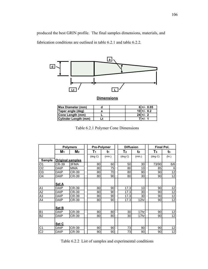
106

produced the best GRIN profile. The final samples dimensions, materials, and

fabrication conditions are outlined in table 6.2.1 and table 6.2.2.

Max Diameter (mm) d 6 +/- 0.05Taper angle (deg) a 10 +/- 0.2Cone Length (mm) L 24 +/- 2Cylinder Length (mm) Lt 7 +/- 1

Dimensions

d

a

Lt L

Table 6.2.1 Polymer Cone Dimensions

M1 M2 T1 t1 T2 t2 T3 t3(deg C) (min.) (deg C) (min.) (deg C) (hr.)

Sample Original samplesO1 CR-39 3FMA 80 60 50 30 73/90 6/6O2 DAIP MMA 80 75 80 10 85O3 DAIP CR-39 80 70 80 90 90 12O4 DAIP CR-39 80 90 80 30 90 12

Set

6

AA1 DAIP CR-39 80 90 17.3 10 90 12A2 DAIP CR-39 80 90 17.3 30 90 12A3 DAIP CR-39 80 90 17.3 30 90 12A4 DAIP CR-39 80 90 17.3 12hr 90 12

Set BB1 DAIP CR-39 80 80 30 17hr 90 12B2 DAIP CR-39 80 80 30 17hr 90 12

Set CC1 DAIP CR-39 80 90 73 90 90 12C2 DAIP CR-39 80 90 73 90 90 12

Polymers Pre-Polymer Diffusion Final Pol.

Table 6.2.2 List of samples and experimental conditions

107

Figure 6.2.1 is a collection of photographs of a fully polymerized tapered

gradient index cone (sample B1). A) is the final cone as removed from the mold. B)

is after the ends are cut and polished. C) shows the quarter pitch of the cone as

collimated laser beam comes to a focus inside the sample. In D), the small end of the

cut and polished cone is placed against a ruler, and the image through the top of the

cone shows magnified and inverted one millimeter tick marks.

A)

B)

C)

D)

Figure 6.2.1 The scale in D) seen through the cone is in millimeters.

All images are scaled equally.

108

6.3 Sample Preparation

The gradient index profile in the tapered cones is measured using

interferometry. This requires cutting the samples into thin (~500μm) flat slices. The

stronger the ∆n of the sample the thinner it needs to be in order to resolve fringes.

The equation that relates the change in refractive index to fringes in the

interferograms is:

d

Nn λ=Δ , (6.3.1)

where N is the number of fringes, λ is the wavelength of the source, and d is the

thickness. The accuracy of the measurement can be adversely affected by variations

in sample thickness. The accuracy of the phase measurement in the interferometer is

related to error in the thickness:

( )nd

ndΔ−Δ

=Δ 1φφ , (6.3.2)

where φ is the phase, φΔ is the phase error, d is the sample thickness, Δd is the error

in the sample thickness, n is the base index of the sample, and Δn is the change in

index. This relationship shows the sample should be thick relative to the surface

error, but if it is too thick, it is not possible to resolve the fringes in the image. Take

an example gradient index sample with thickness d = 500μm, N0 = 1.57, and ∆n =

0.03, that has a 5μm surface error. This is approximately 5 waves of error (at

632.8nm), resulting in a ~20% error in the measurement of ∆n. Not only is this an

unacceptable amount of error for measuring any detail, but thin slices of polymer are

109

soft and flexible, and cutting and polishing both sides of a sample to achieve better

than five microns of thickness error is a daunting task. To improve the accuracy of

the measurement without going to great lengths to make the samples flat, they are

measured in a flat optical cell while immersed in an index matching fluid or optical

epoxy instead of air. This changes equation 6.3.2 to read:

ddΔ

≈Δφφ . (6.3.3)

This reduces the error by (n-1)/ ∆n. Under the same conditions in the previous

example, the error is now ~1%. This significantly relaxes the constraints on cutting

and polishing the sample. A goal for ten microns of thickness error is much more

realistic for the sample preparation techniques used here.

Figure 6.3.1 The GRIN cone is sectioned and mounted in an index matching optical epoxy

between two glass slides.

Slices are made perpendicular and parallel to the cone’s axis of symmetry (see

figure 6.3.1) using a Buehler Isomet diamond saw. Distilled water with liquid soap is

110

used as a lubricant. The soap is added to prevent jamming by stopping the residual

polymer from clogging the blade. The two cuts required for each section are always

made consecutively to ensure parallel faces. Cuts that are not parallel introduce

wedge into the sample that can interfere with the GRIN profile measurement.

The slices are then polished to smooth out marks from the saw blade and

jagged edges. Left over saw marks and scratches after polishing are typically only 1

or 2 microns deep. Glassy surfaces are not necessary for measurement as the pieces

are mounted in index matching epoxy. Polishing is kept to the bare minimum. The

thin pieces are flexible and soft compared to glass and tend to polish unevenly. GRIN

polymers are particularly difficult to obtain a high quality polish because the two

materials often have different removal rates. Over polishing the pieces can cause

rounding of the edges, surface roll, or introduce an uneven wedge. These effects are

much worse relative to saw marks and scratches, since they add a broad unpredictable

variation to the samples thickness. Loosing some fringe quality to saw marks and

surface defects is favorable if it keeps the sample surfaces uniformly flat.

Samples are polished using Thorlabs aluminum oxide lapping pads in the

order 5μm, 3 μm, 1 μm, and 0.3 μm grit with distilled water as a lubricant. Samples

that are mounted in index matching epoxy only need the 1 μm grit polish. Avoiding

the larger grits significantly reduces edge roll off. An ultraviolet curing optical epoxy

Norland® 63 (n = 1.56) is used to mount the sample sections between two glass

slides. For liquid index matching the samples are placed in 1mm Starna optical cells.

The image in Figure 6.3.1 shows the epoxy mounted sections A, B, and C from a

111

tapered polymer GRIN. A is a 5mm radial section, C is a 3mm radial section, and B

is the Xmm cross section between A and C.

To measure error in the GRIN profile measurements due to sample thickness

variation a homogeneous slice of polymethyl methacrylate (PMMA n = 1.49) is

prepared in the same manner as the GRIN samples (see Figure 6.3.2). It is mounted

in Norland 63 between two glass slides and placed in the interferometer. There is

slightly less than 1 wave of error near the edge from roll off, and there is also some

error from a small saw wedge in the lower right hand quadrant. The wedge occurs

sometimes if the saw blade begins to flex near the end of a cut. The effect is small,

and if it is noticeable, the area can be avoided when collecting the profile data. The

saw direction can also be marked on the edge of the sample with a notch or

permanent mark.

Figure 6.3.2 Homogeneous sample of PMMA shows error in sample thickness is less than one wave. Sample is outlined in the dotted line. The arrow indicates sawing direction

112

The index change in this measurement is ~0.08 and the wavelength is 632.8nm

(HeNe). Using equation 6.3.1, one fringe yields sample thickness variation of around

8 microns, and this is mostly around the very edge and the wedge. This concludes

that for 500μm samples the profile measurements are accurate to 2% error or better.

Note that there are some tilt fringes in the surrounding epoxy, which imply that the

two surfaces are not perfectly parallel, and adjusting the mirror in the reference arm

will compensate for this error.

6.4 Interferometer and Data Processing

Figure 6.4.1 Mach-Zehndar interferometer used for GRIN profile measurments.

The gradient index profile of a sample is measured with a Mach-Zehndar

interferometer diagramed in figure 6.4.1. Figure 6.4.2 shows a set of interferograms

from sections A, B, and C of a tapered GRIN.

113

A B C

Figure 6.4.2 Interferometer images of tapered GRIN sections. The white bar is ~1mm.

It is normal to have a small amount of wedge between the glass slides in the index

matched layer. Wedge can cause some confusion when dealing with tilt fringes. The

fringe pattern in samples with wedge appear decentered within the bounds of the

sample. Most of the wedge is eliminated by using a spacer of uniform thickness

between the slides, or using a good quality glass optical cell.

Originally, since the samples are very flat, the glass slides were tightly pressed

down onto the samples, but this is not recommended. This appeared to work well

until about a week or two later when the samples where viewed again. Squiggly air

gaps began to appear around the edges of the samples that slowly crept inwards (see

figure 6.4.3). The cause of this is likely due to strain in the sample and/or in the thin

epoxy layer between the sample and the glass. The sample has strain in it from the

pressure applied when pressing the slides together. The epoxy has strain from any

shrinkage during curing and pulls between the sample and the glass.

114

Figure 6.4.3 Air gaps creeping inwards as the index matching epoxy fails.

Even significant wedge of several waves of error does not present a problem if the

samples are prepared well. Since the change in index of refraction at the boundary of

the sample is constant on the entire diffusing surface the argument can be made that

in a flat sample the fringes at the edge of a diffusion boundary will always parallel

that edge. This fact makes it a straight forward process for using the reference arm

mirror to compensate for any wedge. There are two cases when this is not valid and

an alignment can not be found where the fringes are continuously parallel to the edge

at a diffusion boundary. The first case is when there are several waves of error due to

non uniform thickness. The can happen if the sample is polished unevenly. The

second case is mentioned in chapter five, when during the diffusion stage a diffusing

surface comes in contact with the edge of the container, retarding the diffusion in that

area. This causes the gradient index profile to become lopsided, see figure 6.4.4.

115

Figure 6.4.4 Lopsided diffusion. The left side of the sample was in contact with the edge of the container during the diffusion stage.

The GRIN profile is measured for several cross sections of the interferograms,

usually across the diameter of a radial slice, and along the central axis of the cone.

Using ImageJ public domain image processing software, the pixel amplitude

information of a cross section is sampled and the data imported into MATLAB®.

Using equation 6.3.1, each fringe represents a discreet change in the index of

refraction. In MATLAB®, the sinusoidal intensity pattern is unwrapped and fit to a

4th or 6th order polynomial to generate the gradient index profile (figure 6.4.5a). Then

the data is rescaled to the correct dimensions and index change (figure 6.4.5b). .

116

Figure 6.4.5 a)

Gradient Index Profile

0

0.005

0.01

0.015

0.02

0.025

0.03

0.035

-2.5 -2 -1.5 -1 -0.5 0 0.5 1 1.5 2 2.5

Radius (mm)

Inde

x Ch

ange

(Δn)

Figure 6.4.5 b)

Figure 6.4.5 a) Raw data unwrapped in Matlab, and residual from curve fit. b) Final correctly scaled GRIN profile measurement.

0 200 400 600 800 1000 1200-2

-1

0

1

2residuals

0 200 400 600 800 1000 1200

0

10

20

30

40

50

y = - 6.8*z4 + 0.85*z3 - 18*z2 + 0.83*z + 51where z = (x - 6.4e+002)/5e+002

117

6.5 Absolute index measurement of a GRIN material

The interferograms provide accurate profile of the change in the index of

refraction, but they do not give any information about the absolute index. If a

homogeneous region of the polymer is available it can be used as a reference point

when the homogenous index is known, but unless the sample is under diffused it will

no longer have a homogenous region. For measuring the absolute in a sample with a

fully diffused gradient index profile index, there are chemical analysis methods

[6.1,6.2], and optical methods [6.3,6.4]. Those techniques are often destructive or

have a large margin of error.

An alternate technique has been developed in this thesis where reference

points on the sample are found that match the index of the surrounding medium.

Only one matching point is necessary and then the index of refraction at any point on

the sample can be extrapolated from the profile measurement, or multiple

measurements at different indices can be used to confirm the accuracy of the profile

measurement. The technique also uses same interferometer and sample preparation

method.

The measurement is made on an edge of the sample that exposes the gradient

index profile. For sections of type B, it can be made at either of the cut ends. Radial

sections, type A and C, are cut in half so the profile is exposed across the diameter.

The sample is placed in an optical cell and immersed in an index matching fluid that

has an index somewhere within the gradient index profile. The cell is then placed in

the interferometer and held at a steep angle that exposes the edge to be measured. An

angle in the range of 30-45 degrees was adequate and does not affect the result.

118

Light traveling through most of the sample is unaffected, just a small shift due

to change in optical path length from tilting the sample. However, the edge is no

longer a sharp boundary. It is shaped like a prism now, a region where the gradient

index profile tapers down to zero thickness. The position where the index of the

sample matches the index matching fluid is found by observing the behavior of the

fringes in the prism shaped region. A fringe represents a path through the sample,

cell, and index matching fluid that has equal optical path length. When a fringe in the

sample reaches the prism region, it has to follow a path of equal path length and three

things can happen. If the fringe is following a path where the index of the sample and

index matching fluid are the same, it continues straight through because the change in

thickness does not matter since the indices of the two materials are the same. If the

index of the sample is lower than the fluid, then in the prism region the path straight

to the edge will increase in optical path length. In this case, the path of equal optical

path length curves toward lower index polymer in the sample to balance increasing

volume of higher index fluid. If the index of the sample is higher than the fluid, then

in the prism region, the path straight to the edge decreases in optical path length. In

this case, the path of equal optical path length curves toward a higher index polymer

to balance the increasing volume of lower index fluid. The position where the fringe

does not deviate provides a reference point on the sample with a known index of

refraction equal to the index matching fluid. Figure 6.5.1 illustrates light passing

through the sample, and the behavior of fringes in the prism region on the near the

index matched position.

119

Side View CCD Image

Prism Region

GRIN Sample

Isoindicial surfaces

Light

Figure 6.5.1 Identifying the absolute index of refraction by fringe deviation in an index matching solution.

The index matched positions are unaffected by any errors in the samples

thickness or misaligned tilt in the interferometer, making it and excellent method for

confirming accuracy of the profile measurements. If the profile is to measured at the

same time as the index measurement, the sample must still be prepared to the

accuracy described in the previous section.

A DAIP-MMA sample, that has the evaporation effect causing the index to

rise back up near the boundary, is selected for a test case. The appropriate index

matching fluid should match two positions near the edge to verify that the index does

indeed rise back up. The peak index of the sample should be less than 1.57, the

homogenous index of DAIP, so first the sample is immersed in n = 1.56. The

positions matching n = 1.56 are noted in figure 6.5.2 A. There are ~30 fringes from

120

the left matched point to the left inflection point. Equation 6.3.2 for N = 30, a sample

thickness d = 540 μm, and the wavelength 632.8 nm, gives Δn = 0.035. An index

matching fluid of n = 1.528 is selected that gives Δn = 0.032. It is slightly higher

index so that two index matched positions should be visible near the left edge. The

result is seen in figure 6.5.2 B and in figure 6.5.3.

Figure 6.5.2 A)

Figure 6.5.2 B)

Figure 6.5.2 DAIP-MMA sample. A) immersed in n = 1.56. B) immersed in n = 1.528.

Arrows denote index matched positions.

121

Note that the sample is actually 500 μm thick, but tilted at 36 degrees the path of light

through the sample is ~540 μm. For a Δn of 0.032 equation 6.3.1 gives N = 27.3.

Figure 6.5.3 is a blown up view of the two images side by side that shows how well

the predicted index matched positions line up with the measured positions.

Figure 6.5.3 Side by side comparison of DAIP-MMA sample in two index matching fluids.

n = 1.528 top, n = 1.56 bottom The right most dotted line denotes the position that the high index fluid matched the

index of the sample. The left two dotted lines denote the positions where the low index fluid was predicted to match with the sample.

Index matching fluids used are from Cargille Laboratories. They are accurate to

±0.0002 with a temperature dependence -dn/dT = 4.0*10-4.

These results confirm that using the index matching technique in combination

with the interferograms can produce a quantitative measurement of the index profile.

n = 1.528

n = 1.56~27 fringes

122

6.6 Sample Results

This section examines the copolymer tapered GRIN cones and the gradient

profiles generated for different experimental variants. The DAIP CR-39 copolymer

pair yields gradient index profiles similar to the designs from chapter 4, and the

fabrication process is flexible with few problems. The DAIP MMA and CR-39

3FMA copolymers yielded less favorable results and are more difficult to fabricate

consistently. The following is a brief discussion of issues with copolymers and then

the detailed results of the more successful DAIP CR-39 experiments.

6.6.1 DAIP - MMA

The DAIP MMA pair can produce a change in index greater than 0.03 , and

has the shortest diffusion time. It also suffers from significant evaporation and slight

warping during the full polymerization. The warping is due to the fact that MMA

shrinks almost 30% during polymerization. The evaporation is considerable due to

the higher temperature required for full polymerization of DAIP. Figure 6.6.1 show

the effects of evaporation in a sample not placed back in the mold for full

polymerization.

123

Figure 6.6.1 Section B of a DAIP MMA cone. The interferogram shows severe effects from evaporation of MMA monomer during final polymerization.

An interesting outcome of the strong evaporation effect is that the GRIN

profile starts off having positive power but at the tail end of the cone it has negative

power. This could potentially be a useful process for creating a negative GRIN

element, or used as variable for producing a custom profile. Another positive note is

that the final copolymer has no tinge of yellow that appears in homogeneous samples

of DAIP, and DAIP CR-39 copolymers.

6.6.2 CR-39 - 3FMA

The CR-39 3FMA copolymer is the most difficult to fabricate, and

experiments with this pair have not been continued since the DAIP CR-39 pair

proved to be much more practical. Here are few points on the problems with this

copolymer pair. When CR-39 is used as the primary monomer M1, it is very sensitive

to the temperature and the amount of thermal initiator used. The time to gel is

somewhat unpredictable, varying by as much as ten minutes under the same settings

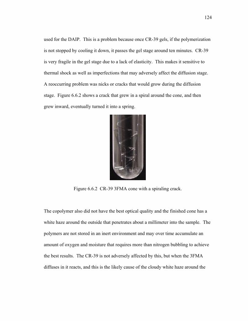
124

used for the DAIP. This is a problem because once CR-39 gels, if the polymerization

is not stopped by cooling it down, it passes the gel stage around ten minutes. CR-39

is very fragile in the gel stage due to a lack of elasticity. This makes it sensitive to

thermal shock as well as imperfections that may adversely affect the diffusion stage.

A reoccurring problem was nicks or cracks that would grow during the diffusion

stage. Figure 6.6.2 shows a crack that grew in a spiral around the cone, and then

grew inward, eventually turned it into a spring.

Figure 6.6.2 CR-39 3FMA cone with a spiraling crack.

The copolymer also did not have the best optical quality and the finished cone has a

white haze around the outside that penetrates about a millimeter into the sample. The

polymers are not stored in an inert environment and may over time accumulate an

amount of oxygen and moisture that requires more than nitrogen bubbling to achieve

the best results. The CR-39 is not adversely affected by this, but when the 3FMA

diffuses in it reacts, and this is the likely cause of the cloudy white haze around the

125

diffusing surface. The 3FMA also suffers from evaporation effects on the GRIN

profile that are comparable to the MMA samples, see figure 6.6.3.

Figure 6.6.3 Half section A of a CR-39 3FMA cone. Index match is visible for n = 1.48. Interferogram shows evaporation effects are significant.

6.6.3 DAIP - CR-39

The DAIP CR-39 copolymer proved to have consistent quality under various

experimental conditions, and produced several gradient index profiles of interest.

Shorter pre-polymerization times, t2, yield a larger change in index Δn, up to 0.046.

Room temperature diffusions take several hours to penetrate into 3mm radius cones.

Results show that complete diffusion with a large Δn is achievable in less than two

hours at higher temperatures, but this also creates a time varying diffusion coefficient

since polymerization continues during diffusion at higher temperatures. GRIN

profiles can vary significantly with increased diffusion temperature. An alternate set

of experiments would need to be developed to quantify these changing diffusion

effects that are also sensitive to the geometry and pre polymerization steps. The

cones do have a less desirable yellow tinge from the DAIP polymer. This may have a

126

simple solution with the proper additives or introduction of a 3rd monomer. The fact

that the DAIP MMA combination is clear suggests that there is likely to be such a

solution. There is no evidence of monomer evaporation or warping in any of the

samples.

Figure 6.6.4 shows a comparison of various sample radial profiles from

DAIP-CR39 experiments. Refer to table 6.2.2 for the list of samples and

experimental conditions.

DAIP CR39Gradient Index Profiles

1.52

1.53

1.54

1.55

1.56

1.57

-3 -2 -1 0 1 2 3

r (mm)

Ref

ract

ive

Inde

x

A1

A2

O4

A4

O3

Sample

Figure 6.6.4 Comparisons of a section A radial profiles (~5mm diameter). Refer to table 6.2.2 for sample experimental conditions.

Room temperature diffusions for times t2 of ten and thirty minutes did not achieve full

diffusion of the monomer into the entire cone (figure 6.6.4 Sample A1 and A2). The

long room temperature diffusion and the diffusions at higher temperatures achieved

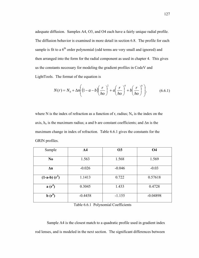
127

adequate diffusion. Samples A4, O3, and O4 each have a fairly unique radial profile.

The diffusion behavior is examined in more detail in section 6.8. The profile for each

sample is fit to a 6th order polynomial (odd terms are very small and ignored) and

then arranged into the form for the radial component as used in chapter 4. This gives

us the constants necessary for modeling the gradient profiles in CodeV and

LightTools. The format of the equation is

( ) ⎟

⎟⎠

⎞⎜⎜⎝

⎛⎟⎠⎞

⎜⎝⎛+⎟

⎠⎞

⎜⎝⎛+⎟

⎠⎞

⎜⎝⎛−−Δ+=

642

0 1)(horb

hora

horbanNrN , (6.6.1)

where N is the index of refraction as a function of r, radius; No is the index on the

axis, ho is the maximum radius; a and b are constant coefficients; and Δn is the

maximum change in index of refraction. Table 6.6.1 gives the constants for the

GRIN profiles.

Sample A4 O3 O4

No 1.563 1.568 1.569

Δn -0.026 -0.046 -0.03

(1-a-b) (r2) 1.1413 0.722 0.57618

a (r4) 0.3045 1.433 0.4728

b (r6) -0.4458 -1.155 -0.04898

Table 6.6.1 Polynomial Coefficients

Sample A4 is the closest match to a quadratic profile used in gradient index

rod lenses, and is modeled in the next section. The significant differences between

128

the three profiles show that the GRIN profile of this copolymer pair has promise for

optimization and controlling higher order aberrations.

The axial behavior of all three samples is nearly identical. Figure 6.6.5 shows

the interferograms of the 3 samples side by side. The slope is close to linear, but

there is a slight increase in fringe density as the radius of the cone decreases, see

figure 6.6.6.

Sample A4 Sample O4 Sample O3

Figure 6.6.5 Section B interferograms of three DAIP CR-39 GRIN cones.

Axial GRIN Profile

1.55

1.552

1.554

1.556

1.558

1.56

1.562

1.564

1 2 3 4 5 6 7 8 9 10

z (mm)

Inde

x of

Ref

ract

ion

Sample A4

Figure 6.6.6 GRIN profile along the axis of DAIP CR-39 sample A4.

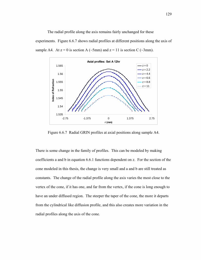
129

The radial profile along the axis remains fairly unchanged for these

experiments. Figure 6.6.7 shows radial profiles at different positions along the axis of

sample A4. At z = 0 is section A (~5mm) and z = 11 is section C (~3mm).

Axial profiles: Set A 12hr

1.535

1.54

1.545

1.55

1.555

1.56

1.565

-2.75 -1.375 0 1.375 2.75r (mm)

Inde

x of

Ref

ract

ion

z = 0z = 2.2z = 4.4z = 6.6z = 8.8z = 11

Figure 6.6.7 Radial GRIN profiles at axial positions along sample A4.

There is some change in the family of profiles. This can be modeled by making

coefficients a and b in equation 6.6.1 functions dependent on z. For the section of the

cone modeled in this thesis, the change is very small and a and b are still treated as

constants. The change of the radial profile along the axis varies the most close to the

vertex of the cone, if it has one, and far from the vertex, if the cone is long enough to

have an under diffused region. The steeper the taper of the cone, the more it departs

from the cylindrical like diffusion profile, and this also creates more variation in the

radial profiles along the axis of the cone.

130

6.7 Performance Comparisons

Figure 6.7.1 illustrates the difference between the radial profile of sample A4

and the quadratic radial profile, the standard for radial gradients.

Sample A4 Profile vs Quadratic Profile of a Radial GRIN

1.535

1.54

1.545

1.55

1.555

1.56

1.565

-2.75 -1.375 0 1.375 2.75r (mm)

Inde

x of

Ref

ract

ion

Radial GRINSample A4

Figure 6.7.1(a) Profile of sample A4 section A, and a best fit quadratic profile.

-0.001

-0.0005

0

0.0005

-2.75 0 2.75r (mm)

Res

idua

l

Figure 6.7.1(b) Residual of 6th order polynomial fit to sample A4 profile.

-0.001

0.002

0.005

-2.75 0 2.75r (mm)

Dev

iatio

n

Figure 6.7.1(c) Deviation of sample A4 profile from a best fit quadratic profile.

131

Table 6.7.1 compares the coefficients that define the radial gradient index profiles

from figure 6.7.1. The N10 quadratic term is very close in both systems, but the

sample still has higher order terms that affect the performance.

N(r) = N00 + N10 r2 + N20 r4 + N30 r6 …

N0 N10 N20 N30

Radial GRIN 1.563 -.0048 - -

Sample A4 1.563 -.00475 -.0002 4.7e-05

Table 6.7.1 Radial coefficients

Figure 6.7.2 compares the measured gradient profile along the central axis (r =

0) of the sample to the sloped and hyperbolic forms from chapter 4, scaled to

equivalent index and geometry values:

Hyperbolic (H-TR GRIN) ⎟⎟

⎠

⎞⎜⎜⎝

⎛+

−−Δ+= 2

2

2

2

0)(1),(

oo

o

hr

zzznNzrN ; (6.7.1)

Linear Sloped (S-TR GRIN) ⎟⎟

⎠

⎞⎜⎜⎝

⎛+

−Δ+=

ooo zz

zzhrznNzrN

)(),( 2

20

0 ; (6.7.1)

where N is the index of refraction as a function of r, the distance from the optical

axis, and z, optical direction, where zo is the apex of the tapered cone, No is the base

index, and ho is the maximum radius, and Δn is the maximum change in index of

refraction.

132

Axial GRIN Profile

1.546

1.548

1.55

1.552

1.554

1.556

1.558

1.56

1.562

1.564

1 2 3 4 5 6 7 8 9 10

z (mm)

Inde

x of

Ref

ract

ion

Sample A4Linear SlopeHyperbolic

Figure 6.7.2 Comparison of tapered GRIN axial profiles.

The measured profiles of the sample are entered into a usergrin file in

CodeV® and compared to a sloped tapered radial GRIN with the quadratic GRIN

profile.

No 1.563 Taper (deg) 5

Δn -0.03 ho (mm) 2.5

Ent. Pupil Dia. 2.5 zo (mm) 28.6

Fields (deg) 0,1.5,3 Wavelength (nm) 632.8

Table 6.7.2 S-TR GRIN Properties in CodeV® model.

133

Third Order Aberrations

-0.16

-0.14

-0.12

-0.1

-0.08

-0.06

-0.04

-0.02

0

0.02

Sphe

rical

Com

a

T As

tig

S As

tig

Dist

ortio

n

(mm

)

S-TR GRIN

SetA12hr

02

46

810

1214

1618

20

F/# EFL(mm) OAL (mm)

S-TR GRIN

SetA12hr

00.050.1

0.150.2

0.250.3

0.35

0.40.450.5

Image h(mm)

Figure 6.7.3 First order properties and third order aberrations of sample A4 (SetA12hr) and a tapered grin with the linear sloped

profile (S-TR GRIN). For a 3 degree field.

The first order properties are closely matched to the S-TR GRIN, but there is

significantly more aberration in Sample A4. Figure 6.7.4 shows the ray aberration

plots for sample A4, and Figure 6.7.5 shows the ray aberration plots for the S TR

GRIN model. Fields are weighted equally, entrance pupil is 2.5 mm, and the image is

at the best focus determined by RMS(root mean square) spot size.

134

Figure 6.7.4 Ray aberration plots for the quarter pitch sample A4

-0.015

0.015

-0.015

0.015

0.00 RELATIVE

FIELD HEIGHT

( 0.000 )O

-0.015

0.015

-0.015

0.015

0.50 RELATIVE

FIELD HEIGHT

( 1.500 )O

-0.015

0.015

-0.015

0.015

TANGENTIAL 1.00 RELATIVE SAGITTALFIELD HEIGHT

( 3.000 )O

135

Figure 6.7.5 Ray aberration plots for the quarter pitch S-TR GRIN

-0.015

0.015

-0.015

0.015

0.00 RELATIVE

FIELD HEIGHT

( 0.000 )O

-0.015

0.015

-0.015

0.015

0.50 RELATIVE

FIELD HEIGHT

( 1.500 )O

-0.015

0.015

-0.015

0.015

TANGENTIAL 1.00 RELATIVE SAGITTALFIELD HEIGHT

( 3.000 )O

136

The ray aberration plots for the S-TR GRIN show third-order spherical

aberration which is standard for a quadratic profile radial GRIN and can be corrected

by adding a 4th order term. The ray aberration plots for sample A4 show significantly

more spherical aberration, and also coma. At the best focus higher order spherical

aberration is providing some balance the third order spherical aberration. Looking

back at figure 6.7.1(a and c) the profiles match very closely, especially the 2nd order

coefficients, but the error contribution of a GRIN medium is proportional to the

optical path length in the GRIN material.

6.8 Diffusion Analysis

Fick’s law defines diffusion in most isotropic materials. This section

compares the measured gradient index profile of sample A4 and compares it to a

Fickian diffusion simulation. Fickian diffusion in a cylinder the diffusion equation

is:

⎟⎠⎞

⎜⎝⎛

∂∂

∂∂

=∂∂

rCrD

rrtC 1

;[6.5] (6.8.1)

where C is the concentration, t is time, r is the radial coordinate, and D is the

diffusion coefficient. This form has a solution for a cylinder of infinite length [6.6].

The geometry and boundary conditions for the diffusion model in this thesis require

numerical solution methods. Comsol Multiphysics® software is used to numerically

simulate Fickian diffusion in the tapered cylindrical geometry.

137

The geometry and boundary conditions for the simulation are based on the

experimental results for sample A4. The diffusion time is 12 hours, the concentration

at the external boundary is zero, and the initial concentration of the cone is .026. A

diffusion coefficient of 0.06 matches the No index of refraction of the simulation to

sample A4 (No is the peak index along the axis of the cone at the 5mm radial diameter

for sample A4). Figure 6.8.1 shows the final concentration in the simulation, scaled

to the index of refraction values, and compares the radial and axial profiles to the

measured data.

Figure 6.8.1 Gradient index profile from a Fickian diffusion simulation. The dotted line indicates the location of the 5mm radius.

Measured vs. Fickian

1.535

1.54

1.545

1.55

1.555

1.56

1.565

0 5 10 15 20

z (mm)

Inde

x of

Ref

ract

ion

Sample A4Fickian Model

Figure 6.8.2 Measured and simulated axial profile.

138

Measured and Simulated Radial Profiles

1.535

1.54

1.545

1.55

1.555

1.56

1.565

-2.75 -1.375 0 1.375 2.75r (mm)

Inde

x of

Ref

ract

ion

Fickian ModelSample A4

Figure 6.8.3 Measured and simulated radial profile.

It is clear that diffusion for CR-39 monomer into partially polymerized DAIP

is very close to the Fickian diffusion simulation. There is still some significant

variation in the shape of the axial profile. Many polymers fall into the category of

pseudo-Fickian [6.7]. This is often the case when the structure is altered by the

diffusant and both the concentration and diffusion coefficient are affected over time.

The shape of the measured data compared to the simulation suggests that the

diffusion coefficient may be decreasing slightly with time. If polymerization is still

occurring during diffusion, even at room temperature, this would cause the diffusion

coefficient to decrease.

139

The simulation only takes into account the profile change from the diffusion

stage. Deviation from the measured data may also be due to effects from the pre

polymerization stage, or the final full polymerization.

6.9 Concluding Remarks

Gradient index copolymers of CR-39 3FMA, DAIP MMA, and DAIP CR-39

were fabricated with the methods described in chapter 5. Sample preparation is

outlined in detail and surface error due to preparation is shown to have a negligible

contribution to the gradient index profile measurements. The radial and axial

gradient index profiles of the samples are measured in a Mach-Zehndar

interferometer. Absolute index measurements of the samples are made with a novel

index matching technique that is also done in the same interferometer.

There were some difficulties with the fabrication of CR-39 3FMA and DAIP

MMA samples, and their gradient index profiles showed that monomer was

evaporating during the final diffusion. The DAIP CR-39 copolymer experiments

produced several unique gradient index profiles, and a change in index of refraction

up to 0.046. The sample with the closest match to the standard quadratic gradient

index profile of GRIN rods is analyzed in detail and modeled in CodeV® The model

is compared to the sloped linear model from chapter 4. The first-order behavior is a

close match, but the deviation from a quadratic profile introduces significant third-

and higher-order spherical aberration.

140

The diffusion profile is also compared to Fickan diffusion simulation. The

profile is close to Fickian, but difference suggests there are other variable effecting

the profile. Pre or post changes to the profile, or a time-dependant diffusion

coefficient.

141

6.10 References

6.1 Yasuji Ohtsuka, “Light-focusting plastic rod prepared from diallyl

isophthalate-methyl methacrylate copolymerization.” Applied Physics Letters,

Vol.23, No 5, 1973

6.2 In-Sung Sohn, Chang-Won Park, “Perparation of Graded Index Plastic optical

Fibers by the Diffusion Assisted Coextrusion Process,” Ind. Eng. Chem Res.,

41, 2002, pg. 2418

6.3 Yasuji Ohtsuka, Yasuhiro Koiki, “Determination of the refractive-index

profile of light focusing rods: accuracy of a method using interphako

interference microscopy,” Applied Optics, Col. 19, Issue 16, 1980

6.4 D. Marcuse, “Refractive index determination by the focusing method,”

Applied Optics, Vol 18, Issue 1, 1997

6.5 Crank J., The Mathematics of Diffusion, 2nd ed., Oxford University Press,

London, 1975, pg 69

6.6 Crank J., The Mathematics of Diffusion, 2nd ed., Oxford University Press,

London, 1975, pg 73

6.7 Crank J., The Mathematics of Diffusion, 2nd ed., Oxford University Press,

London, 1975, pg 255

142

Chapter 7

Summary and Conclusion

Advances in technology continue to discover and duplicate the ways nature

works. This thesis has investigated aspects of compound eyes found on crustaceans

and insects, and made advances in creating ‘bio-inspired’ artificial versions.

Artificial compound optical arrays are still a slowly emerging technology. This is

largely due to the fact that they have the most potential in small sizes, and are less

adaptable to planar geometries. Electronics are continually being miniaturized for

many applications, like the current trend of smaller and lighter portable devices, but

flat is cheap, and compound arrays are still awaiting more development in the fields

of flexible electronics and curved detector arrays. This leaves the research and design

in an awkward space for studying and producing artificial compound arrays, and

work continues on a macro scale that operates equivalent to their much smaller

natural counterparts. The work in this thesis has furthered the research and

development efforts in this level. This chapter provides a summary of the thesis

followed by concluding remarks for future work.

143

The introduction provided a background into natural compound eye designs

and how they differ from simple eyes like in humans. Applications for artificial

versions are discussed as well as current efforts in the field. Research into visual

processing of compound eyes has created a need for optical designs that can produce

specific angular responses.

Chapter 2 then provides the basic principles behind compound array optical

designs and examines how they can be tailored to produces different variations. The

layout of a compound array is defined by a simple set of relationships. These act as a

guide for designing a system of specific size, and resolution. From these

relationships the geometrical parameters of the system are determined, and the limits

and variables can be defined. Two variables, the corneal radius of curvature and the

focal positioning, were selected to illustrate how they can be used adjust the angular

response of ommatidia in an artificial compound array.

Chapter 3 takes the work from chapter 2 and applies it to the design and

fabrication of a prototype system. Apposition and neural superposition designs were

developed and modeled in LightTools®. Their specifications are based on the design

for a high speed object tracking system. The apposition design was selected for

fabrication, and seven and nineteen element prototypes were made. The designed

resolution and overlap in angular response were measured and compared to the

model.

144

The index of refraction provides an additional variable in the design process,

and gradient index elements are common in natural systems. The remainder of the

thesis focused on designing and fabricating gradient index elements for artificial

compound arrays.

Chapter 4 examined the unique GRIN lenses found in natural systems,

specifically those found in the crystalline cones of compound eyes, and studied two

simplified hypothetical profiles that closely resemble natural cases. Both profiles are

confined to a cone shape with a specified taper angle, and the radial profile all along

the cone, perpendicular to the axis of symmetry, is the same quadratic function used

to define radial profiles in gradient index rod lenses. Axially, one profile is defined

by a hyperbolic function (H-TR GRIN), the other by a linear slope that scales both the

function of profile and index of refraction (S-TR GRIN). These two forms are

compared to a radial gradient index rod, and a tapered radial gradient index rod (a

known form from thermally tapering a gradient index rod).

Interestingly, the performance of the cone with the H-TR GRIN profile was

nearly identical to the radial gradient index rod. The S-TR GRIN profile fell in

between the radial GRIN rod and the tapered radial GRIN rod. Side by side, the

hyperbolic and linear slope profiles do not actually appear very different, but their

profiles are clearly different from the radial GRIN rod. This could imply that in

natural systems sometimes different gradient index profiles may achieve the same end

result, the H-TR GRIN and the radial GRIN, but on the other hand, two profiles that

145

may appear related, the H-TR and S-TR GRINs, have subtle differences that

significantly change the performance.

The conical shape limits the field view of the tapered systems, but a narrow

field of view is inherent in apposition compound eyes as it relates to the angular

resolution. An eye that has crystalline cones with profiles like the S-TR or tapered

radial GRIN may benefit from how the taper shortens the focal length. However,

since this is not the case in the hyperbolic profile, it makes it difficult to draw a

definitive conclusion. Perhaps it is just a form of convenience. A cone shape does

have less volume than a cylinder, and there are factors in cell growth of the crystalline

cones that may also play a role.

Chapter 4 also presents a mathematical representation that can be used for

various axially symmetrical gradient index forms. It is not restricted to just conical

shapes. A few examples of more complex gradient index crystalline cone are

presented that may be of interest for future studies.

For profiles that are asymmetrical, discontinuous, or can not be defined by a

set of equations and partial derivatives, instruction is provided for modeling the

system from index data defined in matrix form. LightTools® is linked with

MATLAB® to interpolate data for ray tracing. This also presents an interesting

offshoot for future work. Foremost, the process used in this thesis is far from

optimized, speed can be significantly improved. Finite element models can be

integrated with the optical software, allowing for thermal and stress related index

changes to be modeled. Raytracing in birefringent materials is also possible with this

146

method. The optical software can export polarization information in the ray data, and

Matlab can determine return values based on real and imaginary components of the

index of refraction.

The H-TR and S-TR GRIN forms in chapter 4 were also selected because

their profiles are similar to the gradient profile achieved by diffusing into a conical

shape. After a brief introduction to polymer chemistry, Chapter 5 presented the

details for fabricating tapered gradient index polymer lenses. The initial attempts

utilizing photo initiated pre polymerization were unsuccessful. Results and an

explanation of prohibiting factors were presented. A detailed process was given for

making the cones by the liquid diffusion thermal copolymerization method, and

issues that effect GRIN profile and the overall optical quality were discussed.

Chapter 6 provides details of the methods used to analyze the tapered gradient

index samples and an analysis of measured results. Instructions are provided for

preparing sections of the cones so the profile and index data can be measured

accurately. A homogenous sample is used to quantify the error from the sample

preparation method. Gradient index profiles are extrapolated from interferograms

taken in a Mach-Zehndar interferometer. Absolute index of refraction values are

determined using a new technique where the positions on the GRIN profile that match

the index of the material in which it is immersed can be identified using the same

Mach-Zehndar interferometer.

Three copolymer pairs were used, CR-39 with 3FMA, DAIP with MMA, and

DAIP with CR-39. The issues with obtaining a reasonable GRIN profile in the first

147

two pairs are discussed. The DAIP CR-39 pair produced favorable results and also

demonstrated flexibility in profile control. The profile of the sample is compared to

the standard GRIN rod profile. The 2nd order terms are closely matched, but the

sample has higher order coefficients that deviate from the standard profile. The radial

and axial profiles of the sample are imported into CodeV and compared to the S-TR

GRIN of equivalent dimension and refractive index. The results express the

sensitivity of gradient index elements to changes in index of refraction. The deviation

from the quadratic profile is compounded by the optical path length in the material.

The first order properties of the two profiles are very closely matched, but the sample

had significantly more third order spherical aberration and coma as well as higher

orders of spherical aberration.

The diffusion profiles of the sample are compared to simulations for Fickian

diffusion into a tapered geometry that has a constant diffusion coefficient and

constant concentration boundary. The samples profile is a close fit to the Fickian

diffusion model. Deviation in the axial profile that suggests the diffusion coefficient

was slowly decreasing over time during the diffusion. If polymerization continues

during the diffusion stage, it has the effect of lowering the diffusion coefficient.

This thesis lays out the groundwork for several future research projects. An

apposition system was fabricated in this thesis, but an artificial neural superposition

system with a spherical geometry has never been fabricated.

The compound eye designs in this thesis are based on spherical geometries

that have identical ommatidial systems. Non spherical compound arrays and varying

148

ommatidial components may present unique solutions for systems that do not require

uniform resolution over the field of view.

The photo-initiated partial polymerization experiments were abandoned early

in this thesis. The use of photo initiators for the final polymerization was not

explored. The CR-39 3FMA and DAIP MMA experiments both suffered from

evaporation during the final polymerization. This problem may be avoidable by

using photo initiators instead of thermal initiators for the final stage.

The radial profile based on the Fickian diffusion did not produce the ideal

quadratic profile. Future work can investigate methods to use the pre and post

diffusion stages to tailor the gradient index profile. Results from the CR-39 3FMA

and DAIP MMA experiments show there is potential for making negative GRIN

elements using evaporation effect during the final polymerization. Also, methods may

be developed that can thermally control the diffusion coefficient during the diffusion

stage. Chromatics, birefringence, and thermal properties also remain unexplored.

Finally, there are more gradient index elements that can be made using the

diffusion method on alternative shapes. This thesis explores linearly tapered cones

for modeling and fabrication. Cones with different tapering profiles can be

researched, as well as exploring GRIN profiles that increase in index along the optical

axis. There are many natural gradient index profiles that can provide insight into

potential designs and require new methods to be developed in order to make them.

An artificial human GRIN lens is a potential system that could be manufactured with

future diffusion modeling and fabrication techniques.

149

Appendix A A.1 Paraxial Rays in a Linearly Tapered Radial GRIN

Assuming a cylindrically symmetric system about the optical axis, the index

profile for a linear tapered gradient index rod is:

;)1(

),(2

2

10

myzayNNzyN

−−=

;21mynN Δ

= );1(~my

zaz −=

(A.1.1)

Figure A.1.1: N0 is the base index along the central axis, N1 is a constant, a (a ~ Tan a) is the taper angle, ym defines the edge of the taper at z=0, y0 is the starting ray height, u0 is the starting ray angle. Nym is N0-∆n, where ∆n is the change in index of refraction.

150

Appling this to the ray equation:

;0)1(),()1( 22 =∂∂

+−++∂∂

yNyyzyNyy

zN

&&&&& (A.1.2)

and ignoring higher order terms yeilds:

;02~0 =Δ+ nyyNyz m && (A.1.3)

Substituting,

)~(,~)~(myazdzCzy −

== ρ

then the equation becomes:

;02

02

2 =Δ

+−Nan

ρρ (A.1.4)

with the solutions:

;21 ib±=ρ where 4

120

2 −Δ

=Nanb

;

The solution takes the form:

;~~)( 21

22

1

1ibib zCzCzy −+

+= (A.1.5)

and if we let zez ~log~ =

];~logsin[~)(]~logcos[~)(~~)( 21

212

1

21~log2

1

2~log2

1

1 zbzCCzbzCCezCezCzy zibzib −++=+= − (A.1.6)

Next solve for C1+C2 and C1-C2.

;)()0( 0210 yCCyzy =+⇒==

We also know that:

;)0( 0uzy ==′

151

therefore equation (A.1.6) becomes:

;2)(

;)(2

)(

00

21

21210

⎟⎟⎟⎟

⎠

⎞

⎜⎜⎜⎜

⎝

⎛+

−=−⇒

−−+−=

ab

ayyu

CC

yabCC

yaCCu

m

mm

(A.1.7)

Substituting back into equation (A.1.6), and the solution becomes:

412);1(~

]];~[*[~2]]~[*[~)(

20

00

0

−Δ

=−=

⎟⎟⎟

⎠

⎞

⎜⎜⎜

⎝

⎛ +−=

aNnby

zaz

zLogbSinzab

ayyuzLogbCoszyzY

m

m

(A.1.8)

A.2 Limit as taper angle (a) goes to zero:

As the taper goes to zero, the solution should go to that of a radial gradient. First we

must look at the expansion of the natural log:

...);2

)((~ln 2

2

+−→mm y

azyazbzb (A.2.1)

Rewriting b yields,

;14

122

0

BaaN

nb =−Δ

= (A.2.2)

where, ;

42 2

0

aN

nB −Δ

=

Then:

...);2

(~ln 2

2

+−→mm y

azyzBzb (A.2.3)

152

Now allow a to go to zero:

;2~ln;2

020

00 Ny

nzyzBzb

NnB

mmaa

Δ==⇒

Δ= →→ (A.2.6)

Other changes are

;2 0

0

00

Au

ab

ayyu

a

m→

⎟⎟⎟

⎠

⎞

⎜⎜⎜

⎝

⎛ +

→

(A.2.7)

where, ;2

02 Ny

nAm

Δ=

and,

( ) ;1~0 →→az

Making these substitutions the equation returns to the radial gradient solution as a

goes to zero.

];[][)( 00 zASin

Au

zACosyzY ⎟⎠⎞

⎜⎝⎛−= (A.2.8)

A.3 Quarter-Pitch Dependence on Taper Angle

As the taper angle of the gradient increases, it bends the ray faster, shortening

the focal length. By setting equation (A.1.8) equal to zero, the equation for focal

length z (length of the quarter pitch), is expressed as a function of taper angle a.

Assume u0 is zero (rays enter from infinity). Therefore:

0]]~[*[~2

]]~[*[~ 00 =⎟

⎠

⎞⎜⎝

⎛− zLogbSinzb

yzLogbCoszy (A.3.1)

153

]];~[*[]]~[*[]]~[*[2 zLogbTan

zLogbCoszLogbSinb == (A.3.2)

Where,

];~[*]2tan[ zLogbbArc =−π

The additional π term corrects the phase.

;1~]2tan[

bbArc

m

eyzaz

π−

=−= (A.3.3)

;1)(]2tan[

⎟⎟⎠

⎞⎜⎜⎝

⎛−

−=

−b

bArcm ea

yazπ

(A.3.4)

Figure A.3.1 Change in focal length with taper angle (in degrees),

where ym = 1, ∆n = 0.03, No=1.5

154

Appendix B

B.1 CodeV® usergrn.c code.

The following code samples are the C++ usergrin files used in chapter 4.

These can be placed in the body of the default usergrn.c file in CodeV®. The code

must be compiled using CodeV® MakeFile, or can be converted into CodeV® macro

code, and placed in the usergrn macro file.

/*Greg Schmidt USERGRN for Hyperbolic TAPER*/

/* Function Body */

/* Here is my equation for n for your reference

* Where c1 is a positive value, c2 is negative, and c4 will most likely be

positive

* c1 = delta n

* c2 = zo

* c3 = ho

* c4 = a

* c5 = b

*/

tmpa = coef[2] - s[3];

r2 = s[1] * s[1] + s[2] * s[2];

/* Index of refraction */

155

*rindx = *brind + coef[1] - coef[1] * ( (1-coef[4]-coef[5])*pow(tmpa,2)/pow(coef[2],2) +

coef[4]*pow(tmpa,4)/pow(coef[2],4) + coef[5]*pow(tmpa,6)/pow(coef[2],6) - (1-coef[4]-

coef[5])*r2/coef[3]/coef[3] - coef[4]*pow(r2,2)/pow(coef[3],4) - coef[5]*pow(r2,3)/pow(coef[3],6) );

/* n*GRAD(n) */

xngran[1] =*rindx * -coef[1] * (-2*(1-coef[4]-coef[5])*s[1]/coef[3]/coef[3] -

coef[4]*(4*pow(s[1],3)+4*s[1]*s[2]*s[2])/pow(coef[3],4) -

coef[5]*(6*pow(s[1],5)+12*pow(s[1],3)*pow(s[2],2)+6*s[1]*pow(s[2],4))/pow(coef[3],6));

xngran[2] = *rindx * -coef[1] * (-2*(1-coef[4]-coef[5])*s[2]/coef[3]/coef[3] -

coef[4]*(4*pow(s[2],3)+4*s[2]*s[1]*s[1])/pow(coef[3],4) -

coef[5]*(6*pow(s[2],5)+12*pow(s[2],3)*pow(s[1],2)+6*s[2]*pow(s[1],4))/pow(coef[3],6));

xngran[3] =*rindx * -coef[1] * (-2*(1-coef[4]-coef[5])*pow(tmpa,1)/pow(coef[2],2) -

4*coef[4]*pow(tmpa,3)/pow(coef[2],4) - 6*coef[5]*pow(tmpa,5)/pow(coef[2],6));

}

/*Greg Schmidt USERGRN for Sloped Linear TAPER*/

/* Function Body */

/* Here is my equation for n for your reference

* Where c1 is a positive value, c2 is negative, and c4 will most likely be positive

* c1 = delta n

* c2 = zo

* c3 = ho

* c4 = a

* c5 = b

*/

tmpa = coef[2] - s[3];

r2 = s[1] * s[1] + s[2] * s[2];

156

gz = -s[3]/coef[2]+1;

pz = tmpa * coef[3] / coef[2];

frpz = (1-coef[4]-coef[5])*r2/pow(pz,2) + coef[4]*pow(r2,2)/pow(pz,4) +

coef[5]*pow(r2,3)/pow(pz,6);

if (tmpa == 0) {

*rindx = *brind + coef[1];

xngran[1] = 0;

xngran[2] = 0;

xngran[3] = 0;

}

else {

/* Index of refraction */

*rindx = *brind + coef[1] * ( 1 - gz + gz * frpz);

/* n*GRAD(n) */

xngran[1] = *rindx * coef[1] * gz*( (1-coef[4]-coef[5])*2*s[1]/pow(pz,2) +

coef[4]*(4*pow(s[1],3)+4*s[1]*s[2]*s[2])/pow(pz,4) +

coef[5]*(6*pow(s[1],5)+12*pow(s[1],3)*pow(s[2],2)+6*s[1]*pow(s[2],4))/pow(pz,6));

xngran[2] = *rindx * coef[1] * gz*( (1-coef[4]-coef[5])*2*s[2]/pow(pz,2) +

coef[4]*(4*pow(s[2],3)+4*s[2]*s[1]*s[1])/pow(pz,4) +

coef[5]*(6*pow(s[2],5)+12*pow(s[2],3)*pow(s[1],2)+6*s[2]*pow(s[1],4))/pow(pz,6));

xngran[3] = *rindx * coef[1] * ( 1/coef[2] + ((1-coef[4]-coef[5])*r2/pow(pz,2) +

3*coef[4]*pow(r2,2)/pow(pz,4) + 5*coef[5]*pow(r2,3)/pow(pz,6))/coef[2]);

}

/*Greg Schmidt USERGRN for LINEAR TAPER*/

157

/* Function Body */

/*

* coef[1] = zo (offset, point where linear profile converges too)

* coef[2] = delta n / (tan a)^2 (a is the taper of the cone at the edge)

*/

tmpa = s[3] - coef[1];

tmpa2 = tmpa*tmpa;

trsq = s[1] * s[1] + s[2] * s[2];

/* Here is my equation for n for your reference

* n(x,y,z) = no + c2(x^2+y^2)/(z-c1)^2 + c4(x^2+y^2)^2/(z-c1)^4

* Where c1 is a positive value, c2 is negative, and c4 will most likely be positive */

/* If tmpa = 0, everything blows up because it's in the denominator.

* Need to assign values to *rindx and the derivatives using different

* equations. I'm arbitrarily assigning values here; change to your

* actual values.

*/

if (tmpa == 0) {

*rindx = *brind;

xngran[1] = 0;

xngran[2] = 0;

xngran[3] = 0;

}

else {

*rindx = *brind + (coef[2] * trsq / tmpa2) + (coef[4] * trsq * trsq / (tmpa2*tmpa2));

/* n*GRAD(n) */

158

xngran[1] = *rindx * (2. * coef[2] * s[1] / tmpa2) + *rindx * coef[4] * 4. * trsq * s[1]

/ (tmpa2 * tmpa2);

xngran[2] = *rindx * (2. * coef[2] * s[2] / tmpa2) + *rindx * coef[4] * 4. * trsq * s[2]

/ (tmpa2 * tmpa2);

xngran[3] = *rindx * (-2. * coef[2] * trsq / (tmpa2 * tmpa)) + *rindx * (-4. * coef[4]

* trsq * trsq / (tmpa2 * tmpa2 * tmpa));

}

B.2 LightTools® MATLAB® communication code

The following Visual Basic code will link LightTools® with MATLAB® and

allow the user to send command to MATLAB via character arrays. The M-files can

be run and the values retrieved by LightTools. The code can be placed into the

function body a .vb file in the GRIN_Examples_VBNet folder and compiled there.

‘Greg Schmidt’s LightTools MATLAB usergrn code’

Public Function computeRefractiveIndexAndGradient(ByVal iLTAPI As Object, ByVal wvLength As Double, ByVal x As Double, ByVal y As Double, ByVal z As Double, ByVal nominalRefractiveIndex As Double, ByRef coefficients As System.Array, ByRef refractiveIndex As Double, ByRef nGradX As Double, ByRef nGradY As Double, ByRef nGradZ As Double) As Integer Implements LTUDGRINMaterial.IGRINIndex0.computeRefractiveIndexAndGradient 'This is just to pass the error check, values get changed at the bottom. refractiveIndex = 1.6 nGradX = refractiveIndex * 0.001 nGradY = refractiveIndex * 0.001 nGradZ = refractiveIndex * 0.001

159

Dim MatLab As Object Dim n As Double Dim dx As Double Dim dy As Double Dim dz As Double Dim Nreal(0, 0) As Double Dim Nimag(0, 0) As Double Dim Nxreal(0, 0) As Double Dim Nximag(0, 0) As Double Dim Nyreal(0, 0) As Double Dim Nyimag(0, 0) As Double Dim Nzreal(0, 0) As Double Dim Nzimag(0, 0) As Double Dim MLstring As String MLstring = "[n,nx,ny,nz] = vbtest(" & Str$(x) & "," & Str$(y) & "," & Str$(z) & ")" 'If Matlab Is Nothing Then MatLab = CreateObject("Matlab.Application") 'iLTAPI.Message("Matlab COM loaded") 'End If 'CALLING M-FILE FROM VB MatLab.Execute(MLstring) Matlab.GetFullMatrix("n", "base", Nreal, Nimag) Matlab.GetFullMatrix("nx", "base", Nxreal, Nximag) Matlab.GetFullMatrix("ny", "base", Nyreal, Nyimag) Matlab.GetFullMatrix("nz", "base", Nzreal, Nzimag) n = Nreal(0, 0) dx = Nxreal(0, 0) dy = Nyreal(0, 0) dz = Nzreal(0, 0) refractiveIndex = n nGradX = refractiveIndex * -dx nGradY = refractiveIndex * -dy nGradZ = refractiveIndex * -dz End Function