composition in distributional models of semantics - 400 bad request
TRANSCRIPT

Composition in Distributional Models of
Semantics
Jeffrey Mitchell
Doctor of Philosophy
School of Informatics
University of Edinburgh
2011

Abstract
Distributional models of semantics have proven themselves invaluable both in cog-
nitive modelling of semantic phenomena and also in practical applications. For ex-
ample, they have been used to model judgments of semantic similarity (McDonald,
2000) and association (Denhire and Lemaire, 2004; Griffiths et al., 2007) and have
been shown to achieve human level performance on synonymy tests (Landuaer and
Dumais, 1997; Griffiths et al., 2007) such as those included in the Test of English as
Foreign Language (TOEFL). This ability has been put to practical use in automatic the-
saurus extraction (Grefenstette, 1994). However, while there has been a considerable
amount of research directed at the most effective ways of constructing representations
for individual words, the representation of larger constructions, e.g., phrases and sen-
tences, has received relatively little attention. In this thesis we examine this issue of
how to compose meanings within distributional models of semantics to form represen-
tations of multi-word structures.
Natural language data typically consists of such complex structures, rather than
just individual isolated words. Thus, a model of composition, in which individual
word meanings are combined into phrases and phrases combine to form sentences,
is of central importance in modelling this data. Commonly, however, distributional
representations are combined in terms of addition (Landuaer and Dumais, 1997; Foltz
et al., 1998), without any empirical evaluation of alternative choices. Constructing
effective distributional representations of phrases and sentences requires that we have
both a theoretical foundation to direct the development of models of composition and
also a means of empirically evaluating those models.
The approach we take is to first consider the general properties of semantic com-
position and from that basis define a comprehensive framework in which to consider
the composition of distributional representations. The framework subsumes existing
proposals, such as addition and tensor products, but also allows us to define novel
composition functions. We then show that the effectiveness of these models can be
i

evaluated on three empirical tasks.
The first of these tasks involves modelling similarity judgements for short phrases
gathered in human experiments. Distributional representations of individual words are
commonly evaluated on tasks based on their ability to model semantic similarity rela-
tions, e.g., synonymy or priming. Thus, it seems appropriate to evaluate phrase repre-
sentations in a similar manner. We then apply compositional models to language mod-
elling, demonstrating that the issue of composition has practical consequences, and
also providing an evaluation based on large amounts of natural data. In our third task,
we use these language models in an analysis of reading times from an eye-movement
study. This allows us to investigate the relationship between the composition of dis-
tributional representations and the processes involved in comprehending phrases and
sentences.
We find that these tasks do indeed allow us to evaluate and differentiate the pro-
posed composition functions and that the results show a reasonable consistency across
tasks. In particular, a simple multiplicative model is best for a semantic space based
on word co-occurrence, whereas an additive model is better for the topic based model
we consider. More generally, employing compositional models to construct represen-
tations of multi-word structures typically yields improvements in performance over
non-compositonal models, which only represent individual words.
ii

Acknowledgements
I am deeply grateful to my supervisor, Mirella Lapata, for her guidance, criticism and
insight. The substance and detail of the work presented here owes much to her input.
I would also like to thank Victor Lavrenko, Steve Renals and Paola Merlo, my second
supervisor and examiners, who provided fresh viewpoints and stimulating discussions.
In addition, the feedback from and discussions with numerous other researchers has
been greatly appreciated. Finally, my debt to friends and family, for their support and
encouragement, has to be acknowledged. Thank you.
iii

Declaration
I declare that this thesis was composed by myself, that the work contained herein is
my own except where explicitly stated otherwise in the text, and that this work has not
been submitted for any other degree or professional qualification except as specified.
(Jeffrey Mitchell)
iv

Table of Contents
1 Introduction 1
1.1 Composition in Distributional Models . . . . . . . . . . . . . . . . . 1
1.2 Contributions . . . . . . . . . . . . . . . . . . . . . . . . . . . . . . 4
1.3 Thesis Structure . . . . . . . . . . . . . . . . . . . . . . . . . . . . . 5
1.4 Publications . . . . . . . . . . . . . . . . . . . . . . . . . . . . . . . 8
2 Background 9
2.1 Theories and Models of Semantics . . . . . . . . . . . . . . . . . . . 9
2.2 Symbolic and Non-symbolic Representations . . . . . . . . . . . . . 13
2.3 Semantic Composition . . . . . . . . . . . . . . . . . . . . . . . . . 20
2.4 Distributional Semantics . . . . . . . . . . . . . . . . . . . . . . . . 25
2.4.1 Composition in Distributional Models . . . . . . . . . . . . . 33
2.5 Conclusions . . . . . . . . . . . . . . . . . . . . . . . . . . . . . . . 35
3 Constructing Distributional Representations of Word Meaning 37
3.1 Aims . . . . . . . . . . . . . . . . . . . . . . . . . . . . . . . . . . . 37
3.2 Corpora . . . . . . . . . . . . . . . . . . . . . . . . . . . . . . . . . 39
3.3 Acquiring Distributional Counts . . . . . . . . . . . . . . . . . . . . 40
3.3.1 Simple Semantic Space . . . . . . . . . . . . . . . . . . . . . 41
3.3.2 Latent Dirichlet Allocation . . . . . . . . . . . . . . . . . . . 41
3.4 Defining the Space . . . . . . . . . . . . . . . . . . . . . . . . . . . 43
3.5 Evaluation . . . . . . . . . . . . . . . . . . . . . . . . . . . . . . . . 47
v

3.5.1 Predicting Similarity Judgements . . . . . . . . . . . . . . . 47
3.5.2 Identifying Synonyms . . . . . . . . . . . . . . . . . . . . . 51
3.5.3 Discussion . . . . . . . . . . . . . . . . . . . . . . . . . . . 54
3.6 Conclusions . . . . . . . . . . . . . . . . . . . . . . . . . . . . . . . 55
4 A Framework for Vector Composition 57
4.1 Preliminaries . . . . . . . . . . . . . . . . . . . . . . . . . . . . . . 57
4.2 Composition Functions . . . . . . . . . . . . . . . . . . . . . . . . . 60
4.3 Conclusions . . . . . . . . . . . . . . . . . . . . . . . . . . . . . . . 69
5 Modeling Phrase Similarity 70
5.1 Methodology . . . . . . . . . . . . . . . . . . . . . . . . . . . . . . 70
5.2 Experiment 1 . . . . . . . . . . . . . . . . . . . . . . . . . . . . . . 73
5.2.1 Materials and Design . . . . . . . . . . . . . . . . . . . . . . 74
5.2.2 Procedure and Subjects . . . . . . . . . . . . . . . . . . . . . 75
5.2.3 Model Parameters . . . . . . . . . . . . . . . . . . . . . . . 76
5.2.4 Results . . . . . . . . . . . . . . . . . . . . . . . . . . . . . 77
5.2.5 Discussion . . . . . . . . . . . . . . . . . . . . . . . . . . . 79
5.3 Experiment 2 . . . . . . . . . . . . . . . . . . . . . . . . . . . . . . 80
5.3.1 Materials and Design . . . . . . . . . . . . . . . . . . . . . . 82
5.3.2 Procedure and Subjects . . . . . . . . . . . . . . . . . . . . . 83
5.3.3 Model Parameters . . . . . . . . . . . . . . . . . . . . . . . 84
5.3.4 Results . . . . . . . . . . . . . . . . . . . . . . . . . . . . . 85
5.3.5 Discussion . . . . . . . . . . . . . . . . . . . . . . . . . . . 90
5.4 Conclusions . . . . . . . . . . . . . . . . . . . . . . . . . . . . . . . 92
6 Language models based on Vector Composition 94
6.1 Language models . . . . . . . . . . . . . . . . . . . . . . . . . . . . 96
6.1.1 Syntactic Models . . . . . . . . . . . . . . . . . . . . . . . . 97
6.1.2 Ngram Models . . . . . . . . . . . . . . . . . . . . . . . . . 99
vi

6.1.3 Semantic Models . . . . . . . . . . . . . . . . . . . . . . . . 101
6.1.4 Connectionist Language Models . . . . . . . . . . . . . . . . 104
6.2 Vector Composition . . . . . . . . . . . . . . . . . . . . . . . . . . . 106
6.2.1 Vector Composition from a Probabilistic Perspective . . . . . 107
6.2.2 Deriving a Language Model . . . . . . . . . . . . . . . . . . 109
6.2.3 Integrating with Other Language Models . . . . . . . . . . . 110
6.3 Experiment 3 . . . . . . . . . . . . . . . . . . . . . . . . . . . . . . 112
6.3.1 Method . . . . . . . . . . . . . . . . . . . . . . . . . . . . . 112
6.3.2 Data . . . . . . . . . . . . . . . . . . . . . . . . . . . . . . . 114
6.3.3 Model Parameters . . . . . . . . . . . . . . . . . . . . . . . 114
6.3.4 Results . . . . . . . . . . . . . . . . . . . . . . . . . . . . . 115
6.3.5 Discussion . . . . . . . . . . . . . . . . . . . . . . . . . . . 118
6.4 Conclusions . . . . . . . . . . . . . . . . . . . . . . . . . . . . . . . 119
7 Predicting Eye-movements in Reading 121
7.1 Cognitive Processes and Eye-movements in Reading . . . . . . . . . 122
7.1.1 Eye-movements . . . . . . . . . . . . . . . . . . . . . . . . . 122
7.1.2 Cognitive Load . . . . . . . . . . . . . . . . . . . . . . . . . 124
7.2 Surprisal for Compositional Language Models . . . . . . . . . . . . . 129
7.3 Experiment 4 . . . . . . . . . . . . . . . . . . . . . . . . . . . . . . 132
7.3.1 Analysis Methodology . . . . . . . . . . . . . . . . . . . . . 132
7.3.2 Data . . . . . . . . . . . . . . . . . . . . . . . . . . . . . . . 133
7.3.3 Results . . . . . . . . . . . . . . . . . . . . . . . . . . . . . 135
7.3.4 Discussion . . . . . . . . . . . . . . . . . . . . . . . . . . . 138
7.4 Conclusions . . . . . . . . . . . . . . . . . . . . . . . . . . . . . . . 139
8 Conclusions 140
8.1 Aims of the Thesis . . . . . . . . . . . . . . . . . . . . . . . . . . . 140
8.2 Summary of Contributions . . . . . . . . . . . . . . . . . . . . . . . 141
vii
8.3 General Discussion . . . . . . . . . . . . . . . . . . . . . . . . . . . 144
8.4 Future Work . . . . . . . . . . . . . . . . . . . . . . . . . . . . . . . 147
A Simple Vector and Tensor Algebra 152
B Instructions for Experiment 1 156
C Materials for Experiment 1 158
D Instructions for Experiment 2 161
E Materials for Experiment 2 163
Bibliography 172
viii

Chapter 1
Introduction
This chapter introduces the problem of composition in distributional models of seman-
tics, details our contributions and outlines the structure of the rest of the thesis.
1.1 Composition in Distributional Models
Distributional methods, which allow semantic representations to be constructed from
the patterns of word usage in large corpora, have proven themselves effective both in
modelling cognitive phenomena and also in practical applications. For example, they
have been used to model human similarity judgements (McDonald, 2000), enhance
n-gram language models with long range semantic information (Bellegarda, 2000;
Coccaro and Jurafsky, 1998) and quantify the effect of semantic constraint on read-
ing times (Pynte et al., 2008). The basic idea is that words with similar meanings will
be found in similar contexts, and that therefore the way in which a word’s occurrences
are distributed across a set of contexts can be used to infer its meaning (Firth, 1957;
Harris, 1954). Practical implementations of this idea range from ad-hoc approaches
for turning word co-occurrence statistics into vector based representations (Lund and
Burgess, 1996) to sophisticated generative models of the distribution of words across
the documents in a corpus (Blei et al., 2003).
However, these models are typically directed at the representation of isolated words,
1

Chapter 1. Introduction 2
as opposed to phrases or sentences. The basic representations are vectors which cap-
ture the pattern of distribution of single words across a set of contexts, and evalua-
tion of these representations is commonly based on relations of semantic similarity
between individual words, e.g., identifying synonyms (Landuaer and Dumais, 1997;
Griffiths et al., 2007) or modelling semantic priming (Lund and Burgess, 1996; Lan-
duaer and Dumais, 1997). In the latter task, recognition of a word is facilitated by its
being preceded by another word with a similar meaning, and the fact that distributional
representations can be used to predict this effect demonstrates their relevance as mod-
els for the access and processing of lexical semantic information in cognition. While
considerable research has been directed at optimising the construction of these word
level representations (e.g., Bullinaria and Levy, 2007; Weeds, 2003; Curran, 2003),
less attention has been focused on the question of how to combine them. A common
method has been vector addition (Landauer et al., 1997; Foltz et al., 1998; Coccaro and
Jurafsky, 1998), but this is unsatisfactory for a number of reasons. Firstly, without a
theoretical motivation or an empirical evaluation of alternatives, there is little reason
to believe that addition effectively models the way in which meanings combine. Sec-
ondly, addition is symmetric and so takes no account of syntax or word order, meaning
it is essentially a bag-of-words approach. Together, these criticisms suggest that while
additive representations may capture important semantic information about the col-
lection of individual words within a larger construction, they probably fail to capture
the full meaning that derives from the interaction of those words within their syntactic
structure. In contrast, much experimental evidence suggests that semantic similarity
is more complex than simply a relation between isolated words. For example, Duffy
et al. (1989) showed that priming of sentence terminal words was dependent not sim-
ply on individual preceding words but on their combination, and Morris (1994) later
demonstrated that this priming also showed dependencies on the syntactic relations in
the preceding context.
The dependency of the process of semantic composition on syntactic structure can

Chapter 1. Introduction 3
be elegantly modelled in terms of representations based on symbolic logic (Montague,
1974; Blackburn and Bos, 2005). In this approach, the composition of a modifier with
a head, for example, can be modelled in terms of the application of a function, rep-
resenting the modifier, to an argument, representing the head, to produce a result rep-
resenting the semantics of the modified head. These functions are expressed in terms
of the lambda calculus, and this allows a tight correspondence between syntactic types
and functional types to be defined. While some work (Clark et al., 2008) has inves-
tigated the theoretical possibility of applying this approach to distributional models,
the practical details of implementation and evaluation are lacking. In particular, the
question of what sort of function is required to combine the constituent representations
remains open.
As an alternative to simple vector addition, one set of approaches (Aerts and Cza-
chor, 2004; Clark and Pulman, 2007; Widdows, 2008) has proposed using vector bind-
ing operations (Smolensky, 1990; Plate, 1991). The intention here is to use concatena-
tion of vectors to build up structured representations in a way that emulates symbolic
approaches. In contrast, the approach of Kintsch (2001) builds on an existing model
(Kintsch, 1988) of how information is integrated during comprehension. In both cases,
evaluation has been weak, either being absent or only relying on small numbers of
hand-picked examples.
There is therefore a strong motivation to find a solid basis on which to investigate
the issue of composition in distributional models of semantics, and also to develop
robust evaluation paradigms of proposed composition operations. Our approach is to
first develop a framework for considering the problem, based on a general discussion
of the nature of semantic composition. We then relate the existing approaches to the
framework, and also introduce novel proposals. Following that, we show that these
models can be evaluated on three tasks using substantial quantities of natural data.
The first task involves predicting similarity ratings for short phrases and allows us to
test which models are most effective at modelling the semantic relations perceived

Chapter 1. Introduction 4
by experimental subjects. The second task investigates whether these relations are
relevant to the semantic structure present in a corpus of news data, by exploiting them
in a compositional language model. Finally, our third task relates the predictions made
by this model to the semantic expectations of readers, in terms of a regression model
for reading times derived from an eye-tracking study.
1.2 Contributions
Modeling Our work makes novel contributions to the modeling of semantic compo-
sition both in terms of the operation of composition itself and also in terms of the use
of compositional representations in modeling the semantic dependencies within natu-
ral text. We introduce a framework for composition in Chapter 4, which allows us to
compare existing proposals and identify their differences and similarities. This leads us
to consider the constraints and assumptions that can be used to derive functions within
this framework. As a result, we propose three novel approaches: the simple multi-
plicative, weighted addition and dilation models. We then derive a language model
that exploits the semantic relations between a word and its history using representa-
tions produced by such compositional models. This is also combined with an n-gram
model and a probabilistic parser, to produce a language model that integrates lexical,
syntactic and semantic dependencies. Finally, we derive a surprisal based measure of
processing load from this integrated model.
Evaluation We develop three novel methods of evaluating compositional models
based on substantial quantities of natural text. For the first of these, we collect a large
dataset of similarity ratings for short phrases from native English speakers and cor-
relate these judgements with the predictions of our compositional models. We then
evaluate the perplexity of the semantic language models derived from these represen-
tations as a means of quantifying how well they capture semantic dependencies in news
data. Finally, a regression of reading times against the corresponding surprisal mea-

Chapter 1. Introduction 5
sures reveals the relevance of these dependencies to the semantic relations perceived
by readers.
Findings Our experiments produce a number of noteworthy results. On all three
tasks we find that there is a dependence between the structure of the underlying se-
mantic representations and the form of the composition model. Specifically, the sim-
ple additive model tends to produce the best results for representations based on La-
tent Dirichlet Allocation (Blei et al., 2003), whereas our novel simple multiplicative
model is more effective on the simple semantic space representations. On the phrase
similarity task, the existing proposals are outperformed by our novel proposals: the
simple multiplicative, weighted addition and dilation models. In particular, circular
convolution (Widdows, 2008; Plate, 1991), a vector binding function, gives very weak
results. This eliminates the possibility that effective models of complex semantic struc-
tures can be constructed by simply binding together distributional representations of
the constituents. We also find that the semantic dependencies in natural text mod-
elled by our compositional representations make significant contributions to language
modelling and predicting processing difficulty in reading.
1.3 Thesis Structure
In overview, we will first set up the foundations of the thesis in Chapters 2, 3 and 4,
where we will cover the relevant background topics, construct our basic distributional
models and introduce a framework for considering composition in these models. We
will then carry out our emprirical evaluations of the compositional models in Chapters
5, 6 and 7, with experiments testing the ability of these models to predict similarity
judgements for short phrases, enhance n-gram language models with long range se-
mantic dependencies and predict eye-movements in reading. Finally, Chapter 8 will
summarise the conclusions to be drawn from this work and suggest future directions.
In more detail, Chapter 2 presents an overview of the main concepts and issues

Chapter 1. Introduction 6
relevant to this thesis. This discussion starts with the questions of what meaning is and
how it may be represented. The contrast between logical and distributional models of
semantics leads to a more general discussion of different approaches to representation.
In particular, we describe the vector binding operations that connectionist researchers
proposed would allow them to emulate the structures of symbolic representations. We
then turn our attention to the nature of semantic composition, and cover attempts to
characterise both what it is and what it is not. Finally, we consider distributional mod-
els in more detail, examining their motivations and implementations, and describe the
existing approaches to composing these representations including the aformentioned
vector binding operations.
Following that discussion, a range of semantic models are constructed and eval-
uated in Chapter 3. Within two broad approaches, a simple semantic space and a
Latent Dirchlet Allocation (Blei et al., 2003) model, we consider various parameter
settings and evaluate the resulting representations on two tasks. The first task involves
predicting similarity ratings for pairs of words, whereas the second task requires the
identification of synonyms from among a set of alternatives. Based on robust perfor-
mance across these tasks, we choose a pair of models which will be used as a basis for
composition in further experiments.
However, before proceeding to those experiments, we outline a framework for com-
position in distributional models in Chapter 4. Drawing on the discussion of the gen-
eral nature of semantic composition in Section 2.3, this framework assumes that the
composition of a pair of constituents is a function of those constituents, their syntactic
relation, plus any addition background knowledge that is required. We relate a number
of existing proposals, such as vector addition, circular convolution (Widdows, 2008;
Plate, 1991), and Kintsch’s (2001) model, to our framework and also develop a number
of novel functions, such as the simple multiplicative and dilation models.
We then show that the putative composition functions can be evaluated on three
tasks based on substantial quantities of natural data. In Chapter 5 we construct a large

Chapter 1. Introduction 7
dataset of similarity ratings for short phrases, which we use to assess our composi-
tional models. We consider subject-verb, adjective-noun, noun-noun and verb-object
constructions, deriving our materials from real examples attested in the BNC. The rat-
ings are collected from native English speakers, and the models are evaluated on their
ability to predict these human judgements. Our results show that many of our novel
proposals outperform existing approaches, with the multiplicative model on a simple
semantic space producing the best performance.
Following that, we investigate the use of these compositional representations to
capture semantic dependencies for language modelling in Chapter 6. For reasons of
simplicity and efficiency we compare two syntax independent approaches to composi-
tion, the simple additive and simple multiplicative models, and this allows us to define
an incremental compositional language model which uses semantic coherence to as-
sign probabilities to upcoming words given their history. Integrating this semantic
component with an n-gram and a syntactic model allows us to investigate the ability
of this model to exploit long range semantic dependencies not captured by the other
models, and we evaluate the results in terms of perplexity on a test set.
Chapter 7 takes this integrated language model and uses it to derive a measure of
processing difficulty for reading times. Our approach is based on the notion of surprisal
(Hale, 2001), which assumes that input which conflicts with readers expectations is
associated with increased cognitive load. In a regression analysis on the Dundee eye-
tracking corpus, we find that the semantic, syntactic and n-gram components of the
integrated surprisal measure are all significant predictors of reading time.
Finally, in Chapter 8, we review our findings, draw conclusions and outline direc-
tions for future work.

Chapter 1. Introduction 8
1.4 Publications
The research underlying this thesis also formed the basis for a number of journal and
conference publications. Much of the material in Chapters 4 and 5 was previously
published in Mitchell and Lapata (2008) and Mitchell and Lapata (2010), with the
former covering Experiment 1 and the latter Experiment 2. Mitchell and Lapata (2009)
describes the experiments on language modelling which constitute Chapter 6. Finally,
the application, in Chapter 7, of these semantic composition models to eye-movement
prediction is also described in Mitchell et al. (2010).

Chapter 2
Background
This chapter covers the background necessary to tackle the problem of composition in
distributional models. Beginning with a general examination of the topic of semantics,
we differentiate a range of philosophical attitudes to meaning and identify some of
the approaches to modelling semantics which follow from these conceptions. A key
contrast among these models is the difference between symbolic and non-symbolic
representations. We examine this dichotomy and describe some of the vector binding
mechanisms that attempt to bridge the gap between these paradigms. The discussion
then returns to the topic of semantic composition, covering both what is known about
its function in natural languages and also its modelling in a computational setting.
Finally distributional models of semantics are dealt with in some depth and the way in
which vectors combine in these models is examined.
2.1 Theories and Models of Semantics
Semantics is the study of meaning, and the question of what exactly a meaning is
therefore forms part of its foundation. However, rather than there being a single agreed
conception of what constitutes meaning, there are, in fact, a diversity of definitions
and proposals. Covering all of these in depth is beyond the scope of this chapter.
Instead, we will examine the main issues relevant to this thesis by describing three
9

Chapter 2. Background 10
broad approaches at a high level, to uncover the main differences and constrasts in
their focus.
One common conception of meaning is that of a relationship between linguistic
expressions and entities and events in the world. So, for example, water refers to the
physical substance with the chemical formula H2O. More formally, we might define
the meaning of a sentence to be its truth conditions, the conditions that must exist in
the world to make it true (Davidson, 1967). Given this formulation it becomes natu-
ral to use formal logic to express the meanings of natural language expressions more
clearly. For example, if M and L are logical symbols with the meanings IS A MAN
and IS A LIAR respectively, then ∀x(Mx→ Lx) expresses the meaning of the sentence
All men are liars. However, employing logical expressions in this way should not be
interpreted as implying that the logical expression themselves are the meanings of the
natural language expressions. Instead, the two expressions share the same meaning,
with the formulation in terms of logic allowing a greater precision and avoidance of
amibiguity than natural language.
However, this approach ignores the fact that linguistic expressions only become
meaningful through being used in context. An alternative conception views the mean-
ing of a word as being based on the role it plays in interactions between language
users. Or to put it more pithily, meaning is use. This was the attitude adopted by
Wittgenstein (1953), after he rejected the view described above, that the meaning of a
word is what it refers to. Within this approach, a representation of the meaning of an
expression should describe the contexts in which it is used. Firth (1957) paraphrased
this approach as you shall know a word by the company it keeps and this has become a
standard slogan invoked by those working on distributional representations of meaning
(e.g., Weeds, 2003; Lowe, 2001; Jones and Mewhort, 2007).
A third attitude is that meanings are objects in the minds of language users, with the
meaning of an expression being what is understood by it (Locke, 1690). In this case,
a valid representation of meaning should reflect the cognitive structures and processes

Chapter 2. Background 11
that underlie language comprehension. This idea, that meanings are internal men-
tal representations has an obvious appeal to cognitive scientists (see Chomsky, 2000).
Within this approach, the cognitive structures that embody meanings could take many
different forms, and both logical and distributional approaches have been proposed as
accurate models of these mental representations (Stenning and van Lambalgen, 2008;
Lowe, 2000). However, these approaches draw on fairly distinct conceptions of how
cognition works. In one case, mental representations are conceived in terms of strings
of discrete symbols, in the other as points in a continuous vector space. As a conse-
quence, the contrasts between their structures and capabilities have generated substan-
tial controversy over their relative merits as models of cognition (Fodor and Pylyshyn,
1988; Fodor and Lepore, 2002).
Moreover, a number of other data structures and algorithms have also been pro-
posed as cognitive models of how semantic information is processed and stored. These
include semantic networks (Collins and Quillian, 1969), featural models (Smith et al.,
1974), associative models (Raaijmakers and Schiffrin, 1981) and cognitive architec-
tures such as ACT-R (Anderson, 1993).
Thus, there are fundamental disagreements about what meanings are and what
structure they have. However, in practice this may not present a substantial obstacle
because experiments are often concerned with the relations between meanings as op-
posed to the nature of the meanings themselves. In other words, topics in semantics can
often be investigated experimentally by simply asking subjects to make a comparison
of the meanings of two expressions. For example, we can ask whether two sentences
are paraphrases (Barzilay and Lee, 2003), i.e. share the same meaning, without requir-
ing a philosophical theory of what meaning is. Similarly, we could study the extent
of semantic similarity between words (Rubenstein and Goodenough, 1965), or analyse
the conditions under which the meaning of one sentence is contained in or implied by
the other (Dagan et al., 2006). We can even study these semantic relations without ask-
ing subjects to make deliberate conscious judgements, using a priming experimental

Chapter 2. Background 12
paradigm to probe the semantic relations between words and phrases. Such experi-
ments can be based on word recognition times (Simpson et al., 1989), eye-movements
during reading (Pynte et al., 2008) or even event related potentials in the brain (van
Berkum et al., 1999).
Not surprisingly, different types of representations are better at modelling the dif-
ferent types of task. For example, logical representations are more effective at mod-
elling the deductive relations between expressions, that is whether one sentence en-
tails another. Whereas distributional models are more appropriate for predicting sim-
ilarity ratings. As a consequence, these representations are often utilised in distinct
applications. For example, logic based representations have been successful in natu-
ral language database querying systems (Thompson et al., 1997), question answering
(Furbach et al., 2010; Moldovan et al., 2003) and natural language interfaces for robot
control (Ge and Mooney, 2009). On the other hand, distributional models have been
applied to essay grading (Landauer et al., 1997), word sense discrimination (Schutze,
1998), ontology extraction (Yamada et al., 2009) and modelling semantic priming
(Lund and Burgess, 1996; Landuaer and Dumais, 1997). To some extent, these ap-
plications reflect the underlying motivations of the two approaches, with logic based
representations being suited to situations where modelling the relation to external en-
tities is important and distributional representations giving better results in relation to
issues of how language is used.
There are, however, other important differences in the character of these represen-
tations over and above their differing motivations and assumptions. Most importantly,
logical approaches are generally based on symbolic representations whereas distribu-
tional approaches are not. In logic, individual concepts, for example an entity such
as ALICE or a predicate such as FEMALE, are represented by discrete, structureless
symbols, for example a or F . On the other hand, vectors, the representational elements
of distributional approaches, are continuous and have a rich internal structure. This
in itself helps to explain why symbolic approaches are most effective in applications

Chapter 2. Background 13
based on qualitative, categorical judgements, such as true vs false, whereas distribu-
tional approaches tend to be based on quantitative, continuous factors, such as similar-
ity judgements. In addition, symbolic approaches are based on their ability to combine
individual concepts to produce meaningful wholes. For example, we can combine the
symbols representing ALICE and FEMALE to give Fa, which now expresses the fact
that Alice is female. In contrast, the handling of such complex structures within dis-
tributional approaches is not so well understood, and representations have tended to
focus on individual, isolated words.
This problem of representing complex structures in nonsymbolic approaches has a
longer history, particularly in regard to connectionism. Connectionist representations,
like their distributional counterparts, are essentially vectors, and there is a substantial
literature concerned with their representational capacities in comparison to the sym-
bolic alternatives (Fodor and Pylyshyn, 1988; Smolensky, 1990; Pollack, 1990; Plate,
1991). Some recent work (Aerts and Czachor, 2004; Clark and Pulman, 2007; Wid-
dows, 2008) has drawn on this literature in addressing the problem of semantic com-
position within distributional models. In Section 2.2, we will describe in more depth
the differences between symbolic and non-symbolic approaches and outline some of
the proposals for capturing the capabilities of symbolic representations within a non-
symbolic model.
2.2 Symbolic and Non-symbolic Representations
While representational systems cannot in general be unambiguously differentiated into
symbolic and non-symbolic schemes, it will nonetheless be helpful to identify some
key characteristics of these two approaches. In summary, symbolic representations
are typically discrete, arbitrary, composable and of unbounded complexity. Whereas
nonsymbolic representations are of a fixed complexity, continuous and non-arbitrary.
In a classical symbolic system, an entity, for example ALICE, can be represented

Chapter 2. Background 14
by an arbitrary symbol, say a. This symbol is arbitrary to the extent that any other
symbol could adequately represent the same entity. All that is required is that the same
symbol is always used to represent this entity.
In contrast, a nonsymbolic representation might consist of a vector of luminance
values making up an image of Alice. This representation is non-arbitrary to the extent
that an image of another entity, say Bob or Charlie, could not be substituted. Further-
more, these vector representations can be subject to further processing, e.g. to identify
features, such as stubble or a square jaw, which might allow us to infer that Bob is
more similar to Charlie than Alice.
This sort of inference, however, cannot be made in the same manner in for rep-
resentations based on single symbols. If Alice, Bob and Charlie are represented by
the symbols a, b and c, there is no procedure for inferring any relation between these
entities based solely on these representations. On the other hand, by introducing the
symbols M and F representing the predicates MALE and FEMALE, we can express
the commonalities between Bob and Charlie and their difference to Alice in terms of
the symbolic expressions Fa, Mb and Mc. That is Bob and Charlie are male whereas
Alice is female.
This concatenation of representations, e.g. F with a to give Fa, to form compound
structures with more complex meanings, e.g. Alice is female, is another defining fea-
ture of classical symbolic representations. Repeated concatenation allows strings of
unbounded length to be constructed, and so symbolic models can represent structures
of arbitrary complexity. Significantly, concatenation is reversible, so that complex
structures can be broken down into the original constituents. This allows symbolic
processes to be defined in terms of breaking down complex structures and recom-
bining the parts. Thus, while the atomic symbols, due to their arbitrary nature, are
vacuous in themselves, complex representations formed by concatenating these sym-
bols can be processed meaningfully. The prototypical example of such processing
would be deductive inference, which would allow us to infer Lb, Bob is a liar, from

Chapter 2. Background 15
Mb∧∀x(Mx→ Lx), Bob is a man and all men are liars. In fact, this inference to Lb
would be valid whatever the meaning of the symbols M, L and b, as what matters is that
the syntactic form of the inference is valid. This property makes deductive inference
particularly amenable to symbolic processing. Since, by simply manipulating symbols
we can derive deductively valid inferences, without any reference to what the symbols
stand for.
Inductive inference, however, usually cannot be formulated in such an abstract
manner, and is more commonly implemented in terms of non-symbolic representa-
tions. A typical problem of inductive inference would be the discovery of general
properties from specific instances. So, for example, given a series of specific images
of men and women, we might try to infer a general procedure which would allow us to
categorise new images by gender. Various approaches to solving such a problem exist,
including back-propagation networks (Rumelhart et al., 1986) and support vector ma-
chines (Vapnik, 1995). A common property of these inductive algorithms is that the
predicted class of a novel instance depends most strongly on the classes of the near-
est training examples. In effect, the learning process involves finding those respects
in which similarity is most predictive of the desired classification. Thus, flexibility in
determining the similarity of representations is frequently a useful property of non-
symbolic representations for inductive tasks. Vector similarities, for example, lie on a
continuous range of values and can be parameterised in a variety of ways. In contrast,
two atomic symbols are simply either the same or different.
On the other hand, sophisticated measures of similarity have been investigated for
more complex symbolic structures, such as methods based on structural alignment
(Falkenhainer et al., 1989) or representation distortion (Hahn et al., 2003). These al-
gorithms typically involve finding a mapping from the sub-parts of one structure into
those of the other, and thus are well suited to representations which are constructed by
combining a number of parts into a whole. Non-symbolic representations typically do
not have such constituent structure.

Chapter 2. Background 16
Moreover, whereas symbolic structures can be of unbounded size or complexity,
non-symbolic representations are typically fixed in structure, for example vectors of
a given dimension. In particular, the inductive learning processes referred to above
usually require all representations to be of a limited, fixed size, and will often break
down when applied to structures of too high a complexity.
Such differences between symbolic and non-symbolic approaches led Fodor and
Pylyshyn (1988) to propose that cognition is fundamentally symbolic and to criticise
the then increasingly popular connectionist models. Connectionist models, they ar-
gued, would be unable to represent structures such as Alice trusts Bob adequately. A
symbolic representation, aT b, both distinguishes the roles of Alice and Bob, by being
distinct from bTa, and also maintains the identity of Alice and Bob, by allowing the
representation to be decomposed to recover the symbols a and b. Connectionist repre-
sentations, they argued, would either fail to differentiate the roles of trusting and being
trusted, or would fail to identify the same individual in distinct roles, for example Bob
in Alice trusts Bob and Bob lies.
In response, many connectionist researchers began looking for methods to over-
come these criticisms. Their proposals are most clearly understood as attempts to
harness the power of symbolic processing within a connectionist framework. Specif-
ically, they sought to find some means of concatenating representations in a way that
would allow representations with complex part-whole structures.
Smolensky (1990), for example, proposed the use of tensor products as a means
of binding one vector to another to produce structured representations. The tensor
product u⊗ v is a matrix whose components are all the possible products uiv j of the
components of vectors u and v. Figure 2.1 illustrates the tensor product for two three-
dimensional vectors (u1,u2,u3)⊗ (v1,v2,v3). As a mechanism for binding vectors, it
is essentially a connectionist version of concatenation, in that it allows two represen-
tations to be bound and also allows a bound representation to be broken down into
the constituents from which it was formed. However, in this approach, the representa-

Chapter 2. Background 17
v3
v2
v1
u1v3
u1v2
u1v1
u2v3
u2v2
u2v1
u3v3
u3v2
u3v1
u1 u2 u3
u
v
Figure 2.1: The tensor product of two three-dimensional vectors u and v.
tions of complex structures suffer from the curse of dimensionality, with the number
of dimensions increasing exponentially with the number of bindings.
Hinton (1990) makes clear that one of the strengths of symbolic representations
is the handling of structures of unbounded complexity, and discusses how this might
be implemented in terms of fixed dimensionality connectionist representations. Af-
ter examining the representation of structures containing multiple component parts, he
suggests that both full and reduced descriptions are required to handle them. Full de-
scriptions provide the details of the constituents in a high dimensional representation,
while the reduced description captures the essential properties of the combined struc-
ture using fewer dimensions, and also allows the full description to be recovered when
required. Essentially, this requires a method for reversibly binding two vectors into a
single vector which has the same dimensionality as its components.
Holographic reduced representations (HRR, Plate, 1991) are one implementation
of this idea where the tensor product is projected onto the space of the original vectors,
thus avoiding any dimensionality increase. The projection is defined in terms of cir-
cular convolution a mathematical function that compresses the tensor product of two
vectors. The compression is achieved by summing along the transdiagonal elements of
the tensor product. Noisy versions of the original vectors can be recovered by means of

Chapter 2. Background 18
circular correlation which is the approximate inverse of circular convolution. The suc-
cess of circular correlation crucially depends on the components of the n-dimensional
vectors u and v being real numbers and randomly distributed with mean 0 and vari-
ance 1n .
Whereas holographic reduced representations bind vectors using a fixed, prede-
termined projection function (circular convolution), the Recursive Auto-Associative
Memory (RAAM) proposed by Pollack (1990) learns how to bind representations us-
ing an auto-associative feedforward network. To bind pairs of n dimensional vectors,
this network would consist of a 2n dimensional input layer, an n dimensional hidden
layer and a 2n dimensional output layer. To learn a binding function, the inputs and
outputs of such a network are presented with identical training data, consisting of the
pairs of vectors to be bound. The network therefore learns how to project the vector
pair seen in the input layer down onto a single n dimensional vector in such a way
that it can then reconstruct the original vector pair on the output layer. Crucially, re-
cursiveness is introduced to this auto-associative structure by allowing for some of the
training vectors to be representations constructed by the hidden layer of the network.
In other words, vector pairs presented at the inputs of the auto-associative network are
projected, in the hidden layer, onto a single vector representation, which may itself
then be used as an input to the network and bound with other representations. This
allows hierarchical structures to be represented and processed, for example in learning
grammatical structures (Pollack, 1990).
Another major difference between the proposals of Smolensky (1990) and Plate
(1991) in comparison to that of Pollack (1990) is that whereas the former are based
on the tensor product of two vectors the latter is based on their cartesian product.
If we have two n dimensional vectors, u and v, then their cartesian product is the
2n dimensional vector whose first n components are the components of u and whose
remaining components are those of v. In terms of the structure of the RAAM network,
this means that the bound representations formed on the hidden layer are based on a

Chapter 2. Background 19
sum of each vector multiplied by a matrix1: i.e., Au + Bv. In other words, the bound
vector is based on additive combinations of the components of the constituent vectors.
In contrast, bindings based on the tensor product use multiplicative combinations of
the constituent vectors.
What these proposals all have in common is that the binding functions are all de-
signed to mimic the characteristics of symbol concatenation. The concatenation of two
symbols creates a new representation which can then be broken down to recover the
original symbols. Analogously, these vector binding operations are designed to allow
a pair of vectors to be bound into a single representation from which the original con-
stituents can be recovered at some later juncture. From this perspective they can be
seen as connectionist models of memory for complex structures. In fact, this is explicit
in the work of Plate (1991) who refers to his architecture as a convolution memory and
also in the name recursive auto-associative memory chosen by Pollack (1990).
The memory function of these proposals can be seen in the tasks they have been
applied to. For example, Pollack (1990) applies the RAAM architecture to the storage
and recall of letter sequences. Circular convolution has been applied to memorising
pen trajectories for handwritten digits (Plate, 1993) and complex semantic structures,
consisting of agents playing particular roles in various actions (Plate, 1995).
This latter application suggests that such binding operations may provide the nec-
essary framework for composing distributional vectors to form representations of com-
plex semantic constructions. Recent work (Aerts and Czachor, 2004; Clark and Pul-
man, 2007; Widdows, 2008), has examined this possibility in more depth, and in Chap-
ter 5 we will evaluate the tensor product and circular convolution as models of semantic
composition on their ability to predict similarity judgements for short phrases.
Before that evaluation, however, Chapter 4 will place those binding operations
in the context of a more general framework for understanding semantic composition,
alongside a number of other proposals. To motivate that framework, and the other
1In addition, the hidden layer nodes apply a non-linear sigmoid activation function to the componentsof the resulting vector.

Chapter 2. Background 20
proposals it contains, Section 2.3 will discuss the general nature of semantic composi-
tion, identifying characteristics and issues which may be relevant to understanding the
problem and formulating an approach.
2.3 Semantic Composition
Compositionality allows languages to construct complex meanings from combinations
of simpler elements. This property is often captured in the following principle: the
meaning of a whole is a function of the meaning of the parts (Partee, 1995, p. 313).
Therefore, whatever approach we take to modeling semantics, representing the mean-
ings of complex structures will involve modeling the way in which meanings combine.
Let us express the composition of two constituents, u and v, in terms of a function
acting on those constituents:
p = f (u,v) (2.1)
The vector p here represents the single meaning which results from combining the
meanings represented by u and v. This operation of combining multiple constituent
parts into a single whole is the key characteristic of composition and sets it apart from
the problem of, say, modelling how the meaning of individual words are modified or
selected in context (Erk and Pado, 2008). This latter task, rather than producing a single
combined representation, produces one modified representation for each constituent.
While modelling the effects of context on the semantics of individual words is a closely
related task, it does not by itself provide a model of composition.
Partee (1995, p. 313) suggests a further refinement of the above principle taking the
role of syntax into account: the meaning of a whole is a function of the meaning of the
parts and of the way they are syntactically combined. We thus modify the composition
function in (2.1) to account for the fact that there is a syntactic relation R between
constituents u and v:
p = f (u,v,R) (2.2)

Chapter 2. Background 21
Unfortunately, even this formulation may not be fully adequate. Lakoff (1977,
p. 239), for example, suggests that the meaning of the whole is greater than the mean-
ing of the parts. The implication here is that language users are bringing more to the
problem of constructing complex meanings than simply the meaning of the parts and
their syntactic relations. This additional information includes both knowledge about
the language itself and also knowledge about the real world. Thus, full understand-
ing of the compositional process involves an account of how novel interpretations are
integrated with existing knowledge. Again, the composition function needs to be aug-
mented to include an additional argument, K, representing any knowledge utilized by
the compositional process:
p = f (u,v,R,K) (2.3)
The difficulty of defining compositionality is highlighted by Frege (1884, p. x)
himself who cautions never to ask for the meaning of a word in isolation but only in
the context of a statement. In other words, it seems that the meaning of the whole
is constructed from its parts, and the meaning of the parts is derived from the whole.
Moreover, compositionality is a matter of degree rather than a binary notion. Lin-
guistic structures range from fully compositional (e.g., black hair), to partly composi-
tional syntactically fixed expressions, (e.g., take advantage), in which the constituents
can still be assigned separate meanings, and non-compositional idioms (e.g., kick the
bucket) or multi-word expressions (e.g., by and large), whose meaning cannot be dis-
tributed across their constituents (Nunberg et al., 1994).
Despite the foundational nature of compositionality to language, there are signif-
icant obstacles to understanding what exactly it is and how it operates. Most signifi-
cantly, there is the fundamental difficulty of specifying what sort of “function of the
meanings of the parts” is involved in semantic composition (Partee, 2004, p. 153).
Fodor and Pylyshyn (1988) attempt to characterize this function by appealing to the
notion of systematicity. They argue that the ability to understand some sentences is
intrinsically connected to the ability to understand certain others. For example, no-

Chapter 2. Background 22
one who understands Alice sues Bob fails to understand Bob sues Alice. Therefore,
the semantic content of a sentence is systematically related to the content of its con-
stituents and the ability to recombine these according to a set of rules. In other words,
if one understands some sentence and the rules that govern its construction, one can
understand a different sentence made up of the same elements according to the same
set of rules. In a related proposal, Holyoak and Hummel (2000) claim that in combin-
ing parts to form a whole, the parts remain independent and maintain their identities.
This entails that Alice has the same independent meaning in both Alice sues Bob and
Charlie represents Alice.
Aside from the difficulties of determining what systematicity means in practice
(Pullum and Scholz, 2007; Spenader and Blutner, 2007; Doumas and Hummel, 2005),
it is worth noting that semantic transparency, the idea that words have meanings which
remain unaffected by their context, contradicts Frege’s (1884) claim that words only
have definite meanings in context. Consider for example the adjective good whose
meaning is modified by the context in which it occurs. The sentences Charlie is a good
neighbor and Charlie is a solicitor do not imply Charlie is a good solicitor. In fact, we
might expect that some of the attributes of a good lawyer are incompatible with being
a good neighbor, such as nit-picking over details, or not giving an inch unless required
by law. More generally, the claims of Fodor and Pylyshyn (1988) and Holyoak and
Hummel (2000) arise from a preconception of cognition as being essentially symbolic
in character. While it is true that the concatenation of any two symbols (e.g., G and S),
will compose into an expression (e.g., GS), within which both symbols maintain their
identities, we cannot always assume that the meaning of a phrase is derived by simply
concatenating the meaning of its constituents. Although the phrase good solicitor is
constructed by concatenating the symbols good and solicitor, the meaning of good
will vary depending on the nouns it modifies.
Interestingly, Pinker (1994, p. 84) discusses the types of functions that are not in-
volved in semantic composition while comparing languages, which he describes as

Chapter 2. Background 23
discrete combinatorial systems, against blending systems such as colour mixing. He
argues that languages construct an unlimited number of completely distinct combina-
tions with an infinite range of properties. This is made possible by creating novel,
complex meanings which go beyond those of the individual elements. In contrast, for
a blending system the properties of the combination lie between the properties of its
elements, which are lost in the average or mixture. To give a concrete example, a
brown cow does not identify a concept intermediate between brown and cow (Kako,
1999, p. 2). Thus, composition based on averaging or blending would produce greater
generality rather than greater specificity.
Experiments on sentence recall (Sachs, 1967, 1988; Begg, 1971) also give us some
indication of what semantic composition is not. These show that memory for the mean-
ing of a sentence and memory for its surface realisation behave in quite independent
ways, with subjects typically remembering a sentence’s meaning for much longer than
they can recall its specific wording. Thus, whatever a meaning is, it is clear that is
not simply a memory of the superficial sequence of words used to express it. In other
words, a mechanism for binding representations to form a single memory trace, from
which the original constituents can be accurately recalled, is not the the same thing as
a model for the composition of those representations. To a great extent this is because
the same meaning can be constructed from quite disparate constituents: e.g. thespian
mother and actress parent. If language users derive the same meaning for these phrases,
and are subsequently unable to recall which phrase was used to express that meaning,
then a valid model of semantic composition should also behave in this way. In partic-
ular, the model should compose semantic representations for these phrases to produce
the same result in both cases, in effect erasing the details of the original constituents.
The most common approach to modelling semantic composition has been to use a
combination of symbolic logic and the lambda calculus (Montague, 1974; Blackburn
and Bos, 2005). In this framework, each syntactic type corresponds to a specific func-
tional type, with composition consisting of the application of the function representing

Chapter 2. Background 24
one constituent to arguments representing the other constituents. So, for example, the
proper noun Bob could be represented by the logical symbol b denoting a specific
entity, whereas a verb like lies, might be represented by a function from entities to
propositions, expressed in lambda calculus as λx.Lx. Applying this function to the en-
tity b yields the logical formula Lb as a representation of the sentence Bob lies. It is
worth noting that the entity and predicate within this formula are represented symboli-
cally, and that the connection between a symbol and its meaning is an arbitrary matter
of convention.
On one hand, this symbolic character of logical representations is advantageous as
it allows processing to be carried out syntactically. The laws of deductive logic in par-
ticular can be defined as syntactic processes which act irrespective of the meanings of
the symbols involved. On the other hand, abstracting away from the actual meanings
may not be fully adequate for modeling semantic composition. For example, while
intersective adjectives can be handled in terms of predicate conjunction, e.g., Charlie
is a male solicitor corresponds to Mc∧ Sc, this approach cannot handle the context
sensitive adjectives discussed above. Charlie is a good solicitor is not equivalent to
the conjunction of Charlie is good and Charlie is a solicitor. In this case, the contribu-
tion of good depends on the noun it modifies, and this context dependence cannot be
adequately represented by simple conjunction.
These issues suggest that associating the meaning of a word with a single discrete
symbol may be inadequate. Modelling the complex interactions of meaning in the
process of composition is likely to require representations with more sophisticated in-
ternal structure, and intuitively both good and solicitor seem to contain more content
than can be adequately captured in terms of representation by a single predicate. Per-
haps such complex concepts can be broken down into simpler elements and the process
of composition defined in terms of the interaction of these components. However, this
in turn raises the problems of how to identify the atomic elements and how to build the
complex concepts associated with whole words out of these constituents.
Chapter 2. Background 25
Instead, this thesis adresses the problem of composition within distributional mod-
els of semantics. These representations have a rich internal structure, being based on
vectors, and can be derived from the empirical patterns of word usage collected from
a suitable corpus.
2.4 Distributional Semantics
Semantic space models are based on two assumptions: (1) words with similar mean-
ings are found in similar contexts, and (2) semantic similarity can be modelled in
terms of the spatial similarity of vector representations. Together, these assumptions
motivate models in which vector based representations of semantics are constructed
from the distribution of words across contexts, such that words with similar meanings
are found close to each other in the space. Putting this into practice means deriving
vectors from the distributional properties of words, and then applying some metric to
those vectors to calculate semantic similarities. These semantic similarities can then
be used in variety of tasks, including modelling semantic priming (Landuaer and Du-
mais, 1997; Lund and Burgess, 1996) and human similarity judgments (McDonald,
2000), automatic thesaurus extraction (Grefenstette, 1994) and word sense discrimina-
tion (Schutze, 1998) and disambiguation (McCarthy et al., 2004)
The underlying motivations and assumptions of these models have their origins in
a variety of disparate sources. For example, the idea of representing word meaning
in a geometrical space can be traced back to Osgood et al. (1957), who used elicited
similarity judgments to construct semantic spaces. Subjects rated concepts on a series
of scales whose endpoints represented polar opposites (e.g., happy–sad ); these ratings
were further processed with factor analysis, a dimensionality reduction technique, to
uncover latent semantic structure. In this study, meaning representations were derived
from psychological data, thereby allowing the analysis of differences across subjects.
Unfortunately, multiple subject ratings are required to create a representation for each

Chapter 2. Background 26
word, which in practice limits the semantic space to a small number of words. Simi-
lar ideas are also employed by the vector space model in information retrieval (Salton
et al., 1975; Deerwester et al., 1990) as a practical solution to the engineering problem
of how to match documents to queries. In this approach, both documents and queries
are represented as vectors, and the match between them is based on their spatial sim-
ilarity. However, instead of using subject ratings to construct these vectors, they are
based on word counts from a corpus.
The origin of the other crucial ingredient of semantic space models, the idea that
the semantic properties of words can be inferred from their distributional properties,
is commonly associated with the work of Firth (1957) and Harris (1954). Firth (1957)
proposed the dictum you shall know a word by the company it keeps in response to
the usage based theory of meaning described by Wittgenstein (1953). This has now
become a standard slogan invoked by those working on distributional approaches to
justify the representation of a word’s meaning in terms of the contexts it occurs in.
However, this idea also has strong connections to structural linguistics, which makes
widespread use of distributional analyses in syntax and phonology, for example. Harris
(1954) is generally credited with the hypothesis that similar forms of analysis could be
applied to the semantic properties of words.
Perhaps because the semantic space approach lacks a single well-defined theo-
retical basis, but instead derives from multiple overlapping influences, the practical
implementations are themselves diverse and varied. In particular, three main choices
need to be made to turn these ideas into a concrete model of semantics. First, the con-
cept of context needs to be given a practical definition. A word’s context could be as
wide as the whole document it occurs in, or as narrow as a word immediately beside it.
Also relevant is the question of how we handle the syntactic structure of the context,
or whether that structure is ignored altogether, opting for a bag-of-words treatment.
Second, given a matrix of the occurrences of words across contexts, we need to choose
some method of constructing word vectors from that data. A simple choice would be

Chapter 2. Background 27
to associate each context one-to-one with a component of the vector, with the value of
that component being some function of the frequency count of the corresponding con-
text. Alternatively, we might apply some dimensionality reduction procedure to these
raw vectors to uncover the latent semantic factors which underlie the raw frequencies.
Third, some metric for comparing vectors within the derived space needs to be chosen,
to allow the calculation of similarities.
As an example of such a space, we will outline one of the models described in the
survey of Bullinaria and Levy (2007), which performs relatively well across a range
of tasks. Context, in the case of this model, is defined in terms of word co-occurrence
within a short distance. So, given a word for which we wish to build a distributional
representation (the target word) we identify tokens of that word in the corpus, define
a short window, say five words, either side of the target word tokens and then compile
counts of words which occur in those windows (the context words). Typically, our set
of context words will not include function words, which are not particularly semanti-
cally informative, and will also exclude infrequent word types, to avoid noise due to
sparseness. Thus, the context counts for our target word are based on co-occurrences
with a set of the most common, say top 2,000, content words. The effects of sparse-
ness may also be reduced by removing semantically irrelevant inflectional structure
from the word tokens, in other words by stemming or lemmatising.
Each context word then defines a component of the semantic vector representing
the target word. So, if we have 2,000 context words, our vectors have 2,000 compo-
nents, with the value of each component being based on the co-occurrence count for
the corresponding context word. These raw frequencies could be used directly as the
vector components, but it is common to transform the counts first. In particular, the raw
counts emphasise the contribution of high frequency words, diminishing the influence
of low frequency but semantically informative context words. This can be countered
by using a ratio of probabilities measure instead of the raw frequencies. If p(ci|t) is
the conditional probability of a context word ci given the target word t, and p(ci) is the
Chapter 2. Background 28
overall probability of context word ci, then we can define the components, vi, of the
vector, v, representing t in terms of the ratio of these probabilities:
vi =p(ci|t)p(ci)
(2.4)
These values now scale the context counts such that all the components are distributed
around one, and gives equal weight to both high and low frequency context words.
Having constructed vectors in this way, we require some method of calculating
similarities and the cosine measure is commonly employed to this end.
cos(u,v) =u ·v√
u ·u√
v ·v(2.5)
This essentially measures the cosine of the angle between the vectors u and v, thus ig-
noring the length of the vectors involved. In contrast, for the Euclidean distance, length
does have an effect. Alternatively, instead of using a geometric metric, a statistical or
information theoretic measure could be employed, such as the Kullback-Leibler di-
vergence of the conditional probability distributions over contexts for the two target
words.
This then defines a simple semantic space which can be used as a model of seman-
tic similarity between words. There are, however, many other ways of implementing
such a model. For example, the Hyperspace Analogue to Language (HAL, Lund and
Burgess, 1996) model also uses a window based approach to defining co-occurrence,
but in this case the counts are weighted by the distance between the target word and
context word. In addition, separate counts are maintained for occurrences to the left
and right of the target word. So that if counts are gathered for n context words, this
results in a semantic vector with 2n components. To select this set of context words,
the components with the highest variance are chosen, rather than the most frequent,
and the vector components are then based on raw counts for these words. Similarity
is measured in terms of Euclidean distance between vectors, having normalised the
lengths of all vectors.

Chapter 2. Background 29
Latent Semantic Analysis (LSA, Landuaer and Dumais, 1997) is another imple-
mentation of the same ideas, using a fairly different approach. Here, context is defined
in terms of documents, for example entries in an encyclopedia, with each document
defining a separate context. Counts for the occurrence of each target word in each doc-
ument are collated and entered into a word-document matrix, and these raw values are
transformed to smooth the distribution of values and weight each word by its context
specificity. Singular Value Decomposition (Golub et al., 1981), a dimensionality re-
duction technique, is then applied to this matrix, producing lower dimensional vectors
representing words and documents. Essentially, SVD identifies the main components
of variation in the original data and constructs an approximation based on retaining
those components. In the context of LSA, this can be thought of as identifying a set
of latent semantic factors which account for the differences in vocabulary of the doc-
uments. Semantic similarity is then measured in terms of the cosine measure on the
reduced word vectors.
Both LSA and HAL have been used to model semantic priming (Landuaer and
Dumais, 1997; Lund and Burgess, 1996). This is an effect where the recognition of
a given word is facilitated when it is preceded by semantically similar or associated
words. Thus, as cognitive models of semantic representations, these models appear to
be effective predictors of how such information is retrieved and processed. Further-
more, HAL has been applied to modelling the cerebral asymmetries in word recogni-
tion (Burgess and Lund, 1998) and also lexical emotional connotations (Burgess and
Lund, 1997). The applications of LSA have included essay grading (Landauer et al.,
1997) and enhancing n-gram language models with long range semantic information
(Bellegarda, 2000; Coccaro and Jurafsky, 1998).
This last application to language modelling is notably appropriate, in that it is rea-
sonable to expect a model of meaning based on the distribution of words across con-
texts to be particularly useful in exploiting semantic factors to predict which words are
likely to occur in a given context. However, the cosine similarities produced by LSA

Chapter 2. Background 30
are unfortunately not practically conducive to deriving probabilities, and these values
typically have to be transformed in some ad-hoc manner to derive an effective language
model. Moreover, the whole statistical structure of the LSA approach is somewhat
lacking in rigour. Rather than being an actual probabilistic model of the distribution of
words across contexts, it is instead an ad-hoc set of procedures for constructing vector
representations.
The probabilistic LSA model (pLSA, Hofmann, 2001) addresses these criticisms,
and derives a generative model that accounts for the distribution of words across the
documents of a corpus. Key to this model are latent topics, which are essentially
unigram distributions over words. Each document is then represented as a particular
mixture of topics, which determines its characteristic vocabulary. Latent Dirichlet
Allocation (LDA, Blei et al., 2003) extends this model by introducing a set of Dirichlet
priors2 which determine how document topic mixtures are generated. This means the
LDA model is a generative model for entire corpora, with documents treated as bags-
of-words.
For each document, d, in the corpus we draw the mixing proportion over top-
ics θd from a Dirichlet prior with parameters α. Next, for each of the Nd words wdn
in document d, a topic zdn is drawn from the topic distribution defined by θd . Fi-
nally, a word token wdn is drawn from a unigram distribution conditioned on the
chosen topic, p(wdn|zdn). These word probabilities are parametrised by a matrix,
βi j = p(w = i|z = j). This model then defines the probability of an M document corpus
D given the parameters α and β.
P(D|α,β) =M
∏d=1
ZP(θd|α)
(Nd
∏n=1
∑zdn
P(zdn|θd)P(wdn|zdn,β)
)dθd (2.6)
Training the LDA model involves maximising the log likelihood of the corpus D by2The Dirichlet distribution is a commonly used prior for multinomials P(θ) = 1
B(a1...,an)n∏
i=1θ
ai−1i
where
a1 . . . ,an are the parameters of the prior and the normalizing constant B(a1 . . . ,an) is the n-dimensionalBeta function. One important reason for the use of the Dirichlet prior in the case of multinomial parame-ters is its mathematical expedience. It is a conjugate prior for the multinomial distribution. This meansthat the prior and the likelihood can easily combine according to Bayes’ law to specify the posteriordistribution.

Chapter 2. Background 31
setting the parameters α and β, which Blei et al. (2003) optimise using a variational
form of the expectation maximization algorithm. Alternatively, a slightly modified
form of the model can be optimised using Gibbs sampling (Griffiths et al., 2007).
Either way, the representation of words in this approach are based on their probabilistic
dependence on the latent topic variables.
Blei et al. (2003) evaluate LDA as a language model, in terms of its ability to
account for the unigram vocabularies of the documents within a corpus, rather than
investigating its value in creating semantic representations. Griffiths et al. (2007), in
contrast, evaluate the topic based representations on semantic tasks, such as predict-
ing word association norms and identifying synonyms, and find that LDA outperforms
LSA. However, the LDA framework does not unambiguously identify the appropri-
ate metric for calculating semantic similarity, and some ad-hoc manipulation can be
required to fit semantic tasks to its probabilistic approach.
The preceding discussion has considered distributional models in which the inter-
nal structures of contexts are ignored and processed in a bag-of-words manner. One
alternative approach is to incorporate the syntactic structure of contexts into the proce-
dure for constructing vectors (Grefenstette, 1994; Lin, 1998; Pado and Lapata, 2007).
For example, the simple context word by target word co-occurrence counts can be
broken down further to take account of the syntactic dependency between them. This
results in sparser counts, but which may be more semantically informative.
Another option is to use the sequential structure of context words. To some extent
HAL (Lund and Burgess, 1996) already explots this structure, albeit simplistically,
with its weighting by distance between context and target words. Jones and Mewhort
(2007) propose a model that makes use of the linear order of words in a context in a
more sophisticated manner. Their model represents words by high-dimensional holo-
graphic vectors. Each word is is assigned a random3 environmental vector. Contextual
information is stored in a lexical vector which is computed with the aid of the en-
3Vector components are sampled at random from a Gaussian distribution with µ = 0 and σ = 1√D
where D = 2,048.

Chapter 2. Background 32
vironmental vectors. Specifically, a word’s lexical vector is the superposition of the
environmental vectors corresponding to its co-occurring words in a sentence. Order
information is the sum of all n-grams that include the target word. The n-grams are
encoded with the aid of a place-holder environmental vector Φ and circular convolu-
tion (Plate, 1995). The order vector is finally added to the lexical vector in order to
jointly represent structural and contextual information. Despite the fact that these vec-
tors contain information about multi-word structures in the contexts of target words,
they are, nonetheless, still fundamentally representations of individual isolated target
words. Circular convolution is only used to bind environmental vectors, which being
random contain no semantic information. To make a useful semantic representation
of a target word, the vectors representing its contexts are summed over, producing a
vector which is no longer random and for which circular convolution is no longer op-
timal. Sahlgren et al. (2008) provide and alternative to convolution by showing that
order information can also be captured by permuting the vector coordinates.
So far the discussion has centered on the creation of semantic representations for
individual words. The focus of this thesis is the composition of vector-based seman-
tic representations to create representations for phrases and sentences, which has thus
far received relatively little attention. However, an alternative is not to compose at all
but rather create semantic representations for phrases in addition to words. If a phrase
is frequent enough, then it can be treated as a single target unit, and its occurrence
across a range of contexts can be constructed in the same manner as described above.
Baldwin et al. (2003) apply this method to model the decomposability of multi-word
expressions such as noun compounds and phrasal verbs. Taking a similar approach,
Bannard et al. (2003) develop a vector space model for representing the meaning of
verb-particle constructions. In the limit, such an approach is unlikely to work as se-
mantic representations for constructions that go beyond two-words will be extremely
sparse.

Chapter 2. Background 33
2.4.1 Composition in Distributional Models
Vector addition or averaging (which are equivalent under the cosine measure) is the
most common form of vector combination (Landuaer and Dumais, 1997; Foltz et al.,
1998). However, vector addition is not a suitable model of composition for at least
two reasons. Firstly, it is insensitive to syntax and word order. Because vector addi-
tion is commutative, it assigns the same representation to any sentence containing the
same constituents irrespective of their syntactic relations. It is therefore a bag-of-words
model of composition. In contrast, there is ample empirical evidence that syntactic re-
lations across and within sentences are crucial for sentence and discourse processing
(Neville et al., 1991; West and Stanovich, 1986). Secondly, addition simply blends
together the content of all words involved to produce something in between them all.
Ideally, we would like a model of semantic composition that generates novel meanings
by selecting and modifying particular aspects of the constituents participating in the
composition. Kintsch (2001) attempts to achieve this in his predication algorithm by
modeling how the meaning of a predicate (e.g., run) varies depending on the argu-
ments it operates upon (e.g, the horse ran vs. the color ran). The idea is to add not only
the vectors representing the predicate and its argument but also the neighbors associ-
ated with both of them. The neighbors, Kintsch argues, can strengthen features of the
predicate that are appropriate for the argument of the predication.
Tensor products have been recently proposed as an alternative to vector addition.
(Aerts and Czachor, 2004; Clark and Pulman, 2007; Widdows, 2008). However, as
illustrated in Figure 2.1, these representations grow exponentially as more vectors are
combined. This fact undermines not only their tractability in an artificial computa-
tional setting but also their plausibility as models of human concept combination. In-
terestingly, Clark et al. (2008) try to construct a tensor product based model of vector
composition which makes an explicit connection to models of linguistic composition.
In particular, they show how vector-based semantics can be unified with a composi-
tional theory of grammatical types. Central to their approach is the association of each
Chapter 2. Background 34
grammatical type with a particular rank of tensor. So, for example, if we take nouns
as being associated with simple vectors, then an adjective as a noun modifier would
be associated with a matrix, i.e. a vector transformation. Clark et al. (2008) do not
suggest concrete methods for constructing or estimating the various tensors involved
in their model. Instead, they are more interested in its formal properties and do not
report any empirical tests of this approach.
A number of other proposals have also focused on the alleged theoretical bene-
fits of representational formalisms that go beyond simple vectors. In the approach of
Rudolph and Giesbrecht (2010), semantic representations are made in terms of ma-
trices, with semantic composition being based on matrix multiplication. Clarke et al.
(2010) propose instead the use of quotient algebras. In neither case are there clear
empirical evaluations of these schemes.
Unfortunately, comparisons across vector composition models have been few and
far between. The merits of different approaches are illustrated with special purpose ex-
amples and large scale evaluations are uniformly absent. For instance, Kintsch (2001)
demonstrates how his own composition algorithm works intuitively on a few hand se-
lected examples but does not provide a comprehensive test set (see Frank et al. 2007
for a criticism of Kintsch’s 2001 evaluation standards). In a similar vein, Widdows
(2008) explores the potential of vector product operations for modeling compositional
phenomena in natural language, again on a small number of hand picked examples.
There is thus considerable scope for empirical evaluations of semantic composi-
tion in distributional models. Ideally such evaluations should be based on substantial
quantities of natural data and demonstrate both the practical application and cognitive
relevance of the compositional models. In this thesis, we achieve this by applying dis-
tributional models of composition to three tasks. We first quantify the ability of our
composition models to predict subject similarity ratings in Chapter 5 by correlating
their computed similarities against a large dataset of judgements gathered for short
phrases and sentences from native English speakers. We then evaluate the ability of

Chapter 2. Background 35
these models to predict long range semantic dependencies in natural text in Chapter
6 by employing them in the practical task of language modelling. Finally, in Chapter
7 we assess the relevance of the semantic relations identified by our models to cog-
nitive processes of comprehension in a regression analysis of reading times from an
eye-movement study.
2.5 Conclusions
In this chapter we presented an overview of concepts and issues relevant to the under-
standing of composition in distributional representations. In particular, we described
the assumptions and implementations of various distributional models of semantics,
which will inform the construction of our underlying semantic representations in Chap-
ter 3. Our discussion of the general nature of semantic composition serves as a back-
ground against which to motivate the framework we propose for vector composition in
Chapter 4 and helps to elucidate the results of our experiments. Finally, the discussion
of symbolic and non-symbolic representations serves to contextualise the various ap-
proaches to modelling semantic composition, such as those based on formal logic or
vector binding. With regard to this last proposal, it is worth noting here that these bind-
ing functions are designed to mimic the syntactic operation of symbol concatenation
as opposed to the semantic operation of composition. We will return to this distinction
in the discussion of their empirical evaluation.
An important unresolved question concerns the precise nature of the function of
the parts involved in semantic composition. An answer to this question would narrow
the space of hypotheses to be tested and help to focus our empirical investigations.
Instead, lacking a precise answer, we will describe a fairly broad range of existing pro-
posals for vector composition functions in Chapter 4 and propose a few novel functions
based on simplicity and intuition. We have, however, discussed two possibilities for
what semantic composition is not. Pinker (1994) claims that whatever it is, it is not

Chapter 2. Background 36
blending or averaging and the experiments of Sachs (1967) suggest that it is not simply
memorisation of the constituents and the structure in which they occurred. Again, we
will return to these hypotheses in discussing our empirical results.
To obtain these empirical results, and so investigate the issues raised in this chapter,
we first need to construct the basic distributional representations on which our compo-
sition functions will operate. In Chapter 3, we evaluate a number of such models and
select those that we wish to use in the experimental evaluations of Chapters 5, 6 and 7.

Chapter 3
Constructing Distributional
Representations of Word Meaning
This chapter will describe the distributional models we constructed, and their evalua-
tion as representations of individual words. These models will then form the basis of
our later experiments in representing larger structures, such as phrases and sentences.
We implemented a number of different approaches, experimenting with a range of pa-
rameter settings, and evaluated the computed word similarities of the resulting models
on two tasks. The first of these involved predicting similarity judgements for the word
pairs gathered in the WordSim353 database (Finkelstein et al., 2002). The second
task was based on a TOEFL task, commonly used to evaluate distributional models
(Landauer and Dumais, 1996; Bullinaria and Levy, 2007; Pado and Lapata, 2007), and
involved identifying synonyms from amongst a set of alternatives.
3.1 Aims
In choosing the representations on which to investigate models of composition we had
a number of aims. First, we wanted to ensure that we were working with models which
represented the semantics of individual words effectively. Representations which show
37

Chapter 3. Constructing Distributional Representations of Word Meaning 38
poor evaluations at the word level are unlikely to be give reliable results at the phrase
level. Second, we wanted to select representations which were robust and could be
processed efficiently. Ideally, our models ought to show consistent performance across
data and tasks, while also avoiding approaches which consume excessive computing
time or are badly affected by problems of sparsity on infrequent words. These latter
issues are particularly relevant to representations of high dimension.
Although we based the selection of distributional representations on word level
evaluations, this choice nonetheless has consequences for our compositional models
and the phrase level evaluations. The effectiveness of any operation which combines
distributional representations will almost inevitably be dependent on the particular
structure of those constituent representations. Therefore, rather than select a single
model with which to proceed, we selected two models based on distinct approaches. In
later chapters, this will allow us to examine the dependence between the effectiveness
of compositional models and the form of the underlying word level representation.
Of the selected models, one is a semantic space based on simple word co-occurrence,
whereas the other is a topic model based on Latent Dirichlet Allocation (LDA, Blei
et al., 2003). There are a number of differences between these approaches. In particu-
lar, the type of distributional information exploited by each model is different. In the
case of the simple semantic space the distribution of a word is represented in terms
of its co-occurrence with a set of context words, whereas the LDA model looks at
distribution across documents. Moreover, the components of the vectors in the sim-
ple semantic space correspond directly to those context words, whereas those of the
LDA model correspond to latent factors, inferred probabilistically, which do not map
one-to-one onto document contexts.
We chose these two methods as representing distinct approaches to building such
models, yet also being relatively simple and popular. A diversity of other methods
are of course available, but attempting an exhaustive survey would be prohibitive and
produce more data than could be meaningfully interpreted. Instead we focus on these

Chapter 3. Constructing Distributional Representations of Word Meaning 39
two simple approaches as a test of whether the questions we want to ask produce
meaningful answers and also as a basis for further investigation.
One specific option we do not explore is that of using syntactic relations to de-
fine our contexts. The contexts we use here are windows and documents, which act
as bags-of-words. Syntactic models (Grefenstette, 1994; Lin, 1998; Pado and Lapata,
2007) take into account the syntactic relations between words in defining their con-
texts, and this can help improve their performance. However, combining these word
representations to handle phrases is complicated by the fact that their contexts will
often be disjoint, limiting the potential for combining them. So, for example, the syn-
tactic relations available to a verb are substantially different to those of a noun, and
representations based on syntactic contexts for these words will have very different
sets of active components. The question of how to reconcile and integrate these dis-
parate sets of components remains open. Instead, we work with simpler bag-of-words
contexts, which do not suffer from this problem.
3.2 Corpora
The distributional models we employed in this thesis were based on two sources of
data. One was the written part of the British National Corpus (BNC) and the other was
the Brown Laboratory for Linguistic Information Processing (BLLIP) corpus. The
written part of the BNC contains about 90 million words drawn from a mixture of
samples of fiction and non-fiction published in a variety of sources such as newspapers,
leaflets and books. All the texts were written in British English in the second half of the
20th century. The BLLIP corpus contains 30 million words from news articles written
in American English and published in the Wall Street Journal between 1987 and 1989.
We use these data sources in Chapters 5, 6 and 7 on two distinct compositional
applications. The first was the task of simulating human similarity judgements on
short phrases and the second was the task of language modelling. The differences in

Chapter 3. Constructing Distributional Representations of Word Meaning 40
these tasks determined the choice of data and how that data was handled. The phrase
similarity judgements, being gathered mainly from native speakers of British English,
were modelled in terms of the BNC. In addition, this corpus was lemmatised to focus
on the semantic content of the words as opposed to their surface realisation. Language
modelling, on the other hand, is typically carried out on the WSJ, and so we used the
BLLIP corpus on this task. Lemmatisation in this case is not appropriate, as the goal
is to predict the actual sequence of words in a text, as opposed to just the semantic
content. Instead, standard language modelling pre-processing was applied to the data
with numbers replaced by the symbol 〈num〉, a vocabulary of 20,000 words chosen
and the remaining tokens replaced with 〈unk〉.
Both corpora consist of a number of documents, each containing text from a single
source. This internal structure is slightly different for each corpus, with the BNC
consisting of 4,054 documents, and BLLIP 94,423. In the case of the BNC we used
all these documents as a training set, as the models built on this corpus would be
evaluated on a distinct set of data gathered in human experiments. In the case of BLLIP,
for the purposes of language modelling, we randomly split the corpus into an 85,455
document training set consisting of 38,521,346 words, a 4,456 document development
set of 2,095,964 words and a 4,511 document test set of 2,074,446 words1. We further
randomly sampled sentences from these latter two sets to produce smaller development
and test sets, of 52,070 and 50,006 words respectively, for the evaluation of language
models that could not be run feasibly on the larger datasets.
3.3 Acquiring Distributional Counts
Constructing distributional representations from this data requires that the idea of con-
text be given a concrete definition which allows us to compile counts for target words
1The development and test sets were drawn from the year 1987 to avoid overlap with the PennTreebank, which we used to train Roark’s (2001) parser. This ensured the development and test setswere entirely distinct from all the training data.

Chapter 3. Constructing Distributional Representations of Word Meaning 41
across these contexts. We evaluate two alternatives here: a simple semantic space
(SSS) and a model based on Latent Dirichlet Allocation (LDA). The simple semantic
space defines contexts in terms of co-occurence with a set of context words, whereas
the contexts of LDA are latent variables, known as topics. We compiled counts for
each target word in each context, and then transform these counts (as described in
Section 3.4) to produce vectors which allow the measurement of similarity between
representations.
3.3.1 Simple Semantic Space
In the simple semantic space, the distribution of a target word was assessed in terms
of its co-occurrence with a set of context words. Co-occurrence in our case meant the
presence of a context word token within a five word span either side of a target word
token. Context words were defined as common content words, with each context word
corresponding to a component of the resulting vector. Thus, the number of context
words defines the dimensionality of the vector space, and we considered spaces ranging
from 50 to 500,000 dimensions. In each space of dimensionality N, the context words
were the N most frequent content words. This defined a set of raw counts, Sct , of the
number times target word t occurred with context word c within the sample corpus.
These counts were then smoothed by adding a small quantity, β = 0.01, to produce the
frequencies used in the generation of the semantic representations.
f reqct = Sct +β (3.1)
3.3.2 Latent Dirichlet Allocation
In our LDA representations, topics play the role that content words played in the se-
mantic space. They define the contexts across which words are distributed, and each
component of the semantic representation corresponds to a particular topic. However,
unlike content words they cannot be observed directly in the data. Instead they are

Chapter 3. Constructing Distributional Representations of Word Meaning 42
hidden variables which arise in a generative model of the distribution of words across
documents.
As explained in Chapter 2, Latent Dirichlet Allocation (Blei et al., 2003) models
the relationship between words and documents in terms of topics, with each document
being a mixture of topics and each topic being a unigram distribution over words.
The variations in vocabulary across documents are thus explained by variation in topic
content, with topics acting like soft clusterings of words.
To create our representations, we use the implementation described by Phan et al.
(2008)2. In this approach, both the document topic mixtures and the topic word dis-
tributions are controlled by Dirichlet priors, having parameters α and β respectively,
which are chosen before training begins. This choice then defines the probability,
P(D|α,β), of a collection, D, of M documents, d, to be:
ZP(Φ|β)
M
∏d=1
ZP(θd|α)
(Nd
∏n=1
∑cdn
P(cdn|θd)P(wdn|cdn,Φ)
)dΦdθd (3.2)
where wdn is the nth word of document d, cdn is the topic which generated that word,
θd is the topic distribution of document d and Φ is a matrix of word probabilities given
topics.
Training of this model is then based on a Gibbs sampling procedure, which al-
lows us to estimate the θd and Φ for a given document collection. This algorithm
iteratively approximates the target distribution, producing samples of its variables, in-
cluding, here, the hidden topics c. The basic idea is that each variable is sampled from
its distribution conditioned on the current values of the remaining variables. When
this process eventually converges to the correct joint distribution, the hidden variable
assignments can be used to infer the document topic mixtures and topic word distribu-
tions.
Given a set of such samples, consisting of a topic assignment for each word in each
document, Equation 3.2 allows the derivation of posterior distributions for θ and Φ.
2Available at http://gibbslda.sourceforge.net/.

Chapter 3. Constructing Distributional Representations of Word Meaning 43
The expected value of θdc, the probability of topic c in document d, is then given by:
θdc =Sdc +α
∑c Sdc +α(3.3)
where Sdc is the number of times topic c occurs in document d among the samples.
Similarly, the expected value of Φct , the probability of word t given topic c, is given
by:
Φct =Sct +β
∑t Sct +β(3.4)
where Sct is the number of times topic c occurs with word t. In effect, the contribution
of the dirichlet priors is to smooth the raw sample counts by adding a small amount to
each, and it is these smoothed counts we use to construct the semantic vectors.
f reqct = Sct +β (3.5)
In our experiments we set α and β to 0.1, and 0.01 respectively. We excluded all
function words from the training data and experimented with models ranging from 10
to 1,000 topics. For each of these models we performed 150 iterations of the sampling
procedure to allow for covergence of the algorithm before drawing the samples used
to construct the semantic vectors.
3.4 Defining the Space
Having acquired smoothed frequencies for the distribution of words across contexts
as described in the previous section, we now need to construct spatial representations
from them. This requires two choices to be made: how to transform counts to produce
vector components and how to measure the similarity between those vectors.
Table 3.1 lists a number of approaches to defining vector components, drawn from
the survey of Bullinaria and Levy (2007). The Conditional Probability components
are based simply on the probability of a context, c, given a target word, t. By condi-
tioning on the target word, as opposed to using raw frequencies or joint probabilities,

Chapter 3. Constructing Distributional Representations of Word Meaning 44
differences in the underlying frequencies of target words are ignored. However, the
effects of differences in the underlying frequencies of the contexts remain. The Ratio
of Probabilities components take these differences into account to produce a measure
of how much greater or lesser than expected the context counts are. Pointwise Mutual
Information is essentially the log of this ratio, and measures the contribution of each
context-target pair to the overall mutual information between contexts and targets. In
cases where a context occurs less than expected with a given target this measure is
negative. The Positive Pointwise Mutual Information measure replaces these negative
values with zeroes, keeping only the positives. There are a number of reasons why this
may be beneficial. First, negatives arise where the actual number of counts is less than
expected, and since this will often be due to sparsity, these values may not be reliable.
Second, the contexts which have positive values are those which occur most strongly
with the target word, and so these are probably the values most relevant to its meaning.
Finally, the lower bound of these negatives is minus infinity, which may result in them
having undue influence in the representation.
The typical method of quantifying the similarity of two such vectors, is to use the
cosine of the angle between them.
cos(u,v) =u ·v√
u ·u√
v ·v(3.6)
We apply this measure to the vectors defined by the formulas in Table 3.1.
Weeds (2003) considers various other similarity measures defined on simple con-
ditional probability vectors. We implemented a number of these measures, which
are listed in Table 3.2. The L1 city block metric measures the distance between two
points when the path travelled consists of orthogonal segments along basis directions.
Pearson’s r measures the linear correlation between two sets of values and this is the
measure of similarity listed as Product Moment Correlation. The Jensen-Shannon Di-
vergence is a symmetrised version of the Kullback-Leibler divergence, which can be
thought of as an information theoretic measure of how substitutable one distribution
is for another. The Confusion Probability also measures the ability of one distribution

Chapter 3. Constructing Distributional Representations of Word Meaning 45
Name Description Components
cond Conditional Probabilities p(c|t) = f reqctf reqt
ratio Ratio of Probabilities p(c|t)p(c) = f reqct f reqtotal
f reqc f reqt
pmi Pointwise Mutual Information log(
f reqct f reqtotalf reqc f reqt
)
pospmi Positive PMI max(
0, log(
f reqct f reqtotalf reqc f reqt
))
Table 3.1: Definitions of vector components in terms of the ferquency, f reqct , of the tar-
get, t, in the context, c, the overall frequency, f reqt , of the target, the overall frequency,
f reqc, of the context, c, and the total frequency, f reqtotal , of all words.
to be substituted for another, but produces a probability value rather than a number
of bits. Hindle’s Measure captures the extent to which the high mutual information
contexts for a pair of targets are in concordance. It is worth noting that the L1 and
Jensen-Shannon measures are distance measures, in that they produce large values for
dissimilar representations, in contrast to the other measures which are similarity mea-
sures, producing the highest values for identical representations.
In addition to varying these component and similarity measure definitions, we also
investigated the effect of the dimensionality of the space, by varying the size of the con-
text set (words for the simple semantic space, topics for the LDA model) as described
in the previous section.

Chapter 3. Constructing Distributional Representations of Word Meaning 46
Name Description Similarity Measure
l1 L1 City block Metric ∑ |ui− vi|
pm Product Moment Correlation n∑uivi−∑ui ∑vi√n∑u2
i−(∑ui)2√
n∑v2i−(∑vi)2
js Jensen Shannon Divergence 12
(ui · log
(ui
12 (ui+vi)
)+ vi · log
(vi
12 (ui+vi)
))
cp Confusion Probability ∑ui·vi·p(tv)
p(ci)
hindle Hindle’s Measure ∑ f (pmi(ui) , pmi(vi))
f (x,y) = min(|x|, |y|) ·max(
0, x·y|x·y|
)
Table 3.2: Definitions of similarity measures for a pair of vectors u and v.

Chapter 3. Constructing Distributional Representations of Word Meaning 47
3.5 Evaluation
We considered two tasks for evaluating the semantic representations described in the
previous sections. The first was predicting similarity judgements and the second was
identifying synonyms. The fundamental semantic information that can be extracted
from distributional models are similarities between pairs of representations and the ap-
plication and evaluation of these models is typically made to a problem in which such
information is relevant. Priming, for example, has been modelled using distributional
representations (Landauer et al., 1997; Lund and Burgess, 1996) on the assumption
that priming strength depends on the similarity of target and prime. The tasks we have
chosen evaluate this ability to capture similarity relations fairly directly. In the first
task, we quantify the ability of these models to predict similarity ratings in terms of
the correlation between model predictions and human judgements. In the second task,
we measure their ability to identify the synonym of a test word from among a set of al-
ternatives by choosing the most similar option. Both tasks therefore probe the validity
of the similarities these models assign to pairs of words. However, the synonym iden-
tification task is based on the ability of the models to identify the most similar items
and does not evaluate the correctness of predictions at the low similarity end of the
spectrum. In contrast, the similarity prediction task evaluates the performance across
the whole of this range. As a result, we can expect that our models may give differing
results on the two tasks.
3.5.1 Predicting Similarity Judgements
The ability of the semantic spaces described in the previous sections to predict human
similarity judgements was evaluated against the WordSim353 test collection (Finkel-
stein et al., 2002). This contains similarity judgements made by 13 to 16 participants on
a set of 353 word pairs, which contains, as a subset, the smaller collection of word pairs
used by Miller and Charles (1991). Evaluation against this larger collection should

Chapter 3. Constructing Distributional Representations of Word Meaning 48
produce more reliable results than using the more restricted sets of Rubenstein and
Goodenough (1965) or Miller and Charles (1991).
For each candidate space, we calculated the similarity of the vectors representing
pairs of words in the WordSim353 collection and measured the correlation of these
model similarities with the human similarity judgements. To avoid making unneces-
sary assumptions about the form of the relationship between the ratings and the model
predictions, we use a non-parametric correlation measure, Spearman’s ρ. We inter-
pret the magnitude of these correlations as reflecting the ability of our representations
to predict the similarity judgements. However, while most of our models produce
predicted similarities with the same ordering as the human similarities (high values
correspond to highly similar items), the L1 and Jensen-Shannon measures are distance
measures and produce values in the opposite ordering. Consequently, the correlations
for these models are typically negative and our comparison of correlation strengths
needs to be based on the absolute value of ρ.
The correlations of the predicted similarities with the WordSim353 ratings are
found in Tables 3.3, 3.4, 3.5 and 3.6. Starting with the simple semantic space con-
structed on the BNC, Table 3.3 reveals that the ratio components produce the highest
correlations for all dimensions. In fact, that column contains the only values greater
than 0.30, with only the pospmi, cond, pm and cp models achieving correlations over
0.20. The values of ratio exceed 0.30 at 2,000 dimensions and then remain above that
value until 500,000 dimensions, peaking at around 10,000 to 100,000. In contrast,
hindle fails to pass 0.10 and is the worst performing model.
The correlations of the LDA model constructed on the same data are reported in
Table 3.4. Here all the approaches produce much more effective representations with
many attaining correlations of 0.50 and over. The cond and ratio columns reach this
level at 100 dimensions and the pospmi and pm models achieve marginally higher
values for similar sizes. In fact, pospmi gives the best performance of all models,
with a value of 0.54. Here, hindle demonstrates much higher correlations, performing

Chapter 3. Constructing Distributional Representations of Word Meaning 49
dim pmi pospmi cond ratio l1 pm js cp hindle
50 0.05 0.13 0.17 0.19 -0.13 0.17 -0.12 -0.02 0.08
100 0.04 0.13 0.20 0.22 -0.17 0.20 -0.15 -0.01 0.05
200 0.05 0.12 0.21 0.26 -0.19 0.22 -0.16 0.01 0.03
500 0.09 0.12 0.22 0.27 -0.19 0.23 -0.16 0.04 0.01
1000 0.16 0.11 0.22 0.30 -0.19 0.24 -0.16 0.07 0.01
2000 0.18 0.09 0.22 0.32 -0.19 0.24 -0.16 0.10 -0.00
5000 0.17 0.09 0.22 0.36 -0.18 0.23 -0.15 0.14 -0.01
10000 0.16 0.12 0.21 0.37 -0.18 0.22 -0.16 0.18 -0.00
20000 0.16 0.15 0.21 0.38 -0.18 0.21 -0.15 0.20 0.01
50000 0.15 0.21 0.21 0.37 -0.17 0.21 -0.15 0.21 0.01
100000 0.15 0.23 0.20 0.38 -0.17 0.21 -0.15 0.22 0.02
200000 0.15 0.26 0.20 0.35 -0.17 0.20 -0.15 0.23 0.02
500000 0.11 0.26 0.20 0.30 -0.17 0.20 -0.15 0.23 0.02
Table 3.3: Correlations of model similarities with human ratings for simple semantic
space models constructed on the BNC
dim pmi pospmi cond ratio l1 pm js cp hindle
10 0.38 0.34 0.32 0.35 -0.32 0.33 -0.33 0.14 0.32
20 0.36 0.42 0.42 0.42 -0.38 0.44 -0.38 0.21 0.37
50 0.42 0.45 0.41 0.42 -0.37 0.44 -0.40 0.28 0.35
100 0.41 0.54 0.50 0.50 -0.47 0.52 -0.49 0.35 0.40
200 0.37 0.52 0.48 0.51 -0.45 0.53 -0.48 0.35 0.36
500 0.36 0.52 0.46 0.48 -0.47 0.50 -0.50 0.35 0.37
1000 0.30 0.51 0.48 0.49 -0.51 0.52 -0.52 0.37 0.35
Table 3.4: Correlations of model similarities with human ratings for LDA models con-
structed on the BNC

Chapter 3. Constructing Distributional Representations of Word Meaning 50
dim pmi pospmi cond ratio l1 pm js cp hindle
50 0.10 0.12 0.13 0.13 -0.10 0.13 -0.10 0.00 0.08
100 0.11 0.11 0.14 0.15 -0.11 0.14 -0.11 0.01 0.05
200 0.13 0.10 0.13 0.19 -0.11 0.13 -0.11 0.02 0.04
500 0.15 0.08 0.11 0.18 -0.11 0.11 -0.11 0.03 0.03
1000 0.14 0.07 0.10 0.17 -0.11 0.10 -0.12 0.04 0.02
2000 0.12 0.07 0.10 0.20 -0.12 0.10 -0.13 0.07 0.01
5000 0.10 0.09 0.11 0.25 -0.14 0.11 -0.13 0.12 0.02
10000 0.09 0.10 0.10 0.25 -0.14 0.10 -0.12 0.14 0.03
20000 0.08 0.13 0.10 0.26 -0.13 0.10 -0.11 0.16 0.04
Table 3.5: Correlations of model similarities with human ratings for simple semantic
space models constructed on BLLIP
dim pmi pospmi cond ratio l1 pm js cp hindle
10 0.40 0.33 0.31 0.30 -0.32 0.35 -0.32 0.18 0.40
20 0.33 0.33 0.28 0.30 -0.27 0.31 -0.29 0.22 0.36
50 0.35 0.44 0.41 0.41 -0.38 0.43 -0.41 0.34 0.43
100 0.37 0.43 0.38 0.39 -0.36 0.42 -0.38 0.36 0.37
200 0.33 0.49 0.43 0.45 -0.44 0.47 -0.44 0.41 0.39
500 0.31 0.52 0.46 0.47 -0.45 0.49 -0.46 0.44 0.42
1000 0.25 0.47 0.43 0.43 -0.39 0.44 -0.39 0.42 0.40
Table 3.6: Correlations of model similarities with human ratings for LDA models con-
structed on BLLIP

Chapter 3. Constructing Distributional Representations of Word Meaning 51
comparably to pmi and cp.
Turning to the models constructed on the BLLIP corpus, Table 3.5 presents the
results for the simple semantic space. Again, the ratio components produce clearly the
best performance, with the closest competitor being cp, which reaches a value of 0.16
for 20,000 dimensions. The value of ratio, in contrast reaches 0.20 at 2,000 dimensions
and then peaks at 0.26 at 20,000. Hindle is again the worst performing model.
Table 3.6 contains much higher correlations for the LDA models, with all models
attaining values greater than 0.40, except pmi. The highest correlation, 0.52, is pro-
duced by pospmi with 500 dimensions. The runners up, cond, ratio, pm and cp, all
produce very similar results.
3.5.2 Identifying Synonyms
We next examined the performance of these models on a TOEFL task (Landauer and
Dumais, 1996). This involved identifying the synonym of a given test word from
among four alternatives. To do this, we calculated the similarity to each of the alterna-
tives and then chose the closest for each model, and Tables 3.7 to 3.10 give the model
accuracies across the 80 items.
Examining the results for the BNC simple semantic space first, Table 3.7 indicates
that the cp model produces the highest TOEFL scores of 0.81, for dimensions of 50,000
context words and over. Next most effective are ratio and pospmi, which achieve levels
of 0.68 for around 2,000 to 50,000 dimensions and 0.69 at 100,000 respectively. Scores
over 0.60 are also attained by cond, l1, pm and js.
The scores for the LDA model on the BNC data are listed in Table 3.8. For this
model the values are generally much lower, with the highest being 0.63 for the 1,000
topic model with pospmi components. However, this value is considerably larger than
for smaller numbers of topics, and may be just a statistical fluke.
Table 3.9 lists the results for the simple semantic space built on BLLIP. As on
the other simple semantic space, here cp produces the best scores, attaining 0.67 with

Chapter 3. Constructing Distributional Representations of Word Meaning 52
dim pmi pospmi cond ratio l1 pm js cp hindle
50 0.42 0.51 0.64 0.62 0.56 0.61 0.60 0.43 0.39
100 0.36 0.51 0.56 0.57 0.55 0.53 0.55 0.51 0.39
200 0.42 0.53 0.61 0.65 0.60 0.58 0.60 0.52 0.42
500 0.40 0.52 0.65 0.62 0.58 0.66 0.61 0.64 0.38
1000 0.45 0.51 0.64 0.64 0.57 0.66 0.56 0.68 0.42
2000 0.47 0.49 0.61 0.68 0.56 0.65 0.55 0.71 0.44
5000 0.42 0.55 0.62 0.66 0.52 0.64 0.51 0.71 0.44
10000 0.38 0.56 0.62 0.68 0.52 0.62 0.51 0.77 0.44
20000 0.40 0.60 0.65 0.66 0.51 0.65 0.53 0.79 0.44
50000 0.42 0.66 0.65 0.68 0.53 0.65 0.52 0.81 0.44
100000 0.42 0.69 0.65 0.66 0.53 0.65 0.52 0.81 0.44
200000 0.45 0.68 0.65 0.65 0.53 0.65 0.52 0.81 0.44
500000 0.40 0.65 0.65 0.57 0.53 0.65 0.51 0.81 0.44
Table 3.7: Proportion of TOEFL items correct for simple semantic space models con-
structed on the BNC
dim pmi pospmi cond ratio l1 pm js cp hindle
10 0.40 0.41 0.42 0.40 0.42 0.41 0.44 0.44 0.41
20 0.44 0.42 0.40 0.38 0.48 0.38 0.40 0.37 0.49
50 0.45 0.42 0.45 0.45 0.45 0.42 0.47 0.45 0.48
100 0.45 0.49 0.55 0.58 0.58 0.52 0.52 0.48 0.53
200 0.44 0.53 0.48 0.53 0.49 0.52 0.53 0.48 0.51
500 0.36 0.47 0.52 0.53 0.56 0.53 0.56 0.45 0.49
1000 0.41 0.63 0.56 0.53 0.62 0.55 0.59 0.48 0.58
Table 3.8: Proportion of TOEFL items correct for LDA models constructed on the BNC

Chapter 3. Constructing Distributional Representations of Word Meaning 53
dim pmi pospmi cond ratio l1 pm js cp hindle
50 0.48 0.45 0.40 0.52 0.37 0.40 0.48 0.40 0.33
100 0.46 0.39 0.36 0.52 0.34 0.34 0.45 0.39 0.30
200 0.43 0.39 0.37 0.45 0.39 0.36 0.40 0.49 0.42
500 0.40 0.37 0.40 0.43 0.40 0.40 0.42 0.55 0.36
1000 0.42 0.43 0.39 0.58 0.40 0.39 0.42 0.54 0.40
2000 0.40 0.45 0.45 0.52 0.43 0.45 0.45 0.58 0.37
5000 0.39 0.46 0.46 0.54 0.45 0.46 0.45 0.63 0.40
10000 0.40 0.55 0.46 0.60 0.40 0.46 0.42 0.67 0.42
20000 0.45 0.54 0.46 0.52 0.48 0.46 0.45 0.64 0.40
Table 3.9: Proportion of TOEFL items correct for simple semantic space models con-
structed on BLLIP
dim pmi pospmi cond ratio l1 pm js cp hindle
10 0.50 0.42 0.39 0.44 0.47 0.44 0.47 0.42 0.39
20 0.42 0.47 0.50 0.47 0.47 0.50 0.50 0.39 0.44
50 0.42 0.42 0.42 0.50 0.36 0.42 0.39 0.47 0.44
100 0.42 0.56 0.50 0.44 0.47 0.50 0.53 0.50 0.50
200 0.42 0.42 0.50 0.44 0.47 0.56 0.50 0.47 0.44
500 0.36 0.44 0.53 0.56 0.44 0.53 0.47 0.50 0.44
1000 0.28 0.53 0.47 0.53 0.42 0.42 0.50 0.56 0.56
Table 3.10: Proportion of TOEFL items correct for LDA models constructed on BLLIP

Chapter 3. Constructing Distributional Representations of Word Meaning 54
10,000 context words. Second place goes to ratio, with a score of 0.60 for the same
size of space. Of the remaining models, only pospmi exceeds 0.50.
Finally, the performance of the LDA models using the BLLIP corpus is again worse
than the simple semantic space, the highest score being 0.56. This is achieved by
pospmi, at 100 topics, ratio, at 500 topics, pm, at 200, and cp and hindle, both at 1,000.
3.5.3 Discussion
The results of the preceding evaluations reveal that the effectiveness of any approach to
constructing distributional representations is to a great extent dependent on the particu-
lar corpus and task it is applied to. Hindle’s similarity measure, for example, performed
extremely poorly on the similarity task for the simple semantic space. In contrast, on
the synonymy task, using the same space, its performance was much more competitive.
Similarly, the LDA approach appeared to achieve better performance than the simple
semantic space on the similarity task, whereas this relationship was reversed on the
synonymy task.
As discussed, one of the major differences between the two tasks is that whereas
predicting similarity ratings requires a good representation across the whole range of
similarities, the synonym identification task is focused on the highly similar end of
the spectrum. We might expect LDA to be weaker on such a fine-grained task for a
number of reasons. Firstly, the LDA representations are typically of a lower dimen-
sionality and they are also sparser in comparison to the high-dimensional, distributed
representations of the simple semantic space. This almost inevitably means the LDA
representations are coarser. Secondly, the contexts relevant to LDA are whole docu-
ments, in comparison to the five word context window of the simple semantic space.
Thus, the distributional information available to LDA is probably coarser too. This
coarseness of it semantic representations, probably helps to explain LDA’s weaker per-
formance on the synonym identification task.
Given these variations in performance between the two evaluations, identify a sin-

Chapter 3. Constructing Distributional Representations of Word Meaning 55
gle optimal representation is not possible. Instead, we wish to select an approach which
is likely to be robust, in the sense that it performs well across tasks and data and is less
vulnerable to the effects of sparsity. The ratio model gives good results in all the eval-
uations. On the similarity task for the simple semantic space it clearly outperforms
the alternatives, while elsewhere it remains a strong contender. We therefore select the
ratio definition of vector components for both the simple semantic space and the LDA
model. The remaining choice is the number of dimensions for each space. For the
simple semantic space, 2,000 dimensions appears to contain enough information about
the contexts a word occurs in to ensure a strong performance while avoiding an overly
large and sparse space. In the case of LDA, we chose 100 topics to achieve the balance
between representational capacity and sparsity.
3.6 Conclusions
In this chapter, we evaluated a range of distributional representations constructed on
the BNC and BLLIP corpora. We selected two models for each data source: a simple
semantic space and a model based on Latent Dirichlet Allocation. This choice was
motivated by the ability to produce robust and effective semantic representations of
individual words, as measured on two separate tasks.
In Chapters 5, 6 and 7 we will use these word level representations in the eval-
uation of composition models for the construction of representations of phrases and
sentences. Chapter 5 essentially extends the similarity prediction task to phrase level
similarities, gathering similarity judgements for phrases and modelling these in terms
of distributional models of composition. Chapter 6 then evaluates these models of
semantic composition in the setting of language modelling and Chapter 7 tests the rel-
evance of these models to the cognitive processes of language comprehension in terms
of their ability to predict eye-movements during reading.
However, before carrying out these evaluations, we need to identify which compo-

Chapter 3. Constructing Distributional Representations of Word Meaning 56
sitional models will be evaluated. The space of possible functions for combining two,
or more, constituent vectors into one is too large to be meaningfully surveyed in its
entirety. In the following Chapter, we will propose a framework for such vector com-
position, which will allow us to handle this diversity. In addition to discussing existing
proposals for vector composition within this scheme, we will propose novel functions
which arise naturally within our framework.

Chapter 4
A Framework for Vector Composition
In Chapter 2, we discussed the general nature of semantic composition and described
some of the particular functions which have been applied to build representations of
compositional structures in distributional models of semantics. Given the great variety
of functions that could be potentially exploited as a model of composition, we require
some means to get an overview of vector composition and compare the various alter-
natives rather than just consider individual proposals in isolation. In this chapter we
outline a general framework for vector composition functions and consider some of
the choices that lead to specific instantiations of composition models.
4.1 Preliminaries
Our aim is to construct vector representations for phrases and sentences. We assume
that constituents are represented by vectors which subsequently combine in some way
to produce a new vector. We can think of this process as being based on a function
of the parts and the syntactic structure in which they are embedded, along with any
additional background knowledge (see the discussion in Section 2.3). This provides
the basic framework in which we will consider vector composition:
p = f (u,v,R,K) (4.1)
57

Chapter 4. A Framework for Vector Composition 58
s
���
���
HHH
HHH
p
���
HHH
u
practical
v
difficulties
q
���
HHH
w
slowed
x
progress
Figure 4.1: Example of composition operating over parse trees.
This equation takes a pair of vectors u and v and combines them into a single repre-
sentation p of their composition, based on the syntactic relation, R between them, and
some additional background knowledge, K. Compositional structures consisting of
more than two words can also be handled in this formulation by applying Equation 4.1
recursively. If we assume that the parse trees are derived from a grammar in Chomsky
Normal Form (Hopcroft and Ullman, 1979), then each binary node involves composing
a pair of constituents. For example Figure 4.1 depicts this composition process for the
sentence practical difficulties slowed progress. Initially, practical and difficulties are
composed into p, and slowed and progress into q. The final sentence representation, s,
is the composition of the pair of phrase representations p and q.
For this process to succeed, composition must produce a single representation of its
constituents which can then be used in further processing, including composition with
other representations. This is distinct from the related problem of how to represent the
semantics of an individual word in context. For example, given the phrase piggy bank
we might wish to update the representations of the individual constituents, piggy and
bank, to reflect the particular senses in which each is being used in this context. Rep-
resentation of their composition, however, requires that the constituents are combined,
somehow, into a single representation of the whole phrase. This is crucial in enabling
the recursive application of Equation 4.1 as illustrated in Figure 4.1.

Chapter 4. A Framework for Vector Composition 59
Our general framework allows for composition to be dependent on the syntactic re-
lations among the constituents being composed. Proper treatment of this dependence
may require that our representation of syntactic structure takes into account the full
argument structure, rather than just the limited relation between two constituents. For
example, although boy, football and window are all subjects of the sentences in Ex-
ample (1), they arguably bear distinct semantic roles which ought to be reflected in
the compositional process. Thus, the way in which a verb subject is composed is de-
pendent on what other arguments of the verb are present and the syntax term, R, in
Equation 4.1 must therefore contain this wider information, e.g., whether the verb is
being used transitively or not.
(1) a. The boy broke the window with a football
b. A football broke the window
c. The window broke
It is also worth noting that this process only produces well defined results for con-
stituents with a complete syntactic structure. Non-constituents, such as the sentence
prefix practical difficulties slowed, are not given a representation in this approach. Al-
though Equation 4.1 can be applied to practical difficulties to produce a representation
for this phrase, it does not tell us how to integrate this with slowed. Until the object
of this verb is known we cannot compositionally create a representation of the verb
phrase which would then be available for composition with the subject phrase. Thus,
incrementality is a problem for our framework, as it necessarily involves handling such
non-constituent sentence prefixes.
One way to enable the handling of partial stuctures would be to throw away the de-
pendence on syntax and word order entirely. That is we could revert to the formulation
p = f (u,v), without any dependence on syntax and where f () is a symmetric function,
i.e., is invariant when u and v are swapped. Now the combination of vectors to form a
representation of the whole can be done in any order without changing the result. That

Chapter 4. A Framework for Vector Composition 60
is, we treat the structure as a bag of words, and from this perspective a non-constituent
is just another bag of words which can be handled in the same manner.
This solution is clearly a gross simplification and we might prefer to preserve the
dependence on syntax, while extending our approach to handle partial trees. There is
certainly evidence that interpretation proceeds word by word, with syntactic and se-
mantic information being integrated into an incremental representation as it becomes
available (Tanenhaus et al., 1995; Marslen-Wilson, 1973; Konieczny, 2000). How-
ever, this is potentially a more complex problem than simply representing complete
constituents, and we will not attempt to solve it in this thesis.
Instead, we focus here on the problem of how to combine vectors to create repre-
sentations of complete constituents. In the next section, we examine specific instantia-
tions of our framework, including existing proposals and novel functions. We consider
both syntax aware functions, which treat the components asymmetrically, and also
simpler symmetric functions, which show no dependence on syntax. In subsequent
chapters these functions will be used to model similarity ratings for phrases, to en-
hance n-gram language models, and to model readings times captured in eye-tracking
experiments. In the case of the last two applications we will use only the symmetric
functions because of their suitability for incremental processing.
4.2 Composition Functions
To make the vector composition problem more concrete, consider constructing a rep-
resentation p for the phrase practical difficulty from the vectors u and v representing
the constituents practical and difficulty, respectively. Hypothetical vectors for these
constituents are illustrated in Figure 4.2. This simplified semantic space1 will serve to
illustrate examples of the composition functions we consider in this section.
Equation 4.1 above defines a wide class of composition functions which might be
1The space has only five dimensions; the matrix cells denote the co-occurrence of the words practicaland difficulty with breathing, creative, and so on.

Chapter 4. A Framework for Vector Composition 61
breathing creative economic approach joke
practical 0 6 2 10 4
difficulty 1 8 4 4 0
Figure 4.2: A hypothetical semantic space for practical and difficulty.
applied to this task. To derive specific models from this general framework requires
the identification of appropriate constraints that narrow the space of functions being
considered. To begin with, we will ignore K so as to explore what can be achieved in
the absence of any background or world knowledge. While background knowledge un-
doubtedly contributes to the compositional process, and resources like WordNet (Fell-
baum, 1998) may be used to provide this information, from a methodological perspec-
tive it is preferable to understand the fundamental processes of how representations are
composed before trying to understand the interaction between existing representations
and those under construction. As far as the syntactic relation R is concerned, we can
proceed by investigating one such relation at a time, thus removing any explicit depen-
dence on R, but allowing the possibility that we identify distinct composition functions
for distinct syntactic relations.
Another particularly useful constraint is to assume that p lies in the same space
as u and v. This essentially means that all syntactic types have the same dimension-
ality. The simplification may be too restrictive as it assumes that verbs, nouns and
adjectives are substantially similar enough to be represented in the same space. Clark
et al. (2008) suggest a scheme in which the structure of a representation depends on
its syntactic type, such that, for example, if nouns are represented by plain vectors
then adjectives, as modifiers of nouns, are represented by matrices. Thus an adjective
maps a given noun representation onto a new vector. More generally, we may question
whether representations in a fixed space are flexible enough to cover the full expressiv-
ity of language. Intuitively, sentences are more complex than individual phrases and

Chapter 4. A Framework for Vector Composition 62
this should be reflected in the representation of their meaning. In restricting all rep-
resentations within a space of fixed dimensions, we are implicitly imposing a limit on
the complexity of structures which can be fully represented. Nevertheless, the restric-
tion renders the composition problem computationally feasible. We can use a single
method for constructing representations, rather than different methods for different
syntactic types. In particular, constructing a vector of n elements is easier than con-
structing a matrix of n2 elements. Moreover, our composition and similarity functions
only have to apply to a single space, rather than a set of spaces of varying dimensions.
Given these simplifying assumptions, we can now begin to identify specific math-
ematical types of functions. For example, if we wish to work with linear composition
functions, there are two ways to achieve this. We may assume that p is a linear function
of the Cartesian product of u and v, giving an additive class of composition functions:
p = Au+Bv (4.2)
where A and B are matrices which determine the contributions made by u and v to p.
Or, we can assume that p is a linear function of the tensor product of u and v, giving
a multiplicative class of composition functions:
p = Cuv (4.3)
where C is a tensor of rank 3, which projects the tensor product of u and v onto the
space of p. (Appendix A discusses in more detail the linear algebra which is used in
this section.)
Linearity is very often a useful assumption because it constrains the problem con-
siderably. However, this usually means that the solution arrived at is an approximation
to some other, non-linear, structure. Going beyond the linear class of multiplicative
functions, we will also consider some functions which are quadratic in u, having the
general form:
p = Duuv (4.4)
where D is now a rank 4 tensor which projects the product uuv onto the space of p.

Chapter 4. A Framework for Vector Composition 63
Within the additive model class (Equation 4.2), the simplest composition function
is vector addition:
p = u+v (4.5)
So, according to Equation 4.5, the addition of the two vectors representing practical
and difficulty would be practical+difficulty = [1 14 6 14 4]. This model assumes
that composition is a symmetric function of the constituents; in other words, the order
of constituents essentially makes no difference. While this might be reasonable for
certain structures, a list perhaps, a model of composition based on syntactic structure
requires some way of differentiating the contributions of each constituent.
Kintsch (2001) attempts to model the composition of a predicate with its argument
in a manner that distinguishes the role of these constituents, making use of the lexi-
con of semantic representations to identify the features of each constituent relevant to
their combination. Specifically, he represents the composition in terms of a sum of
predicate, argument and a number of neighbors of the predicate.
p = u+v+∑i
ni (4.6)
Considerable latitude is allowed in selecting the appropriate neighbors. Kintsch (2001)
considers only the m most similar neighbors to the predicate, from which he subse-
quently selects k, those most similar to its argument. So, if in the composition of prac-
tical with difficulty, the chosen neighbor is problem, with problem = [2 15 7 9 1],
then this produces the representation practical+difficulty+problem = [3 29 13 23 5].
This composition model draws inspiration from the construction-integration model
Kintsch (1988), which was originally based on symbolic representations, and intro-
duces a dependence on syntax by distinguishing the predicate from its argument. In
this process the selection of relevant neighbors for the predicate plays a role similar to
the integration of a representation with existing background knowledge in the original
construction-integration model. Here, background knowledge takes the form of the
lexicon from which the neighbors drawn.

Chapter 4. A Framework for Vector Composition 64
A simpler approach to introducing dependence on the syntactic relation, R, is to
weight the constituents differentially in the summation.
p = αu+βv (4.7)
This makes the composition function asymmetric in u and v allowing their distinct
syntactic roles to be recognized. For instance, we could give greater emphasis to
heads than other constituents. As an example, if we set α to 0.4 and β to 0.6, then
0.4 ·practical = [0 2.4 0.8 4 1.6] and 0.6 ·difficulty = [0.6 4.8 2.4 2.4 0], and their
sum 0.4 ·practical+0.6 ·difficulty = [0.6 5.6 3.2 6.4 1.6] represents the phrase prac-
tical difficulty.
An extreme form of this differential in the contribution of constituents is where one
of the vectors, say u, contributes nothing at all to the combination:2
p = v (4.8)
In this case practical difficulty would be simply represented by difficulty = [1 8 4 4 0].
Admittedly the model in (4.8) is impoverished and rather simplistic, however it can
serve as a simple baseline against which to compare more sophisticated models.
So far we have considered solely additive composition models. These models blend
together the content of the constituents being composed. The contribution of u in Equa-
tion 4.5 is unaffected by its relation to v. It might be preferable to scale each component
of u with its relevance to v, namely to pick out the content of each representation that is
relevant to their combination. This can be achieved by using a multiplicative function
instead:
p = u�v (4.9)
where the symbol � represents multiplication of the corresponding components:
pi = ui · vi (4.10)
2The model in (4.8) is equivalent to setting α = 0.

Chapter 4. A Framework for Vector Composition 65
For this model, practical�difficulty = [0 48 8 40 0] would represent the phrase
practical difficulty.
Note that the multiplicative function in (4.9) is still a symmetric function and thus
does not take word order or syntax into account. However, Equation 4.9 is a particular
instance of the more general class of multiplicative functions (Equation 4.3), which
allows the specification of asymmetric syntax-sensitive functions. For example, the
tensor product is an instance of this class with C being the identity matrix.
p = u⊗v (4.11)
Where the symbol ⊗ stands for the operation of taking all pairwise products of the
components of u and v:
pi, j = ui · v j (4.12)
So, the tensor product representation of practical difficulty is:
practical⊗difficulty =
0 0 0 0 0
6 48 24 24 0
2 16 8 8 0
10 80 40 40 0
4 32 16 16 0
(4.13)
Circular convolution is also a member of this class:
p = u~v (4.14)
where the symbol ~ stands for a compression of the tensor product based on summing
along its transdiagonal elements:
pi = ∑j
u j · v(i− j) (4.15)
Subscripts are interpreted modulo n which gives the operation its circular nature. Cir-
cular convolution compresses the matrix in (4.13) into a vector of the same dimension
as the constituents: practical~difficulty = [116 50 66 62 80].

Chapter 4. A Framework for Vector Composition 66
One reason for choosing such multiplicative functions is that the magnitudes of u
and v can only affect the magnitude of p, not its direction. In contrast, in additive
models, the relative magnitudes of u and v, can have a considerable effect on both
the magnitude and direction of p. This can lead to difficulties when working with the
cosine similarity measure, which is itself insensitive to the magnitudes of vectors. For
example, if vector definitions are optimized by comparing the predictions from the co-
sine similarity measure to some gold standard, then it is the directions of the vectors
which are optimized, not their magnitudes. Utilizing vector addition as the compo-
sition function makes the product of the composition dependent on an aspect of the
vectors which has not been optimized, namely their magnitude. Multiplicative combi-
nations avoid this problem, because effects of the magnitudes of the constituents only
show up in the magnitude of the product, which has no effect on the cosine similarity
measure.
The multiplicative class of functions also allows us to think of one representa-
tion as modifying the other. This idea is fundamental in logic-based semantic frame-
works (Montague, 1974) where different syntactic structures are given different func-
tion types. To see how the vector u can be thought of as something which modifies v,
consider the partial product of C with u, producing a matrix which we shall call U.
p = Cuv = Uv (4.16)
Here, the composition function can be thought of as the action of a matrix, U, rep-
resenting one constituent, on a vector, v, representing the other constituent. This is
related to the approach of Clark et al. (2008) to adjective-noun composition. In their
scheme, nouns would be represented by vectors and adjectives by matrices which map
the original noun representation to the modified representation. In our approach all
syntactic types are simply represented by vectors; nevertheless, we can make use of
their insight. Equation 4.16 demonstrates how a multiplicative composition tensor,
C, allows us to map a constituent vector, u, onto a matrix, U, while representing all
words with vectors.

Chapter 4. A Framework for Vector Composition 67
��������������������7
v
�����
������
��:u
������
������
������
�:
x
CCCCCCCCCCCCCCCO
y
Figure 4.3: Vector v is decomposed into x, a component parallel to u and y, a compo-
nent orthogonal to u.
Putting the simple multiplicative model (see Equation 4.9) into this form yields
a matrix, U, whose off-diagonal elements are zero and whose diagonal elements are
equal to the components of u.
Ui j = 0,Uii = ui (4.17)
The action of this matrix on v is a type of dilation, in that it stretches and squeezes v
in various directions. Specifically, v is scaled by a factor of ui along the ith basis.
One drawback of this process is that its results are dependent on the basis used.
Ideally, we would like to have a basis independent composition, i.e., one which is
based solely on the geometry of u and v.3 One way to achieve basis independence is
by dilating v along the direction of u, rather than along the basis directions. We thus
3This would allow, for example, the same composition function to be applied both to original vectorsand to dimensionality reduced versions, without worrying about how to match the bases of these twospaces.

Chapter 4. A Framework for Vector Composition 68
decompose v into a component parallel to u and a component orthogonal to u, and then
stretch the parallel component to modulate v to be more like u. Figure 4.3 illustrates
this decomposition of v where x is the parallel component and y is the orthogonal
component. These two vectors can be expressed in terms of u and v as follows:
x =u ·vu ·u
u (4.18)
y = v−x = v− u ·vu ·u
u (4.19)
Thus, if we dilate x by a factor λ, while leaving y unchanged, we produce a modified
vector, v′, which has been stretched to emphasize the contribution of u:
v′ = λx+y = λu ·vu ·u
u+v− u ·vu ·u
= (λ−1)u ·vu ·u
u+v (4.20)
However, since the cosine similarity function is insensitive to the magnitudes of vec-
tors, we can multiply this vector by any factor we like without essentially changing the
model. In particular, multiplying through by u ·u makes this expression easier to work
with:
p = (u ·u)v+(λ−1)(u ·v)u (4.21)
In order to apply this model to our example vectors, we must first calculate the dot
products practical ·practical = 156 and practical ·difficulty = 96. Then, assuming λ
is 2, the result of the composition is 96 difficulty+156 practical = [96 1704 696 1944 624].
This is now an asymmetric function of u and v, where v is stretched by a factor λ in the
direction of u. However, it is also a more complex type of function, being quadratic in
u (Equation 4.4).
Again, we can think of the composition of u with v, for this function (Equa-
tion 4.21), in terms of a matrix U which acts on v.
Ui, j = (λ−1)uiu j (4.22)
Ui,i = (∑k
ukuk)+(λ−1)uiui (4.23)
Where i, j and k range over the dimensions of the vector space.

Chapter 4. A Framework for Vector Composition 69
The matrix U has one eigenvalue which is larger by a factor of λ than all the other
eigenvalues, with the associated eigenvector being u. This corresponds to the fact
that the action of this matrix on v is a dilation which stretches v differentially in the
direction of u. Intuitively, this seems like an appropriate way to try to implement the
idea that the action of combining two words can result in specific semantic aspects
becoming more salient.
4.3 Conclusions
We have proposed a general framework for vector composition based on the assump-
tion that composition is a function of the parts, the syntactic relation between them and
some additional background knowledge. Within this framework, we discussed a range
of proposals for vector combination functions: from the tensor products of Smolensky
(1990) to the predication algorithm of Kintsch (2001), and introduced a number of
novel functions.
This chapter has discussed a number of vector composition functions from a purely
theoretical perspective. To identify which of these proposals is most appropriate for
modelling semantic composition in natural language requires some form of empirical
evaluation. In Chapter 5, we will apply these models to the task of predicting subject
similarity ratings for pairs of phrases. These experiments will cover a range of struc-
tures, examining the dependence on syntax, and will draw on real phrases extracted
from a corpus. By correlating the models’ predicted similarity ratings to ratings gath-
ered in human experiments, we will demonstrate that certain composition models are
more effective than others, and that the success of any particular vector composition
function is dependent on the underlying semantic representation.

Chapter 5
Modeling Phrase Similarity
This chapter describes the experiments we ran to evaluate distributional models of
composition in terms of their ability to predict similarity ratings for simple phrases.
The fundamental semantic information which can be extracted from distributional
models is the similarity between pairs of representations and their evaluation is typ-
ically made in terms of tasks which rely on this property, for example priming (Lund
and Burgess, 1996; Landuaer and Dumais, 1997) or synonymy identification (Bulli-
naria and Levy, 2007; Landauer and Dumais, 1996). Thus, the ability to predict human
similarity judgements for phrases is a natural extension of the word level evaluations.
Experiment 1 takes its inspiration from Kintsch (2001), and constructs a set of pairs of
sentences consisting of a subject and a verb. After collecting subject similarity ratings
for these pairs, we evaluate the models described in the previous chapter in terms of
their ability to predict these ratings. Experiment 2 improves on some of the limita-
tions of the materials of Experiment 1 and extends the investigation to adjective-noun,
noun-noun and verb-object phrases.
5.1 Methodology
Both experiments gather similarity ratings for short phrases and then evaluate the com-
position models in terms of their correlations with those ratings. We focus on simple
70

Chapter 5. Modeling Phrase Similarity 71
structures that essentially consist of just two content words. This simplicity allows us
to investigate a single syntactic relationship at a time and exclude other confounding
factors that might arise in more complex structures. We calculate a predicted similarity
for such a pair of phrases by composing the representations of the constituents and then
comparing the resulting phrase representations. So, given some composition function,
f (·, ·), and two phrases a1b1 and a2b2, we apply f to the vectors u1 and v1 represent-
ing a1 and b1, respectively, to produce a composite representation, p1. Analogously,
vectors u2 and v2 yield p2 as a representation for a2b2. Taking the cosine measure of
these two phrase vectors, p1 and p2, yields a measure of the similarity for the pair of
phrases.
Our experiments assess the performance of the simple additive and multiplicative
models (see Equations 4.5 and 4.9, respectively), Kintsch’s (Kintsch (2001)) model
(Equation 4.6), the tensor product (Equation 4.11) and circular convolution (Equa-
tion 4.14). Note that Kintsch’s model has two free parameters, the m neighbors most
similar to the head, and the k of m neighbors closest to its dependent, which we op-
timized for each experiment on a held out set. In addition to these models, we also
considered two models based on the weighted sum of two values. These were the
weighted addition model (Equation 4.7) and the dilation model (Equation 4.21), the
parameters of which were also tuned on the same held out sets. Table 5.1 gives the
details of these composition functions, expressed in terms of the vector components
for each model.
In addition to calculating the similarities predicted by these models, we also gath-
ered a set of human similarity ratings against which the models were evaluated. Chap-
ter 3 evaluated semantic representations of individual words against the WordSim353
(Finkelstein et al., 2002) dataset of similarity ratings for word pairs. In this chapter,
models of composition will be evaluated against similarity ratings for phrase pairs. Al-
though similarity ratings are more commonly gathered for pairs of words, experiments
on larger structures are nonetheless possible. For example, Lapata and Lascarides

Chapter 5. Modeling Phrase Similarity 72
Model Function
Additive pi = ui + vi
Kintsch pi = ui + vi +ni
Multiplicative pi = ui · vi
Tensor Product pi, j = ui · v j
Circular Convolution pi = ∑ j u j · vi− j
Weighted Additive pi = αvi +βui
Dilation pi = vi ∑ j u ju j +(λ−1)ui ∑ j u jv j
Head Only pi = vi
Table 5.1: Composition functions considered in our experiments.
(2003) present an experiment where participants rate whether adjective-noun combi-
nations and their paraphrases have similar meanings, whereas other work (Li et al.,
2006) elicits similarity judgments for sentence pairs.
Following previous work (Bullinaria and Levy, 2007; Pado and Lapata, 2007; Mc-
Donald, 2000), we then use correlation analysis to examine the relationship between
the human ratings and the corresponding model predictions. We interpret the strength
of these correlations as indicative of how effective the models are at capturing the
semantic similarity of phrases as perceived by the experimental subjects.
We correlate the model similarities directly with the individual subject ratings, and
our evaluation is therefore based on the ability of the composition models to predict
these raw ratings. To avoid making unnecessary assumptions about the form of the
relationship between the ratings and the model predictions, we use a non-parametric
correlation measure, Spearman’s ρ. This measure is based solely on the relative rank-
ings of the ratings, rather than their absolute values, and quantifies the extent to which
the orderings of the human ratings and model predictions are in concordance. In com-
parison, parametric measures of correlation will assume the relationship between the

Chapter 5. Modeling Phrase Similarity 73
raw values comes from a specific family of functions, e.g. linear. Because ρ is based
on rankings, we can think of it as quantifying the ability of one variable to be predicted
in terms of the other, independently of the particular form of the relationship between
them.
5.2 Experiment 1
As indicated, Experiment 1 is based on a sentence similarity task initially proposed by
Kintsch (2001). In his study, Kintsch investigates how the meaning of an ambiguous
verb, for example run, changes in the context of specific noun subjects, for example
horse or colour. In particular, the contextual meaning of the verb is established in terms
of its relation to other verbs, for example gallop and dissolve, which act as landmarks
in the space of meanings. So, the horse ran should be closer to the horse galloped,
whereas the colour ran should be closer to the colour dissolved. Kintsch applies this to
evaluating his predication algorithm, but uses only a small set of hand picked materials
(see Frank et al. 2007 for a criticism of Kintsch’s 2001 evaluation standards). Here,
we automate the selection of items and gather similarity ratings from a large set of
experimental participants.
The basic structure of our experiment is based on pairs of simple sentences consist-
ing of a verb and its noun subject. Participants rated the similarity of these pairs and
we then evaluated the computational models of composition in terms of their ability to
predict these human ratings. Each item consisted of two simple sentences: both having
a subject-verb structure, with one based on such a construction identified in the BNC,
and the other having the same noun but with the verb replaced with a synonym taken
from WordNet (Fellbaum, 1998). The meaning of the original verb in the context of
particular noun subject is thus compared to the WordNet synonym, acting as a land-
mark as in Kintsch (2001). For each verb there are two such landmarks and the nouns
are chosen to maximise the variation of verb meaning between them.

Chapter 5. Modeling Phrase Similarity 74
5.2.1 Materials and Design
To construct our materials, we first compiled a list of intransitive verbs from CELEX1.
From these we identified a subset manifesting limited ambiguity, defined as having
between two and eight senses in WordNet (Fellbaum, 1998). All occurrences of these
verbs with a subject noun were next extracted from a RASP parsed (Briscoe and Car-
roll, 2002) version of the BNC. From this set of verbs and nouns we eliminated those
which occurred less than fifty times in the BNC, to retain only those words for which
reliable vector representations could be built. A pair of landmarks were then chosen for
each verb using WordNet (Fellbaum, 1998). Specifically, the landmarks were chosen
from different synsets of the verb to be maximally dissimilar and to have a frequency
in the BNC greater than fifty. The similarity of the verbs was measured using the
Jiang and Conrath (1997) measure2, which combines a corpus based approach with an
approach based on traversing edges through the WordNet taxonomy.
This process produced a set of candidate items, with the structure subject-verb,
subject-landmark. However, at this stage we had no guarantee that the nouns selected
did actually induce variations in the verb meaning, nor whether the landmarks we
had chosen usefully tracked that variation. In fact, manual inspection of these items
suggested that a large proportion of them would not produce a great deal of variation
in the assigned similarity ratings. We therefore applied a pretest to a set of candidate
items and used the results to further filter the materials for the full experiment.
Our set of candidate materials were constructed from 20 verbs, each paired with
10 nouns, and 2 landmarks, to produce 200 sentence triples of the form subject-verb,
subject-landmark1, subject-landmark2. In the pretest, subjects saw the reference sen-
tence containing the original verb alongside the comparisons containing the two land-
marks and were asked to choose which landmark sentence was most similar to the
reference or neither. Our items were converted into simple sentences (all in past tense)
1http://www.ru.nl/celex/2We used the implementation provided in the WordNet Similarity package Pedersen et al. (2004).

Chapter 5. Modeling Phrase Similarity 75
by adding articles where appropriate. The stimuli were administered to four separate
groups; each group saw one set of 50 sentence triples. The pretest was completed by
53 participants.
For each reference verb, the subjects’ responses were entered into a contingency ta-
ble, whose rows corresponded to nouns and columns to each possible answer (i.e., one
of the two landmarks). Each cell recorded the number of times our subjects selected
the landmark as compatible with the noun or not. We used Fisher’s exact test to deter-
mine which verbs and nouns showed the greatest variation in landmark preference and
items with p-values greater than 0.001 were discarded.
This yielded a reduced set of experimental items (120 in total) consisting of 15 ref-
erence verbs, each with 4 nouns, and 2 landmarks. The results of the pretest also
allowed us to identify which landmark ought to be most similar for each subject-verb
sentence. Table 5.2 gives examples of these high and low similarity landmarks. Here,
burn is a high similarity landmark (High) for the reference The fire glowed, whereas
beam is a low similarity landmark (Low). The opposite is the case for the reference
The face glowed. We randomly split the set of materials into two groups to be seen
by disjoint sets of participants, such that each group contained one item for each noun
associated with a verb. In both groups, two nouns for each verb were paired with high
similarity landmarks and two with low similarity landmarks.
5.2.2 Procedure and Subjects
The elicitation studies were conducted online using Webexp (Keller et al., 2009), an
interactive software package for administering web-based psychological experiments.
Subjects took part in a self-paced experimental session that lasted approximately 20
minutes. They accessed the experiment using their web browser, which established an
Internet connection to the experimental server running WebExp.
Subjects were given instructions that explained the task and provided examples.
They were asked to judge the similarity of phrases using a seven point rating scale

Chapter 5. Modeling Phrase Similarity 76
Noun Reference High Low
The fire glowed burned beamed
The face glowed beamed burned
The child strayed roamed digressed
The discussion strayed digressed roamed
The sales slumped declined slouched
The shoulders slumped slouched declined
Table 5.2: Example Stimuli from Experiment 1
where a high number indicates higher similarity. To familiarize subjects with the simi-
larity rating task, the experiment consisted of a practice phase (of five items), followed
by the experimental phase of 60 items; each containing two sentences, one with the
reference verb and one with its landmark. The instructions and materials are listed in
Appendices B and C. In both phases, the participants saw one phrase pair at a time and
rated its similarity by clicking on one of seven buttons displaying the numbers 1 to 7.
The set of practice and experimental items was presented in random order.
74 unpaid volunteers completed the experiment, recruited by postings to local
email lists. 14 participants were eliminated because they were non-native English
speakers. This left 60 subjects for analysis. 35 participants were male and 25 female,
55 were right-handed, and 5 left-handed. The subject ages ranged from 15 to 55, the
mean was 28. Their ratings were randomly split into a development set of 12 partici-
pants and a test set of 48 participants.
5.2.3 Model Parameters
Our compositional models utilised the distributional representations constructed on
the lemmatised BNC described in Chapter 3. The first of these models is a simple
semantic space based on word co-occurrence and the other is an LDA model based on

Chapter 5. Modeling Phrase Similarity 77
the document structure of the corpus. Both models define their components in terms
of a ratio of probabilities:
vi =p(ci|t)p(ci)
(5.1)
and also use the cosine similarity measure:
cos(u,v) =u ·v√
u ·u√
v ·v(5.2)
The dimensionalities of the two spaces are 2,000 and 100 for the simple semantic space
and the LDA model respectively
The similarity ratings in the development set were used to optimise the param-
eterised composition models: the weighted addition model, the dilation model and
Kintsch’s predication model. Kintsch’s model contains two free parameters: m, the
number of neighbours of the predicate which are used in the spreading activation net-
work, and k, the number of these neighbours which are eventually summed with the
argument. We considered values of 1, 2, 5, 10, 20, 50 and 100 for these parameters
and achieved the best results with m = 100 and k = 1 for the simple semantic space,
and m = 10, k = 1 for the LDA space. The parameters of the weighted addition model
define what proportion of head and dependent vectors are summed to produce a repre-
sentation of their composition. We performed a grid search in steps of 1%, from 0%
to 100%, and found the best results with 71% of the verb and 29% of the noun for
the simple semantic space whereas for the LDA space the sum was 100% verb. In the
dilation model, the parameter λ controls the factor by which one vector is stretched in
the direction of the other, and this parameter was optimised in another grid search. For
both spaces, the verb was dilated by the noun, with λ = 5.56 for the simple semantic
space, and λ = 16.67 for the LDA space.
5.2.4 Results
The reliability of the collected judgments is important for our evaluation experiments;
we therefore performed several tests to validate the quality of the ratings. First, we

Chapter 5. Modeling Phrase Similarity 78
Mean SD SE
High 5.05 1.61 0.038
Low 3.25 1.75 0.041
Table 5.3: Descriptive statistics for similarity experiments.
examined whether participants gave high ratings to high similarity sentence pairs and
low ratings to low similarity ones. Table 5.3 reports means, standard deviations and
standard errors of the similarity ratings for items within the two groups. As we can
see sentences with high similarity landmarks are perceived as more similar to the
reference sentence. A Wilcoxon rank sum test confirmed that the difference is sta-
tistically significant (p < 0.01). We also measured how well humans agree in their
ratings. Inter-subject agreement gives an upper bound for the task and allows us to in-
terpret how well our models are doing in relation to humans. To calculate inter-subject
agreement we used leave one-out resampling. The technique is a special case of n-
fold cross-validation (Weiss and Kulikowski, 1991) and has been previously used for
measuring how well humans agree on judging semantic similarity (Resnik and Diab,
2000; Resnik, 1999). For each subject, we calculated the correlation of his ratings
with the ratings of the remaining subjects. The average correlation across subjects
was ρ = 0.44. We believe that this level of agreement is satisfactory given that naive
subjects are asked to provide judgments on fine-grained semantic distinctions (see Ta-
ble 5.2).
Table 5.4 shows the correlation of the compositional models with the human rat-
ings. For the LDA models, only composition based on dilation produces a significant
(p < 0.01) value of ρ. The other forms of composition show values of ρ distributed
around zero. In contrast, the simple semantic space models appear to be more effective.
In this case, all except the simple additive model are significant (p < 0.01). The high-
est correlations are achieved by the simple multiplicative model, the dilation model

Chapter 5. Modeling Phrase Similarity 79
Model SSS LDA
Additive 0.02 -0.02
Kintsch 0.15 -0.02
Multiplicative 0.18 0.02
Tensor Product 0.07 -0.03
Convolution 0.07 -0.02
Weighted Additive 0.07 -0.03
Dilation 0.16 0.05
Head Only 0.07 -0.03
Humans 0.44
Table 5.4: Correlation coefficients of model predictions with subject similarity ratings
(Spearman’s ρ) using the simple semantic space (SSS) and latent dirichlet allocation
(LDA) models.
and Kintsch’s model, which are not significantly different from each other, but are sig-
nificantly higher than the remaining models. Finally, the tensor product, convolution,
weighted additive and head only models all attain very similar levels of correlation,
among which only the tensor product and head only models are significantly different
(p < 0.01).
5.2.5 Discussion
The results of this experiment identify the multiplicative composition model on the
simple semantic space as the most effective predictor of the subject similarity ratings.
In comparison, all the models based on LDA produce much weaker results. One poten-
tial explanation for this disparity is the fact that most of the comparisons involve only
fine grained differences in meaning: e.g his thoughts strayed – his thoughts roamed.
In Chapter 3, we found that LDA’s performance was lower on the synonymy identifi-

Chapter 5. Modeling Phrase Similarity 80
cation task, which tests the representations for highly similar items, rather than across
the whole spectrum. If LDA is less effective at making discriminations between highly
similar items then this would explain the difference between its results and those of the
simple semantic space.
However, even the simple semantic space does not achieve particularly high corre-
lations and certainly not correlations comparable to the intersubject comparison (ρ =
0.44). There are at least two issues which might be relevant to explaining these low
correlations. The first is the previously discussed issue of the fine-grained discrimina-
tions in meaning that the task required. This is a result of the fact that all of the items
are based on a pair of sentences in which the verb of one is replaced with a synonym in
the other. In many cases, these replacements result in only minor changes in meaning,
rather than covering a wide range of variation. The second issue is that many of these
replacements result in implausible items. For instance, one of the WordNet synonymns
of boom is prosper and this results in an item containing the sentence the noise pros-
pered. Given that it is difficult to interpret what is meant by such a phrase, it is difficult
to see how participants could validly assign semantic similarities to such items.
5.3 Experiment 2
Experiment 2 overcomes a number of the limitations in the materials used in Experi-
ment 1. Whereas the latter only investigated subject-verb constructions, the materials
we describe in this section cover adjective-noun, noun-noun and verb-object construc-
tions. These new materials also avoid the restriction of having only one word change
between the phrases within an item. Experiment 1 generated its comparison sentences
by retaining the same noun and replacing the original verb with a synonym, resulting
in a limited variation in meaning. Here, the items consist of a pair of entirely distinct
phrases both of which are attested in the BNC. Selecting frequent phrases not only
avoids the implausible phrases which arose in Experiment 1, it also allows us to test a

Chapter 5. Modeling Phrase Similarity 81
non-compositional model based on treating the phrase as a single linguistic unit with
its own distributional properties.
The materials of Experiment 2 also cover a much wider distribution of semantic
similarity, from practically wholly unrelated to almost entirely synonymous. Evaluat-
ing on such materials is important in terms of showing that our models can handle a set
of items representative of the full range of variation. However, simply making gross
discriminations between highly similar items and highly dissimilar items is likely to be
too easy, and so fail to differentiate the performance of the models. Equally, evaluating
on extremely fine grained distinctions in similarity is likely to be too difficult and also
fail to differentiate the models successfully. Therefore, our materials are constructed
in three distinct processes, designed to produce high, medium and low similarity items
respectively. The alternative of simply randomly sampling items from the set of all
possible phrase pairs, while unbiased, yields in the main largely unrelated pairs, with
very few items of even medium similarity. In contrast, the high medium and low sim-
ilarity “bands” contain a wide range of semantic similarities and overlap substantially
with each other, resulting in an effective evaluation across the whole spectrum of sim-
ilarity.
A further concern was that effects due to the vocabulary of the items should be
controlled for. In other words, we wanted to avoid the possibility that differences
in the performance of the models or in the participant ratings could be attributed to
differences in the vocabulary of the similarity bands. To this end, the items within each
band consisted of the same set of phrases combined in different pairings to produce the
desired range of similarities for each band. Participants were randomly divided into
three groups, with each participant seeing each phrase only once, and each phrase
being part of a high, medium and low similarity pairing across the three groups.

Chapter 5. Modeling Phrase Similarity 82
5.3.1 Materials and Design
Initially, we extracted all adjective-noun, noun-noun, and verb-object combinations at-
tested in the BNC, parsed with RASP (Briscoe and Carroll, 2002). Our high similarity
items were compiled from phrases occurring at least 100 times in the BNC. For each
grammatical construction, any two phrases were considered highly similar if swap-
ping their heads resulted into two new phrases which were also attested in the BNC
at least 100 times. For example, practical difficulty–economic problem is a candidate
high similarity item, because practical problem and economic difficulty are also high
frequency phrases. Our hypothesis was that the phrases resulting from this recombina-
tion process must exhibit some semantic overlap, especially if they appear often in the
BNC. This procedure resulted in 11,476 candidate adjective-noun, 366 noun-noun, and
1,004 verb-object pairs. For subject-verb constructions, only 36 pairs were produced,
which was too few to construct a full set of items from.
In order to reduce the set of items to a more manageable size and more importantly
to guarantee that the phrases were indeed semantically similar, we resorted to Word-
Net (Fellbaum, 1998). We used a well-known dictionary-based similarity measure,
originally proposed by Lesk (1986), to rank the candidate phrase pairs. According to
this measure, the semantic relatedness of two words is proportional to the extent of
overlap of their dictionary definitions3 (glosses in WordNet). We computed the simi-
larity of two phrases, as the sum of the similarities of their constituents. The 36 highest
ranking phrase pairs (for each grammatical structure) on this measure formed our high-
similarity items (e.g., vast amount–large quantity, telephone number–phone call, start
work–begin career). These 36 phrase pairs (72 phrases in total) were subsequently
recombined to produce the items in the medium and low similarity bands. This was
done in order to eliminate any confounding effects relating to the vocabulary of the
individual phrases. By choosing the same same set of phrases to construct all three
bands, differences between bands cannot be attributed to lexical choice but instead to3We used the implementation provided in the WordNet Similarity package Pedersen et al. (2004).

Chapter 5. Modeling Phrase Similarity 83
their actual similarity relations.
Specifically, the high similarity phrases were first randomly split into three groups,
and then candidate items for the remaining bands were constructed by pairing phrases
from each of these groups. So, each phrase was used three times in our materials:
once in a high similarity pair, once in a medium pair and once in a low pair. For ex-
ample, practical difficulty from the first group was paired with effective way from the
third group to produce the item practical difficulty–effective way. The Lesk similarity
for each of these pairs was calculated as above and the 36 highest ranking items on
this measure were selected, subject to the constraint that each phrase was only used
once in each group. This produced a set of Medium similarity items, which, while
they scored reasonably highly on the WordNet-based measure, did not have the recom-
bination property described above (e.g., social activity–economic condition, market
leader–board member, discuss issue–present problem). A further 36 items were se-
lected from the same set of candidate items, though in this case by choosing the lowest
ranking items. This produced a set of Low similarity items (e.g., practical difficulty–
cold air, phone call–state benefit, drink water–use test). The entire list of experimental
stimuli is given in Appendix E.
Thus, in our experimental design, the subject ratings and model predictions were
the dependent variables, and the bands and groups acted as blocking factors with a 3×3
structure. For each phrase type (i.e., adjective-noun, noun-noun, and verb-object) we
collected 108 items, 12 for each band by group cell. The selected verb-object pairs
were converted into a simple sentence by adding a subject and articles or pronouns
where appropriate. All verbs were in the past tense. The sentential subjects were
familiar proper names (BNC corpus frequency > 30 per million) balanced for gender.
5.3.2 Procedure and Subjects
The experimental procedure followed a very similar course to that of Experiment 1.
Subjects took part in a self-paced experimental session that lasted approximately 20

Chapter 5. Modeling Phrase Similarity 84
minutes, using Webexp (Keller et al., 2009). This began with instructions that ex-
plained the task and provided examples (see Appendix D). The experiment itself con-
sisted of a practice phase (of five items), followed by the experimental phase. In both
phases, the participants saw one phrase pair at a time and rated its similarity by click-
ing on one of seven buttons displaying the numbers 1 to 7. The set of practice and
experimental items was presented in random order.
The experiment was completed by unpaid volunteers, all self-reported native speak-
ers of English, recruited by postings to local email lists. The adjective-noun experi-
ment was completed by 88 participants; 69 subjects took part in the noun-noun exper-
iment and 91 in the verb-object experiment. 14 participants were eliminated because
they were non-native English speakers. The data of 30 subjects was excluded after
inspection of their responses revealed anomalies in their ratings. For example, they
were pressing buttons randomly, alternately, or rated all phrase pairs uniformly. This
left 204 subjects for analysis, 72 for the adjective-noun, 56 for the noun-noun, and 76
for the verb-object experiment. 35 participants were male and 73 female, 94 were
right-handed, and 14 left-handed. The subject ages ranged from 17 to 66, the mean
was 31. Participants were randomly allocated to a development set, used for opti-
mizing model parameters, and a test set on which the final evaluation of all models
was carried out. For each experiment the test set contained 36 participants, and the
development set contained 18.
5.3.3 Model Parameters
The same distributional representations were used as in Experiment 1 Section 5.2.3
and parameters were also tuned on the development set as before. The final parame-
ters for Kintsch’s model and our weighted addition and dilation models are shown in
Tables 5.5, 5.6 and 5.7, respectively.
Additionally, as a baseline, we considered a non-compositional model which treats
the phrase as a single target unit and thus extracts a vector representation for the whole

Chapter 5. Modeling Phrase Similarity 85
Semantic Space LDA
m k m k
Adjective-Noun 10 10 50 10
Noun-Noun 100 1 50 1
Verb-Object 50 10 100 1
Table 5.5: Parameters for Kintsch’s composition model.
Semantic Space LDA
α β α β
Adjective-Noun 0.88 0.12 0.65 0.35
Noun-Noun 0.32 0.68 0.34 0.66
Verb-Object 0.31 0.69 0.50 0.50
Table 5.6: Parameters for weighted addition composition models.
phrase. This baseline is only applicable to the standard semantic space. LDA derives
semantic representations for individual words rather than word combinations4.
5.3.4 Results
As before, we performed an initial analysis to confirm that our experiment had pro-
duced reliable ratings across a range of similarities. We first performed a series of
Kruskal-Wallis rank sum tests to examine the relationship between our similarity bands
and the elicited similarity ratings. Within each experiment, the subject ratings were sig-
nificantly different (p < 0.01) across all bands, and also between each pair of bands.
4It would be possible to train an LDA model which contained representations for such word pairs.We would simply treat each pair as a single unit as before and enter counts for these units into thestandard word document matrix. However, this would result in a new model, distinct from the oneevaluated in Chapter 3. In particular, vectors from one representation would not be comparable to thoseof the other. In contrast, for the simple semantic space the single word and word pair representationsare essentially in the same space and are directly comparable.

Chapter 5. Modeling Phrase Similarity 86
Semantic Space LDA
λ Direction λ Direction
Adjective-Noun 16.7 Adjective 2.2 Noun
Noun-Noun 8.3 Head Noun 7.1 Head Noun
Verb-Object 7.7 Verb 6.3 Verb
Table 5.7: Parameters for dilation models.
Adjective-Noun Noun-Noun Verb-Object
Mean SD SE Mean SD SE Mean SD SE
High 3.76 1.926 0.093 4.13 1.761 0.085 3.91 2.031 0.098
Medium 2.50 1.814 0.087 3.04 1.732 0.083 2.85 1.775 0.085
Low 1.99 1.353 0.065 2.80 1.529 0.074 2.38 1.525 0.073
Table 5.8: Descriptive statistics for similarity experiments (adjective-noun, noun-noun,
and verb-object), by subjects.
Furthermore, the statistics in Table 5.8 demonstrate that the mean ratings show the cor-
rect ordering (High > Medium > Low) and that there is substantial overlap between
each band. These results confirm that our procedure for generating the materials pro-
duced items with a wide range of similarities.
We further examined how well the participants agreed in their similarity judgments
for adjective-noun, noun-noun, and verb-object combinations. As in Experiment 1,
we quantified this by correlating each subjects ratings with the remaining subjects and
averaging over subjects. For the adjective-noun experiment, the average of Spearman’s
ρ was .52 (Min = 0.35, Max = 0.73, SD = 0.12), for the noun-noun experiment .49
(Min = 0.36, Max = 0.58, SD = 0.06), and for the verb-object experiment 0.55 (Min
= 0.45, Max = 0.65, SD = 0.06). These results indicate that the participants found the
similarity rating task relatively difficult, though still produced ratings with a reasonable
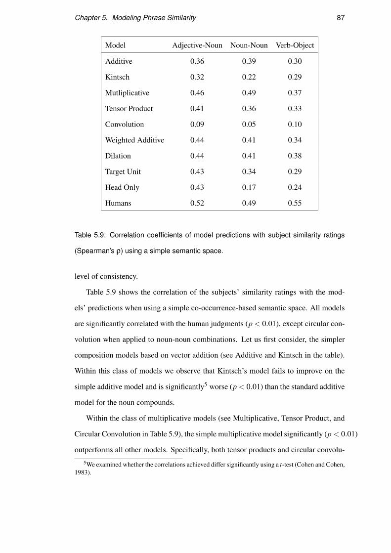
Chapter 5. Modeling Phrase Similarity 87
Model Adjective-Noun Noun-Noun Verb-Object
Additive 0.36 0.39 0.30
Kintsch 0.32 0.22 0.29
Mutliplicative 0.46 0.49 0.37
Tensor Product 0.41 0.36 0.33
Convolution 0.09 0.05 0.10
Weighted Additive 0.44 0.41 0.34
Dilation 0.44 0.41 0.38
Target Unit 0.43 0.34 0.29
Head Only 0.43 0.17 0.24
Humans 0.52 0.49 0.55
Table 5.9: Correlation coefficients of model predictions with subject similarity ratings
(Spearman’s ρ) using a simple semantic space.
level of consistency.
Table 5.9 shows the correlation of the subjects’ similarity ratings with the mod-
els’ predictions when using a simple co-occurrence-based semantic space. All models
are significantly correlated with the human judgments (p < 0.01), except circular con-
volution when applied to noun-noun combinations. Let us first consider, the simpler
composition models based on vector addition (see Additive and Kintsch in the table).
Within this class of models we observe that Kintsch’s model fails to improve on the
simple additive model and is significantly5 worse (p < 0.01) than the standard additive
model for the noun compounds.
Within the class of multiplicative models (see Multiplicative, Tensor Product, and
Circular Convolution in Table 5.9), the simple multiplicative model significantly (p < 0.01)
outperforms all other models. Specifically, both tensor products and circular convolu-
5We examined whether the correlations achieved differ significantly using a t-test (Cohen and Cohen,1983).

Chapter 5. Modeling Phrase Similarity 88
tion are significantly worse (p < 0.01). The multiplicative model is also significantly
better than the Additive one (p < 0.01). These results are observed across the board,
with adjective-noun, noun-noun, and verb-object combinations. It is worth noting that
circular convolution is the worst performing model. The tensor product itself, from
which circular convolution is derived, is significantly better (p < 0.01) in all experi-
ments. This indicates that the manner in which circular convolution projects the tensor
product down onto a lower dimensional space does not preserve the useful informa-
tion the product may have contained. In addition, the fact that the tensor product is
significantly worse than the simple multiplicative model indicates that the off diagonal
elements of the product, which are discarded in the simple multiplicative model, are
probably not contributing much to the composition.
We next consider the Weighted Additive and Dilation models. Recall that these
models are parametrized; in dilation models one word dilates the other by a factor λ
whereas the weighted additive model weights the constituents in the summation differ-
entially. As shown in Table 5.9 the two models perform similarly. This is not entirely
surprising, as both consist of a sum of the constituents multiplied by scalar factors
(see Equations 4.7 and 4.21). The performance of these models does not differ sig-
nificantly, except in the case of verb-object combinations where the dilation model
performs significantly better (p < 0.01). This model also fares similarly to the multi-
plicative model. The two models yield correlations that are not significantly different,
except in the case of noun-noun combinations, where the multiplicative model is better
(p < 0.01).
The two non-compositional models, Target Unit and Head Only, perform worse
than multiplicative composition, with this difference reaching significance (p < 0.01)
for noun-noun and verb-object combinations. In general, the target unit model per-
forms better than the head only model (it obtains significantly (p < 0.01) better cor-
relations for noun-noun combinations). This is not surprising, the target unit model
may be non-compositional, but nevertheless represents the semantics of the two words
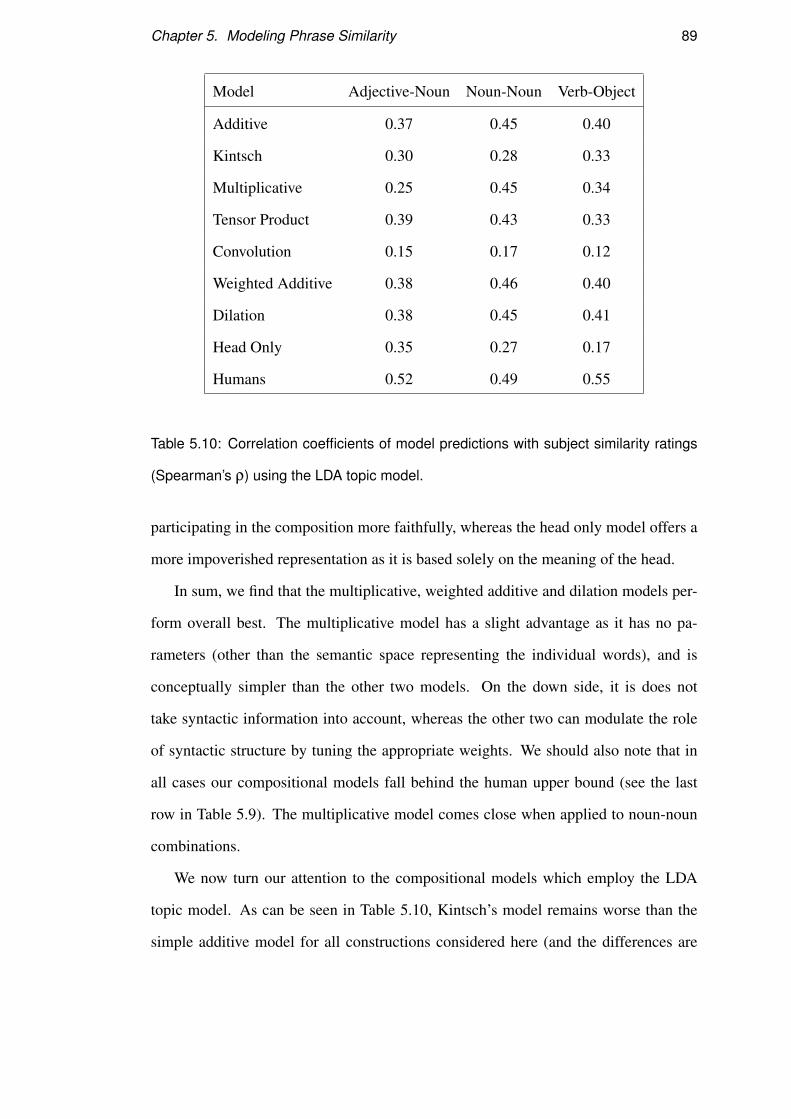
Chapter 5. Modeling Phrase Similarity 89
Model Adjective-Noun Noun-Noun Verb-Object
Additive 0.37 0.45 0.40
Kintsch 0.30 0.28 0.33
Multiplicative 0.25 0.45 0.34
Tensor Product 0.39 0.43 0.33
Convolution 0.15 0.17 0.12
Weighted Additive 0.38 0.46 0.40
Dilation 0.38 0.45 0.41
Head Only 0.35 0.27 0.17
Humans 0.52 0.49 0.55
Table 5.10: Correlation coefficients of model predictions with subject similarity ratings
(Spearman’s ρ) using the LDA topic model.
participating in the composition more faithfully, whereas the head only model offers a
more impoverished representation as it is based solely on the meaning of the head.
In sum, we find that the multiplicative, weighted additive and dilation models per-
form overall best. The multiplicative model has a slight advantage as it has no pa-
rameters (other than the semantic space representing the individual words), and is
conceptually simpler than the other two models. On the down side, it is does not
take syntactic information into account, whereas the other two can modulate the role
of syntactic structure by tuning the appropriate weights. We should also note that in
all cases our compositional models fall behind the human upper bound (see the last
row in Table 5.9). The multiplicative model comes close when applied to noun-noun
combinations.
We now turn our attention to the compositional models which employ the LDA
topic model. As can be seen in Table 5.10, Kintsch’s model remains worse than the
simple additive model for all constructions considered here (and the differences are

Chapter 5. Modeling Phrase Similarity 90
statistically significant (p < 0.01)). Regarding compositional models based on multi-
plication, we observe that tensor products and the simple multiplicative model yield
comparable performances for noun-noun and verb-object combinations. They differ
for adjective-nouns with the tensor product being significantly better (p < 0.01). Cir-
cular convolution remains the worst performing model. Not surprisingly, Weighted
Additive and Dilation models obtain almost identical performances. And they are not
significantly different from the simple Additive model. The non-compositional model
(Head Only) is significantly worse than these models. Comparing the spatial and topic-
based representations reveals that the multiplicative composition model on the simple
semantic space is significantly (p < 0.01) better than the dilation model with LDA,
except in the verb-object experiment, where there is no significant difference between
them.
5.3.5 Discussion
For the simple semantic space, no model significantly outperformed the simple mul-
tiplicative model. In contrast, for the LDA representations, no model significantly
outperformed the simple additive model. The weaker performance of the multiplica-
tive model on the LDA representations can be attributed to the fact that these vectors
are much sparser, and multiplication of their components tends to result in a loss of
useful information when a non-zero component is multiplied by zero. More difficult
to explain is the fact that no syntax based model outperforms either of these sim-
ple bag-of-words models. In Section 2.3 we discussed Pinker’s (1994) assertion that
composition is not blending. Yet, the simple additive and multiplicative models are
essentially forms of blending, producing composed vectors which are somewhat sim-
ilar to both the inputs. Syntactic models, which differentiate the contributions of the
two constituents, seem like they ought to provide a more effective model of seman-
tic composition. For example, our novel weighted additive and dilation models treat
their constituents differently and also allow different parameter values for each syn-

Chapter 5. Modeling Phrase Similarity 91
tactic structure. However, while they produced competitive results on all the phrase
types for both spaces, they did not significantly outperform the syntaxless rival. This
may be attributable to the fact that while they do allow a dependence on syntax, it is
not a particularly sophisticated dependence. In fact, both models are essentially the
weighted sum of the two constituents, and thus the composed vector is something like
both inputs, but a little more like one than the other. Such a simple treatment of syntax
appears to be insufficient to outperform the simpler non-syntactic models. Nonethe-
less, these models did outperform the other syntax based alternatives, in particular
circular convolution.
Circular convolution is designed to allow two vectors to be bound into a single
representation of the same dimension, in such a way that this composite vector can be
broken down into the original components again. As we discussed in Section 2.2, this
means that the representations it forms act like memories for complex structures, al-
lowing the recall of component parts after binding. However, we then argued in Section
2.3 that experiments on sentence recall (Sachs, 1967, 1988; Begg, 1971) demonstrate
that semantic composition is not simply equivalent to memory for constituents and
their stucture. Our experiments confirm this line of reasoning: the poor performance
of circular convolution indicates that vector binding is not by itself sufficient to model
the semantic processes of composition. While circular convolution may be an ade-
quate model of symbol concatenation, this syntactic operation is not the same thing as
semantic composition. In modeling the composition of a predicate and argument, it is
not enough to simply bind the representation of one to the representation of the other,
we must instead model the interaction between their meanings and their integration to
form a whole.
Interestingly, circumventing this issue, by treating the phrase as a single non-
compositional unit, yields results inferior to several of the compositional models. This
is somewhat surprising, as the target unit approach might be expected to produce a
representation more specific to the meanings of the words as they occur in the phrase.

Chapter 5. Modeling Phrase Similarity 92
In contrast, the semantic representations used in the compositional approach are gen-
eral to all instances of the constituent words. Nonetheless, the compositional models
produce representations that are more effective in predicting human similarity judge-
ments.
Currently, few of our models outperform the simple multiplicative model on this
task, even though it lacks a dependence on syntax. Of course, this simplicity has
advantages: it is fast and easy to compute, it does not need to be optimised for each
syntactic structure, and it can be applied in a bag-of-words manner, without regard
to syntactic structure. This latter trait will be exploited in the following chapter to
construct incremental representations for language modelling. Nonetheless, a model
of composition which can exploit syntax effectively is still desirable. However, while
our models lack the necessary syntactic sophistication the subjects ratings gathered in
this chapter will continue to provide a means of evaluation as distributional models of
composition develop.
5.4 Conclusions
In this chapter we demonstrated that distributional models of semantic composition
can be evaluated in terms of their ability to predict human similarity ratings for pairs
of phrases. We gathered such judgements for subject-verb, adjective-noun, noun-noun
and verb-object constructions, and used them to evaluate a number of composition
functions applied to two distinct forms of distributional representation: a simple se-
mantic space and an LDA topic based model. The correlation of the human ratings with
the model predictions reveals that, of the unparameterised models, the simple multi-
plicative model is the best performing model on the simple semantic space whereas
the simple additive model is best for LDA. We attribute the disparity in performance
to the sparsity of the LDA representations. The simple semantic space contains highly
distributed representations, with the semantic content spread across the great variety of

Chapter 5. Modeling Phrase Similarity 93
contexts a target word occurs in. In contrast, topic models tend to produce representa-
tions in which the vast majority of topics are inactive (i.e., zero) and when these topics
are multiplied by other topics, the result is zero. Thus, multiplicative combinations of
sparse representations tend to result in a loss of useful information. Among the param-
eterised models, the dilation model gives results close to the best performance across
both spaces.
The major limitation of these evaluations is that they are constrained to very simple
constructions. As argued in Section 5.1, this was a deliberate choice allowing us to iso-
late a single syntactic structure and eliminate other confounding factors. Nonetheless,
future work will need to evaluate the representations of more complex structures, in-
volving not only multiple syntactic relationships but also more complex constructions
such as relative clauses.
However, before tackling this phrase similarity task in more depth, we would like to
confirm that the results presented in this chapter are relevant outside the domain of the
experiments we have considered so far. In particular, finding a similar pattern of results
in other tasks would help to underscore the validity of this evaluation. Moreover, it
would be desirable to be able to automate the evaluation of compositional models
on a corpus, without requiring human ratings. A programme of human experiments
to cover the full richness and diversity of language would be impractical. Ideally, a
corpus based task would also demonstrate the practical utility of distributional models
of composition.
In the following chapter, we will adapt the models of phrase similarity used here to
produce a compositional language model. From the assumption that upcoming words
should be semantically coherent with their history, we will derive probabilities from
distributional representations of words and histories. In particular, the representation of
prior history will be constructed incrementally using a compositional model. We will
evaluate the effectiveness of these composition operations in terms of the perplexity of
the resulting language model on a test set.

Chapter 6
Language models based on Vector
Composition
Chapter 5 evaluated a number of vector composition functions against similarity rat-
ings for pairs of short phrases. While this approach does give a fairly direct insight into
semantic similarity and compositional representations, it can be criticised on a number
of fronts. Firstly, the amount of data that can be gathered in this way is limited by the
need to recruit participants and convince them to repetitively perform the task without
losing interest. Secondly, the materials on which the judgements are made are limited
and have been carefully selected, rather being representative of the range of construc-
tions found in natural text. Lastly, the elicited ratings are the product of an artificial
experimental task, the relation of which to natural linguistic behaviour is unclear.
Ideally, we would like to augment our evaluation with a task which is based on large
quantities of natural data. In addition we would like to demonstrate that the issue of
vector composition has practical consequences. For these reasons, the present chapter
investigates how vector composition models from the previous chapters can be applied
to language modelling. Language modelling is one of the fundamental components
of computational linguistics, being applied in speech recognition, machine translation
and many other tasks. For our purposes, it also provides a means of testing whether
94
Chapter 6. Language models based on Vector Composition 95
the semantic relationships hypothesised by our compositional models relate to what
is found in naturally occurring linguistic data. The basic idea, which has been imple-
mented in a variety of ways (Bellegarda, 2000; Coccaro and Jurafsky, 1998; Gildea
and Hofmann, 1999), is that each new word in a sentence should be semantically simi-
lar to the prior context. This simple approach to modelling the semantic dependencies
between the parts of a sentence allows us to enforce an overall semantic coherence on
its subject matter.
The contribution of the work presented here is that we examine the question of how
to construct a representation of prior context by composing the vectors representing
the words it contains. This requires an incremental approach to the construction of
semantic representations, and the simple additive and multiplicative functions are well
suited to this task. We show that these composition models can function as a language
model, with relatively minor modifications. We evaluate them for both the simple
semantic space and LDA vectors in terms of the perplexity of the derived language
model on a held out set.
As a stand alone language model, we find that this approach is only weakly pre-
dictive, as might be expected given that it has little to say about word order. We there-
fore use it to modulate the output from a trigram language model, and show that this
improves performance by incorporating dependencies to content words outside the tri-
gram window. We also show that interpolating with a syntactic language model results
in further improvements.
In Section 6.1, we give an overview of language modelling. We then examine
vector composition within this perspective in Section 6.2. Finally, Section 6.3 evaluates
the compositional language models and Section 6.4 summarises and draws conclusions
from this work.

Chapter 6. Language models based on Vector Composition 96
6.1 Language models
A language model is a means of assigning probabilities to texts, that is to sequences
of words. In the research presented here we focus on the probability of sentences, but
longer texts, e.g. paragraphs or whole documents, can also be modelled. Such prob-
ability distributions have many practical applications for example in guiding speech
recognition or machine translation, but they are also relevant to the investigation of the
cognitive processes that enable linguistic behaviours. Ultimately, a successful cogni-
tive model of the processes of language production ought to be able to tell us which
word sequences are likely to be found in natural text and which are not. Furthermore,
the probability of a text can also be used in modelling its comprehension, with high
probability sequences being read more quickly than those with low probability.
Thus, there are a number of practical and theoretical reasons for taking an interest
in modelling the probabilities of word sequences. At its most general this requires
deriving a joint probability model of the sequence. Commonly, however, the joint
probability is expressed as a product of conditional probabilities as in Equation 6.1.
p(w1,w2, . . .wn) = p(w1)p(w2|w1) . . . p(wn|wn−1 . . .w2,w1) (6.1)
Although this is provably true for all distributions, expressing the joint distribution in
this way is most useful when the dependencies being exploited by the language model
are indeed of this form, that is when a word is only dependent on previous words to its
left. Such a model will be incremental in the sense that it processes the input one word
at a time, conditioning the probability of the next word only on the previous history of
already processed words. This incrementality can be useful practically, in integrating
with the other components of a speech recognition system, and also cognitively consis-
tent with the incrementality of the human language processor (Tanenhaus et al., 1995;
Marslen-Wilson, 1973; Konieczny, 2000).
As already intimated, in assigning probabilities to sequences, language models ex-
ploit dependencies between the parts. So, for example either is typically followed at

Chapter 6. Language models based on Vector Composition 97
some point by or, and a language model, sensitive to such long range dependencies,
may use this fact to deflate the probabilities of sequences which break this rule. Al-
ternatively, a language model may be attuned to short range dependencies, such as
the fact that chief operating is almost always followed immediately by officer. It is
clear that the dependencies within any sentence of a reasonable length will be both nu-
merous and complex, posing difficulties for any system that attempts to handle all of
them. The ideal language model would of course exploit all the structure of language
to make the most accurate predictions of the probability of a text, but in practice the
need to estimate the model’s parameters from a corpus makes this impractical for cur-
rent approaches. Instead, effective language models exploit a limited set of the most
important dependencies. In the following discussion we outline the various types of
dependencies and how they may be modelled.
6.1.1 Syntactic Models
The obvious way to characterise linguistic structure would be in terms of syntax, and
syntactic language models express the probability of sentences in terms of these de-
pendencies. For example a Probabilistic Context Free Grammar (PCFG) associates a
probability with each rule in a CFG (Booth, 1969). The joint probability of a parse
tree, T , is then the product of the rules, r, that expand each node, n, and the probability
of a sentence, S, is a sum over the set of its parse trees, τ(S).
p(S) = ∑T∈τ(S)
p(T ) = ∑T∈τ(S)
∏n∈T
p(r(n)) (6.2)
However, the probabilities produced by a PCFG are not very predictive. While this
approach captures dependencies at the level of syntactic types, e.g. nouns are modified
by adjectives, it tends to ignore lexical dependencies, e.g the adjective happy rarely
modifies the noun sky.
To remedy this shortcoming, the grammar can be lexicalised. That is, non-terminals
are annotated with some information about the lexical items into which they expand.

Chapter 6. Language models based on Vector Composition 98
For example, Charniak (2001) implements a language model based on immediate head
parsing. In this case the expansion of a constituent is conditioned on its lexical head,
and this allows the relation between the head and its dependents to be modelled. It does
not, however, model relations between dependents of the same head, treating them in-
stead as independent. Of course, additional lexical conditioning information can be
introduced into the grammar, but dividing the grammatical categories more and more
finely will eventually lead to problems with the sparsity of data.
It is also worth noting that conditioning the probability of words on their heads is
not generally consistent with incrementality. When a dependent can precede its head,
e.g., adjectives precede their head noun, the head will not be available for conditioning
the probability of the dependent if the sentence is processed incrementally in a left
to right fashion. Roark (2001) develops an incremental syntactic language model by
employing a couple of variations. First, a left corner transform is applied to the gram-
mar, which allows complete rooted trees to be built on the left context by removing
the problem of non-terminating left recursion. This allows the identification of all the
dependencies in this prior history which could be used to condition the probabilities of
upcoming words. Second, a general approach to selecting this conditioning informa-
tion based on a tree walking algorithm is employed. In practice, the best performing
model selects lexical heads where available, and nearby lexical items otherwise, but
alternative models also consider non-lexical information, such as POS tags.
Both these language models are supervised, in that they require a treebank of parsed
text on which to be trained. Parsing and annotating a corpus by hand is time consum-
ing, and consequently the quantity of such data is much more limited than simple raw
text. In practice, syntactic language models are often interpolated with n-gram models,
which are trained on raw text, to ameliorate this problem. Unsupervised approaches
can infer syntactic structures from raw text, but are slower and less accurate. In addi-
tion, however a probabilistic grammar is trained, applying it as a language model will
be based on a search over the space of parse trees, which is typically resource inten-

Chapter 6. Language models based on Vector Composition 99
sive. Thus, although syntax gives us the most complete formalism for describing the
structure of sentences, in practice the fact that this structure is not directly observable
in raw text inhibits its utility.
6.1.2 Ngram Models
An alternative to exploiting syntactic structure for language modelling is simply to use
linear order. The linear order of words in a sentence is explicit and relatively sim-
ple, in contrast to syntax, which has a hierarchical structure and can only be inferred
implicitly. In terms of linear order, the strongest dependencies are highly local, be-
tween words that are very close to each other. Thus, effective language models can
be built by simply conditioning the probabilities on the most recent prior words. In
other words, we truncate the history when we consider the conditional probability of
a word. These n-gram models approximate the full conditional probability of a word
by its conditional probability given only the last n−1 words, for some low value of n,
e.g., n = 3.
p(wn|wn−1, . . .w2,w1)≈ p(wn|wn−1,wn−2) (6.3)
Ignoring dependencies to words outside this n word window reduces the complexity
of the model to a manageable scale and the probabilities can be derived from counting
n-grams in a corpus. The simplest approach would be to convert counts directly to
probabilities using the maximum likelihood estimate as in Equation 6.4.
p(w3|w2,w1) =f req(w3,w2,w1)
f req(w2,w1)(6.4)
Unfortunately, this approach assigns all the probability mass only to n-grams which
were seen in the training data. However large the training corpus it is unlikely that it
will contain every plausible n-gram. This means that in applying the model to novel
data there will be word sequences which are assigned zero probability. Worse, there
will even be some sequences which cannot be assigned a meaningful probability be-
cause the denominator in Equation 6.4 is zero. The solution is to use a smoothing
Chapter 6. Language models based on Vector Composition 100
technique to shift some of the probability mass onto unseen events. Two questions
need to be addressed: how much probability mass to reassign and how to distribute it
among the unseen events.
There are a number of approaches to answering both these questions. For exam-
ple, absolute discounting (Ney et al., 1994) provides a very simple means of deciding
how much probability mass to re-assign, by simply subtracting the same amount from
all non-zero counts. These quantities can then be redistributed to the unseen events.
Whereas this approach discounts all counts by the same amount, the Good-Turing
(Good, 1953) method takes into account the number of different n-grams having a
given count in determining the discounts. However discounting is carried out, this still
leaves open the question of how to assign it across the zero counts. A common method
for distributing the discounted probability mass over unseen events is in terms of back
off probabilities (Katz, 1987). The basic idea is to use a lower order model, i.e. with
coarser dependencies, to assign probabilities to the zero count events. So, a trigram
model could back-off to a bigram model, with the bigram counts being less affected
by sparsity, and the bigram model might itself back off to a unigram model. Typically,
these lower order models are estimated in the same way as the top level model, in terms
of counting n-grams. Kneser and Ney (1995) show that this may not be optimal and
propose a form of back off in which the lower order models are specifically adapted to
the task of making predictions for unseen events.
Another issue that arises in applying a trained model to a novel corpus is that of
domain differences. It is obvious that the vocabulary of documents from a news corpus
will differ significantly from those in a biomedical corpus, and a model trained on
one will not be optimal when tested on the other. Moreover, even within the same
general domain, data from different sources can have significantly different statistics.
For example, Rosenfeld (1996) found that a trigram model trained on the Wall Street
Journal doubled its perplexity when applied to Associated Press articles.
A variety of approaches to domain adaptation for n-gram models have been pro-

Chapter 6. Language models based on Vector Composition 101
posed (e.g., see Bellegarda, 2004). For example, Kuhn and de Mori (1990) proposed
interpolating the unadapted model with a model derived from a cache of recently ob-
served words from the test corpus. In this way the probabilities of common vocabulary
items from the test domain are increased. While this only incorporates a dependency
between a word and its own re-occurence later in the corpus, Rosenfeld (1996) used
a maximum entropy framework to select arbitrary trigger word pairs. In this way en-
countering a given trigger can modulate the probabilities of a number of related words
in its wake.
Rather than thinking of these models as adapting a language model to a new do-
main, we can instead think of them as extending the model to include history outside
the n-gram window. Both the cache and the triggers allow longer range dependencies
between words to be captured. Nonetheless, these models are still based on dependen-
cies between specific individual words, albeit over greater spans.
6.1.3 Semantic Models
Both the syntactic and n-gram models exploit lexical dependencies to make predic-
tions. But there are of course more general factors which might help in predicting
which words are likely to come next. In particular, any given text will have some over-
all subject matter, and its particular content will generally be coherent and relevant
to that subject. A common approach to capturing these sort of effects in a language
model is to base the probability of an upcoming word on its similarity to the history
of previous words (Bellegarda, 2000; Coccaro and Jurafsky, 1998; Wandmacher and
Antoine, 2007; Gildea and Hofmann, 1999). In this way, the language model prefers
words which fit the semantic topic established so far. Two issues need to be resolved
in implementing this idea. First, a probabilistic measure for comparing the semantic
representations of a word and its history is required. Second, building a representation
of the history requires some means of combining word representations.
With representations derived from Latent Semantic Analysis (Landuaer and Du-

Chapter 6. Language models based on Vector Composition 102
mais, 1997) the obvious way to compare vectors is in terms of the cosine measure,
and this is the approach taken by Bellegarda (2000) and Coccaro and Jurafsky (1998).
Unfortunately, the cosine measure does not directly yield a valid probability because
its values do not sum to one. Worse, it even produces negative values for some com-
parisons. The solution proposed by Coccaro and Jurafsky (1998) is to rescale and
normalise these values to produce a valid probability measure. They first add or sub-
tract the same amount to all values, shifting the minimum to zero, and then normalise,
producing a distribution that sums to one. Following that, to increase the dynamic
range, the values are raised to some power (e.g. 7) and renormalised.
While this method defines the transformation of cosine values into probability es-
timates algebraically, Bellegarda (2000) takes a different approach by defining this
function empirically. Specifically, the probability associated with a given cosine value
is based on the number of times a value of that size was encountered in the training
data.
Whatever transformation is used, the cosine measure is still nonetheless an imper-
fect basis from which to derive probabilities. In particular, it is simply a measure of
similarity and takes no account of the underlying frequency of the items involved. So,
for example, otiose and lazy may be equally similar to some context, but the latter,
being more common, may nonetheless be more probable. The approach of Gildea and
Hofmann (1999) overcomes this difficulty by using representations constructed with
pLSA, which have a direct probabilistic interpretation. The pLSA model is based on
the assumption that each document in a collection is a mixture of topics, which are
themselves unigram distributions over the vocabulary. The probability of finding a
word, w, in a document, d, is then expressed as a sum over topics, t.
p(w|d) = ∑t
p(w|t)p(t|d) (6.5)
If the history can be treated as a kind of document then this expression provides a
means of deriving probabilities naturally and directly, avoiding the need for ad-hoc
transformations.

Chapter 6. Language models based on Vector Composition 103
This still leaves the question of how to construct the representation of history. This
will involve combining the individual word vectors in some way to form a single rep-
resentation of the whole prior context. Coccaro and Jurafsky (1998) do this by simply
summing them, which is motivated in terms of the geometric interpretation of vectors.
Bellegarda (2000) instead appeals to the mathematical foundations of the LSA proce-
dure to represent the history as a pseudo-document, which is basically a weighted sum
of the same word vectors. Similarly, Gildea and Hofmann (1999) derive their approach
from the representation of documents within pLSA. They use a single iteration of an
online EM algorithm to infer a pseudo-document representation for the history.
While these methods of constructing history representations are reasonably well
motivated in terms of the assumptions of the models to which they are applied, with-
out an empirical investigation of the performance of a range of approaches we cannot
determine how optimal they are. In particular, Chapter 4 discussed a number of com-
position functions which could be applied to the combination of the word vectors in
the prior history.
The elements of the language model that have been defined so far (the construction
of the history vector and its comparison to upcoming words) are only weakly predic-
tive. The model, as it stands, only gives an indication of which words are coherent with
the subject matter so far, and takes no account of the structure or order these words are
likely to be found in. Typically, the scheme is extended by integrating the semantic
language model with an n-gram model. Bellegarda (2000) and Gildea and Hofmann
(1999) both use a rescaling approach to combine the probabilities of the two models:
p(w|h1,h2) ∝ p(w|h1)p(w|h2)
p(w)(6.6)
where h1 is the n-gram representation of history and h2 is the semantic representation
of history. In other words, the n-gram model is rescaled by a factor based on the ratio of
the semantic probability to the unigram probability. This can be shown to be equivalent
to an assumption that h1 and h2 are independent. Coccaro and Jurafsky (1998) instead
base their integration on the geometric mean of the two models. They also incorporate

Chapter 6. Language models based on Vector Composition 104
a confidence factor for determining the strength of the semantic models contribution.
Extensions on the basic semantic language models sketched above involve repre-
senting the history by multiple LSA models of varying granularity in an attempt to cap-
ture topic, subtopic, and local information (Zhang and Rudnicky, 2002); incorporating
syntactic information by building the semantic space over words and their syntactic
annotations (Kanejiya et al., 2004); and treating the LSA similarity as a feature in a
maximum entropy language model (Deng and Khundanpur, 2003).
Instead of constructing separate semantic and n-gram models which then need to be
combined in some way, Wallach (2006) integrates a topic model with a bigram model
directly. Whereas a standard LDA topic model expresses the content of a document as
a mixture of topics, with each topic being a unigram distribution over the vocabulary,
Wallach (2006) expresses the content of a document as a mixture of bigrams. In this
formulation, as in LDA, each document is associated with a distribution over topics,
but the topics in this case are bigram distributions, and in this way the model captures
both the local bigram structure and the topical semantic structure in one model.
6.1.4 Connectionist Language Models
The language models discussed so far in this section have exploited a set of depen-
dencies which were fixed in advance: e.g., to the head of a phrase or to the most re-
cent previous words. Connectionist approaches to modelling the structure of language
have taken a different approach by implementing distributed representations that learn
which features and dependencies are most useful.
Rather than being concerned with optimising a probabilistic model of word se-
quences for application to some practical task, early connectionist work on language
was often motivated by theoretical criticisms from the symbolic camp (Fodor and
Pylyshyn, 1988). This led to a focus on the question of how linguistic structures could
be represented in distributed representations and whether these representations could
be learned. For example, Elman (1991) applied a simple recurrent network to the

Chapter 6. Language models based on Vector Composition 105
problem of predicting the next word in sentences generated by a toy grammar. Exami-
nation of the network’s hidden units showed that the representation learned to encode
both lexical and grammatical information.
In contrast, the concern of Bengio et al. (2003) is directed to the practical benefits of
connectionist models, rather than their theoretical representational capacities. In this
case distributed representations are employed to reduce the free parameters in an n-
gram model and attain better generalisation. Each word in the vocabulary is associated
with a vector, and n− 1 of these vectors form the input to the network, representing
the n-gram context. These vectors and the function which predicts the next word from
them are learnt during training by stochastic gradient ascent on the log-likelihood of
the training data. The network itself has a feed forward architecture, with a single layer
of hidden units that combines the input word vectors to form a merged representation
which is used to predict probabilities for the next word. This combination of word
vectors has something in common with our vector composition models, being a way of
integrating word vectors to produce a single representation of a multi-word structure.
One major difference, however, is that the word vectors in this case are not designed
to represent the semantic properties of the words.
Mnih and Hinton (2007) propose a log-bilinear model in which, again, each word
in the vocabulary is associated with a distributed representation. However, in this case
the prediction of upcoming words is not simply made in terms of a function computed
by a feed forward network. Instead, the probability of the next word is based on its
similarity, as measured by the dot product, of its word vector to a history vector derived
by combining the n− 1 prior input vectors. These word vectors and the combination
function are learnt by the network by maximising the log-likelihood of a training cor-
pus. Here too, although the representations cannot be considered a purely semantic,
the issue of vector combination we are considering is relevant.
Both connectionist models build vectors representing individual words and com-
bine them in some way to represent word sequences. The question of how best to

Chapter 6. Language models based on Vector Composition 106
implement this, specifically for semantic representations, is the general topic of this
thesis. Interestingly, both connectionist models make use of general additive func-
tions (Equation 4.2) in their approach to vector combination, without exploring what
multiplicative functions (Equation 4.3) could achieve.
6.2 Vector Composition
In this section we will develop a language model based on vector composition. As in
previous work, the conditional probability of a word given its history will be based on
the semantic similarity of that word to the history. In our case, however, we will inves-
tigate the influence of vector composition functions in constructing the representation
of the history. Where possible, we will make the implementation of the compositional
model as close to that presented in Chapter 5 as possible. So, we will use the same
definition of vector components and use the same simple additive and multiplicative
composition functions. However, lemmatisation will not be appropriate for the current
task. Another difference will be in the manner we measure similarity. While cosine
similarity was effective in modelling similarity ratings, we will argue that it has a num-
ber of drawbacks for this application. Nonetheless, our derivation of the new measure
will be a modification of cosine similarity.
Our focus will be on the simplest composition functions: the simple multiplicative
and additive functions. An obvious benefit of these functions is that they can be applied
in linear order, because they are insensitive to syntax and word order, making them
suitable for forming representations of sentence prefixes in a left to right, word by
word manner. Applying the syntactic composition functions would require not only
setting the parameters for all the syntactic structures in the grammar, but also figuring
out how to build representations for the partial trees of sentence prefixes, as opposed
to the complete phrases considered in Chapter 5.
In any case, the simple models proved to give robust results in modelling phrase

Chapter 6. Language models based on Vector Composition 107
similarity judgements. So far we have considered these functions in terms of their se-
mantic and vectorial properties. From the perspective of a language model, however,
it becomes important to understand their probabilistic properties. First we show how
these two composition functions can be given a probabilistic interpretation, and fol-
lowing that we derive a language model which compositionally constructs a semantic
representation of prior context. Experiment 3 then evaluates these language models in
terms of their perplexity on a news corpus.
6.2.1 Vector Composition from a Probabilistic Perspective
Experiments 1 and 2 examined the ability of vector composition models to simulate
human similarity ratings for phrases. We now want to motivate vector composition
as a basis for a probabilistic model by giving the simple additive and multiplicative
models a probabilistic interpretation.
The vector components we have been using, in the case of both the simple semantic
space and the LDA based representation, have the form of a ratio of probabilities:
vi =p(ci|w)p(ci)
(6.7)
where v is a vector representing the word w, and ci represents a context word in the
case of the simple semantic space, and in the case of LDA a topic. This component
definition was adopted because it performed well in modelling similarity ratings. How-
ever, we can also examine the probabilistic properties of these components in relation
to the composition functions we are considering.
Let us assume vectors u and v represent target words w1 and w2. Now, when we
compose these vectors using the multiplicative model and the components definition
in (6.7), we obtain:
hi = vi ·ui =p(ci|w1)
p(ci)p(ci|w2)
p(ci)(6.8)
Applying Bayes’ theorem:
hi =p(w1|ci)p(w2|ci)
p(w1)p(w2)(6.9)

Chapter 6. Language models based on Vector Composition 108
Assuming w1 and w2 are independent and applying Bayes’ theorem again, hi becomes:
hi ≈p(w1w2|ci)p(w1w2)
=p(ci|w1w2)
p(ci)(6.10)
By comparing to (6.7), we can see that the expression on the right hand side gives
us something akin to the vector components we would expect when our target is the
co-occurrence of w1 and w2. Thus, for the multiplicative model, the combined vec-
tor hi can be thought of as an approximation to a vector representing the distributional
properties of the phrase w1w2.
If multiplication results in a vector which is something like the representation of w1
and w2, then addition produces a vector which is more like the representation of w1
or w2. Suppose we were unsure whether a word token x was an instance of w1 or of w2.
It would be reasonable to express the probabilities of context words around this token
in terms of the probabilities for w1 and w2, assuming complete uncertainty between
them:
p(ci|x) =12
p(ci|w1)+12
p(ci|w2) (6.11)
Therefore, we could represent x with a vector, based on these probabilities, having the
components:
xi =12
p(ci|w1)p(ci)
+12
p(ci|w2)p(ci)
(6.12)
Which is exactly the vector averaging approach to semantic composition.
Thus, these two composition models have distinct probabilistic interpretations. The
multiplicative model is associated with the conjunction of its constituents, that is it
treats the pair as a phrase. Whereas, the additive model is based on disjunction, treating
the constituents as separate. The success of multiplication or addition as a model
of composition is likely then to depend on the appropriateness of conjunction and
disjunction in the underlying scheme in which vectors are constructed.

Chapter 6. Language models based on Vector Composition 109
6.2.2 Deriving a Language Model
Our aim now is to derive probabilities, p(w|h), given the semantic representations of
a word, w, and its history, h, based on the assumption that probable words should be
semantically coherent with the history. Semantic coherence may be measured in terms
of similarity, which is commonly calculated via the cosine of the angle between two
vectors:
sim(w,h) =w ·h|w||h|
(6.13)
w ·h = ∑i
wihi (6.14)
where w · h is the dot product of w and h. Coccaro and Jurafsky (1998) utilize this
measure in their approach to language modeling. Unfortunately, they find it necessary
to resort to a number of ad-hoc mechanisms to turn the cosine similarities into use-
ful probabilities. The primary problem with the cosine measure is that its values do
not sum to 1, as probabilities must. Thus, normalization over the entire vocabulary is
required. A further problem concerns the fact that such a measure takes no account
of the underlying frequency of w, which is crucial for a probabilistic model. For ex-
ample, encephalon and brain are roughly synonymous, and may be equally similar to
some context, but brain may nonetheless be much more likely, as it is generally more
common.
A better measure would take account of the underlying probabilities of the ele-
ments involved and produce values that sum to 1. Our approach is to modify the dot
product (Equation 6.14) on which the cosine measure is based. Assuming that our
vector components are given by Equation 6.7, the dot product becomes:
w ·h = ∑i
p(ci|w)p(ci)
p(ci|h)p(ci)
(6.15)
which we modify to derive probabilities as follows:
p(w|h) = p(w)∑i
p(ci|w)p(ci)
p(ci|h)p(ci)
p(ci) (6.16)

Chapter 6. Language models based on Vector Composition 110
This expression now weights the sum with the independent probabilities of the context
words and the word to be predicted. That this is indeed a valid probability can be seen
by the fact it is equivalent to ∑i p(w|ci)p(ci|h). However, in constructing a represen-
tation of the history h, it is more convenient to work with Equation 6.16 as it is based
on vector components (Equation 6.7) and can be readily used with the composition
models we are considering.
Equation 6.16 allows us to derive probabilities from vectors representing a word
and its prior history. We must also construct a representation of the history up to the nth
word of a sentence. To do this, we combine, via some (additive or multiplicative)
function f , the vector representing that word with the vector representing the history
up to n−1 words:
hn = f (wn,hn−1) (6.17)
h1 = w1 (6.18)
One issue that must be resolved in implementing Equation 6.17 is that the history
vector should remain correctly normalized. In other words, the products hi · p(ci) must
themselves be a valid distribution over ci. So, after each vector composition the history
vector is normalized over the vector components as follows:
hi =hi
∑j
h j · p(ci)(6.19)
Equations 6.16– 6.19 define a language model that incorporates vector composition.
To generate probability estimates, it requires a set of word vectors whose components
are based on the ratio of probabilities described by Equation 6.7.
6.2.3 Integrating with Other Language Models
The model defined above is based on little more than semantic coherence. As such
it will be only weakly predictive, since word order is largely ignored, which n-gram
models exploit. The simplest means to integrate semantic information with a standard

Chapter 6. Language models based on Vector Composition 111
language model involves combining two probability estimates as a weighted sum:
p(w|h) = λ1 p1(w|h)+(1−λ)p2(w|h) (6.20)
Linear interpolation is guaranteed to produce valid probabilities, and has been used, for
example, to integrate syntactic language models with n-gram models (Roark, 2001).
However, it will work best when the models being combined are comparably pre-
dictive and have complementary strengths and weaknesses. If one model is much
weaker than the other, linear interpolation will typically produce a model of interme-
diate strength (i.e., worse than the better model), with the weaker model contributing a
form of smoothing at best.
Instead, we use a rescaling approach (Kneser et al., 1997; Gildea and Hofmann,
1999). Based on Equation 6.16, we can express our semantic probabilities as the prod-
uct of the unigram probability, p(w), and a semantic component, ∆, which determines
the factor by which this probability should be scaled up or down given the context in
which it occurs.
p(w|h) = p(w) ·∆(w,h) (6.21)
∆(w,h) = ∑i
p(ci|w)p(ci)
p(ci|h)p(ci)
p(ci) (6.22)
Thus, it seems reasonable to integrate the n-gram model by replacing the unigram
probabilities with the n-gram versions.
p(wn) = p(wn|wn−1n−2) ·∆(wn,h) (6.23)
This is equivalent to assuming that h is conditionally independent of wn−1n−2.
This rescaling is only applied to content words, as the semantic representations
contain little useful information for function words. To obtain a true probability esti-
mate, p(wn) needs to be normalised, but the rescaling has to be carried out only on
content words, with function words retaining the straight n-gram prediction:
p(wn|wn−1n−2,h) = p(wn)
∑wc p(wc|wn−1n−2)
∑wc p(wc)(6.24)

Chapter 6. Language models based on Vector Composition 112
where the sum over wc is a sum over content words only. In other words, p(wn) is
normalised so that the total probability mass for content words is equal to the proba-
bility mass assigned to content words by the n-gram model. This leaves the remaining
probability mass assigned to function words unchanged.
In integrating our semantic model with an n-gram model, we allow the latter to
handle short range dependencies and have the former handle the longer dependencies
outside the n-gram window. For this reason, the history h used by the semantic model
in the prediction of wn only includes words up to wn−3 (i.e., only words outside the
n-gram).
We also integrate our models with a syntactic language model (Roark, 2001), as
this allows us to compare the benefits derived from incorporating long-range syntactic
dependencies to those derived from our semantic model. However, in this case we use
linear interpolation (Equation 6.20) because the models are roughly equally predictive
and also because linear interpolation is widely used when probabilistic parsers are
combined with n-grams and other information sources. This approach also has the
benefit of allowing the models to be combined without out the need to renormalize the
probabilities. In the case of the parser, normalizing across the whole vocabulary would
be prohibitive.
6.3 Experiment 3
6.3.1 Method
We experimented with additive and multiplicative composition functions, and two se-
mantic representations (LDA and the simpler semantic space model), resulting in four
compositional models. In addition to implementing the stand alone semantic com-
positional model, we integrated this model with a standard n-gram model (see Equa-
tion 6.23). We also compared our models against a state of the art syntactic language
model in order to assess the extent to which the information provided by the seman-

Chapter 6. Language models based on Vector Composition 113
tic representation is complementary to syntactic structure. Our experiments used the
grammar-based language model of Roark (2001), which is suitable for integration with
the semantic and n-gram components because of its incrementality.
All our models were evaluated by computing perplexity1 on a test set. Roughly, this
quantifies the degree of unpredictability in a probability distribution, such that a fair
k-sided dice would have a perplexity of k. More precisely, perplexity is the reciprocal
of the geometric average of the word probabilities and a lower score indicates better
predictions. We calculated this measure by taking negative logs of the probabilities,
averaging them, and then exponentiating that value:
perplexity = ∏ p−1/N = x∑− logx(p)/N (6.25)
Although this is a commonly used metric for evaluating language models there is no
established method of testing the significance of differences in this measure. Here, we
chose to not only report a single overall perplexity for the whole test set but to also
perform significance tests at the level of individual words, where we could identify a
range of variation within the results for each model and compare that to the variation
between models. It would be possible to calculate per-word perplexities but these val-
ues have an extremely skew distribution, and it is difficult to decide what should be
tested and how that test relates to the overall perplexity values. Instead, we performed
a paired t-test on the value −log(p), which is the log of the per-word perplexity, and
these values have a distribution much closer to normality. The t-test tests for a differ-
ence in means and the mean of −log(p) is just the log of the overall perplexity, giving
a fairly direct relationship between the hypothesis test and the perplexity values.
1Word error rate is an alternative measure for evaluating language models. Essentially this quantifiesthe benefit the model brings to a speech recognition system. Since this requires integration with anacoustic model, and we are not directly interested in speech recognition anyway, we choose to useperplexity as our evaluation metric.

Chapter 6. Language models based on Vector Composition 114
6.3.2 Data
The experiments were based on data from the Wall Street Journal in the BLLIP cor-
pus (years 1987–89) and Penn Treebank (1989). We pre-processed and partitioned
the BLLIP corpus into training, test and development sets as described in Chapter
3. Specifically, numbers were replaced with the symbol 〈num〉, and a vocabulary
of 20,000 words was chosen and the remaining tokens were replaced with 〈unk〉. From
this data, a 38,521,346 word training set was used to construct the trigram language
model and the semantic representations, while perplexity results were calculated on a
50,006 word test set2. The Penn Treebank was pre-processed in the same way, with
the whole treebank being used as a training set for the syntactic language model.
6.3.3 Model Parameters
The semantic components of the language models were based on the simple seman-
tic space and LDA model constructed on the BLLIP corpus described in Chapter 3.
Our composition models were the unparametrised simple additive and multiplicative
functions.
We integrated our compositional models with a trigram model which we also trained
on BLLIP. The model was built using the SRILM toolkit (Stolcke, 2002) with backoff
and modified Kneser-Ney smoothing (Chen and Goodman, 1999). Following previous
work on syntactic language modeling (Roark, 2001; Charniak, 2001; Chelba and Je-
linek, 1998), we trained the parser on sections 2–21 of the Penn Treebank containing
936,017 words. Note that Roark’s (2001) parser produces prefix probabilities for each
word of a sentence which we converted to conditional probabilities by dividing each
current probability by the previous one.

Chapter 6. Language models based on Vector Composition 115
Model Perplexity
Unigram 2604
AddSSM 2099
MultiplySSM 1734
AddLDA 1593
MultiplyLDA 6659
Table 6.1: Perplexities for unigram, and compositional language models on content
words in the test set; subscripts SSM and LSA refer to the semantic space and LDA
models, respectively.
6.3.4 Results
Table 6.1 shows perplexity results for the stand alone semantic models. Because these
models are based purely on semantic similarity they are applied only to the 26,583
content words in the test set, and not function words such as the and with. With regard
to the simple semantic space model (SSM), we observe that both additive and multi-
plicative approaches to constructing history are successful in reducing perplexity over
the unigram baseline, with the multiplicative model outperforming the additive one.
A t-test confirms that these differences are significant (p < 0.01). Since the unigram
model takes no history into account, this demonstrates that these models successfully
capture at least some of the semantic dependencies within the test sentences.
The results for the LDA model are also reported in the table. This model reduces
perplexity with an additive composition function, but performs worse than the unigram
with a multiplicative function. Again, these differences are significant (p < 0.01). The
additive LDA model also significantly (p < 0.01) outperforms the simple semantic
space models and is the best performing model overall.
Table 6.2 reports the perplexities for these semantic models when they are inte-
2The test set was drawn from the year 1987 to avoid overlap with the Penn Treebank.

Chapter 6. Language models based on Vector Composition 116
Model Perplexity
n-gram 77.42
n-gram+AddSSM 75.24
n-gram + MultiplySSM 73.77
n-gram+AddLDA 73.06
n-gram+MultiplyLDA 143.66
parser 173.35
n-gram + parser 75.23
n-gram + parser + AddSSM 73.27
n-gram + parser + MultiplySSM 71.27
n-gram + parser + AddLDA 70.02
n-gram + parser + MultiplyLDA 91.08
Table 6.2: Perplexities for n-gram, composition and syntactic language models, and
their combinations on the full test set; subscripts SSM and LSA refer to the semantic
space and LDA models, respectively.
grated with an n-gram model. In this case, the perplexities are for the whole vocabu-
lary, with the n-gram probabilities for function words left unaltered but content words
rescaled by the semantic model. Here, the results follow much the same pattern as be-
fore with the multiplicative model producing significantly (p < 0.01) better results for
the simple semantic space and the additive LDA model being significantly (p < 0.01)
better than all the other models including the simple semantic space models. Com-
parison to the plain n-gram baseline shows that the semantic models are successful in
exploiting semantic dependencies to words outside the n-gram window, except notably
for the multiplicative LDA model.
For comparison, Figure 6.1 plots the perplexity of the combined LDA and n-gram
models against the number of topics. Increasing the number of topics produces higher

Chapter 6. Language models based on Vector Composition 117
Figure 6.1: Perplexity versus Number of Topics for the LDA models using additive and
multiplicative composition functions.
dimensional representations which ought to be richer, more detailed and therefore more
predictive. While this is true for the additive model, a greater number of topics actu-
ally increases the perplexity of the multiplicative model, indicating it has become less
predictive.
We compared these perplexity reductions against those obtained with a syntactic
language model. Following Roark (2001), we combined the probabilistic parser with
a trigram model using linear interpolation (the weights were optimized on the devel-
opment set). This model (n-gram + parser) is significantly (p < 0.01) outperformed
by our best compositional models (n-gram + MultiplySSM, n-gram + AddLDA). While
both models incorporate long range dependencies, the parser is trained on a hand anno-
tated treebank, whereas the compositional model uses raw text, albeit from a larger cor-

Chapter 6. Language models based on Vector Composition 118
pus. Furthermore, three interpolated compositional models (n-gram + parser + AddSSM,
n-gram + parser + MultiplySSM and n-gram + parser + AddLDA) are all also significantly
better then the interpolated model without composition (n-gram + parser) This sug-
gests that these semantic models are encoding useful predictive information about
long range dependencies, which is distinct from and potentially complementary to
the parser’s syntactic information about such dependencies. The interpolated additive
LDA model (n-gram + parser + AddLDA) significantly (p < 0.01) outperforms all the
other models.
6.3.5 Discussion
Our results indicate that the compositional models are successful in representing se-
mantic dependencies both on their own and in combination with an n-gram model.
Moreover, by integrating with a parser we achieved further perplexity reductions,
demonstrating that these syntactic and semantic components exploit distinct long range
dependencies.
For the simple semantic space, both the additive and multiplicative models pro-
duced predictive representations. Interestingly, in the LDA setting only the additive
model produced improvements over the baseline with the multiplicative model prov-
ing detrimental. Increasing the representational power of the LDA model, by using a
greater number of topics, rendered the multiplicative model less predictive.
Given this lack of performance, we would like to know why the multiplicative
model is not effective when applied to the LDA representation. In particular, Equations
6.8 to 6.10 of Section 6.2.1 appear to show that the multiplicative model can be derived
from some simple assumptions. However, our experimental results demonstrate that
this derivation is not valid for LDA.
The problem arises because in the LDA model each word of a phrase may be gen-
erated by a distinct topic. The representation of the whole phrase, therefore, should
contain all these topics. However, the derivation of the multiplicative model assumes

Chapter 6. Language models based on Vector Composition 119
that the topics which are relevant to the whole phrase are those that could generate all
its constituents. Addition by contrast was related in Section 6.2.1 to a disjunction of
the words in a phrase, and in this way is more effective at gathering the disjoint topics
associated with the words in a phrase into a single representation.
The multiplicative model is much more successful on the simple semantic space.
We can explain this in terms of the fact that if a context word is associated with a whole
phrase, it is likely to be associated with each of the constituents. In other words if c
never appears in the context around w, it is unlikely to appear in the context surround-
ing any phrase containing w.
More pragmatically, the effectiveness of these compositional models is related to
the sparsity of the underlying vector representations. LDA representations tend to be
fairly sparse, and multiplication increases this sparsity resulting in useful information
being discarded. Whereas, the simple semantic space representations are much more
distributed and multiplication in this case is effective in whittling down these vectors
to the most relevant components.
6.4 Conclusions
In this chapter we demonstrated that a language modelling task could be used to eval-
uate the ability of compositional representations to capture the semantic dependencies
in natural text. We constructed representations of prior history compositionally and
derived probabilities for upcoming words based on the assumption that they should be
similar to that history. We evaluated this as a stand alone model and also in combina-
tion with an n-gram model and a syntactic model. Our results are broadly in agreement
with those of Chapter 5, with the multiplicative model being most successful for the
simple semantic space and the additive model being better for the LDA model.
Neither of these forms of semantic representation is in fact designed for the lan-
guage modelling task. It would be interesting therefore to develop representations

Chapter 6. Language models based on Vector Composition 120
which are derived from the language model outlined in Section 6.2.2. That is, we
could treat the components of word vectors as parameters in the probabilistic model
defined by Equations 6.16 to 6.19. Optimising these parameters on the likelihood of
this model would allow us to find word representations which are adapted to the lan-
guage modelling task. This would also have the benefit that the representations would
be constructed in a manner that takes into account the composition function that com-
bines them.
Another extension of the work presented in this chapter would be to integrate vector
composition within a syntactic language model. The current model, for the purposes
of incrementality, is based on word order, as opposed to syntactic structure. However,
as our ultimate goal is to develop a syntax aware approach to vector composition,
embedding these models in a probabilistic grammar would be desirable.
Having shown that vector composition has practical applications in language mod-
elling, we would now like to show that these models are cognitively relevant; that they
are related to the cognitive processes of real language users. One way to gain insight
into these cognitive processes is to exploit the information about processing load that
is revealed in reading times. In particular, greater cognitive loads, and therefore longer
reading times, are associated with anomalous or unexpected inputs. The language
models of this chapter permit us to derive a precise measure of how semantically and
syntactically expected an input word is given its history based on its probability of oc-
curence. In Chapter 7 we will examine the use of these models in analysing reading
times as revealed in an eye movement study, and the extent to which the distributional
models of composition contribute to the prediction of processing load.

Chapter 7
Predicting Eye-movements in Reading
This chapter describes our experiments on the Dundee corpus of eye-movement data,
assessing the utility of our approach to semantic composition in modelling the influ-
ence of semantic constraint on language comprehension processes. Chapter 6 showed
that compositional representations of prior semantic content could be used to predict
upcoming words within a language model. Here we relate these semantic predictions
to measures of processing difficulty associated with reading text. Reading times, as
revealed by eye-tracking studies, provide an insight into the cognitive load generated
in processing words in context, with longer reading times indicating greater processing
effort. One determinant of this processing load is the degree of semantic constraint;
the extent to which upcoming words are predictable from their context. Modelling
this effect requires some way of constructing a representation of the prior context and
quantifying the relation between this context and upcoming words. Our distributional
representations and composition functions are therefore ideal candidates for use in
modelling semantic constraint. Experiment 4 integrates semantic and other effects into
a single surprisal based measure of processing cost derived from the language models
of the previous chapter, and investigates different approaches to composing vectors for
constructing the representation of semantic context.
121

Chapter 7. Predicting Eye-movements in Reading 122
7.1 Cognitive Processes and Eye-movements in Read-
ing
A wealth of evidence demonstrates the strong relation between eye-movements and
cognitive activity during reading (Rayner, 1998). In particular, the amount of time
spent reading a particular piece of text gives some insight into the overall cognitive
load associated with processing it. Here, we wish to investigate the cognitive plausi-
bility of our compositional representations by analysing their effectiveness as predic-
tors of the processing load associated with long range semantic dependencies. It is
well known that input which is semantically coherent with the previous context is read
more quickly than anomalous input (Stanovich and West, 1981). In Chapter 6, we de-
rived language models that exploited our compositional representations to incorporate
the effects of semantic coherence, and evaluated them in terms of their perplexity on
a test set. In this chapter, we will investigate the effects on reading of these coherence
effects, deriving a measure of processing cost from our integrated language model and
evaluating it as a predictor of reading times.
To do this, we will use the eye-movement data contained in the Dundee corpus
(Kennedy and Pynte, 2005). However, because this data comes from an eye-tracking
study of self-paced reading of natural text, rather than a controlled experiment that
isolates a single effect of interest, the reading times are subject to a number of con-
founding factors which need to be accounted for. In the following discussion we will
outline the general characteristics of eye-movements and discuss some of the factors
which affect them.
7.1.1 Eye-movements
The activity of the eye during reading can be broken down, at a gross level, into two
main components: fixations (on a timescale of hundreds of milliseconds) and rapid
movements between fixations known as saccades (of the order of tens of millisec-

Chapter 7. Predicting Eye-movements in Reading 123
onds). Most of these movements follow the direction of text in a left to right manner
jumping around 7 to 9 letters. However, 10% to 15% of saccades are regressions in
the right to left direction, returning to prior input. During all saccades, input from the
eyes is suppressed (Campbell and Wurtz, 1978; Riggs et al., 1974), and so visual in-
formation is gathered by readers entirely during fixations. It has been shown that the
required information for normal reading can be acquired within around 50ms (Rayner
et al., 1981), so the remainder of fixation time is available for further processes: e.g.,
lexical access, semantic integration and planning subsequent saccades. Although all
the required visual information is obtained during fixations, many words are skipped
entirely, with only 35% of function words being fixated, compared to 85% for content
words (Carpenter and Just, 1983). At least some of the information about unfixated
words is acquired from parafoveal input. During fixations, information is taken in
from an asymmetric visual field of limited extent. This perceptual span covers at most
3 or 4 letters to the left, while to the right it extends to 14 or 15 characters (McConkie
and Rayner, 1976, 1975). However, information gained about words to the right of that
being fixated consists mainly of its first 3 letters and total word length (Rayner et al.,
1982; Lima and Inhoff, 1985).
Eye-tracking studies can thus provide a rich source of information about the time-
course of processing textual information. Comprehension processes in reading can be
studied in terms of whether words are skipped or fixated (Brysbaert and Vitu, 1998),
when regressions occur (Vitu et al., 1998) and how long fixations last (Liversedge et al.,
1998). This latter aspect will be the focus of the work presented here. However, mul-
tiple measures of fixation time have been proposed and analysed in previous research:
first fixation duration (the duration of the first fixation on a word regardless of whether
it is the first fixation on a word or the first of multiple fixations on the same word), first
pass duration, also known as gaze duration, (the sum of all fixations made on a word
prior to looking at another word), and total reading time (the sum of all fixations on
a word including refixations after moving on to other words). One hypothesised dif-

Chapter 7. Predicting Eye-movements in Reading 124
ference between these times is the distinction between early and late measures. Early
measures, such as first fixation duration, are more strongly driven by the initial analy-
sis of a word, reflecting factors such as visual recognition and lexical access, whereas
late measures, such as total reading time, reflect high level processes of integration and
comprehension. Given that we are interested here in the influence of semantic depen-
dencies, we will focus on total reading time in our analyses. It is also worth noting that
although the total time spent reading an entire text is indicative of the total processing
cost for that text, the breakdown of this relationship to a word-by-word basis is less
reliable, due to spillover effects (Rayner and Duffy, 1986). It is entirely conceivable
that processing of prior input continues after a saccade has been made onto a new fix-
ation. Nonetheless, fixation times have been an extremely useful tool in probing the
processing difficulty associated with specific regions within a text.
7.1.2 Cognitive Load
A number of factors have been investigated as sources of cognitive load during reading.
Infrequent or unfamiliar words incur greater processing costs, in terms of processing
them both as isolated words (Cattell, 1886) and also in context (Inhoff and Rayner,
1986; Rayner and Raney, 1996). In context, the first occurrence of a word incurs
the greatest processing cost, with subsequent reading times decreasing (Rayner et al.,
1995). Similarly, the introduction of new discourse referents incurs a processing cost
(Haviland and Clark, 1974; Garrod and Sanford, 1994), and the resolution of pronouns
to these referents also incurs a cost (Ehrlich and Rayner, 1983). It is also hypothesised
that an integration cost is associated with incorporating each word into the structure
built so far (Gibson, 2000), for example integrating a verb with its arguments. Evidence
also indicates that the extent to which this partial structure constrains the subsequent
input affects the processing load (Ehrlich and Rayner, 1981; Rayner and Well, 1996),
with more constrained words having shorter fixations and being skipped more. Two
competing explanations can be used to explain these constraint effects (Kamide, 2008).

Chapter 7. Predicting Eye-movements in Reading 125
The first is that highly constraining contexts allow the prediction of their completions
and processing of these predicted items is then facilitated. The second is that the in-
tegration cost for integrating such input into a highly constraining context is reduced.
Unfortunately, reading times by themselves cannot distinguish between these predic-
tion and integration hypotheses. To investigate this issue more deeply, in particular to
identify whether the language processor is capable of making the necessary predictions
required for the former explanation, a number of reasearchers have turned to the visual
world paradigm (Cooper, 1974; Tanenhaus et al., 1995; Altmann and Kamide, 1999).
In this approach, linguistic input is paired with a visual context in which potential ref-
erents are located, with an eye-tracking setup allowing the identification of the subjects
attention during the experiment. For example, Altmann and Kamide (1999) presented
participants with the image in Figure 7.1, which contains a boy, a cake, a toy car, a toy
train and a ball, while they heard sentences such as:
(1) a. The boy will eat the cake.
b. The boy will move the cake.
They found that, on hearing the verb, a significantly greater number of subjects
made anticipatory eye-movements towards an object (i.e. the cake) when this target
could be predicted from the verb (i.e. eat) in comparison to when it wasn’t (i.e. move).
This shows that subjects are indeed capable of predicting the arguments of verbs be-
fore they hear them. In further experiments, Kamide et al. (2003) showed that such
argument prediction could occur even before the relevant head had been encountered,
in Japanese, a head-final language. Nonetheless, although these experiments show that
subjects can and do make highly specific predictions about upcoming input, they do
not tell us what effect these predictions have on reading times. The question remains
of how prediction and integration effects contribute to cognitive load.

Chapter 7. Predicting Eye-movements in Reading 126
Figure 7.1: Visual display from Altmann and Kamide (1999).
7.1.2.1 Integration and Prediction Costs
Discourse Locality Theory (DLT, Gibson 2000) attempts to quantify the processing
costs associated with the integration of heads and dependents in terms of the distance
between them. The main assumption of this proposal is that integration costs are a
function of the complexity of the intervening material. In particular, processing cost
increases as the number of new discourse referents between the head and dependent
increases. This proposal can be used to explain why object extracted relative clauses
are more difficult to process than subject extracted relative clauses, and why object
extracted relative clauses with pronoun subjects are easier to process than those with
full noun phrases.
To quantify the processing costs associated with the predictability of the input, Hale
(2001) has proposed surprisal, a measure derived from a probability distribution over
word strings. Hale (2001) suggests that the language processor maintains expectations
over possible continuations of the current input. These expectations are essentially
probability distributions over word strings consistent with what has been seen so far.

Chapter 7. Predicting Eye-movements in Reading 127
As new input is processed, these probability distributions change, and the magnitude
of this change corresponds to the processing difficulty associated with that input. Hale
(2001) proposes, specifically, that the level of cognitive load is related to the proportion
of probability mass which is disconfirmed by the new input. This is quantified in terms
of the log of the ratio of the previous probability mass to the new mass. So, the surprisal
for wn+1 is given by:
Surprisal = logp(w0w1w2 . . .wn)
p(w0w1w2 . . .wnwn+1)(7.1)
And this can be expressed in terms of the conditional probability of wn+1:
Surprisal =− log p(wn+1|w0w1w2 . . .wn) (7.2)
Thus, surprisal measures fairly directly the predictability of a word in context, with
entirely predictable words (p = 1) associated with zero surprisal. In principle, its cal-
culation could be based on any method that assigns probabilities to strings of words,
e.g., an n-gram language model. Commonly, however, probabilistic parsers have been
used in this regard, because the phenomena of interest are frequently the differential
loads associated with various syntactic structures.
An alternative derivation of the same measure is suggested by Levy (2008), who
argues that resources for alternative interpretations of the current input are allocated
in parallel according to the probability of those interpretations. As new words are
encountered, resources are re-allocated and this is associated with a processing cost.
The size of this cost is determined by the difference between the old expectations and
new expectations, which can be measured in terms of the Kullback-Leibler divergence.
Levy (2008) shows that this reduces to the same surprisal measure proposed by Hale
(2001).
Hale (2001) illustrates the surprisal measure with a small PCFG, calculating the
prefix probabilities used in Equation 7.1 using an Earley parser (Stolcke, 1995). He
demonstrates that it can be used to explain the processing difficulty encountered at gar-

Chapter 7. Predicting Eye-movements in Reading 128
den path sentences1 and also the increased difficulty associated with object extracted
relative clauses in comparison to subject extracted relative clauses. Interestingly, this
explanation is made in entirely different terms to DLT’s explanation of the same phe-
nomenon. Whereas DLT ascribes the increased difficulty of object extracted relative
clauses to an integration cost associated with the complexity of intervening material,
the surprisal based explanation appeals simply to the relative frequency of the two
constructions; i.e. the subject extracted relative clause is more expected.
Demberg and Keller (2008) consider the contributions of the two formalisms to
predictions of eye-movement data. They analysed reading times in the Dundee corpus
(Kennedy and Pynte, 2005) in terms of both surprisal and DLT costs, finding that
only surprisal was an effective predictor across the whole corpus. While DLT was a
significant predictor for subsets of words, such as verbs or nouns, its overall utility was
undermined by the fact it assigned zero cost to a large proportion of the corpus.
Roark et al. (2009) also model reading times in terms of surprisal derived from an
incremental parser. They partition this overall surprisal measure into syntactic and lex-
ical components and find that both are significant predictors of processing difficulty.
Frank (2009) uses both an unlexicalised incremental parser and a simple recurrent neu-
ral network to construct language models and derive surprisal measures. He finds that
for models of equivalent perplexity, the recurrent network surprisal is a more effective
predictor of reading times then the parser, and interprets this result as indicating that
the network provides a better model of human language processes.
Surprisal is therefore a robust model of processing costs during reading. However,
a number of other measures based on the predictability of the input have been proposed.
As discussed, reading times are influenced by unigram word frequencies (Inhoff and
Rayner, 1986; Rayner and Raney, 1996), with less frequent words taking longer to
process. In addition, McDonald and Shillcock (2003) showed that bigram statistics
1While hearing a sentence like The horse raced past the barn fell (Bever, 1970), English speakersare inclined to interpret horse as the subject of raced expecting the sentence to end at the word barn.So, upon hearing the word fell they are forced to revise their analysis of the sentence thus far and adopta reduced relative reading.

Chapter 7. Predicting Eye-movements in Reading 129
also have an effect, for both forward and backward transition probabilities2.
Although the measures of processing difficulty associated with the language pro-
cessor’s expectations about the input discussed so far have been based on probabilities,
semantic expectations are commonly treated in a different manner. In this case, seman-
tic similarity of new input to the history is often used as a measure of expectedness,
with highly similar input assumed to be coherent and expected, while dissimilar input
is surprising and semantically anomalous. For example, Pynte et al. (2008) measure
semantic coherence in terms of LSA similarities and find this to be a significant pre-
dictor of reading times on the French part of the Dundee corpus (Kennedy and Pynte,
2005).
7.1.2.2 Low Level Costs
In addition to factors relating to the high level processing of semantic and syntactic
structure, a number of low level costs also contribute to the overall reading time. Word
length carries a processing cost, with longer words taking longer to read (Just and
Carpenter, 1980). The length of a saccade also affects reading time, as does where
the saccade lands in a word (Vitu et al., 2001). Vitu et al. (2001) found that landing
positions near the center of a word result in greater reading times than those near
the edge, and dubbed this the inverted optimal viewing position effect. As already
discussed, spillover effects may also contribute to the reading time for a single word,
and so reading time for the previous fixation can also be predictive of reading times for
the current fixation.
7.2 Surprisal for Compositional Language Models
The compositional language models of Chapter 6 integrate semantic, syntactic and
trigram factors to derive the probability of a word given its history. These models
2Forward transition probability is just the bigram conditional probability of a word given the previousword, whereas the backward probability is the probability of the same word given the next word.

Chapter 7. Predicting Eye-movements in Reading 130
therefore provide an ideal basis for the calculation of a single surprisal measure which
takes into account the semantic, syntactic and lexical dependencies which might be
used to anticipate upcoming input. Moreover, the effectiveness of this measure as a
predictor of eye-movements ought to be informative about the cognitive plausibility
of the factors it incorporates. In particular, we will use the evaluation of these factors
as predictors of reading times to draw inferences about the validity of our composi-
tional semantic representations as models of comprehension processes during reading.
Our assumption is that the more closely our composition processes correspond to the
cognitive processes of combining and integrating meanings, the more effective our sur-
prisal measures will be as predictors of reading times. In addition, we would like to
confirm that these surprisal measures balance the contribution of the semantic, lexical
and syntactic components appropriately. This balance of components for the integrated
language model was set largely with the intention of maximising perplexity. In con-
trast, an integrated measure of processing cost should scale the contributions of its
various component factors to match their effect on cognitive load.
We now examine this integrated surprisal measure in more detail, showing how it
can be broken down into its component factors to allow the evaluation of their individ-
ual contributions. Recall that the integrated language model, p(w|h), of Chapter 6 is
an interpolation of a compositional-trigram model, p1, and a syntactic model, p2.
p(w|h) = λp1 +(1−λ)p2 (7.3)
Furthermore, p1 is itself the product of a semantic factor, ∆, and a trigram probability,
pt :
p1 = pt∆ (7.4)
Now, the probabilities produced by this language model can be converted to surprisal
values:
Surprisal =− log p(w|h) (7.5)

Chapter 7. Predicting Eye-movements in Reading 131
Which, given Equation 7.3 can be expressed as:
Surprisal =− log(λp1 +(1−λ)p2) (7.6)
We can break this expression down into the sum of two parts:
Surprisal =− log(p1)− log(λ+(1−λ)p2
p1) (7.7)
Using Equation 7.4, the first term, − log(p1), can also be broken down further:
Surprisal =− log(pt)− log(∆)− log(λ+(1−λ)p2
p1) (7.8)
This breakdown then gives us three components which combine additively to produce
the total surprisal. We can then enter these terms into a linear model for reading time,
alongside other predictors of processing cost.
Time =−β1 log(pt)−β2 log(∆)−β3 log(λ+(1−λ)p2
p1)+ . . . (7.9)
If β1, β2 and β3 are optimised to predict reading times then the relative sizes of these
coefficients can be taken as indicating the relative contributions of the trigram, seman-
tic and syntactic factors to the overall cognitive load. While this breakdown allows the
weightings of these factors to be set freely, they are constrained to be equal in the case
of the integrated surprisal measure. Thus, in the case that β1, β2 and β3 are all equal
to the same value, β0, Equation 7.9 reduces to a simple relationship between time and
surprisal:
Time =−β0Surprisal + . . . (7.10)
In fact, this is equivalent to entering the total integrated surprisal measure as a term
itself in the linear model instead of its three separated components. Thus, if the inte-
grated measure balances the contributions of the trigram, semantic and syntactic com-
ponents appropriately, we should expect that the coefficients, β1, β2 and β3, of these
terms should all be approximately equal to the coefficient, β0, of the surprisal term
on its own. This approximate equality would then indicate that the contributions of
the component factors in the integrated measure, chosen for the purposes of language
modelling, was also valid in the context of measuring processing cost.

Chapter 7. Predicting Eye-movements in Reading 132
7.3 Experiment 4
7.3.1 Analysis Methodology
We evaluated our integrated surprisal measures as predictors of reading times using
linear mixed effects models (LME, Pinheiro and Bates 2000). The benefit of these
models is that they allow us to handle the systematic differences between subjects in a
statistically rigorous manner. The assumption, made by ordinary least squares regres-
sion, that samples are independently identically drawn is broken for the eye-tracking
data, because we have repeated measures for each subject. That is, the reading times
for a single subject are not independent of each other and are likely to be correlated.
Thus, rather than applying ordinary regression methods inappropriately to this data,
LME methods are recommended for the analysis of reading times (Richter, 2006).
This technique allows us to treat subjects as if they were a random factor, sampled
from a larger population, and assign an appropriate portion of the variance in the de-
pendent variable to them. Essentially, this means each participant is assigned their
own intercept term to account for individual differences in the rates at which they read.
LME models also typically contain fixed effects, which are comparable to the inde-
pendent variables in a standard regression analysis, with each factor being assigned a
coefficient which quantifies its effect on the dependent variable. We evaluate the ef-
fect of adding a factor to an LME model by comparing the likelihoods of the models
with and without that factor. If a χ2 test on the likelihood ratio is significant, then this
indicates that the new factor significantly improves model fit. The parameters of the
model are set by an iterative procedure which optimises the likelihood of the model
and this process is most effective when all the variables are centred and decorrelated
from each other. The overall approach we took was to construct a baseline model of
reading times using a set of predictors based on low level factors and on short range
dependencies, and then evaluate our surprisal based predictors in terms of their ability
to predict the remaining variance in reading times.

Chapter 7. Predicting Eye-movements in Reading 133
7.3.2 Data
Two sources of data were used in the analysis presented here. The semantic represen-
tations and language models were constructed on the BLIIP corpus, as described in
the previous chapter and we also calculated word frequency and bigram statistics from
this data. We then evaluated these as predictors of reading times, which were derived
from the English portion of the Dundee Corpus (Kennedy and Pynte, 2005), contain-
ing eye-tracking data for 10 English native speakers on 20 texts. These texts are drawn
from from The Independent newspaper, consisting of 51,502 tokens and 9,776 types in
total. Following the methodology of Demberg and Keller (2008), this eye-movement
data was preprocessed by first removing the first and last words on each line of visual
input as well as words immediately followed by punctuation, to avoid edge and wrap-
up effects. Regions where four or more consecutive words had been skipped indicate
possible tracking errors or disruption of the subjects attention, and these were excluded
too. From this data, we computed total reading time for each word in the corpus. Our
statistical analyses were based on actual reading times, and so we only included words
that were not skipped. We also excluded words for which the previous word had been
skipped, and words on which the normal left-to-right movement of gaze had been in-
terrupted, i.e., by blinks, regressions, etc. Lastly, because our focus is the influence
of semantic context, we selected only content words whose prior sentential context
contained at least two further content words, resulting in the final set of 53,704 data
points.
We performed various transformations on our data to achieve three aims. First,
we wanted to avoid highly skew distributions. Second, we attempted to decorrelate,
as much as possible, our independent variables. Third, we centred our variables, for
preparation for the LME analysis. Skew distributions are associated with a number of
problems which are best avoided. Variation contained in the sparse tail of the distri-
bution often dominates the variation in the main body of the distribution, producing
outliers which have disproportionate influence. In addition, this sort of structure can

Chapter 7. Predicting Eye-movements in Reading 134
indicate that the variation in the variable would be better represented on the multi-
plicative scale. Ideally, we would like the factors we analyse to be measured on a
scale in which one unit of variation has the same meaning across the full range of the
distribution. Taking the example of pay rises, a change of $1 in a total of $10 is not
really the same as a change of $1 in a total of $1,000,000. In this case, it would proba-
bly make more sense to represent these changes as multiplicative factors, for example
percentages. A highly skewed distribution, particularly when it is bounded below by
zero, often suggests that the underlying processes are multiplicative. Commonly such
distributions are transformed by taking logs. This tends to stretch out the body of the
distribution and squeeze its tail, resulting in a more even distribution. This also puts
the variable onto a multiplicative scale, in which multiplying the original variable by a
given factor results in a fixed additive change in the log. We applied this transforma-
tion to reading times, word frequencies, forward and backward bigram probabilities,
launch distance and word length, all of which showed skewed distributions. In addi-
tion, a reasonable argument can be made for measuring each of these variables on a
multiplicative scale. Taking logs of our dependent variable, total reading time, makes
sense in particular, as this means the effects of factors in the linear model become mul-
tiplicative rather than additive. That is, if the regression predictions for the log of t
are a linear sum of factors, such that log t = ∑βixi, then t itself can be expressed as a
product of factors: t = ∏eβixi . This means that rather than the effects of a given pre-
dictor being additive, for example increasing reading times by 20ms, the effects will
be multiplicative, increasing reading times by 10% for example. This makes particular
sense for the differences between individuals, which are captured in the model by a
set of intercepts, one for each subject. Thus rather than these intercept terms defining
a fixed number of milliseconds by which a subject is faster or slower than average on
each word, they define a factor by which the reading rate is slower or faster, affecting
each word proportionately.
Substantial correlations were found between word length and word frequency, and

Chapter 7. Predicting Eye-movements in Reading 135
also between launch distance, landing position and word length. The correlation of the
latter three variables can be understood in terms of the fact that longer launch distances
tend to result in landing positions further into a word, and given that readers prefer to
land somewhere near the middle of a word, longer words tend to have greater landing
positions. This correlation was removed by subtracting landing position from launch
distance, so that launch distance now measured the distance from the launch site to
the start of the fixated word, and also representing landing position as a proportion of
word length measured from its midpoint. In addition, we included a quadratic landing
position term in our set of candidate predictors, to allow the model to capture the
inverted optimal viewing position effect (Vitu et al., 2001). Unfortunately, we found
no effective means of removing the correlation of word frequency and word length,
without undermining their predictiveness. The probabilities produced by the parser and
trigram model are also, in their raw form, highly correlated. However, the breakdown
of surprisal given in Equation 7.7 helps to decorrelate these two factors.
7.3.3 Results
We first constructed a baseline model, against which to compare our surprisal based
measures. To show that these new measures are significant predictors of reading time,
over and above the effects of the simpler low-level factors, our baseline contains as
many of these factors as possible while retaining significance. To this end, we found
a maximal set of variables which all significantly improved the model fit when intro-
duced into a model containing the remainder. These were the log of word length, the
log of transformed launch distance, the quadratic landing position, the log of unigram
word probability and the log of the previous reading time. The coefficients of these
terms are listed in Table 7.1.
We then took the residuals of this baseline and used them as the dependent vari-
able in a new LME model. This allowed us to assess the contribution of the surprisal
based measures after the variance due to the baseline factors had been removed, while

Chapter 7. Predicting Eye-movements in Reading 136
Factor Coefficient
Intercept −0.011
Word Length 0.264
Launch Distance 0.109
Landing Position 0.612
Word Frequency −0.010
Reading Time of Last Word 0.151
Table 7.1: Coefficients of the baseline LME model for total reading time
Composition SSS Coefficient LDA Coefficient
Additive .00817∗∗∗ .00804∗∗∗
Multiplicative .00819∗∗∗ .00640∗∗∗
Table 7.2: Coefficients of LME models with integrated surprisal measure (based on
SSS or LDA) as factor
avoiding including the strongly correlated surprisal and word frequency variables in
the same model. Collinearity effects for such variables often make the parameter esti-
mates unreliable and can undermine significance testing.
Initially, we evaluated our integrated surprisal measures as single predictors in a
linear model as in Equation 7.10. We used both the simple semantic space (SSS)
and Latent Dirichlet Allocation (LDA) representations in combination with additive
and multiplicative composition functions and the coefficients of the resulting surprisal
measures are given in Table 7.2. All the forms of compositional representation in this
case lead to a surprisal which is significant. However, we would like to know that
not only is the overall measure significant, but also that each component is making a
significant contribution.
To test this, we broke the integrated measure into its trigram, semantic and syntactic
components as described in Section 7.2. We then entered these in turn into a model

Chapter 7. Predicting Eye-movements in Reading 137
Composition Factor SSS Coef LDA Coef
Additive
− log(pt) .00760∗∗∗ .00760∗∗∗
− log(∆) 0.0381∗∗∗ .00622∗∗∗
log(λ+(1−λ) p2p1
) .00953∗∗∗ .00943∗∗∗
Multiplicative
− log(pt) .00760∗∗∗ .00760∗∗∗
− log(∆) .01110∗∗∗ −.00033
log(λ+(1−λ) p2p1
) .00882∗∗∗ .00133
Table 7.3: Coefficients of nested LME models with the components of SSS or LDA
surprisal as factors; only the coefficient of the additional factor at each step is shown
and tested the significance of each. This allows us to test the contribution of each
factor over and above the effect of the previously entered terms, and Table 7.3 gives
the details of these tests.
All the surprisal components are significant, except the semantic and syntactic
components for the multiplicative composition on LDA representations. This is roughly
in line with the findings of Chapter 6 where we found that perplexity results were worse
than the baseline for a language model using the same combination. As before, the
sparsity of the LDA representations leads to a loss of useful information under multi-
plicative composition. This means that such an approach fails to capture the semantic
dependencies relevant to modelling readers expectations and produces probability esti-
mates which fail to reflect the actual structure of text. In addition, we can also see that
the coefficients for each of the three components are of the same order of magnitude
as the corresponding coefficient for the integrated surprisal measure (see Table 7.2),
except in the case of the multiplicative LDA model. In Section 7.2, we argued that
if the integrated surprisal measure balanced the contributions of its three components
appropriately, we would find that the coefficients of those components should approx-
imate the coefficient of the integrated measure on its own. The significant coefficients
in Table 7.3 suggest this is indeed the case.

Chapter 7. Predicting Eye-movements in Reading 138
7.3.4 Discussion
Our results show that an integrated measure of surprisal, combining trigram, seman-
tic and syntactic dependencies, can be used to predict processing load during reading.
Consolidating these factors into a single measure is preferable over a situation in which
syntactic constraint is modelled in terms of surprisal (Hale, 2001) whereas semantic
constraint is modelled in terms of cosine similarity (Pynte et al., 2008). Given that
they are both attempting to quantify the same thing, i.e. the cognitive costs associated
with the language processors expectations about upcoming input, measuring them on
incommensurable scales is unappealing. Furthermore, integrating these factors into a
single integrated measure simplifies their treatment and reduces the number of param-
eters required in modelling.
Using this integrated measure, we have evaluated our compositional representa-
tions as predictors of processing load during reading, and found results that are consis-
tent with our language modelling and phrase similarity experiments. However, while
these results both accord roughly with the conclusions of previous chapters and also
support the claim that semantic composition can be modelled in terms of distributional
representations, the LME method we used has a substantial drawback. That is, it can-
not compare two alternative measures and provide an analysis of whether one is a
significantly better predictor than the other. So, for instance, we were unable to con-
clude whether additive composition or multiplicative composition was better on the
simple semantic space. This is related to the repeated measures nature of eye-tracking
data, and this issue might be alleviated by using a different experimental paradigm.
Another criticism of the analysis carried out in this chapter is that we considered
only a limited range of factors contributing to processing cost. For example, we did not
consider costs relating to the introduction of discourse referents or the integration costs
proposed in DLT. A more scrupulous analysis would deal with these factors too. How-
ever, the current evidence suggests that these measures may not be as wide-coverage
as surprisal.

Chapter 7. Predicting Eye-movements in Reading 139
7.4 Conclusions
In this chapter, we demonstrated that distributional models of semantic composition
can be evaluated in terms of their ability to predict the cognitive load incurred during
reading. We constructed a surprisal based measure of processing cost from the lan-
guage models proposed in Chapter 6, and used this measure to predict reading times
derived from an eye-tracking study. All of the semantic representations and compo-
sition functions we considered were significant predictors, with the exception multi-
plicative composition on LDA representations. This finding is consistent with those
of previous chapters, where previous experiments have shown the deficiency of this
particular combination.
In future work, it would be desirable to integrate more deeply the syntactic and
semantic components of the language model to produce a more psychologically plau-
sible model. Similarly, incorporating a wider range of factors, such as discourse and
integration costs, would be appealing. In fact, Demberg and Keller (2009) propose
an incremental parsing model which incorporates both prediction based surprisal costs
and also locality based integration costs.

Chapter 8
Conclusions
This chapter will summarise the research presented in previous chapters and will dis-
cuss possible future work following on from this. We will begin by reviewing the aims
of this thesis before describing the contributions of this research, including the general
framework and novel composition functions that were proposed, the similarity ratings
that were gathered and the language model that was developed and applied to mod-
elling reading times. Following that we will discuss the implications of our findings
and identify potential weaknesses. Finally, we will outline possible future work which
develops and applies the approach presented here.
8.1 Aims of the Thesis
The subject matter of the thesis is the question of how composition operates in distribu-
tional models of semantics. These models construct a representation for the meaning
of a word from its pattern of usage, and have been used, for example, to model seman-
tic priming (Landuaer and Dumais, 1997; Lund and Burgess, 1996). While there has
been substantial research into the representation of individual words within such mod-
els, the representation of larger structures has received relatively less attention. It is
widely recognised that semantic composition plays a central role in linguistic commu-
nication, allowing complex meanings to be built up for phrases and sentences through
140

Chapter 8. Conclusions 141
a process of combining and integrating the semantics of the constituents (Frege, 1884;
Pinker, 1994; Partee, 1995). For example, a model of semantic priming in senten-
tial contexts ought to take account of the fact that the effect is not simply based on a
relationship between individual words, but is dependent on the combination of word
meanings and their syntactic structure (Duffy et al., 1989; Morris, 1994). However,
work on the composition of distributional representations to produce phrase and sen-
tence representations has typically made unjustified assumptions (e.g., that addition is
the appropriate approach: Landauer et al., 1997; Foltz et al., 1998; Coccaro and Juraf-
sky, 1998), or made only weak evaluations of the possible approaches (e.g., Kintsch,
2001; Widdows, 2008). Consequently, the aim of this thesis is to consider a wide
range of potential composition operations, and to show that they can be evaluated on
substantial quantities of natural data. Our approach has been to use a general discus-
sion of the nature of semantic composition to derive a framework for composition in
distributional models, containing existing proposals and novel approaches, and then
to carry out three empirical evaluations. The first of these tests the models’ predicted
similarity ratings directly against human similarity judgements. The second evalu-
ates these relations in a practical task, by exploiting them to enhance n-gram language
models using long range semantic dependencies. Finally, the third task assesses the
relevance of these dependencies to cognitive processes in reading, in terms of a model
of eye-movements.
8.2 Summary of Contributions
In Chapter 4 we introduced a framework for considering the operation of composition
in distributional models. The form of this framework was based on the discussion of
the general nature of semantic composition in Section 2.3, and assumed that a com-
positional structure has a meaning which is a function of the constituent meanings,
their syntax and also any relevant background knowledge. This formulation allowed

Chapter 8. Conclusions 142
us to differentiate between additive and multiplicative composition models and encom-
passed several existing proposals, including simple vector addition, Kintsch’s (2001)
model, the tensor product (Aerts and Czachor, 2004; Clark and Pulman, 2007; Wid-
dows, 2008), and circular convolution (Widdows, 2008). Furthermore, this framework
enabled us to derive a number of novel proposals. The simple multiplicative model
combines the components of a pair of vector constituents by taking the product of
corresponding components, and is the multiplicative equivalent of simple vector addi-
tion. The weighted additive model also generalises vector addition by weighting the
contribution of each constituent by a linear factor. Finally, dilation stretches one con-
stituent in the direction of the other to emphasise the components most salient to their
combination.
In Chapter 5, we evaluated these composition functions on their ability to predict
subject similarity judgements for short phrases and sentences. The experimental mate-
rials included subject-verb, adjective-noun, noun-noun and verb-object constructions
and the performance of our models was measured in terms of their correlation with the
subject ratings. Our experiments improve on previous approaches by being based on
a substantial number of items drawn from a corpus of natural text, rather than a few
hand picked examples, and by testing the significance of the model performances on
ratings collected from a large number of subjects.
The candidate composition functions were applied to two distributional models:
a simple semantic space based on word co-occurence and an LDA model based on
the document structure of a corpus. Of these models, the best overall performance
was achieved by the simple multiplicative function on the simple semantic space. In
contrast, the same approach to composition on the LDA space produced much weaker
results. Strong results across both spaces were attained by the weighted additive and
the dilation model. Whereas circular convolution produced very poor correlations for
both types of representation. Interestingly, the compositional approach to modelling
phrase similarities outperformed an alternative approach based on treating the phrase

Chapter 8. Conclusions 143
as a single non-compositional unit.
Having evaluated these composition models in terms of their ability to predict sub-
ject similarity ratings, Chapter 6 then investigated their ability to make predictions
about the semantic relations present in a corpus of news data, in terms of their con-
tribution to probabilistic language models. By modifying the cosine measure used to
produce predicted similarity ratings in Chapter 5, we derived an expression for the
probability of upcoming words given their history, which took into account the se-
mantic relatedness and also the overall frequencies of the upcoming words. Perplexity
results for the resulting language models showed that the simple multiplicative model
was most effective for the simple sematic space, whereas for the LDA representations,
the best results were achieved with the simple additive model. In fact, the simple mul-
tiplicative model in this case actually made the perplexity worse. These results are
consistent with those of the similarity rating evaluations of Chapter 5, where the sim-
ple multiplicative and simple additive models showed a similar pattern of results on the
two types of representation. Integrating these semantic probabilities with an n-gram
model and an incremental parser yielded further perplexity reductions, demonstrating
that the compositional models are effective in capturing long range semantic depen-
dencies which are distinct from the syntactic dependencies exploited by the parser.
These results show that the compositional representations can be used to quantify
the semantic relations between words and their histories in the context of predicting
word sequences in language modelling. The question remained, however, whether
these relations and predictions were relevant to the semantic structure perceived by
language users during comprehension. In Chapter 7 we therefore investigated the use
of these compositional language models in predicting the cognitive load experienced
during reading. We derived a surprisal based predictor of processing load from the inte-
grated n-gram, semantic, syntactic probabilities and assessed this alongside a number
of other predictors in a regression model of reading times. Each of the three com-
ponents of this integrated surprisal measure was found to be a significant predictor,

Chapter 8. Conclusions 144
except in the case of the multiplicative semantic model on the LDA space, which again
is consistent with our previous findings that such a combination yields poor results.
8.3 General Discussion
The experiments of Chapters 5, 6 and 7 all find a similar pattern of performance with
regard to the application of the simple additive and multiplicative composition func-
tions to the simple semantic space and LDA based representations. In summary, mul-
tiplicative composition is more effective on the simple semantic space, whereas the
additive function is better in the LDA model. This consistency is reassuring, in that it
suggests we are probing a single well defined question with all three tasks.
However, it also demonstrates the interdependence of composition operations and
the underlying semantic representation. It is perhaps obvious that the success of a
particular vector composition function depends to a great extent on the structure of
the representations it is applied to. In the case of the LDA representations, the weak
performance of the simple multiplicative model is most easily understood as being the
result of the sparsity of these vectors, which in turn is a result of the structure of the
LDA model. Two contributing factors are worth drawing attention to in this regard.
The first is that the contexts which LDA uses to infer its topic based representations
are much wider and less specific than the word co-occurrence contexts of the simple
semantic space, and consequently the semantic information captured in patterns of
distribution across these contexts is blunter and can be represented as the mixture of
a small number of topics. The second factor is the use of Dirichlet priors which bias
the representations towards topic mixtures which are highly localised, consisting of
only a few active components. This sparsity means that in the combination of two
content words we need to represent the union of the topics that are associated with both
constituents, and addition is a reasonable means of capturing this. Multiplication, on
the other hand, of the typically disjoint vectors, results in a loss of useful information.

Chapter 8. Conclusions 145
In contrast, the simple semantic space vectors are generally highly distributed, with
a typical target word co-occurring with many different context words. In this case,
combination of two constituents is better represented by intersection of the context
sets, with multiplication being an effective means of accentuating the contributions
of those components that are relevant to both words’ semantic content. Addition, in
contrast, produces much weaker results on this space, because by including all content
relevant to either word it produces something too general.
This strong dependence of the performance of these composition functions on the
type of representation they are applied to suggests that, rather than develop these two
components separately, it would be advantageous to integrate both into a single model
from the beginning, allowing us to construct vectors which are adapted to the chosen
form of composition. To some extent, the compositional language model of Chapter 6
could achieve this. As suggested in Section 6.4, vector representations could be con-
structed by optimising the likelihood of this model. However, this model, as it stands,
is not entirely satisfactory, as it ignores syntax in order to achieve incrementality and
efficiency. Nonetheless, such simple models provide a useful baseline for comparison
against enhanced models which take syntactic structure into account.
Of the syntax aware composition functions, the weighted addition and dilation
models produced reasonably good results for both types of representation on the phrase
similarity tasks of Chapter 5. Circular convolution, on the other hand, produced the
poorest results overall on these tasks. This indicates that such vector binding operations
are not, by themselves, an appropriate model for semantic composition. As discussed
in Section 2.2, these models are designed to mimic the syntactic process of symbol
concatenation by allowing a pair of vectors to be bound together and then unbound at
some later time, and can be thought of in terms of memory for hierarchical structures.
However, semantic composition is distinct from the memorisation of constituents and
their structure, as the experiments on sentence recall (Sachs, 1967, 1988; Begg, 1971)
discussed in Section 2.3 show. Thus, it is not surprising that semantic composition

Chapter 8. Conclusions 146
cannot be reduced to the simple syntactic concatenation of representations.
However, neither vector binding operations nor symbolic representations are being
argued to be irrelevant to modelling semantic composition. Instead, we are simply
pointing out that concatenation, whether of symbols or vectors, is not by itself suffi-
cient. These operations may have their part to play in a larger scheme for composing
semantic representations, but they do not, by themselves, supply the full answer. Ulti-
mately, we need to answer the question, raised in Section 2.3, of what sort of function
of the parts composition requires. Our experiments show that the function is not simply
concatenation of the constituents.
In evaluating what sort of function of the parts is required we investigated the per-
formance of our models on the previously discussed similarity prediction and language
modelling tasks in addition to the final eye-movement experiments. These latter ex-
periments on reading times allowed us to assess the extent to which our compositional
models reflect subject’s incremental processing of semantic information during read-
ing. However, to achieve this incrementality we chose to use non-syntactic composi-
tion models, specifically the simple additive and simple multiplicative models, which
could be applied in linear order to the sentence words. This choice was largely mo-
tivated by the fact that standard approaches to syntactic structure are focused on the
representation of complete constituents, as opposed to the partial structures required
for incrementality. For example, while practical difficulties and practical difficulties
slowed progress can be assigned the types NP and S respectively, no such simple
syntactic type can be assigned to the sentence prefix practical difficulties slowed. Fur-
thermore, a semantic representation for such a fragment cannot be constructed by re-
cursive composition on the parse tree, because this structure is incomplete. Instead, we
applied a syntax free approach, using the simple additive and multiplicative models,
to the construction of semantic representations for such structures. However, this ap-
proach to composition is able, nontheless, to produce effective results, given the right
choice of vector combination function for the chosen distributional model.

Chapter 8. Conclusions 147
8.4 Future Work
One of the main prospects for enhancing this work is in the handling of syntax. While
we were successful in incorporating a role for syntax in a number of areas, this as-
pect of our models has the most potential to be developed and elaborated, because of
its importance in the process of composition. The dependence of semantic compo-
sition on syntactic structure was represented explicitly in our framework, facilitating
the development of syntax aware approaches, such as the weighted addition and dila-
tion models, and these models gave competitive results on the phrase similarity task.
However, their dependence on syntax was essentially based on a simplistic differential
weighting of the constituents.
Furthermore, our underlying semantic representations took no account of syntactic
structure at all, being based on contexts that were treated as bags-of-words. In contrast,
many other distributional representations exploit the syntactic relations within contexts
to enhance their performance. One approach is to use word co-occurence counts that
are further broken down by the syntactic dependencies between those words (Pado and
Lapata, 2007; Lin, 1998; Grefenstette, 1994). However, the dependencies available
to one part of speech are often substantially different to those for a different part of
speech. This means that such dependency based distributional representations produce
very different vectors for distinct syntactic classes. This becomes a problem when
combining two such vectors and the disjoint components have to be reconciled.
The model of Erk and Pado (2008) attempts to overcome this issue by creating
vector representations not only of a target word itself, but also of its dependencies.
The representation for a particular dependency is then the sum of the word vectors of
the tokens that stand in that dependency relation to the target word. For example, a
verb’s subject dependency vector would be the sum of all the vectors for nouns that are
found in the subject slot for that verb. When a noun subject and verb then compose,
that noun’s vector is combined with the verb’s subject vector, and since this is also
built from noun vectors, the two representations have comparable components. Erk

Chapter 8. Conclusions 148
and Pado (2008) apply this method to a word sense disambiguation task which involves
finding synonyms which may be substituted for a given word in context (McCarthy and
Navigli, 2007). However, this approach is not truly compositional, because it combines
vectors of two different types – word representations and dependency representations –
with the result that its products cannot be recursively combined with other constituents
higher in the tree. For example, once the subject and verb have composed there is
no means to compose the result with the representation of a model or auxiliary which
governs the original verb. Instead, Erk and Pado (2008) present their method as model
of word meaning in context, in other words, how an individual word’s meaning is
modulated by the other words around it. Nonetheless, this approach probably provides
a useful basis on which to explore the problem of composition further. In particular, the
idea that the semantic representation of a dependent should interact with a syntactically
relevant part of the head, rather than the whole head vector, seems like a promising
direction for further investigation.
Rather than explore these issues here, we chose to use the simpler bag-of-words
approach to context which treats all parts of speech in the same manner. This allowed
us to evaluate a range of different approaches to vector combination and develop a
compositional language model. However, in future work, we would ideally like to cre-
ate a model in which syntax plays a sophisticated role in both the creation of the vector
representations and also their composition to represent phrases and sentences. In fact,
it is probable that handling the construction of representations and their composition in
a holistic manner from the start will yield better results than treating them as separate
issues to be reconciled later.
It is also likely that a probabilistic model that explains the distribution of words
across contexts, in the mould of LDA, will provide a better opportunity to deal with
these issues consistently than an ad-hoc approach, such as our simple semantic space.
LDA is a generative model of the occurrence of words within documents, but it fails to
deal with the internal structure, syntactic or otherwise, of those documents. Moreover,

Chapter 8. Conclusions 149
within this model, words are generated separately and independently, reducing the
potential for modelling how meanings interact or combine. A model that addresses the
issue of semantic composition will need to take account of the semantic dependencies
between words and the role of syntax in these relationships.
Integrating the compositional models into a probabilistic parser may be an effec-
tive way to approach this problem. The aim would be that while the syntactic structure
discovered by the parser would drive the composition of semantic representations, this
semantic structure would in turn inform the comparison of alternative parses. Such
a model could be evaluated in a number of ways, including the standard measures
of parsing accuracy. However, because our interest in this model is as a tool to de-
velop compositional representations, it may be more appropriate to employ semantic
tasks such as predicting word and phrase similarities or modelling contextual priming
effects.
Boyd-Graber and Blei (2008) integrate semantic and syntactic structure in a single
model based on LDA. Their approach allows the syntactic part of the model to con-
trol the overall structure of sentences while content selection for the words within that
structure is controlled by the semantic component. However, this is not a composi-
tional model. Instead, the semantic part of the model deals with the topical vocabulary
within documents and the probable transitions between topics. A compositional model
would use syntactic structure to construct representations of the full meanings of sen-
tences and their phrasal constituents, rather than just using topic representations to
select the right vocabulary.
A more sophisticated approach to the role of syntax probably also requires that we
move beyond viewing it simply as a relationship between content words to a perspec-
tive that incorporates representations of function words and also methods of handling
complex structures, such as relative clauses and co-ordinations. Furthermore, we prob-
ably also need to develop a more sophisticated approach to handling incrementality. In
Chapters 6 and 7, we produced incremental semantic interpretations by ignoring syn-

Chapter 8. Conclusions 150
tax. Future work ought to reconcile the way that syntax is handled with the desire for
incrementality, possibly by employing a more sophisticated form of grammar, such as
Tree Adjoining Grammar (TAG, Joshi et al., 1975), which has been argued to provide
a closer fit to the psycholinguistic evidence concerning incrementality (Sturt and Lom-
bardo, 2005). Moreover, the incremental parser of Demberg and Keller (2009) uses the
TAG formalism to construct a unified model of prediction and integration effects on
cognitive load, making it an ideal basis on which to develop a psycholinguistic model
of semantic processing.
Hierarchical Hidden Markov Models (HHMM, Schuler et al., 2008) provide an-
other grammar formalism which is directed at incrementality and psycholinguistic
plausibility. Wu (2010) proposes an extension of this model, based on vector oper-
ations, which incorporates semantic dependencies. However, the semantic concepts
employed are not the spatial representations considered here, but are instead lexical
heads, clusterings of heads or logical structures. Nonetheless, the framework Wu
(2010) proposes could be an interesting basis on which to build more research.
In addition to enhancing our models, we would also like to extend the range of
their evaluation and application. One particularly interesting task would be modelling
inductive inference. Deductive inference, for comparison, involves determining that
a conclusion must be true given the assumptions and is the primary application of
logical representations, being particularly amenable to symbolic processing. In con-
trast, the conclusions of inductive inferences are merely probable generalisations from
the assumptions. The process by which subjects make such generalisations has often
been linked to similarity relations (Heit and Rubinstein, 1994), and so may be more
amenable to distributional representations. More generally, entailment (Dagan et al.,
2006) and paraphrasing tasks (Dolan et al., 2004) are likely to provide appropriate ap-
plications for a model of semantics designed to quantify the similarity between pairs
of phrases or sentences.
Distributional methods have also been applied to the tasks of word sense disam-

Chapter 8. Conclusions 151
biguation (McCarthy et al., 2004) and semantic role labelling (Furstenau and Lapata,
2009). Moreover, these tasks involve the semantics of multiple constituents within
some syntactic structure, rather than of single isolated words. As such, compositional
models are likely to be relevant to their analysis. In particular, if we wish to know
which training examples are most similar, and thus most informative, to a particular
test construction, then composition of distributional representations may be an ideal
approach to quantifying this.

Appendix A
Simple Vector and Tensor Algebra
Formally, vectors are defined as objects within a vector space, which is itself defined
in terms of the abstract relations and properties of the objects it contains. Informally,
we usually think of a vector as something having magnitude and direction, such as
an arrow in space. From the point of view of computation, we can always represent
vectors concretely in terms of some particular basis, that is as a set of co-ordinates.
Thus, a vector v is represented by its components vi in that basis.
An important relation between vectors is the dot product, defined as the sum of the
products of the components:
u ·v = ∑i
uivi (A.1)
where the index i ranges over all the components (i.e., the dimensions of the space).
This allows us to define the length of vectors:
|v|=√
v ·v (A.2)
The dot product also has a useful relation to the angle, θ, between the two vectors:
u ·v = |u||v|cos(θ) (A.3)
This implies that the dot product of any two orthogonal vectors (θ = 90◦) is zero.
Equations A.1 – A.3 allow us to calculate the cosine of the angle as:
cos(θ) = ∑i uivi√∑i uiui
√∑i vivi
(A.4)
152

Appendix A. Simple Vector and Tensor Algebra 153
The two most basic transformations which operate on vectors are addition and
multiplication by a scalar:
p = u+v (A.5)
pi = ui + vi (A.6)
q = sv (A.7)
qi = svi (A.8)
Any vector v, can be expressed in terms of a component, v‖, parallel to and a
component, v⊥, orthogonal to a second vector, u.
v = v‖+v⊥ (A.9)
Taking the dot product of u on both sides of this equation yields:
v ·u = |v‖||u|Cos(0◦)+ |v⊥||u|Cos(90◦) (A.10)
Since Cos(0◦) = 1 and Cos(90◦) = 0, this implies:
|v‖|=v ·u|u|
(A.11)
Thus, we can construct v‖ by normalizing u to give a unit vector which points in the
right direction, and then multiplying by the right magnitude |v‖|.
v‖ =v ·u|u|
u|u|
=v ·uu ·u
u (A.12)
The orthogonal component, v⊥, can then be calculated from the fact that the two com-
ponents must combine to give v.
v⊥ = v− v ·uu ·u
u (A.13)
Another important set of transformations of vectors are the linear transformations
induced by matrices.
w = Mv (A.14)

Appendix A. Simple Vector and Tensor Algebra 154
wi = ∑j
Mi jv j (A.15)
A matrix, M, is represented by an array of values, Mi j, indexed by a pair of indices, i
and j. The element Mi j can be thought of as determining how much the jth component
of the original vector, v, contributes to the ith component of the transformed vector, w.
Alternatively, we can think of M in terms of its polar decomposition into a ma-
trix, D, of dilations, and a matrix, R, of rotations.
M = DR (A.16)
The action of D on a vector is to stretch it by various amounts in various directions,
and the action of R is to rotate it around various axes, without changing its length. The
directions in which a matrix dilates vectors without changing their direction are known
as eigenvectors, and the amounts by which they are stretched are known as eigenvalues.
The tensor product, ⊗, takes a pair of vectors and combines them to form a higher
dimensional vector.
t = u⊗v (A.17)
In particular, if u and v have dimension n, then t has dimension n2. The components
of t are all the pairwise products of the components of u and v.
ti j = uiv j (A.18)
It is possible to project such a product of vectors down onto a vector of the same
dimension using a rank 3 tensor.
r = Cuv (A.19)
Again this is a linear transformation. The tensor C has three indices, corresponding to
the three vectors r, u and v.
ri = ∑jk
Ci jkukv j (A.20)
A simple example of such a rank 3 tensor would be one in which Ci jk = 1 when i =
j = k and 0 otherwise, which yields:
ri = uivi (A.21)

Appendix A. Simple Vector and Tensor Algebra 155
which can be also written as:
r = u�v (A.22)
A more complex example is the tensor, C, with components Ci jk = 1 when k = (i− j)modn
and 0 otherwise.
ri = ∑j
u jv(i− j)modn (A.23)
also written as:
r = u~v (A.24)
Multiplying a single vector, u, by a rank 3 tensor, C, produces a matrix, U.
U = Cu (A.25)
Ui j = ∑k
Ci jkuk (A.26)
Multiplication of v by this matrix, U, then results in the same vector, r, produced by
the product Cuv:
Uv = Cuv = r (A.27)
∑j
Ui jv j = ∑j∑k
Ci jkukv j = ri (A.28)
It is also possible to define higher order tensors, such as a rank 4 tensor which acts on
three vectors:
x = Duvy (A.29)
xi = ∑jkl
Di jklulvky j (A.30)

Appendix B
Instructions for Experiment 1
In this experiment you will be shown a pair of sentences. Your task is to use your first
impression of the meaning of each sentence to judge how similar they are. You will
make this judgement by choosing a rating from 1 (not very similar) to 7 (very similar).
For example, if you were asked to make the following comparison:
(1) a. The employees were canned.
b. The employees were tinned.
you would give this a low similarity rating (e.g. 1 or 2). In this case, ’canned’ is being
used to mean ’fired’. On the other hand, if you were given the following comparison:
(2) a. The sardines were canned.
b. The sardines were tinned.
you would probably choose a high similarity rating (e.g. 6 or 7).
Sometimes the two sentences will have meanings that are moderately different
though still have much in common. For instance, in this comparison:
(3) a. The helicopter hovered.
b. The helicopter lingered.
you would choose a middling rating (e.g. 3, 4 or 5) if you felt that the meanings of the
156
Appendix B. Instructions for Experiment 1 157
two sentences were fairly similar but also reasonably different.
There are no ‘correct’ answers, so whatever choice seems appropriate to you is a
valid response. Simply try to rate how similar the meanings of the two sentences are.
Base your judgement on your first impression of what each sentence means. The whole
experiment should take only about 10 minutes.

Appendix C
Materials for Experiment 1
158

Appendix C. Materials for Experiment 1 159
Table C.1: Materials for eliciting similarity judgments on subject-verb combinations.
The discussion strayed. – The discussion digressed., The child strayed. – The child di-
gressed., Her eyes strayed. – Her eyes roamed., Her thoughts strayed. – Her thoughts
roamed., His mind reeled. – His mind whirled., The industry reeled. – The industry
whirled., The man reeled. – The man staggered., His head reeled. – His head staggered.,
Optimism rebounded. – Optimism rallied., The ball rebounded. – The ball rallied., Her
shot rebounded. – Her shot ricocheted., The shares rebounded. – The shares ricocheted.,
The screen flickered. – The screen flicked., Hope flickered. – Hope flicked., Her interest
flickered. – Her interest wavered., Her tongue flickered. – Her tongue wavered., Its value
slumped. – Its value declined., The man slumped. – The man declined., His shoulders
slumped. – His shoulders slouched., Sales slumped. – Sales slouched., His head bowed.
– His head stooped., The government bowed. – The government stooped., The company
bowed. – The company submitted., The butler bowed. – The butler submitted., Her voice
throbbed. – Her voice shuddered., Her head throbbed. – Her head shuddered., The vein
throbbed. – The vein pulsed., His body throbbed. – His body pulsed., The argument flared.
– The argument erupted., The cigarette flared. – The cigarette erupted., Her eyes flared. –
Her eyes flamed., The row flared. – The row flamed., Her temper erupted. – Her temper
flared., The storm erupted. – The storm flared., The fountain erupted. – The fountain burst.,
The conflict erupted. – The conflict burst., Her eye recoiled. – Her eye flinched., Her heart
recoiled. – Her heart flinched., Her rifle recoiled. – Her rifle kicked., His hand recoiled. –
His hand kicked., The gun boomed. – The gun thundered., Sales boomed. – Sales thun-
dered., Exports boomed. – Exports prospered., The noise boomed. – The noise prospered.,
Her determination wavered. – Her determination faltered., Her concentration wavered. –
Her concentration faltered., Opinion wavered. – Opinion fluctuated., His courage wavered.
– His courage fluctuated., Her fear subsided. – Her fear lessened., The flood subsided. –
The flood lessened., The island subsided. – The island sank., The symptoms subsided. –
The symptoms sank., The machine chattered. – The machine clicked., The child chattered.
– The child clicked., The girl chattered. – The girl gabbled., Her teeth chattered. – Her teeth
gabbled., His face glowed. – His face beamed., The cigar glowed. – The cigar beamed.,
The fire glowed. – The fire burned., His skin glowed. – His skin burned.

Appendix C. Materials for Experiment 1 160
Table C.2: Materials for eliciting similarity judgments on subject-verb combinations
continued.
Her thoughts strayed. – Her thoughts digressed., Her eyes strayed. – Her eyes digressed.,
The child strayed. – The child roamed., The discussion strayed. – The discussion roamed.,
His head reeled. – His head whirled., The man reeled. – The man whirled., The industry
reeled. – The industry staggered., His mind reeled. – His mind staggered., The shares re-
bounded. – The shares rallied., Her shot rebounded. – Her shot rallied., The ball rebounded.
– The ball ricocheted., Optimism rebounded. – Optimism ricocheted., Her tongue flickered.
– Her tongue flicked., Her interest flickered. – Her interest flicked., Hope flickered. – Hope
wavered., The screen flickered. – The screen wavered., Sales slumped. – Sales declined.,
His shoulders slumped. – His shoulders declined., The man slumped. – The man slouched.,
Its value slumped. – Its value slouched., The butler bowed. – The butler stooped., The
company bowed. – The company stooped., The government bowed. – The government
submitted., His head bowed. – His head submitted., His body throbbed. – His body shud-
dered., The vein throbbed. – The vein shuddered., Her head throbbed. – Her head pulsed.,
Her voice throbbed. – Her voice pulsed., The row flared. – The row erupted., Her eyes
flared. – Her eyes erupted., The cigarette flared. – The cigarette flamed., The argument
flared. – The argument flamed., The conflict erupted. – The conflict flared., The fountain
erupted. – The fountain flared., The storm erupted. – The storm burst., Her temper erupted.
– Her temper burst., His hand recoiled. – His hand flinched., Her rifle recoiled. – Her rifle
flinched., Her heart recoiled. – Her heart kicked., Her eye recoiled. – Her eye kicked.,
The noise boomed. – The noise thundered., Exports boomed. – Exports thundered., Sales
boomed. – Sales prospered., The gun boomed. – The gun prospered., His courage wa-
vered. – His courage faltered., Opinion wavered. – Opinion faltered., Her concentration
wavered. – Her concentration fluctuated., Her determination wavered. – Her determination
fluctuated., The symptoms subsided. – The symptoms lessened., The island subsided. –
The island lessened., The flood subsided. – The flood sank., Her fear subsided. – Her fear
sank., Her teeth chattered. – Her teeth clicked., The girl chattered. – The girl clicked., The
child chattered. – The child gabbled., The machine chattered. – The machine gabbled., His
skin glowed. – His skin beamed., The fire glowed. – The fire beamed., The cigar glowed. –
The cigar burned., His face glowed. – His face burned.

Appendix D
Instructions for Experiment 2
In this experiment you will be shown a pair of noun phrases. Your task is to judge how
similar the two phrases are. You will make this judgement by choosing a rating from
1 (not very similar) to 7 (very similar). The focus is on the similarity of the concepts
named by the phrases, not any association between the two phrases.
For example, if you were asked to make the following comparison:
(1) a. professional advice
b. expert opinion
you would give this a high similarity rating (e.g. 6 or 7). Both these phrases con-
cern guidance or instruction from a knowledgeable person and so have highly similar
meanings. On the other hand, if you were given the following comparison:
(2) a. social worker
b. wide range
you would probably choose a low similarity rating (e.g. 1 or 2), since one is an occu-
pation and the other is a magnitude. Likewise, for this comparison:
(3) a. increasing taxation
b. public protest
161

Appendix D. Instructions for Experiment 2 162
you would also choose a low similarity rating (e.g. 1 or 2), since they are different
things, even though they might be associated, in that the first could lead to the second.
Of course, associated phrases may also be similar.
Sometimes the two phrases will have meanings that are moderately different though
still have much in common. For instance, in this comparison:
(4) a. human behaviour
b. social activity
you would choose a middling rating (e.g., 3, 4 or 5) if you felt that the meanings of the
two phrases were reasonably different but also had some similarities. For instance both
involve the interactions of people, although the two phrases also invoke other distinct
concepts.
There are no ‘correct’ answers, so whatever choice seems appropriate to you is a
valid response. Simply try to rate how similar the meanings of the two phrases are.
Base your judgment on your first impression of what each phrase means. The whole
experiment should take only about 10 minutes.
Remember:
• Rate the similarity of the phrases not their association.
• Base your judgment on your first impression of what each phrase means.
• There are no correct answers.
At the start of the experiment you will be given a few examples to practice on.

Appendix E
Materials for Experiment 2
Our experimental stimuli for adjective-noun, noun-noun, and verb-object combinations
are shown in Tables E.1–E.3, respectively.
Table E.1: Materials for eliciting similarity judgments on adjective-noun combinations.
High
American country–European state, industrial area–whole country, vast amount–
large quantity, new body–whole system, small house–little room, early evening–
previous day, special circumstance–particular case, black hair–dark eye, new
information–further evidence, economic development–rural community, economic
problem–practical difficulty, new law–public building, general principle–basic rule,
central authority–local office, older man–elderly woman, high price–low cost, dif-
ferent kind–various form, old person–elderly lady, better job–good place, new life–
early age, certain circumstance–economic condition, earlier work–early stage, fed-
eral assembly–national government, effective way–efficient use, social activity–
political action, similar result–good effect, major issue–social event, different part–
northern region, important part–significant role, new situation–present position,
right hand–left arm, general level–high point, large number–great majority, long
period–short time, hot weather–cold air, modern language–new technology
163

Appendix E. Materials for Experiment 2 164
Medium
new life–modern language, good place–high point, social activity–economic con-
dition, different part–various form, better job–good effect, old person–right hand,
local office–new technology, high price–short time, social event–low cost, early
stage–long period, efficient use–significant role, national government–cold air, large
number–vast amount, economic problem–new situation, new information–general
level, small house–important part, European state–present position, political action–
economic development, large quantity–great majority, dark eye–left arm, northern
region–industrial area, little room–similar result, major issue–American country,
hot weather–further evidence, new law–basic rule, certain circumstance–particular
case, older man–new body, previous day–early age, earlier work–early evening,
public building–central authority, elderly woman–black hair, different kind–whole
system, effective way–practical difficulty, whole country–general principle, rural
community–federal assembly, special circumstance–elderly lady

Appendix E. Materials for Experiment 2 165
Low
new situation–different kind, effective way–important part, general level–federal
assembly, central authority–political action, major issue–earlier work, older man–
great majority, large number–certain circumstance, general principle–present posi-
tion, similar result–basic rule, northern region–early age, left arm–elderly woman,
hot weather–elderly lady, new law–modern language, previous day–long period,
whole country–different part, social activity–whole system, new technology–
public building, high point–particular case, social event–special circumstance, new
body–significant role, early evening–good effect, black hair–right hand, practi-
cal difficulty–cold air, short time–rural community, new life–economic develop-
ment, small house–old person, local office–industrial area, national government–
new information, efficient use–little room, various form–European state, better job–
economic problem, economic condition–American country, early stage–dark eye,
large quantity–good place, vast amount–high price, further evidence–low cost

Appendix E. Materials for Experiment 2 166
Table E.2: Materials for eliciting similarity judgments on noun-noun combinations.
High
development plan–action programme, telephone number–phone call, marketing
director–assistant manager, support group–computer system, training programme–
education course, training college–education officer, planning committee–education
authority, oil industry–computer company, health service–community care,
wage increase–tax rate, environment secretary–defence minister, office worker–
health minister, tv set–television programme, party official–government leader,
state control–government intervention, tax charge–interest rate, news agency–
intelligence service, service department–personnel manager, research work–
development project, company director–assistant secretary, labour cost–capital mar-
ket, league match–football club, world economy–market leader, state benefit–
housing department, town council–city centre, party leader–opposition member,
management structure–datum system, kitchen door–bedroom window, committee
meeting–board member, town hall–county council, research contract–future de-
velopment, railway station–bus company, care plan–business unit, study group–
management skill, tax credit–family allowance, security policy–housing benefit

Appendix E. Materials for Experiment 2 167
Medium
state control–town council, party official–opposition member, intelligence service–
bus company, state benefit–county council, interest rate–business unit, government
intervention–party leader, research work–city centre, capital market–future devel-
opment, football club–town hall, market leader–board member, tv set–bedroom
window, labour cost–housing benefit, care plan–action programme, management
structure–computer system, datum system–support group, study group–computer
company, research contract–training programme, security policy–defence minister,
family allowance–tax rate, tax credit–wage increase, management skill–planning
committee, committee meeting–phone call, railway station–oil industry, kitchen
door–office worker, education authority–service department, development plan–
television programme, community care–tax charge, assistant manager–company
director, marketing director–personnel manager, health service–assistant secre-
tary, education officer–development project, education course–housing department,
health minister–government leader, telephone number–league match, environment
secretary–news agency, training college–world economy

Appendix E. Materials for Experiment 2 168
Low
development project–care plan, television programme–research contract, govern-
ment leader–security policy, tax charge–datum system, news agency–study group,
world economy–management structure, assistant secretary–committee meeting,
company director–tax credit, league match–family allowance, service department–
railway station, housing department–kitchen door, personnel manager–management
skill, bus company–health service, city centre–community care, business unit–
development plan, town hall–education course, future development–telephone num-
ber, party leader–environment secretary, town council–education authority, board
member–assistant manager, bedroom window–education officer, county council–
marketing director, opposition member–health minister, housing benefit–training
college, action programme–tv set, support group–interest rate, tax rate–market
leader, training programme–research work, defence minister–government interven-
tion, office worker–party official, computer company–intelligence service, com-
puter system–state control, oil industry–capital market, planning committee–
football club, phone call–state benefit, wage increase–labour cost

Appendix E. Materials for Experiment 2 169
Table E.3: Materials for eliciting similarity judgments on verb-object combinations.
High
produce effect–achieve result, require attention–need treatment, present problem–
face difficulty, leave company–join party, satisfy demand–meet requirement, use
power–exercise influence, shut door–close eye, sell property–buy land, reduce
amount–increase number, send message–receive letter, suffer loss–cause injury,
use test–pass time, write book–read word, start work–begin career, reach level–
achieve end, stress importance–emphasise need, use method–develop technique,
hold meeting–attend conference, use knowledge–acquire skill, win match–play
game, like people–ask man, follow road–cross line, help people–encourage child,
pose problem–address question, raise head–lift hand, pay price–cut cost, leave
house–buy home, wave hand–stretch arm, discuss issue–consider matter, provide
help–offer support, win battle–fight war, remember name–hear word, set example–
provide system, provide datum–collect information, pour tea–drink water, share
interest–express view

Appendix E. Materials for Experiment 2 170
Medium
write book–hear word, address question–raise head, read word–remember name,
follow road–set example, use method–drink water, hold meeting–lift hand, win
match–fight war, play game–win battle, start work–wave hand, achieve end–express
view, develop technique–provide help, attend conference–share interest, provide
system–use power, cut cost–reduce amount, buy home–sell property, consider
matter–produce effect, leave house–buy land, pay price–require attention, col-
lect information–receive letter, offer support–need treatment, discuss issue–present
problem, stretch arm–close eye, pour tea–join party, provide datum–shut door, face
difficulty–pose problem, achieve result–reach level, exercise influence–use knowl-
edge, satisfy demand–emphasise need, send message–ask man, use test–acquire
skill, meet requirement–help people, leave company–encourage child, pass time–
cross line, suffer loss–begin career, increase number–like people, cause injury–
stress importance

Appendix E. Materials for Experiment 2 171
Low
use knowledge–provide system, pose problem–consider matter, encourage child–
leave house, reach level–provide datum, ask man–stretch arm, acquire skill–buy
home, stress importance–cut cost, begin career–pay price, cross line–offer support,
help people–discuss issue, like people–collect information, emphasise need–pour
tea, drink water–use test, remember name–pass time, share interest–exercise influ-
ence, hear word–send message, wave hand–leave company, fight war–increase num-
ber, provide help–satisfy demand, raise head–cause injury, lift hand–achieve result,
set example–face difficulty, express view–suffer loss, win battle–meet requirement,
buy land–write book, receive letter–read word, produce effect–start work, present
problem–address question, use power–develop technique, sell property–hold meet-
ing, shut door–follow road, join party–play game, close eye–achieve end, reduce
amount–win match, need treatment–use method, require attention–attend confer-
ence

Bibliography
Aerts, D. and Czachor, M. (2004). Quantum aspects of semantic analysis and symbolic
artificial intelligence. Journal of Physics A-Mathematical and General, 37:L123–
L32.
Altmann, G. T. M. and Kamide, Y. (1999). Incremental interpretation at verbs: Re-
stricting the domain of subsequent reference. Cognition, 73:247–264.
Anderson, J. R. (1993). Rules of the Mind. Erlbaum, Hillsdale, NJ.
Baldwin, T., Bannard, C., Tanaka, T., and Widdows, D. (2003). An empirical model
of multiword expression decomposability. In Proceedings of the ACL 2003 work-
shop on Multiword expressions, pages 89–96, Morristown, NJ, USA. Association
for Computational Linguistics.
Bannard, C., Baldwin, T., and Lascarides, A. (2003). A statistical approach to the
semantics of verb-particles. In Proceedings of the ACL 2003 workshop on Multiword
expressions, pages 65–72, Morristown, NJ, USA. Association for Computational
Linguistics.
Barzilay, R. and Lee, L. (2003). Learning to paraphrase: An unsupervised approach
using multiple-sequence alignment. In Proceedings of the Human Language Tech-
nology Conference and Annual Meeting of the North American Chapter of the As-
sociation for Computational Linguistics, pages 16–23, Edmonton, AL.
172

Bibliography 173
Begg, I. (1971). Recognition memory for sentence meaning and wording. Journal of
Verbal Learning and Behaviour, 10:176–181.
Bellegarda, J. R. (2000). Exploiting latent semantic information in statistical language
modeling. Proceedings of the IEEE, 88(8):1279–1296.
Bellegarda, J. R. (2004). Statistical language model adaptation: review and perspec-
tives. Speech Communication, 42(1):93–108.
Bengio, Y., Ducharme, R., Vincent, P., and Janvin, C. (2003). A neural probabilistic
language model. Journal of Machine Learning Research, 3:1137–1155.
Bever, T. G. (1970). The cognitive basis for linguistic strutures. In Hayes, J. R., editor,
Cognition and the Development of Language, pages 279–362. Wiley, New York.
Blackburn, P. and Bos, J. (2005). Representation and Inference for Natural Language:
A First Course in Computational Semantics. Stanford: CSLI Press, Seattle, WA.
Blei, D. M., Ng, A. Y., and Jordan, M. I. (2003). Latent dirichlet allocation. Journal
of Machine Learning Research, 3:993–1022.
Booth, T. L. (1969). Probabilistic representation of formal languages. In Proceedings
of the 10th Annual Symposium on Switching and Automata Theory, pages 74–81,
Washington, DC, USA. IEEE Computer Society.
Boyd-Graber, J. L. and Blei, D. M. (2008). Syntactic topic models. In Koller, D.,
Schuurmans, D., Bengio, Y., and Bottou, L., editors, NIPS, pages 185–192. MIT
Press.
Briscoe, E. and Carroll, J. (2002). Robust accurate statistical annotation of general text.
In Third International Conference on Language Resources and Evaluation (LREC
2002), pages 1499–1504, Las Palmas, Canary Islands.

Bibliography 174
Brysbaert, M. and Vitu, F. (1998). Word skipping: Implications for theories of eye
movement control in reading. In Underwood, G., editor, Eye Guidance in Reading
and Scene Perception, pages 125–147. Elsevier, Oxford.
Bullinaria, J. and Levy, J. (2007). Extracting semantic representations from word co-
occurrence statistics: A computational study. Behavior Research Methods, 39:510–
526.
Burgess, C. and Lund, K. (1997). Representing abstract words and emotional conno-
tation in high-dimensional memory space. In Shafto, M. G. and Langley, P., editors,
Proceedings of the nineteenth annual conference of the cognitive science society,
pages 61–66, Mahwah, NJ. Lawrence Erlbaum Associates.
Burgess, C. and Lund, K. (1998). Modeling cerebral asymmetries in high-dimensional
space. In Beeman, M. and Chiarello, C., editors, Right hemisphere language com-
prehension: Perspectives from cognitive neuroscience, pages 215–244. Lawrence
Erlbaum Associates, Mahwah, NJ.
Campbell, F. W. and Wurtz, R. H. (1978). Saccadic omission: why we do not see a
grey-out during a saccadic eye movement. Vision Research, 18(10):1297–1303.
Carpenter, P. A. and Just, M. A. (1983). What your eyes do while your mind is read-
ing. In Rayner, K., editor, Eye movements in reading: Perceptual and language
processes, pages 275–307. Academic Press, New York.
Cattell, J. M. (1886). The time taken up by cerebral operations. Mind, 11(43):377–392.
Charniak, E. (2001). Immediate-head parsing for language models. In Proceedings of
35th Annual Meeting of the Association for Computational Linguistics and 8th Con-
ference of the European Chapter of the Association for Computational Linguistics,
pages 116–123, Toulouse, France.

Bibliography 175
Chelba, C. and Jelinek, F. (1998). Exploiting syntactic structure for language mod-
eling. In Proceedings of the 17th International Conference on Computational Lin-
guistics and 36th Annual Meeting of the Association for Computational Linguistics,
pages 225–231, Montreal, Canada.
Chen, S. F. and Goodman, J. (1999). An empirical study of smoothing techniques for
language modeling. Computer Speech & Language, 13(4):359–393.
Chomsky, N. (2000). New Horizons in the Study of Language and Mind. Cambridge
University Press, Cambridge, UK.
Clark, S., Coecke, B., and Sadrzadeh, M. (2008). A compositional distributional model
of meaning. In Proceedings of the Second Symposium on Quantum Interaction (QI-
2008), pages 133–140, Oxford, UK. College Publications.
Clark, S. and Pulman, S. (2007). Combining symbolic and distributional models of
meaning. In Proceedings of the AAAI Spring Symposium on Quantum Interaction,
Stanford, CA, 2007, pages 52–55.
Clarke, D., Lutz, R., and Weir, D. (2010). Semantic composition with quotient alge-
bras. In Proceedings of the 2010 Workshop on GEometrical Models of Natural Lan-
guage Semantics, pages 38–44, Uppsala, Sweden. Association for Computational
Linguistics.
Coccaro, N. and Jurafsky, D. (1998). Towards better integration of semantic predictors
in satistical language modeling. In Proceedings of the 5th International Conference
on Spoken Language Processing, pages 2403–2406, Sydney, Australia.
Cohen, J. and Cohen, P. (1983). Applied Multiple Regression/Correlation Analysis for
the Behavioral Sciences. Hillsdale, NJ: Erlbaum.
Collins, A. M. and Quillian, M. R. (1969). Retrieval time from semantic memory.
Journal of Verbal Learning and Verbal Behavior, (8):240–248.
Bibliography 176
Cooper, R. M. (1974). The control of eye fixation by the meaning of spoken language:
A new methodology for the real-time investigation of speech perception, memory,
and language processing. Cognitive Psychology, 6(1):84–107.
Curran, J. R. (2003). From Distributional to Semantic Similarity. PhD thesis, Univer-
sity of Edinburgh.
Dagan, I., Glickman, O., and Magnini, B. (2006). The pascal recognising textual
entailment challenge. In Quionero-Candela, J., Dagan, I., Magnini, B., and d’Alch
Buc, F., editors, Machine Learning Challenges, volume 3944 of Lecture Notes in
Computer Science, pages 177–190. Springer.
Davidson, D. (1967). Truth and meaning. Synthese, 17:304–323.
Deerwester, S. C., Dumais, S. T., Landauer, T. K., Furnas, G. W., and Harshman, R. A.
(1990). Indexing by latent semantic analysis. Journal of the American Society of
Information Science, 41(6):391–407.
Demberg, V. and Keller, F. (2008). Data from eye-tracking corpora as evidence for
theories of syntactic processing complexity. Cognition, 101(2):193–210.
Demberg, V. and Keller, F. (2009). A computational model of prediction in human
parsing: Unifying locality and surprisal effects. In Proceedings of the 31st meeting
of the Cognitive Science Society, pages 1888–1893, Austin, TX. Cognitive Science
Society.
Deng, Y. and Khundanpur, S. (2003). Latent semantic information in maximum en-
tropy language models for conversational speech recognition. In Proceedings of the
2003 Conference of the North American Chapter of the Association for Computa-
tional Linguistics on Human Language Technology, pages 56–63, Morristown, NJ,
USA. Association for Computational Linguistics.

Bibliography 177
Denhire, G. and Lemaire, B. (2004). A computational model of children’s seman-
tic memory. In Proceedings of the 26th Annual Meeting of the Cognitive Science
Society, pages 297–302, Mahwah, NJ. Lawrence Erlbaum Associates.
Dolan, B., Quirk, C., and Brockett, C. (2004). Unsupervised construction of large para-
phrase corpora: exploiting massively parallel news sources. In COLING ’04: Pro-
ceedings of the 20th international conference on Computational Linguistics, page
350, Morristown, NJ, USA. Association for Computational Linguistics.
Doumas, L. A. A. and Hummel, J. E. (2005). Modeling human mental representa-
tions: What works and what doesn’t and why. In Holyoak, K. J. and Morrison,
R. G., editors, The Cambridge Handbook of Thinking and Reasoning, pages 73–91.
Cambridge University Press, Cambridge, UK.
Duffy, S. A., Henderson, J. M., and Morris, R. K. (1989). Semantic facilitation of
lexical access during sentence processing. Journal of Experimental Psychology:
Learning, Memory, and Cognition, 15:791–801.
Ehrlich, K. and Rayner, K. (1983). Pronoun assignment and semantic integration dur-
ing reading: Eyemovements and immediacy of processing. Journal of verbal learn-
ing and verbal behaviour, 22:75–87.
Ehrlich, S. F. and Rayner, K. (1981). Contextual effects on word perception and
eye movements during reading. Journal of Verbal Learning and Verbal Behavior,
20(6):641–655.
Elman, J. L. (1991). Distributed representations, simple recurrent networks, and gram-
matical structure. Machine Learning, 7:195–224.
Erk, K. and Pado, S. (2008). A structured vector space model for word meaning in
context. In Proceedings of EMNLP 2008.

Bibliography 178
Falkenhainer, B., Forbus, K. D., and Gentner, D. (1989). The structure-mapping en-
gine: algorithm and examples. Artificial Intelligence, 41(1):1–63.
Fellbaum, C., editor (1998). WordNet: An Electronic Lexical Database (Language,
Speech, and Communication). The MIT Press.
Finkelstein, L., Gabrilovich, E., Matias, Y., Rivlin, E., Solan, Z., Wolfman, G., and
Ruppin, E. (2002). Placing search in context: The concept revisited. ACM Transac-
tions on Information Systems, 20(1):116–131.
Firth, J. R. (1957). A synopsis of linguistic theory 1930-1955. In Studies in Linguistic
Analysis, pages 1–32. Philological Society, Oxford.
Fodor, J. and Lepore, E. (2002). The Compositionality Papers. Clarendon Press,
Oxford.
Fodor, J. and Pylyshyn, Z. (1988). Connectionism and cognitive architecture: A critical
analysis. Cognition, 28:3–71.
Foltz, P., Kintsch, W., and Landauer, T. (1998). The measurement of textual coherence
with latent semantic analysis. Discourse Process, 15:285–307.
Frank, S., Koppen, M., Noordman, L., and Vonk, W. (2007). World knowledge in
computational models of discourse comprehension. Discourse Processes. In press.
Frank, S. L. (2009). Surprisal-based comparison between a symbolic and a connec-
tionist model of sentence processing. In Proceedings of the 31st Annual Conference
of the Cognitive Science Society, pages 139–1144, Austin, TX.
Frege, G. (1884). Die Grundlagen der Arithmetik. W. Koebner, Breslau.
Furbach, U., Glockner, I., and und Bjorn Pelzer, H. H. (2010). Logic-based question
answering. Kunstliche Intelligenz, 24(1):51–55.

Bibliography 179
Furstenau, H. and Lapata, M. (2009). Semi-supervised semantic role labeling. In EACL
’09: Proceedings of the 12th Conference of the European Chapter of the Association
for Computational Linguistics, pages 220–228, Morristown, NJ, USA. Association
for Computational Linguistics.
Garrod, S. C. and Sanford, A. J. (1994). Resolving sentences in discourse con-
text: How discourse representation affects language understanding. In Gernsbacher,
M. A., editor, Handbook of Psycholinguistics, pages 675–698. Academic Press, San
Diego.
Ge, R. and Mooney, R. J. (2009). Learning a compositional semantic parser using
an existing syntactic parser. In Proceedings of the Joint Conference of the 47th
Annual Meeting of the ACL and the 4th International Joint Conference on Natural
Language Processing of the AFNLP, pages 611–619, Morristown, NJ. Association
for Computational Linguistics.
Gibson, E. (2000). Dependency locality theory: A distance-dased theory of linguistic
complexity. In Marantz, A., Miyashita, Y., and O’Neil, W., editors, Image, Lan-
guage, Brain: Papers from the First Mind Articulation Project Symposium, pages
95–126. MIT Press, Cambridge, MA.
Gildea, D. and Hofmann, T. (1999). Topic-based language models using EM. In Pro-
ceedings of the 6th European Conference on Speech Communiation and Technology,
pages 2167–2170, Budapest, Hungary.
Golub, G. H., Luk, F. T., and Overton, M. L. (1981). A block lanczoz method for
computing the singular values and corresponding singular vectors of a matrix. ACM
Transactions on Mathematical Software, 7:149–169.
Good, I. (1953). The population frequencies of species and the estimation of popula-
tion parameters. Biometrika, 40:237–264.

Bibliography 180
Grefenstette, G. (1994). Explorations in Automatic Thesaurus Discovery. Kluwer
Academic Publishers, Norwell, MA, USA.
Griffiths, T. L., Steyvers, M., and Tenenbaum, J. B. (2007). Topics in semantic repre-
sentation. Psychological Review, 114(2):211–244.
Hahn, U., Chater, N., and Richardson, L. B. (2003). Similarity as transformation.
Cognition, 87(1):1 – 32.
Hale, J. (2001). A probabilistic Earley parser as a psycholinguistic model. In Pro-
ceedings of the 2nd Conference of the North American Chapter of the Association,
volume 2, pages 159–166, Pittsburgh, PA. Association for Computational Linguis-
tics.
Harris, Z. S. (1954). Distributional structure. Word, 10:146–162.
Haviland, S. E. and Clark, H. H. (1974). Whats new? acquiring new information as a
process in comprehension. Journal of verbal learning and behaviour, 13:512–521.
Heit, E. and Rubinstein, J. (1994). Similarity and property effects in inductive rea-
soning. Journal of Experimental Psychology: Learning, Memory, and Cognition,
20:411–422.
Hinton, G. E. (1990). Mapping part-whole hierarchies into connectionist networks.
Artif. Intell., 46(1-2):47–75.
Hofmann, T. (2001). Unsupervised learning by probabilistic latent semantic analysis.
Machine Learning, 42(1-2):177–196.
Holyoak, K. J. and Hummel, J. E. (2000). The proper treatment of symbols in a con-
nectionist architecture. In Dietrich, E. and Markman, A., editors, Cognitive Dy-
namics: Conceptual change in humans and machines., pages 229–264. MIT Press,
Cambridge, MA.

Bibliography 181
Hopcroft, J. E. and Ullman, J. D. (1979). Introduction to Automata Theory, Languages,
and Computation. Addison-Wesley Publishing Company.
Inhoff, A. and Rayner, K. (1986). Parafoveal word processing during eye fixations in
reading: Effects of word frequency. Perception and Psychophysics, 40:431–439.
Jiang, J. J. and Conrath, D. W. (1997). Semantic similarity based on corpus statistics
and lexical taxonomy. In Proceedings of International Conference on Research in
Computational Linguistics, Taiwan.
Jones, M. and Mewhort, D. (2007). Representing word meaning and order information
in a composite holographic lexicon. Psychological Review, 114(1):1–37.
Joshi, A. K., Levy, L. S., and Takahashi, M. (1975). Tree adjunct grammars. Journal
of Computer and System Sciences, 10(1):136–163.
Just, M. A. and Carpenter, P. A. (1980). A theory of reading: From eye fixations to
comprehension. Psychological Review, 87:329–354.
Kako, E. (1999). Elements of syntax in the systems of three language-trained animals.
Animal Learning and Behavior, 27:1–14.
Kamide, Y. (2008). Anticipatory processes in sentence processing. Language and
Linguistics Compass, 2(4):647–670.
Kamide, Y., Altmann, G. T., and Haywood, S. L. (2003). The time-course of prediction
in incremental sentence processing: Evidence from anticipatory eye movements.
Journal of Memory and Language, 49(1):133–156.
Kanejiya, D., Kumar, A., and Prasad, S. (2004). Statistical language modeling with
performance benchmarks using various levels of syntactic-semantic information.
In Proceedings of the 20th international conference on Computational Linguistics,
pages 1161–1167, Morristown, NJ, USA. Association for Computational Linguis-
tics.

Bibliography 182
Katz, S. M. (1987). Estimation of probabilities from sparse data for the language
model component of a speech recognizer. IEEE Transactions on Acoustics, Speech
and Signal Processing, 35(3):400–401.
Keller, F., Gunasekharan, S., Mayo, N., and Corley, M. (2009). Timing accuracy of
web experiments: A case study using the WebExp software package. Behavior
Research Methods, 41(1):1–12.
Kennedy, A. and Pynte, J. (2005). Parafoveal-on-foveal effects in normal reading.
Vision Research, 45:153–168.
Kintsch, W. (1988). The role of knowledge in discourse comprehension: a
construction-integration model. Psychological Review, 95(2):163–182.
Kintsch, W. (2001). Predication. Cognitive Science, 25(2):173–202.
Kneser, R. and Ney, H. (1995). Improved backing-off for m-gram language model-
ing. In Proceedings of the IEEE International Conference on Acoustics, Speech and
Signal Processing, pages 181–184.
Kneser, R., Peters, J., and Klakow, D. (1997). Language model adaptation using dy-
namic marginals. In Proceedings of EUROSPEECH 1997, pages 1971–1974.
Konieczny, L. (2000). Locality and parsing complexity. Journal of Psycholinguistic
Research, 29(6):627–645.
Kuhn, R. and de Mori, R. (1990). A cache based natural language model for speech
recognition. IEEE Transactions on Pattern Analysis and Machine Intelligence,
12(6):570–583.
Lakoff, G. (1977). Linguistic gestalts. In Beach, W., Fox, S., and Philosoph, S.,
editors, Papers from the Thirteenth Regional Meeting, Chicago Linguistic Society,
pages 236–287, Chicago, Illinois. Chicago Linguistic Society.

Bibliography 183
Landauer, T. K. and Dumais, S. T. (1996). How come you know so much? from
practical problem to theory. In Hermann, D., McEvoy, C., Johnson, M., and Hertel,
P., editors, Basic and applied memory: Memory in context, pages 105–126. Erlbaum,
Mahwah, NJ.
Landauer, T. K., Laham, D., Rehder, B., and Schreiner, M. E. (1997). How well
can passage meaning be derived without using word order: A comparison of latent
semantic analysis and humans. In Nineteenth Annual Conference of the Cognitive
Science Society, pages 412–417, Stanford, CA. Lawrence Erlbaum.
Landuaer, T. K. and Dumais, S. T. (1997). A solution to plato’s problem: the latent
semantic analysis theory of acquisition, induction and representation of knowledge.
Psychological Review, 104(2):211–240.
Lapata, M. and Lascarides, A. (2003). A probabilistic account of logical metonymy.
Computational Linguistics, 29(2):263–317.
Lesk, M. (1986). Automatic sense disambiguation using machine readable dictionar-
ies: How to tell a pine cone from an ice cream cone. In Proceedings of the 5th
SIGDOC, pages 24–26, New York, NY.
Levy, R. (2008). Expectation-based syntactic comprehension. Cognition,
106(3):1126–1177.
Li, Y., McLean, D., Bandar, Z., O’Shea, J., and Crockett, K. (2006). Sentence similar-
ity based on semantic nets and corpus statistics. IEEE Transactions on Knowledge
and Data Engineering, 18(8):1138–1149.
Lima, S. D. and Inhoff, A. W. (1985). Lexical access during eye fixations in reading:
Effects of word-initial letter sequence. Journal of Experimental Psychology: Human
Perception and Performance, 11(3):272–285.

Bibliography 184
Lin, D. (1998). Automatic retrieval and clustering of similar words. In Proceedings
of the 17th international conference on Computational linguistics, pages 768–774,
Morristown, NJ, USA. Association for Computational Linguistics.
Liversedge, S. P., Paterson, K. B., and Pickering, M. J. (1998). Eye movements and
measures of reading time. In Underwood, G., editor, Eye Guidance in Reading and
Scene Perception, pages 55–76. Elsevier, Oxford.
Locke, J. (1690). An Essay Concerning Human Understanding.
Lowe, W. (2000). What is the dimensionality of human semantic space? In French,
R. M. and Sougne, J. P., editors, Proceedings of the 6th Neural Computation and
Psychology Workshop, pages 303–311, London. Springer Verlag.
Lowe, W. (2001). Towards a theory of semantic space. In Moore, J. D. and Stenning,
K., editors, Proceedings of the Twenty-Third Annual Conference of the Cognitive
Science Society, pages 576–581, Mahwah NJ. Lawrence Erlbaum Associates.
Lund, K. and Burgess, C. (1996). Producing high-dimensional semantic spaces from
lexical co-occurrence. Behavior Research Methods, Instruments & Computers,
28:203–208.
Marslen-Wilson, W. D. (1973). Linguistic structure and speech shadowing at very
short latencies. Nature, 244(5417):522–523.
McCarthy, D., Koeling, R., Weeds, J., and Carroll, J. (2004). Finding predominant
senses in untagged text. In Proceedings of the 42nd Annual Meeting of the Associa-
tion for Computational Linguistics, pages 280–287, Barcelona, Spain.
McCarthy, D. and Navigli, R. (2007). Semeval-2007 task 10: English lexical sub-
stitution task. In Proceedings of the Fourth International Workshop on Semantic
Evaluations (SemEval-2007), pages 48–53, Prague, Czech Republic. Association
for Computational Linguistics.

Bibliography 185
McConkie, G. W. and Rayner, K. (1975). The span of the effective stimulus during a
fixation in reading. Perception and Psychophysics, 17:578–586.
McConkie, G. W. and Rayner, K. (1976). Asymmetry of the perceptual span in reading.
Bulletin of the Psychonomic Society, 8:365–368.
McDonald, S. (2000). Environmental Determinants of Lexical Processing Effort. PhD
thesis, University of Edinburgh.
McDonald, S. A. and Shillcock, R. C. (2003). Low-level predictive inference in read-
ing: The influence of transitional probabilities on eye movements. Vision Research,
43:1735–1751.
Miller, G. A. and Charles, W. G. (1991). Contextual correlates of semantic similarity.
Language and Cognitive Processes, 6(1).
Mitchell, J. and Lapata, M. (2008). Vector-based models of semantic composition.
In Proceedings of ACL-08: HLT, pages 236–244, Columbus, Ohio. Association for
Computational Linguistics.
Mitchell, J. and Lapata, M. (2009). Language models based on semantic composition.
In Proceedings of the 2009 Conference on Empirical Methods in Natural Language
Processing, pages 430–439, Singapore. Association for Computational Linguistics.
Mitchell, J. and Lapata, M. (2010). Composition in distributional models of semantics.
Cognitive Science, 34(8):1388–1429.
Mitchell, J., Lapata, M., Demberg, V., and Keller, F. (2010). Syntactic and semantic
factors in processing difficulty: An integrated measure. In Proceedings of the 48th
Annual Meeting of the Association for Computational Linguistics, pages 196–206,
Uppsala, Sweden. Association for Computational Linguistics.
Mnih, A. and Hinton, G. E. (2007). Three new graphical models for statistical language

Bibliography 186
modelling. In Proceedings of the Twenty-Fourth International Conference, pages
641–648. ACM.
Moldovan, D., Clark, C., Harabagiu, S., and Maiorano, S. (2003). Cogex: A logic
prover for question answering. In Proceedings of the 2003 Conference of the North
American Chapter of the Association for Computational Linguistics on Human Lan-
guage Technology, pages 87–93, Morristown, NJ. Association for Computational
Linguistics.
Montague, R. (1974). English as a formal language. In Montague, R., editor, Formal
Philosophy. Yale University Press, New Haven, CT.
Morris, R. K. (1994). Lexical and message-level sentence context effects on fixation
times in reading. Journal of Experimental Psychology: Learning, Memory, and
Cognition, 20:92–103.
Neville, H., Nichol, J. L., Barss, A., Forster, K. I., and Garrett, M. F. (1991). Syntac-
tically based sentence processing classes: evidence from event-related brain poten-
tials. Journal of Cognitive Neuroscience, 3:151–165.
Ney, H., Essen, U., and Kneser, R. (1994). On structuring probabilistic dependences
in stochastic language modeling. Computer, Speech, and Language, 8:1–38.
Nunberg, G., Sag, I., and Wasow, T. (1994). Idioms. Language, 70:491–538.
Osgood, C. E., Suci, G. J., and Tannenbaum, P. H. (1957). The Measurement of Mean-
ing. University of Illinois Press, Chicago.
Pado, S. and Lapata, M. (2007). Dependency-based construction of semantic space
models. Computational Linguistics, 33(2):161–199.
Partee, B. (1995). Lexical semantics and compositionality. In Gleitman, L. and Liber-
man, M., editors, Invitation to Cognitive Science Part I: Language, pages 311–360.
MIT Press, Cambridge, MA.

Bibliography 187
Partee, B. (2004). Compositionality in Formal Semantics. Blackwell Publishing, Ox-
ford, UK.
Pedersen, T., Patwardhan, S., and Michelizzi, J. (2004). WordNet::similarity – mea-
suring the relatedness of concepts. In HLT-NAACL 2004: Demonstration Papers,
pages 38–41, Boston, MA.
Phan, X.-H., Nguyen, L.-M., and Horiguchi, S. (2008). Learning to classify short and
sparse text & web with hidden topics from large-scale data collections. In WWW
’08: Proceeding of the 17th international conference on World Wide Web, pages
91–100, New York, NY, USA. ACM.
Pinheiro, J. C. and Bates, D. M. (2000). Mixed-effects Models in S and S-PLUS.
Springer, New York.
Pinker, S. (1994). The Language Instinct: How the Mind Creates Language. Harper-
Collins, New York.
Plate, T. A. (1991). Holographic reduced representations: Convolution algebra for
compositional distributed representations. In Mylopoulos, J. and Reiter, R., editors,
Proceedings of the 12th International Joint Conference on Artificial Intelligence,
Sydney, Australia, August 1991, pages 30–35, San Mateo, CA. Morgan Kaufmann.
Plate, T. A. (1993). Holographic recurrent networks. In Giles, C. L., Hanson, S. J.,
and Cowan, J. D., editors, Advances in Neural Information Processing Systems 5:
NIPS * 92, Denver, CO, November 1992, pages 34–41, San Mateo, CA. Morgan
Kaufmann.
Plate, T. A. (1995). Holographic reduced representations. IEEE Transactions on Neu-
ral Networks, 6(3):623–641.
Pollack, J. B. (1990). Recursive distributed representations. Artificial Intelligence,
46(1-2):77–105.

Bibliography 188
Pullum, G. K. and Scholz, B. C. (2007). Systematicity and natural language syntax.
Croatian Journal of Philosophy, 7(21):375–402.
Pynte, J., New, B., and Kennedy, A. (2008). On-line contextual influences during
reading normal text: A multiple-regression analysis. Vision Research, 48:2172–
2183.
Raaijmakers, J. G. W. and Schiffrin, R. M. (1981). Search of associative memory.
Psychological Review, 8(2):98–134.
Rayner, K. (1998). Eye movements in reading and information processing: 20 years
of research. Psychological Bulletin, 124(3):372–422.
Rayner, K. and Duffy, S. A. (1986). Lexical complexity and fixation times in reading:
effects of word frequency, verb complexity, and lexical ambiguity. Memory and
Cognition, 14(3):191–201.
Rayner, K., Inhoff, A. W., Morrison, R. E., Slowiaczek, M. L., and Bertera, J. H.
(1981). Masking of foveal and parafoveal vision during eye fixations in read-
ing. Journal of Experimental Psychology: Human Perception and Performance,
7(1):167–179.
Rayner, K. and Raney, G. E. (1996). Eye movement control in reading and visual
search: Effects of word frequency. Psychonomic Bulletin and Review, 3(2):245–
248.
Rayner, K., Raney, G. E., and Pollatsek, A. (1995). Eye movements and discourse
processing. In Lorch, R. F. and O’Brien, E. J., editors, Sources of coherence in
reading, pages 9–36. Erlbaum, Hillsdale, NJ.
Rayner, K. and Well, A. D. (1996). Effects of contextual constraint on eye movements
in reading: A further examination. Psychonomic Bulletin and Review, 3:504–509.

Bibliography 189
Rayner, K., Well, A. D., Pollatsek, A., and Bertera, J. (1982). The availability of
useful information to the right of fixation in reading. Perception and Psychophysics,
31:537–544.
Resnik, P. (1999). Semantic similarity in a taxonomy: An information-based measure
and its application to problems of ambiguity in natural language. Journal of Artificial
Intelligence Research, pages 95–130.
Resnik, P. and Diab, M. (2000). Measuring verb similarity. In Gleitman, L. R. and
Joshi, A. K., editors, Proceedings of the 22nd Annual Conference of the Cognitive
Science Society, pages 399–404, Mahwah, NJ. Lawrence Erlbaum Associates.
Richter, T. (2006). What is wrong with anova and multiple regression? analyz-
ing sentence reading times with hierarchical linear models. Discourse Processes,
41(3):221–250.
Riggs, L. A., Merton, P. A., and Morton, H. B. (1974). Suppression of visual
phosphenes during saccadic eye movements. Vision Research, 14(10):997–1011.
Roark, B. (2001). Probabilistic top-down parsing and language modeling. Computa-
tional Linguistics, 27(2):249–276.
Roark, B., Bachrach, A., Cardenas, C., and Pallier, C. (2009). Deriving lexical and
syntactic expectation-based measures for psycholinguistic modeling via incremen-
tal top-down parsing. In Proceedings of the 2009 Conference on Empirical Methods
in Natural Language Processing, pages 324–333, Singapore. Association for Com-
putational Linguistics.
Rosenfeld, R. (1996). A maximum entropy approach to adaptive statistical language
modeling. Computer Speech and Language, 10:187–228.
Rubenstein, H. and Goodenough, J. B. (1965). Contextual correlates of synonymy.
Communications of the ACM, 8(10):627–633.

Bibliography 190
Rudolph, S. and Giesbrecht, E. (2010). Compositional matrix-space models of lan-
guage. In Proceedings of the 48th Annual Meeting of the Association for Computa-
tional Linguistics, pages 907–916, Uppsala, Sweden. Association for Computational
Linguistics.
Rumelhart, D., Hinton, G., and Williams, R. (1986). Learning representations by back-
propagating errors. Nature, 323(6088):533–536.
Sachs, J. S. (1967). Recognition memory for syntactic and semantic aspects of con-
nected discourse. Perception and Psychophysics, 2:437–442.
Sachs, J. S. (1988). Memory in reading and listening to discourse. Memory and
Cognition, 2:95–100.
Sahlgren, M., Host, A., and Kanerva, P. (2008). Permutations as a means to encode
order in word space. In Proceedings of the 30th Annual Meeting of the Cognitive
Science Society, pages 1300–1305, Mahwah, New Jersey. Lawrence Erlbaum Asso-
ciates.
Salton, G., Wong, A., and Yang, C. S. (1975). A vector space model for automatic
indexing. Communications of the ACM, 18(11):613–620.
Schuler, W., Miller, T., AbdelRahman, S., and Schwartz, L. (2008). Toward a
psycholinguistically-motivated model of language processing. In COLING ’08:
Proceedings of the 22nd International Conference on Computational Linguistics,
pages 785–792, Morristown, NJ, USA. Association for Computational Linguistics.
Schutze, H. (1998). Automatic word sense discrimination. Computational Linguistics,
24(1):97–124.
Simpson, G. B., Peterson, R. R., Casteel, M. A., and Burgess, C. (1989). Lexical and
sentence context effects in word recognition. Journal of Experimental Psychology:
Learning, Memory, and Cognition, 15:88–97.

Bibliography 191
Smith, E. E., Shoben, E. J., and Rips, L. J. (1974). Structure and process in semantic
memory: A featural model for semantic decisions. Psychological Review, 1:214–
241.
Smolensky, P. (1990). Tensor product variable binding and the representation of sym-
bolic structures in connectionist systems. Artificial Intelligence, 46:159–216.
Spenader, J. and Blutner, R. (2007). Compositionality and systematicity. In Bouma,
G., Krmer, I., and Zwarts, J., editors, Cognitive Foundations of Interpretation, pages
163–174. KNAW publications, Amsterdam.
Stanovich, K. E. and West, R. F. (1981). The effect of sentence context on ongoing
word recognition: Tests of a two-pricess theory. Journal of Experimental Psychol-
ogy: Human Perception and Performance, 7(3):658–672.
Stenning, K. and van Lambalgen, M. (2008). Human reasoning and cognitive science.
MIT, Cambridge, MA.
Stolcke, A. (1995). An efficient probabilistic context-free parsing algorithm that com-
putes prefix probabilities. Computational Linguistics, 21(2):165–201.
Stolcke, A. (2002). SRILM - an extensible language modeling toolkit. In Proceedings
of the Internatinal Conference on Spoken Language Processing, Denver, Colorado.
Sturt, P. and Lombardo, V. (2005). Processing coordinated structures: Incrementality
and connectedness. Cognitive Science, 29(2):291–305.
Tanenhaus, M. K., Spivey-Knowlton, M. J., Eberhard, K. M., and Sedivy, J. C. (1995).
Integration of visual and linguistic information in spoken language comprehension.
Science, 268(5217):1632–1634.
Thompson, C. A., Mooney, R. J., and Tang, L. R. (1997). Learning to parse natural lan-
guage database queries into logical form. In Proceedings of the ICML-97 Workshop
on Automata Induction, Grammatical Inference, and Language Acquisition.

Bibliography 192
van Berkum, J. J. A., Brown, C. M., and Hagoort, P. (1999). Early referential con-
text effects in sentence processing: Evidence from event-related brain potentials.
Journal of Memory and Language, (41):147–182.
Vapnik, V. (1995). The Nature of Statistical Learning Theory. Springer, New York.
Vitu, F., McConkie, G. W., Kerr, P., and ORegan, J. K. (2001). Fixation location
effects on fixation durations during reading: an inverted optimal viewing position
effect. Vision Research, 41:3513–3533.
Vitu, F., McConkie, G. W., and Zola, D. (1998). About regressive saccades in reading
and their relation to word identification. In Underwood, G., editor, Eye Guidance in
Reading and Scene Perception, pages 101–124. Elsevier, Oxford.
Wallach, H. M. (2006). Topic modeling: beyond bag-of-words. In Proceedings of the
23rd International Conference on Machine Learning, pages 977–984, New York,
NY, USA. ACM.
Wandmacher, T. and Antoine, J.-Y. (2007). Methods to integrate a language model
with semantic information for a word prediction component. In Proceedings of the
2007 Joint Conference on Empirical Methods in Natural Language Processing and
Computational Natural Language Learning, pages 506–513, Prague, Czech Repub-
lic. Association for Computational Linguistics.
Weeds, J. (2003). Measures and Applications of Lexical Distributional Similarity. PhD
thesis, Department of Informatics, University of Sussex.
Weiss, S. M. and Kulikowski, C. A. (1991). Computer Systems that Learn: Classifi-
cation and Prediction Methods from Statistics, Neural Nets, Machine Learning, and
Expert Systems. Morgan Kaufmann, San Mateo, CA.
West, R. F. and Stanovich, K. E. (1986). Robust effects of syntactic structure on visual
word processing. Journal of Memory and Cognition, 14:104–112.

Bibliography 193
Widdows, D. (2008). Semantic vector products: Some initial investigations. In Pro-
ceedings of the Second Symposium on Quantum Interaction (QI-2008), Oxford, UK.
College Publications.
Wittgenstein, L. (1953). Philosophical Investigations. Blackwell Publishers.
Wu, S. (2010). Vectorial Representations of Meaning for a Computational Model of
Language Comprehension. PhD thesis, University of Minnesota.
Yamada, I., Torisawa, K., Kazama, J., Kuroda, K., Murata, M., De Saeger, S., Bond, F.,
and Sumida, A. (2009). Hypernym discovery based on distributional similarity and
hierarchical structures. In Proceedings of the 2009 Conference on Empirical Meth-
ods in Natural Language Processing, pages 929–937, Morristown, NJ. Association
for Computational Linguistics.
Zhang, R. and Rudnicky, A. I. (2002). Improve latent semantic analysis based lan-
guage model by integrating multiple level knowldege. In Proceedings of the 7th
International Conference on Spoken Language Processing, pages 893–897, Denver,
CO.