components of short-horizon individual security returns

Journal of Financial Economics 29 (1991) 365-384. North-Holland

Components of short-horizon individual security returns*

Jennifer Conrad Unic~ersity of North Carolina, Chapel Hill, NC 27599, USA

Gautam Kaul Linirersity of Michigan. Ann Arbor, MI 48109, USA

M. Nimalendran Unicemity of Florida, Gainesrille, FL 32611, USA

Received May 1990, final version received January 1991

In this paper, we present a simple model which relates security returns to three components: an expected return. a bid-ask error. and white noise. The relative importance of the various components is empirically assessed, and the model’s ability to explain the various time-series properties of individual security and portfolio returns is tested. Time-varying expected returns and bid-ask errors are found to explain substantial proportions (up to 24%) of the variance of security returns. We also reconcile the typically negative autocorrelation in security returns with the strong positive autocorrelation in portfolio returns.

1. Introduction

Recent research into the time-series behavior of short-horizon returns to individual securities and portfolios has revealed some intriguing properties. Conrad and Kaul (1988, 1989), Lo and Ma&inlay (1988), and Mech (1990) show that weekly and monthly portfolio returns are strongly positively auto-

* We appreciate the comments and suggestions made by Victor Bernard, Harry DeAngelo, Wayne Ferson, Mark Flannery, Michael Gibbons. Campbell Harvey, Bruce Lehmann, M.P. Narayanan, Gregory Niehaus, Nejat Seyhun, Robert Whaley, seminar participants at Duke University and the University of North Carolina, and especially G. William Schwert (the editor) and an anonymous referee. Comments by Eugene Fama, Kenneth French, and Tom George on related work were helpful in clarifying some important issues. We are grateful to Patti Lamparter for preparing the manuscript. Partial financial support for this project was provided by the school of Business Administration, University of IMichigan.

0304-405X/91/$03.50 D 1991-Elsevier Science Publishers B.V. (North-Holland)

366 J. Conrud et al.. Components of short-horizon security returns

correlated, and that the extent of positive autocorrelation is inversely related to firm size. The strong positive autocorrelation in portfolio returns implies that returns are predictable which, in an efficient market, simply reflects time variation in expected returns. However, an interesting aspect of the predictability of stock returns is that it is asymmetric: Lo and Ma&inlay (1990) and Mech (1990) show that the stock returns of large firms can be used to predict returns of smaller stocks, but not vice versa. This phenomenon cannot be explained by nonsynchronous trading [see Lo and Ma&inlay (1990) and Conrad and Kaul (199111, and hence should be consistent with any model of security returns.

In contrast to the positive autocorrelation in portfolio returns, Fama (1965, 1976), French and Roll (19861, and Lo and MacKinlay (1988, 1990) find that short-horizon individual security returns tend to be negatively autocorrelated, although the negative autocorrelation is generally much weaker than the positive autocorrelation in portfolio returns. Moreover, the returns of most securities are negatively autocorrelated, but larger firms’ stocks tend to exhibit weak positive autocorrelation. For example, French and Roll (1986) show that the first-order autocorrelations of the returns of the largest three quintiles of NYSE and Amex stocks are positive [see also Kaul and Nimalendran (1990)].

In an attempt to reconcile the different time-series properties of portfolio and individual security returns, some researchers [notably Lo and Ma&inlay (19SS)l suggest that security returns are made up of a positively autocorrelated common component, a negatively autocorrelated idiosyncratic component related to market microstructure effects, and a white-noise component. The tendency of individual security returns to exhibit negative autocovari- ante suggests that the market microstructure effects dominate the positive autocovariance induced by the common component. On the other hand, idiosyncratic market microstructure effects are diversified away in portfolios, producing strong positive autocorrelation in portfolio returns.

However, no study has investigated the ability of a particular model of security returns to explain the contrasting time-series behavior of security and portfolio returns. Moreover, there is little evidence regarding the relative importance of specific components of returns. In this paper, we present a simple model of returns based on the assumption that an individual security’s transaction return (R,) is made up of three independent components: a positively autocorrelated expected return component (E,), a negatively autocorrelated bid-ask error component (B,), and a white-noise component (r/I. We introduce a methodology to extract the ‘unobservable’ components of security returns, and then empirically assess the relative importance of the various components as well as test the model’s ability to explain the various time-series properties of asset returns.

J. Conrad et al., Components of short-horizon security returns 367

Using a sample of NASDAQ weekly returns, we show that time-varying expected returns and bid-ask errors together explain substantial proportions (up to 24%) of the variance of security returns. Our simple model also captures most of the important time-series characteristics of short-horizon security returns. In particular, we reconcile the negative autocorrelation in security returns with the positive autocorrelation displayed by portfolio returns, and show that our measures of the expected return component of large and small firms reflect the asymmetric lagged cross-correlations uncovered by Lo and MacKinlay (1990) and Mech (1990). Finally, our bid-ask measure displays appropriate time-series properties, and can explain most of the negative autocovariance displayed by security returns.

In section 2 we describe our model for security returns, introduce our measures of the expected return and bid-ask components, and analyze their time-series properties. In section 3 we present estimates of the proportions of variation in security returns due to the expected return, bid-ask error, and white-noise components, and reconcile the different time-series properties of security and portfolio returns. Section 4 concludes with a brief summary.

2. A simple model for security returns

Our model is based on the assumption that observed, or transaction, prices are determined from ‘true’ prices by adjusting for the bid-ask spread. We use the following notation in describing the model:

Pj’ = logarithm of observed/transaction price of a security at time t. Q, = unobservable indicator for the bid-ask classification of “?;I. Q, = + 1 if

transaction at time t is at the ask and Q, = - 1 if it is at the bid, P, =‘true’ price of a security which reflects all publicly availabie information

at time t, E, = expected return for the period r - 1 to t based on all public information

up to time r - 1, U( = adjustment in ‘true’ prices due to the arrival of public information

between period t - 1 and t, s = bid-ask spread quoted by the market maker (assumed to be constant at

least over short intervals).

Our model for transaction prices can then be written as

P;=P,+ ;Q,,

P,=E,i-P,_,+U,.

(1)

(2)

368 J. Conrad et al.. Components of short-horizon security returns

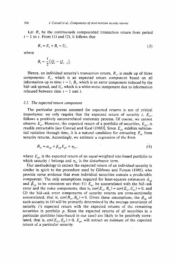
Let R, be the continuously compounded transaction return from period t - 1 to t. From (1) and (2), it follows that

R,=E,+B,+U,, (3)

where

Hence, an individual security’s transaction return, R,, is made up of three components: E,, which is an expected return component based on all information up to time t - 1, B,, which is an error component induced by the bid-ask spread, and U,, which is a white-noise component due to information released between time t - 1 and t.

2.1. The expected 7eturn component

The particular process assumed for expected returns is not of critical importance: we only require that the expected return of security i, Eir, follows a positively autocorrelated stationary process. Of course, we cannot observe Ei,. However, the expected return of a portfolio of securities, Epl, is readily extractable [see Conrad and Kaul (1988)]. Since E,, exhibits substantial variation through time, it is a natural candidate for extracting Ei, from security returns. Accordingly, we estimate a regression of the form

(4)

where EPr is the expected return of an equal-weighted size-based portfolio to which security i belongs and qir is the disturbance term.

Our methodology to extract the expected return of an individual security is similar in spirit to the procedure used by Gibbons and Ferson (1983, who provide some evidence that even individual securities contain a predictable component. The only assumptions required for least-squares estimators GiP and pi, to be consistent are that: (1) EPf be uncorrelated with the bid-ask error and the noise components, that is, cov( Eit, B,,) = cov(Ei,, U,,,) = 0, and (2) the bid-ask error components of security returns are cross-sectionally uncorrelated, that is, cov(Bifr Bj,) = 0. Given these assumptions, the pi, of each security in (4) will be primarily determined by the average covariance of security i’s expected return with the expected returns of the remaining securities in portfolio p. Since the expected returns of all securities in a particular portfolio (size-based in our case> are likely to be positively correlated, that is, cov(&, E,,) > 0, EPr will extract an estimate of the expected return of a particular security.

J. Conrad et al., Components of short-horizon securiry rerurns 369

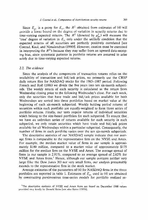
Since EPr is a proxy for E,,, the R’ obtained from estimates of (4) will provide a lower bound on the degree of variation in security returns due to time-varying expected returns. The R’ (denoted by p&> will measure the ‘true’ degree of variation in E,, only under the unlikely condition that the expected returns of all securities are perfectly positively correlated [see Conrad, Kaul, and Nimalendran (1990)]. However, caution must be exercised in interpreting the R”s because they may suffer from an upward data-snoop- ing bias, since systematic patterns in portfolio returns are assumed to arise solely due to time-varying expected returns.

2.2. The ecidence

Since the analysis of the components of transaction returns relies on the availability of transaction and bid/ask prices, we primarily use the CRSP daily return files for NASDAQ stocks for the 1983-1987 period. Following French and Roll (1986) we divide the five years into ten six-month subperiods. The weekly return of each security is calculated as the return from Wednesday closing price to the following Wednesday’s close. For each week, only the securities that have trade and bid/ask prices available for both Wednesdays are sorted into three portfolios based on market value at the beginning of each six-month subperiod. Weekly holding period returns of securities within each portfolio are equally-weighted to form three series of portfolio returns. Finally, our tests require returns of individual securities which belong to the size-based portfolios for each subperiod. To ensure @at we have an unbroken series of returns available for each security in each subperiod, we only retain securities which have trade and bid/ask prices available for all Wednesdays within a particular subperiod. Consequently, the number of firms in each portfolio varies over the ten six-month subperiods.

The descriptive statistics of our NASDAQ sample indicate that our average firms is comparable to the representative firm on the NYSE and Amex. For example, the median market value of firms in our sample is approximately $180 million, compared to a market value of approximately $175 million for the median firm on the NYSE and Amex. The average spread of firms in our sample is 2.91%, compared to an average spread of 2.82% for NYSE and Amex firms.’ Hence, although our sample contains neither very large (like the Dow Jones 30) nor very small firms, our analysis presumably extends to the representative firm in the stock market.

Average estimates of the parameters of (4) for NASDAQ firms in the three portfolios are reported in table 1. Estimates of Epl used in (4) are obtained by constructing parsimonious time-series models for portfolio realized re-

‘The descriptive statistics of NYSE and Amex firms are based on December 1988 values provided very kindly by Donald Keim [see also Keim (198911.

Tab

le

1

Est

imat

es

of

reg

ress

ion

s o

f w

eekl

y in

div

idu

al

secu

rity

tr

ansa

ctio

n

retu

rns

on

p

ort

folio

ex

pec

ted

re

turn

s fo

r N

AS

DA

Q

sto

cks,

Ja

nu

ary

1983

to

D

ecem

ber

19

87.

Th

e re

po

rted

n

um

ber

s ar

e av

erag

e es

tim

ates

o

f re

gre

ssio

n

par

amet

ers

of

ind

ivid

ual

se

curi

ties

b

elo

ng

ing

to

th

ree

po

rtfo

lios

form

ed

by

ran

kin

gs

of

mar

ket

valu

e o

f eq

uit

y o

uts

tan

din

g

at

the

beg

inn

ing

o

f ea

ch

six-

mo

nth

su

bp

erio

d.

Th

e p

aram

eter

s ar

e es

tim

ated

fo

r ea

ch

firm

d

uri

ng

ea

ch ot

’ the

ten

six-

nwnt

l~ su

bp

erio

ds

bet

wee

n

19X

3 an

d

1987

. T

he

ind

ivid

ual

-lir

m

stat

isti

cs

are

aver

aged

ac

ross

fi

rms

wit

hin

ea

ch

po

rtfo

lio

to o

bta

in

suh

per

iod

n

vera

ges

. S

ince

th

e n

um

ber

o

r fi

rms

in e

ach

po

rtfo

lio

vari

es

ove

r th

e te

n

sub

per

iod

s,

ench

re

po

rted

p

aram

eter

es

tim

ate

is t

he

wei

gh

ted

s

gra

nd

av

erag

e o

l’ 11

1e su

bp

erio

d

aver

ages

, w

her

e th

e w

eig

hts

ar

c th

e n

um

ber

o

f lir

ms

in a

po

rtfo

lio

in e

uch

su

bp

erio

d.

Th

e es

tim

ated

re

gre

ssio

n

ia

oc)

N,,

= (?

I,’ +

I-1

,,,&

+

%,.C

’ 5 8

. _.

-.

. I’o

rlfo

lio

&

AZ

h

. 0

I5

lj.3

_~

&I

,;5

B

CX

,,’

l’pc

I’ I

i;,,

R

_~~

_

~_

~_~

..._.

I

-0.0

0121

0.

454

0.05

4 0.

235

0.05

4 o

.otl

2-

- 0.

040

0.07

4 1)

. I I 1

(s

1,1;

rlle

s1)

WO

2)”

(0.1

7.5)

[0

.067

] W

.OS

I)

W.0

78)

WJ5

4)

(O.O

W)

(0.0

55)

6 (0

.051

) ,3

2 -0

.001

34

0.88

1 0.

053

0.22

I

0.03

4 0.

065

- 0.

039

0.0.

5x

0.12

8 8

(0.0

02)

(0.2

00)

[0.0

68]

(0.0

36)

(0.0

81)

(0.0

51)

(0.0

50)

W.O

S5)

(0

.053

) 2

3 -

0.00

042

0.79

1 0.

053

0.19

0 -

0.00

9 0.

082

- 0.

045

0.05

8 0.

152

O

(lar

ges

O

W.0

02)

(0.2

71)

[0.0

661

(0.0

44)

(0.0

73)

(0.0

52)

(0.0

52)

(0.0

54)

(0.0

57)

3 -

~..

~_ _

__

~___

_.~.

. ._

__~

~.~~

._._

_.

~~~

~.

~.

.___

~~

“It,,

= tr

ansa

ctio

ns

retu

rn

ol’

secu

rity

i

for

per

iod

I;

E

,,, =

po

rtfo

lio

exp

ecte

d

retu

rns

for

per

iod

I

thal

ar

e fo

reca

sts

ob

tain

ed

fro

m

AK

(I)

~~~o

dcls

es

tim

utc

d

for

po

rtfo

lio

tran

sact

ion

re

turn

s;

and

v,, =

dis

turb

nn

ce

term

. ‘;

;d,,

= K

2 =

pro

po

rtio

n

of

vari

atio

n

in

real

ized

re

turn

s d

ue

to

the

exp

ecte

d

retu

rn

com

po

nen

t.

Th

e n

um

ber

s in

b

rack

ets

bel

ow

~h

rse

aver

age

esti

mat

es

are

the

aver

age

cro

ss-s

ec’t

ion

al

stan

dar

d

dev

iati

on

s o

f th

e in

div

idu

al-f

irm

st

atis

tics

. C

.. pI

= av

erag

e au

toco

rrel

nti

on

at

lag

k of

th

e ex

pec

ted

re

turn

co

mp

on

ent

of

ind

ivid

ual

se

curi

ty

retu

i-n

s (i

.e.,

the

fitt

ed

valu

es

of

the

esti

mat

ed

reg

ress

ion

s).

All

au

toco

rrel

atio

n

esti

mat

es

are

corr

ecte

d

for

smal

l-sa

mp

le

bia

s b

y ad

din

g

l/(T

-

I),

wh

ere

T

is t

he

nu

mb

er

of

ob

serv

atio

ns

in

a

par

ticu

lar

sub

per

iod

. “T

he

nu

mb

ers

in p

aren

thes

es

bel

ow

th

e g

ran

d

~~ru

ge

esti

mat

es

of

LX

,,,, p

,,,,

nn

d

pk

are

thei

r w

eig

hte

d

stan

dar

d

erro

rs

bas

ed

on

th

e d

istr

ibu

tio

n

of

the

sub

per

iod

av

erag

es.

J. Conrad et al.. Components of short-horizon security returns 371

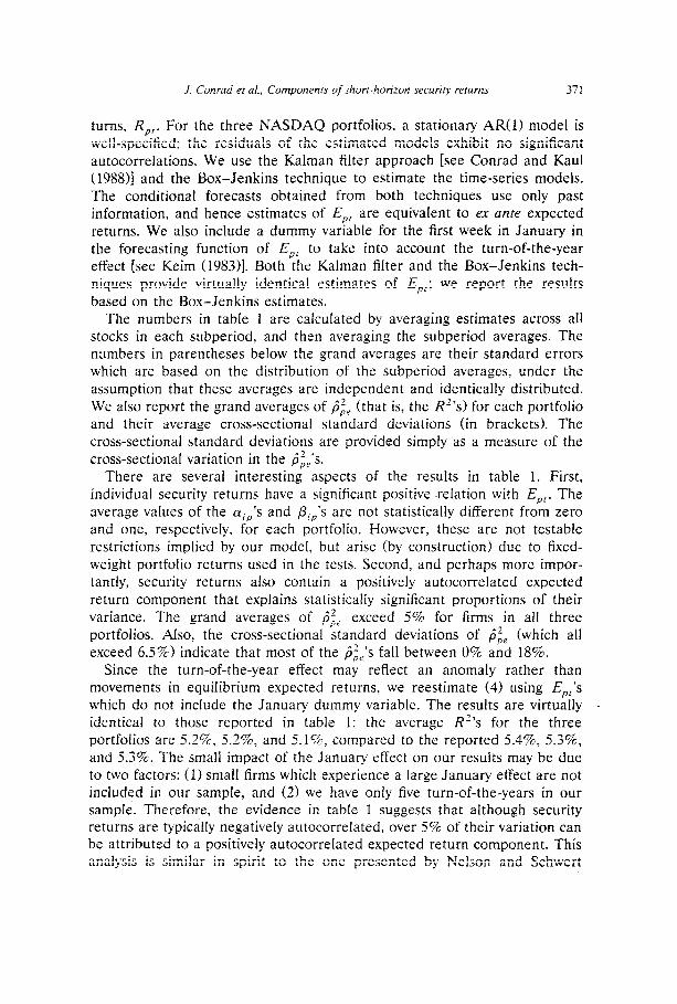
turns, R,,. For the three NASDAQ portfolios, a stationary AR(l) model is well-specified: the residuals of the estimated models exhibit no significant autocorrelations. We use the Kalman filter approach [see Conrad and Kaul (1988)] and the Box-Jenkins technique to estimate the time-series models. The conditional forecasts obtained from both techniques use only past information, and hence estimates of E,, are equivalent to ex ante expected returns. We also include a dummy variable for the first week in January in the forecasting function of E,, to take into account the turn-of-the-year effect [see Keim (1983)]. Both the Kalman filter and the Box-Jenkins techniques provide virtually identical estimates of Ept; we report the results based on the Box-Jenkins estimates,

The numbers in table 1 are calculated by averaging estimates across all stocks in each subperiod, and then averaging the subperiod averages. The numbers in parentheses below the grand averages are their standard errors which are based on the distribution of the subperiod averages, under the assumption that these averages are independent and identically distributed. We also report the grand averages of ci, (that is, the R”s) for each portfolio and their average cross-sectional standard deviations (in brackets). The cross-sectional standard deviations are provided simply as a measure of the cross-sectional variation in the b&-s.

There are several interesting aspects of the results in table 1. First, individual security returns have a significant positive .relation with E,,. The average values of the aiP’s and pip’s are not statistically different from zero and one, respectively, for each portfolio. However, these are not testable restrictions implied by our model. but arise (by construction) due to fixed- weight portfolio returns used in the tests. Second, and perhaps more importantly, security returns also contain a positively autocorrelated expected return component that explains statistically significant proportions of their variance. The grand averages of bj, exceed 5% for firms in all three portfolios. Also, the cross-sectional standard deviations of bi, (which all exceed 6.5%) indicate that most of the ,i$,‘s fall between 0% and 18%.

Since the turn-of-the-year effect may reflect an anomaly rather than movements in equilibrium expected returns, we reestimate (4) using Epr’s which do not include the January dummy variable. The results are virtually identical to those reported in table 1: the average R”s for the three portfolios are 5.2%, 5.2%, and 5.1’72, compared to the reported 5.4%, 5.3%, and 5.3%. The small impact of the January effect on our results may be due to two factors: (1) small firms which experience a large January effect are not included in our sample, and (2) we have only five turn-of-the-years in our sample. Therefore, the evidence in table 1 suggests that although security returns are typically negatively autocorrelated, over 5% of their variation can be attributed to a positively autocorrelated expected return component. This analysis is similar in spirit to the one presented by Nelson and Schwert

372 1. Conrad er al., Components of short-horizon security returns

(1977), who show that although realized real returns on Treasury bills exhibit small autocorrelation coefficients, they can contain a highly autocorrelated expected return component.

Finally, the autocorrelations of the expected returns of firms in each portfolio are presented in the last six columns of table 1. Each autocorrelation estimate is corrected for small-sample bias by adding l/CT- l), where T is the number of observations in a particular subperiod. This correction is exact under the hypothesis that expected returns are serially independent [see Moran (1948)]. The evidence shows that the expected returns of all firms, regardless of market value, are typically positively autocorrelated at all lags. Particularly noteworthy is the strong positive autocorrelation at lag 1. Of course, these autocorrelations simply reflect the autocorrelations of portfolio expected returns, but are reported to demonstrate the likely time-series behavior of the expected returns of individual securities.

We also estimate (4) for securities on the NYSE and Amex. This sample is important because it covers a much longer period, 1962-1985, and therefore we can also estimate monthly regressions. The weekly &‘s range between 2.5% and 4.8%, with the 1970s exhibiting almost twice the degree of variation in Ei,‘s compared to the 1960s and 1980s. More importantly, the monthly

** @$‘s are substantially higher: the average ppe ‘s for small firms is 8.4% for the 1962-1985 period and as high as 17.7% during the 1970s.

2.3. Asymmetry in the predictability of returns

Our sample of NASDAQ stocks also reflects the asymmetry in the predictability of the returns of different size firms uncovered by Lo and Ma&inlay (1990) and Mech (1990). Table 2, panel A, contains the first-order lagged cross-correlations for the three NASDAQ portfolios. The i, jth ele- ment of the correlation matrix is the correlation between Ri.r_, and Rj,t. Note that the elements below the diagonal are larger than those above the diagonal, with the asymmetry being more significant for the largest versus smallest firms.

An appealing property of our methodology for extracting the expected return component is that it is consistent with this intriguing asymmetry displayed by stock returns. Recall that we do not impose an equilibrium model on the expected returns of individual securities. For example, we do not assume a one-factor model [see Lo and Ma&inlay (1990)] and, consequently, do not use the expected return on the market portfolio to extract Ei,‘s of individual securities, without regard to their market values. This procedure would cause expected returns of all securities to be perfectly positively correlated, and all lagged cross-correlations to be symmetric. In- stead, we used expected returns of different size-based portfolios to extract

J. Conrad et al.. Components of short-horizon security returns 373

Table 2

Weekly estimates of first-order lagged cross-correlations between (1) the transaction returns of three equally-weighted portfolios of NASDAQ stocks (panel A) and (2) the residuals of the transaction returns from models in which returns follow a stationary AR(l) process (panel BJ, January 1983 to December 1987. The three portfolios are formed by rankings of market value of equity outstanding at the beginning of each six-month subperiod. Under the hypothesis that the true cross-correlations are zero, the standard error of the estimated cross-correlations is about

0.062.

Variable (x)

Panel A: Return cross-correlationsa

RI, RZl R;,

RI.,-I 0.322 0.235 0.176 R.?.1--1 0.324 0.262 0.196 RI.,- I 0.324 0.273 0.217

Panel B: Residual cross-correlations b

Variable (x)

. ~I.,-, 0.031 0.025 0.020 ELI-1 0.050 0.023 0.01-I E3.1-I 0.067 0.043 0.024

‘R,,, i = 1,2,3. are weekly portfolio transaction returns in week t of the three (smallest to iat&est) portfolios of NASDAQ stocks.

cir, i = 1,2,3. are residuals from weekly estimates of AR(l) models for the transaction returns in week t of the three (smallest to largest) portfolios of NASDAQ stocks.

the expected returns of securities of different market value. This procedure, in turn, takes into account the asymmetric cross-correlations.

Panel B in table 2 reports first-order lagged cross-correlations between the residuals, Elt, from the time-series models for the portfolio returns. Note that the asymmetry is rendered insignificant. This occurs because conditional on a particular (small) portfolio’s own past history of returns, the large portfolio’s return contains little additional information about its future returns. In other words, by construction our portfolio expected returns exhibit the asymmetric lagged cross-correlations witnessed in realized returns. Or course, our procedure does not take into account any asymmetric lagged cross-correlations that may exist between securities within a particular size-based portfolio. However, a more complete model for expected returns of individual securities is beyond the scope of this paper.

2.4. The bid-ask error component

Based on our model for security prices in (1) and (21, the bid and ask prices, BPi, and APit, of security i may be written as

BPi, = Pi, - ;Qit

373

and

J. Conrad er al., Components of short-hori:on security returns

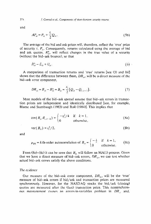
The average of the bid and ask prices will, therefore, reflect the ‘true’ price of security i, P,!. Consequently, returns calculated using the average of bid and ask quotes, R;!, will reflect changes in the true value of a security (without the bid-ask bounce), so that

R:, = Ei, -t U,,. (6)

A comparison of transaction returns and ‘true’ returns [see (3) and (611 shows that the difference between them, DR,,, will be a direct measure of the bid-ask error component,

w, = Rr (7)

Most models of the bid-ask spread assume that bid-ask errors in transaction prices are independent and identically distributed [see, for example, Blume and Stambaugh (1983) and Roll (19&I)]. This implies that

cov( Bit B;.r_k) = -s2/4 if ’ = ‘, 0 otherwise,

(84

var( Bj,) = $/2, (8b)

and

pBk = k th-order autocorrelation of Bit = i

- t if k=l,

0 otherwise. (8~)

From (8a)-(Sc) it can be seen that Bi, will follow an MA(l) process. Given that we have a direct measure of bid-ask errors, DR,,, we can test whether actual bid-ask errors satisfy the above conditions.

The ecidence

Our measure of the bid-ask error component, DR,,, will be the ‘true’ measure of bid-ask errors if bid/ask and transaction prices are measured synchronously. However, for the NASDAQ stocks the bid/ask (closing) quotes are measured after the (last) transaction price. This nonsynchronous measurement causes an errors-in-variables problem in DR,, and,

J. Conrad er al., Components of short-horizon m-wiry returns 375

Table 3

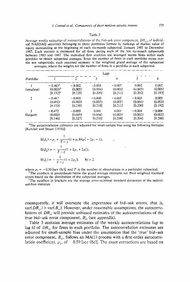
Average weekly estimates of autocorrelations of the bid-ask error component, DR,,, of individual NASDAQ securities belonging to three portfolios formed by rankings of market value of equity outstanding at the beginning of each six-month subperiod. January 1983 to December 1987. Each statistic is estimated for all firms during each of the ten six-month subperiods between 1983 and 1987. The individual firm statistics are averaged across firms within each portfolio to obtain subperiod averages. Since the number of firms in each portfolio varies over the ten subperiods, each reported estimate is the weighted grand average of the subperiod

averages, where the weights are the number of firms in a portfolio in each subperiod.

Lags

Portfolio 1 2 3 4 5 6

1 (smallest)

- 0.463” (0.003)b [O. 1521=

2 - 0.467 (0.002) IO. 1531

3 (largest)

-0.472 (0.003) LO.1461

- 0.002 (0.005) i0.2251

- 0.003 (0.003) [0.2301

- 0.003 (0.005) IO.2271

- 0.003 (0.004) [0.209]

- 0.000 (0.003) [0.2181

0.001 (0.004J LO.2 161

-0.007 (0.003) lo.21 11

- 0.005 (0.005) LO.21 11 0.001

(0.003) [0.2091

0.002 (0.003) [0.2021

-0.003 (0.004) [0.2001

-0.004 (0.002) [0.2041

0.002 (0.009 lO.1931

0.005 (0.003) fO.1921

-0.000 (0.002, [@.2001

aThe autocorrelation estimates are adjusted for small-sample bias using the following formulas [Kendall and Stuart (1976)]:

E(p^,J=p, + &,I +/?,X4pf - 2p, - I), -.

EC&) = - AU +2&J, + 2pfJ,

E(sji) = - &I + 2p,), vj > 2,

where p, = -0.50 [see (8~11, and T is the number of obsemations in a particular subperiod. bThe numbers in parentheses below the grand average estimates are their weighted standard

errors based on the distribution of the subperiod averages. ‘The numbers in brackets are the average cross-sectional standard deviations of the individ-

ual-firm statistics.

consequently, it will overstate the importance of bid-ask errors, that is, var(DRi,) > var(Bj,). However, under reasonable assumptions, the autocorrelations of DR,, will provide unbiased estimates of the autocorrelations of the true bid-ask error component, II,, (see appendix).

Table 3 contains average estimates of the weekly autocorrelations (up to lag 6) of DR,, for firms in each portfolio. The autocorrelation estimates are adjusted for small-sample bias under the assumption that the ‘true’ bid-ask error component, Bit, follows an MA(l) process with a first-order autocorre- latidn coefficient, pt, of -0.50 [see (SC)]. The exact corrections are based on

376 .I. Conrad et al.. Components of shorr-horizon security returns

the following equations [Kendall and Stuart (197611:

E(6,) =PI + &Cl +p1)(4pi? - 2P, - I>, (9a)

E(&) = -L( T-2

1+ 2p, + 2p3, (9b)

E(b,) = - ‘dj>3.

The estimated autocorrelations in table 3 are generally consistent with the model and assumptions for Bi,. The average first-order autocorrelations of DRi, are similar across all portfolios, and range between - 0.463 and - 0.472. All higher-order autocorrelations are small in magnitude. There is some evidence that bid-ask errors in transaction prices may not be independently distributed; the first-order autocorrelations are statistically less than 0.50 in absolute magnitude, and higher-order autocorrelations are occasionally significantly different from zero. However, the correlation in bid-ask errors in transaction prices appears to be small, and DRi, closely approximates an MA(l) process.

3. Properties of individual security returns

In this section, we present estimates of the degree of variation in NASDAQ weekly security returns that can be attributed to the three uncorrelated components: Eir, B,,, and Ui,. We also present evidence that recon- ciles the contrasting time-series behavior of short-horizon security and portfolio returns.

3.1. Components of security returns

Table 4 contains estimates of the proportions of variance of NASDAQ weekly security returns explained by the adjusted bid-error component, the expected return component, and the noise component. The contribution of the bid-ask error component, Bit, to return volatility is calculated as var(DR,>/var(R,,>, and is denoted by c$.’ The proportion of return vari-

pph overstates the importance of bid-ask errors in transaction returns because bid/ask quotes are measured after transaction prices. However, since the denominator of this ratio measures the variance of weekly transaction returns, the upward bias in si, is likely to be small

[see appendix]. Also, bz, is calculated under the assumption that all trades occur either at the

bid or the ask quote. If trades occur within the spread, var(DR,,). and hence G$,, will overstate the importance of bid-ask errors. However, according to NASD dealers, trades within the quoted spread are infrequent and form only a small percentage of total trades in NASDAQ stocks.

J. Conrad et al., Components of short-horizon security returns 377

Table 4

Average weekly estimates of the proportions of variance of NASDAQ individual security transaction returns explained by the bid-ask error component, P$,, the expected return component. pi,, and the noise component. pi,,. January 1983 to December 1987. The average estimates are of securities belonging to three portfolios formed by rankings of market value at the beginning of each six-month subperiod. Each statistic is estimated for all firms during each of the ten &u-month subperiods between 1983 and 1987. The individual-firm statistics are averaged across firms within each portfolio to obtain subperiod averages. Since the number of firms in each portfolio varies over the ten subperiods. each reported estimate is the weighted grand average of the subperiod averages, where the weights are the number of firms in a portfolio in

each subperiod.”

1 0.190 0.054 0.756 (smallest) (0.014)” to.004, (0.016)

[O. 1761’ [0.067] [O. 1701

2 0.114 0.053 0.833 (0.007) (0.005) (0.009) [0.1161 [0.068] [0.132]

3 0.058 0.053 0.889 (largest) (0.003) (0.004) (0.005)

[0.083] [0.0661 [O. 1081

‘b$, = var(DR,,)/var(R,,) = proportion of variation in realized security returns due to the bid-ask error component; bfr = R’ (of regression in table 1) = proportion of variation in realized returns due to the expected return component: and p^z,, = 1 - bzC - fi$, = proportion of variation in realized returns caused by the noise component.

‘The numbers in parentheses below the grand average estimates are their weighted standard errors based on the distribution of the subperiod averages.

‘The number in brackets are the averaged cross-sectional standard deviations of the individual-firm statistics.

ante explained by the expected return component, bie, is simply the R2 from estimates of (4). Finally, we obtain an estimate of the degree of variation in returns due to the noise component as Gi,, = 1 -&, -b$,.

Table 4 shows that bid-ask errors induce a large degree of spurious volatility in weekly transaction returns. Average estimates of & range between 5.8% for large firms and 19.0% for small firms. The average cross-sectional standard deviations are also large, ranging between 8.3% and 17.6%. Hence, for the small firms in our sample, between 0% and 54.2% of return volatility can typically be explained by the bid-ask error component. The proportions of return variance explained by B,, are also significantly larger than the proportions (of about 5%) induced by time-varying expected returns, especially for small firms. Finally, the predominant source of variation in security returns is the arrival of new information. Estimates of the proportion of return variance explained by the rational information component range between 75.6% and 88.9 %. These larger proportions support the

378 J. Conrud et al.. Components of short-horizon security returns

evidence in French and Roll (1986) and Barclay, Litzenberger, and Warner (1990).

The relative importance of the three components of most (except the very small and very large) NYSE and Amex security returns is likely to be similar to the estimates in table 4. As noted earlier, the average quoted bid-ask spread of all firms in our sample is 2.914%, which compares favorably with the average spread of 2.817% for NYSE and Amex firms at the end of 1988. Since the spurious volatility generated by the bid-ask error component is directly related to the square of the spread [see (8b)], the importance of the bid-ask error component for the average NYSE and Amex firm is also likely to be nontrivial.

3.2. Reconciliation of the time-series behacior of indicidual security and portfolio returns

Given our model for security returns in (3) and the properties of the three components, reconciling the negative autocorrelation in security returns with the positive autocorrelation in portfolio returns is fairly straightforward. Without loss of generality, consider, for example, the first-order autocorrelation, pi, of an individual security’s transaction return

‘OVtEflqEi,t-,) +CoV(BittB,.r-I) P, =

W R,,) ( 10)

From (IO) it follows that the sign of the first-order autocorrelation depends on the relative magnitudes of the autocovariances generated by the expected return and the bid-ask error components. respectively. In particular,

p,$O iff /COV(Eit~Ei,r-~)[$[CoV(Bir~Bi,,-,)(’ (11)

The fact that the positive autocovariance generated by the expected return component is not typically discernible in the case of short-horizon security returns implies that it is contaminated by the larger negative autocovariance induced by the bid-ask error components. Of course, this need not be the case for every security. For example, the daily first-order autocorrelations of larger firms tend to be positive, though small in magnitude [Fama (1965) and French and Roll (1986)]. These findings are also consistent with our mode1 because the autocovariance generated by bid-ask errors is likely to be smaller for larger firms, since such firms have smaller spreads [see (Sa>].

Roll (1984) and Amihud and Mendelson (1987) conjecture similar explana- tions for their unrealistically low spread estimates based on the first-order

J. Conrud et ul., Componer~s of short-hori:on security returns 379

autoco;/ariance of transaction returns. Both studies assume that the expected return of a security is constant, and find that the negative first-order autocovariance is much smaller (in absolute magnitude) than that implied by the bid-ask bounce, that is, Icov(Ri,, R,,, t _ i )I < s3/4 [see (8a>l. Roll conjectures that a positively autocorrelated expected return process could be responsible for this result. Amihud and Mendelson argue that daily return autocovari- antes could be small because of partial price adjustments induced by smooth- ing effects by market makers. However, the effects of such adjustments are likely to be dissipated over intervals as Ion, 0 as a week (the measurement interval used in this paper) [see Amihud and Mendelson (1987)I.

We use two related tests to gauge the ability of our model to explain the differing time-series properties of individual security and portfolio returns. The first test compares the autocovariances of transaction returns with the sum of the autocovariances of our proxies for expected returns and the bid-ask error component, that is, &(R,,, Ri.t_i)’ versus c8v(Ei,, E,,,_j) + c&(DR,,, DR,,,_;). If our model is the correct specification of the return generating process, these two estimates should be equal. However, caution must be exercised in making such comparisons since the cross-sectional averages of c&C&, Ei,!_, 1 are likely to be downward biased because they measure cov( Ept, E,,,_ , ), which is the average of cov( Ejt, E,,,_ , ), i # j. Also, it is likely that the average of the true autocovariances, cov(Eit, Ej,t_I), is larger than the average of cov(Eirt E,.,_ ,). Hence, we evaluate these estimates for general patterns, without placin g undue emphasis on the exact magnitudes of c&(R,,, R,,l_j) versus cME,,, Ei.t_j) + ciXDR,,, DR,,,_j).

For brevity we do not report the results, but the evidence suggests that our model is broadly consistent with most of the time-series properties of security and portfolio returns. First, our model can explain the positive first-order autocorrelation of portfolio returns versus the typically negative first-order autocorrelation in security returns. The average first-order autocovariance generated by the bid-ask error component is always larger in (absolute) magnitude than the autocovariance generated by the expected return component. Second, although our measure of Ej, is an imperfect proxy, the patterns in its autocovariances are similar to those in the autocovariances of Ri,. For example, both R,, and E,, reflect significant autocovariances at lags 5 and 6 but, consistent with our earlier conjecture, c&(E,,, Ei.r_j) < c6v(Ri,, Ri.r_il The only systematic characteristic of the time-series behavior of transaction returns that is inconsistent with our model are the statistically significant (but small) negative autocovariances at lag 2.

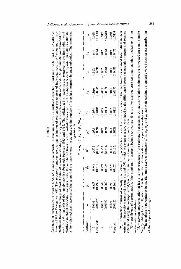
The second test is a specification test which also helps us evaluate our model’s ability to explain the contrasting time-series behavior of security and portfolio transaction returns. Since we have proxies for both the expected return component, Ei,, and the bid-ask error component, B,,, we estimate

380 J. Conrad et al.. Components of short-horizon security returns

the following regression:

R,t = ai + P,iEit + PziBit + tic. ( 12)

The autocorrelations of the residuaIs of (1.2) provide a direct test of whether our model captures all of the components of security returns. If our model is a valid characterization of security returns, the residuals should behave like white noise, thus explaining the differing characteristics of security and portfolio returns. If bid/ask quotes and transaction prices are measured at the same time, DRi, would be a perfect measure of B,, and, by definition, pzi = 1 for each security. However, due to the nonsynchronous measurement of transaction and bid/ask prices, var( DRi,) > var( Bi, 1, and & will be asymptotically downward biased. We nevertheless estimate (12) to gauge the specification of our model.

The average estimates of the parameters of (12) in table 5 show the downward bias in p^, and, as expected (see appendix), the bias is larger for larger firms. The residual autocorrelations reveal ‘unexplained’ patterns that are virtually identical to the autocovariance analysis of Ril, Eit, and DRi, discussed above. After accounting for time-varying expected returns and bid-ask errors, there remains some significant negative autocorrelation at lag 2 and significant positive autocorrelations at lags 1, 5, and 6. The positive autocorrelations at lags 1, 5, and 6 are perfectly consistent with our model, and are a consequence of using an imperfect proxy, Ept, to extract Ei,. On the other hand, as indicated earlier, the negative autocovariance/autocorrelation at lag 2 is not consistent with our model, especially since the bid-ask error component closely approximates an MA(l) process. However, the average magnitudes of these autocorrelations are small, ranging between -0.025 and -0.047. Therefore, although our model does not capture all components which could potentially lead to negative autocorrelations in security returns (such as nonsynchronous trading, price discreteness, and/or market overreaction), it is unlikely that these components play an important role in the determination of ‘observed’ prices. Bid-ask errors appear to be the major source of negative autocorrelation in security returns.

Having established that individual security returns (though usually negatively autocorrelated) do contain a positively autocorrelated common component, our model can be readily used to explain the strong positive autocorrelation in portfolio returns. The return of a portfolio containing a large number of securities wiIl exhibit strong positive autocovariance because bid-ask errors are cross-sectionally uncorrelated, and are diversified away in the portfolio formation process. Diversification also causes the variances of portfolio returns to be much smaller than the variances of security returns: for example, the variance of the returns of portfolio 1 is less than one-tenth

Eslim

ate

s o

f re

gre

ssio

ns

of

we

ek

ly

NA

SDA

Q

ind

ivid

ua

l se

cu

rhy

tr

un

suc

tion

re

turn

s o

n

po

rtfo

lio

exp

ec

ted

re

turn

a

d

the

h

id-a

sk

err

or

vnria

ble

, Ja

nu

ary

1’

983

IO D

ec

em

be

r 19

87.

The

re

po

rte

d

nu

mb

ers

a

re

ave

rag

e e

stim

ate

s o

f re

gre

ssio

n

pa

ram

ete

rs

of

ind

ivid

ua

l sc

cu

ritirs

b

elo

ng

ing

to

th

ree

po

rtfo

lios

form

ed

b

y ra

nk

ing

s o

f tn

ark

et

valu

e o

f e

qu

ity

ou

tsta

nd

ing

a

t th

e b

eg

inn

ing

o

f e

ac

h s

ix-m

on

th

sub

pe

riod

. Th

e

pa

ram

ete

rs

are

est

imn

td

for

each

fir

m

du

ring

e

ac

h o

f th

e

ten

six

-mo

nth

su

bp

erio

ds

be

twe

en

10

83 a

nd

19

87.

The

in

div

idu

al-

firm

st

atis

tics

are

ave

rag

ed

ac

ross

tir

ms

with

in

ea

ch

po

rtfo

lio

lo o

bta

in

sub

pe

riod

a

vera

ge

s. S

inc

e

the

nu

mb

er

of

firm

s in

ea

ch

po

rtfo

lio

varie

s o

ver

the

te

n s

ub

pe

riod

s,

ea

ch

re

po

rte

d

pa

ram

ete

r &

ma

le

is

the

we

igh

ted

g

ran

d

ave

rag

e o

f th

e s

ub

pe

riod

a

vera

ge

s, w

he

re

the

we

igh

ts

are

th

e n

um

be

r o

f tir

ms

in a

po

rtfo

lio

in e

nc

h s

ub

pe

riod

. Th

e

est

imu

tctl

reg

ress

ion

is

R,,

= (

Y,

+

PI,

E,,,

+ /

j2,

DR

,, +

q,,.”

R2

I,

A

I -

0.00

2 0.

883

0.X

46

0.23

2 0.

032

- 0.

034

-0.0

16

0.00

2 0.

004

0.0

IX

(slll

;lllL

’st)

(O

.m)”

(0

. I 0

9)

(0.0

1h)

10. I

7SI

(0.0

09)

(O.O

lO)

WO

O4)

w

nr))

~0.0

06)

wcn

bx)

2 -

0.00

2 0.

948

0.77

7 0.

177

0.0

I2

- 0.

025

- 0.

007

- 0.

002

0.01

2 O

.OI 7

(0.0

02)

(0.2

02)

(0.0

26)

[0.1

441

(0.0

09)

(0.0

I I

)

U~

.OO

7)

(0.0

06)

W.O

O~

d

W.0

10)

3 -

0.00

1 0.

894

0.67

4 0.

I37

0.

023

- 0.

047

-0.0

1 1

-0.0

14

0.01

9 0.

030

(la

rge

st)

UL0

02)

(0.2

69)

(0.0

26)

(0.1

221

(0.0

12)

(0.0

12)

(0.0

07)

U~

.008

) (0

.007

) W

.01S

) -.

-~_I

__

____

__~

-

- .~

~__

_.__

“It,,

=

tr

imsi

tctio

n

relu

rns

of

st‘c

urit

y

i in

p

erio

d

I; E,

,, =

p

ort

folio

e

xpe

cte

d r

etu

rns

for

pe

riod

I

tha

t a

re

fore

ca

sts

ob

tain

ed

fr

om

A

R(l

) m

od

els

est

im;it

ctl

for

po

rtfo

lio

tra

nsa

ctio

n

retu

rns;

an

d D

R,,

= h

id-a

sk

err

or

me

asu

re

ca

lcu

late

d

as

the

di!I

’ere

nc

e

be

twe

en

tr

an

sac

tion

re

turn

s a

nd

re

lurn

s c

alc

ula

ted

u

sin

g

the

a

vera

ge

of

bid

/ask

p

rice

s,

an

d

v,,

=

ran

do

m

tlisl

urb

an

ce

te

rm.

“I?

= c

oe

tlic

ien

t o

f c

lete

rmim

itio

n.

The

n

um

be

rs

in

hra

ck

rts

be

low

th

e

ave

rag

e

12”s

a

re

the

a

vera

ge

cro

ss-s

ec

tion

al

sta

nd

ard

d

evi

atio

ns

of

the

in

tlivi

du

ul-

lirm

st

atis

lics.

‘!;

A =

avc

rug

e ~

iulo

co

rre

latio

n

at

lag

k o

f ~

hr

resi

du

als

o

f th

e e

stim

ate

d

reg

ress

ion

s.

All

au

toc

orr

ela

\io

n

esl

ima

tes

arc

co

rre

cte

d

for

sma

ll-sn

mp

le

bitt

s b

y a

dd

ing

I/

(?‘-

I)

, w

he

re

7‘ i

s th

e

nu

mb

er

of

ob

serv

atio

ns

in

:I p

art

icu

lar

sub

pe

riod

.

“Th

e

nu

mb

ers

in

pa

ren

the

ses

be

low

th

e g

ran

d

ave

rag

e e

stim

ate

s o

f (Y

, /3,

, /3

?, a

nd

pI.

are

th

eir

we

igh

ted

st

~m

dm

d

err

ors

b

ase

d W

I th

e d

istr

ibu

tion

of

the

su

hp

erio

d

ave

rag

es.

382 J. Conrad et al.. Components of short-horizon secunty rerurns

the average variance of the returns of its constituent securities. The combina- tion of these two factors leads to strong positive autocorrelation in portfolio returns.

4. Summary and conclusions

In this paper, we present a simple three-component model for security returns that appears to capture the important time-series characteristics of short-horizon returns. Specifically, an individual security’s return is assumed to be made up of three independent components: a positively autocorrelated expected return component, a negatively autocorrelated component induced by bid-ask errors, and a white-noise component.

We introduce a methodology to extract the ‘unobsetvable’ expected return and bid-ask error components of individual security returns, and show that these components explain substantial proportions of the variance of transaction returns - between 11% and 24% of the degree of variation in weekly transaction returns. We also reconcile the negative autocorrelation in individual security returns with the strong positive autocorrelation displayed by portfolio returns, and show that our measures of the expected return components of large versus small firms reflect the asymmetric lagged cross-correlations documented by Lo and Ma&inlay (1990) and Mech (1990).

Appendix: Measurement errors in the bid-ask error variable

Recall that our bid-ask error measure, DR,,, suffers from a nonsynchronous measurement problem because bid/ask quotes are typically measured after the transaction price. Consequently, ‘measured’ DR,, can be written as

DR;, = Ri, - R;l = Bit + L,,,_ , - Lit, (A-1)

where Li, is the component of ‘true’ return (without the bid-ask error), that is, RF,, measured over the nontrading interval between the last transaction and market close on day t.

Suppose Lit is identically distributed for a particular security [see Scholes and Williams (197711. From (A.11 it follows that DR,, will be a noisy measure of Bit since var( DR,,) = var(Bi,) + 2var(L,,) =x,2/2 + 2var(L,,) [see (8b>].3 Hence, var(DR,,) will overstate the importance of bid-ask errors in transaction returns. Although 2var(L,,) will be small compared to the variance of

‘The expression for var(DR,,) is derived under the additional assumption that L,,is independently distributed. This is a reasonable assumption because Lil’s are measured over small intervals that are one week apart.

J. Conrad et al., Cmqxments of short-horizon security returns 383

‘true’ weekly returns, RLIL:, it may be large relative to var(B,,), which is given by sf/2, where si is the spread of security i. The average values of s”/2 for the three NASDAQ portfolios are (approximately) 0.00136, 0.00049, and 0.00013. Hence, especially for large firms, measurement errors in DR,, could have potentially important implications for specification tests of our model.

Given the assumptions about the ‘true’ bid-ask error component [see (XaMSc)], and the returns measured over the nontrading intervals, L,,, it can be shown that

COV(~~ir,~~i,,_,) = -S2/4-var(Lit) if k=17 0 otherwise,

(A.?)

and the k th-order autocorrelation of DR,,, pk, is

if k=l,

otherwise. (A.3)

From (A.2) and (A.3) it follows that although the first-order autocovari- ante of DR,, will provide an upward-biased (in absolute magnitude) estimate of cov(B,,, B,.,_,), all its autocorrelations (including p,) will be unbiased estimates of the autocorrelations of the ‘true’ bid-ask error component, Bit.

References

Amihud. Yakov and Haim Mendelson, 1987, Trading mechanisms and stock returns: An empirical investigation, Journal of Finance 42. 533-553.

Barclay, Michael J., Robert H. Litzenberger. and Jerold B. Warner, 1990. Private information. trading volume, and stock return variances, Review of Financial Studies 3. 233-353.

Blume, Marshall E. and Robert F. Stambaugh. 1983, Biases in computed returns: An application to the size effect, Journal of Financial Economics 12, 387-404.

Conrad. Jennifer and Gautam Kaul. 1988, Time-variation in expected returns. Journal of Business 61, 409-425.

Conrad, Jennifer and Gautam Kaul, 1989, Mean reversion in short-horizon expected returns. Review of Financial Studies 2, 225-240.

Conrad, Jennifer and Gautam Kaul, 1991, Frictions and the time series properties of asset returns, Working paper (University of Michigan. Ann Arbor, MI).

Fama. Eugene F.. 1965, The behavior of stock market prices. Journal of Business 38. 34-105. Fama. Eugene F., 1976, Foundations of finance (Basic Books, New York, NY). French, Kenneth R. and Richard Roll, 1986, Stock return variances: The arrival of information

and the reaction of traders, Journal of Financial Economics 17. j-26. Gibbons, Michael R. and Wayne Ferson, 1985, Testing asset pricing models uith changing

expectations and an unobservable market portfolio. Journal of Financial Economics l-1, 217-236.

Kaul. Gautam and M. Nimalendran, 1990. Price reversals: Bid-ask errors or market overreaction’?, Journal of Financial Economics. forthcoming.

Keim. Donald B.. 1983. Size-related anomalies a-nd stock return seasonality: Further empirical evidence. Journal of Financial Economics 12, 13-32.

Keim. Donald B.. 1989. Trading patterns, bid-ask spreads and estimated security returns: The case of common stocks at calendar turning points, Journal of Financial Economics 25, 75-97.

384 J. Conrad et al., Components of short-hori:on security returns

Kendall, Maurice G. and Alan Stuart, 1976, The advanced theory of statistics. Vol. 3 (Griffin, London).

Lo. Andrew and A. Craig Ma&inlay, 1988, Stock market prices do not follow random walks: Evidence from a simple specification test, Review of Financial Studies 1, 41-66.

Lo, Andrew and A. Craig Ma&inlay, 1990, When are contrarian profits due to stock market overreaction?, Review of Financial Studies 3, 175-205.

Mech. Timothy S., 1990, The economics of lagged price adjustment. Working paper (Boston College, Boston. MA).

Moran. P.A.P., 1948. Some theorems on time series. Biometrika 35. 255-260. Nelson. Charles R. and G. William Schwert. 1977, Short-term interest rates as predictors of

inflation: On testing the hypothesis that the real rate of interest is constant, American Economic Review 67, 665-678.

Roll, Richard, 1984, A simple implicit measure of the effective bid-ask spread in an efficient market, Journal of Finance 39, 1127-l 139.

Scholes. Myron and Joseph Williams, 1977, Estimating betas from nonsynchronous data, Journal of Financial Economics 5. 309-327.

components of short-horizon individual security returns

Documents