Component-based Car Detection

in Street Scene Images

by

Brian Leung

Submitted to the Department of Electrical Engineering and ComputerScience

in partial fulfillment of the requirements for the degree of

Master of Engineering in Computer Science and Electrical Engineering

at the

MASSACHUSETTS INSTITUTE OF TECHNOLOGY

May 2004

c© Brian Leung, MMIV. All rights reserved.

The author hereby grants to MIT permission to reproduce anddistribute publicly paper and electronic copies of this thesis and to

grant others the right to do so.

Author . . . . . . . . . . . . . . . . . . . . . . . . . . . . . . . . . . . . . . . . . . . . . . . . . . . . . . . . . . . . . .Department of Electrical Engineering and Computer Science

May 20, 2004

Certified by. . . . . . . . . . . . . . . . . . . . . . . . . . . . . . . . . . . . . . . . . . . . . . . . . . . . . . . . . .Tomaso Poggio

Eugene McDermott ProfessorThesis Supervisor

Accepted by . . . . . . . . . . . . . . . . . . . . . . . . . . . . . . . . . . . . . . . . . . . . . . . . . . . . . . . . .Arthur C. Smith

Chairman, Department Committee on Graduate Students

2

Component-based Car Detection

in Street Scene Images

by

Brian Leung

Submitted to the Department of Electrical Engineering and Computer Scienceon May 20, 2004, in partial fulfillment of the

requirements for the degree ofMaster of Engineering in Computer Science and Electrical Engineering

Abstract

Recent studies in object detection have shown that a component-based approachis more resilient to partial occlusions of objects, and more robust to natural posevariations, than the traditional global holistic approach. In this thesis, we considerthe task of building a component-based detector in a more difficult domain: cars innatural images of street scenes. We demonstrate reasonable results for two differentcomponent-based systems, despite the large inherent variability of cars in these scenes.

First, we present a car classification scheme based on learning similarities to fea-tures extracted by an interest operator. We then compare this system to traditionalglobal approaches that use Support Vector Machines (SVMs). Finally, we presentthe design and implementation of a system to locate cars based on the detections ofhuman-specified components.

Thesis Supervisor: Tomaso PoggioTitle: Eugene McDermott Professor

3

4

Acknowledgments

First, I would like to thank Tommy for being such a patient and understanding thesis

advisor. His foresight, intuition, and care were instrumental in shaping this work. I

want to thank rif for his role as both a teacher and an advisor. He taught me how

to dig deeper and provided me with the guidance I needed to get started. I thank:

Stan, for his insights and intuition in the subject matter of this thesis. Lior, for his

seemingly infinite supply of ideas and new avenues of research to pursue. I must

thank Tommy again for letting me work with such great researchers. Lastly, I thank

my family whose hard work and sacrifice made this thesis even possible.

If I may, I would also like to take this moment to thank the many great teachers,

mentors, managers, advisors, and friends that I have had the pleasure to interact with

over the past 5 years.

Much of the work in this thesis is joint work with various members of CBCL. The

work in Chapter 3 of this thesis is joint work with Stanley Bileschi and Ryan Rifkin.

The work in Chapter 4 is joint work with Lior Wolf.

5

6

Contents

1 Introduction 13

1.1 Problem Statement . . . . . . . . . . . . . . . . . . . . . . . . . . . . 14

1.2 Motivation . . . . . . . . . . . . . . . . . . . . . . . . . . . . . . . . . 15

1.3 Outline of Thesis . . . . . . . . . . . . . . . . . . . . . . . . . . . . . 17

2 Object Detection 19

2.1 Object Classifier . . . . . . . . . . . . . . . . . . . . . . . . . . . . . 20

2.1.1 Statistical Learning Framework . . . . . . . . . . . . . . . . . 20

2.1.2 Feature Spaces . . . . . . . . . . . . . . . . . . . . . . . . . . 23

2.1.3 Global Approaches . . . . . . . . . . . . . . . . . . . . . . . . 24

2.1.4 Component-based Approaches . . . . . . . . . . . . . . . . . . 24

2.2 Object Detection Framework . . . . . . . . . . . . . . . . . . . . . . . 25

2.3 Miscellaneous . . . . . . . . . . . . . . . . . . . . . . . . . . . . . . . 26

3 Hierarchical Car Classifier using an Interest Operator 29

3.1 Interest Operator and SIFT Feature Descriptor . . . . . . . . . . . . 30

3.2 Keypoint-based Car Detector . . . . . . . . . . . . . . . . . . . . . . 31

3.3 Experiments . . . . . . . . . . . . . . . . . . . . . . . . . . . . . . . . 32

3.3.1 Databases . . . . . . . . . . . . . . . . . . . . . . . . . . . . . 32

3.3.2 Global (Non-hierarchical) SVM Classifiers - A survey of feature

spaces . . . . . . . . . . . . . . . . . . . . . . . . . . . . . . . 34

3.3.3 Keypoint-based Car Detector . . . . . . . . . . . . . . . . . . 37

3.4 Discussion . . . . . . . . . . . . . . . . . . . . . . . . . . . . . . . . . 41

7

4 Component-based Approach 43

4.1 System Architecture . . . . . . . . . . . . . . . . . . . . . . . . . . . 43

4.1.1 Component Detection . . . . . . . . . . . . . . . . . . . . . . 44

4.1.2 Component Combination . . . . . . . . . . . . . . . . . . . . . 47

4.1.3 Car Detection . . . . . . . . . . . . . . . . . . . . . . . . . . . 48

4.2 Experiments . . . . . . . . . . . . . . . . . . . . . . . . . . . . . . . . 49

4.2.1 Database . . . . . . . . . . . . . . . . . . . . . . . . . . . . . 49

4.2.2 Component Detectors . . . . . . . . . . . . . . . . . . . . . . . 50

4.2.3 Component Combination Classifiers . . . . . . . . . . . . . . . 50

4.2.4 Car Detection . . . . . . . . . . . . . . . . . . . . . . . . . . . 51

4.3 Discussion . . . . . . . . . . . . . . . . . . . . . . . . . . . . . . . . . 56

5 Conclusion 59

5.1 Comparison with Prior Work in Car Detection . . . . . . . . . . . . . 60

6 Future Work 63

6.1 Derivative Work . . . . . . . . . . . . . . . . . . . . . . . . . . . . . . 63

6.2 More Objects . . . . . . . . . . . . . . . . . . . . . . . . . . . . . . . 64

6.3 Context and Segmentation . . . . . . . . . . . . . . . . . . . . . . . . 64

6.4 Object Identification and Categorization . . . . . . . . . . . . . . . . 65

8

List of Figures

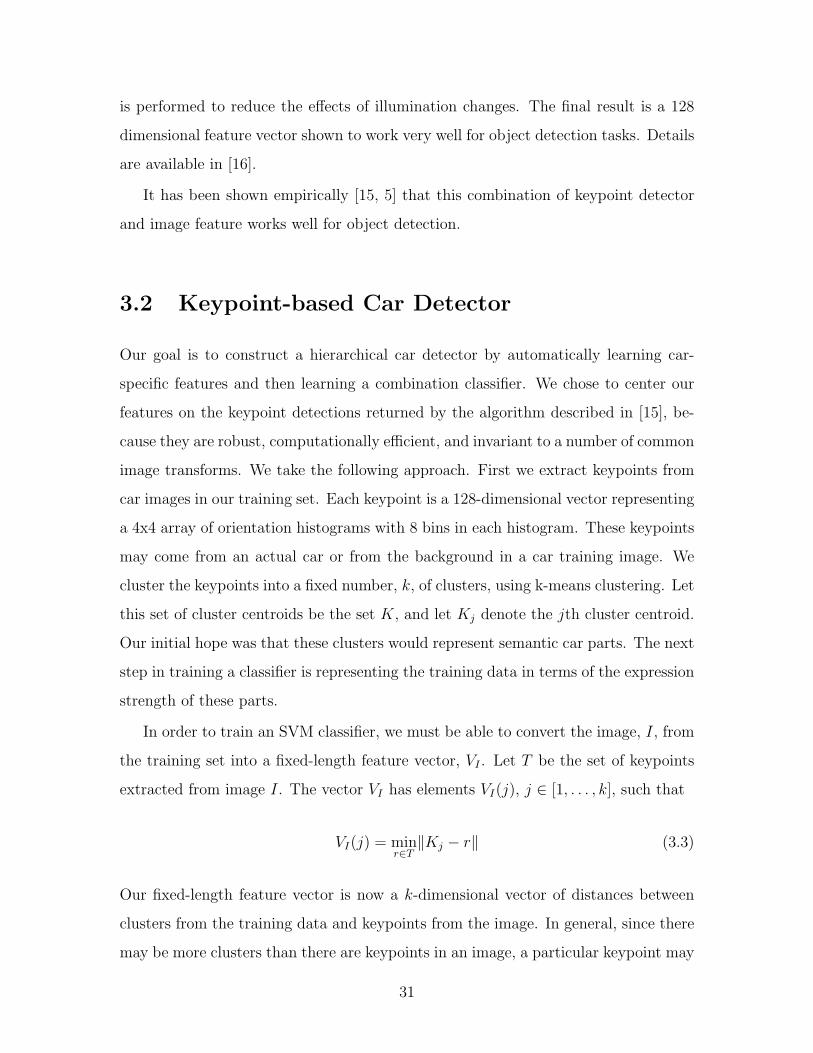
3-1 Examples of cars and non-cars from the training and test set in the

Modified UIUC Image Database for Car Detection. All car images are

side views of cars where the car is spatially localized in the image.

The first and third row are examples of positive and negative training

images. The second row contains the crops from the test images of

the UIUC Image Database; these images were used as our positive test

images. The last row contains examples of negative test images. . . . 33

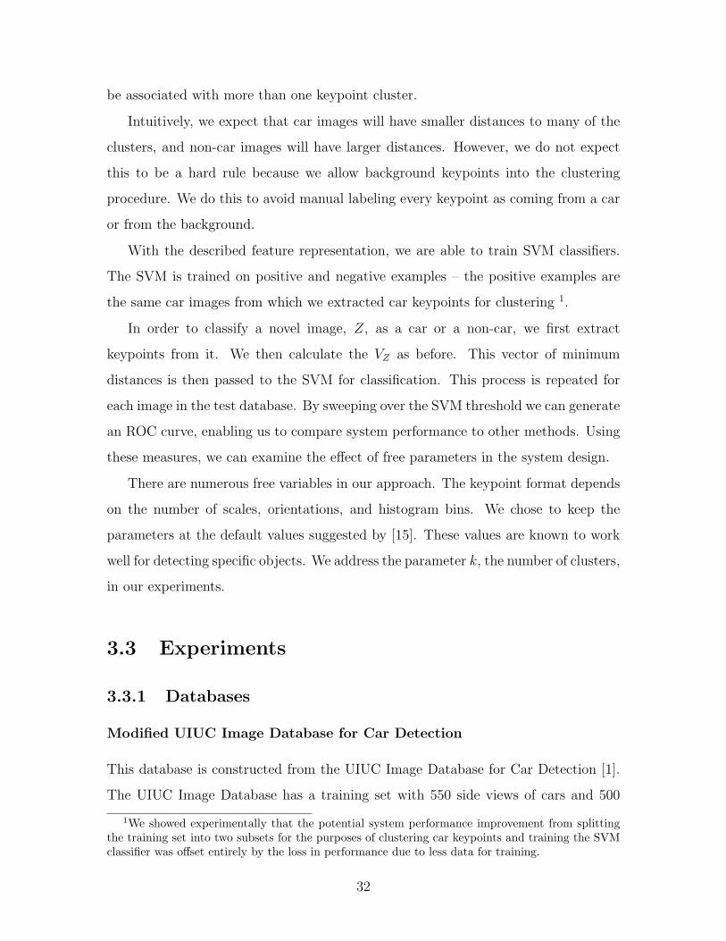
3-2 Examples of cars and non-cars from the training and test set in the

StreetScenes Subset Database. . . . . . . . . . . . . . . . . . . . . . . 33

3-3 Difficult car examples from the StreetScenes Subset database. . . . . 34

3-4 ROC plot comparing performance on the UIUC Image Database of

SVM classifiers using various common feature spaces. . . . . . . . . . 35

3-5 ROC plot comparing performance on the StreetScenes Subset Database

of SVM classifiers using various common feature spaces. . . . . . . . . 36

3-6 Error rates on the UIUC Database positive and negative test sets. 170

positive examples, 4183 negative examples in test set. . . . . . . . . . 37

3-7 Comparison of the Keypoint-based Car Detector to Global SVM Clas-

sifiers on the UIUC Image Database. . . . . . . . . . . . . . . . . . . 38

3-8 Comparison of the Keypoint-based Car Detector to Global SVM Clas-

sifiers on the StreetScenes Subset Database. . . . . . . . . . . . . . . 38

3-9 Performance on the UIUC Image Database of the Keypoint-based Car

Detector as we vary k, the number of cluster centroids used. . . . . . 39

9

3-10 Performance on the StreetScenes Subset Database of the Keypoint-

based Car Detector as we vary k, the number of cluster centroids used. 40

3-11 Positive training images from the UIUC database displaying the most

expressive keypoints. The size of the keypoint represents the scale at

which the keypoint was taken. A keypoint is displayed in red if it is

a ’car keypoint’. A keypoint is colored green if it is a ’background

keypoint’. . . . . . . . . . . . . . . . . . . . . . . . . . . . . . . . . . 40

3-12 Comparison of the SIFT Descriptor with a Local Patch Descriptor for

the keypoint-based car detector. The experiment was performed on

the UIUC Image Database. . . . . . . . . . . . . . . . . . . . . . . . . 41

4-1 Examples of patches used as templates and their associated binary

spatial mask indicating the region over which a feature is extracted.

These regions are chosen to be a square of size 5x5 pixels. The size of

the patches range from 3x3 pixels to 14x14 pixels. . . . . . . . . . . . 44

4-2 Examples of part detections for wheels and the sidepanel. A threshold

is chosen by setting the number of permissible false detections to one

false positive for every 106 windows. . . . . . . . . . . . . . . . . . . . 47

4-3 Labelings of car images in the Street Scenes Labeled Subset. . . . . . 50

4-4 ROC curves from 4 component classifiers: wheels, roof, sidepanel,

windshield. The components are in order with the curve for wheels

in the upper left corner and the curve for the windshield in the lower

right corner. . . . . . . . . . . . . . . . . . . . . . . . . . . . . . . . . 51

10

4-5 ROC curve comparing performance of three different component com-

bination schemes. The worst performance is the system that just uses

the maximum value of each component. The next worse curve is the

ROC curve for the method that concatenates the maximum value of

detection and the position of the maximum detection for each part

into one feature vector. The curves on top use the maximum-value-in-

subregion approach for varying number of subregions. ROC curves are

generated from a dataset of cropped cars and non-cars. . . . . . . . . 52

4-6 ROC curves comparing system performance on a test set between our

component-based system (solid line) and the baseline global car detec-

tor (dashed line). . . . . . . . . . . . . . . . . . . . . . . . . . . . . . 53

4-7 Correct Detections . . . . . . . . . . . . . . . . . . . . . . . . . . . . 54

4-8 Difficult examples of cars that were detected correctly. The left side

image has a truck with many wheels that was correctly detected. The

right has pictures of the front and back views of cars. These views are

not represented well by the three components used in the component

detection system. Specifically, the wheels and the sidepanel do not

show up in these cars. . . . . . . . . . . . . . . . . . . . . . . . . . . 54

4-9 False Detections: found in trees, on walls, on the windshield of a car,

and parts of a store front. . . . . . . . . . . . . . . . . . . . . . . . . 55

4-10 Interesting Examples of Incorrect Detections: grouping multiple cars

together, a bridge between two cars in a row, off-center detection due

to occlusion, multiple partitioned detections for one object. . . . . . . 56

11

12

Chapter 1

Introduction

Our day-to-day lives are abound with instances of object detection. Crossing the

street after first checking for cars, recognizing a familiar face, identifying sushi, and

finding Waldo in those childhood “Where’s Waldo?” picture books are all examples of

object detection. We as humans are surprisingly good at it. Unfortunately, building

a system that can perform object detection reliably is a dauntingly complicated and

difficult computational task. When compared to existing computer vision systems,

each one of us can more accurately and more quickly identify instances from many

more different classes of objects. More importantly, we can more quickly learn to

identify new instances of objects, and new classes of objects. Although a great deal

of research has already been performed to advance the field and improve the capability

and robustness of object detection systems, we are still many years from closing the

performance gap between the human visual system and engineered object detection

systems.

The difficulty in object detection is compounded by the high variability in ap-

pearance between objects of the same class and the additional variability between

instances of the same object due to differences in viewing conditions. Specifically, an

object detection system must be able to detect the presence or absence of an object,

such as a car, under different illuminations, scales, poses, and under differing amounts

of background clutter.

13

1.1 Problem Statement

Recent studies in object detection have shown that a component-based approach

is more resilient to partial occlusions of objects, and more robust to natural pose

variations, than the traditional holistic approach. These component-based object

detectors are built hierarchically, where simpler detectors first locate components of

an object, and a combination classifier makes the final detection with the outputs from

each of the component detectors as features. Accurate results have been reported in

both face [11, 12, 3] and pedestrian detection [18, 17]. In this thesis, we apply a

component-based approach to a more difficult domain: cars in natural images of

street scenes. We demonstrate reasonable results for two different component-based

systems, despite the large inherent variability of cars in these scenes.

Detecting cars is a considerably more difficult problem than detecting faces or

pedestrians. The human face has a simple, semi-rigid structure, where the localization

of face components does not vary much between samples. Cars have a semi-rigid

structure as well, but that structure will vary more between samples, because their

shapes and configurations have been designed with product differentiation in mind.

Besides the intra-class variations due to color, shape, and ornamentation, which

similarly plague face and pedestrian detection systems (to a lesser degree), there are

other issues that complicate car detection. First, we wish to be able to detect a car

irrespective of the view or the out-of-plane rotation. Compared to the other object

classes, the car also has more views that are interesting. One major difficulty in object

detection is the fact that different views of the same object can look very different,

because an image is essentially the projection of a 3D object onto a 2D plane. The

face has far fewer degrees of freedom, because only frontal views, side profiles, and

any pose in between are of general interest. This restriction reduces the intra-instance

variability due to viewing conditions. Usually different classifiers are trained for the

different views as was done in [24] to achieve rotation invariance.

Second, the car has many more candidates for components, and only a subset of

these components are viewable from any particular perspective. For example, the

14

tail lights would typically be obscured if the headlights are in plain view and the

license plates are usually not viewable from a direct side view. In a component-based

detection framework, this suggests that we ought to place more emphasis on the

component detection combination algorithm. This situation can be compared to face

or pedestrian detection with large amounts of occlusion.

In this thesis, we explore the selection of object-specific components, the learning

of the selected components, and the combination of component detections in order to

determine whether or not there is an advantage in building hierarchical classifiers for

a broad set of object classes. We expect that this framework works well for classes

where an object is comprised of distinct identifiable components or parts and they

are arranged in a limited set of well-defined geometric configurations. Although our

ultimate goal is generic object class detection, we hope to gain more intuition on the

object class detection problem by concentrating on the classification and detection of

cars. Our incremental one-object-at-a-time approach toward achieving a “dictionary”

of object detectors may also aid researchers in building application-specific object

detectors.

1.2 Motivation

Object detection and recognition are necessary components in an artificially-intelligent

autonomous system. They provide such systems a context that facilitates interaction

with its outside environment. Eventually we expect these artificially-intelligent au-

tonomous systems to venture onto the streets of our world, thus requiring detection

of objects commonly found on the street. From a systems-perspective, the low-level

recognition of objects provides a layer of abstraction to the system, allowing it to

perform scene-understanding by manipulating the objects that were detected rather

than using the underlying pixel intensities. The need to develop extensible object de-

tection frameworks for reliable detection of many different kinds of objects in natural

scenes increases as such autonomous systems become more prevalent.

Aside from the noble pursuit of artificial intelligence, object recognition has seen

15

an increase in commercial interest. Academic research has been successfully applied

in the areas of law enforcement, surveillance, authentication and access control sys-

tems, and computer chip verification processes to name a few. The human face, in

particular, has received much attention because of its prominence in visual images

and the multitude of emergent applications. The task of identifying generic objects

in still images can also greatly enhance the computing experience of the Internet and

the World Wide Web. For example, object detection can be applied to labeling and

indexing images found on the web, allowing users to manipulate the medium with

more sophistication. As the number of real-world applications of object recognition

increase, there is a need for accurate recognition systems that can be easily applied to

different object classes with fewer constraints on extrinsic imaging parameters, such

as pose, illumination, scale, position, etc.

Our long-term goal is toward a system that can accurately locate in an image

particular instances from many generic object class. Such a system can serve as a

“dictionary of classifiers”, usable as a primitive for scene-understanding applications.

Success can ultimately be measured by comparing the system’s accuracy to that of a

human performing the same task.

The direct motivation and an immediate application of the work in this thesis is

to facilitate the tedious and error-prone labeling of objects in a database of natural

images of street scenes, a database that we can use to study reliable object detection

for scene-understanding applications. For this reason, we stress extensibility in terms

of applicability to many object classes over the raw accuracy for each individual

object class. The database contains images of objects in the ’wild’. This makes

the task of object detection even more difficult, as objects may be in any natural

pose, illumination, scale, position, etc. Our systems are designed with these multiple

degrees of variation in mind.

16

1.3 Outline of Thesis

Chapter 2 discusses the background required to realize an object detection system.

We discuss the object (binary) classifier in a statistical learning framework, survey

and evaluate a set of feature spaces, and finally develop the framework in which the

classifier is applied to candidate patches in an image. Where relevant we discuss

previous work in the field.

In Chapter 3, we present an hierarchical car classifier that outperforms holistic

car classifiers in distinguishing between a car patch and a non-car patch. This car

classifier combines measures of similarity to diagnostic keypoints, which are local

features around points extracted by an interest operator. We then evaluate this

system and compare it to holistic classifiers. Finally in Chapter 4, we demonstrate

a working system that combines component detections for the car detection task.

The components we used were chosen a priori and examples in the database were

hand-labeled.

We conclude the thesis in Chapter 5 and discuss future avenues of research in

Chapter 6.

17

18

Chapter 2

Object Detection

Object detection in an image, the act of finding an instance of an object class in

an image, can be viewed as the application of pattern recognition. We first build

a classifier that can distinguish between an image patch that belongs to the target

object class and one that does not belong to the target object class. We primarily

employ Support Vector Machines (SVMs) for classification, but our component-based

system in Chapter 4 employs an AdaBoost classifier for the component detections.

These classifiers are discussed in Section 2.1.

After we build object classifiers, we search through all windows of the image at

various scales, to identify patches belonging to the target object class. We discuss this

aspect of object detection in Section 2.2. Outside this chapter, we use the term object

detection for both the classification of a particular window and the task of searching

all such windows with a classifier.

From a systems perspective, it is advantageous to view the object detection task

as the application of an object classifier to many windows of an image at different

scales. This view essentially decouples the task of building good classifiers from the

infrastructure required to actually perform the detection. As suggested in [2], we

ought to use the best classifier possible and the best infrastructure.

19

2.1 Object Classifier

Classifying whether an image patch belongs to a particular object class or not is a

pattern recognition task. Specifically, if we are given a feature vector representing an

image or a transformation on the image, we would like to be able to classify whether

or not the image belongs to the particular object class. As phrased, it becomes a

statistical learning problem, where we learn from example images of objects how to

distinguish between objects that belong to the target object class and objects that

do not belong to the target object class. We learn the discriminative features that

separate the two classes, so that when we are given new images, we can determine

whether or not it belongs to the target class with a certain level of confidence.

In this framework, there are two choices open to design. The first is the choice of

classifier to use. There are many choices that have been shown to work reasonably

well, like neural networks, SVMs, and variants of the AdaBoost algorithm to name a

few. The second choice is the choice of feature space. Successful systems have been

developed using the original gray-scale pixel intensities, gradient images, edge maps,

wavelet coefficients, and many others.

In the statistical learning literature, there has been much debate over the choice of

classification algorithms. In most cases, it is the choice of features that is important

for accurate results. A carefully chosen classification algorithm will give marginal

improvements. In the following sections, we give a brief overview of the classifiers

used in this paper without much fanfare about its choice. Afterward, we will provide

an empirical comparison of different feature spaces for the car classification task in

question.

2.1.1 Statistical Learning Framework

Learning is the problem of deriving a predictive function that when given a new

observation x can assign the correct label y to the observation with some level of

confidence. The function is judged by its ability to generalize to new unseen examples.

Supervised learning uses a large training set of examples, a set of (x, y) pairs to derive

20

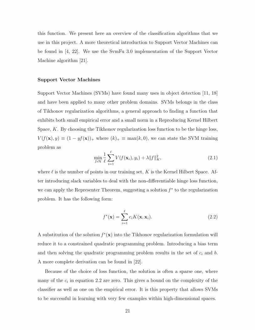
this function. We present here an overview of the classification algorithms that we

use in this project. A more theoretical introduction to Support Vector Machines can

be found in [4, 22]. We use the SvmFu 3.0 implementation of the Support Vector

Machine algorithm [21].

Support Vector Machines

Support Vector Machines (SVMs) have found many uses in object detection [11, 18]

and have been applied to many other problem domains. SVMs belongs in the class

of Tikhonov regularization algorithms, a general approach to finding a function that

exhibits both small empirical error and a small norm in a Reproducing Kernel Hilbert

Space, K. By choosing the Tikhonov regularization loss function to be the hinge loss,

V (f (x), y) ≡ (1 − yf (x))+ where (k)+ ≡ max(k, 0), we can state the SVM training

problem as

minf εH

1

`

∑i=1

V (f (xi), yi) + λ‖f ‖2K , (2.1)

where ` is the number of points in our training set, K is the Kernel Hilbert Space. Af-

ter introducing slack variables to deal with the non-differentiable hinge loss function,

we can apply the Representer Theorem, suggesting a solution f ∗ to the regularization

problem. It has the following form:

f ∗(x) =∑i=1

ciK(x,xi). (2.2)

A substitution of the solution f ∗(x) into the Tikhonov regularization formulation will

reduce it to a constrained quadratic programming problem. Introducing a bias term

and then solving the quadratic programming problem results in the set of ci and b.

A more complete derivation can be found in [22].

Because of the choice of loss function, the solution is often a sparse one, where

many of the ci in equation 2.2 are zero. This gives a bound on the complexity of the

classifier as well as one on the empirical error. It is this property that allows SVMs

to be successful in learning with very few examples within high-dimensional spaces.

21

In this thesis, we primarily use an SVM formulation with a linear dot product

kernel. With a linear kernel, the solution of equation 2.2 reduces to

f ∗(x) = w · x, (2.3)

where w is normal vector that specifies the separating hyperplane. We take the sign

of the solution in equation 2.3 to be the classification. There are a few considerations

that need to be taken care of when a separating hyperplane cannot be found in the

feature space. This is primarily related to the choice of C in the SVM formulation.

C is the parameter that controls the trade-off between classification accuracy and the

norm of the function.

Note that we are specifically concerned with binary SVM classification, however

there exist methods to combine binary SVM classifiers for the purpose of multiclass

classification. See [23] for an empirical comparison of the many schemes. Additionally,

SVMs can be formulated to handle regression problems.

Boosting Algorithm for Classification

Boosting algorithms have been applied successfully in numerous object detection sys-

tems [34, 30]. In [34], an object detection framework is built to process images rapidly

and with high detection rates. They apply AdaBoost [26] to build an attentional cas-

cade of progressively more refined classifiers.

A boosting algorithm additively combines the outputs of weak learners into a

strong learner. A strong learner is a classifier that can learn the underlying target

function arbitrarily well, given enough training data, while a weak learner is one that

can barely perform better than chance, given enough data. AdaBoost is an iterative

procedure to construct a strong classifier from several weak classifiers. A typical weak

classifier to use is a simple decision or regression stump of the form

h(x) = aδ(xi > θ) + b, (2.4)

22

where xi is the ith component of the feature vector x, θ is a threshold, δ is an indicator

function, and a and b are regression parameters to best fit the data. The final classifier

is a linear combination of the weak classifiers of the form:

H(x) =M∑i=1

hi(x), (2.5)

where M is the number of rounds of boosting.

An AdaBoost algorithm typically works as follows. We first start off weighting

each training data example equally. For each round of boosting, we fit a weak classifier

to the weighted data. Then we adaptively adjust the weights on the training data

for the next round of boosting to place more emphasis on errors made in the current

round. There are a few variants of this algorithm; the differences lie in how the

algorithm computes the re-weighting of the training data [8]. In this thesis, we use

the Gentle AdaBoost variant described in [8]. It has been shown to work well in

object detection applications [30, 14]. AdaBoost has also been found to be resilient

to overfitting of data.

2.1.2 Feature Spaces

As mentioned before, a main task of object detection is determining the feature space

in which to learn. Various feature spaces have been successfully employed for the

tasks of face and pedestrian detection. From experience, it seems that the choice of

feature space is heavily dependent on the object class. A feature space that works

best for faces may not work well for pedestrians, and vice versa.

For face detection, a comparison of gray-scale pixel values, first derivative of gray-

scale images, and wavelets is available in [11]; it suggests that gray-scale pixel values

are often a good enough choice. On the other hand, haar wavelet coefficients were

found to work well in pedestrian detection [17, 18].

In Section 3.3.2, we perform our own comparison of various feature spaces for the

task of classifying cropped images of cars and non-cars. On one dataset, we found

that gray-scale pixels and a histogram of edge orientations works well in distinguishing

23

between cars and non-cars. On a different data set, the histogram of edge orientations

did not perform well at all. From this study, it seems that gray-scale pixels are also

a good enough choice for the class of cars.

[11, 29] also evaluate methods of feature reduction like Principle Component Anal-

ysis (PCA) and feature selection based on an ordering of the coefficients of the re-

sulting SVM hyperplane specified by w. Other feature selection methods like the one

proposed in [36] can also be used.

2.1.3 Global Approaches

Many early face detection systems like that of [19] and [24, 32] employed a holistic

approach to the problem of face detection. These approaches take the face as a single

unit and perform classification on features generated from the entire face. In these

systems, SVMs or neural networks were trained to discriminate between face and non-

face images. Rotation invariance was built into the system in [24] by training several

neural networks, one for each possible discretized amount of rotation. In [20, 24],

improvements were made by using virtual examples to increase the size of the training

set. Virtual examples were generated by rotating, translating, or scaling the original

faces. Including these virtual examples reduces the sensitivity of the classifier to these

variations, which may be present in new test examples. Confusable non-faces have

also been bootstrapped into the training set to improve the accuracy of the classifiers.

2.1.4 Component-based Approaches

Recently, component-based approaches to object detection like the ones in [18, 12,

3, 37] have become more fashionable. The intuitive motivation behind a component-

based approach is that each part of an object should be less sensitive to changes

in illumination, pose, and rotation than the object as a whole. Component-based

systems can also be engineered to deal with partial occlusion by clutter or strong

directional lighting. Furthermore, they can leverage the geometric information and

constraints in the configurations of the components. Empirically, they have been

24

shown to produce better accuracy than global, holistic approaches [3].

A typical component-based object detection architecture involves selecting compo-

nents to be trained, selecting a feature description for each component, and combining

detected components for the final object classification. In selecting the components

to be trained, systems like [11] use the typical facial features, such as eyes, the nose,

and the mouth. The system has then been improved in [12] to select salient features

automatically using a region-growing algorithm with a statistical bound. In [35, 6], in-

terest operators were employed to select keypoints in images, and a generative model

is learned on a selected subset of these keypoints to explain the data. Besides the

choice of components, systems differ in their choice of feature description. Gray-scale

pixel value features can be used like in [3]. The system in [28] extracts features from

the wavelet decomposition of images to build a histogram-based classifier.

Once part examples have been detected in an image, component-based object

detection systems will employ a second-layer classifier to determine whether or not

the parts taken as a whole belong to a member of the object class or not. Several

approaches can be taken. Some approaches perform a likelihood ratio test that deter-

mines whether a given configuration of detected parts is more likely to have stemmed

from a member of the object class or not [3, 6]. Others like [37] search in a set of pre-

viously seen configurations for the best geometrically consistent subset of extracted

parts from the image. In [12], an SVM is trained to decide whether or not the set of

positions and confidences of each part is likely to have come from a face. This SVM

is then evaluated on the features from the best detections for each component.

2.2 Object Detection Framework

The final step of object detection in images is to apply the learned classifier to all the

potential windows of the image at different scales. Objects are considered detected

in a window if the classifier has a high enough activation value. In [1], they the coin

the term classifier activation map for the outputs of the classifier on windows of the

image.

25

Objects in images may appear at different scales depending on the depth of the

object with respect to the camera. Therefore it is important to search the image at

different scales in order to detect all objects. To keep the number of features of the

classifier fixed, we iteratively scale the image by a specified amount.

In object detection, the choice that impacts the visible results of detection most

is the threshold at which the classifier operates. Usually, our classifiers are too per-

missive in what they classify as members of the target object class. This is because

our training set does not reflect well the actual probability distribution of objects,

over-stressing the presence of positive instances of the target class. We alleviate this

by choosing an operating point on a Receiver Operator Characteristic (ROC) plot

in the region of low false positives. We choose an operating point that satisfies our

requirements against false positives; it is usually a choice based on the number of

inspected windows.

Another important issue to resolve is the multiple detections that may occur for

the same object. These multiple detections may also occur across a few scales. In

many respects all these detections are correct, but a single detection is often required

for some applications. A few methods have been employed to reduce the multiplicity

of correct detections. The most common method partitions the detected windows

into disjoint, non-overlapping groups, and the best (highest activating) detection in

each group is used. Problems arise here when we have multiple cars very close to

each other and the non-overlapping constraint may be too strong. Another approach

is to take, as the best location, the maximum activation in a specified neighborhood

of potential locations across multiple scales. If two locally maximal activations occur

in close proximity to each other but are outside of each others neighborhood, then

both activations are considered detections.

2.3 Miscellaneous

In computer vision, a natural extension of object detection is to the task of object

identification, where an instance of a particular object is classified into one of many

26

smaller subclass. In particular for faces, it is often useful to determine the identity

of the face wherever a face has been detected. Although we do not address the

identification aspect of recognition in this paper, we can very easily generalize binary

classifiers for multiclass classification in order to perform such object identification. In

general, one-versus-all has been shown to work well for many multiclass classification

tasks [23].

27

28

Chapter 3

Hierarchical Car Classifier using an

Interest Operator

In the previous chapter, we discussed a few systems suggesting that accurate and

powerful object detectors can be built in a hierarchical component-based fashion. In

this chapter, we plan to demonstrate that this hierarchical structure is advantageous

for object detection in images with cars. We discuss a hierarchical car classifier based

on salient features extracted by an interest operator. The classifier operates by first

locating keypoints in the test image with an interest operator. These keypoints are

then compared against a corpus of car-specific keypoints learned from the training

data. The resulting similarity vector is input into an SVM classifier. We then compare

the performance of this classifier to non-hierarchical classifiers. In this chapter, we

view the keypoints in our corpus of car-specific keypoints as components of cars. The

technical and philosophical validity of this claim is open to debate. Nevertheless, we

are able to show that this hierarchical “component-based” approach indeed works

well for cars.

29

3.1 Interest Operator and SIFT Feature Descrip-

tor

Extracting distinctive and invariant features quickly from images is an important task

for a hierarchical object detection system. It was decided early in the development of

this system to use the interest operator discussed in [15] to make this process rapid

and robust. Other options were to use those operators described in [7, 9]. The Lowe

Interest Operator detects interesting points or keypoints by locating extrema in

D(x, y, σ) = (G(x, y, kσ)−G(x, y, σ)) ∗ I(x, y), (3.1)

where I(x,y) is the input image, and G(x, y, σ) is the variable scale gaussian,

G(x, y, σ) =1

2πσ2exp−(x2+y2)/2σ2

. (3.2)

Each interest point is parameterized by not only the x, y, and scale, but also a dom-

inant orientation computed from the neighborhood of D(x, y, σ). These parameters

impose a 2D coordinate system, providing invariance to translation, scale, and rota-

tion [16].

At each keypoint we record the Scale Invariant Feature Transform (SIFT) of the

image. The SIFT feature descriptor is designed to be invariant to changes in illu-

mination and changes due to 3D viewpoint. These invariances address issues that

often plague object detection systems. The computation of the descriptor involves

first computing the gradient image of magnitudes and orientations and then dividing

a local region around the keypoint into 4x4 sample regions. An orientation histogram

with 8 orientation bins is created for each of the regions, where each gradient image

pixel contributes its gradient magnitude into the histogram entry (keyed by the gra-

dient orientation). Care is taken to avoid boundary effects and effects due to small

changes in keypoint location. A threshold is used to limit the contribution of large

gradient magnitudes in each histogram entry. This step coupled with renormalization

30

is performed to reduce the effects of illumination changes. The final result is a 128

dimensional feature vector shown to work very well for object detection tasks. Details

are available in [16].

It has been shown empirically [15, 5] that this combination of keypoint detector

and image feature works well for object detection.

3.2 Keypoint-based Car Detector

Our goal is to construct a hierarchical car detector by automatically learning car-

specific features and then learning a combination classifier. We chose to center our

features on the keypoint detections returned by the algorithm described in [15], be-

cause they are robust, computationally efficient, and invariant to a number of common

image transforms. We take the following approach. First we extract keypoints from

car images in our training set. Each keypoint is a 128-dimensional vector representing

a 4x4 array of orientation histograms with 8 bins in each histogram. These keypoints

may come from an actual car or from the background in a car training image. We

cluster the keypoints into a fixed number, k, of clusters, using k-means clustering. Let

this set of cluster centroids be the set K, and let Kj denote the jth cluster centroid.

Our initial hope was that these clusters would represent semantic car parts. The next

step in training a classifier is representing the training data in terms of the expression

strength of these parts.

In order to train an SVM classifier, we must be able to convert the image, I, from

the training set into a fixed-length feature vector, VI . Let T be the set of keypoints

extracted from image I. The vector VI has elements VI(j), j ∈ [1, . . . , k], such that

VI(j) = minr∈T

‖Kj − r‖ (3.3)

Our fixed-length feature vector is now a k-dimensional vector of distances between

clusters from the training data and keypoints from the image. In general, since there

may be more clusters than there are keypoints in an image, a particular keypoint may

31

be associated with more than one keypoint cluster.

Intuitively, we expect that car images will have smaller distances to many of the

clusters, and non-car images will have larger distances. However, we do not expect

this to be a hard rule because we allow background keypoints into the clustering

procedure. We do this to avoid manual labeling every keypoint as coming from a car

or from the background.

With the described feature representation, we are able to train SVM classifiers.

The SVM is trained on positive and negative examples – the positive examples are

the same car images from which we extracted car keypoints for clustering 1.

In order to classify a novel image, Z, as a car or a non-car, we first extract

keypoints from it. We then calculate the VZ as before. This vector of minimum

distances is then passed to the SVM for classification. This process is repeated for

each image in the test database. By sweeping over the SVM threshold we can generate

an ROC curve, enabling us to compare system performance to other methods. Using

these measures, we can examine the effect of free parameters in the system design.

There are numerous free variables in our approach. The keypoint format depends

on the number of scales, orientations, and histogram bins. We chose to keep the

parameters at the default values suggested by [15]. These values are known to work

well for detecting specific objects. We address the parameter k, the number of clusters,

in our experiments.

3.3 Experiments

3.3.1 Databases

Modified UIUC Image Database for Car Detection

This database is constructed from the UIUC Image Database for Car Detection [1].

The UIUC Image Database has a training set with 550 side views of cars and 500

1We showed experimentally that the potential system performance improvement from splittingthe training set into two subsets for the purposes of clustering car keypoints and training the SVMclassifier was offset entirely by the loss in performance due to less data for training.

32

Figure 3-1: Examples of cars and non-cars from the training and test set in theModified UIUC Image Database for Car Detection. All car images are side viewsof cars where the car is spatially localized in the image. The first and third row areexamples of positive and negative training images. The second row contains the cropsfrom the test images of the UIUC Image Database; these images were used as ourpositive test images. The last row contains examples of negative test images.

Figure 3-2: Examples of cars and non-cars from the training and test set in theStreetScenes Subset Database.

non-car images. Each of these gray scale images are 40× 100. The cars are roughly

of the same build and at the same position, and are subject to possible occlusion and

differences in illumination. We used this training set unmodified. The provided test

set contains cars to be located in images with a large amount of background. For our

purposes, we cropped out the first car from each of the test images to serve as our

positive test set and provided our own set of negative examples. In total, we have

170 side views of cars and 4183 non-cars for the test set. See Figure 3-1 for examples

of cars and non-cars in the training and test set.

33

Figure 3-3: Difficult car examples from the StreetScenes Subset database.

StreetScenes Subset Database

The StreetScenes database contains high resolution (up to 768× 1024) images of cars

in a natural environment. The database contains cars, trucks, and buses in many

poses, different degrees of occlusion, as well as variations in illumination. In order to

simplify the problem, we have decided to concentrate on side views of cars. We have

performed semi-automated sorting of the cars in the database by pose in order to

extract the side views of cars. We also extract non-cars from the StreetScenes images

with a similar distribution in sizes. All images are converted into gray scale, extracted

at a fixed aspect ratio, and finally scaled down to a fixed image size. Figure 3-2 shows

examples of images from this database. Our training database contains 350 images

of cars and 4000 images of non-cars. The test database contains 149 images of cars

and 4059 images of non-cars.

Car detection on the StreetScenes database is a considerably more difficult task

than on the UIUC Image Database. Because the side views of cars were semi-

automatically extracted to improve the generality of our methods, errors did occur

as shown in Figure 3-3. Also, the StreetScenes Subset database contains images of

bulldozers and buses, making the classification task difficult.

3.3.2 Global (Non-hierarchical) SVM Classifiers - A survey

of feature spaces

For comparison purposes, we perform the learning task on these databases using

canonical statistical learning machines, vis. SVM and k-Nearest Neighbor technique.

34

Figure 3-4: ROC plot comparing performance on the UIUC Image Database of SVMclassifiers using various common feature spaces.

We explored system performance using various common feature spaces and a few

novel ones. ROC curves comparing results of different global (non-hierarchical) SVM

classifiers are provided in Figures 3-4 and 3-5. All the ROC plots concentrate in

the low false positive region, because this is the region believed to be important

for the application of car detection in images. All generalizations made in the low

false positive region extends to the high false positive region unless otherwise stated.

Table 3-6 gives error rates comparing SVM performance to k-Nearest Neighbors for

the UIUC Image Database.

The first feature space we explored was the original gray pixel intensities. We

applied the following pre-processing steps. First, each gray scale image is scaled down

to a common size. We vary this to measure the effect on performance. Histogram

equalization is then performed on each image individually to remove variations in

image brightness and contrast.

In [31, 12], it was found that by using Principle Component Analysis (PCA) the

dimensionality of the data could be reduced, while preserving system performance, or

possibly even improving it. Along with gray scale features, we tested PCA features

in this stage of the experiment. We tried running the experiment with 5, 10, 20, and

40 principle components.

35

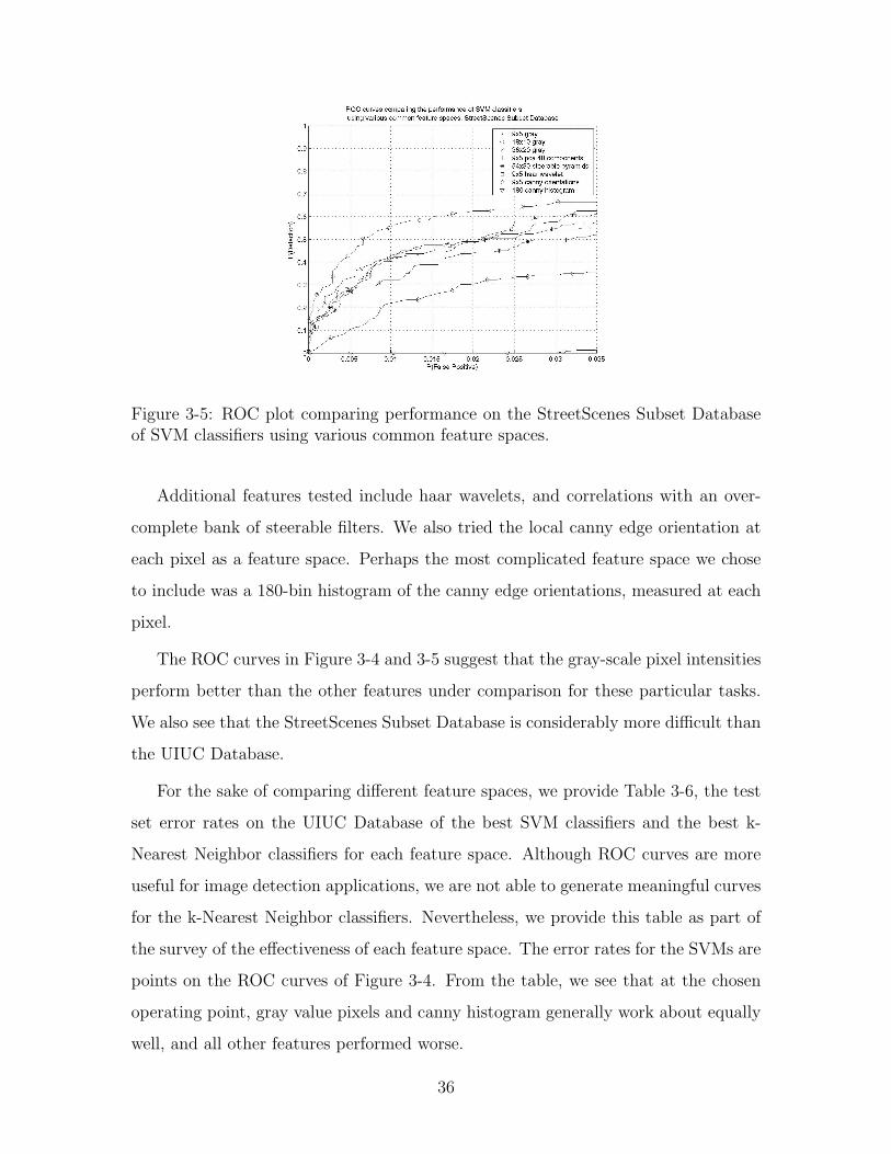
Figure 3-5: ROC plot comparing performance on the StreetScenes Subset Databaseof SVM classifiers using various common feature spaces.

Additional features tested include haar wavelets, and correlations with an over-

complete bank of steerable filters. We also tried the local canny edge orientation at

each pixel as a feature space. Perhaps the most complicated feature space we chose

to include was a 180-bin histogram of the canny edge orientations, measured at each

pixel.

The ROC curves in Figure 3-4 and 3-5 suggest that the gray-scale pixel intensities

perform better than the other features under comparison for these particular tasks.

We also see that the StreetScenes Subset Database is considerably more difficult than

the UIUC Database.

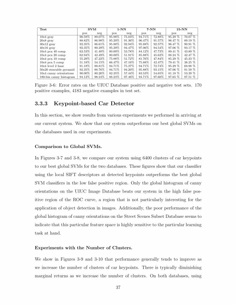
For the sake of comparing different feature spaces, we provide Table 3-6, the test

set error rates on the UIUC Database of the best SVM classifiers and the best k-

Nearest Neighbor classifiers for each feature space. Although ROC curves are more

useful for image detection applications, we are not able to generate meaningful curves

for the k-Nearest Neighbor classifiers. Nevertheless, we provide this table as part of

the survey of the effectiveness of each feature space. The error rates for the SVMs are

points on the ROC curves of Figure 3-4. From the table, we see that at the chosen

operating point, gray value pixels and canny histogram generally work about equally

well, and all other features performed worse.

36

Test SVM 1-NN 7-NN 15-NNpos neg pos neg pos neg pos neg

10x4 gray 90.59% 89.07% 95.88% 75.03% 94.71% 72.88% 95.29 % 70.07 %20x8 gray 88.82% 86.98% 95.29% 91.36% 96.47% 91.57% 96.47 % 89.19 %30x12 gray 92.35% 86.61% 95.88% 92.94% 95.88% 92.57% 96.47 % 90.91 %40x16 gray 92.35% 90.29% 95.29% 94.47% 97.06% 94.54% 97.06 % 93.17 %10x4 pca 40 comp 63.53% 41.40% 80.00% 53.78% 84.12% 47.73% 89.41 % 43.89 %10x4 pca 20 comp 62.94% 42.49% 80.00% 51.91% 85.88% 45.62% 88.24 % 42.47 %10x4 pca 10 comp 55.29% 47.22% 75.88% 51.72% 81.76% 47.84% 85.29 % 45.33 %10x4 pca 5 comp 51.18% 54.15% 66.47% 47.16% 75.88% 42.47% 79.41 % 38.25 %10x4 level 2 haar 91.18% 88.81% 94.71% 75.37% 94.71% 72.74% 95.29 % 69.98 %50x20 steerable pyramid 92.35% 88.76% 94.71% 94.20% 95.88% 93.15% 97.06 % 91.59 %10x4 canny orientations 90.00% 80.26% 82.35% 57.44% 83.53% 54.65% 81.18 % 53.39 %180-bin canny histogram 94.12% 98.24% 88.24% 97.46% 94.71% 97.60% 97.65 % 97.51 %

Figure 3-6: Error rates on the UIUC Database positive and negative test sets. 170positive examples, 4183 negative examples in test set.

3.3.3 Keypoint-based Car Detector

In this section, we show results from various experiments we performed in arriving at

our current system. We show that our system outperforms our best global SVMs on

the databases used in our experiments.

Comparison to Global SVMs.

In Figures 3-7 and 3-8, we compare our system using 6400 clusters of car keypoints

to our best global SVMs for the two databases. These figures show that our classifier

using the local SIFT descriptors at detected keypoints outperforms the best global

SVM classifiers in the low false positive region. Only the global histogram of canny

orientations on the UIUC Image Database beats our system in the high false pos-

itive region of the ROC curve, a region that is not particularly interesting for the

application of object detection in images. Additionally, the poor performance of the

global histogram of canny orientations on the Street Scenes Subset Database seems to

indicate that this particular feature space is highly sensitive to the particular learning

task at hand.

Experiments with the Number of Clusters.

We show in Figures 3-9 and 3-10 that performance generally tends to improve as

we increase the number of clusters of car keypoints. There is typically diminishing

marginal returns as we increase the number of clusters. On both databases, using

37

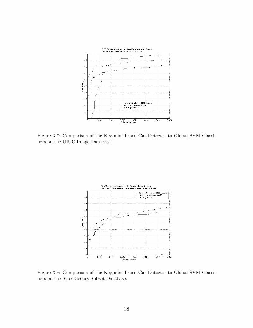
Figure 3-7: Comparison of the Keypoint-based Car Detector to Global SVM Classi-fiers on the UIUC Image Database.

Figure 3-8: Comparison of the Keypoint-based Car Detector to Global SVM Classi-fiers on the StreetScenes Subset Database.

38

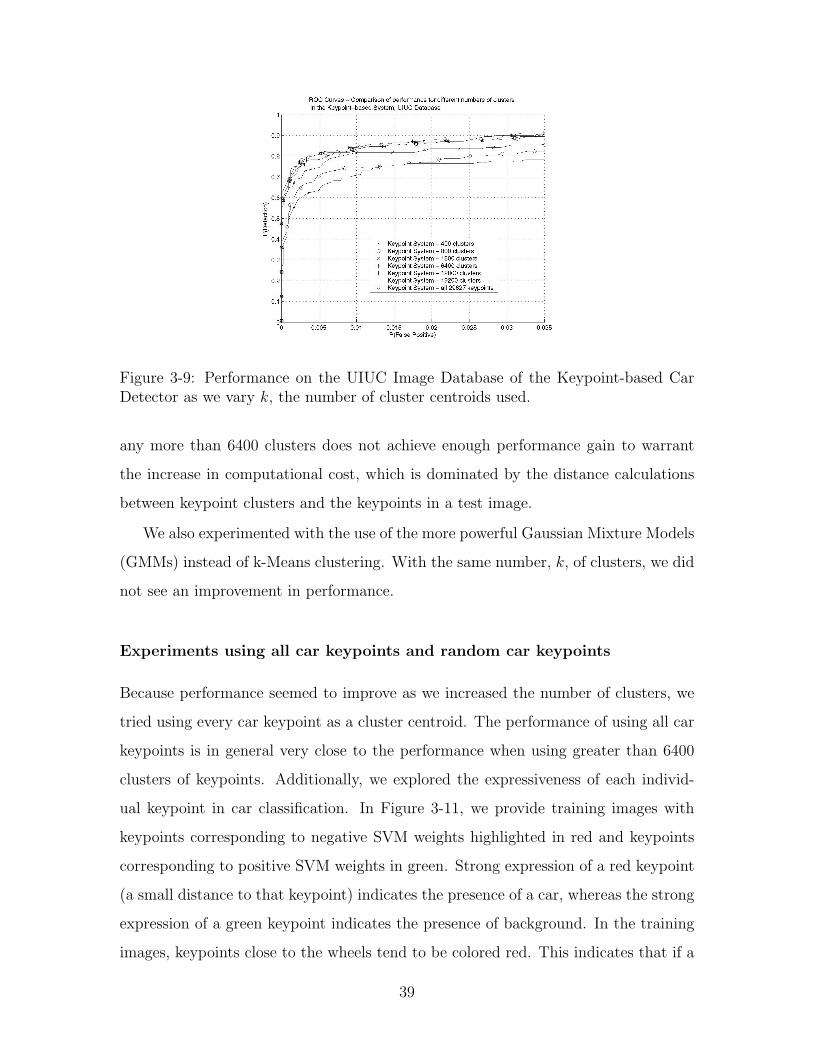
Figure 3-9: Performance on the UIUC Image Database of the Keypoint-based CarDetector as we vary k, the number of cluster centroids used.

any more than 6400 clusters does not achieve enough performance gain to warrant

the increase in computational cost, which is dominated by the distance calculations

between keypoint clusters and the keypoints in a test image.

We also experimented with the use of the more powerful Gaussian Mixture Models

(GMMs) instead of k-Means clustering. With the same number, k, of clusters, we did

not see an improvement in performance.

Experiments using all car keypoints and random car keypoints

Because performance seemed to improve as we increased the number of clusters, we

tried using every car keypoint as a cluster centroid. The performance of using all car

keypoints is in general very close to the performance when using greater than 6400

clusters of keypoints. Additionally, we explored the expressiveness of each individ-

ual keypoint in car classification. In Figure 3-11, we provide training images with

keypoints corresponding to negative SVM weights highlighted in red and keypoints

corresponding to positive SVM weights in green. Strong expression of a red keypoint

(a small distance to that keypoint) indicates the presence of a car, whereas the strong

expression of a green keypoint indicates the presence of background. In the training

images, keypoints close to the wheels tend to be colored red. This indicates that if a

39

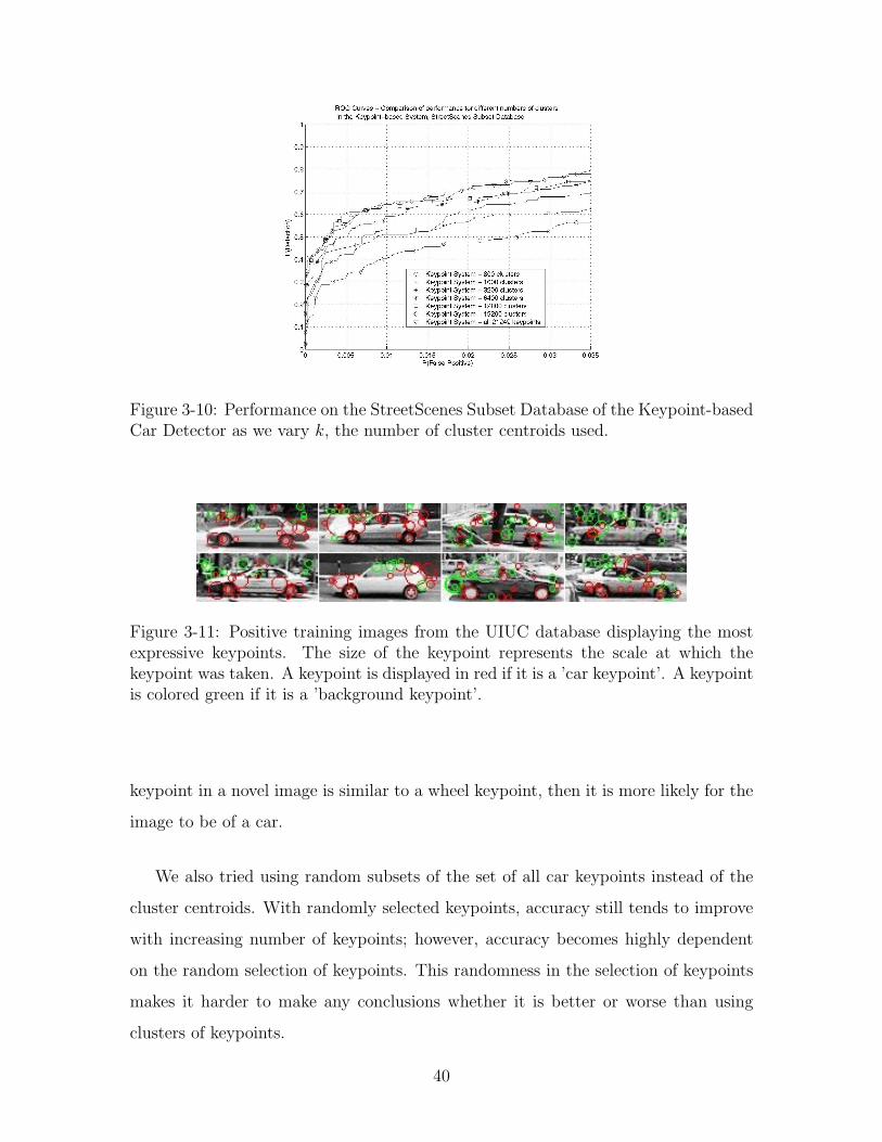
Figure 3-10: Performance on the StreetScenes Subset Database of the Keypoint-basedCar Detector as we vary k, the number of cluster centroids used.

Figure 3-11: Positive training images from the UIUC database displaying the mostexpressive keypoints. The size of the keypoint represents the scale at which thekeypoint was taken. A keypoint is displayed in red if it is a ’car keypoint’. A keypointis colored green if it is a ’background keypoint’.

keypoint in a novel image is similar to a wheel keypoint, then it is more likely for the

image to be of a car.

We also tried using random subsets of the set of all car keypoints instead of the

cluster centroids. With randomly selected keypoints, accuracy still tends to improve

with increasing number of keypoints; however, accuracy becomes highly dependent

on the random selection of keypoints. This randomness in the selection of keypoints

makes it harder to make any conclusions whether it is better or worse than using

clusters of keypoints.

40

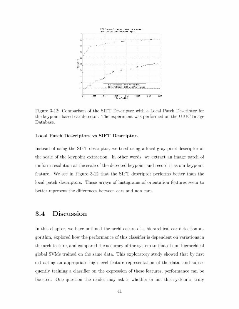
Figure 3-12: Comparison of the SIFT Descriptor with a Local Patch Descriptor forthe keypoint-based car detector. The experiment was performed on the UIUC ImageDatabase.

Local Patch Descriptors vs SIFT Descriptor.

Instead of using the SIFT descriptor, we tried using a local gray pixel descriptor at

the scale of the keypoint extraction. In other words, we extract an image patch of

uniform resolution at the scale of the detected keypoint and record it as our keypoint

feature. We see in Figure 3-12 that the SIFT descriptor performs better than the

local patch descriptors. These arrays of histograms of orientation features seem to

better represent the differences between cars and non-cars.

3.4 Discussion

In this chapter, we have outlined the architecture of a hierarchical car detection al-

gorithm, explored how the performance of this classifier is dependent on variations in

the architecture, and compared the accuracy of the system to that of non-hierarchical

global SVMs trained on the same data. This exploratory study showed that by first

extracting an appropriate high-level feature representation of the data, and subse-

quently training a classifier on the expression of these features, performance can be

boosted. One question the reader may ask is whether or not this system is truly

41

a part-based car detector. For certain the SIFT features learned from the data are

diagnostic for cars, as evidenced by the gain in performance over SVMs trained on

other reasonable features. Also the SIFT features are spatially constrained; data from

the image is only inspected at or near the keypoint returned by the interest operator.

While the clusters we extract in the k-means step represent spatially constrained car

specific features, they do not necessarily correspond to what a human would consider

as a semantic car part 2.

While the performance of our system is better than that of the best global (non-

hierarchical) SVM technique we implemented, it is also considerably more complicated

in structure. One might ask if the additional performance is worth the cost. What

we have seen empirically is that: while a simple SVM and our technique might do

equally well at detecting a car that is very similar to the majority of the training

database, our method has the advantage when abnormal conditions, such as a partial

occlusion or a strong lighting condition, cause part of the car to look dissimilar to

what is expected.

One unexpected result in the course of this experiment was that in general it is

better to use as many clusters as possible, almost all the way out to the extreme where

every keypoint from the training database is itself its own cluster. In this way our

system bears some similarity to a fragmented nearest neighbor technique. Whereas

in nearest neighbor classification a test image is compared via a distance metric to

every car and non car image in the training data, in our technique every interesting

car point is compared to every keypoint from the training data.

In implementing this system, we did not utilize geometrical constraints as is usu-

ally done when building a component-based detection system. Early experiments have

shown that including the location does indeed provide additional improvements, but

further work must be done to investigate the best way to incorporate this information

into the system.

2Some clusters regularly locate the wheel of the car, in this case we would consider the cluster tobe a semantic car part

42

Chapter 4

Component-based Approach

In this chapter, we present a component-based object detection system using pre-

selected and manually labeled components. The system is very similar in design to

other component-based systems in face and pedestrian detection [12, 18]. For the

component detectors, we choose to use the features proposed by [30]. These features

were chosen for their computational efficiency and ease of implementation. The full

system architecture is discussed in the next section with experiments and conclusions

to follow.

4.1 System Architecture

We propose a two-tiered system, where we first detect car parts and then combine

these component detections to make the final car detection. We choose car parts that

we believe are salient. These parts include: wheels, headlights, taillights, the roof, the

back bumper, rear view mirrors, the windshield, and the “sidepanel”, a rectangular

region between the wheels that includes the shadow underneath the car and lower

half of the car doors. Classifiers are learned for each of these parts as described in

Section 4.1.1. In Section 4.1.2, we discuss how the part detections are used to train

a top-layer car classifier.

43

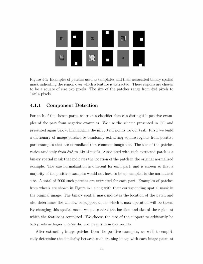
Figure 4-1: Examples of patches used as templates and their associated binary spatialmask indicating the region over which a feature is extracted. These regions are chosento be a square of size 5x5 pixels. The size of the patches range from 3x3 pixels to14x14 pixels.

4.1.1 Component Detection

For each of the chosen parts, we train a classifier that can distinguish positive exam-

ples of the part from negative examples. We use the scheme presented in [30] and

presented again below, highlighting the important points for our task. First, we build

a dictionary of image patches by randomly extracting square regions from positive

part examples that are normalized to a common image size. The size of the patches

varies randomly from 3x3 to 14x14 pixels. Associated with each extracted patch is a

binary spatial mask that indicates the location of the patch in the original normalized

example. The size normalization is different for each part, and is chosen so that a

majority of the positive examples would not have to be up-sampled to the normalized

size. A total of 2000 such patches are extracted for each part. Examples of patches

from wheels are shown in Figure 4-1 along with their corresponding spatial mask in

the original image. The binary spatial mask indicates the location of the patch and

also determines the window or support under which a max operation will be taken.

By changing this spatial mask, we can control the location and size of the region at

which the feature is computed. We choose the size of the support to arbitrarily be

5x5 pixels as larger choices did not give us desirable results.

After extracting image patches from the positive examples, we wish to empiri-

cally determine the similarity between each training image with each image patch at

44

the location where the patch was originally extracted. This is a form of template

matching and is very similar in spirit to the distance vector that we compute in the

interest operator inspired system described in Chapter 3. The training procedure is

as follows. For each positive and negative part image in our training set (already

rescaled to a common image size), we compute a 2000 dimensional feature vector,

one feature for each extracted patch. Each element of the vector is the maximum of

the normalized correlation between the training image and an image patch under the

patch’s corresponding spatial mask. In more mathematical terms, for every patch i,

we compute the feature

vi = maxx∈Sw{|Iσ ⊗ gf |}, (4.1)

where Sw is the support of the spatial mask wi, ⊗ represents normalized correlation

between the rescaled example image Iσ and the extracted patch gf . σ is the scale of the

original image. These features have been found to be good for template matching [33].

After extracting these features from hundreds of positive training examples and

negative training examples, we train a Gentle AdaBoost classifier, selecting the 100

most diagnostic image patch features out of the set of 2000. We use simple regression

stumps for the weak classifiers as described in Section 2.1.1. We chose to use 100

features, because the system in [30] performs reasonably well with only 70 independent

features for various object classes. In that paper, they advocate the sharing of features

between object classes. We do not share features in our system, but it is an option

we may find useful to explore.

We now test on a novel image using our part classifiers. To do so, we apply

each classifier over all possible windows and at multiple scales. In order to speed up

computation, we approximate the calculation of vi in Equation 4.1 as

vi = (wi ∗ |Iσ ⊗ gf |p)1/p, (4.2)

where ∗ is the convolution operation and p is chosen to be a large value (we choose p

= 101). According to [30], setting p > 10 allows Equation 4.2 to approximate Equa-

tion 4.1. Setting p = 1 gives us features that are average filter responses. Increasing

45

the value of p allows us to vary from generating features that provide a representative

global description of the patch to features that are very well localized [30]. We have

chosen a single high value of p in this system, but concede that this choice may differ

for each part classifier.

An additional benefit of the approximation for the maximum of the normalized

correlation under the spatial mask stems from the linearity of the operations. This

enables us to work with the whole test image rather than windows of the test image.

In other words, let Iσ be the whole image rather than a window of the image, where

σ is the scale at which the entire image is rescaled.

Each convolution with the spatial mask can be efficiently computed using the inte-

gral image trick [34]. We now address the computation of the normalized correlation.

In [30], the computational cost of convolving an image patch with a whole image

is reduced by approximating the patch with a combination of linearly separable 1D

filters. We do not use this decomposition, but we do propose a variant to the normal-

ized cross correlation that is typically used. Instead of normalizing the correlation

by the product of the standard deviation of the template and the standard deviation

of the region under the template in the original image, we normalize by the product

of the average of the template and the average of the region under the template.

Both normalized correlation and our variant work as part detectors, but our variant

is faster to compute. An additional benefit is that these features are always positive.

Part detection on a test image is then performed by first extracting features using

equation 4.2 for each feature utilized by the Gentle AdaBoost classifier. This results

in images of normalized correlation values, which are then passed through the corre-

sponding weak classifier regression stumps. These output values are then summed up

to form the strong classifier outputs, the final detection values. We can view these

final detection values as a result image, where highly illuminated regions represent

strong detections of the part. The next step of car part combination will take these

part detections as input. Applying the procedures described in Section 2.2 allows us

to identify unique part detections. We provide examples of such detections for wheels

and the sidepanel in Figure 4-2. We do not perform suppression of multiple compo-

46

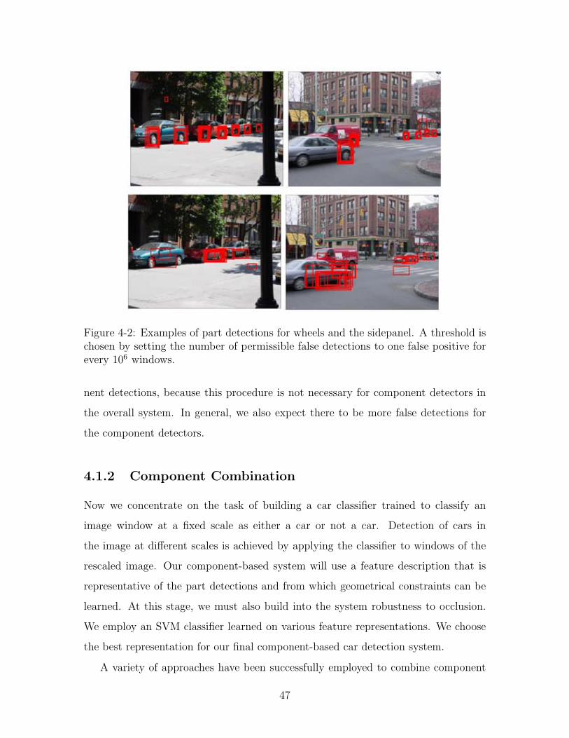
Figure 4-2: Examples of part detections for wheels and the sidepanel. A threshold ischosen by setting the number of permissible false detections to one false positive forevery 106 windows.

nent detections, because this procedure is not necessary for component detectors in

the overall system. In general, we also expect there to be more false detections for

the component detectors.

4.1.2 Component Combination

Now we concentrate on the task of building a car classifier trained to classify an

image window at a fixed scale as either a car or not a car. Detection of cars in

the image at different scales is achieved by applying the classifier to windows of the

rescaled image. Our component-based system will use a feature description that is

representative of the part detections and from which geometrical constraints can be

learned. At this stage, we must also build into the system robustness to occlusion.

We employ an SVM classifier learned on various feature representations. We choose

the best representation for our final component-based car detection system.

A variety of approaches have been successfully employed to combine component

47

detectors. In [18], the largest detection value in a pre-specified region for each

component is used as a feature vector. An SVM is trained using these features,

thereby learning the variability in component detection values for the class of cars.

The geometrical information is embedded in the constrained search for the maximum

detection value. Robustness to occlusion is learned by the SVM, given enough rep-

resentative examples. We cannot employ this approach effectively because a priori

it is difficult to constrain the locations of our components to pre-specified regions in

a common image plane. Another approach, taken in [12], is to additionally pass the

location of the maximum detection in the image plane. A final (and the most success-

ful) approach divides the image plane into a finite number of regions and records the

maximum part detection value in each region. The maximum value in each region for

each component is the feature representation from which an SVM is learned. This

approach also embeds geometrical information in the features. The calculation of the

max in many subwindows can be performed more efficiently by taking advantage of

the integral image trick and a formulation similar to Equation 4.2. We present results

comparing these methods of component combination in Section 4.2.

4.1.3 Car Detection

After learning the combination classifier, we can classify an image window of fixed size

as either a car or a non-car with some confidence. We then apply this classifier to all

possible windows of an image over multiple scales, and record the classifier outputs.

Given these outputs, we apply techniques similar to the ones presented in Section 2.2

in order to set a threshold for the classifier and remove multiple detections of a single

object. These classifier outputs will also allow us to measure the performance of our

system.

As described in Section 2.2, we must now set an operating threshold for the car

detector, and then develop a scheme to suppress multiple detections. The threshold

is chosen to satisfy a requirement on the number of allowable false detections. This

is very application-specific and we choose a threshold corresponding to a point on

the ROC curve. Typically, selecting the threshold corresponding to one false positive

48

for every 106 inspected windows is sufficient. We suppress multiple detections of a

single object by iteratively accepting detections that do not overlap too much with

previously accepted detections. The detections are sorted by detection strength be-

forehand and we do not allow any overlap of more than 25% with previously accepted

detections. This method provides good visual results and is simple to implement.

4.2 Experiments

4.2.1 Database

We use a different subset of the StreetScenes subset than was presented in Sec-

tion 3.3.1. We did not use the same database because we did not want to concentrate

only on the side views of cars. From this subset, we manually labeled the parts of the

cars from a total of 158 images. The parts that were labeled are wheels, headlights,

taillights, roof, back bumper, rear view mirrors, windshield and the sidepanel. Fig-

ure 4-3 shows the labelings of two cars. The labeling process associates a bounding

polygon (potentially not convex) to each car part in the image. A lot of effort was

spent to ensure a complete and consistent labeling of each part. Unfortunately, this

manual process can be error prone. One apparent flaw in the labelings is that the

bounding rectangle may include some clutter from the surrounding background. This

is because we did not implement a zoom-in mechanism to get a tight bound polygon

on the part. Another difficulty occurred because we did not manually associate each

labeled part with the car it belongs to. With a few heuristics, we were able to re-

establish most of these associations, but the process is not free of error. We decided

to work with this noisy data and hope for the best.

We split the labeled images into a training and a test set. 111 images were used

for the training set and 47 images were left for the test set. We also included a total

of 337 images without component labels into the test set. For any classifier that we

train, the training set was taken only from training set images and the test set was

taken only from test set images. For example, we only use the 256 positive car images

49

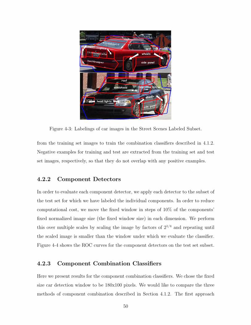
Figure 4-3: Labelings of car images in the Street Scenes Labeled Subset.

from the training set images to train the combination classifiers described in 4.1.2.

Negative examples for training and test are extracted from the training set and test

set images, respectively, so that they do not overlap with any positive examples.

4.2.2 Component Detectors

In order to evaluate each component detector, we apply each detector to the subset of

the test set for which we have labeled the individual components. In order to reduce

computational cost, we move the fixed window in steps of 10% of the components’

fixed normalized image size (the fixed window size) in each dimension. We perform

this over multiple scales by scaling the image by factors of 21/4 and repeating until

the scaled image is smaller than the window under which we evaluate the classifier.

Figure 4-4 shows the ROC curves for the component detectors on the test set subset.

4.2.3 Component Combination Classifiers

Here we present results for the component combination classifiers. We chose the fixed

size car detection window to be 180x100 pixels. We would like to compare the three

methods of component combination described in Section 4.1.2. The first approach

50

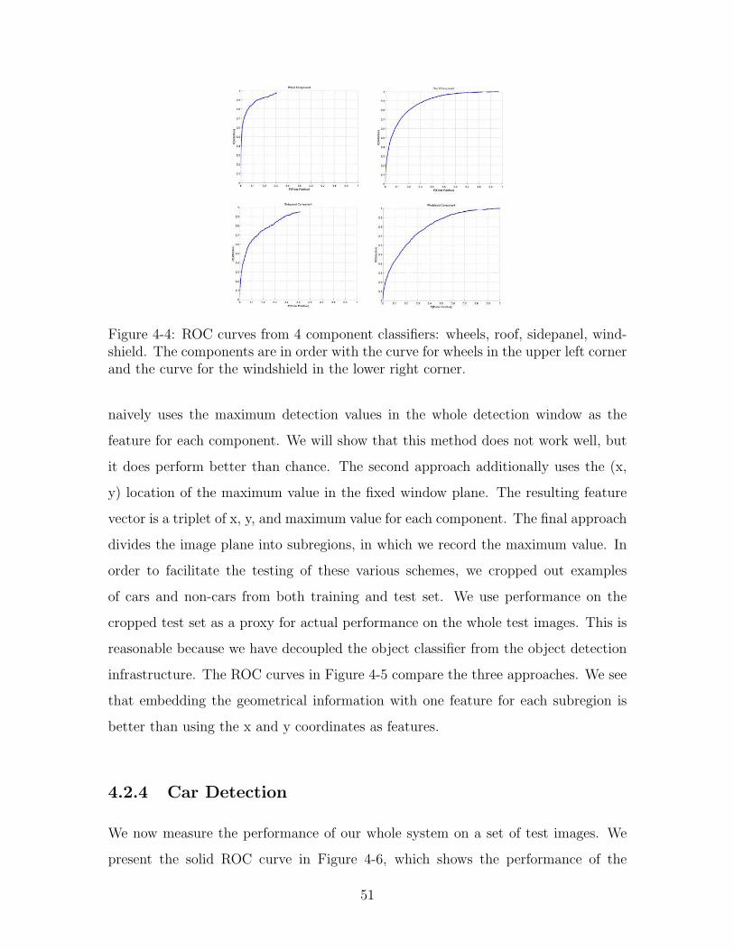
Figure 4-4: ROC curves from 4 component classifiers: wheels, roof, sidepanel, wind-shield. The components are in order with the curve for wheels in the upper left cornerand the curve for the windshield in the lower right corner.

naively uses the maximum detection values in the whole detection window as the

feature for each component. We will show that this method does not work well, but

it does perform better than chance. The second approach additionally uses the (x,

y) location of the maximum value in the fixed window plane. The resulting feature

vector is a triplet of x, y, and maximum value for each component. The final approach

divides the image plane into subregions, in which we record the maximum value. In

order to facilitate the testing of these various schemes, we cropped out examples

of cars and non-cars from both training and test set. We use performance on the

cropped test set as a proxy for actual performance on the whole test images. This is

reasonable because we have decoupled the object classifier from the object detection

infrastructure. The ROC curves in Figure 4-5 compare the three approaches. We see

that embedding the geometrical information with one feature for each subregion is

better than using the x and y coordinates as features.

4.2.4 Car Detection

We now measure the performance of our whole system on a set of test images. We

present the solid ROC curve in Figure 4-6, which shows the performance of the

51

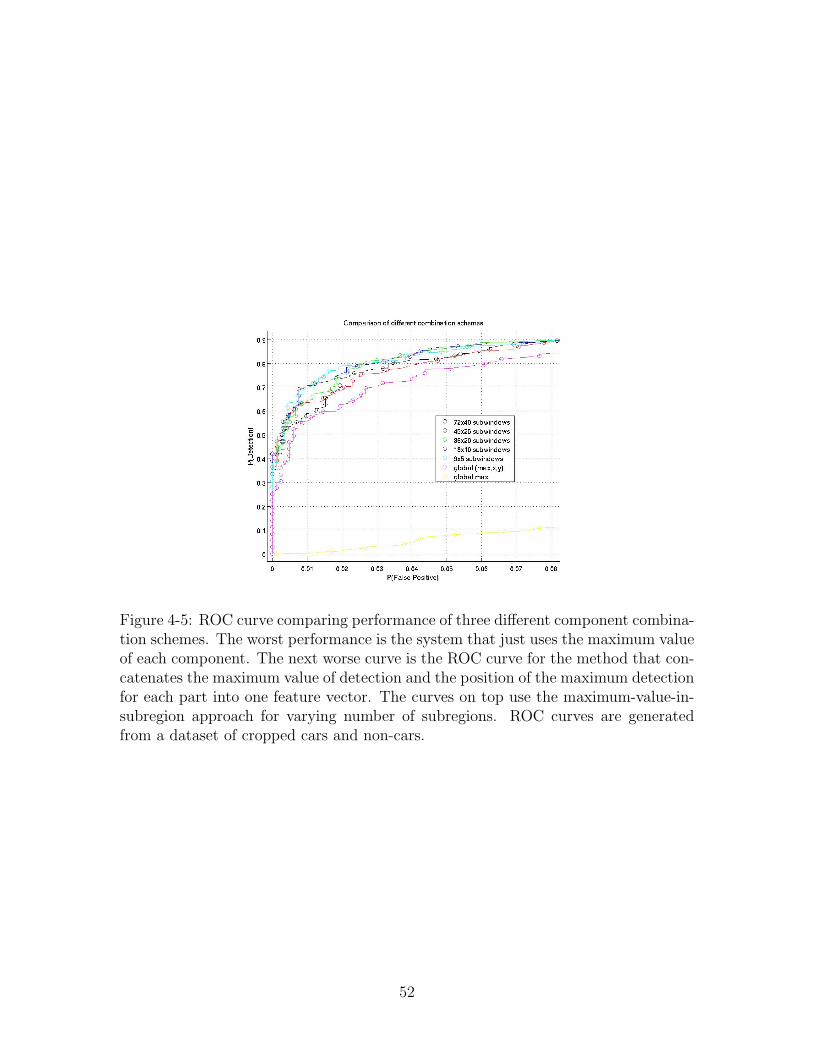
Figure 4-5: ROC curve comparing performance of three different component combina-tion schemes. The worst performance is the system that just uses the maximum valueof each component. The next worse curve is the ROC curve for the method that con-catenates the maximum value of detection and the position of the maximum detectionfor each part into one feature vector. The curves on top use the maximum-value-in-subregion approach for varying number of subregions. ROC curves are generatedfrom a dataset of cropped cars and non-cars.

52

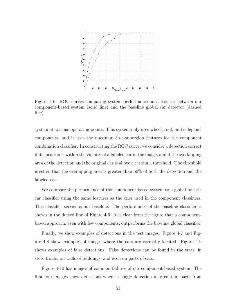
Figure 4-6: ROC curves comparing system performance on a test set between ourcomponent-based system (solid line) and the baseline global car detector (dashedline).

system at various operating points. This system only uses wheel, roof, and sidepanel

components, and it uses the maximum-in-a-subregion features for the component

combination classifier. In constructing the ROC curve, we consider a detection correct

if its location is within the vicinity of a labeled car in the image, and if the overlapping

area of the detection and the original car is above a certain a threshold. The threshold

is set so that the overlapping area is greater than 50% of both the detection and the

labeled car.

We compare the performance of this component-based system to a global holistic

car classifier using the same features as the ones used in the component classifiers.

This classifier serves as our baseline. The performance of the baseline classifier is

shown in the dotted line of Figure 4-6. It is clear from the figure that a component-

based approach, even with few components, outperforms the baseline global classifier.

Finally, we show examples of detections in the test images. Figure 4-7 and Fig-

ure 4-8 show examples of images where the cars are correctly located. Figure 4-9

shows examples of false detections. False detections can be found in the trees, in

store fronts, on walls of buildings, and even on parts of cars.

Figure 4-10 has images of common failures of our component-based system. The

first four images show detections where a single detection may contain parts from

53

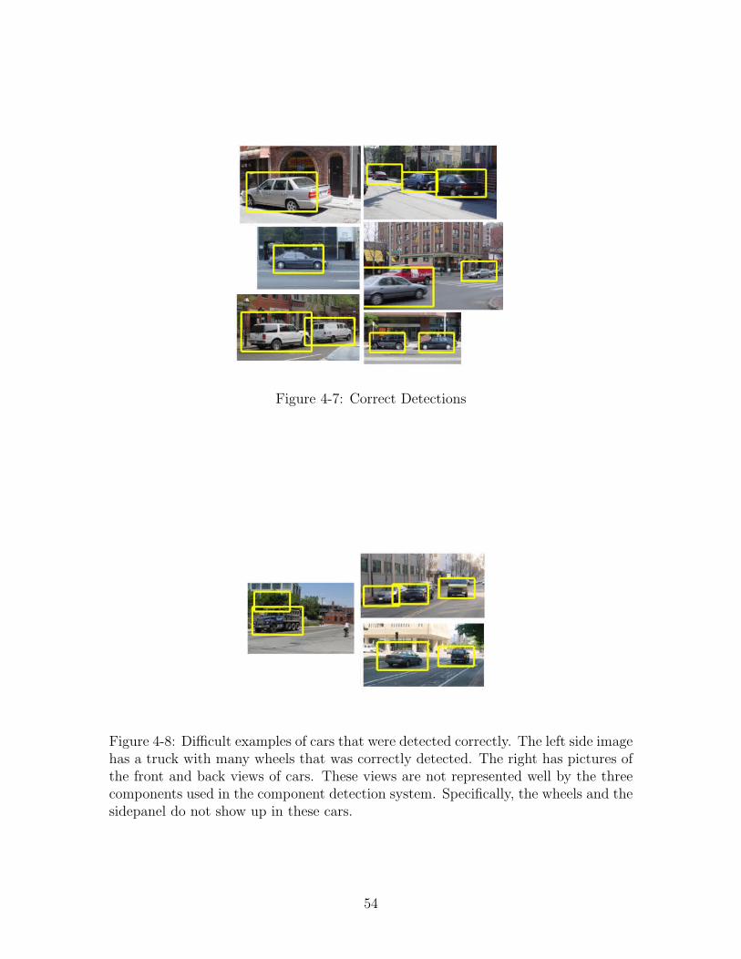
Figure 4-7: Correct Detections

Figure 4-8: Difficult examples of cars that were detected correctly. The left side imagehas a truck with many wheels that was correctly detected. The right has pictures ofthe front and back views of cars. These views are not represented well by the threecomponents used in the component detection system. Specifically, the wheels and thesidepanel do not show up in these cars.

54

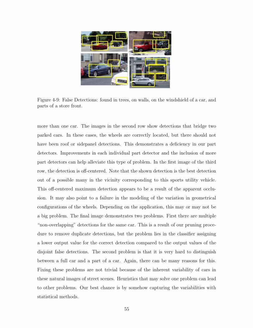
Figure 4-9: False Detections: found in trees, on walls, on the windshield of a car, andparts of a store front.

more than one car. The images in the second row show detections that bridge two

parked cars. In these cases, the wheels are correctly located, but there should not

have been roof or sidepanel detections. This demonstrates a deficiency in our part

detectors. Improvements in each individual part detector and the inclusion of more

part detectors can help alleviate this type of problem. In the first image of the third

row, the detection is off-centered. Note that the shown detection is the best detection

out of a possible many in the vicinity corresponding to this sports utility vehicle.

This off-centered maximum detection appears to be a result of the apparent occlu-

sion. It may also point to a failure in the modeling of the variation in geometrical

configurations of the wheels. Depending on the application, this may or may not be

a big problem. The final image demonstrates two problems. First there are multiple

“non-overlapping” detections for the same car. This is a result of our pruning proce-

dure to remove duplicate detections, but the problem lies in the classifier assigning

a lower output value for the correct detection compared to the output values of the

disjoint false detections. The second problem is that it is very hard to distinguish

between a full car and a part of a car. Again, there can be many reasons for this.

Fixing these problems are not trivial because of the inherent variability of cars in

these natural images of street scenes. Heuristics that may solve one problem can lead

to other problems. Our best chance is by somehow capturing the variabilities with

statistical methods.

55

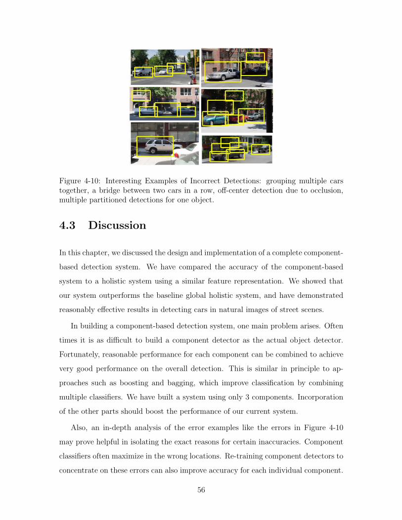
Figure 4-10: Interesting Examples of Incorrect Detections: grouping multiple carstogether, a bridge between two cars in a row, off-center detection due to occlusion,multiple partitioned detections for one object.

4.3 Discussion

In this chapter, we discussed the design and implementation of a complete component-

based detection system. We have compared the accuracy of the component-based

system to a holistic system using a similar feature representation. We showed that

our system outperforms the baseline global holistic system, and have demonstrated

reasonably effective results in detecting cars in natural images of street scenes.

In building a component-based detection system, one main problem arises. Often

times it is as difficult to build a component detector as the actual object detector.

Fortunately, reasonable performance for each component can be combined to achieve

very good performance on the overall detection. This is similar in principle to ap-

proaches such as boosting and bagging, which improve classification by combining

multiple classifiers. We have built a system using only 3 components. Incorporation

of the other parts should boost the performance of our current system.

Also, an in-depth analysis of the error examples like the errors in Figure 4-10

may prove helpful in isolating the exact reasons for certain inaccuracies. Component

classifiers often maximize in the wrong locations. Re-training component detectors to

concentrate on these errors can also improve accuracy for each individual component.

56

We may also be able to harness contextual information shared between component

detections like the pairwise position statistics method used in [3]. Methods like these

can clean up our noisy detections and thus remove unnecessary variations seen by our

learning algorithms.

The reader may also question our choices for parts of the car. These parts were

chosen a priori in order to parallelize research. We are very much interested in

building component-based systems where the components are automatically chosen,

systems like the ones in [1, 12]. The system as described is independent of the

component choices, so automatically chosen components are easily incorporated into

the system design. We hope to be able to automatically select parts that are both

semantic and diagnostic for car detection.

57

58

Chapter 5

Conclusion

In Chapter 3, we presented a car classification scheme based on learning similarities

to features extracted by an interest operator. We then showed that this hierarchi-

cal system holds its own when compared to traditional global holistic approaches

using SVMs. Although it is debatable whether or not the clusters of car-specific

keypoints used in the system can be considered car parts, they do allow us to build

hierarchical two-layered car classifiers. In Chapter 4, we presented the design and im-

plementation of a complete system to locate cars in images based on the detections of

human-specified components. We showed reasonable results for detections on a very

difficult data set of natural images of street scenes. We provide a comparison with a

holistic system using the same features, showing the advantage of a component-based

approach.

The construction of these viable component-based systems with hierarchical struc-

tures seems to indicate an advantage for component-based approaches compared to

traditional holistic approaches, for a broad class of objects. We have seen empirically

that component-based systems are more robust against abnormal conditions, such as

partial occlusion from clutter and strong lighting. Although there is strong evidence

that accuracy can be improved, component-based systems are considerably more com-

plicated in structure, requiring more computational resources. Various optimizations

have been designed into our systems, and possibly more can be realized.

Although we were able to demonstrate the capabilities of a component-based

59

system for the class of cars in natural images of street scenes, it is still an open

question as to whether or not a component approach can generalize to object classes

such as buildings or trees where components are not easily defined and potential

components do not occur in semi-fixed locations.

5.1 Comparison with Prior Work in Car Detection

For completeness, we describe a few other car detection systems and discuss the

differences between their work and ours. We first begin by comparing our own two

systems. We have gone from one extreme where parts are determined by an interest

operator to another extreme where parts are specified by humans. There is also

a disparity in the number of of components used. Whereas we have pre-defined the

number of components for the system in Chapter 4, the system in Chapter 3 performs

well when we have chosen many example components from our training data, to the

point where each component stemmed from a particular car example. In this way,

we prefer to have a set number of components, because it allows us to more directly

control the complexity of our classifier. A formal comparison of the two systems

would be interesting, but has not yet been performed.

In [27], a car detection system is designed to be able to detect cars over a variety

of views. Their approach is not component-based, but can be considered hierarchical.

They learn different classifiers that specialize on different views of a car, and a car is

detected if any of the classifiers activated above a threshold. For each of these classi-

fiers, they perform a likelihood ratio test after modeling the conditional probabilities

of each class with products of histograms. This system has been shown to work well

on a test set. We would like to perform a fair comparison of our systems to their

system as a benchmark, however, we do not have access to their training data.

In [1], a component-based hierarchical car detector is developed. A vocabulary of

parts are extracted using an interest operator similar to what was done in Chapter 3.

They learn a Sparse Network of Winnows (SNoW) classifier on features that represent

the image by its parts and observed spatial relations. They observe good accuracy

60

on a heavily-constrained data set of side views of fixed size cars. In Chapter 3, we

used a cropped version of their dataset for our own experiments, but did not perform

a direct comparison with the work performed in [1]. However, a comparison has been

made between the SNoW car classifier and a linear SVM classifier in [2] showing that

it performs about as well as a global linear SVM.

61

62

Chapter 6

Future Work

In this section, we describe some immediate work for improving the systems as de-

scribed in this thesis. We also advertise philosophies and future work to be done at

the Center for Biological and Computational Learning (CBCL).

6.1 Derivative Work

As is the case with any engineered system, many design choices can potentially be

tweaked for overall system improvements. To our best efforts, we have put forth

our choices of parameters and the design decisions for our implementation. Many of

these selections can be varied; unfortunately, there are too many possibilities to fully

explore in a limited amount of time.

In Chapter 3, we describe a system for classification using interest operators, but

we did not investigate the use of the interest operator to identify regions of interest

in order to reduce the computational complexity in scanning all windows of an image

over many scales. This is a very interesting area of research with lots of potential for

improving object detection. [25] describes a system that uses an interest operator to

identify regions where an object may be found. Harnessing these ideas can potentially

improve both the accuracy and the running time of our algorithms. Additionally, the

procedure for applying the hierarchical car classifier is prohibitively computationally

expensive. It may be fruitful to investigate other clustering techniques in order to

63

decrease the number of training keypoints used in the feature representation.

In Chapter 4, we investigated one feature representation using the normalized

correlation under the spatial mask. We used Gentle AdaBoost classifiers for the

component detectors. We first attempted to use SVM classifiers with gray-scale pixel

values as features, however, the running time became burdensome when dealing with

such large images as the ones in the StreetScenes database. This strained our ability

to fully research the capabilities of this system, and we are hesitant to make any

claims as to which feature representation and classifier pair is better for the task.

We essentially took the first approach that worked well and ran with it. We hope to

return to address the many questions that remain unanswered.

A general problem in building a component-based system is that the building the

component detectors is often just as hard as building the actual detector. Fortunately,

we have found that we can achieve good car detection despite subpar component

detection. More work is required to improve each component detector and providing

detectors for more components.

6.2 More Objects

In order to realize our goal of a “dictionary” of classifiers, we must work on more

objects. We advocate a one-object-at-a-time iterative procedure towards this goal.

We also stress the importance of extensible methods that work over a large class

of objects rather than dwelling on a single object. The experience in building each

object class detector may potentially lead to a unifying framework for performing

object detection.

6.3 Context and Segmentation

This thesis strictly takes a bottom-up approach to the object detection problem.

We find candidates for parts of an object and make a judgment as to whether the

object is present or not. Another approach is to take a top-down approach, where

64

context can play an important role. Such an approach has been used successfully

in applications such as handwriting recognition, where language models have been

known to significantly improve the recognition of each individual word. Similarly, we

can apply current image segmentation research to improve our results. Some may

argue that object detection and object segmentation are two sides of the same coin,

one cannot be done reliably without the other.

6.4 Object Identification and Categorization

Another class of interesting problems in computer vision, especially for face detection

is that of object identification, the task of determining the identity of a particular

object once an object has been located. For face recognition, systems have been built

to determine the identity of the face out of a few possible candidates [10, 13]. These

ideas can be generalized to the task of categorization. Improvements in performance

can possibly be made if the potential application allows for the assumption of a closed-

set of object classes. This lets us first locate objects and then perform categorization

by determining which object class the object belongs to. The detection of objects

in the closed-set can utilize features across all object classes, with the potential for

sharing of features as seen in [30].

65

66

Bibliography

[1] S. Agarwal and D. Roth. Learning a sparse representation for object detection.

In Proceedings of European Conference on Computer Vision, 2002.

[2] M. Alvira and R. Rifkin. An empirical comparison of snow and svms for face

detection. A.I. Memo / C.B.C.L Paper 2001-004, Center for Biological and

Computational Learning, MIT, Cambridge, MA, 2001.

[3] S. M. Bileschi and B. Heisele. Advances in component-based face detection.

Proceedings of Pattern Recognition with Support Vector Machines, First Inter-

national Workshop, SVM 2002, Niagara Falls, Canada, S.W. Lee and A. Verri

(eds.), Lecture Notes in Computer Science, Springer LNCS 2388, 135-143, 2002.

[4] C. J.C. Burges. A tutorial on support vector machines for pattern recognition.

Data Mining and Knowledge Discovery, 1998.

[5] G. Dorko and C. Schmid. Selection of scale invariant neighborhoods for object

class recognition. In Proceedings of the 9th International Conference on Com-

puter Vision, Nice, France, 2003.

[6] R. Fergus, P. Perona, and A. Zisserman. Object class recognition by unsupervised

scale-invariant learning. In Proc. CVPR, 2:264–271, 2003.

[7] W. Foerstner and E. Gulch. A fast algorithm for detection and precise location

of distinct points, corners, and circular features. In Proc. Intercommission Con-

ference on Fast Processing of Photogrammetric Data, pages 281–305, Interlaken,

1987.

67

[8] J. Friedman, T. Hastie, and R. Tibshirani. Additive logistic regression: a statis-

tical view of boosting, 1998.

[9] C. Harris and M. Stephens. A combined corner and edge detector. In Proc. of

the 4th ALVEY vision conference, pages 147–151, 1988.

[10] B. Heisele, P. Ho, and T. Poggio. Face recognition with support vector ma-

chines: Global versus component-based approach. International Conference on

Computer Vision, Vancouver, Canada, 2001.

[11] B. Heisele, T. Poggio, and M. Pontil. Face detection in still gray images. A.I.

Memo / C.B.C.L Paper 1687, Center for Biological and Computational Learning,

MIT, Cambridge, MA, 2000.

[12] B. Heisele, T. Serre, M. Pontil, and T. Poggio. Component-based face detec-

tion. In Proc. IEEE Conference on Computer Vision and Pattern Recognition,

volume 1, pages 657–662, Hawaii, 2001.

[13] J. Huang, V. Blanz, and B. Heisele. Face recognition using component-based svm

classification and morphable models. Proceedings of Pattern Recognition with

Support Vector Machines, First International Workshop, SVM 2002, Niagara

Falls, Canada, S.W. Lee and A. Verri (eds.), Lecture Notes in Computer Science,

Springer LNCS 2388, 334-341, 2002.

[14] R. Lienhart, A. Kuranov, and V. Pisarevsky. Empirical analysis of detection

cascades of boosted classifiers for rapid object detection. In In DAGM, 2003.

[15] David G. Lowe. Object recognition from local scale-invariant features. In Proc.

of the International Conference on Computer Vision ICCV, Corfu, pages 1150–

1157, 1999.

[16] David G. Lowe. Distinctive image features from scale-invariant keypoints. Sub-

mitted to International Journal of Computer Vision., 2003.

68

[17] A. Mohan. Object detection in images by components. A.I. Memo / C.B.C.L Pa-

per 1664, Center for Biological and Computational Learning, MIT, Cambridge,

MA, 1999.

[18] A. Mohan, C. Papageorgiou, and T. Poggio. Example-based object detection in

images by components. In IEEE Transactions on Pattern Analysis and Machine

Intelligence, volume 23, pages 349–361, April 2001.

[19] E. Osuna. Support Vector Machines: Training and Applications. PhD thesis,

Massachusetts Institute of Technology, Department of Electrical Engineering and

Computer Science, Cambridge, MA, 1998.

[20] T. Poggio and K. K. Sung. Finding human faces with a gaussian mixture

distribution-based face model. ACCV, pages 437–446, 1995.

[21] R. Rifkin. Svmfu, http://five-percent-nation.mit.edu/svmfu/, 2000.

[22] R. Rifkin. Everything Old Is New Again: A Fresh Look at Historical Approaches

in Machine Learning. PhD thesis, Massachusetts Institute of Technology, Sloan

School of Management Science, 2002.

[23] R. Rifkin and A. Klautau. In defense of one-vs-all classification. Journal of

Machine Learning Research, 5:101–141, 2004.

[24] H. A. Rowley, S. Baluja, and T. Kanade. Neural network-based face detection.

IEEE Transactions on Pattern Analysis and Machine Intelligence, 20(1):23–38,

1998.

[25] U. Rutishauser, D. Walther, C. Koch, and P. Perona. Is attention useful for

object recognition? In In IEEE Conference on Computer Vision and Pattern

Recognition. IEEE, 2004.

[26] R. Schapire. The boosting approach to machine learning: An overview. In In

MSRI Workshop on Nonlinear Estimation and Classification, 2001.

69

[27] H. Schneiderman and T. Kanade. Probabilistic modeling of local appearance

and spatial relationships for object recognition. In Proc. IEEE Conference on

Computer Vision and Pattern Recognition, pages 45–51, Santa Barbara, 1998.

[28] Henry Schneiderman and Takeo Kanade. A statistical model for 3d object de-

tection applied to faces and cars. In IEEE Conference on Computer Vision and

Pattern Recognition. IEEE, June 2000.

[29] T. Serre, B. Heisele, S. Mukherjee, and T. Poggio. Feature selection for face

detection. A.I. Memo / C.B.C.L Paper 1697, Center for Biological and Compu-

tational Learning, MIT, Cambridge, MA, 2000.

[30] A. Torralba, K. P. Murphy, and W. T. Freeman. Sharing visual features for mul-

ticlass and multivew object detection. Computer Vision and Pattern Recognition,

2004.

[31] M. Turk and A. Pentland. Face recognition using eigenfaces. In Proc. IEEE

Conference on Computer Vision and Pattern Recognition, pages 586–591, 1991.

[32] R. Vaillant, C. Monrocq, and Y. LeCun. An original approach for the localisation

of objects in images. In International Conference on Artificial Neural Networks,

pages 26–30, 1993.

[33] M. Vidal-Naquet and S. Ullman. Object recognition with informative features

and linear classification. In In IEEE Conference on Computer Vision and Pattern

Recognition. IEEE, 2003.

[34] P. Viola and M. Jones. Robust real-time object detection. International Journal

of Computer Vision, 2002.

[35] M. Weber, W. Welling, and P. Perona. Towards automatic discovery of object

categories. In Proc. IEEE Conference on Computer Vision and Pattern Recog-

nition, June 2000.

70

[36] L. Wolf and A. Shashua. Sparse spectral-based feature selection with side infor-

mation, 2003.

[37] M-. H. Yang, D. Roth, and N. Ahuja. A snow-based face detector. In Advances

in Neural Information Processing Systems 12, 1999.

71