complexity classes for optimization problems - tumkugele/files/jobsis.pdf · introduction...
TRANSCRIPT

IntroductionApproximation algorithms and errors
ClassesOutlook
Complexity Classes for Optimization Problems
Stefan Kugele
Technical University of Munich
Joint Bavarian Swiss International School 2004, Binntal
Stefan Kugele Complexity Classes for Optimization Problems

IntroductionApproximation algorithms and errors
ClassesOutlook
A famous cartoonWhy using approximation?Two basic principlesOptimization problem
Famous cartoon by Garey & Johnson, 1979
"I can’t find an efficient algorithm. I guess I’m just to dumb"
Stefan Kugele Complexity Classes for Optimization Problems

IntroductionApproximation algorithms and errors
ClassesOutlook
A famous cartoonWhy using approximation?Two basic principlesOptimization problem
Famous cartoon by Garey & Johnson, 1979
"I can’t find an efficient algorithm, because no such algorithm ispossible!"
Stefan Kugele Complexity Classes for Optimization Problems

IntroductionApproximation algorithms and errors
ClassesOutlook
A famous cartoonWhy using approximation?Two basic principlesOptimization problem
Famous cartoon by Garey & Johnson, 1979
"I can’t find an efficient algorithm, but neither can all these famouspeople."
Stefan Kugele Complexity Classes for Optimization Problems
IntroductionApproximation algorithms and errors
ClassesOutlook
A famous cartoonWhy using approximation?Two basic principlesOptimization problem
Why using approximation?
QuestionWhy using approximation?
AnswerWe are not able to solve NP-complete problems efficiently,that is, there is no known way to solve them in polynomialtime unless P = NP.Why not looking for an approximate solution?
Stefan Kugele Complexity Classes for Optimization Problems

IntroductionApproximation algorithms and errors
ClassesOutlook
A famous cartoonWhy using approximation?Two basic principlesOptimization problem
Two basic principles
Two basic principles
Algorithm designSequential algorithmsGreedy approachLocal searchLinear programming (LP)Dynamic programming (DP)Randomized algoritms
Complexity classes
That’s what we are dealing with today
Stefan Kugele Complexity Classes for Optimization Problems

IntroductionApproximation algorithms and errors
ClassesOutlook
A famous cartoonWhy using approximation?Two basic principlesOptimization problem
Definition
DefinitionOptimization Problem
O = (I , SOL, m, type)
I the instance setSOL(i) the set of feasible solutions for instance i (SOL(i) for
i ∈ I )m(i , s) the meassure of solution s with respect to instance i
(positive integer for i ∈ I ) and s ∈ SOL(i)type ∈ {min, max}
opt(i) = types∈SOL(i)
m(i , s)
Stefan Kugele Complexity Classes for Optimization Problems

IntroductionApproximation algorithms and errors
ClassesOutlook
A famous cartoonWhy using approximation?Two basic principlesOptimization problem
An tight example
Example
Given is a knapsack with capacity C and a set of itemsS = {1, 2, . . . , n}, where item i has weight wi and value vi .
ProblemThe problem is to find a subset T ⊆ S that maximizes the value of∑
i∈T vi given that∑
i∈T wi ≤ C ; that is all the items fit in theknapsack with capacity C .
All set T ⊆ S :∑
i∈T w(i) ≤ C are feasible solutions.∑i∈T vi is the quality of the solution T with respect to
instance i .
Stefan Kugele Complexity Classes for Optimization Problems

IntroductionApproximation algorithms and errors
ClassesOutlook
A famous cartoonWhy using approximation?Two basic principlesOptimization problem
An tight example (cont.)
InstanceKnapsack=(I, SOL, m, max)
I = {(S , w , C , v) | S = {1, . . . , n}, w , v : S → N}
SOL(i) =
{T ⊆ S :
∑i∈T
w(i) ≤ C
}
m(i , s) =∑i∈T
v(i)
Stefan Kugele Complexity Classes for Optimization Problems

IntroductionApproximation algorithms and errors
ClassesOutlook
A famous cartoonWhy using approximation?Two basic principlesOptimization problem
Outline
1 Approximation algorithms and errors
2 ClassesNPOAPXPT AS and FPT ASF −APXNegative Results
3 OutlookAP-ReductionsMaxSNP
Stefan Kugele Complexity Classes for Optimization Problems

IntroductionApproximation algorithms and errors
ClassesOutlook
Outline
1 Approximation algorithms and errors
2 ClassesNPOAPXPT AS and FPT ASF −APXNegative Results
3 OutlookAP-ReductionsMaxSNP
Stefan Kugele Complexity Classes for Optimization Problems

IntroductionApproximation algorithms and errors
ClassesOutlook
Approximation Algorithm
Definition
Given an optimization problem O = (I , SOL, m, type), an algorithmA is an approximation algorithm for O if, for any given instancei ∈ I , it returns an approximate solution, that is a feasible solutionA(i) ∈ SOL(i) with certain properties.
QuestionBut what is an approximate solution?
AnswerA solution whose value is "not too far" from the optimum.
What’s the absolute error we make by approximating the solution?
Stefan Kugele Complexity Classes for Optimization Problems
IntroductionApproximation algorithms and errors
ClassesOutlook
Absolute error
DefinitionGiven an optimization problem O, for any instance i ∈ I and forany feasible solution s of i , the absolute error for s with respect to iis defined as:
D(i , s) = |m∗(i)−m(i , s)|
where m∗(i) denotes the measure of the optimal solution ofinstance i and m(i , s) denotes the measure of solution s.
Stefan Kugele Complexity Classes for Optimization Problems

IntroductionApproximation algorithms and errors
ClassesOutlook
Absolute approximation algorithm
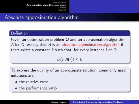
DefinitionGiven an optimization problem O and an approximation algorithmA for O, we say that A is an absolute approximation algorithm ifthere exists a constant k such that, for every instance i of O,
D(i , A(i)) ≤ k
To express the quality of an approximate solution, commonly usednotations are:
the relative errorthe performance ratio
Stefan Kugele Complexity Classes for Optimization Problems
IntroductionApproximation algorithms and errors
ClassesOutlook
Absolute approximation algorithm
DefinitionGiven an optimization problem O and an approximation algorithmA for O, we say that A is an absolute approximation algorithm ifthere exists a constant k such that, for every instance i of O,
D(i , A(i)) ≤ k
To express the quality of an approximate solution, commonly usednotations are:
the relative errorthe performance ratio
Stefan Kugele Complexity Classes for Optimization Problems

IntroductionApproximation algorithms and errors
ClassesOutlook
Relative error
DefinitionGiven an optimization problem O, for any instance i of O and forany feasible solution s of i , the relative error with respect to i isdefined as
E (i , s) =|m∗(i)−m(i , s)|
max {m∗(i), m(i , s)}For both, maximization and minimization problems, the relativeerror is equal to 0 when the solution obtained is optimal, andbecomes close to 1 when the approximate solution is very poor.
Stefan Kugele Complexity Classes for Optimization Problems
IntroductionApproximation algorithms and errors
ClassesOutlook
ε–approximate algorithm
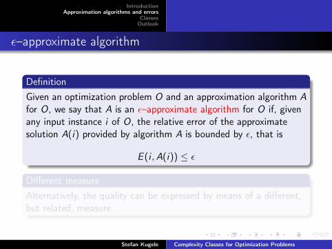
DefinitionGiven an optimization problem O and an approximation algorithm Afor O, we say that A is an ε–approximate algorithm for O if, givenany input instance i of O, the relative error of the approximatesolution A(i) provided by algorithm A is bounded by ε, that is
E (i , A(i)) ≤ ε
Different measureAlternatively, the quality can be expressed by means of a different,but related, measure.
Stefan Kugele Complexity Classes for Optimization Problems

IntroductionApproximation algorithms and errors
ClassesOutlook
ε–approximate algorithm
DefinitionGiven an optimization problem O and an approximation algorithm Afor O, we say that A is an ε–approximate algorithm for O if, givenany input instance i of O, the relative error of the approximatesolution A(i) provided by algorithm A is bounded by ε, that is
E (i , A(i)) ≤ ε
Different measureAlternatively, the quality can be expressed by means of a different,but related, measure.
Stefan Kugele Complexity Classes for Optimization Problems

IntroductionApproximation algorithms and errors
ClassesOutlook
Performance ratio
DefinitionGiven an optimization problem O, for any instance i of O and forany feasible solution s of i , the performance ratio of s with respectto i is defined as
R(i , s) = max
m(i , s)m∗(i)︸ ︷︷ ︸
min
,m∗(i)m(i , s)︸ ︷︷ ︸
max
For both, minimization and maximization, the value of theperformance ratio is equal to 1 in the case of an optimal solution,and can assume arbitrarily large values in the case of an poorapproximate solution.
Stefan Kugele Complexity Classes for Optimization Problems

IntroductionApproximation algorithms and errors
ClassesOutlook
r–approximate algorithm
DefinitionGiven an optimization problem O and an approximation algorithmA for O, we say that A is an r–approximate algorithm for O, givenany input instance i of O, the performance ratio of the approximatesolution A(i) is bounded by r , that is
R(i , A(i)) ≤ r
Relationship
E (i , s) = 1− 1R(i , s)
R(i , s) = − 1E (i , s)− 1
Stefan Kugele Complexity Classes for Optimization Problems

IntroductionApproximation algorithms and errors
ClassesOutlook
Example: E (i , s), R(i , s) for MinimumVertexCover
→ Flipchart
Stefan Kugele Complexity Classes for Optimization Problems

IntroductionApproximation algorithms and errors
ClassesOutlook
NPOAPXPTAS and FPT ASF −APXNegative Results
Outline
1 Approximation algorithms and errors
2 ClassesNPOAPXPT AS and FPT ASF −APXNegative Results
3 OutlookAP-ReductionsMaxSNP
Stefan Kugele Complexity Classes for Optimization Problems

IntroductionApproximation algorithms and errors
ClassesOutlook
NPOAPXPTAS and FPT ASF −APXNegative Results
The class NPO
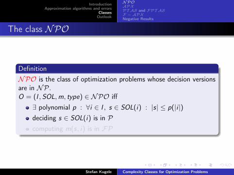
DefinitionNPO is the class of optimization problems whose decision versionsare in NP.O = (I , SOL, m, type) ∈ NPO iff
∃ polynomial p : ∀i ∈ I , s ∈ SOL(i) : |s| ≤ p(|i |)deciding s ∈ SOL(i) is in Pcomputing m(s, i) is in FP
Stefan Kugele Complexity Classes for Optimization Problems

IntroductionApproximation algorithms and errors
ClassesOutlook
NPOAPXPTAS and FPT ASF −APXNegative Results
The class NPO
DefinitionNPO is the class of optimization problems whose decision versionsare in NP.O = (I , SOL, m, type) ∈ NPO iff
∃ polynomial p : ∀i ∈ I , s ∈ SOL(i) : |s| ≤ p(|i |)deciding s ∈ SOL(i) is in Pcomputing m(s, i) is in FP
Stefan Kugele Complexity Classes for Optimization Problems

IntroductionApproximation algorithms and errors
ClassesOutlook
NPOAPXPTAS and FPT ASF −APXNegative Results
The class APX
DefinitionAPX is the class of all NPO problems such that, for some r ≥ 1,there exists a polynomial-time r -approximate algorithm for O.
InclusionsAPX ⊂ NPO ⇔ P 6= NP
Example
MinVertexCover, MaxSat, MaxKnapsack, MaxCut, MaxBinPacking,MaxPlanarGraphColoring
Stefan Kugele Complexity Classes for Optimization Problems

IntroductionApproximation algorithms and errors
ClassesOutlook
NPOAPXPTAS and FPT ASF −APXNegative Results
The class APX (cont.)
Proof.Idee: TSP can not be r -approximated, no matter how large isthe performance ratio r .Reduction from the NP-complete HamiltonianCircuit decisionproblem.Let G = (V , E ) be an instance of HC with |V | = n.Construct for any r ≥ 1 a MinTSP instance such that if wehad a poly-time r -approximate algorithms for MinTSP, thenwe could decide whether the graph G has a HC in polynomialtime.
Stefan Kugele Complexity Classes for Optimization Problems

IntroductionApproximation algorithms and errors
ClassesOutlook
NPOAPXPTAS and FPT ASF −APXNegative Results
The class APX (cont.)
Proof (cont.)
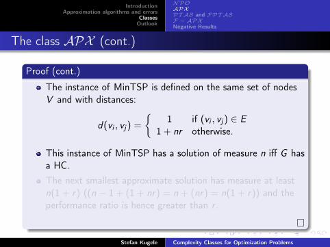
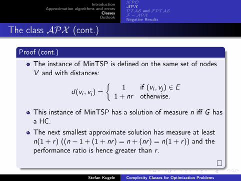
The instance of MinTSP is defined on the same set of nodesV and with distances:
d(vi , vj) =
{1 if (vi , vj) ∈ E
1 + nr otherwise.
This instance of MinTSP has a solution of measure n iff G hasa HC.The next smallest approximate solution has measure at leastn(1 + r) ((n − 1 + (1 + nr) = n + (nr) = n(1 + r)) and theperformance ratio is hence greater than r .
Stefan Kugele Complexity Classes for Optimization Problems
IntroductionApproximation algorithms and errors
ClassesOutlook
NPOAPXPTAS and FPT ASF −APXNegative Results
The class APX (cont.)
Proof (cont.)
The instance of MinTSP is defined on the same set of nodesV and with distances:
d(vi , vj) =
{1 if (vi , vj) ∈ E
1 + nr otherwise.
This instance of MinTSP has a solution of measure n iff G hasa HC.The next smallest approximate solution has measure at leastn(1 + r) ((n − 1 + (1 + nr) = n + (nr) = n(1 + r)) and theperformance ratio is hence greater than r .
Stefan Kugele Complexity Classes for Optimization Problems

IntroductionApproximation algorithms and errors
ClassesOutlook
NPOAPXPTAS and FPT ASF −APXNegative Results
The class APX (cont.)
Proof (cont.)
If G has no HC, then the optimal solution has measure at leastn(1 + r).Therefore, if we had a polynomial r -approximate algorithm forMinTSP, we could use it to decide whether G has a HC in thefollowing way: apply the approximation algorithm to theinstance of MinTSP and answer YES iff it returns a solutionof measure n.
Stefan Kugele Complexity Classes for Optimization Problems

IntroductionApproximation algorithms and errors
ClassesOutlook
NPOAPXPTAS and FPT ASF −APXNegative Results
Example: MinimumVertexCover
Example (MinimumVertexCover)
Instance: Graph G = (V , E )
Query: Smallest vertex coverTheorm: MinimumVertexCover is 2-approximatable, that is
MinimumVertexCover ∈ APXProof: The corresponding decision problem is NP-complete
Stefan Kugele Complexity Classes for Optimization Problems

IntroductionApproximation algorithms and errors
ClassesOutlook
NPOAPXPTAS and FPT ASF −APXNegative Results
Example: MinimumVertexCover (cont.)
Algorithm MinimumVertexCover
procedure VertexCover-2-Approx(V , E )while E 6= ∅ do
pick an arbitrary edge {u, v} ∈ Eadd u and v to the vertex coverdelete all edges covered by u and v from E
end whileend procedure
Stefan Kugele Complexity Classes for Optimization Problems

IntroductionApproximation algorithms and errors
ClassesOutlook
NPOAPXPTAS and FPT ASF −APXNegative Results
Example: MinimumVertexCover (cont.)
Algorithm MinimumVertexCover
while E 6= ∅ dopick an arbitrary edge {u, v} ∈ Eadd u and v to the vertex coverdelete edges covered by u and v from E
end while
Trace
VC = {}E = {(A, G ), (A, E ), (A, D), (A, C ),(B, G ), (B, F ), (B, D), (B, C ),(D, G ), (D, F )}
Stefan Kugele Complexity Classes for Optimization Problems

IntroductionApproximation algorithms and errors
ClassesOutlook
NPOAPXPTAS and FPT ASF −APXNegative Results
Example: MinimumVertexCover (cont.)
Algorithm MinimumVertexCover
while E 6= ∅ dopick an arbitrary edge {u, v} ∈ E .add u and v to the vertex coverdelete edges covered by u and v from E
end while
Trace
VC = {}E = {(A, G ), (A, E ), (A, D), (A, C ),(B, G ), (B, F ), (B, D), (B, C ),(D, G ), (D, F )}
Stefan Kugele Complexity Classes for Optimization Problems

IntroductionApproximation algorithms and errors
ClassesOutlook
NPOAPXPTAS and FPT ASF −APXNegative Results
Example: MinimumVertexCover (cont.)
Algorithm MinimumVertexCover
while E 6= ∅ dopick an arbitrary edge {u, v} ∈ Eadd u and v to the vertex cover .delete edges covered by u and v from E
end while
Trace
VC = {A, D}E = {(A, G ), (A, E ), (A, D), (A, C ),(B, G ), (B, F ), (B, D), (B, C ),(D, G ), (D, F )}
Stefan Kugele Complexity Classes for Optimization Problems

IntroductionApproximation algorithms and errors
ClassesOutlook
NPOAPXPTAS and FPT ASF −APXNegative Results
Example: MinimumVertexCover (cont.)
Algorithm MinimumVertexCover
while E 6= ∅ dopick an arbitrary edge {u, v} ∈ Eadd u and v to the vertex coverdelete edges covered by u and v from E.
end while
Trace
VC = {A, D}E = {(A, G ), (A, E ), (A, D), (A, C ),(B, G ), (B, F ), (B, D), (B, C ),(D, G ), (D, F )}
Stefan Kugele Complexity Classes for Optimization Problems

IntroductionApproximation algorithms and errors
ClassesOutlook
NPOAPXPTAS and FPT ASF −APXNegative Results
Example: MinimumVertexCover (cont.)
Algorithm MinimumVertexCover
while E 6= ∅ dopick an arbitrary edge {u, v} ∈ E .add u and v to the vertex coverdelete edges covered by u and v from E
end while
Trace
VC = {A, D}E = {(B, G ), (B, F ), (B, C )}
Stefan Kugele Complexity Classes for Optimization Problems

IntroductionApproximation algorithms and errors
ClassesOutlook
NPOAPXPTAS and FPT ASF −APXNegative Results
Example: MinimumVertexCover (cont.)
Algorithm MinimumVertexCover
while E 6= ∅ dopick an arbitrary edge {u, v} ∈ Eadd u and v to the vertex cover .delete edges covered by u and v from E
end while
Trace
VC = {A, D, B, G}E = {(B, G ), (B, F ), (B, C )}
Stefan Kugele Complexity Classes for Optimization Problems

IntroductionApproximation algorithms and errors
ClassesOutlook
NPOAPXPTAS and FPT ASF −APXNegative Results
Example: MinimumVertexCover (cont.)
Algorithm MinimumVertexCover
while E 6= ∅ dopick an arbitrary edge {u, v} ∈ Eadd u and v to the vertex coverdelete edges covered by u and v from E.
end while
Trace
VC = {A, D, B, G}E = {(B, G ), (B, F ), (B, C )}
Stefan Kugele Complexity Classes for Optimization Problems

IntroductionApproximation algorithms and errors
ClassesOutlook
NPOAPXPTAS and FPT ASF −APXNegative Results
Example: MinimumVertexCover (cont.)
Algorithm MinimumVertexCover
while E 6= ∅ dopick an arbitrary edge {u, v} ∈ Eadd u and v to the vertex coverdelete edges covered by u and v from E
end while
Trace
VC = {A, D, B, G} ← 2− approx .resultE = {}
Stefan Kugele Complexity Classes for Optimization Problems

IntroductionApproximation algorithms and errors
ClassesOutlook
NPOAPXPTAS and FPT ASF −APXNegative Results
Example: MinimumVertexCover (cont.)
Stefan Kugele Complexity Classes for Optimization Problems

IntroductionApproximation algorithms and errors
ClassesOutlook
NPOAPXPTAS and FPT ASF −APXNegative Results
Example: MinimumVertexCover (cont.)
QuestionThe result is a vertex cover but is its size maximum twice theoptimum?
AnswerYes. No two edges chosen by the algorithm have shared nodes.Hence, a vertex cover of only those edges has to contain at leasteither of them, i.e. be at least half of the size of the found vertexcover.
Stefan Kugele Complexity Classes for Optimization Problems

IntroductionApproximation algorithms and errors
ClassesOutlook
NPOAPXPTAS and FPT ASF −APXNegative Results
Inclusions so far (P 6= NP)
Stefan Kugele Complexity Classes for Optimization Problems

IntroductionApproximation algorithms and errors
ClassesOutlook
NPOAPXPTAS and FPT ASF −APXNegative Results
Limits to approximability: The gap technique
TheoremLet O’ be an NP-complete decision problem and let O be anNPO minimization problem. Let us suppose that there exist twopolynomial-time computable functions
f : IO′ 7→ IOc : IO′ 7→ N
a constant gap > 0, such that for any instamce i of O ′,
m∗(f (i)) =
{c(i) if i is a positive instance
c(i)(1 + gap) otherwise.
Then no polynomial-time r-approximate algorithm for O withr < 1 + gap can exist, unless P = NP.
Stefan Kugele Complexity Classes for Optimization Problems

IntroductionApproximation algorithms and errors
ClassesOutlook
NPOAPXPTAS and FPT ASF −APXNegative Results
Limits to approximability: The gap technique (cont.)
Proof.→ Flipchart
Stefan Kugele Complexity Classes for Optimization Problems

IntroductionApproximation algorithms and errors
ClassesOutlook
NPOAPXPTAS and FPT ASF −APXNegative Results
Limits to approximability: The gap technique (cont.)
Example (1)
Given a planar graph decide whether this graph is 3-colorable. Thisproblem is NP-complete. But any planar graph can be coloredwith 4 colors.Define f as the identity function: f (G ) = G is a planar graph
If G is 3-colorable, then m∗(f (G )) = 3If G is not 3-colorable, then m∗(f (G )) = 4 = 3(1 + 1
3)
gap = 13
Theorem
MinimumGraphColoring has no r-approximate algorithm with r < 43
unless P = NP.
Stefan Kugele Complexity Classes for Optimization Problems

IntroductionApproximation algorithms and errors
ClassesOutlook
NPOAPXPTAS and FPT ASF −APXNegative Results
Limits to approximability: The gap technique (cont.)
Example (2)
MinimumBinPacking→ Flipchart
Stefan Kugele Complexity Classes for Optimization Problems

IntroductionApproximation algorithms and errors
ClassesOutlook
NPOAPXPTAS and FPT ASF −APXNegative Results
Polynomial-time approximation schemes (PT AS)
DefinitionLet O be an NPO problem. An algorithm A is said to be apolynomial time approximation scheme (PT AS) for O if, for anyinstance i of O and any rational value r > 1, A when applied toinput (i , r) returns an r -approximate solution of i in timepolynomial in |i |.
The running time of a PT AS may also depend exponentiallyon 1
r−1
The better the approximation, the larger may be the runningtime
Stefan Kugele Complexity Classes for Optimization Problems

IntroductionApproximation algorithms and errors
ClassesOutlook
NPOAPXPTAS and FPT ASF −APXNegative Results
The class PT AS
DefinitionPT AS is the class of NPO problems that admit apolynomial-time approximation scheme.
Example
MaxIntegerKnapsack, MaxIndependentSet (for planar graphs)
InclusionsPT AS ⊂ APX ⇔ P 6= NP
In some cases, the increase in the running time of theapproximation scheme with the degree of approximation mayprevent any practical use of the scheme.
Stefan Kugele Complexity Classes for Optimization Problems

IntroductionApproximation algorithms and errors
ClassesOutlook
NPOAPXPTAS and FPT ASF −APXNegative Results
The class PT AS (cont.)
Proof.Already done. MinimumBinPacking-exampleMinimumBinPacking has no r -approximate algorithm withr < 3
2 unless P = NP.Therefore, unless P = NP, MinimumBinPacking does notadmit a PT AS.
Stefan Kugele Complexity Classes for Optimization Problems

IntroductionApproximation algorithms and errors
ClassesOutlook
NPOAPXPTAS and FPT ASF −APXNegative Results
Inclusions so far (P 6= NP)
Stefan Kugele Complexity Classes for Optimization Problems

IntroductionApproximation algorithms and errors
ClassesOutlook
NPOAPXPTAS and FPT ASF −APXNegative Results
Fully polinomial-time approximation scheme (FPT AS)
A much better situation would arise when the running time ispolynomial both in the size of the input and in the inverse of theperformance ratio.
DefinitionLet O be an NPO problem. An algorithms is said to be a fullypolynomial time approximation scheme (FPT AS) for O if, for anyinstance i of O and for any rational value r > 1, A when applied toinput (i , r) returns an r -approximate solution of i in timepolynomial both in |i | and 1
(r−1) .
Stefan Kugele Complexity Classes for Optimization Problems

IntroductionApproximation algorithms and errors
ClassesOutlook
NPOAPXPTAS and FPT ASF −APXNegative Results
The class FPT AS
DefinitionFPT AS is the class of NPO problems that admit a fullypolynomial-time approximation scheme.
Example
MaximumKnapsack
InclusionsFPT AS ⊂ PT AS ⇔ P 6= NP
Stefan Kugele Complexity Classes for Optimization Problems

IntroductionApproximation algorithms and errors
ClassesOutlook
NPOAPXPTAS and FPT ASF −APXNegative Results
The class FPT AS (cont.)
Proof.Some hints:
MaximumIndependentSetpolynomially bounded
Later, if you want to ;-)
Stefan Kugele Complexity Classes for Optimization Problems
IntroductionApproximation algorithms and errors
ClassesOutlook
NPOAPXPTAS and FPT ASF −APXNegative Results
The class FPT AS (cont.)
Proof.Some hints:
MaximumIndependentSetpolynomially bounded
Later, if you want to ;-)
Stefan Kugele Complexity Classes for Optimization Problems

IntroductionApproximation algorithms and errors
ClassesOutlook
NPOAPXPTAS and FPT ASF −APXNegative Results
The class FPT AS (cont.)
Proof.Some hints:
MaximumIndependentSetpolynomially bounded
Later, if you want to ;-)
Stefan Kugele Complexity Classes for Optimization Problems

IntroductionApproximation algorithms and errors
ClassesOutlook
NPOAPXPTAS and FPT ASF −APXNegative Results
The class FPT AS (cont.)
Proof.Some hints:
MaximumIndependentSetpolynomially bounded
Later, if you want to ;-)
Stefan Kugele Complexity Classes for Optimization Problems

IntroductionApproximation algorithms and errors
ClassesOutlook
NPOAPXPTAS and FPT ASF −APXNegative Results
Inclusions so far (P 6= NP)
Stefan Kugele Complexity Classes for Optimization Problems

IntroductionApproximation algorithms and errors
ClassesOutlook
NPOAPXPTAS and FPT ASF −APXNegative Results
F −APX
DefinitionLet O be an NPO problem. O is said to be in F −APX if andonly if there exists an f -approximation algorithm A for O whichruns in polynomial-time for some function f ∈ F .
InclusionsFPT AS ⊂ PT AS ⊂ APX ⊂ log −APX ⊂ poly −APX ⊂
exp −APX ⊂ NPO ⇔ P 6= NP
Stefan Kugele Complexity Classes for Optimization Problems

IntroductionApproximation algorithms and errors
ClassesOutlook
NPOAPXPTAS and FPT ASF −APXNegative Results
F −APX (cont.)
Example
APX Max3Satlog−APX SetCover
poly −APX Coloringexp−APX TSP
Stefan Kugele Complexity Classes for Optimization Problems

IntroductionApproximation algorithms and errors
ClassesOutlook
NPOAPXPTAS and FPT ASF −APXNegative Results
F −APX (cont.)
Example
APX Max3Satlog−APX SetCover
poly −APX Coloringexp−APX TSP
Stefan Kugele Complexity Classes for Optimization Problems

IntroductionApproximation algorithms and errors
ClassesOutlook
NPOAPXPTAS and FPT ASF −APXNegative Results
F −APX (cont.)
Example
APX Max3Satlog−APX SetCover
poly −APX Coloringexp−APX TSP
Stefan Kugele Complexity Classes for Optimization Problems

IntroductionApproximation algorithms and errors
ClassesOutlook
NPOAPXPTAS and FPT ASF −APXNegative Results
F −APX (cont.)
Example
APX Max3Satlog−APX SetCover
poly −APX Coloringexp−APX TSP
Stefan Kugele Complexity Classes for Optimization Problems

IntroductionApproximation algorithms and errors
ClassesOutlook
NPOAPXPTAS and FPT ASF −APXNegative Results
Inclusions so far (P 6= NP)
Stefan Kugele Complexity Classes for Optimization Problems

IntroductionApproximation algorithms and errors
ClassesOutlook
NPOAPXPTAS and FPT ASF −APXNegative Results
Polynomially bounded optimization problems
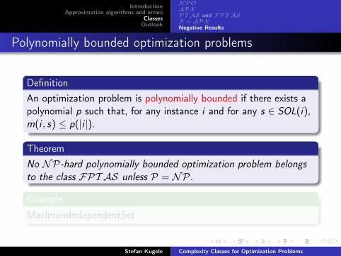
DefinitionAn optimization problem is polynomially bounded if there exists apolynomial p such that, for any instance i and for any s ∈ SOL(i),m(i , s) ≤ p(|i |).
TheoremNo NP-hard polynomially bounded optimization problem belongsto the class FPT AS unless P = NP.
Example
MaximumIndependentSet
Stefan Kugele Complexity Classes for Optimization Problems
IntroductionApproximation algorithms and errors
ClassesOutlook
NPOAPXPTAS and FPT ASF −APXNegative Results
Polynomially bounded optimization problems
DefinitionAn optimization problem is polynomially bounded if there exists apolynomial p such that, for any instance i and for any s ∈ SOL(i),m(i , s) ≤ p(|i |).
TheoremNo NP-hard polynomially bounded optimization problem belongsto the class FPT AS unless P = NP.
Example
MaximumIndependentSet
Stefan Kugele Complexity Classes for Optimization Problems

IntroductionApproximation algorithms and errors
ClassesOutlook
NPOAPXPTAS and FPT ASF −APXNegative Results
Polynomially bounded optimization problems (cont.)
Proof.→ Flipchart
Stefan Kugele Complexity Classes for Optimization Problems

IntroductionApproximation algorithms and errors
ClassesOutlook
NPOAPXPTAS and FPT ASF −APXNegative Results
Pseudo-polynomial problem
DefinitionAn NPO problem O is pseudo-polynomial if it can be solved by analgorithm that, on any instance i , runs in time bounded by apolynomial in |i | and in max(i), where max(i) denotes the value ofthe largest number occurring in i .
TheoremLet O be an NPO problem in FPT AS. If a polynomial p existssuch that, for every input i , m∗(x) ≤ p(|i |), max(i)), then O is apseudo-polynomial problem.
Example
MaximumKnapsack: max(i) = max{a1, ..., an, p1, ..., pn}
Stefan Kugele Complexity Classes for Optimization Problems

IntroductionApproximation algorithms and errors
ClassesOutlook
NPOAPXPTAS and FPT ASF −APXNegative Results
Strongly NP-hard problem
Let O be an NPO problem and let p be a polynomial. We denoteby Omax ,p the problem obtained by restricting O to only thoseinstances i which max(i) ≤ p(|i |).
DefinitionAn NPO problem O is said to be strongly NP-hard if apolynomial p exists such that Omax ,p is NP-hard.
Stefan Kugele Complexity Classes for Optimization Problems

IntroductionApproximation algorithms and errors
ClassesOutlook
NPOAPXPTAS and FPT ASF −APXNegative Results
Strongly NP-hard problem (cont.)
TheoremIf P 6= NP, then no strongly NP-hard problem can bepseudo-polynomial.
Proof.→ Flipchart
From the last two theorems, the following result can be derived.Let O be a strongly NP-hard problem that admits a polynomial psuch that m∗(i) ≤ p(|i |, max(i)), for every input i . If P 6= NP,then O does not belong to the class FPT AS.
Stefan Kugele Complexity Classes for Optimization Problems

IntroductionApproximation algorithms and errors
ClassesOutlook
NPOAPXPTAS and FPT ASF −APXNegative Results
Negative results for the class FPT AS
Negative results
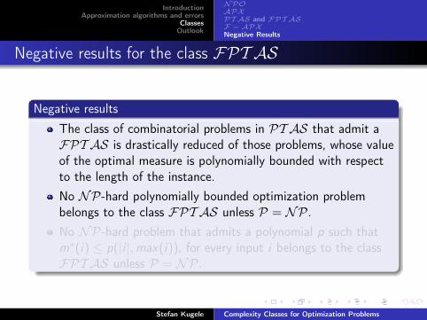
The class of combinatorial problems in PT AS that admit aFPT AS is drastically reduced of those problems, whose valueof the optimal measure is polynomially bounded with respectto the length of the instance.No NP-hard polynomially bounded optimization problembelongs to the class FPT AS unless P = NP.No NP-hard problem that admits a polynomial p such thatm∗(i) ≤ p(|i |, max(i)), for every input i belongs to the classFPT AS unless P = NP.
Stefan Kugele Complexity Classes for Optimization Problems

IntroductionApproximation algorithms and errors
ClassesOutlook
NPOAPXPTAS and FPT ASF −APXNegative Results
Negative results for the class FPT AS
Negative results
The class of combinatorial problems in PT AS that admit aFPT AS is drastically reduced of those problems, whose valueof the optimal measure is polynomially bounded with respectto the length of the instance.No NP-hard polynomially bounded optimization problembelongs to the class FPT AS unless P = NP.No NP-hard problem that admits a polynomial p such thatm∗(i) ≤ p(|i |, max(i)), for every input i belongs to the classFPT AS unless P = NP.
Stefan Kugele Complexity Classes for Optimization Problems

IntroductionApproximation algorithms and errors
ClassesOutlook
AP-ReductionsMaxSNP
Outline
1 Approximation algorithms and errors
2 ClassesNPOAPXPT AS and FPT ASF −APXNegative Results
3 OutlookAP-ReductionsMaxSNP
Stefan Kugele Complexity Classes for Optimization Problems

IntroductionApproximation algorithms and errors
ClassesOutlook
AP-ReductionsMaxSNP
Approximation Preserving Reductions
DefinitionLet O1 and O2 be two optimization problems in NPO. O1 is saidto be AP-reducible to O2, in symbol O1 ≤AP O2, if two functions fand g and a positive constant α ≥ 1 exist such that:
For any instance i ∈ IO1 and for any rational r > 1,f (i , r) ∈ IO2 .
For any instance i ∈ IO1 and for any rational r > 1, ifSOLO1(i) 6= ∅ then SOLO2(f (i , r)) 6= ∅.For any instance i ∈ IO1 , for any rational r > 1, and for anyy ∈ SOLO2(f (i , r)), g(i , y , r) ∈ SOLO1(i).
Stefan Kugele Complexity Classes for Optimization Problems
IntroductionApproximation algorithms and errors
ClassesOutlook
AP-ReductionsMaxSNP
Approximation Preserving Reductions (cont.)
Definition (cont.)
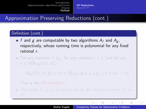
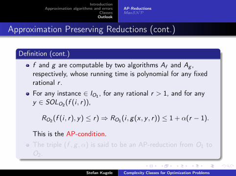
f and g are computable by two algorithms Af and Ag ,respectively, whose running time is polynomial for any fixedrational r .For any instance ∈ IO1 , for any rational r > 1, and for anyy ∈ SOLO2(f (i , r)),
RO2(f (i , r), y) ≤ r)⇒ RO1(i , g(x , y , r)) ≤ 1 + α(r − 1).
This is the AP-condition.The triple (f , g , α) is said to be an AP-reduction from O1 toO2.
Stefan Kugele Complexity Classes for Optimization Problems
IntroductionApproximation algorithms and errors
ClassesOutlook
AP-ReductionsMaxSNP
Approximation Preserving Reductions (cont.)
Definition (cont.)
f and g are computable by two algorithms Af and Ag ,respectively, whose running time is polynomial for any fixedrational r .For any instance ∈ IO1 , for any rational r > 1, and for anyy ∈ SOLO2(f (i , r)),
RO2(f (i , r), y) ≤ r)⇒ RO1(i , g(x , y , r)) ≤ 1 + α(r − 1).
This is the AP-condition.The triple (f , g , α) is said to be an AP-reduction from O1 toO2.
Stefan Kugele Complexity Classes for Optimization Problems

IntroductionApproximation algorithms and errors
ClassesOutlook
AP-ReductionsMaxSNP
AP-Reduction (cont.)
Stefan Kugele Complexity Classes for Optimization Problems

IntroductionApproximation algorithms and errors
ClassesOutlook
AP-ReductionsMaxSNP
AP-Reduction (cont.)
LemmaIf O1 ≤AP O2 and O2 ∈ APX (respectively, O2 ∈ PT AS), thenO1 ∈ APX (respectively, O1 ∈ PT AS).
Proof.→ Flipchart
Example
MaximumClique ≤AP MaximumIndependentSet
Stefan Kugele Complexity Classes for Optimization Problems

IntroductionApproximation algorithms and errors
ClassesOutlook
AP-ReductionsMaxSNP
Fagin’s Theorem (1974)
Fagin, Ron, IBM
TheoremA property is expressible in existentialsecond-order logic (∃SO) iff it isdecidable in NP.
Stefan Kugele Complexity Classes for Optimization Problems

IntroductionApproximation algorithms and errors
ClassesOutlook
AP-ReductionsMaxSNP
The class SNP (strictNP)
SNPThe class SNP consists of all properties expressible as
∃S∀x1∀x2 . . .∀xkϕ(S , G , x1, . . . , xk)
ϕ is a quantifier-free First-Order expression involving thevariables xi and the structures G and S .G is the input, S is the demanded relation that satisfies ϕ
Modificationsϕ holds not for all k-tuples of nodes (x1, . . . , xk), instead weseek the relation S such that ϕ holds for as many k-tuples(x1, . . . , xk) as possible.G now is a collection G1, . . . , Gm of relations of arbitrary arity.
Stefan Kugele Complexity Classes for Optimization Problems

IntroductionApproximation algorithms and errors
ClassesOutlook
AP-ReductionsMaxSNP
The classes MaxSNP0 and MaxSNP
MaxSNP0
maxS
∣∣∣{(x1, . . . , xk) ∈ V k : ϕ(G1, . . . , Gm, S , x1, . . . , xk)}∣∣∣
DefinitionMaxSNP is the class of all optimization problems that areL-reducible to a problem in MaxSNP0
Introduced in 1989 by Papadimitriou and YannakakisThey showed, that all problems in MaxSNP are in APXYou can get an approximation algorithm canonical out of theproblem definition using ϕ
Stefan Kugele Complexity Classes for Optimization Problems