Imperial College London

BSc Project

Complex Processes and 3D Printing

Author:Dominic Reiss

Supervisor:Dr. Tim Evans

Partner:Joshua Price

June 10, 2013

Acknowledgement

I would like to express my special gratitude to my supervisor, Dr. Tim Evans, for motivation and guidancethroughout the project, as well as my project partner, Joshua Price, for his hard work and excellent co-operation.

I would also like to thank the Imperial College Robotics Society, especially Thomas Clayson and AksatShah, for allowing us to use their Reprap 3D printer and for offering their expert advice on approaches to3D printing.

i

Abstract

A process which converts 2D evolving cellular automata into 3D printed objects was designed. Theprocess takes into account the limitations inherent to 3D printing processes and materials and bypasses theuse of CAD software and manual part design. Alongside the process itself, a software which automates thegreater part of this process was developed. A physical model of a cellular automaton was successfully printedand suggests that in the future a process similar to the one developed in this project may be used to convertphysics models into 3D objects.

ii

Contents

1 Introduction and Background 11.1 Overview of 3D Printing Technologies . . . . . . . . . . . . . . . . . . . . . . . . . . . . . . . . . 1

1.1.1 Recent History and Advances . . . . . . . . . . . . . . . . . . . . . . . . . . . . . . . . . . 11.1.2 Common 3D Printing Processes . . . . . . . . . . . . . . . . . . . . . . . . . . . . . . . . . 21.1.3 Common 3D Printing Materials . . . . . . . . . . . . . . . . . . . . . . . . . . . . . . . . . 31.1.4 Limitations of Processes and Materials . . . . . . . . . . . . . . . . . . . . . . . . . . . . . 31.1.5 Part Design . . . . . . . . . . . . . . . . . . . . . . . . . . . . . . . . . . . . . . . . . . . . 41.1.6 STL Files . . . . . . . . . . . . . . . . . . . . . . . . . . . . . . . . . . . . . . . . . . . . . 4

1.2 Overview of Cellular Automata . . . . . . . . . . . . . . . . . . . . . . . . . . . . . . . . . . . . . 51.2.1 Definition and Basic Properties . . . . . . . . . . . . . . . . . . . . . . . . . . . . . . . . . 51.2.2 Deterministic Models . . . . . . . . . . . . . . . . . . . . . . . . . . . . . . . . . . . . . . 51.2.3 Probabilistic Models . . . . . . . . . . . . . . . . . . . . . . . . . . . . . . . . . . . . . . . 61.2.4 Physical Relevance . . . . . . . . . . . . . . . . . . . . . . . . . . . . . . . . . . . . . . . . 7

2 Motivation and Objectives 7

3 Anticipated Obstacles and Proposed Solutions 73.1 Support Constraint . . . . . . . . . . . . . . . . . . . . . . . . . . . . . . . . . . . . . . . . . . . . 83.2 Overhang Angle Constraint . . . . . . . . . . . . . . . . . . . . . . . . . . . . . . . . . . . . . . . 93.3 Stability Constraint . . . . . . . . . . . . . . . . . . . . . . . . . . . . . . . . . . . . . . . . . . . 9

4 Equipment and Technologies 9

5 Description of Software Developed 115.1 Lattice and Iterative Model Structures . . . . . . . . . . . . . . . . . . . . . . . . . . . . . . . . . 115.2 Lattice to Polyhedron Conversion . . . . . . . . . . . . . . . . . . . . . . . . . . . . . . . . . . . . 125.3 GUI Elements . . . . . . . . . . . . . . . . . . . . . . . . . . . . . . . . . . . . . . . . . . . . . . . 12

6 Achievements and Results 12

7 Unexpected Issues and Potential Solutions 14

8 Extensions and Future Work 15

9 Conclusion 17

iii

List of Figures

1 An example of emergent 3D printed art: Fractal.MGX . . . . . . . . . . . . . . . . . . . . . . . . 12 The FDM extrusion process . . . . . . . . . . . . . . . . . . . . . . . . . . . . . . . . . . . . . . . 23 Example of a threshold overhanging angle . . . . . . . . . . . . . . . . . . . . . . . . . . . . . . . 44 Non-manifold edge . . . . . . . . . . . . . . . . . . . . . . . . . . . . . . . . . . . . . . . . . . . . 45 An example of a small lattice gas . . . . . . . . . . . . . . . . . . . . . . . . . . . . . . . . . . . . 56 Probabilistic nature of forest fire model . . . . . . . . . . . . . . . . . . . . . . . . . . . . . . . . 67 3D array of cubes visualisation . . . . . . . . . . . . . . . . . . . . . . . . . . . . . . . . . . . . . 88 Layers with little to no overlap . . . . . . . . . . . . . . . . . . . . . . . . . . . . . . . . . . . . . 99 Layers with half overlap . . . . . . . . . . . . . . . . . . . . . . . . . . . . . . . . . . . . . . . . . 1010 Stretched overlapping cubes . . . . . . . . . . . . . . . . . . . . . . . . . . . . . . . . . . . . . . . 1011 Smoothed overlapping cubes . . . . . . . . . . . . . . . . . . . . . . . . . . . . . . . . . . . . . . . 1112 Examples of options available in the GUI . . . . . . . . . . . . . . . . . . . . . . . . . . . . . . . 1313 Evolution of a cellular automaton in the GUI . . . . . . . . . . . . . . . . . . . . . . . . . . . . . 1414 3D example of 2D lattice gas expanding in time . . . . . . . . . . . . . . . . . . . . . . . . . . . . 1515 Rough and smooth 3D representations of a modified forest fire . . . . . . . . . . . . . . . . . . . 1516 Top-down view of a modified forest fire . . . . . . . . . . . . . . . . . . . . . . . . . . . . . . . . . 1617 Final printed modified forest fire . . . . . . . . . . . . . . . . . . . . . . . . . . . . . . . . . . . . 1618 Underside of model shows unexpected offset . . . . . . . . . . . . . . . . . . . . . . . . . . . . . . 17

iv

1 Introduction and Background

1.1 Overview of 3D Printing Technologies

1.1.1 Recent History and Advances

3D printing, also known as additive manufacturing, is the process of constructing a three dimensional objectthrough applications of successive layers of material. Additive manufacturing technologies are distinct whencompared to processes such as machining, which remove material to create features and are known as subtractiveprocesses [1]. While machining has been used in factories for decades, additive manufacturing techniques bringto the table benefits such as easy prototyping, increased geometric complexity, and versatility in design.

Charles Hull is often called the ‘Father of 3D printing’ as he invented stereo-lithography in 1984. In the threedecades since then major advances have been made and several new techniques have been developed [2]. In 2010,the additive manufacturing industry was estimated at $1.3B and this valuation only expected to increase in thenear future. These increases have led many companies and governments to invest in research and development of3D printing technologies [3]. Open source collaboration as well as a significant price decrease of the technologyhas ensured that 3D printing is becoming one of the most exciting and quickest growing technologies for thepresent and the future.

Additive manufacturing is a flexible process, able to produce many geometries in a wide range of materials, andin turn has a large number of applications. Rapid prototyping is a technique now used in the design stage of manyproducts, in which designers use additive manufacturing processes to quickly produce scale models of prototypedesigns at reasonable cost [1]. Another emerging use for additive manufacturing is direct digital manufacturing,where manufacturers use 3D printing to produce end-user products with benefits of easy customization and nothaving to produce inventory until an order is placed [4]. 3D printing has become a tool for hobbyists to createcustomized parts easily without having to buy them externally. 3D printing has also been used to produce 3Dart, many examples of which can be seen at the 3D Printshow which tours some of the biggest cities in theworld [5]. 3D art has also began making an appearance in art museums, a prime example of which is the pieceFractal.MGX recently acquired by the V&A Museum in London, depicted in figure 1 [6].

Figure 1: An example of emergent 3D printed art, titled Fractal.MGX, can be seen on display in the V&Amuseum in London. The reaches of additive manufacturing to areas such as art only reinforces the idea of itsdiversity in application. (Image taken from [6].)

1

1.1.2 Common 3D Printing Processes

There are four common types of 3D printing processes, each of which have fundamentally different ways ofbuilding up layers of material.

• Extrusion Deposition: This method normally consists of the deposition of melted thermoplastic inlayers. Most commonly a heated moveable bed is placed underneath a heated nozzle which extrudesmolten plastic onto the bed. Directions from a computer tell the nozzle how much to extrude and how thebed and nozzle should move with respect to each other in order to produce the desired part. The mostcommon form of extrusion deposition is called Fused Deposition Modeling (FDM), depicted in figure 2,which can create layers as thin as 0.04mm. FDM is currently one of the most popular 3D printing methodsas it is very affordable, easy to install, and creates quite complex geometries. The major disadvantage ofFDM is that printing large overhangs is often not possible and requires support structures. [1] [7]

Figure 2: The FDM extrusion process. 1 - Nozzle extruding molten plastic. 2 - Layers of material. 3 -Moveable heated bed. (Image taken from [8].)

• Granular Materials Binding: This method fuses granular materials layer by layer until the structureis built up. To do this a layer of granular material is spread evenly over a bed. Selected sections of thisgranular layer are fused by complete or partial melting, using a laser or heating element. This processis repeated to form the entire object. The most common form of granular materials binding is knownas selective laser sintering (SLS), in which a laser is used to fuse the granular particles. SLS can use awide range of granular materials, including types of plastics, metals, ceramics, and glass, and can producestructures with a high geometric complexity and significant overhangs. The disadvantages of SLS includethe resolution of the object being limited to the material’s granule size. [1] [9]

• Laminated Object Manufacturing (LOM): This process involves layer-by-layer lamination of sheetsof material. Each layer is cut using a CO2 laser, removing the unwanted material. The most commonmaterial for LOM is paper, coated on one side by a thermoplastic. LOM was very popular in the 90s whenit was used commercially, however its popularity is now waning with the emergence of FDM and SLS. [1]

• Photo-polymerisation: This class of processes exposes photo-polymers to radiation (typically ultravio-let). The radiation triggers a chemical reaction within the material, causing the material to become solid.Stereo-lithography (SLA) was developed in the mid-80s, in which layers of UV curable liquids are formedover one another. Since then, many new types of radiation curable materials have been commerciallydeveloped, expanding SLA. SLA is mainly used for its variety in commercial photo-polymers, and is themain method of bio-printing (which aims to 3D print organs and tissue). Downsides to SLA are costs and

2

the choice of materials being limited to photo-polymer materials. [1]

1.1.3 Common 3D Printing Materials

There are three common material types used for 3D printing. The material used in a design often characterizesthe manufacturing process, as many 3D printing processes are limited to a few types of materials.

• Thermoplastics: These synthetic resins become pliable when heated, and are currently the most commonclass of material used in 3D printing. Plastics known as ABS and polycarbonate (PC) are most often used,however a number of blends and plastics engineered for specific applications (such as aerospace or medical)also exist. Thermoplastics are sturdy and can be used either for end-user products or for prototypingpurposes. FDM and SLS processes can both employ thermoplastics. [1] [10]

• Metals: More recently, innovations in granular binding have made metals viable for 3D printing. SLSand similar processes can fuse metal granules, such as steel and titanium. Metals are especially useful forspecific applications such as electrical components, jewellery, and engineering support structures. [1]

• Photo-polymers: This class of polymers change their properties, typically by changing from a liquidstate to a solid, when exposed to specific frequencies of radiation. Various types of radiation may beused, however in commercial environments today only UV and visible frequencies are commonly used.Photo-polymers are only used in photo-polymerisation processes such as SLA, and are typically hybridsof epoxy and acrylic resins. [1] [11]

• Other Materials: Granular processes can theoretically work with any fuseable granular material. Asidefrom thermoplastics and metals, materials such as glass, nylons, and polystyrene have been used in SLSprinting. [1] [9]

1.1.4 Limitations of Processes and Materials

While 3D printing is a major manufacturing breakthrough which brings many manufacturing processes and ma-terials to the table, each process and material combination possess limitations to its manufacturing capabilities.Aside from logistical limitations such as cost and time, there are technical limitations restricting the geometriesof printable objects. Due to the number of variables in each process/material combination and the rate at whichadditive manufacturing technologies are evolving, these limitations are not yet completely understood quanti-tatively and evolve with the processes. Much research is being done in understanding how different parametersof the manufacturing process effect the types of printable geometries.

The most relevant geometric limitations of processes and materials can be attributed to the layer-by-layermanufacturing methods. Since each layer is being constructed in some fashion over the previous layer, geometrieswhich overhang the structure either horizontally or at an angle would appear to be a large issue. This is thecase in FDM processes, and depending on manufacturing variables (especially extrusion temperature, printinghardware, and material) FDM can only handle macroscopic overhangs to a threshold angle, as illustrated infigure 3. Granular processes do not really have issues with overhangs due to unfused material from previouslayers providing support to overhanging structures. [1] [12]

Another limitation of some layer-by-layer processes is the necessity for the object to be static and stable in theorientation for the duration of its printing. Even if an object would be stable in its final form, this does notensure it is stable after each successive layer of material is applied.

There is also a limitation on the complexity in geometry for each process/material pair. This is due both to thewidth of each layer and the resolution of material available, as well as the printing process. Each process/materialhas a threshold resolution in each dimension. If the geometry of a feature is too thin or sharp it may warp. [12]

3

Figure 3: This is an example of the overhang threshold angle for a deposition process. On the left, the structuregrows at an angle less than the threshold and will print without errors. The central structure is at the overhangthreshold and may or may not print without artefacts. The structure on the right has surpassed the thresholdand will droop during printing because the higher layers do not have enough support. (Image taken from [13].)

1.1.5 Part Design

After a part has been conceptualized, conventionally it will be designed using a computer-aided-design (CAD)package. The designer has to keep in mind available manufacturing technologies, the material required for thepart, and the limitations of each technology. After choosing a technology the part will be designed with thelimitations of the process/material in mind. As the limitations of the technology are not always quantitativelywell defined, the part may have to undergo a series of changes if the desired result is not initially obtained. [14]

That being said, additive manufacturing is one of the least restrictive manufacturing processes, and its limitationsare typically easy to design around. 3D printing technologies, give a product more design freedom and allowfor more innovation on the part of the designer. [14]

1.1.6 STL Files

When printing something in layers one cannot hope to achieve completely continuous models. After the design ofa part, the continuous geometry must be discretised, typically approximating the surface by a triangular mesh.The STL file, created in 1987 by 3D Systems Inc, was the first filetype developed to store the triangulated mesh,and contains each triangular face’s vertex components and normal vector. Similar filetypes (PLY,OBJ,etc) exist,and are often the native filetype for many mesh editors. [15]

Figure 4: The edge shared by the two cubes is non-manifold because it is shared by four faces. (Image takenfrom [16].)

4

A limitation of polygonal meshes is that they have the potential to be non-manifold, that is if edges are sharedbetween more than two faces as seen in figure 4. Additive manufacturing processes cannot print non-manifoldmeshes and non-manifold meshes also don’t cooperate well with predefined smoothing or deformation algorithms,so when creating meshes one has to carefully design with this limitation in mind. [16]

1.2 Overview of Cellular Automata

1.2.1 Definition and Basic Properties

A cellular automaton is a mathematical model represented by a collection of cells, each of which is in exactlyone of a finite number of states. Each cellular automaton possesses a rule by which to synchronously updatethe states of all its cells in discrete time. This rule is typically a global law which updates each cell based on itsstate and the states of its local neighbours. [17] [18]

Perhaps the most well known example of a cellular automaton is Conway’s Game of Life (CGL). CGL is a twodimensional cellular automaton on a square lattice, where each cell is either ‘alive’ or ‘dead’. Each cell in CGLupdates itself by considering the state of itself and its neighbours:

• Any alive cell with fewer than two or greater than three alive neighbours dies.

• Any dead cell with exactly three alive neighbours comes to life.

• Any cell which is not affected by the rules above retains its previous state.

Despite CGL’s very simple rules and binary state vector, it can display complex behaviour, a property typicalof cellular automata. This emergence of complexity, despite simple rules, has drawn the attention of the physicscommunity, especially for modelling statistical mechanical processes. [18] [19]

1.2.2 Deterministic Models

Deterministic cellular automata are restricted to update rules which are completely forward-deterministic in thestate of each cell; that is for a given configuration of states, an update to a given system will always producethe same result. Although a cellular automata might be deterministic going forward in time, there may be morethan one state which evolves to a given state. [18]

Figure 5: An example of a small lattice gas updating according to the rules described in [20]. Notice that thetwo black cells on the right don’t move because they both want to move into the same empty cell with equal force.

An example of a physically motivated deterministic cellular automaton is a simple lattice gas, operating on thesquare lattice with two possible states: empty and occupied. Each occupied cell receives a unit force away fromits occupied nearest neighbours. The update rules are given as follows:

5

• An empty cell becomes occupied if exactly one neighbouring cell has a force pointing into it. If so, theoccupied neighbouring cell becomes empty.

• When more than one occupied neighbouring cells are attempting to ‘enter’ the empty cell, the one withthe greatest force amplitude is transferred to the empty cell. If there is a tie for maximum amplitude, thestates of all cells involved remain static.

The lattice gas update rules, as demonstrated in figure 5, conserve the number of occupied cells. Models similarto the lattice gas model are used to analyse fluctuations in particle density for many-body systems. [20]

1.2.3 Probabilistic Models

Probabilistic cellular automata may have an update rule which, for each cell, assigns a probability for eachpossible state. Deterministic cellular automata are a special limit of probabilistic cellular automata in whichthe probabilistic element is removed. [18]

An example of a physically motivated probabilistic model is the forest fire model, which operates on a squarelattice and has three possible states: alive, dead, and burning. This model represents the growth of ‘trees’ andtheir destruction by lightning and spread of fire. The update rules are given as follows:

• A burning cell always dies.

• An alive cell starts burning if one or more of its neighbours is burning.

• A dead cell becomes alive with probability p.

• An alive cell with no burning neighbours starts burning with probability f, as if struck by lightning.

Clearly the forest fire model is not deterministic, as seen in figure 6, as one initial state can lead to manysuccessive states. [20]

Figure 6: The initial state in a probabilistic cellular automata has a certain probability to evolve to any state.Here, we see two (of many) potential states that a forest fire state may evolve to with non-zero probability.(White - Dead, Green - Alive, Red - Burning)

6

1.2.4 Physical Relevance

Cellular automata, both deterministic and probabilistic, are often used to model physical processes. While eachstep of a cellular automaton’s evolution is described by logical interactions between neighbouring cells, overtime a complex macroscopic behaviour can be seen to emerge. The phenomenon that a simple update rule leadsto complexity bears similarity to many areas of physics, especially statistical mechanics. [17]

Self-organized criticality refers to the tendency for some statistical systems to steer themselves to a critical state.The paradigm for these types of systems is the sand pile model which can be expressed as a simple cellularautomata. Much research has been done in cellular automata to help devise general laws analogous to those ofthermodynamics. [17]

2 Motivation and Objectives

With 3D printing emerging as a more affordable and common technology in our world today, creating printablephysics content may be instructive either in the classroom or the art museum, or even as a theoretical toolallowing for visualization and easy manipulation. Two dimensional cellular automata which evolve into a thirddimension are relatively simple examples of physical models which can be completely realized by 3-dimensionalobjects. Moreover, cellular automata often possess interesting features if evolved for enough time with the rightparameters.

The primary aim of this project is to develop a process which converts an evolving lattice-based model into aphysical 3D object. The proposed method must convert a series of 2D binary lattices, each constrained andconnected by the desired statistical model, into a 3D triangulated structure. Ideally, the resulting object shouldbe 3D printable, in other words, the object should conform to a number of structural and geometric constraintswhich are vaguely defined by the specific printing process and material, described in more detail in section 3.

A secondary aim is to develop a simple software which allows a user to specify the initial conditions andparameters of a statistical model and easily produce a 3D printable triangulated geometry. This software toolwould allow for anyone who was interested in visualising discrete statistical models in a new way to do so withlittle difficulty. The software would, by nature, bypass manual design of the model using CAD software.

The final aim of this project is to use the aforementioned process and software to actually create a physicalobject. Success or partial success in the creation of a 3D object would provide proof of concept and help exposeobstacles which were not earlier considered.

3 Anticipated Obstacles and Proposed Solutions

Additive manufacturing is not a process without its limitations and these limitations are not currently welldefined in the literature. The success of a print is reliant on several variables including material, manufacturingprocess and hardware, printer settings, and the geometry of the object. This project only concerns itself withcontrolling the geometry of the object, and therefore aims to create restrictions on that geometry to conform tothe other constraints of 3D printing.

The main factors which control the 3D geometry are:

• The choice of cellular automaton. This includes the lattice type, parameters, and update rule.

• The initial conditions and for how many iterations a cellular automaton is allowed to evolve.

7

• The method by which a series of lattices is converted into a 3D object. This is how the geometry isintroduced and there is much freedom in the choice of this method.

The type of lattice for this project was chosen to be a square lattice. This is primarily due to its structuraland geometric simplicity. Much of this project could have been replicated using a different fundamental lattice,perhaps composed of triangles or hexagons, however doing so would require a much greater amount of time todevelop and debug the necessary software.

The method which was used to convert the series of 2D square lattices to a 3D object was also chosen forsimplicity. There were two major contenders for geometrical representations:

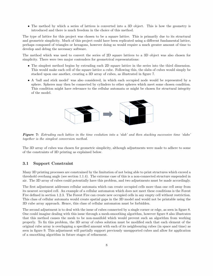
• The simplest method begins by extruding each 2D square lattice in the series into the third dimension.This would make each cell of the square lattice a cube. Following this, the slabs of cubes would simply bestacked upon one another, creating a 3D array of cubes, as illustrated in figure 7.

• A ‘ball and stick model’ was also considered, in which each occupied node would be represented by asphere. Spheres may then be connected by cylinders to other spheres which meet some chosen condition.This condition might have relevance to the cellular automata or might be chosen for structural integrityof the model.

Figure 7: Extruding each lattice in the time evolution into a ‘slab’ and then stacking successive time ‘slabs’together is the simplest conversion method.

The 3D array of cubes was chosen for geometric simplicity, although adjustments were made to adhere to someof the constraints of 3D printing as explained below.

3.1 Support Constraint

Many 3D printing processes are constrained by the limitation of not being able to print structures which exceed athreshold overhang angle (see section 1.1.4). The extreme case of this is a non-connected structure suspended inair. The 3D array of cubes could potentially have this problem, and two adjustments must be made accordingly.

The first adjustment addresses cellular automata which can create occupied cells more than one cell away fromits nearest occupied cell. An example of a cellular automaton which does not meet these conditions is the ForestFire defined in section 1.2.3. The Forest Fire can create new occupied cells in any empty cell without restriction.This class of cellular automata would create spatial gaps in the 3D model and would not be printable using the3D cube array approach. Hence, this class of cellular automaton must be forbidden.

The second adjustment is to deal with the issue of cubes connected by a single corner or edge, as seen in figure 8.One could imagine dealing with this issue through a mesh-smoothing algorithm, however figure 8 also illustratesthat this method causes the mesh to be non-manifold which would prevent such an algorithm from workingproperly. To fix this problem, the 3D array of cubes solution must be modified such that each element of theoriginal cube array is overlapping a specified amount with each of its neighbouring cubes (in space and time) asseen in figure 9. This adjustment will partially support previously unsupported cubes and allow for applicationof a smoothing algorithm in future stages of refinement.

8

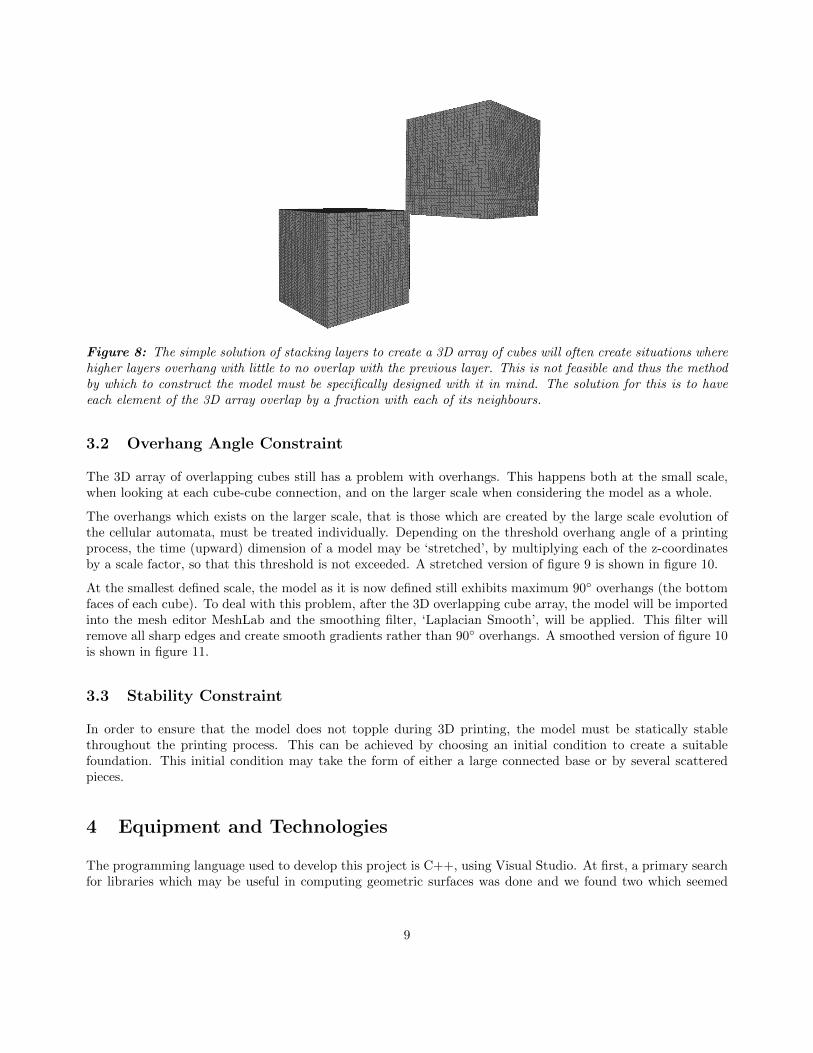
Figure 8: The simple solution of stacking layers to create a 3D array of cubes will often create situations wherehigher layers overhang with little to no overlap with the previous layer. This is not feasible and thus the methodby which to construct the model must be specifically designed with it in mind. The solution for this is to haveeach element of the 3D array overlap by a fraction with each of its neighbours.

3.2 Overhang Angle Constraint

The 3D array of overlapping cubes still has a problem with overhangs. This happens both at the small scale,when looking at each cube-cube connection, and on the larger scale when considering the model as a whole.

The overhangs which exists on the larger scale, that is those which are created by the large scale evolution ofthe cellular automata, must be treated individually. Depending on the threshold overhang angle of a printingprocess, the time (upward) dimension of a model may be ‘stretched’, by multiplying each of the z-coordinatesby a scale factor, so that this threshold is not exceeded. A stretched version of figure 9 is shown in figure 10.

At the smallest defined scale, the model as it is now defined still exhibits maximum 90◦ overhangs (the bottomfaces of each cube). To deal with this problem, after the 3D overlapping cube array, the model will be importedinto the mesh editor MeshLab and the smoothing filter, ‘Laplacian Smooth’, will be applied. This filter willremove all sharp edges and create smooth gradients rather than 90◦ overhangs. A smoothed version of figure 10is shown in figure 11.

3.3 Stability Constraint

In order to ensure that the model does not topple during 3D printing, the model must be statically stablethroughout the printing process. This can be achieved by choosing an initial condition to create a suitablefoundation. This initial condition may take the form of either a large connected base or by several scatteredpieces.

4 Equipment and Technologies

The programming language used to develop this project is C++, using Visual Studio. At first, a primary searchfor libraries which may be useful in computing geometric surfaces was done and we found two which seemed

9

Figure 9: In contrast to figure 8, these two cubes are overlapping by half in each dimension. This fixes theproblem of cubes sharing only an edge or corner.

Figure 10: In order to control the overall large scale angle of the geometry the model may be stretched in thetime (z) dimension.

promising, namely CGAL [21] and VCG [22]. However, after tinkering with these libraries, it was clear thatthey provided far too much depth for this project and would be far too complex to apply to such a simpleproblem. Hence, it was decided to develop our own mini-library from the ground up with our specific needs inmind. In developing the GUI (see section 5.3), the QT and Boost libraries for C++ were used for frame andwidget manipulation.

MeshLab [23] was used as the primary software to view triangulated surfaces produced by the project code. Itwas also a most important tool in smoothing our triangulated 3D polyhedrons which was composed of discretecubes into more continuous and less ‘cube-y’ polyhedrons.

In order to prepare 3D models for printing, NetFabb (a STL file repair and modification tool) [24] was used tocorrect any syntactical faults in our smoothed STL files. NetFabb was also used to resize and set the units ofour model to ensure the correct model dimensions before printing.

A RepRap 3D-printer [25] was used to bring our triangulated model to physical realisation. A software knownas Slic3r [26] was used to convert print-ready STL files into instructions for the movement of the printer nozzle,known as GCode.

10

Figure 11: To deal with the inevitable issue of small scale overhangs in a cube model, up to three iterations ofa ‘Laplacian Smoothing’ function were applied from MeshLab.

5 Description of Software Developed

A basic description of the purpose of the code written is found below, however if more detailed knowledge isdesired the source code can be found open-source by navigating to the url in [27].

The software developed for this project is composed in three main sections. The first section is a set of classeswhich incorporate the properties of the square lattice and enables a user to easily define the rules of a cellularautomaton and the initial conditions of the lattice, described in section 5.1. The second section is a set of classeswhich allows the user to take a set of lattices and transform them into a 3D triangulated polyhedron, describedin section 5.2. The last main section is a GUI which allows the users to easily set parameters, visualize thecellular automata, and create 3D polyhedrons without editing the source code, described in section 5.3.

5.1 Lattice and Iterative Model Structures

The purpose of the first main section of the software is to evolve a cellular automaton, defined on a squarelattice, through a number of iterations. This is accomplished through two classes: Lattice which defines thelattice of cells, and Model which defines the set of rules by which the lattice evolves.

The Lattice type was defined in such a way that any cell of the lattice would easily be able to access any ofits neighbours, as cellular automaton very commonly evolve through neighbour-neighbour interactions. This isespecially important for the cellular automata which concern this project, namely those which do not createoccupied cells more than one cell away from the nearest occupied cell.

To effectively link all cells to their neighbours, the Lattice type is defined as a square array of LatElem, a simpletype which stores the state of the cell, as well as pointers to each of its eight neighbouring LatElem (those whichshare at least one vertex). The state of each element is an enumerated type, which allows for easy modificationof allowable states if a cellular automaton requires more than empty and occupied states.

Model is defined as a super-class to allow for many types of cellular automata to inherit generic properties whileeach having their own set of rules. The Model type takes an initial Lattice and stores it. Each derived class hasan iterate function where the user may define how the cellular automaton evolves. When this function is called,Model stores the result as the current Lattice. Hence by iterating the model several times a series of Lattice isstored, capturing the cellular automaton’s evolution.

11

5.2 Lattice to Polyhedron Conversion

The next major section of development was conversion from a series of Lattice, stored in a Model, into a 3Dpolyhedron, composed of cubes. This conversion is split into two important processes. The first process isconverting the series of Lattice into a 3D CubeArray, a type which overlaps the lattice cells to overcome theobstacle of two neighbouring cubes being connected by a single edge. The second process is converting theCubeArray into a triangulated Polyhedron, a type which stores the vertex and face information of a polyhedronand has the ability to export this information in a variety of formats.

The CubeArray type allows the user to define the fraction by which each cell of each Lattice in the series overlapswith its neighbours in both space and time. To emulate overlapping the lattice cells the CubeArray is definedas a 3D array of the appropriate size (depending on the amount of defined overlap between LatElem). Theelements of a CubeArray are CubeElem, and each represent several overlapping fractional lattice cells. EachCubeElem stores the state (empty or occupied) and points to its six neighbouring CubeElem with which it sharesa face.

The algorithm to fill a CubeArray from a series of Lattice is relatively straight forward. First the CubeArray isdefined at the appropriate size and initialized to be completely empty. The computer determines which CubeElemcorrespond to the occupied LatElem and changes the state of those CubeElem to full. This accomplishes bothfusing the several lattice layers into one object and overlapping each cell with its neighbours.

Next, the CubeArray must be converted into a Polyhedron, a type which stores vertex and face informationabout a 3D polyhedron. However, we do not want the Polyhedron to store information about the faces of theCubeArray which are not on the surface of the entire object. The Polyhedron type is a list of 3-vectors describingthe position of the object’s vertices, and a list of faces. Each face is defined by a list of indices, which referencethe vertices of the Polyhedron. The normal vector of the face is defined by the order of the vertex indices withinthe face, in a right handed fashion.

When the Polyhedron is created, it iterates over the CubeArray searching for occupied cubes. When an occupiedcube is found, the computer checks for any shared faces between the cube and its neighbours. It then storesthe information of faces which are not shared between two cubes as these faces must be on the surface of theobject. The Polyhedron type has the capability of exporting this information in either the .stl or the .ply filetype, described in section 1.1.6, for rendering in a mesh viewer and later for smoothing and printing.

5.3 GUI Elements

A GUI was developed with two main purposes in mind. The first purpose is to allow the user to more easilychange parameters of the cellular automaton. Such parameters might include lattice size or statistical elements.This removes the large burden on the user of having to edit the source code each time to run a slightly differentsimulation. Examples of options users have before running the simulation can be seen in figure 12.

The second purpose is to allow visualization of the cellular automaton in real time as well as allowing the userto easily choose the initial conditions of the simulation, as illustrated in figure 13. This could be especiallyuseful in helping the user determine when to stop iterating the cellular automaton and export the 3D model.This could also be interesting when comparing the animated 2D evolution to the 3D model.

6 Achievements and Results

Although the software described in section 5 could be used to simulate any cellular automata, two cellularautomata which meet the constraints mentioned in section 3 were chosen to demonstrate its capabilities.

12

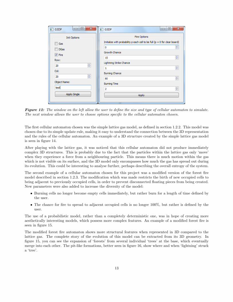
Figure 12: The window on the left allow the user to define the size and type of cellular automaton to simulate.The next window allows the user to choose options specific to the cellular automaton chosen.

The first cellular automaton chosen was the simple lattice gas model, as defined in section 1.2.2. This model waschosen due to its simple update rule, making it easy to understand the connection between the 3D representationand the rules of the cellular automaton. An example of a 3D structure created by the simple lattice gas modelis seen in figure 14.

After playing with the lattice gas, it was noticed that this cellular automaton did not produce immediatelycomplex 3D structures. This is probably due to the fact that the particles within the lattice gas only ‘move’when they experience a force from a neighbouring particle. This means there is much motion within the gaswhich is not visible on its surface, and the 3D model only encompasses how much the gas has spread out duringits evolution. This could be interesting to analyse further, perhaps describing the overall entropy of the system.

The second example of a cellular automaton chosen for this project was a modified version of the forest firemodel described in section 1.2.3. The modification which was made restricts the birth of new occupied cells tobeing adjacent to previously occupied cells, in order to prevent disconnected floating pieces from being created.New parameters were also added to increase the diversity of the model:

• Burning cells no longer become empty cells immediately, but rather burn for a length of time defined bythe user.

• The chance for fire to spread to adjacent occupied cells is no longer 100%, but rather is defined by theuser.

The use of a probabilistic model, rather than a completely deterministic one, was in hope of creating moreaesthetically interesting models, which possess more complex features. An example of a modified forest fire isseen in figure 15.

The modified forest fire automaton shows more structural features when represented in 3D compared to thelattice gas. The complete story of the evolution of this model can be extracted from its 3D geometry. Infigure 15, you can see the expansion of ‘forests’ from several individual ‘trees’ at the base, which eventuallymerge into each other. The pit-like formations, better seen in figure 16, show where and when ‘lightning’ strucka ‘tree’.

13

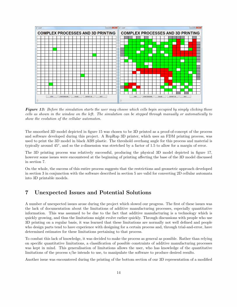
Figure 13: Before the simulation starts the user may choose which cells begin occupied by simply clicking thosecells as shown in the window on the left. The simulation can be stepped through manually or automatically toshow the evolution of the cellular automaton.

The smoothed 3D model depicted in figure 15 was chosen to be 3D printed as a proof-of-concept of the processand software developed during this project. A RepRap 3D printer, which uses an FDM printing process, wasused to print the 3D model in black ABS plastic. The threshold overhang angle for this process and material istypically around 45◦, and so the z-dimension was stretched by a factor of 1.5 to allow for a margin of error.

The 3D printing process was relatively successful, producing the physical 3D model depicted in figure 17,however some issues were encountered at the beginning of printing affecting the base of the 3D model discussedin section 7.

On the whole, the success of this entire process suggests that the restrictions and geometric approach developedin section 3 in conjunction with the software described in section 5 are valid for converting 2D cellular automatainto 3D printable models.

7 Unexpected Issues and Potential Solutions

A number of unexpected issues arose during the project which slowed our progress. The first of these issues wasthe lack of documentation about the limitations of additive manufacturing processes, especially quantitativeinformation. This was assumed to be due to the fact that additive manufacturing is a technology which isquickly growing, and thus the limitations might evolve rather quickly. Through discussions with people who use3D printing on a regular basis, it was learned that these limitations are normally not well defined and peoplewho design parts tend to have experience with designing for a certain process and, through trial-and-error, havedetermined estimates for these limitations pertaining to that process.

To combat this lack of knowledge, it was decided to make the process as general as possible. Rather than relyingon specific quantitative limitations, a classification of possible constraints of additive manufacturing processeswas kept in mind. This generalisation of limitations allows the user, who has knowledge of the quantitativelimitations of the process s/he intends to use, to manipulate the software to produce desired results.

Another issue was encountered during the printing of the bottom section of our 3D representation of a modified

14

Figure 14: An example of a 2D lattice gas expanding in time. On the left is the direct output of the codewritten for this project, the overlapping array of cubes. On the right is the same model after smoothing. Bothfigures were rendered in MeshLab [23].

Figure 15: Rough and smooth representation of the modified forest fire model updating itself in time.

forest fire, due to our lack of experience with 3D printers. Early in the FDM printing process, the extrusionnozzle came into contact with the base of the model. This caused the motor to skip and caused what hadalready been printed to become offset, as seen in figure 18.

The string-like structures, seen in sections of the underside of the model in figure 18, is what happens when theFDM process attempts to print with no supporting structure, a direct result of the offset of the upper-sectionrelative to the base.

It was suggested that the reason for the nozzle hitting the base was that some of the structures in our modelwere too thin. The thin structures may have curled upwards significantly when cooling, putting them in theway of the unknowing extrusion nozzle. Further, people familiar with the Reprap printer suggested that theremay be an easy fix for this by changing some of the printer’s settings, namely the temperatures of the bed orextrusion head or possibly the speed of the extrusion nozzle. With more time, it may have been possible toexperiment with settings to create a flawless print.

8 Extensions and Future Work

In the future it would be possible to use the tool we have created here to explore the parameter space of desiredcellular automata. Different parameters could lead to obvious features in three dimensions which were not clearfrom their 2D evolution alone. Classifying different emergent 3D features by the parameter space could be useful

15

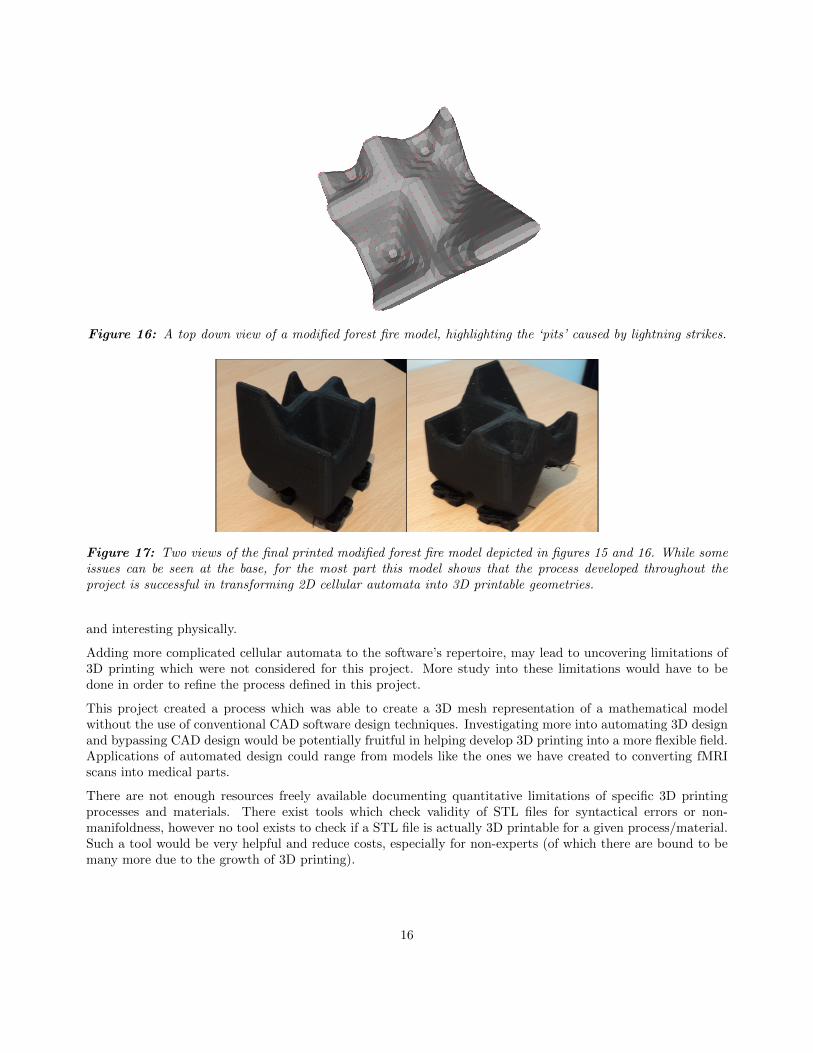
Figure 16: A top down view of a modified forest fire model, highlighting the ‘pits’ caused by lightning strikes.

Figure 17: Two views of the final printed modified forest fire model depicted in figures 15 and 16. While someissues can be seen at the base, for the most part this model shows that the process developed throughout theproject is successful in transforming 2D cellular automata into 3D printable geometries.

and interesting physically.

Adding more complicated cellular automata to the software’s repertoire, may lead to uncovering limitations of3D printing which were not considered for this project. More study into these limitations would have to bedone in order to refine the process defined in this project.

This project created a process which was able to create a 3D mesh representation of a mathematical modelwithout the use of conventional CAD software design techniques. Investigating more into automating 3D designand bypassing CAD design would be potentially fruitful in helping develop 3D printing into a more flexible field.Applications of automated design could range from models like the ones we have created to converting fMRIscans into medical parts.

There are not enough resources freely available documenting quantitative limitations of specific 3D printingprocesses and materials. There exist tools which check validity of STL files for syntactical errors or non-manifoldness, however no tool exists to check if a STL file is actually 3D printable for a given process/material.Such a tool would be very helpful and reduce costs, especially for non-experts (of which there are bound to bemany more due to the growth of 3D printing).

16

Figure 18: The underside of the printed model shows that, early in the printing process, the nozzle becameoffset from the base it had already printed.

9 Conclusion

With the rapid growth of the 3D printing industry, it only seems natural to try to take advantage of thisrevolutionary manufacturing technology in every way possible. Representing physical processes in 3D by aphysical object could be interesting to physicists and non-physicists alike. It allows for possible further insightinto the process which may have been elusive in 2D or could perhaps add to the growing collections of 3Dprinted art around the world.

This project was mostly successful in meeting its objectives. A process by which to convert a 2D cellularautomaton into a 3D printable object was developed. The limitations of the different additive manufacturingtechnologies were generalised and taken into account while developing the process. A software was designed toautomate the process and allow a user to easily transform a cellular automaton into a 3D object.

Hopefully more developments will be made within the physics community which take advantage of the evolving3D printing technology. As 3D printing technology evolves further it could help to develop representationsand aid visualisation, similar to what was done in this project, or to create customized parts for experimentsat a reduced cost. In any case, the physics community can only benefit by taking part in this technologicalrevolution.

References

[1] Ian Gibson, David Rosen, and Brent Stucker. Additive Manufacturing Technologies. Springer, 2010.

[2] TRowe Price. A brief history of 3d printing infographic. http://individual.troweprice.com/

staticFiles/Retail/Shared/PDFs/3D_Printing_Infographic_FINAL.pdf, December 2011.

[3] Justin Scott. Additive manufacturing: Status and opportunities. Technical report, IDA Science andTechnology Policy Institute, 2012.

[4] Scott Crump. Direct digital manufacturing. Technical report, Fortus 3D Production Systems, 2009. http://files.asme.org/MEMagazine/PaperLibrary/30064.pdf.

[5] 3D Printshow Homepage. http://www.3Dprintshow.com/, March 2013.

17

[6] Tim Evans. Project proposal: Complex processes and 3d printing. https://workspace.imperial.ac.uk/physicsuglabs/Public/3rd_Year_Projects/Projects%202012-13/Computational/Evans1.pdf, Octo-ber 2012.

[7] eFundaINC. Fused deposition modeling. http://www.efunda.com/processes/rapid_prototyping/fdm.cfm, 2013.

[8] D. T. Pham and S. S. Dimov. Rapid Manufacturing. Springer-Verlag, 2001. Image of FDM Process.

[9] U. of Texas Mechanical Engineering Department. Selective laser sintering, birth of an industry. http:

//www.me.utexas.edu/news/2012/0712_sls_history.php#ch4, December 2012.

[10] Fred Fischer. Thermoplastics: The best choice for 3d printing. http://www.stratasys.com/resources/

~/media/Main/Secure/White%20Papers/Rebranded/SSYS-WP-Thermoplastics-03-13.ashx, 2011.

[11] et al. R. Liska, M.Schuster. Photopolymers for rapid prototyping. J. Coat. Technol. Res., 2007.

[12] J. Kruth, M. Leu, and T. Nakagawa. Progress in additive manufacturing and rapid prototyping. CIRPAnnals - Manufacturing Technology, 1998.

[13] 3D Printing Era. Overhang threshold image. http://www.3dprintingera.com/

3d-printing-overhangs-and-bridges/, March 2013.

[14] R Hauge, I Campbell, and P Dickens. Implications on design of rapid manufacturing. Journal of MechanicalEngineering Science, 2003.

[15] Kaufui Wong and Aldo Hernandez. A review of additive manufacturing. ISRN Mechanical Engineering,2012.

[16] Shapeways. Things to keep in mind when desiging for 3d printing. http://www.shapeways.com/

tutorials/things-to-keep-in-mind, February 2013.

[17] Stephen Wolfram. Universality and complexity in cellular automata. Physica D, January 1984.

[18] J Coe, S Ahnert, and T Fink. When are cellular automata random? In Theory of Condensed Matter,Cavendish Laboratory. 2008.

[19] Stephen Wolfram. Cellular automata as models of complexity. Nature, October 1984.

[20] Henrik Jeldtoft Jensen. Self-Organized Criticality. Cambridge University Press, 1998.

[21] CGAL Development Team. Computational geometry algorithms library. http://www.cgal.org/, February2013.

[22] Visual Computing Lab. Visualization and computer graphics library. http://vcg.isti.cnr.it/

~cignoni/newvcglib/html/, February 2013.

[23] 3D-Coform Consortium. Meshlab. http://meshlab.sourceforge.net/, February 2013.

[24] NetFabb. http://www.netfabb.com/, March 2013.

[25] RepRap Wiki. http://www.reprap.org/wiki/Main_Page, March 2013.

[26] Alessandro Ranellucci. Slic3r website. http://www.slic3r.org/about, March 2013.

[27] Dominic Reiss and Joshua Price. Complex processes and 3d printing source code. https://github.com/

doreiss/3D_Print, May 2013.

18