Int J Fract (2019) 215:1–37https://doi.org/10.1007/s10704-018-0324-5

ORIGINAL PAPER

Complete analytical solutions for double cantilever beamspecimens with bi-linear quasi-brittle and brittle interfaces

Leo Škec · Giulio Alfano · Gordan Jelenic

Received: 21 February 2018 / Accepted: 24 October 2018 / Published online: 14 November 2018© The Author(s) 2018

Abstract In this workwe develop a complete analyti-cal solution for a double cantilever beam (DCB) wherethe arms are modelled as Timoshenko beams, and abi-linear cohesive-zone model (CZM) is embedded atthe interface. The solution is given for two types ofDCB; one with prescribed rotations (with steady-statecrack propagation) and one with prescribed displace-ment (where the crack propagation is not steady state).Because the CZM is bi-linear, the analytical solutionsare given separately in three phases, namely (i) linear-elastic behaviour before crack propagation, (ii) damagegrowth before crack propagation and (iii) crack prop-agation. These solutions are then used to derive thesolutions for the casewhen the interface is linear-elasticwith brittle failure (i.e. no damage growth before crackpropagation) and the case with infinitely stiff interfacewith brittle failure (corresponding to linear-elastic frac-ture mechanics (LEFM) solutions). If the DCB armsare shear-deformable, our solution correctly capturesthe fact that they will rotate at the crack tip and in front

L. Škec (B) · G. AlfanoDepartment of Mechanical and Aerospace Engineering,Brunel University London, Kingston Lane,Uxbridge UB8 3PH, UKe-mail: leo.skec@brunel.ac.uk

G. Alfanoe-mail: giulio.alfano@brunel.ac.uk

G. JelenicFaculty of Civil Engineering, University of Rijeka,Radmile Matejcic 3, Rijeka 51000, Croatiae-mail: gordan.jelenic@uniri.hr

of it even if the interface is infinitely stiff. Expressionsdefining the distribution of contact tractions at the inter-face, as well as shear forces, bending moments andcross-sectional rotations of the arms, at and in frontof the crack tip, are derived for a linear-elastic inter-face with brittle failure and in the LEFM limit. For aDCB with prescribed displacement in the LEFM limitwe also derive a closed-form expression for the crit-ical energy release rate, Gc. This formula, comparedto the so-called ‘standard beam theory’ formula basedon the assumptions that the DCB arms are clamped atthe crack tip (and also used in standards for determin-ing fracture toughness in mode-I delamination), has anadditional term which takes into account the rotationat the crack tip. Additionally, we provide all the men-tioned analytical solutions for the case when the shearstiffness of the arms is infinitely high, which corre-sponds to Euler–Bernoulli beam theory. In the numer-ical examples we compare results for Euler–Beronulliand Timoshenko beam theory and analyse the influenceof the CZM parameters.

Keywords DCB test · Mode-I delamination ·Analytical solution · Timoshenko beam theory ·Cohesive-zone model · Linear-elastic fracturemechanics

123

2 L. Škec et al.

List of symbols

A Cross-sectional area of a single DCB arma Crack lengtha0 Initial crack lengthb Width of a DCBCi Integration constants for the undamaged

part (i = 1, . . . , 6)C ji Constants depending on C3, C4, ξ3 and ξ4

(i = 3, 4 and j = M, T )Ci Integration constants for the undamaged

part that are zero because of the bound-ary conditions for a semi-infinite DCB (i =1, . . . , 6)

c2 function cos(Lczκξ2)

c2 function cos(Lczκξ2)

ch1 function cosh(Lczκξ1)

ch1 function cosh(Lczκξ1)

D Dirac deltaD0 A constant depending on ψ

Di Integration constants for the damaged part(i = 1, . . . , 4)

Di j Constants for the damaged part dependingon the value of ω (i = 1, . . . , 4 and j =1, 2)

E Young’s modulus of DCB armsF Vertical force applied on the upper layer of

a DCB with prescribed displacementF0 A tensile stress resultant (concentrated

force) at the crack tip for the LEFM limitcase

FE Value of the applied force computed usingEuler–Bernoulli beam theory

FL Maximum value of the applied force in thelinear-elastic phase for a DCB with pre-scribed displacement

Fmax Maximum value of the applied load for aDCB with prescribed displacement

FT Value of the applied force computed usingTimoshenko beam theory

Fσmax Value of the applied force computed for afinite value of σmax

F∞ Value of the applied force for the LEFMlimit

Gc Critical energy release rateH Heaviside functionh Depth of a single DCB armI Secondmoment of area of the cross-section

of a single DCB arm

Jc Critical value of the J integralks Shear correction coefficientL Total length of a DCB specimenLcz Length of the cohesive or damage-process

zoneLcz Maximum value of Lcz for a DCBwith pre-

scribed rotationsLmaxcz Maximum value of Lcz for a DCBwith pre-

scribed displacementLmincz Minimum value of Lcz during crack propa-

gation for a DCB with prescribed displace-ment

M Concentrated moment applied on a DCBarm

M1 Bending moment in the upper DCB arm onthe part where the interface is undamaged

ML1 LEFM limit value of M1

M2 Bending moment in the upper DCB arm onthe part where the interface is damaged

ML Maximum value of the applied moment inthe linear-elastic phase

Mmax Maximum value of the applied momentq Distributed transverse loading along the

upper DCB armri Roots of the characteristic equation for the

undamaged part (i = 1, . . . , 4)s2 function sin(Lczκξ2)

s2 function sin(Lczκξ2)

sh1 function sinh(Lczκξ1)

sh1 function sinh(Lczκξ1)

T Shear force in the upper DCB armT1 Shear force in the upper DCB arm on the

part where the interface is undamagedT L1 LEFM limit value of T1

T2 Shear force in the upper DCB arm on thepart where the interface is damaged

ti Roots of the characteristic equation for thedamaged part (i = 1, . . . , 4)

v Transversal displacement of the upper DCBarm

v1 Transversal displacement of the upper DCBarm on the part where the interface isundamaged

vL1 LEFM limit value of v1

v2 Transversal displacement of the upper DCBarm on the part where the interface is dam-aged

x Co-ordinate along the interface

123

Complete analytical solutions for double cantilever beam 3

x0 Co-ordinate x corresponding to zero stressat the interface for the case of a linear-elasticinterface with brittle failure

xmin Co-ordinate x corresponding to the mini-mum (maximum compressive) stress at theinterface for the case of a linear-elasticinterface with brittle failure

α A constant defined as α = δ0/δcβi Constants depending on ξ j , Dkl , κ and a0

(i = 1, . . . , 8, j = 1, 2, k = 1, . . . , 4 andl = 1, 2)

γ Shear strain in the upper DCB arm� Prescribed crack mouth opening displace-

ment of a DCB�a Part of the crack mouth opening displace-

ment due to bending of the arms assumingthat they are clamped at the crack tip

�δCT Part of the crack mouth opening displace-

ment due to the opening at the crack tip�

ϕCT Part of the crack mouth opening displace-

ment due to the rotation at the crack tipδ Relative displacement at the interface in

mode Iδ0 Linear-elastic limit value of the relative dis-

placement at the interface in mode Iδc Relative displacement at the interface corre-

sponding to the total loss of interconnectionin mode I

εr Relative error due to using Euler–Bernoulliinstead of Timoshenko beam theory

εr Relative difference between CCM andLEFM solutions

ζi Constants depending on ω (i = 1, . . . , 4)ζ i Constants depending on ω (i = 1, . . . , 4)η A constant defined as η = λ/κ

ηE A constant defined as ηE = λE/κ

θ Prescribed rotation on a DCB armκ A constant depending on the bending stiff-

ness of DCB arms and the softening partof the σ − δ traction-separation law of theinterface

λ A constant depending on the bending stiff-ness of DCB arms and the linear-elasticstiffness of the interface

λE A constant defined as λE = √2λ/2

μ Shear modulus of DCB armsν Poisson’s ratio of DCB armsξi Constants depending on ψ (i = 1, 2)ρi Constants defined as ρi = ζi/λ (i = 1, 2)

σ Contact traction at the interface in mode Iσ L LEFM limit value of σ

σmax Maximum value of contact tractions at theinterface in mode I

ϕ Cross-sectional rotation of the upper DCBarm

ϕ1 Cross-sectional rotation of the upper DCBarm on the part where the interface isundamaged

ϕ2 Cross-sectional rotation of the upper DCBarm on the part where the interface is dam-aged

ϕL1 LEFM limit value of ϕ1

χ A constant defined as χ = E I/(2μAs)

ψ A constant depending on bending and shearstiffness of DCB arms, and κ

ω A constant depending on bending and shearstiffness of DCB arms, and λ

List of Abbreviations

ASTM American Society for Testing andMaterialsBS British StandardCBBM Compliance-based beam methodCBT Corrected beam theoryCCM Cohesive crack modelCZM Cohesive zone modelDCB Double cantilever beamEBT Enhanced beam theoryESBT Enhanced simple beam theoryFE Finite elementFEA Finite element analysisISO International Organization for Standardiza-

tionLEFM Linear elastic fracture mechanicsSBT Simple beam theoryTDCB Tapered double cantilever beam

1 Introduction

Since introduced in 1960s by Dugdale (1960) andBarenblatt (1959), the use of cohesive-zone models(CZM) has become one of the most popular ways ofdescribing fracture processes within the research com-munity (Hillerborg et al. 1976; Alfano and Crisfield2001; Park and Paulino 2011). Nowadays CZMs arewidely implemented within the framework of finite-element analysis (FEA) and interface elements, based

123

4 L. Škec et al.

on CZMs, can be found in element libraries of manycommercial softwares for FEA used to solve delamina-tion/debonding problems in 2D (Alfano and Crisfield2001) and 3D (Park and Paulino 2011). However,because the accuracy of such computations is alwaysdependent on the size of the FEmesh, they can be com-putationally demanding and suffer from convergenceproblems.

One of the ways to reduce the computational costof the analysis was already proposed by the first andthird author and consists of using beam finite elementsinstead of plane solids to model the bulk material of thespecimens in 2D analysis of delamination. The resultswere presented for single-mode (I and II) and mixed-mode delamination problems in geometrically linear(Škec et al. 2015) and non-linear analysis (Škec andJelenic 2017). Compared to models which use planesolid FEs, the computational efficiency of the beammodel was improved (the reduction of total number ofdegrees of freedom can go up to 40%) without any sig-nificant loss in the accuracy. However, the beammodelstill suffered from convergence problems and spuriousoscillations around the exact solution for cases of brit-tle interfaces when the mesh is not sufficiently refined.For this reason, it is always very useful when an analyt-ical or semi-analytical solution can be found for casesof engineering interest.

In this paper we focus on mode-I delamination andthe double cantilever beam (DCB) test, which is thestandard test for determining fracture toughness inmode I. We use quasi-static and geometrically linearanalysis where the arms of the DCB are modelled asTimoshenko beams and at the interface, a bi-linearCZM is used. Since the traction–separation law at theinterface is composed of two linear parts and a final partwith zero tractions, the solution of the problem can beobtained analytically, separately for each part of theinterface whose state falls within one of the linear partsof the traction separation law. Because all the quantitiesof the problem will be expressed exactly with no needfor discretisation, the computational cost is negligibleand the obtained solutions have no spurious oscilla-tions, which typically occur when delamination prob-lems are solved using FE analysis (Alfano andCrisfield2001; Blackman et al. 2003b; Škec et al. 2015). How-ever, the idea of using analytical solutions for a DCB isnot new and many researchers have contributed to thefield in the last 50 years.

The simplest way to analytically model a DCBwould be to assume that the arms of the specimenact as if they were cantilever beams clamped at thecrack tip. Under this assumption, Benbow and Roesler(1957) used Euler–Bernoulli beam theory to establishthe Griffith’s energy balance for a flat-strip specimenwhere the crack gradually propagates down the middleby holding the specimen in a state of lengthwise com-pression. During 1960s and early 1970s, Ripling et al.(1971) introduced the DCB and tapered double can-tilever beam (TDCB) tests and specimens. They alsoprovided analytical formulae based on Irwin’s energyapproach (Irwin 1956) and Timoshenko beam theory(assuming that the arms are clamped at the crack tip) tocompute the fracture toughness of the adhesive, whichin 1974 becamepart of theAmerican standard for deter-mining fracture toughness of adhesive joints in modeI. The current version of that standard, ASTM D3433-99 (reapproved in 2012) (ASTMD3433-99 2012), stillexclusively uses the same formulae proposed inRiplinget al. (1971). The formula for the DCB used in ASTMD3433-99 (2012) is also used in BS ISO 25217:2009(2009), where it is called ‘simple beam theory’ (SBT).Wewill adopt this terminology and use the term ‘simplebeam theory’ (SBT) for formulations based on simplebeam theories (Euler–Bernoulli or Timoshenko) andthe assumption that the DCB arms act as if they wereclamped at the crack tip.

However, Ripling et al. (1971) noticed that the SBTformula gives smaller deflections than those obtainedfrom the experiments and they attributed it to not takinginto account the rotations of the arms which take placeat the crack tip. They also suggested that the resultscould be simply corrected by increasing the measuredcrack length by a fixed amount. Although they did notpropose amethod to obtain this crack length correction,this concept was further developed by other researchers(Blackman et al. 2003a) and became the basis for adata reduction scheme in BS ISO 25217:2009 (2009)called ‘corrected beam theory’ (CBT) based on Euler–Bernoulli beam theory. de Moura et al. (2008) devel-oped the so-called ‘compliance-based beam method’(CBBM) where the corrected-crack-length conceptwas used with Timoshenko beam theory.

Kanninen (1973) presented an analytical model fora DCB where the upper arm was modelled as a Euler–Bernoulli beam on elastic foundation (Winkler model),allowing for relative displacements and rotations at thecrack tip and ahead of it. The very next year (Kan-

123

Complete analytical solutions for double cantilever beam 5

ninen 1974) extended his formulation to account forthe shear deformability of the arms and rotational stiff-ness of the interface, which was accomplished by usingTimoshenko beam theory and Pasternak elastic foun-dation. However, Gehlen et al. (1979) (with Kanninenas the third author) showed that the rotational stiffnessof the foundation springs is not relevant in a symmet-rical DCB configuration. Kanninen’s model (Kanni-nen 1974) was later extended by Williams (1989) toaccount for orthotropic material behaviour. Shahaniand Forqani (2004), Shahani and Amini Fasakhodi(2010) developed solutions for a DCB model of finitelength consisting of a Timoshenko beam lying on anelastic Winkler foundation for the conditions of fixedforce and fixed displacement. Most of the mentionedpapers (Kanninen 1973, 1974; Gehlen et al. 1979; Sha-hani and Forqani 2004; Shahani and Amini Fasakhodi2010) also investigate the dynamic analysis of unsta-ble crack propagation and arrest in a DCB test. We willrefer to the beam-on-elastic-foundation DCB modelsas ‘enhanced beam theory’ (EBT) models.

In EBTmodels the interface acts elastically linear upto a certain point where brittle failure occurs. However,fracture processes can usually introduce a certain levelof quasi-brittle behaviour, which cannot be capturedusing EBT models. It is, however, well know that thequasi-brittle behaviour of the interface in a DCB testhas an important influence on the structural responsebefore the crack starts to propagate, whereas during thecrack propagation the influence of the interface ductil-ity is negligible. One way of introducing a quasi-brittlebehaviour of the interface in the model is to use CZMswhich account for progressive softening/damage aftera certain critical value of the traction at the interfacehas been reached.

Stigh (1988) developed an analytical solution for aDCB where the arms are modelled as Euler–Bernoullibeams and a bi-linear CZM is embedded at the inter-face. This solution was revisited and extended toaccount for a finite length of the specimen and a trape-zoidal CZM by Dimitri et al. (2017). de Morais (2013)proposed a solution for aDCBwith prescribed rotations(loaded with moments) where the arms are modelledas Timoshenko beams and a bi-linear CZM is embed-ded at the interface. Unlike Williams (1989) who gavethe complete solution for the linear-elastic phase of theinterface behaviour, deMorais (2013) took into accountonly real roots of the characteristic equation of the dif-ferential equation of the problem.We discuss this issue

in detail in Sect. 2.2. We will refer to the models withquasi-brittle crack as ‘cohesive crack models’ (CCM)(Dimitri et al. 2017).

To the best of authors’ knowledge, a complete ana-lytical solution for a DCB with arms modelled as Tim-oshenko beams and the interface modelled using a bi-linear CZM, which covers any of the two cases of pre-scribed rotations and displacement, is not available inthe literature. Therefore, one aim of this paper is to fillthis gap and to show a clear relationship between SBT,EBT and CCM solutions for a DCB for both Euler–Bernoulli and Timoshenko beam theory.

Furthermore, reducing the general CCM solutiondown to the SBT solution shows that even in the limitcase of LEFM, rotations at the crack tip and in frontof it still occur when Timoshenko beam theory is used.Thus, the assumption made in SBT that the arms actas if they were clamped at the crack tip is not appli-cable even for an infinitely stiff perfectly brittle inter-face, which is assumed in LEFM. This is somehowan expected result since even an infinitely stiff inter-face cannot prevent the bulk material of the arms todeform (rotate) around the interface. However, the factthat we can capture this behaviour using Timoshenkobeam theory, to the best of authors’ knowledge, hasnot been addressed in the literature so far. More gen-erally, a comprehensive investigation of the analyticalsolutions for the LEFM limit is lacking in the litera-ture. Thus, we call this novel approach ‘enhanced sim-ple beam theory’ (ESBT). However, we will show thatwhen the shear deformability of the arms is excludedfrom the model, which corresponds to Euler–Bernoullibeam theory, ESBT is equivalent to SBT. A second aimof this paper is to determine the interface stresses andthe stress resultant profiles in the LEFM cases. We willalso show that a novel LEFM-based formula for thedetermination of the critical energy release rate, Gc,can be derived. This formula takes into account therotation at the crack tip, unlike those currently avail-able in the standards (ASTM D3433-99 2012; BS ISO25217:2009 2009).

The outline of the paper is as follows. In Sect. 2, wedefine the problem and derive the general solutions ofdifferential equations of the problem. In Sects. 3 and4, we determine the integration constants for the casesof DCB with prescribed rotations and DCB with pre-scribed displacement, respectively. The solutions aregiven in a unified and compact form, thus avoiding

123

6 L. Škec et al.

cumbersome expressions which can be often encoun-tered in such analytical solutions.

The presented general CCM solutions (based onTimoshenko beam theory and a bi-linear CZM at theinterface) are then used to derive solutions for dif-ferent particular cases. EBT solutions presented inSect. 5 are obtained from CCM solutions by makingthe interface brittle (removing the softening branch inthe traction–separation law of the interface), whereasESBT (LEFM-based) solutions presented in Sect. 6are obtained from EBT solutions by letting the inter-face stiffness go to infinity. The solutions for Euler–Bernoulli beam theory (including CCM, EBT and SBTsolutions) given in “Appendix B” are obtained from theTimoshenko beam theory solutions by letting the shearstiffness become infinite.

Results obtained by means of the presented ana-lytical solutions are studied for a number of cases,including sensitivity analyses on the interface strength.In particular, results for a linear interface with brittlebehaviour and in the LEFM limit are presented anddiscussed in Sect. 7.3.

2 Problem description

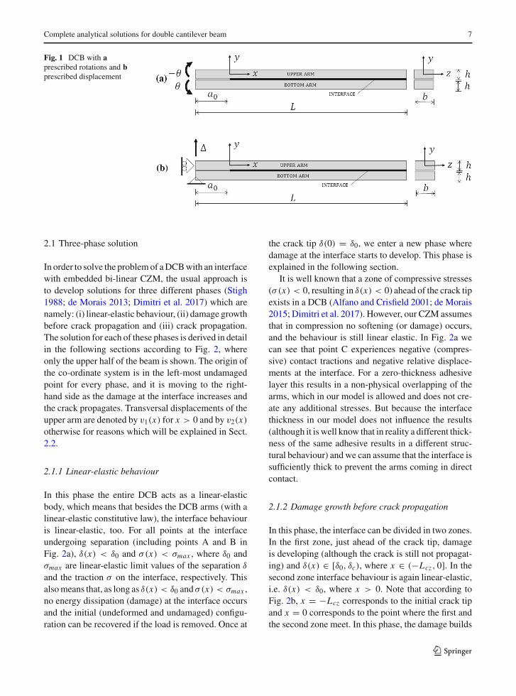
Consider a double cantilever beam (DCB) of length Lcomposed of two identical arms with depth h, width band the initial crack length a0, as shown in Fig. 1. Eacharm is modelled as a Timoshenko beam with a linear-elastic constitutive law, where material properties aredefined by Young’s modulus, E , and shear modulus,μ.In a general case E and μ can have independent val-ues, while for an isotropic material μ = 0.5E/(1+ ν),where ν is Poisson’s ratio. Mode-I problem is con-sidered, so that loads are applied symmetrically withrespect to the mid-plane of the interface between thetwo arms. Therefore, stresses and strains in a DCB aresymmetrical with respect to the mid-plane of the inter-face, which means that, for the sake of simplicity, onlyone armcan be considered in the analysis. In the presentpaper we will consider only the upper arm and assumethat the x-axis is the centroidal axis of the arm (refer-ence axis), while y and z axes are the principal axes ofthe arm’s cross section (see Fig. 1).

In our approach, Timoshenko beam theory is usedto model the DCB arms, which implies that we assumethat displacements and rotations of the arms are rel-atively small compared to the specimen’s dimensions.

The edges of the beams (where the interface is attached)in the general case can move both in x and y directions.However, for our problem, which is symmetric withrespect to the mid-plane of the interface, there is norelative displacement at the interface responsible formode-II delamination. This is because the upper andthe bottom arm of a DCB at the same co-ordinate xhave the same, but opposite cross-sectional rotation.Since Timoshenko beam theory is a geometrically lin-ear theory, all points in a single cross-section of the armexperience the same displacement in the y-direction,i.e. v(x, y) = v(x). Therefore, for a DCB with sym-metrical arm deformations, opening (mode-I) relativedisplacement at the interface, δ(x), corresponds to thesum of transverse displacements of both arms. This canbe written as

δ(x) = 2 v(x), (1)

where v is the displacement of the upper arm. Notethat in Fig. 1 the origin of the co-ordinate system ispositioned at the crack tip, which means that at theleft-hand end of the specimen x = −a0.

The two types of tests we investigate in this paperare the DCB with prescribed rotations, θ , and the DCBwith prescribed displacement, �, as shown in Fig. 1.In the first case the crack propagates with a constantcohesive zone length (i.e. crack propagation is steady-state) (Suo et al. 1992; Škec et al. 2018), the cohesivezone being where softening/damage of the interfacetakes place. In the second case the crack propagation isnot steady-state, but it tends to being so in the limit ofinfinitely long cracks, i.e. as a → ∞, where a denotesthe crack length. Complete solutions for both cases aregiven in Sects. 3 and 4, respectively.

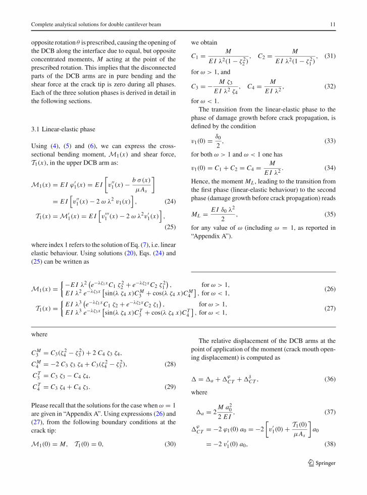
For the interface we use a bi-linear CZM consist-ing of a linear-elastic branch and a linear softeningbranch, followed by zero tractions for relative displace-ments greater than the critical value δc, as shown onthe right-hand side in Fig. 2. Here we emphasise thatCCM solutions presented in this paper are not generalsolutions valid for any shape of the traction–separationlaw of the CZM, but are only valid when the interfacebehaviour can be assumed as bi-linear with progressivedamage. Thus, for a bi-linear CZM law the solutionwill be obtained for three different phases in the crackpropagation process, which is explained in detail in thefollowing subsection.

123

Complete analytical solutions for double cantilever beam 7

Fig. 1 DCB with aprescribed rotations and bprescribed displacement

2.1 Three-phase solution

In order to solve the problemof aDCBwith an interfacewith embedded bi-linear CZM, the usual approach isto develop solutions for three different phases (Stigh1988; de Morais 2013; Dimitri et al. 2017) which arenamely: (i) linear-elastic behaviour, (ii) damage growthbefore crack propagation and (iii) crack propagation.The solution for each of these phases is derived in detailin the following sections according to Fig. 2, whereonly the upper half of the beam is shown. The origin ofthe co-ordinate system is in the left-most undamagedpoint for every phase, and it is moving to the right-hand side as the damage at the interface increases andthe crack propagates. Transversal displacements of theupper arm are denoted by v1(x) for x > 0 and by v2(x)otherwise for reasons which will be explained in Sect.2.2.

2.1.1 Linear-elastic behaviour

In this phase the entire DCB acts as a linear-elasticbody, which means that besides the DCB arms (with alinear-elastic constitutive law), the interface behaviouris linear-elastic, too. For all points at the interfaceundergoing separation (including points A and B inFig. 2a), δ(x) < δ0 and σ(x) < σmax , where δ0 andσmax are linear-elastic limit values of the separation δ

and the traction σ on the interface, respectively. Thisalsomeans that, as long as δ(x) < δ0 andσ(x) < σmax ,no energy dissipation (damage) at the interface occursand the initial (undeformed and undamaged) configu-ration can be recovered if the load is removed. Once at

the crack tip δ(0) = δ0, we enter a new phase wheredamage at the interface starts to develop. This phase isexplained in the following section.

It is well known that a zone of compressive stresses(σ(x) < 0, resulting in δ(x) < 0) ahead of the crack tipexists in a DCB (Alfano and Crisfield 2001; de Morais2015; Dimitri et al. 2017). However, our CZM assumesthat in compression no softening (or damage) occurs,and the behaviour is still linear elastic. In Fig. 2a wecan see that point C experiences negative (compres-sive) contact tractions and negative relative displace-ments at the interface. For a zero-thickness adhesivelayer this results in a non-physical overlapping of thearms, which in our model is allowed and does not cre-ate any additional stresses. But because the interfacethickness in our model does not influence the results(although it is well know that in reality a different thick-ness of the same adhesive results in a different struc-tural behaviour) and we can assume that the interface issufficiently thick to prevent the arms coming in directcontact.

2.1.2 Damage growth before crack propagation

In this phase, the interface can be divided in two zones.In the first zone, just ahead of the crack tip, damageis developing (although the crack is still not propagat-ing) and δ(x) ∈ [δ0, δc), where x ∈ (−Lcz, 0]. In thesecond zone interface behaviour is again linear-elastic,i.e. δ(x) < δ0, where x > 0. Note that according toFig. 2b, x = −Lcz corresponds to the initial crack tipand x = 0 corresponds to the point where the first andthe second zone meet. In this phase, the damage builds

123

8 L. Škec et al.

Fig. 2 Three phases of the problem solution with the deformedshape of the interface (shaded in grey) given on the left-handside, and the position of characteristic points (A, B and C) in the

σ − δ diagram given on the right-hand side. Point A representsthe initial crack tip (a = a0) in a and b, and the crack tip at anyposition where a > a0 in c

up with loading and Lcz increases from 0 (correspond-ing to δ(−Lcz) = δ(0) = δ0) to a certain limit value(corresponding to δ(−Lcz) = δc) at which the crackbegins to propagate. Note that, according to Fig. 2b,the σ −δ relationship in the first zone is also linear, butwith softening (damage).

2.1.3 Crack propagation

This phase is similar to the previous phase (Sect. 2.1.2)with the difference that here the relative displace-ment at the current crack tip, δ(−Lcz) = δc, remainsunchanged during the whole phase. For a DCB withprescribed rotations the cohesive zone length remainsconstant for any position of the crack (steady-statecrack propagation), while for a DCB with prescribed

displacement the cohesive zone length will change(non-steady-state crack propagation). Thus, when thecrack propagation is steady state the deformed shapeof the interface shown in Fig. 2c, and the contact trac-tion distribution over the interface, σ(x), simply trans-late to the right-hand side. This is why point A in Fig.2c is the point at the interface where the crack tip iscurrently located. When the crack propagation is notsteady-state, we still have δ(−Lcz) = δc and δ(0) = δ0for any position of the crack tip, but the deformedshape and the contact traction distribution at the inter-face (including Lcz) change as the crack propagates.The part of the interface which has been completelydamaged (σ(x) = 0) is excluded from the domain ofthe solution for v2(x) and becomes a part of the DCBarm.

123

Complete analytical solutions for double cantilever beam 9

2.2 Solutions of differential equations of the problem

The differential equation of the Timoshenko beamreads

vIV(x) − 1

E Iq(x) + 1

μAsq ′′(x) = 0, (2)

where E I is the bending stiffness (with secondmomentof area I = b h3/12), μAs is the shear stiffness (withcorrected shear area As = b h ks , where ks is the shearcorrection coefficient) and q(x) is distributed trans-verse load along the beam axis, assumed to be positivewhen pointing upwards. Furthermore, in accordancewith the co-ordinate system from Fig. 1, we have

q(x) = T ′(x), (3)

ϕ(x) = v′(x) + γ (x) = v′(x) + T (x)

μAs, (4)

where T (x), γ (x) and ϕ(x) are the shear force, shearstrains and cross-sectional rotation, respectively. Weassume that the self-weight of the DCB arms is negli-gible compared to the magnitude of the external forcesor moments acting on the DCB. Therefore, only con-tact tractions will act on the arms as a distributed load,and thus

q(x) = −b σ(x), (5)

where the negative sign appears because positive (ten-sile) contact tractions at the upper arm are pointeddownwards. The part of the DCB arms separated by theinitial crack, orwhere the interface has been completelydamaged, is excluded from the domain of the solutionv(x). However, the moment or the force applied at thepoint of the prescribed rotationor displacement, respec-tively, (which is outside of the mentioned domain) aretaken into account via the boundary conditions at thecrack tip. This will be explained in detail in the follow-ing sections.

We define σ(x) according to the traction–separationlaw of the CZM. Thus, in our case we will define σ(x)separately for the linear-elastic (δ(x) ≤ δ0) and for thelinear softening part (δ0 < δ(x) ≤ δc) as

σ(x) =

⎧⎪⎨

⎪⎩

σmaxδ(x)

δ0, if δ(x) ≤ δ0,

σmaxδc − δ(x)

δc − δ0, if δ0 < δ(x) ≤ δc.

(6)

Substituting (6) in (5) and then in (2) and taking intoaccount (1) we obtain two differential equations

vIV(x) − 2 ω λ2 v′′(x)

+ λ4 v(x) = 0, if v(x) ≤ δ0

2, (7)

vIV(x) + 2 ψκ2 v′′(x) − κ4v(x)

+ κ4 δc

2= 0, if

δ0

2< v(x) ≤ δc

2, (8)

where

λ = 4

√2 b σmax

E I δ0, ω = E I

μAs

λ2

2, (9)

κ = 4

√2 b σmax

E I (δc − δ0), ψ = E I

μAs

κ2

2. (10)

Equation (7) is used in all phases on the undamagedpart of the interface (x ≥ 0), while Eq. (8) is used onlyin phases 2 and 3 on the damaged part of the interface(x ∈ [−Lcz, 0)). We will denote the solutions of Eqs.(7) and (8) by v1(x) and v2(x), respectively, and derivethem in the following sections.

2.2.1 Solution on the undamaged part of the interface

Assuming the solution of Eq. (7) in a form v1(x) =er x , where r is a constant, results in a characteristicequation with four roots, namely

r1 = λ ζ1, r2 = −λ ζ1, r3 = λ ζ2, r4 = −λ ζ2,

(11)

where

ζ1 =√

ω +√

ω2 − 1, ζ2 =√

ω −√

ω2 − 1. (12)

Since ω ≥ 0, we will have all real roots for ω > 1,all complex roots for ω < 1 and multiple real roots forω = 1. For each of these cases, we can now give:

1. The solution of Eq. (7) for ω > 1:

v1(x) = e−λζ1xC1 + e−λζ2xC2 + eλζ1xC1

+ eλζ2xC2, x ≥ 0, (13)

where C1,C2,C1 andC2 are integration constants.

123

10 L. Škec et al.

2. The solution of Eq. (7) for ω < 1:

v1(x) = e−λζ3x [sin(λ ζ4 x)C3 + cos(λ ζ4 x)C4]

+ eλζ3x[sin(λ ζ4 x)C3 + cos(λ ζ4 x)C4

], x ≥ 0,

(14)

where

ζ3 =√1 + ω

2, ζ4 =

√1 − ω

2, (15)

and C3, C4, C3 and C4 are integration constants.Note that because of

ζ1 ζ2 = 1, and (ζ1 + ζ2)2 = 2(ω + 1), (16)

we have

ζ3 = ζ1 + ζ2

2, ζ4 = i

ζ2 − ζ1

2. (17)

3. The solution of Eq. (7) for ω = 1:

v1(x) = e−λx (C5 + C6 x) + eλx (C5

+C6 x), x ≥ 0, (18)

where C5,C6,C5 and C6 are integration constants.

In our approach we will assume that during crackpropagation the crack tip is always sufficiently distantfrom the right-hand end of the DCB, in a way thatany boundary conditions at the right-hand end (freeor clamped) do not influence the results. This is equiv-alent to assuming a semi-infinite DCB. Therefore thedomain of the undamaged part of the interfacewill haveboundary conditions at x = 0 and x = ∞, where wecan write:

v1(∞) = 0, ϕ1(∞) = 0, (19)

where ϕ1(x) is the cross-sectional rotation on theundamaged part of the interface. According to Tim-oshenko beam theory ϕ1(x) = v′

1(x) + T1(x)/μAs ,where T1(x) is the cross-sectional shear force on theundamaged part of the interface. Because T1(∞) = 0,applying boundary conditions (19) to solutions (13),(14) and (18) gives Ci = 0, where i = 1, . . . , 6. Thus,the solution of Eq. (7) for a semi-infinite DCB can bewritten in a general form as

v1(x) =⎧⎨

⎩

e−λζ1xC1 + e−λζ2xC2, for ω > 1,e−λζ3x [sin(λ ζ4 x)C3 + cos(λ ζ4 x)C4] , for ω < 1,e−λx (C5 + x C6), for ω = 1,

(20)

where x ≥ 0.

Remark 2.1 For the sake of simplicity and because ofthe extreme unlikelihood that the value ω = 1 occursin a real case, the solutions in the following sectionsare given only for the cases when ω > 1 and ω < 1.However, the results for ω = 1 are given separatelyin “Appendix A” for completeness. In the numericalexamples presented in Sect. 7 we will show that, unlikestated in de Morais (2015), all solutions from Eq. (20)are possible for realistic values of geometrical andmaterial properties of a DCB.

2.2.2 Solution on the damaged part of the interface

Assuming the solution of Eq. (8) in a form v2(x) = etx ,where t is a constant, results in a characteristic equationwith four roots, namely

t1 = κ ξ1, t2 = −κ ξ1, t3 = i κ ξ2, t4 = −i κ ξ2, (21)

where

ξ1 =√

−ψ +√

ψ2 + 1, ξ2 =√

ψ +√

ψ2 + 1.

(22)

Since ξ1 and ξ2 are real for any value of ψ , roots t1and t2 are always real, whereas t3 and t4 are alwaysimaginary. Thus, the solution of Eq. (8) can be writtenas

v2(x) = sin(κ ξ2 x)D1 + cos(κ ξ2 x)D2

+ sinh(κ ξ1 x)D3 + cosh(κ ξ1 x)D4 + δc

2,

(23)

for x ∈ [−Lcz, 0], where Di , i = 1, . . . , 4 are integra-tion constants.

In the following sections, the problem is solved andthe integration constants are determined for each phasefor aDCBwith either prescribed rotations or prescribeddisplacement.

3 DCB with prescribed rotations

Consider a DCBwith prescribed rotations as illustratedin Fig. 1a. At the left-hand end of each arm an equal, but

123

Complete analytical solutions for double cantilever beam 11

opposite rotation θ is prescribed, causing the opening ofthe DCB along the interface due to equal, but oppositeconcentrated moments, M acting at the point of theprescribed rotation. This implies that the disconnectedparts of the DCB arms are in pure bending and theshear force at the crack tip is zero during all phases.Each of the three solution phases is derived in detail inthe following sections.

3.1 Linear-elastic phase

Using (4), (5) and (6), we can express the cross-sectional bending moment, M1(x) and shear force,T1(x), in the upper DCB arm as:

M1(x) = E I ϕ′1(x) = E I

[

v′′1 (x) − b σ(x)

μAs

]

= E I[v′′1 (x) − 2 ω λ2 v1(x)

], (24)

T1(x) = M′1(x) = E I

[v′′′1 (x) − 2 ω λ2v′

1(x)],

(25)

where index 1 refers to the solution of Eq. (7), i.e. linearelastic behaviour. Using solutions (20), Eqs. (24) and(25) can be written as

M1(x) ={−E I λ2

(e−λζ1xC1 ζ 2

2 + e−λζ2xC2 ζ 21

), for ω > 1,

E I λ2 e−λζ3x[sin(λ ζ4 x)CM

3 + cos(λ ζ4 x)CM4

], for ω < 1,

(26)

T1(x) ={E I λ3

(e−λζ1xC1 ζ2 + e−λζ2xC2 ζ1

), for ω > 1,

E I λ3 e−λζ3x[sin(λ ζ4 x)CT

3 + cos(λ ζ4 x)CT4

], for ω < 1,

(27)

where

CM3 = C3(ζ

24 − ζ 2

3 ) + 2 C4 ζ3 ζ4,

CM4 = −2 C3 ζ3 ζ4 + C3(ζ

24 − ζ 2

3 ), (28)

CT3 = C3 ζ3 − C4 ζ4,

CT4 = C3 ζ4 + C4 ζ3. (29)

Please recall that the solutions for the case whenω = 1are given in “Appendix A”. Using expressions (26) and(27), from the following boundary conditions at thecrack tip:

M1(0) = M, T1(0) = 0, (30)

we obtain

C1 = M

E I λ2(1 − ζ 22 )

, C2 = M

E I λ2(1 − ζ 21 )

, (31)

for ω > 1, and

C3 = − M ζ3

E I λ2 ζ4, C4 = M

E I λ2, (32)

for ω < 1.The transition from the linear-elastic phase to the

phase of damage growth before crack propagation, isdefined by the condition

v1(0) = δ0

2, (33)

for both ω > 1 and ω < 1 one has

v1(0) = C1 + C2 = C4 = M

E I λ2. (34)

Hence, the moment ML , leading to the transition fromthe first phase (linear-elastic behaviour) to the secondphase (damage growth before crack propagation) reads

ML = E I δ0 λ2

2, (35)

for any value of ω (including ω = 1, as reported in“Appendix A”).

The relative displacement of the DCB arms at thepoint of application of the moment (crack mouth open-ing displacement) is computed as

� = �a + �ϕCT + �δ

CT , (36)

where

�a = 2M a202 E I

, (37)

�ϕCT = −2 ϕ1(0) a0 = −2

[

v′1(0) + T1(0)

μAs

]

a0

= −2 v′1(0) a0, (38)

123

12 L. Škec et al.

�δCT = 2 v1(0), (39)

are the crack mouth opening displacements due tobending of the arms behind the crack tip, rotation ofthe crack tip and opening at the crack tip, respectively.Note that displacement � is the total opening of thecrackmouth, and it takes into account both arms, whichis why factor 2 is used in expressions (37)–(39). Equa-tion (36) can be now rewritten as

�(M) = 2

[M a202 E I

− v′1(0)a0 + v1(0)

]

, M ≤ ML ,

(40)

where v1(0) is defined in (34) and v′1(0) can be obtained

from (20) as

v′1(0) = −λ(ζ1 C1 + ζ2 C2) = λ(ζ4 C3 − ζ3 C4)

= −M√2(1 + ω)

E I λ, (41)

in which the final expression is valid for any value ofω. It follows that

�(M)

= M a20E I

[

1 + 2√2(1 + ω)

a0 λ+ 2

a20λ2

]

, M ≤ ML ,

(42)

is obviously linear for any value ofω (includingω = 1,as reported in “Appendix A”).

We will use Eq. (36) as a general solution for thecrack mouth opening displacement of a DCB, whichis valid for all three solutions phases, not only for aDCB with prescribed rotations. However, in general�a ,�

ϕCT and�δ

CT are computed differently each time.The final forms of functions v1(x), v′

1(x), ϕ1(x),M1(x), T1(x) and σ(x) for this phase are given in“Appendix E.1”.

3.2 Phase of damage growth before crack propagation

In this phase, a cohesive (or damage-process) zone isdeveloping in front of the crack tip. As already men-tioned, for the cohesive zone (x ∈ [−Lcz, 0]) we usethe solution (23), whereas for the zone of linear-elasticbehaviour (x ≥ 0) we use the solution (20).

There are six constants to determine, two for theundamaged part (C1 and C2 if ω > 1, or C3 and C4 if

ω < 1) and four for the damaged part (D1, . . . , D4) inorder to obtain the complete solution. First, from

v1(0) = δ0

2, (43)

we obtain

C1 + C2 = C4 = δ0

2. (44)

We then impose the continuity conditions at the originof the co-ordinate system:

v1(0) = v2(0), ϕ1(0) = ϕ2(0), M1(0) = M2(0),

T1(0) = T2(0), (45)

where ϕ2(x) is the cross-sectional rotation on the dam-aged part of the interface,M1(x) and T1(x) are definedaccording to (26) and (27), respectively, and

M2(x) = E I ϕ′2(x)

= E I

[

v′′2 (x) + 2 ψ κ2

(

v2(x) − δc

2

)]

,

(46)

T2(x) = M′2(x) = E I

[v′′′2 (x) + 2 ψ κ2v′

2(x)],

(47)

are the cross-sectional bending moment and the shearforce on the damaged part of the interface, respectively.Using the solution (23) these expressions can bewrittenas

M2(x) = E I κ2 {−ξ21 [sin(κ ξ2 x)D1 + cos(κ ξ2 x)D2]

+ ξ22 [sinh(κ ξ1 x)D3 + cosh(κ ξ1 x)D4]}, (48)

T2(x) = E I κ3 {−ξ1 [cos(κ ξ2 x)D1 − sin(κ ξ2 x)D2]

+ ξ2 [cosh(κ ξ1 x)D3 + sinh(κ ξ1 x)D4]} , (49)

where the property ξ1 ξ2 = 1 is used to simplify theexpressions. Note also that, because ϕ2(x) = v′

2(x) +T2(x)/μAs and T1(0) = T2(0), the condition ϕ1(0) =ϕ2(0) can bewritten as v′

1(0) = v′2(0). From conditions

(45) we can then express constants Di (i = 1, . . . , 4),in terms of C2 for ω > 1 or C3 for ω < 1 in thefollowing general form

Di (Lcz) = Di1 + C j (Lcz) Di2

D0, i = 1, . . . , 4, (50)

where j = 2 for ω > 1 and j = 3 for ω < 1, Di1

and Di2 are constants depending on the value of ω, asexplained below, and

D0 = 2(ξ21 + ξ22 ) ≡ 4(ψ2 + 1). (51)

123

Complete analytical solutions for double cantilever beam 13

As indicated in (50) and explained later, Di and C j arenot true constants, but parameters depending on Lcz . Ifwe set

ζ 1 ={√

ω + √ω2 − 1, if ω > 1

0, otherwise,

ζ 2 ={√

ω − √ω2 − 1, if ω > 1

0, otherwise,

ζ 3 =⎧⎨

⎩

√1 + ω

2, if ω < 1

0, otherwise,

ζ 4 =⎧⎨

⎩

√1 − ω

2, if ω < 1

0, otherwise, (52)

the values of the constants Di1 and Di2 (i = 1, . . . , 4)are the following:

D11 = −δ0 η ξ1

[ζ 1(ξ

22 + η2 ζ

22) + ζ 3(ξ

22 + η2)

],

D12 = 2 η ξ1(ξ22 − η2)(ζ 1 − ζ 2 + ζ 4),

D21 = δ0 η2(ζ22 + ζ

23 − ζ

24 − η2 ξ22 ),

D22 = 2 η2(ζ21 − ζ

22 + 2 ζ 3 ζ 4),

D31 = −δ0 η ξ2

[ζ 1(ξ

21 − η2 ζ

22) + ζ 3(ξ

21 − η2)

],

D32 = 2 η ξ2(ξ21 + η2)(ζ 1 − ζ 2 + ζ 4),

D41 = −δ0 η2(ζ22 + ζ

23 − ζ

24 + η2 ξ21 ),

D42 = −D22, (53)

with η = λ/κ . Parameter C j (Lcz) is determined fromthe last (sixth) remaining boundary condition

T2(−Lcz) = 0, (54)

as

C j (Lcz) = −ξ1[D21 s2(Lcz) + D11 c2(Lcz)

] + ξ2[D41 sh1(Lcz) − D31 ch1(Lcz)

]

ξ1[D22 s2(Lcz) + D12 c2(Lcz)

] + ξ2[D42 sh1(Lcz) − D32 ch1(Lcz)

] , (55)

where j = 2, 3 and

s2(Lcz) = sin(Lcz κ ξ2), c2(Lcz) = cos(Lcz κ ξ2),

sh1(Lcz) = sinh(Lcz κ ξ1), ch1(Lcz) = cosh(Lcz κ ξ1).

(56)

To summarise, parameters Di (Lcz) needed to definedisplacement field (23) within the damaged zone are

determined from (50) for any value of ω, whereC j (Lcz) is computed from (55). For ω > 1, C2(Lcz)

is defined according to (55) ( j = 2) and C1(Lcz) isobtained from (44) as C1(Lcz) = δ0/2−C2(Lcz). Forω < 1, C3(Lcz) is computed from (55) ( j = 3) and,according to (44), C4 = δ0/2 for any value of Lcz .

The value of the applied moment M is increasingduring this phase and Lcz is strictly increasing withincreasing M . Hence, M will also depend on Lcz . Thisfunction, M(Lcz), can be obtained from the followingcondition

M(Lcz) = M2(−Lcz), (57)

with M2(−Lcz) computed from (48). Obviously, Lcz

and M(Lcz) can increase only up to a certain limit afterwhich the crack begins to propagate and we enter thethird phase of the solution. The crack starts to propagateas soon as the relative opening at the crack tip reachesthe critical value δc or

v2(−Lcz) = δc

2. (58)

This condition represents a highly non-linear equa-tion in terms of Lcz , which contains trigonometric andhyperbolic functions, and cannot be solved in a closedform. Thus, a numerical solver is needed and in thepresent work we use a simple Newton-Raphson itera-tive procedure (more information regarding the numer-ical solver is given in Sect. 7). We will denote the solu-tion of (58) as Lcz and the maximum applied momentby Mmax = M(Lcz).

According to (36), where �a can be still definedaccording to (37), but now

�ϕCT = −2 v′

2(−Lcz) a0, (59)

�δCT = 2 v2(−Lcz), (60)

the crack mouth opening can be computed as

�(Lcz) = 2

[M(Lcz) a20

2 E I

− v′2(−Lcz) a0 + v2(−Lcz)

], Lcz ∈ [0, Lcz], (61)

where v2(−Lcz) and v′2(−Lcz) are evaluated from (23)

at the co-ordinate x = −Lcz .

123

14 L. Škec et al.

3.3 Crack propagation phase

In the previous phase (damage growth before crackpropagation) the applied moment is increasing fromML to M(Lcz) = Mmax . Since for a DCB with pre-scribed rotations there is no shear force at the crack tipduring all phases, itmeans that only the appliedmomentM (same at the crack tip as at the point of application) isresponsible for crack propagation. Obviously, the crackwill propagate when the applied moment reaches thevalue Mmax and this value will not change as the crackpropagates. A constant value of Mmax during crackpropagation implies that the boundary conditions at thecrack tip remain constant and that Lcz = Lcz , duringcrack propagation. This kind of behaviour is known as‘steady-state crack propagation’. Thus, unlike in theprevious phase, in this phase Lcz is not a variable.

The interface is again divided in two domains, theundamaged one (x ≥ 0), where function v1(x) isdefined according to (20), and the damaged one (x ∈[−Lcz, 0]), where function v2(x) is defined accordingto (23). Continuity conditions (45) still apply and con-stants Di are now obtained as

Di = Di1 + C j Di2

D0, i = 1, . . . , 4, j = 2, 3, (62)

which is similar, but not equivalent to (50), because Di

andC j are now true constants and not functions of Lcz .On the other hand, constants D0, Di1 and Di2 are stilldefined according to (51) and (53). Constant C j is nowdetermined from the condition

v2(−Lcz) = δc

2(63)

as

C j = D11 s2 − D21 c2 + D31 sh1 − D41 ch1−D12 s2 + D22 c2 − D32 sh1 + D42 ch1

, (64)

where j = 2, 3 and

s2 = s2(Lcz) = sin(Lcz κ ξ2),

c2 = c2(Lcz) = cos(Lcz κ ξ2),

sh1 = sh1(Lcz) = sinh(Lcz κ ξ1),

ch1 = ch1(Lcz) = cosh(Lcz κ ξ1). (65)

To summarise, constants Di (i = 1, . . . , 4) aredetermined from (62) for any value of ω. For ω > 1,C2 = C j , where C j is defined in (64) and C1 =δ0/2 − C2, according to (44). For ω < 1, C3 = C j ,

where C j is defined in (64) and C4 = δ0/2, accordingto (44).

Since in the crack propagation phase the appliedmoment remains constant, it can be computed from(57) as Mmax = M(Lcz). Crack mouth opening can bethen computed as

�(a) = 2

[Mmax a2

2 E I− v′

2(−Lcz)a

+ v2(−Lcz)], a ≥ a0, (66)

where, theoretically, the value of a can go to infinity.Note also that v2(−Lcz) and v′

2(−Lcz) are constantsand thus the function �(a) in this phase is quadratic.Because in this phase M does not change, � does notdepend on M and we cannot define �(M).

4 DCB with prescribed displacement

In this section we consider a DCB with prescribed dis-placement where, according to Fig. 1b, at the left-handend the bottom arm is pinned, whereas the upper arm ispulled upwards. In order to prescribe a displacement�at the left-hand side of the upper arm, a vertical forceF must be applied at the same place and in the samedirection. Thus, unlike in the case of a DCB with pre-scribed rotations, at the cracked portion of a DCB withprescribed displacement there is bending and shear inthe arms, which will make the problem slightly morecomplex. Furthermore, because the crack propagationin the case of a DCB with prescribed displacement isnot steady-state (Lcz changes during crack propaga-tion), the solution for the third phase (crack propaga-tion) will be also more complex, compared to the caseof DCBwith a prescribed rotations where Lcz = Lcz isconstant during crack propagation. Each phase of thesolution is explained in detail in following sections.

4.1 Linear-elastic phase

In this phase the boundary conditions at the crack tipread

M1(0) = F a0, T1(0) = F, (67)

from which, using (26) and (27), constants

C1 = F(ζ1 + a0 λ)

E I λ3(1 − ζ 22 )

, C2 = F(ζ2 + a0 λ)

E I λ3(1 − ζ 21 )

, (68)

123

Complete analytical solutions for double cantilever beam 15

for ω > 1 and

C3 = − F(ζ 23 − ζ 2

4 + a0 λ ζ3)

E I λ3 ζ4,

C4 = F(a0 λ + 2 ζ3)

E I λ3, (69)

for ω < 1 are determined. The limit value of the force,FL , at which damage starts to develop at the interfaceis obtained from condition (33), which gives

v1(0) = F

E I λ3

(a0 λ + √

2(ω + 1))

= δ0

2, (70)

so that

FL = E I δ0 λ3

2(a0 λ + √

2(1 + ω)) . (71)

Note that a real value of FL is obtained for any valueof ω (including ω = 1, as reported in “Appendix A”).The same applies to v1(0) in (70).

The prescribed displacement is in this case equal tothe crackmouth opening�, whichwe define accordingto (36), where now we have

�a = 2

(F a303 E I

+ F a0μAs

)

, (72)

�ϕCT = −2 ϕ1(0) a0 = −2 a0

[

v′1(0) + F

μAs

]

, (73)

�δCT = 2 v1(0). (74)

The crack mouth opening displacement can be thenwritten as

�(F) = 2

[F a303 E I

− v′1(0) a0 + v1(0)

]

, F ≤ FL ,

(75)

where v1(0) is defined in (70) and

v′1(0) = − F

E I λ2

(2 ω + 1 + a0 λ

√2(1 + ω)

). (76)

Note that although the terms responsible for sheardeformations in (72) and (73) cancel out in (75), sheardeformability is taken into account through ω in (70)and (76). Equation (76) is valid for any value of ω

(including ω = 1, as reported in “Appendix A”). Equa-tion (75) can be finally written as

�(F) = 2 F a303 E I

{

1 + 3√2(1 + ω)

(a0λ)3

[√2(1 + ω)a0 λ

+ (a0 λ)2 + 1]}

, F ≤ FL . (77)

The final forms of functions v1(x), v′1(x), ϕ1(x),

M1(x), T1(x) and σ(x) for this phase are given in“Appendix E.2”.

4.2 Phase of damage growth before crack propagation

In this phase, we divide the interface into the undam-aged domain (x ≥ 0) and the damaged domain (x ∈[−Lcz, 0]), and continuity conditions (45) between thetwo still apply. Using these conditions and condition(43) we can again define parameters Di (Lcz), wherei = 1, . . . , 4, using (50) and constantsC1 andC4 using(44). However, solution (55) for parameters C j (Lcz),where j = 2, 3, is no longer valid because the boundarycondition (54) in the case of prescribed displacementbecomes

T2(−Lcz) = F(Lcz), (78)

which cannot give us the solution for C j (Lcz) becausethe function F(Lcz) is yet unknown. An additionalboundary condition

M2(−Lcz) = F(Lcz) a0, (79)

gives

F(Lcz) = M(Lcz)

a0, (80)

whereM(Lcz) is defined in (57). Now, using (80), from(78) it follows that

C j (Lcz)

= β1 s2(Lcz) + β2 c2(Lcz) + β3 sh1(Lcz) + β4 ch1(Lcz)

β5 s2(Lcz) + β6 c2(Lcz) + β7 sh1(Lcz) + β8 ch1(Lcz),

(81)

where j = 2, 3 and

β1 = ξ21 (D11 + a0 κ ξ2 D21)

β2 = ξ21 (−D21 + a0 κ ξ2 D11),

β3 = ξ22 (−D31 + a0 κ ξ1 D41)

β4 = ξ22 (D41 − a0 κ ξ1 D31),

β5 = −ξ21 (D12 + a0 κ ξ2 D22)

β6 = ξ21 (D22 − a0 κ ξ2 D12),

β7 = ξ22 (D32 − a0 κ ξ1 D42)

β8 = ξ22 (−D42 + a0 κ ξ1 D32). (82)

Let us recall that, because of definitions (52) and(53), solution (81) for C j (Lcz) automatically returnsthe value of C2(Lcz) for ω > 1 and C3(Lcz) forω < 1. Thus, in the case when ω > 1 we computeC2(Lcz) from (81) and then C1(Lcz) follows from (44)as C1(Lcz) = δ0/2−C2(Lcz). For ω < 1 we compute

123

16 L. Škec et al.

C3(Lcz) from (81), whereas C4 is defined in (44) asC4 = δ0/2. Using solution (81), from (50) we can thenobtain parameters Di (Lcz), where i = 1, . . . , 4, whichare needed to compute M(Lcz) (see (57)) and finallyF(Lcz) according to (80).

As explained in Sect. 3.2, in this phase Lcz growsfrom0 to a value corresponding to the initiation of crackpropagation, i.e. transition to the third phase. This is amaximum value for Lcz , because during crack propa-gation Lcz decreases and asymptotically tends to amin-

imum value when a → ∞, as is discussed in the nextsection. Therefore, this initial maximum value of Lcz

at the initiation of crack propagation will be denoted byLmaxcz . In order to obtain this value, the same approach

as for a DCB with prescribed rotations is followed, i.e.condition (58) is imposed. This is again a highly non-linear equation in terms of Lcz , which is solved numer-ically (in our approach Newton-Raphson procedure isused).

The prescribed displacement in the second phase canbe computed as

�(Lcz) = 2

[F(Lcz) a303 E I

− v′2(−Lcz) a0

+ v2(−Lcz)

]

, Lcz ∈ [0, Lmaxcz ], (83)

where v2(−Lcz) and v′2(−Lcz) are evaluated using (23)

at the co-ordinate x = −Lcz .

4.3 Crack propagation phase

As previously mentioned, in the case of a DCB withprescribed displacement, the cohesive zone lengthdecreases during crack propagation from Lmax

cz asymp-totically approaching a lower limit value Lmin

cz . Thismeans that the crack propagation is not steady state,but it approaches steady state for infinitely long cracks(Dimitri et al. 2017). Because Lmin

cz corresponds to asteady-state crack propagation, it must have the samevalue as Lcz found in the identical DCB loaded withprescribed rotations,where crack propagation is alwayssteady state, i.e. Lmin

cz = Lcz . Note that both Lmaxcz

and Lmincz are obtained by numerically solving Eq. (58),

where constants Di (i = 1, . . . , 4) in (23) in the formercase are computed using (81) in (50), whereas in thelatter case they are computed using (55) in (50).

Continuity conditions (45) and condition (43) arestill valid in the third phase, which gives us solution(50). From the condition

v2(−Lcz) = δc

2, (84)

we obtain

C j (Lcz) = D11 s2(Lcz) − D21 c2(Lcz) + D31 sh1(Lcz) − D41 ch1(Lcz)

−D12 s2(Lcz) + D22 c2(Lcz) − D32 sh1(Lcz) + D42 ch1(Lcz), (85)

where j = 2, 3. Note that this expression is differentfrom (64) because here Lcz is a variable.

Function F(Lcz) is obtained from conditions (78)and (49). Note that a is also a function of Lcz , i.e.a = a(Lcz), and can be determined from the condition

M2(−Lcz) = F(Lcz) a(Lcz), (86)

which gives

a(Lcz) = M(Lcz)

F(Lcz), (87)

where M(Lcz) and F(Lcz) are defined according (57)and (78), respectively.

Prescribed displacement can be now expressed as afunction of Lcz as

�(Lcz) = 2

[F(Lcz) a(Lcz)

3

3 E I− v′

2(−Lcz) a(Lcz)

+ v2(−Lcz)

]

, Lcz ∈ [Lmincz , Lmax

cz ], (88)

where v2(−Lcz) and v′2(−Lcz) are evaluated using (23)

at the co-ordinate x = −Lcz .

Remark 4.1 Solutions developed in Sects. 3 and 4(based on Timoshenko beam theory) represent generalsolutions from which we can easily derive three otherparticular cases, for DCBs with either rotations or dis-placement prescribed:

1. Solutions for Euler–Bernoulli beam theory. Thesesolutions are obtained by simply letting the shearmodulus μ → ∞ and are presented in “AppendixB”.

2. Solutions for a linear-elastic interface with brittlefailure. These solutions, presented in Sect. 5 for

123

Complete analytical solutions for double cantilever beam 17

Timoshenko beam theory and in “Appendix C” forEuler–Bernoulli beam theory, are obtained by let-ting δc → δ0, which means that there is no damagebefore crack propagation, i.e. only the first and thethird solution phases remain.

3. LEFM solutions. These solutions, given both forTimoshenko beam theory in Sect. 6 and Euler–Bernoulli beam theory in “Appendix C”, are obtai-ned from the solutions for a linear-elasticCZMwithbrittle failure by letting δ0 → 0.

5 Analytical solutions for a DCB withlinear-elastic interface with brittle failure (EBT)

Here we assume that the interface behaves as linear-elastic up to a certain point after which brittle failure(instantaneous loss of cohesion) occurs. In our model,this is achieved by setting δ0 = δc, which removes thesoftening branch in σ −δ diagram shown in Fig. 2. Thisalso means that the second part of the solution (dam-age growth before crack propagation) does not existand that Lcz = 0 during crack propagation.

Referring to Sect. 2.2, we can now rewrite Eq. (6) as

σ(x) =⎧⎨

⎩

σmaxδ(x)

δ0, if δ(x) < δ0,

0, otherwise.(89)

Solutions (20) for v1(x), as well as definitions (9), (12)and (15) for λ, ω and ζi (i = 1, . . . , 4) are still valid.Solution (23) for v2(x) is no longer applicable becauseLcz = 0.

We will now derive the solution for a DCB with abrittle interface, first for a DCB with prescribed rota-tions and then for a DCBwith prescribed displacement.

5.1 DCB with prescribed rotations

The first (linear-elastic) phase of the solution presentedin Sect. 3.1 applies completely to the case of linear-elastic interface with brittle failure. Thus, no modifi-cations in the expressions presented in Sect. 3.1 areneeded.Moreover, this phase can be now called ‘linear-elastic behaviour before crack propagation.’ The crackmouthopeningdisplacement in the phase of crackprop-agation now reads

�(a) = Mmax a2

E I

[

1 + 2√2(1 + ω)

a λ+ 2

a2λ2

]

, a ≥ a0,

(90)

where Mmax is the value of the applied moment whenthe crack starts to propagate corresponding to ML

defined in (35).Since for a linear-elastic interface with brittle failure

the critical energy release rate, Gc, can be written as

Gc = σmax δ0

2, (91)

we can rewrite Eq. (9)1 as

λ = 4

√4 b Gc

E I δ20, (92)

and from (35) obtain

Mmax = √E I b Gc, (93)

which is equivalent to the well-known formula

Gc = M2max

b E I, (94)

used to compute Gc (or the critical value of the J inte-gral, Jc) for a DCB with prescribed rotations (Rice1968; Freiman et al. 1973; Suo et al. 1992; Sørensenet al. 1996). Note that Mmax and Gc are independentof the beam theory used, i.e. the shear deformability ofthe arms does not influence their values.

5.2 DCB with prescribed displacement

For a DCB with prescribed displacement the first partof the solution presented in Sect. 4.1 is entirely valid inthe case when the interface is linear-elastic with brittlefailure. The peak load at the point when the crack startsto propagate, Fmax , corresponds to FL defined in (71),from where by substituting (9) and (92) it follows that

Fmax =√E I b Gc

a0 +√

2λ2

+ E IμAs

. (95)

For the crack propagation phase we have

�(a)=2F(a) a3

3 E I

{

1 + 3√2(1 + ω)

(aλ)3

[√2(1 + ω)a λ

+ (a λ)2 + 1]}

, a ≥ a0, (96)

where

F(a) =√E I b Gc

a +√

2λ2

+ E IμAs

≡ λ√E I b Gc

aλ + √2(1 + ω)

. (97)

123

18 L. Škec et al.

Remark 5.1 Note that presented solutions in terms ofthe applied load and the crack mouth opening displace-ment of a DCB with either prescribed rotations or pre-scribed displacement for the case of a linear-elasticinterface with a brittle failure (EBT) are valid for allvalues of ω (ω < 1, ω = 1 and ω > 1).

6 LEFM solutions for a DCB with prescribedrotations and a DCB with prescribeddisplacement: enhanced simple beam theory(ESBT)

The presented model for a linear-elastic interface witha brittle crack still allows some opening at the interfacein the linear-elastic range before crack starts to propa-gate (δ(x) < δ0). If this initial linear-elastic behaviouris excluded from the model by letting δ0 → 0, whilekeeping Gc constant (which also results in σmax →∞), we obtain solutions equivalent to those given bylinear-elastic fracture mechanics (LEFM). However,we will not a-priori assume that the DCB arms act asif they were clamped at the crack tip, which is usuallydone in the SBTapproach. In thiswaywewill show thatin the limit case of LEFM the arms rotate at the cracktip and in front of it (even though their centre-linesthere remain straight), which means that the clampedconditions at the crack tip cannot be obtained evenfor an infinitely stiff perfectly brittle interface. This isdue exclusively to the shear deformability of the arms,which is accounted for in Timoshenko beam theory. ForEuler–Bernoulli beam theory, the limit case of LEFMindeed corresponds to SBT and the arms do not rotate atthe crack tip and in front of it. Thus, for our LEFM-limitsolution for Timoshenko beam theorywewill adopt theterm ‘enhanced simple beam theory’ (ESBT). In thefollowing subsections we will present only the finalresults for a DCB with prescribed rotations and a DCBwith prescribed displacement, respectively, while thecomplete derivation is given in “Appendix E”.

6.1 DCB with prescribed rotations

As shown in “Appendix E”, in the limit case of LEFMfor any x ≥ 0 we have

vL1 (x) = 0 (98)

v′L1 (x) = M√

E I μAs(H(x) − 1), (99)

ϕL1 (x) = − M√

E I μAse−

√μAsE I x

, (100)

σ L(x) = −M μAs

b E Ie−

√μAsE I x + M

b

√μAs

E ID(x),

(101)

T L1 (x) = −M

√μAs

E I

[

e−√

μAsE I x + (H(x) − 1)

]

,

(102)

M1(x) = Me−√

μAsE I x

, (103)

where D(x) is the Dirac distribution centred at zero(whichmeans that, rigorously speaking, the stress is nota ‘proper’ function but a generalised one), andH(x) isthe Heaviside function defined by:

H(x) ={0 for x ≤ 0,1 for x > 0.

(104)

From the above expressionswecan see that, althoughthere are no relative displacements at the crack tip andin front of it (v1(x) = 0 for any x ≥ 0), rotationsat the crack tip and in front of it are still allowed tooccur when Timoshenko beam theory is used. On theone hand, this result is expected, because it is intu-itive that the independence of rotation and deflection inTimoshenko beam theory allows this theory to capturethe deformation in front of the crack tip, which occursalso in the LEFM limit. This is in contrast with Euler–Bernoulli theory (see “Appendix E.3”), for which theabsence of displacements also means a zero rotationand, ultimately, no deformation in front of the crack tip,but also with the widely used assumption, made in theSBT, that the arms of aDCBact as if theywere clampedat the crack tip. In otherwords, to the best of the authors’knowledge, the ability of Timoshenko’s beam theory tocapture the crack tip rotation also in the LEFM limit hasnot been explored so far, although something similarwas done in EBT for a linear elastic interfacewith finitestiffness and brittle failure (Kanninen 1973; Williams1989). This is why we call our approach ESBT.

Moreover, because the DCB arms deform (rotate) infront of crack tip, contact tractions at the interface, aswell as the shear forces and bending moments in thearms, appear in front of the crack tip, with an expo-nential decay as x → ∞. We can notice that at thecrack tip there is a jump in the shear force (from 0 to

123

Complete analytical solutions for double cantilever beam 19

−M√

μAs/E I ) which corresponds to a transition inthe bending moment diagram from the constant valueM in the cracked portion of the arms to the function(103) in front of the crack tip. This implies that in thelimit case of LEFM there is a concentrated transversalcohesive force exchanged at the crack tip, so that theinterface stress is the sum of a compressive smooth partand the Dirac distribution centred at zero. Because atthe crack tip the cross-sectional rotations of the armsmust be continuous and there is a jump in the shearforce in the arms, the function v′

1(x) is also discontin-uous due to ϕ1(x) = v′

1(x) + T1(x)/μAs .Expressions (98)–(103) are valid only for the phase

of linear-elastic behaviour before crack propagation.However, analogous expressions for the phase of crackpropagation can be obtained simply by substituting Mwith Mmax . Finally, according to (40), we can expressthe crack mouth opening displacement as

�(M) = M a20E I

(

1 + 2

a0

√E I

μAs

)

,

before crack propagation (M ≤ Mmax ),

(105)

�(a) = Mmax a2

E I

(

1 + 2

a

√E I

μAs

)

,

during crack propagation (a ≥ a0), (106)

where Mmax is defined in (93) and the second termin the parentheses in both expressions represents therotation of the arms at the crack tip.

6.2 DCB with prescribed displacement

As shown in “Appendix E”, in the limit case of LEFMfor any x ≥ 0 we have

vL1 (x) = 0, (107)

v′L1 (x) =

(F

μAs+ F a0√

E I μAs

)

(H(x) − 1) (108)

ϕL1 (x) = − F a0√

E I μAse−

√μAsE I x

, (109)

σ L(x) = − F a0 μAs

b E Ie−

√μAsE I x

+ F

b

(

1 + a0

√μAs

E I

)

D(x), (110)

T L1 (x) = −F a0

√μAs

E I

[

e−√

μAsE I x + (H(x) − 1)

]

− F(H(x) − 1), (111)

ML1 (x) = F a0 e

−√

μAsE I x

, (112)

where again we see that even in the limit case of LEFMthe arms rotate at and in front of the crack tipwhenTim-oshenko beam theory is used. The discussion regardingEqs. (98)–(103) also applies here, with the only differ-ence that for aDCBwith prescribed displacement in thecracked portion of the arms we have a constant shearforce and a linear distribution of bending moments.

Note that expressions (107)–(112) are valid only forthe phase of linear-elastic behaviour before crack prop-agation. However, analogous expressions for the crackpropagation phase can be obtained by substituting Fwith F(a) (defined in (116)) and a0 with a.

The crackmouth opening displacement before crackpropagation follows from (75) as

�(F) = 2 F a303 E I

(

1 + 3

a20

E I

μAs

+ 3

a0

√E I

μAs

)

, F ≤ Fmax , (113)

where from (95) we have

Fmax =√E I b Gc

a0 +√

E IμAs

. (114)

During crack propagation the crackmouth opening dis-placement is given by

�(a) = 2 F(a) a3

3 E I

(

1 + 3

a2E I

μAs

+ 3

a

√E I

μAs

)

, a ≥ a0, (115)

where from (97) we have

F(a) =√E I b Gc

a +√

E IμAs

. (116)

Note that in (113) and (115) the term outside the paren-theses represents the arm deflection due to bendingaccording to Euler–Bernoulli beam theory, the secondterm in the parentheses is due to shear deformabilityof the arm, while the third term in the parentheses rep-resents the influence of the rotation of the arms at the

123

20 L. Škec et al.

crack tip. From (116) we can obtain the critical energyrelease rate of a Timoshenko DCBwith prescribed dis-placement as

Gc = F2

b

(a2

E I+ 1

μAs+ 2 a√

E I μAs

)

, (117)

where, for the sake of simplicity, we denote F(a) sim-ply by F . Usually in the SBT solution (Ripling et al.1971; ASTM D3433-99 2012; BS ISO 25217:20092009), only the first two terms in expression (117) aretaken into account because it is assumed that the DCBarms are clamped at the crack tip. The third therm in(117), which takes into account the rotation at the cracktip, to the best of authors’ knowledge, has not beenrecognised so far for the limit case of LEFM. Equation(117) represents the ESBT expression for Gc.

Remark 6.1 In “Appendix E.3” we show that if Euler–Bernoulli beam theory is used, there are no cross-sectional rotations, shear forces or bendingmoments ofthe arms in front of the crack tip. However, singularityof contact tractions at the interface, as well as disconti-nuity of the shear stresses and bending moments in thearms, take place at the crack tip. These conditions areequivalent to clamping DCB arms at the crack tip andexplain why the formulae obtained for the limit case ofLEFM in “Appendix D” indeed correspond to widelyused formulae in SBT.

7 Numerical examples

In this section, for a DCB with a bi-linear CZM atthe interface, the analytical solutions derived in thispaper usingTimoshenko beam theorywill be comparedto the numerical results obtained with an equivalentfinite-element (FE) model, in which the same beamtheory and CZM are used (Škec et al. 2015), and tothe Euler–Bernoulli beam theory analytical solutionsderived in “Appendix B”. The latter will allow us toinvestigate the influence of shear deformability of DCBarms on the results. LEFM solutions obtained in Sect.6 will also be presented as limit cases for a brittle inter-face.

Referring to Fig. 1, we consider a DCB with dimen-sions h = 6 mm, b = 25 mm and a0 = 30 mm.In the present analytical solution, the length of thespecimen is assumed to be infinite (L = ∞), i.e. thecrack is always sufficiently distant from the right-hand(non-loaded) end of the DCB. Material data for the

DCB arms and the interface used in numerical exam-ples is presented in Table 1, where it can be noted thatthe maximum contact traction σmax is varied between7.5 and 120 MPa, while keeping the area under thetraction–separation law, �, constant. This gives us 5cases of different brittleness of the interface, whereσmax = 7.5 MPa represents an extremely ductile caseand σmax = 120 MPa an extremely brittle case. Ratioα = δ0/δc is kept constant in the first set of examples(α = 0.01 for all cases), whereas in the last exampleis varied. Values of E and ν for the DCB arms pre-sented in Table 1 correspond to aluminum, the shearmodulus μ is calculated as for an isotropic material,i.e. μ = 0.5E/(1 + ν), and for the rectangular cross-section considered, ks = 5/6.

The numerical model used is the multi-layer beammodel presented in Škec et al. (2015) where we assumea total length of the specimen L = 200 mm. A totalnumber of 2000 2-node Timoshenko beam elementsare distributed evenly over the upper half of the DCB,meaning that the element length is 0.1 mm. Such afine mesh is used to eliminate or at least minimise theinfluence of discretisation-caused spurious oscillationson the results (Alfano and Crisfield 2001; Škec et al.2015). A 4-node interface element is attached to everybeam FE from x = a0 to x = L making a total of 1700interface elements. The solution is obtained using dis-placement control and Newton-Raphson iterative pro-cedure. Because our numerical model has 4002 degreesof freedom (one transverse displacement and one cross-sectional rotation per node), in each iteration of eachincrement, 4002 linear equations are solved in orderto obtain the cross-head displacement. In our analyt-ical solution, we obtain the cross-head displacementfrom a single closed-form solution. The same appliesto any other quantity we want to obtain. Furthermore,all analytical solutions, unlike the numerical ones, areperfectly smooth.

It is worth noting that the values reported inTable 1 according to (9)2 for σmax = {7.5, 15, 30, 60,120} MPa give ω = {0.32, 0.64, 1.28, 2.57, 5.13}.Thus, we can deduce that in real-life applications bothω < 1 and ω > 1 are possible and therefore the ana-lytical solution should account for both cases.

In the following sections we will present the resultsfor the DCB first with prescribed rotations and thenwith prescribed displacement.

123

Complete analytical solutions for double cantilever beam 21

Table 1 Material data used in the numerical examples. Except in the last example, α = 0.01

E (GPa) ν (–) ks (–) � (N/mm) σmax (MPa) δc (mm) δ0 (mm)

70 1/3 5/6 1 {7.5, 15, 30, 60, 120} 2 �/σmax α δc

Fig. 3 Crack mouth opening displacement–applied moment(�−M) graph for a DCB with prescribed rotations: a rangeof interest, b zoom. A comparison between Timoshenko and

Euler–Bernoulli beam theory for different values of σmax , whereσmax = ∞ represents the LEFM solution

7.1 DCB with prescribed rotations

In Fig. 3, the reactionmoment,M , is plotted against thecrack mouth opening displacement, �. From Fig. 3b,which is the zoom of Fig. 3a, we can first observe thatthe results for Timoshenko beam theory from the ana-lytical and the FE model perfectly match, as expected.We can also note that the results approach the LEFMsolution, which is obtained from our model by lettingδ0 → 0 and σmax → ∞ (as shown in Sect. 5.1), asσmax increases. The same behaviour can be observedwhenEuler–Bernoulli beam theory is used.Differencesbetween Timoshenko and Euler–Bernoulli beam theo-ries are more pronounced for higher values of σmax andespecially for the LEFM solution.

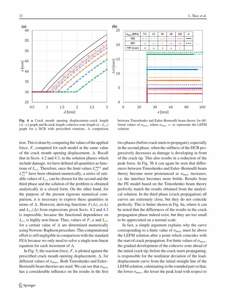
From Fig. 4a it can be clearly seen that the crackwill start to propagate sooner (i.e. for smaller crackmouth opening displacements) when the interface ismore brittle. The numerical model again agrees per-fectly with the analytical solution, and there are somedifferences between Euler–Bernoulli and Timoshenko

beam theory, which again become more significant asσmax increases.

In Fig. 4b we can finally compare the cohesivezone lengths, Lcz , for Timoshenko andEuler–Bernoullibeam theories. As expected, Lcz , which is highly influ-enced by the value of σmax , remains constant duringcrack propagation. Differences between Timoshenkoand Euler–Bernoulli beam theory solutions are noweven more pronounced, especially for more brittlecases. Again, the numerical results match perfectlywith those obtained from the analytical solution forTimoshenko beam theory.

7.2 DCB with prescribed displacement

In this section, the same geometrical and material dataas in Sect. 7.1 is used for the case of a DCB with pre-scribed displacement. We present a comparison of thesolution fromSect. 4 for Timoshenko beam theorywiththe analogous solution for Euler–Bernoulli beam the-ory (presented in “Appendix B.2”) and the LEFM solu-

123

22 L. Škec et al.

Fig. 4 a Crack mouth opening displacement–crack length(�−a) graph and b crack length–cohesive zone length (a−Lcz)graph for a DCB with prescribed rotations. A comparison

between Timoshenko and Euler–Bernoulli beam theory for dif-ferent values of σmax , where σmax = ∞ represents the LEFMsolution

tion.This is donebycomparing thevalues of the appliedforce, F , computed for each model at the same valueof the crack mouth opening displacement, �. Recallthat in Sects. 4.2 and 4.3, in the solution phases whichinclude damage, we have defined all quantities as func-tions of Lcz . Therefore, once the limit values Lmax

cz andLmincz have been obtained numerically, a series of suit-

able values of Lcz can be chosen for the second and thethird phase and the solution of the problem is obtainedanalytically in a closed form. On the other hand, forthe purpose of the present rigorous numerical com-parison, it is necessary to express these quantities interms of �. However, deriving functions F(�), a(�)

and Lcz(�) from expressions given Sects. 4.2 and 4.3is impossible, because the functional dependence onLcz is highly non-linear. Thus, values of F , a and Lcz

for a certain value of � are determined numericallyusingNewton–Raphsonprocedure.This computationaleffort is still negligible in comparison with the standardFEA because we only need to solve a single non-linearequation for each increment of �.

In Fig. 5, the reaction force, F , is plotted against theprescribed crack mouth opening displacement, �, fordifferent values of σmax . Both Timoshenko and Euler–Bernoulli beam theories are used.We can see that σmax

has a considerable influence on the results in the first

twophases (before crack starts to propagate), especiallyin the second phase, when the stiffness of the DCB pro-gressively decreases as damage is developing in frontof the crack tip. This also results in a reduction of thepeak force. In Fig. 5b it can again be seen that differ-ences between Timoshenko and Euler–Bernoulli beamtheory become more pronounced as σmax increases,i.e. the interface becomes more brittle. Results fromthe FE model based on the Timoshenko beam theoryperfectly match the results obtained from the analyti-cal solution. In the third phase (crack propagation) allcurves are extremely close, but they do not coincideperfectly. This is better shown in Fig. 6a, where it canbe noted that the differences of the results in the crackpropagation phase indeed exist, but they are too smallto be appreciated on a normal scale.

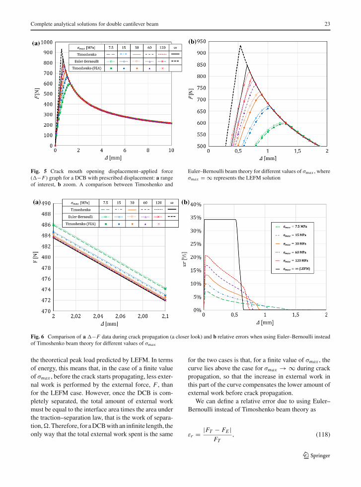
In fact, a simple argument explains why the curvecorresponding to a finite value of σmax must lie abovethe LEFM solution after a point which coincides withthe start of crack propagation. For finite values of σmax ,the gradual development of the cohesive zone ahead ofthe initial crack tip, before the crack starts propagating,is responsible for the nonlinear deviation of the load-displacement curve from the initial straight line of theLEFMsolution, culminating in the rounded part so that,the lower σmax , the lesser the peak load with respect to

123

Complete analytical solutions for double cantilever beam 23

Fig. 5 Crack mouth opening displacement–applied force(�−F) graph for a DCB with prescribed displacement: a rangeof interest, b zoom. A comparison between Timoshenko and

Euler–Bernoulli beam theory for different values of σmax , whereσmax = ∞ represents the LEFM solution

Fig. 6 Comparison of a �−F data during crack propagation (a closer look) and b relative errors when using Euler–Bernoulli insteadof Timoshenko beam theory for different values of σmax

the theoretical peak load predicted by LEFM. In termsof energy, this means that, in the case of a finite valueof σmax , before the crack starts propagating, less exter-nal work is performed by the external force, F , thanfor the LEFM case. However, once the DCB is com-pletely separated, the total amount of external workmust be equal to the interface area times the area underthe traction–separation law, that is the work of separa-tion,�. Therefore, for aDCBwith an infinite length, theonly way that the total external work spent is the same

for the two cases is that, for a finite value of σmax , thecurve lies above the case for σmax → ∞ during crackpropagation, so that the increase in external work inthis part of the curve compensates the lower amount ofexternal work before crack propagation.

We can define a relative error due to using Euler–Bernoulli instead of Timoshenko beam theory as

εr = |FT − FE |FT

, (118)

123

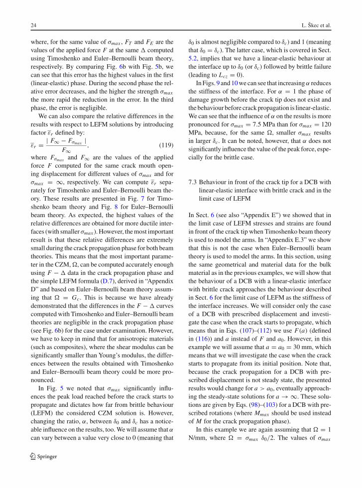
24 L. Škec et al.

where, for the same value of σmax , FT and FE are thevalues of the applied force F at the same � computedusing Timoshenko and Euler–Bernoulli beam theory,respectively. By comparing Fig. 6b with Fig. 5b, wecan see that this error has the highest values in the first(linear-elastic) phase. During the second phase the rel-ative error decreases, and the higher the strength σmax

the more rapid the reduction in the error. In the thirdphase, the error is negligible.

We can also compare the relative differences in theresults with respect to LEFM solutions by introducingfactor εr defined by:

εr = | F∞ − Fσmax |F∞

, (119)

where Fσmax and F∞ are the values of the appliedforce F computed for the same crack mouth open-ing displacement for different values of σmax and forσmax = ∞, respectively. We can compute εr sepa-rately for Timoshenko and Euler–Bernoulli beam the-ory. These results are presented in Fig. 7 for Timo-shenko beam theory and Fig. 8 for Euler–Bernoullibeam theory. As expected, the highest values of therelative differences are obtained for more ductile inter-faces (with smallerσmax ). However, themost importantresult is that these relative differences are extremelysmall during the crack propagation phase for both beamtheories. This means that the most important parame-ter in the CZM,�, can be computed accurately enoughusing F − � data in the crack propagation phase andthe simple LEFM formula (D.7), derived in “AppendixD” and based on Euler–Bernoulli beam theory assum-ing that � = Gc. This is because we have alreadydemonstrated that the differences in the F − � curvescomputed with Timoshenko and Euler–Bernoulli beamtheories are negligible in the crack propagation phase(see Fig. 6b) for the case under examination. However,we have to keep in mind that for anisotropic materials(such as composites), where the shear modulus can besignificantly smaller than Young’s modulus, the differ-ences between the results obtained with Timoshenkoand Euler–Bernoulli beam theory could be more pro-nounced.

In Fig. 5 we noted that σmax significantly influ-ences the peak load reached before the crack starts topropagate and dictates how far from brittle behaviour(LEFM) the considered CZM solution is. However,changing the ratio, α, between δ0 and δc has a notice-able influence on the results, too.Wewill assume that αcan vary between a value very close to 0 (meaning that

δ0 is almost negligible compared to δc) and 1 (meaningthat δ0 = δc). The latter case, which is covered in Sect.5.2, implies that we have a linear-elastic behaviour atthe interface up to δ0 (or δc) followed by brittle failure(leading to Lcz = 0).

In Figs. 9 and 10we can see that increasingα reducesthe stiffness of the interface. For α = 1 the phase ofdamage growth before the crack tip does not exist andthe behaviour before crack propagation is linear-elastic.We can see that the influence of α on the results is morepronounced for σmax = 7.5 MPa than for σmax = 120MPa, because, for the same �, smaller σmax resultsin larger δc. It can be noted, however, that α does notsignificantly influence the value of the peak force, espe-cially for the brittle case.

7.3 Behaviour in front of the crack tip for a DCB withlinear-elastic interface with brittle crack and in thelimit case of LEFM

In Sect. 6 (see also “Appendix E”) we showed that inthe limit case of LEFM stresses and strains are foundin front of the crack tip when Timoshenko beam theoryis used to model the arms. In “Appendix E.3” we showthat this is not the case when Euler–Bernoulli beamtheory is used to model the arms. In this section, usingthe same geometrical and material data for the bulkmaterial as in the previous examples, we will show thatthe behaviour of a DCB with a linear-elastic interfacewith brittle crack approaches the behaviour describedin Sect. 6 for the limit case of LEFM as the stiffness ofthe interface increases. We will consider only the caseof a DCB with prescribed displacement and investi-gate the case when the crack starts to propagate, whichmeans that in Eqs. (107)–(112) we use F(a) (definedin (116)) and a instead of F and a0. However, in thisexample we will assume that a = a0 = 30 mm, whichmeans that we will investigate the case when the crackstarts to propagate from its initial position. Note that,because the crack propagation for a DCB with pre-scribed displacement is not steady state, the presentedresults would change for a > a0, eventually approach-ing the steady-state solutions for a → ∞. These solu-tions are given by Eqs. (98)–(103) for a DCB with pre-scribed rotations (where Mmax should be used insteadof M for the crack propagation phase).

In this example we are again assuming that � = 1N/mm, where � = σmax δ0/2. The values of σmax

123

Complete analytical solutions for double cantilever beam 25

Fig. 7 Timoshenko beam theory. Relative differences between the values of the force F computed for a finite value of σmax and forσmax = ∞ (LEFM solution): a crack initiation, b crack propagation

Fig. 8 Euler–Bernoulli beam theory. Relative differences between the values of the force F computed for a finite value of σmax andfor σmax = ∞ (LEFM solution): a crack initiation, b crack propagation

are varied according to σmax = 10i MPa, where i =0, 1, 2, 3, 4, and the values of δ0 follow from δ0 =2 �/σmax .

In Fig. 11a we see that the cross-sectional rotationsof the upper arm in front of the crack tip, ϕ1(x), reduceas the interface becomes stiffer, but for the limit case ofLEFM, instead of approaching zero, they approach thelimit values given by function (109). According to thisformula, the rotation at the crack tip for the limit caseof LEFM is ϕ(0) = − 0.0025 rad. In Fig. 11b we seehow the contact tractions at the crack tip (σ(0) = σmax )

increase for higher values of σmax and tends to ∞ inthe LEFM limit. In front of the crack tip, there is adistribution of compressive stresses which in the limitcase of LEFM converges to the curve given by Eq.(110) according to which limx→0+ σ(x) = − 105.98MPa.This shows that the area of tensile stresses reducesto zero, while the stress at x = 0 tends to infinity. Itis shown in “Appendix E” that the resultant of thesetensile stresses tends to a finite value. In other words,in the LEFM limit, a Dirac distribution centred at thecrack tip is found.

123

26 L. Škec et al.

Fig. 9 The influence of α = δ0/δc on the � − F results for σmax = 7.5 MPa: a range of interest, b a closer look

Fig. 10 The influence of α = δ0/δc on the � − F results for σmax = 120 MPa: a range of interest, b a closer look

Figure 12 shows the distribution of shear forcesin the upper arm in front of the crack tip, T1(x).We can see that for higher values of the stiffness theforce rapidly drops from the positive value T1(0) =F(a) to a negative value. In the limit case of LEFM,according to (111), a discontinuity is found betweenlimx→0− T1(x) = F(a) and limx→0+ T1(x) =−8209.26 N. In Fig. 12b, the distribution of bendingmoments in the upper arm in front of the crack tip,M1(x), is shown. At the crack tip M1(x) = F(0)a,which for the limit case of LEFM, according to (112),isM1(0) = 25435.47 Nmm.

It is worth noting that using Euler–Bernoulli beamtheory in the limit case of LEFM we have ϕ1(x) =σ(x) = T1(x) = M1(x) = 0 for x > 0, but ϕ1(0) =0, σ(0) = ∞, T1(0) = F(a) and M1(0) = F(a)a atthe crack tip (x = 0).

8 Conclusions

In this paper we have derived complete analytical solu-tions for DCB specimens where the arms are modelledusing simple beam theories (Timoshenko or Euler–Bernoulli). At the interface, three differentmodels have

123

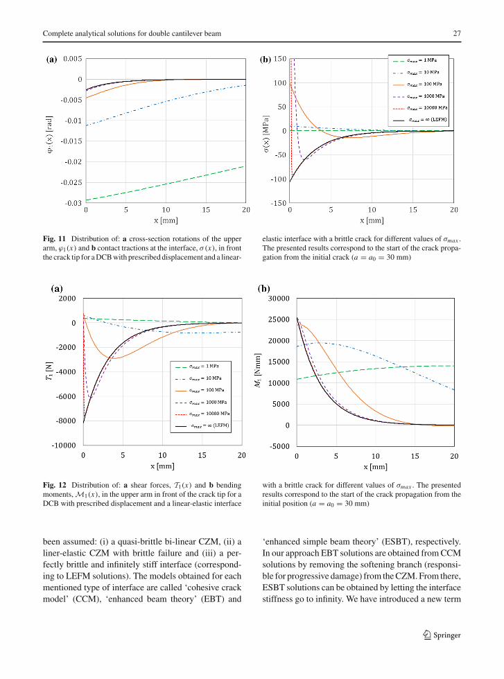
Complete analytical solutions for double cantilever beam 27

Fig. 11 Distribution of: a cross-section rotations of the upperarm, ϕ1(x) and b contact tractions at the interface, σ(x), in frontthe crack tip for aDCBwith prescribed displacement and a linear-

elastic interface with a brittle crack for different values of σmax .The presented results correspond to the start of the crack propa-gation from the initial crack (a = a0 = 30 mm)

Fig. 12 Distribution of: a shear forces, T1(x) and b bendingmoments,M1(x), in the upper arm in front of the crack tip for aDCB with prescribed displacement and a linear-elastic interface

with a brittle crack for different values of σmax . The presentedresults correspond to the start of the crack propagation from theinitial position (a = a0 = 30 mm)

been assumed: (i) a quasi-brittle bi-linear CZM, (ii) aliner-elastic CZM with brittle failure and (iii) a per-fectly brittle and infinitely stiff interface (correspond-ing to LEFM solutions). The models obtained for eachmentioned type of interface are called ‘cohesive crackmodel’ (CCM), ‘enhanced beam theory’ (EBT) and

‘enhanced simple beam theory’ (ESBT), respectively.In our approach EBT solutions are obtained fromCCMsolutions by removing the softening branch (responsi-ble for progressive damage) from theCZM.From there,ESBT solutions can be obtained by letting the interfacestiffness go to infinity. We have introduced a new term

123

28 L. Škec et al.

ESBT because we show that in the limit case of LEFM,EBTmodel does not correspond to ‘standard beam the-ory’ (SBT) model where the DCB arms act as if theywere clamped at the crack tip. In ESBT, the arms areallowed to rotate at and in front of the crack tip, which isdue exclusively to the shear deformability of the arms.This is why for the case when the arms are not shear-deformable (Euler–Bernoulli beam theory), ESBT cor-responds to SBT. We have also derived the CCM, EBTand SBT solutions for the case when Euler–Bernoullibeam theory is used to model the arms by simply let-ting the shear stiffness of the arms go to infinity. All thementioned solutions are derived for two different typesofDCB: onewith prescribed rotations andonewith pre-scribed displacement. The presented solutions allow usto easily compute the crack mouth opening displace-ment, applied load (moment or force), contact tractionsat the interface, displacement and rotations of the armsahead of the crack tip, and shear forces and bendingmoments in the arms for different DCB models.

The main novel contributions of the paper are asfollows:

1. The complete analytical solutions given in a uni-fied and compact form for DCBs (either with pre-scribed rotations or prescribed displacement) witha bi-linear CZM at the interface.

2. The complete analytical solutions given in a unifiedand compact form for DCBs (either with prescribedrotations or prescribed displacement) with linear-elastic interface with brittle failure. It is shown thatsuch EBT solutions, compared to CMM solutions,are very accurate in the phase of crack propagation.However, they are not able to capture the quasi-brittle behaviour before crack propagation.

3. The solutions for the limit case of LEFM which,in the case of Timoshenko beam theory (ESBT),show that at and in front of the crack tip thearms are allowed to rotate even if the interface isinfinitely stiff. This implies that Timoshenko beamtheory is, in a way, capable of capturing the realis-tic behaviour of the DCB in front of the crack tipand that the widely used assumption that in LEFMthe arms act as if they were clamped at the crack isnot necessary. However, we show that this assump-tion is still valid when the arms are modelled asEuler–Bernoulli beams.

4. An expression for the critical energy release rate,Gc, for a DCBwith prescribed displacement is pro-

posed, which, to the best of authors’ knowledge,is original. This expression, compared to the for-mula derived under the assumption that the armsare clamped at the crack tip, has an additional termwhich is dependent on the shear deformability ofthe arms and accounts for the rotations of the armsat the crack tip. If the arms are non-deformable inshear (Euler–Bernoulli beam theory), the expres-sion for Gc corresponds to the one obtained underthe assumptions that the arms are clamped at thecrack tip.

Future work will include the assessment of the accu-racy of the formula for Gc which in LEFM limit casetakes into account the rotations of the arms at the cracktip. Similar analyses have been already done by Bieland Stigh (2008) and the authors of the present work(Škec et al. 2018). Based on the data obtained from theexperiments or more sophisticated numerical models,our intention is to compare the accuracy of this formulawith formulae from BS ISO 25217:2009 (2009).

It is also worth noting that, using the approach pre-sented in this paper, obtaining the analytical solutionfor a DCB with trapezoidal CZM at the interface usingthe Timoshenko beam theory to model the arms shouldbe straight-forward and will also be covered in futurework.

Free software made available

All the results are implemented in a software appli-cation with a user-friendly graphic interface whereEuler–Bernoulli or Timoshenko beam theory for thearms and CCM, EBT or ESBT models for the inter-face can be selected. Results of the analysis can beplotted and exported. Because the computations arebased on the presented analytical solutions, the resultsin our software are obtained instantaneously, even ona regular laptop computer. The software is free andcan be downloaded at http://dx.doi.org/10.17633/rd.brunel.7223795.

Supplementary data

Supplementary material related to this article can befound online at http://dx.doi.org/10.17633/rd.brunel.7212218.

123

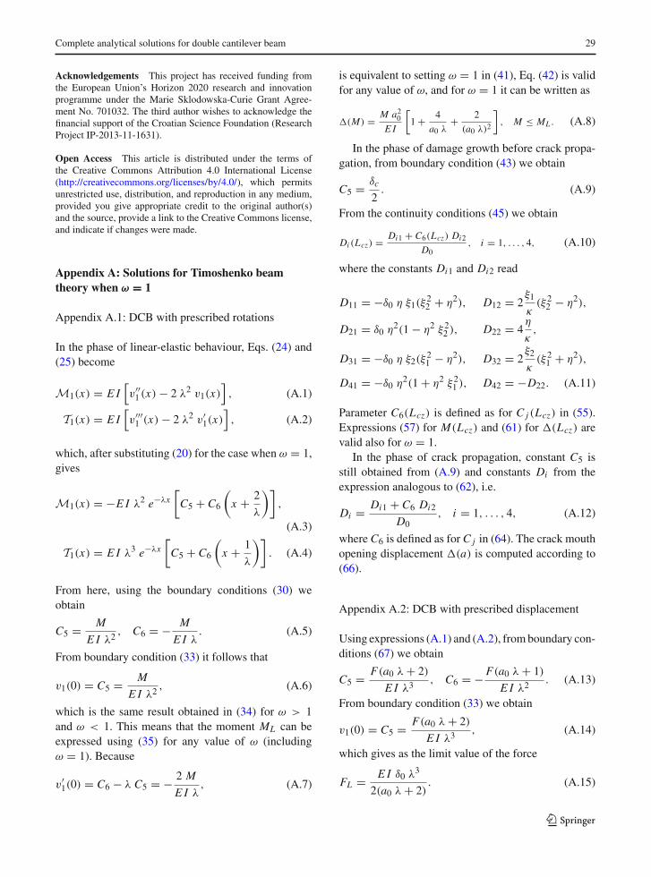
Complete analytical solutions for double cantilever beam 29

Acknowledgements This project has received funding fromthe European Union’s Horizon 2020 research and innovationprogramme under the Marie Sklodowska-Curie Grant Agree-ment No. 701032. The third author wishes to acknowledge thefinancial support of the Croatian Science Foundation (ResearchProject IP-2013-11-1631).

Open Access This article is distributed under the terms ofthe Creative Commons Attribution 4.0 International License(http://creativecommons.org/licenses/by/4.0/), which permitsunrestricted use, distribution, and reproduction in any medium,provided you give appropriate credit to the original author(s)and the source, provide a link to the Creative Commons license,and indicate if changes were made.

Appendix A: Solutions for Timoshenko beamtheory when ω = 1

Appendix A.1: DCB with prescribed rotations

In the phase of linear-elastic behaviour, Eqs. (24) and(25) become

M1(x) = E I[v′′1 (x) − 2 λ2 v1(x)

], (A.1)

T1(x) = E I[v′′′1 (x) − 2 λ2 v′

1(x)], (A.2)

which, after substituting (20) for the case when ω = 1,gives

M1(x) = −E I λ2 e−λx[

C5 + C6

(

x + 2

λ

)]

,

(A.3)

T1(x) = E I λ3 e−λx[

C5 + C6

(

x + 1

λ

)]

. (A.4)

From here, using the boundary conditions (30) weobtain

C5 = M

E I λ2, C6 = − M

E I λ. (A.5)

From boundary condition (33) it follows that

v1(0) = C5 = M

E I λ2, (A.6)

which is the same result obtained in (34) for ω > 1and ω < 1. This means that the moment ML can beexpressed using (35) for any value of ω (includingω = 1). Because

v′1(0) = C6 − λ C5 = − 2 M

E I λ, (A.7)

is equivalent to setting ω = 1 in (41), Eq. (42) is validfor any value of ω, and for ω = 1 it can be written as

�(M) = M a20E I

[

1 + 4

a0 λ+ 2

(a0 λ)2

]

, M ≤ ML . (A.8)

In the phase of damage growth before crack propa-gation, from boundary condition (43) we obtain

C5 = δc

2. (A.9)

From the continuity conditions (45) we obtain

Di (Lcz) = Di1 + C6(Lcz) Di2

D0, i = 1, . . . , 4, (A.10)

where the constants Di1 and Di2 read

D11 = −δ0 η ξ1(ξ22 + η2), D12 = 2

ξ1

κ(ξ22 − η2),

D21 = δ0 η2(1 − η2 ξ22 ), D22 = 4η

κ,

D31 = −δ0 η ξ2(ξ21 − η2), D32 = 2

ξ2

κ(ξ21 + η2),

D41 = −δ0 η2(1 + η2 ξ21 ), D42 = −D22. (A.11)

Parameter C6(Lcz) is defined as for C j (Lcz) in (55).Expressions (57) for M(Lcz) and (61) for �(Lcz) arevalid also for ω = 1.

In the phase of crack propagation, constant C5 isstill obtained from (A.9) and constants Di from theexpression analogous to (62), i.e.

Di = Di1 + C6 Di2

D0, i = 1, . . . , 4, (A.12)

where C6 is defined as for C j in (64). The crack mouthopening displacement �(a) is computed according to(66).

Appendix A.2: DCB with prescribed displacement

Using expressions (A.1) and (A.2), fromboundary con-ditions (67) we obtain

C5 = F(a0 λ + 2)

E I λ3, C6 = − F(a0 λ + 1)

E I λ2. (A.13)

From boundary condition (33) we obtain

v1(0) = C5 = F(a0 λ + 2)

E I λ3, (A.14)

which gives as the limit value of the force

FL = E I δ0 λ3

2(a0 λ + 2). (A.15)

123

30 L. Škec et al.

The latter result implies that Eq. (71) is valid also forthe case when ω = 1. Furthermore, (A.14) and

v′1(0) = − F(2 a0 λ + 3)

E I λ2(A.16)

show that expressions (70) and (76) are valid also forω = 1. Thus, the crack mouth opening can be com-puted according to (77) as

�(F) = 2 F a303 E I

[

1 + 6 (a0 λ + 1)2

(a0λ)3

]

, F ≤ FL . (A.17)

For the second phase of the solution we again obtain(A.9) and (A.10) from condition (43) and the continu-ity conditions (45), respectively. Constant C6(Lcz) isdefined as for C j (Lcz) in (81), where the definitions(A.11) for constants Di1 and Di2 (i = 1, . . . , 4) mustbe used.We can express F(Lcz) using (80) and�(Lcz)

using (83).For the phase of crack propagation we compute Di

(i = 1, . . . , 4) according to (A.12), where C6(Lcz) iscomputed asC j (Lcz) in (85)with definitions (A.11) forconstants Di1 and Di2 (i = 1, . . . , 4). Constant C5 isstill defined according to (A.9). Functions F(Lcz) anda(Lcz) are computed from (78) and (87), respectively.Finally, �(Lcz) can be computed from (88).

Appendix B: Solutions for Euler–Bernoulli beamtheory

In this section, we will assume that DCB arms areshear-undeformable by letting μ → ∞. This will sim-ply transform solutions for Timoshenko beam theorypresented in Sects. 3 and 4 into solutions for Euler–Bernoulli beam theory.

According to (9)2 and (10)2, in the limit of μ → ∞both ω and ψ tend to 0. This means that on the undam-aged part of the interface the solution will be definedas for the case when ω < 1 in Sect. 2.2.1. Setting ω =ψ = 0, from (15) and (22), respectively, we now obtain

ζ3 = ζ4 =√2

2, and ξ1 = ξ2 = 1. (B.1)

The displacements of the upper arm on the undam-aged and damaged part of the interface read

v1(x) = e−λE x [sin(λE x)C3

+ cos(λE x)C4] , for x ≥ 0, (B.2)

v2(x) = sin(κ x)D1 + cos(κ x)D2 + sinh(κ x)D3

+ cosh(κ x)D4 + δc

2, for x ∈ [−Lcz, 0], (B.3)

respectively, where λE = √2λ/2. Definitions (B.2)

and (B.3) are now used to solve the problems of a DCBwith either rotations or displacement prescribed.

Appendix B.1: DCB with prescribed rotations

The three-phase solution procedure reported in Sect. 3is followed. For the liner-elastic phase we have

C3 = −C4, C4 = M

E Iλ2= M

2 E I λ2E(B.4)

and

ML = E I δ0 λ2

2= E I δ0 λ2E . (B.5)

The crack mouth opening displacement in the linear-elastic phase can be expressed using (42) as

�(M) = M a20E I

(

1 + 1

a0 λE

)2

, M ≤ ML . (B.6)

For the phase of damage growth before crack prop-agation, we use (50) to determine constants Di (i =1, . . . , 4), where now C j (Lcz) = C3(Lcz). From (44)we know that

C4 = δ0

2. (B.7)

By taking into account (B.1), from (51) we get

D0 = 4, (B.8)

and from (53)

D11 = − δ0 ηE (1 + 2 η2E ), D12 =2 ηE (1 − 2 η2E ),

D21 = − 4 δ0 η4E , D22 =4 η2E ,

D31 = − δ0 ηE (1 − 2 η2E ), D32 =2 ηE (1 + 2 η2E ),

D41 =D21, D42 = − D22, (B.9)

where ηE = λE/κ . Constant C3(Lcz) is expressedfrom (55) for j = 3 and it reads

C3(Lcz) = −D21 sin(κ Lcz) + D11 cos(κ Lcz) + D41 sinh(κ Lcz) − D31 cosh(κ Lcz)

D22 sin(κ Lcz) + D12 cos(κ Lcz) + D42 sinh(κ Lcz) − D32 cosh(κ Lcz). (B.10)

Equations (57) and (48) give the solution for M(Lcz)

which is then used to numerically compute the value of

123

Complete analytical solutions for double cantilever beam 31

Lcz from Eq. (58) so that Mmax = M(Lcz). The crackmouth opening displacement in the second phase iscomputed from (61), where v2(Lcz) and v′

2(Lcz) areobtained from (B.3).

In the third phase we obtain constants Di (i =1, . . . , 4) from (62) by using expressions (B.8) and(B.9) for D0, Di1 and Di2 and assuming that nowC j = C3. Equation (64) now becomes

C3 = D11 sin(κ Lcz) − D21 cos(κ Lcz) + D31 sinh(κ Lcz) − D41 cosh(κ Lcz)

−D12 sin(κ Lcz) + D22 cos(κ Lcz) − D32 sinh(κ Lcz) + D42 cosh(κ Lcz). (B.11)

The crack mouth opening displacement in the phase ofcrack propagation is computed according to (66).

Appendix B.2: DCB with prescribed displacement

In the linear-elastic phase constants (69) for the solu-tion (B.2) become

C3 = − F a02 E I λ2E

, C4 = F(a0 λE + 1)

2 E Iλ3E. (B.12)

From (71) we obtain

FL = E I δ0 λ3E

1 + a0 λE. (B.13)

The crack mouth opening displacement is obtainedfrom (77) as

�(F) = 2F a303 E I

{

1 + 3

2(a0λE )3[2 a0 λE

+ 2(a0 λE )2 + 1]}

, F ≤ FL . (B.14)

In the second phase, we define Di (Lcz) (i =1, . . . , 4) according to (50), where we use (B.8) and(B.9) and assume that C j (Lcz) = C3(Lcz). The latteris defined according to (81) as

C3(Lcz) = β1 sin(κ Lcz) + β2 cos(κ Lcz) + β3 sinh(κ Lcz) + β4 cosh(κ Lcz)

β5 sin(κ Lcz) + β6 cos(κ Lcz) + β7 sinh(κ Lcz) + β8 cosh(κ Lcz), (B.15)

where

β1 = D11 + a0 κ D21, β2 = −D21 + a0 κ D11,

β3 = −D31 + a0 κ D41, β4 = D41 − a0 κ D31,

β5 = −D12 − a0 κ D22, β6 = D22 − a0 κ D12,

β7 = D32 − a0 κ D42, β8 = −D42 + a0 κ D32,

(B.16)

with constants Di1 and Di2 (i = 1, . . . , 4) definedin (B.9). F(Lcz) is computed according to (80), whereM(Lcz) is defined in (57). The limit value Lmax

cz is deter-mined from Eq. (58) which is solved numerically. Thecrack mouth opening displacement is computed from(83).

In the third phase we use (85) to express C3(Lcz) as

C3(Lcz) = D11 sin(κ Lcz) − D21 cos(κ Lcz) + D31 sinh(κ Lcz) − D41 cosh(κ Lcz)

−D12 sin(κ Lcz) + D22 cos(κ Lcz) − D32 sinh(κ Lcz) + D42 cosh(κ Lcz), (B.17)

where Di1 and Di2 (i = 1, . . . , 4) are defined in (B.9).Function F(Lcz) is obtained from condition (78) and(49), whereas a(Lcz) is expressed using (87). Finally,the crack mouth opening displacement for the thirdphase can be computed according to (88).

Appendix C: Euler–Bernoulli beam theory solu-tions for a DCB with linear-elastic interface withbrittle failure (EBT)

Appendix C.1: DCB with prescribed rotations

In the linear-elastic phase before crack propagationwe compute the crack mouth opening displacementaccording to (B.6), whereas for the crack propagationphase we have

123

32 L. Škec et al.

�(a) = Mmax a2

E I

(

1 + 1

a λE

)2

, a ≥ a0, (C.1)

where Mmax is defined in (93).

Appendix C.2: DCB with prescribed displacement

The crack mouth opening displacement in the linear-elastic phase before crack propagation is computedaccording to (B.14). The peak load, as defined in (95),now becomes

Fmax =√E I b Gc

a0 + 1λE

. (C.2)

In the crack propagation phase, the crack mouth open-ing displacement is computed as

�(a) = 2F(a) a3

3 E I

{

1 + 3

2(a λE )3[2 a λE

+2(a λE )2 + 1]}

, a ≥ a0, (C.3)

where according to (97) we now have

F(a) =√E I b Gc

a + 1λE

. (C.4)

Appendix D: LEFM solutions for a DCB usingEuler–Bernoulli beam theory (SBT)

Appendix D.1: DCB with prescribed rotations

Letting μ → ∞ in (105) and (106), or λE → ∞in (B.6) and (C.1), results in the following expressionsfor the crackmouth opening displacement when Euler–Bernoulli beam theory is used:

�(M) = M a20E I

,

before crack propagation (M ≤ Mmax ),

(D.1)

�(a) = Mmax a2

E I,

during crack propagation (a ≥ a0), (D.2)

where Mmax is defined in (93). In contrast to formu-lae (105) and (106), where Timoshenko beam theoryis used, from these expressions, it is obvious that forEuler–Bernoulli beam theory the arms of a DCB in thelimit case of LEFM indeed act as if they were clampedat the crack tip.

Appendix D.2: DCB with prescribed displacement

By letting μ → ∞ in (113) and (115), or λE → ∞ in(B.14) and (C.3), we can derive the expressions for thecrackmouth opening displacement for Euler–Bernoullibeam theory as

�(F) = 2 F a303 E I

,

before crack propagation (F ≤ Fmax ), (D.3)

�(a) = 2 F(a) a3

3 E I,

during crack propagation (a ≥ a0), (D.4)

where

Fmax =√E I b Gc

a0and F(a) =

√E I b Gc

a.

(D.5)

The last expression gives the widely used LEFM for-mula for Gc in the case of a DCB with prescribed dis-placement

Gc = F2 a2

b E I, (D.6)

where again, for the sake of simplicity, we replace F(a)

simply by F . By combining (D.4) and (D.6) we get

Gc = F2

b E I

(3 E I �

2 F

) 23 = 3

√

9 �2 F4

4 b3 E I. (D.7)

This formula requires the knowledge (experimentalmeasurement) of only � and F , whereas the knowl-edge of the crack length a is not relevant. Note thatexpression for Gc according to Timoshenko beam the-ory which requires the knowledge of only � and Fcan be derived, too, by combining (117) and (115), butthis procedure is less-straight forward and it requiressolving of a cubic equation. This result is not reportedfor the sake of simplicity and because in Sect. 7.2 wedemonstrate that sufficiently accurate calculation ofGc

can be accomplished using formula (D.7).

Appendix E: Expressions of v1, v′1, ϕ1, σ , T1 and

M1 for the limit case of LEFM

We already mentioned that for the limit case of LEFMδ0 = δc → 0 and σmax → ∞, which results in λ → ∞and ω → ∞. This means that only the solution for

123

Complete analytical solutions for double cantilever beam 33

v1(x) when ω > 1 (see (20)) is considered in the limitcase of LEFM, i.e.

v1(x) = e−λζ1x C1 + e−λζ2x C2. (E.1)

ConstantsC1 andC2 are defined according to (31) for aDCBwith prescribed rotations, or according to (68) fora DCB with prescribed displacement. In the followingsubsections we will present the limit (LEFM) values offunctions v1, v′

1, ϕ1, σ , T1 and M1 for both cases.

Appendix E.1: DCB with prescribed rotations

Substituting (31) for C1 and C2 in (E.1) results in

v1(x) = M

E I λ2

(e−λζ1x

1 − ζ 22

+ e−λζ2x

1 − ζ 21

)

= M

E I λ2(ζ1 − ζ2)

(ζ1 e

−λζ1x − ζ2 e−λζ2x

), (E.2)

where the relation ζ1ζ2 = 1 is used to simplify theexpression. If we introduce the following notation

ρ1 = ζ1/λ =√

χ +√

χ2 − 1/λ4, (E.3)

ρ2 = ζ2/λ =√

χ −√

χ2 − 1/λ4, (E.4)

where χ = E I/(2μAs), we can rewrite (E.2) as

v1(x) = M

E I λ2(ρ1 − ρ2)

(ρ1 e

−λ2ρ1x − ρ2 e−λ2ρ2x

). (E.5)

Multiplying (E.3) and (E.4) and because ζ1ζ2 = 1, onethen has that λ2ρ2 = 1/ρ1, so that we can write:

v1(x) = M

E I λ2(ρ1 − ρ2)

(ρ1 e

−λ2ρ1x − ρ2 e− x

ρ1

). (E.6)

Note that in the exponent of the second term inthe parenthesis we avoid λ2ρ2 and use 1/ρ1 insteadbecause

limλ→∞ ρ1 = √

2χ =√

E I

μAs, and lim

λ→∞ ρ2 = 0, (E.7)

show that the limit value of λ2ρ2, unlike 1/ρ1, is lessconvenient for computer implementation. From (E.6)it then follows that

limλ→∞ v1(x) = 0, for x ≥ 0. (E.8)

According to (89) we can write

σ(x) = σmax

δ0δ(x) = 2 σmax

δ0v1(x), (E.9)

which after substituting (E.6) and using definition (9)1for λ becomes

σ(x) =M

(λ2 ρ2

1 e−λ2ρ1x − e− x

ρ1

)

b(ρ21 − 1

λ2

) . (E.10)

Therefore, we have σ(0) = Mλ2/b andσ L(0) = lim

λ→∞ σ(0) = ∞, (E.11)

whereas

σ L(x) = limλ→∞ σ(x)

= −M μAs

b E Ie−

√μAsE I x

, for x > 0, (E.12)

from which it follows that

σ L(0+) = −M μAs

b E I. (E.13)

From (E.10) it can be shown that the interface stressprofile for finite values of λ starts from a positivevalue at x = 0, decreases to zero at a coordinate x =x0 = ln(ρ1/ρ2)/

[λ2(ρ1 − ρ2)

], continues decreasing

to a minimum, negative value, at a coordinate xmin =2x0, and then remains negative, but also increasesand approaches zero asymptotically for x → ∞. Forλ → ∞, x0 → 0 and xmin → 0. Stress profiles for dif-ferent values of λ are reported in Fig. 11b. Note that theintegral of the stress profile σ L(x) in (E.12) is finite:∫ ∞

0+σ L(x)dx = −M

b

√μAs

E I(E.14)

and therefore, for the vertical equilibrium to be satis-

fied the resultant F0 = b limc→0

c∫

0σ L(x)dx of the infinite

stress σ L(0) in (E.11) must be finite:

F0 + b∫ ∞

0+σ L (x)dx = 0 �⇒ F0 = M

√μAs

E I, (E.15)

where F0 is a tensile concentrated force at the cracktip pointing downwards. Hence, the LEFM-limit stressprofile, σ L , is not a proper function but a generalisedone, which is the sum of (E.12) and of F0/bmultipliedby a Dirac distribution D centred at zero:

σ L(x) = −M μAs

b E Ie−

√μAsE I x

+M

b

√μAs

E ID(x), for x ≥ 0. (E.16)

Thus, according to (5), we can define the distributionof loads on the upper layer in the limit case of LEFM as

qL(x) = −σ L(x) b = M μAs

E Ie−

√μAsE I x

123

34 L. Škec et al.

− M

√μAs

E ID(x), for x ≥ 0. (E.17)

Because T ′1 (x) = q(x), we can write

T L1 (x) =

∫

qL (x)dx + c1

= − M

√μAs

E Ie−

√μAsE I x − M

√μAs

E IH(x) + c1,(E.18)

where

H(x) ={0 for x = 0,1 for x > 0,

(E.19)

is Heaviside (step) function and c1 is an integrationconstant. Note that H(x) is dimensionless, whereasthe dimension of D(x) is the inverse of a length.Using the boundary condition T L

1 (0) = 0, we obtainc1 = F0 = M

√μAs/E I , so that

T L1 (x) = −M

√μAs

E I

[

e−√

μAsE I x

+ (H(x) − 1)] , for x ≥ 0, (E.20)

Because T1(x) = M′1(x), it follows that the distribu-

tion of bending moments on the upper layer for thelimit case of LEFM reads

ML1 (x) =

∫

T L1 (x)dx = Me−

√μAsE I x

−M

√μAs

E I

∫

(H(x) − 1)dx + c2, (E.21)

where c2 is an integration constants. Because∫(H(x)−

1)dx = 0 for any x ≥ 0, conditionML1 (0) = M gives

c2 = 0, and we finally have

ML1 (x) = Me−

√μAsE I x

, for x ≥ 0. (E.22)

Note that, as expected, T L1 (∞) = ML

1 (∞) = 0.From (E.6) we can obtain

v′1(x) = −

M(ρ21 e−λ2ρ1x − ρ2

2 e− x

ρ1

)

E I (ρ1 − ρ2), (E.23)

which gives

v′1(0) = −M(ρ1 + ρ2)

E I, and

v′L1 (0) = lim

λ→∞ v′1(0) = − M√

E I μAs. (E.24)

The value of v′1(x) for the limit case of LEFM can be

obtained from (E.23) as

v′L1 (x) = lim

λ→∞ v′1(x) = 0, for x > 0, (E.25)

which, because v′L1 (0) is defined in (E.24), shows that

the function v′L(x) has a discontinuity at the crack tip(x = 0), too. Thus, we can write

v′L1 (x) = M√

E I μAs(H(x) − 1), for x ≥ 0. (E.26)

Finally, from ϕ1(x) = v′1(x)+T1(x)/μAs for the limit

case of LEFM we can obtain

ϕL1 (x) = − M√

E I μAse−

√μAsE I x

, for x ≥ 0, (E.27)

which gives the rotation of the upper layer at the cracktip ϕL

1 (0) = −M/√E I μAs .

Appendix E.2: DCB with prescribed displacement

Substituting (68) in (E.1) gives

v1(x) = F

E I λ3(ζ1 − ζ2)

[ζ1(ζ1 + a0 λ)e−λζ1x

− ζ2(ζ2 + a0 λ)e−λζ2x], (E.28)

or

v1(x) = F

E I λ2(ρ1 − ρ2)

[ρ1(ρ1 + a0)e

−λ2ρ1x

− ρ2(ρ2 + a0)e− x

ρ1

]. (E.29)

Using (E.9) we can obtain

σ(x) = F

b (ρ1 − ρ2)

(ρ1 + a0

ρ2e−λ2ρ1x

− ρ2 + a0ρ1

e− x

ρ1

)

, (E.30)

from which it follows that

σ(0) = F λ2

b(a0 + ρ1 + ρ2) and

σ L(0) = limλ→∞ σ(0) = ∞, (E.31)

whereas

σ L(x) = limλ→∞ σ(x)

= − F a0 μAs

b E Ie−

√μAsE I x

, for x > 0, (E.32)

so that

σ L(0+) = − F a0 μAs

b E I. (E.33)

The interface stress profile is now very similar to theone defined in (E.12) for the case of a DCB with pre-scribed rotations. It can be shown that for (E.32) zerostress and minimum stress correspond to

123

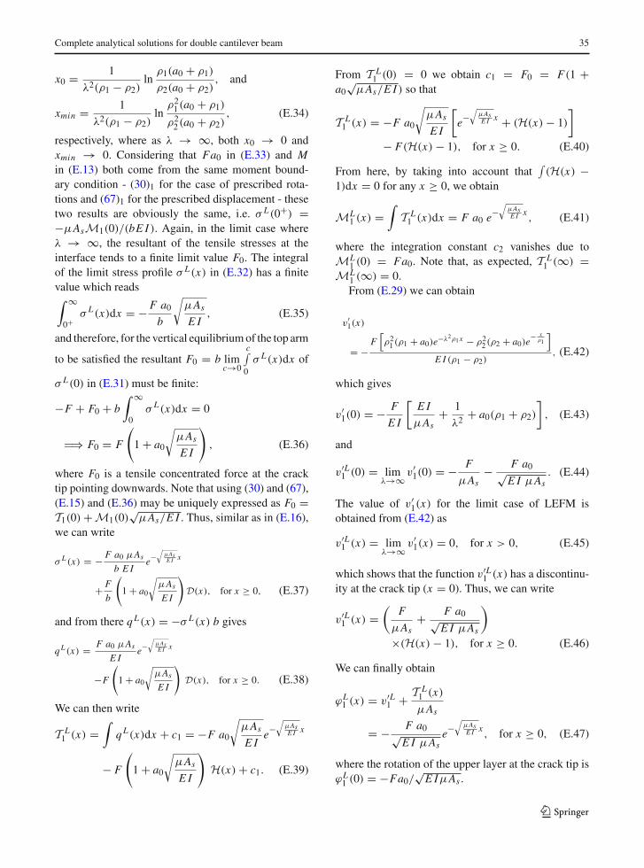
Complete analytical solutions for double cantilever beam 35

x0 = 1

λ2(ρ1 − ρ2)ln

ρ1(a0 + ρ1)

ρ2(a0 + ρ2), and

xmin = 1

λ2(ρ1 − ρ2)ln

ρ21 (a0 + ρ1)

ρ22 (a0 + ρ2)

, (E.34)

respectively, where as λ → ∞, both x0 → 0 andxmin → 0. Considering that Fa0 in (E.33) and Min (E.13) both come from the same moment bound-ary condition - (30)1 for the case of prescribed rota-tions and (67)1 for the prescribed displacement - thesetwo results are obviously the same, i.e. σ L(0+) =−μAsM1(0)/(bE I ). Again, in the limit case whereλ → ∞, the resultant of the tensile stresses at theinterface tends to a finite limit value F0. The integralof the limit stress profile σ L(x) in (E.32) has a finitevalue which reads∫ ∞

0+σ L(x)dx = − F a0

b

√μAs

E I, (E.35)

and therefore, for the vertical equilibriumof the top arm

to be satisfied the resultant F0 = b limc→0

c∫

0σ L(x)dx of

σ L(0) in (E.31) must be finite:

−F + F0 + b∫ ∞

0σ L(x)dx = 0

�⇒ F0 = F

(

1 + a0

√μAs

E I

)

, (E.36)

where F0 is a tensile concentrated force at the cracktip pointing downwards. Note that using (30) and (67),(E.15) and (E.36) may be uniquely expressed as F0 =T1(0) + M1(0)

√μAs/E I . Thus, similar as in (E.16),

we can write

σ L (x) = − F a0 μAs

b E Ie−

√μAsE I x

+ F

b

(

1 + a0

√μAs

E I

)

D(x), for x ≥ 0, (E.37)

and from there qL(x) = −σ L(x) b gives

qL (x) = F a0 μAs

E Ie−

√μAsE I x

−F

(

1 + a0

√μAs

E I

)

D(x), for x ≥ 0. (E.38)

We can then write

T L1 (x) =

∫

qL(x)dx + c1 = −F a0

√μAs

E Ie−

√μAsE I x

− F

(

1 + a0

√μAs

E I

)

H(x) + c1. (E.39)

From T L1 (0) = 0 we obtain c1 = F0 = F(1 +

a0√

μAs/E I ) so that

T L1 (x) = −F a0

√μAs

E I

[

e−√

μAsE I x + (H(x) − 1)

]

− F(H(x) − 1), for x ≥ 0. (E.40)

From here, by taking into account that∫(H(x) −

1)dx = 0 for any x ≥ 0, we obtain

ML1 (x) =

∫

T L1 (x)dx = F a0 e

−√

μAsE I x

, (E.41)

where the integration constant c2 vanishes due toML

1 (0) = Fa0. Note that, as expected, T L1 (∞) =

ML1 (∞) = 0.From (E.29) we can obtain

v′1(x)

= −F[ρ21 (ρ1 + a0)e−λ2ρ1x − ρ2

2 (ρ2 + a0)e− x

ρ1

]

E I (ρ1 − ρ2), (E.42)

which gives

v′1(0) = − F

E I

[E I

μAs+ 1

λ2+ a0(ρ1 + ρ2)

]

, (E.43)

and

v′L1 (0) = lim

λ→∞ v′1(0) = − F

μAs− F a0√

E I μAs. (E.44)

The value of v′1(x) for the limit case of LEFM is

obtained from (E.42) as

v′L1 (x) = lim

λ→∞ v′1(x) = 0, for x > 0, (E.45)

which shows that the function v′L1 (x) has a discontinu-

ity at the crack tip (x = 0). Thus, we can write

v′L1 (x) =

(F

μAs+ F a0√

E I μAs

)

×(H(x) − 1), for x ≥ 0. (E.46)

We can finally obtain

ϕL1 (x) = v′L

1 + T L1 (x)

μAs

= − F a0√E I μAs

e−√

μAsE I x

, for x ≥ 0, (E.47)

where the rotation of the upper layer at the crack tip isϕL1 (0) = −Fa0/

√E IμAs .

123

36 L. Škec et al.

Appendix E.3: Euler–Bernoulli beam theory

In the limit case of LEFM for Euler–Bernoulli beamtheory (μ → ∞) Eqs. (98)–(103) for a DCB with pre-scribed rotations become

vL1 (x) = v′L

1 (x) = ϕL1 (x) = T L

1 (x) = 0, (E.48)

σ L(x) = D(x), (E.49)

ML1 (x) = M(1 − H(x)). (E.50)

Equations (107)–(112) for a DCB with prescribed dis-placement become

vL1 (x) = v′L

1 (x) = ϕL1 (x) = 0, (E.51)

σ L(x) = D(x), (E.52)

T L1 (x) = F (1 − H(x)), (E.53)

ML1 (x) = F a0(1 − H(x)). (E.54)

These expressions confirm that the DCB arms do notdeform at and in front of the crack tip when theyare modelled as Euler–Bernoulli beams. Analogousexpressions for the phase of crack propagation couldbe obtained by substitutingM withMmax , F with F(a)

and a0 with a.

References

Alfano G, Crisfield MA (2001) Finite element interface modelsfor the delamination analysis of laminated composites:mechanical and computational issues. Int J NumerMethodsEng 50(7):1701–1736

ASTM D3433-99 (2012) Standard test method for fracturestrength in cleavage of adhesives in bonded metal joints.ASTM International (2012)

Barenblatt GI (1959) The formation of equilibrium cracks dur-ing brittle fracture—general ideas and hypothesis, axiallysymmetric cracks. J Appl Math Mech 23(3):622–636

Benbow JJ, Roesler FC (1957) Experiments on controlledfractures. Proc Phys Soc 70(B):201–211

Biel A, Stigh U (2008) Effects of constitutive parameterson the accuracy of measured fracture energy using theDCB-specimen. Eng Fract Mech 75:2968–2983

Blackman BRK, Kinloch AJ, Paraschi M, Teo WS (2003a)Measuring the mode I adhesive fracture energy, GIC , ofstructural adhesive joints: the results of an internationalround-robin. Int J Adhes Adhes 23:293–305

Blackman BRK, Hadavinia H, Kinloch AJ,Williams JG (2003b)The use of a cohesive zone model to study the fracture offibre composites and adhesively-bonded joints. Int J Fract119:25–46

BS ISO 25217:2009 (2009) Adhesives—determination of themode I adhesive fracture energy of structural adhesivejoints using double cantilever beam and tapered doublecantilever beam specimens. British Standard

de Morais AB (2013) Mode I cohesive zone model for delam-ination in composite beams. Eng Fract Mech 109:236–245

de Morais AB (2015) Analysis of the metal adhesively bondeddouble cantilever beam specimen. Int J Adhes Adhes61:8–14

de Moura MFSF, Campilho RDSG, Gonçalves JPM (2008)Crack equivalent concept applied to the fracture characteri-zation of bonded joints under pure mode I loading. ComposSci Technol 68:2224–2230

Dimitri R, Cornetti P, Mantic V, Trullo M, De Lorenzis L(2017) Mode-I debonding of a double cantilever beam: acomparison between cohesive crack modeling and finitefracture mechanics. Int J Solids Struct 124:57–72

Dugdale DS (1960) Yielding of steel sheets containing slits. JMech Phys Solids 8:100–104

Freiman SW, Mulville DR, Mast PW (1973) Crack propagationstudies in brittle materials. J Mater Sci 8:1527–1533

Gehlen PC, Popelar CH, Kanninen MF (1979) Modelingof dynamic crack propagation: I. validation of one-dimensional analysis. Int J Fract 15(3):281–294

Hillerborg A, Modéer M, Petersson PE (1976) Analysis ofcrack formation and crack growth in concrete by meansof fracture mechanics and finite elements. Cem Concr Res(Sec. 12.2) 6:773–782

Irwin GR (1956) Onset of fast crack propagation in highstrength steel and aluminuim alloys. Sagmore Res ConfProc 2:289–305

Kanninen MF (1973) An augmented double cantilever beammodel for studying crack propagation and arrest. Int J Fract9(1):83–92

Kanninen MF (1974) A dynamic analysis of unstable crackpropagation and arrest in the DCB test specimen. Int J Fract10(3):415–430

Park K, Paulino GH (2011) Cohesive zone models: a criticalreview of traction-separation relationships across fracturesurfaces. Appl Mech Rev 64:060802-1–060802-20

Rice JR (1968) A path independent integral and the approximateanalysis of strain concentration by notches and cracks. JAppl Mech 35:379–386

Ripling EJ, Mostovoy S, Corten HT (1971) Fracture mechan-ics: a tool for evaluating structural adhesives. J Adhes3(2):107–123

Shahani AR, Amini Fasakhodi MR (2010) Analytical modellingof dynamic fracture and crack arrest in DCB specimensunder fixed displacement conditions. Fatigue Fract EngMater Struct 33:436–451

Shahani AR, Forqani M (2004) Static and dynamic fracturemechanics analysis of a DCB specimen considering sheardeformation effects. Int J Solids Struct 41:3793–3807

Škec L, Jelenic G (2017) Geometrically non-linear multi-layerbeam with interconnection allowing for mixed-modedelamination. Eng Fract Mech 169:1–17

Škec L, Jelenic G, Lustig N (2015) Mixed-mode delaminationin 2D layered beam finite elements. Int J Numer MethodsEng 104:767–788

123

Complete analytical solutions for double cantilever beam 37

Škec L, Alfano G, Jelenic G (2018) On Gc, Jc and the character-isation of the mode-I fracture resistance in delamination oradhesive debonding. Int J Solids Struct 144–145:100–122

Sørensen BF, Brethe P, Skov-Hansen P (1996) Controlled crackgrowth in ceramics: the DCB specimen loaded with puremoments. J Eur Ceram Soc 16:1021–1025

Stigh U (1988) Damage and crack growth anlysis of the doublecantilever beam specimen. Int J Fract 37:R13–R18

Suo Z, Bao G, Fan B (1992) Delamination R-curve phenomenadue to damage. J Mech Phys Solids 40(1):1–16

Williams JG (1989) End corrections for orthotropic DCBspecimens. Compos Sci Technol 35:367–376

Publisher’s Note Springer Nature remains neutral with regardto jurisdictional claims in published maps and institutional affil-iations.

123