compilation 2011 static analysis johnni winther michael i. schwartzbach aarhus university
TRANSCRIPT

Compilation 2011Compilation 2011
Static AnalysisStatic Analysis
Johnni WintherMichael I. Schwartzbach
Aarhus University

2Static Analysis
Interesting QuestionsInteresting Questions
Is every statement reachable? Does every non-void method return a value? Will local variables definitely be assigned before
they are read? Will the current value of a variable ever be read? ... How much heap space will the program need? Does the program always terminate? Will the output always be correct?

3Static Analysis
Rice’s TheoremRice’s Theorem
Theorem 11.9 (Martin p. 420)
If R is a property of languages that is satisfied by some but not all recursively enumerable languages then the decision problem
PR: Given a TM T, does L(T) have property R?
is unsolvable.

4Static Analysis
Rice’s Theorem ExplainedRice’s Theorem Explained
Theorem 11.9 (Martin, p. 420)
"Every non-trivial question about the behavior of a
program is undecidable."

5Static Analysis
Static AnalysisStatic Analysis
Static analysis provides approximate answers to non-trivial questions about programs
The approximation is conservative, meaning that the answers only err to one side
Compilers spend most of their time performing static analysis so they may:• understand the semantics of programs• provide safety guarantees• generate efficient code

6Static Analysis
Conservative ApproximationConservative Approximation
A typical scenario for a boolean property:• if the analysis says yes, the property definitely holds• if it says no, the property may or may not hold• only the yes answer will help the compiler• a trivial analysis will say no always• the engineering challenge is to say yes often enough
For other kinds of properties, the notion of approximation may be more subtle

7Static Analysis
A Range of Static AnalysesA Range of Static Analyses
Static analysis may take place:• at the source code level• at some intermediate level• at the machine code level
Static analysis may look at:• statement blocks only• an entire method (intraprocedural)• the whole program (interprocedural)
The precision and cost both rise as we include more information

8Static Analysis
The Phases of GCC (1/2)The Phases of GCC (1/2)
Parsing
Tree optimization
RTL generation
Sibling call optimization
Jump optimization
Register scan
Jump threading
Common subexpression elimination
Loop optimizations
Jump bypassing
Data flow analysis
Instruction combination
If-conversion
Register movement
Instruction scheduling
Register allocation
Basic block reordering
Delayed branch scheduling
Branch shortening
Assembly output
Debugging output
9Static Analysis
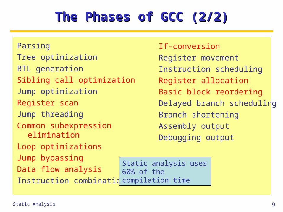
The Phases of GCC (2/2)The Phases of GCC (2/2)
Parsing
Tree optimization
RTL generation
Sibling call optimization
Jump optimization
Register scan
Jump threading
Common subexpression elimination
Loop optimizations
Jump bypassing
Data flow analysis
Instruction combination
If-conversion
Register movement
Instruction scheduling
Register allocation
Basic block reordering
Delayed branch scheduling
Branch shortening
Assembly output
Debugging output
Static analysis uses 60% of the compilation time
10Static Analysis
Reachability AnalysisReachability Analysis
Java requires two reachability guarantees:• all statements must be reachable (avoid dead code)• all non-void methods must return a value
These are non-trivial properties and thus they are undecidable
But a static analysis may provide conservative approximations
To ensure that different compilers accept the same programs, the Java language specification mandates a specific static analysis

11Static Analysis
Constraint-Based AnalysisConstraint-Based Analysis
For every node S that represents a statement in the AST, we define two boolean properties:• C[[S]] denotes that S may complete normally• R[[S]] denotes that S is possibly reachable
A statement may only complete if it is reachable
For each syntactic kind of statement, we generate constraints that relate C[[...]] and R[[...]]

12Static Analysis
Information FlowInformation Flow
The values of R[[...]] are inherited The values of C[[...]] are synthesized
AST
R C
13Static Analysis
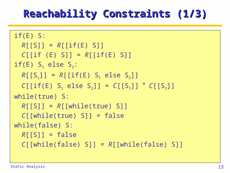
Reachability Constraints (1/3)Reachability Constraints (1/3)
if(E) S:
R[[S]] = R[[if(E) S]]
C[[if (E) S]] = R[[if(E) S]]
if(E) S1 else S2:
R[[Si]] = R[[if(E) S1 else S2]]
C[[if(E) S1 else S2]] = C[[S1]] C[[S2]]
while(true) S:
R[[S]] = R[[while(true) S]]
C[[while(true) S]] = false
while(false) S:
R[[S]] = false
C[[while(false) S]] = R[[while(false) S]]

14Static Analysis
Reachability Constraints (2/3)Reachability Constraints (2/3)
while(E) S:
R[[S]] = R[[while(E) S]]
C[[while(E) S]] = R[[while(E) S]]
return:
C[[return]] = false
return E:
C[[return E]] = false
throw E:
C[[throw E]] = false
{σ x; S}:
R[[S]] = R[[{σ x; S}]]
C[[{σ x; S}]] = C[[S]]

15Static Analysis
Reachability Constraints (3/3)Reachability Constraints (3/3)
S1S2:
R[[S1]] = R[[S1S2]]
R[[S2]] = C[[S1]]
C[[S1S2]] = C[[S2]]
for any simple statement S:
C[[S]] = R[[S]]
for any method or constructor body {S}:
R[[S]] = true

16Static Analysis
Exploiting the InformationExploiting the Information
For any statement S where R[[S]] = false:
unreachable statement
For any non-void method with body {S} where C[[S]] = true:
missing return statement
These guarantees are sound but conservative

17Static Analysis
ApproximationsApproximations
C[[S]] may be true too often:some unfair missing return errors may occur
if (b) return 17;
if (!b) return 42;
R[[S]] may be true too often:some dead code is not detected
if (b==!b) { ... }

18Static Analysis
Definite Assignment AnalysisDefinite Assignment Analysis
Java requires that a local variable is assigned before its value is used
This is a non-trivial property and thus it is undecidable
But a static analysis may provide a conservative approximation
To ensure that different compilers accept the same programs, the Java language specification mandates a specific static analysis
19Static Analysis
Constraint-Based AnalysisConstraint-Based Analysis
For every node S that represents a statement in the AST, we define some set-valued properties:• B[[S]] denotes the variables that are definitely
assigned before S is executed• A[[S]] denotes the variables that are definitely
assigned after S is executed
For every node E that represents an expression in the AST, we similarly define B[[E]] and A[[E]]

20Static Analysis
Increased PrecisionIncreased Precision
To handle cases such as: { int k;
if (a>0 && (k=System.in.read())>0) System.out.print(k);
}
we also use two refinements of A[[...]]:• At[[E]] which assumes that E evaluates to true
• Af[[E]] which assumes that E evaluates to false

21Static Analysis
Information FlowInformation Flow
The values of B[[...]] are inherited The values of A[[...]], At[[....]] and Af[[...]] are
synthesized
AST
B A, At, Af

22Static Analysis
Definite Assignment Constraints (1/7)Definite Assignment Constraints (1/7)
if(E) S:
B[[E]] = B[[if(E) S]]
B[[S]] = At[[E]]
A[[if(E) S]] = A[[S]] Af[[E]]
if(E) S1 else S2:
B[[E]] = B[[if(E) S1 else S2]]
B[[S1]] = At[[E]]
B[[S2]] = Af[[E]]
A[[if(E) S1 else S2]] = A[[S1]] A[[S2]]

23Static Analysis
Definite Assignment Constraints (2/7)Definite Assignment Constraints (2/7)
while(E) S:
B[[E]] = B[[while(E) S]]
B[[S]] = At[[E]]
A[[while(E) S]] = Af[[E]]
return:
A[[return]] = return E:
B[[E]] = B[[return E]]
A[[return E]] = throw E:
B[[E]] = B[[throw E]]
A[[throw E]] =
the set of all variables in scope

24Static Analysis
Definite Assignment Constraints (3/7)Definite Assignment Constraints (3/7)
E;:
B[[E]] = B[[E;]]
A[[E;]] = A[[E]]
{σ x=E; S}:
B[[E]] = B[[{σ x=E; S}]]
B[[S]] = A[[E]] {x}
A[[{σ x=E; S}]] = A[[S]]
{σ x; S}:
B[[S]] = B[[{σ x; S}]]
A[[{σ x; S}]] = A[[S]]

25Static Analysis
Definite Assignment Constraints (4/7)Definite Assignment Constraints (4/7)
S1S2:
B[[S1]] = B[[S1S2]]
B[[S2]] = A[[S1]]
A[[S1S2]] = A[[S2]]
x = E:
B[[E]] = B[[x = E]]
A[[x = E]] = A[[E]] {x}
x[E1] = E2:
B[[E1]] = B[[x[E1] = E2]]
B[[E2]] = A[[E1]]
A[[x[E1] = E2]] = A[[E2]]

26Static Analysis
Definite Assignment Constraints (5/7)Definite Assignment Constraints (5/7)
true:
At[[true]] = B[[true]]
Af[[true]] =
A[[true]] = B[[true]]
false:
At[[false]] =
Af[[false]] = B[[false]]
A[[false]] = B[[false]]
!E:
B[[E]] = B[[!E]] Af[[!E]] = At[[E]]
A[[!E]] = A[[E]] At[[!E]] = Af[[E]]

27Static Analysis
Definite Assignment Constraints (6/7)Definite Assignment Constraints (6/7)
E1 && E2:
B[[E1]] = B[[E1 && E2]]
B[[E2]] = At[[E1]]
At[[E1 && E2]] = At[[E2]]
Af[[E1 && E2]] = Af[[E1]] Af[[E2]]
A[[E1 && E2]] = At[[E1 && E2]] Af[[E1 && E2]]
E1 || E2:
B[[E1]] = B[[E1 || E2]]
B[[E2]] = Af[[E1]]
At[[E1 || E2]] = At[[E1]] At[[E2]]
Af[[E1 || E2]] = Af[[E2]]
A[[E1 || E2]] = At[[E1 || E2]] Af[[E1 || E2]]

28Static Analysis
Definite Assignment Constraints (7/7)Definite Assignment Constraints (7/7)
EXP(E1,...,Ek): (any other expression with subexpressions)
B[[E1]] = B[[EXP(E1,...,Ek)]]
B[[Ei+1]] = A[[Ei]]
A[[EXP(E1,...,Ek)]] = A[[Ek]]
When not specified otherwise:
At[[E]] = Af[[E]] = A[[E]]

29Static Analysis
Exploiting the InformationExploiting the Information
For every expression E of the form:• x• x++• x--• x[E']
where xB[[E]]:
variable might not have been initialized

30Static Analysis
ApproximationApproximation
A[[...]] and B[[...]] may be too small:
some unfair uninitialized variable errors may occur
{ int x;
if (b) x = 17;
if (!b) x = 42
System.out.print(x);
}

31Static Analysis
A Simpler GuaranteeA Simpler Guarantee
In Joos 1, definite assignment is guaranteed by:• requiring initializers for all local declarations• forbidding a local variable to appear in its own initializer
This is an even coarser approximation:
{ int x = (x=1)+42;
System.out.print(x)
}

32Static Analysis
Flow-Sensitive AnalysisFlow-Sensitive Analysis
The analyses for:• reachability• definite assignment
may simply be computed by traversing the AST
Other analyses are defined on the control flow graph of a program and require more complex techniques

33Static Analysis
Motivation: Register OptimizationMotivation: Register Optimization
For native code, we may want to optimize the use of registers:
mov 1,R3 mov 1,R1
mov R3,R1
This optimization is only sound if the value in R3 is not used in the future

34Static Analysis
Motivation: Register SpillsMotivation: Register Spills
When pushing a new frame, we write back all variables from registers to memory
It would be better to only write back those registers whose values may be used in the future
cba
yx
R1
R2
R3

35Static Analysis
LivenessLiveness
In both examples, we need to know if the value of some register Ri might be read in the future
If so, it is called live (and otherwise dead) Exact liveness is of course undecidable
A static analysis may conservatively approximate liveness at each program point
A trivial analysis thinks everything is live A superior analysis identifies more dead registers

36Static Analysis
Liveness AnalysisLiveness Analysis
For every program point Si we define the following set-valued properties:• B[[Si]] denotes the set of registers that are possibly
live before Si
• A[[Si]] denotes the set of registers that are possibly live after Si
For every program point we generate a constraint that relates A[[...]] and B[[...]] for neighboring program points
We no longer just use the AST...

37Static Analysis
TerminologyTerminology
succ(Si) denotes the set of program points to which execution may continue (by falling through or jumping)
uses(Si) denotes the set of registers that Si reads
defs(Si) denotes the set of registers that Si writes

38Static Analysis
A Tiny ExampleA Tiny Example
uses(Si) defs(Si) succ(Si)
S1: mov 3,R1 {} {R1} {S2}
S2: mov 4,R2 {} {R2} {S3}
S3: add R1,R2,R3 {R1,R2} {R3} {S4}
S4: mov R3,R0 {R3} {R0} {S5}
S5: return {R0} {} {}

39Static Analysis
Dataflow ConstraintsDataflow Constraints
For every program point Si we have:
B[[Si]] = uses(Si) (A[[Si]] \ defs(Si))
A[[Si]] = B[[x]]
xsucc(Si)
A cyclic control flow graph will generate a cyclic collection of constraints

40Static Analysis
Dataflow ExampleDataflow Example
S7: add R1,R2,R3
S8S9
S17
B[[S8]]={R4}B[[S9]]={R1}
B[[S17]]={R3}
B[[S7]]={R1,R2}({R4,R1,R3}\{R3})={R1,R2,R4}

41Static Analysis
A Small Example A Small Example
{ int i, even, odd, sum;
i = 1;
even = 0;
odd = 0;
sum = 0;
while (i < 10) {
if (i%2 == 0) even = even+i;
else odd = odd+i;
sum = sum+i;
i++;
}
}

42Static Analysis
Generated Native CodeGenerated Native Code
mov 1,R1 // R1 is i
mov 0,R2 // R2 is even
mov 0,R3 // R3 is odd
mov 0,R4 // R4 is sum
loop: andcc R1,1,R5 // R5 = R1 & 1
cmp R5,0
bne else // if R5!=0 goto else
add R2,R1,R2 // R2 = R2+R1
b endif
else: add R3,R1,R3 // R3 = R3+R1
endif: add R4,R1,R4 // R4 = R4+R1
add R1,1,R1 // R1 = R1+1
cmp R1,9
ble loop // if i<=9 goto loop

43Static Analysis
The Control Flow GraphThe Control Flow Graph
S5: andcc R1,1,R5
S1: mov 1,R1 S6: cmp R5,0
S8: add R2,R1,R2
S2: mov 0,R2 S7: bne S9 S10: add R4,R1,R4
S9: add R3,R1,R3
S3: mov 0,R3 S11: add R1,1,R1
S4: mov 0,R4 S12: cmp R1,9
S13: ble S5

44Static Analysis
Cyclic ConstraintsCyclic Constraints
B[[S1]] = f1(B[[S2]])
B[[S2]] = f2(B[[S3]])
B[[S3]] = f3(B[[S4]])
B[[S4]] = f4(B[[S5]])
B[[S5]] = f5(B[[S6]])
B[[S6]] = f6(B[[S7]])
B[[S7]] = f7(B[[S8]],B[[S9]])
B[[S8]] = f8(B[[S10]])
B[[S9]] = f9(B[[S10]])
B[[S10]] = f10(B[[S11]])
B[[S11]] = f11(B[[S12]])
B[[S12]] = f12(B[[S13]])
B[[S13]] = f13(B[[S5]])
where the fi(...) functions express the local constraints

45Static Analysis
Fixed-Point SolutionsFixed-Point Solutions
Reminder: x is a fixed point of a function f iff f(x)=x Define = (, , , , , , , , , , , ) Define R = {R0,R1,R2,R3,R4,R5}, (R) = Powerset of R Define F: (R)13→ (R)13 as:
F(X1,X2,X3,X4,X5,X6,X7,X8,X9,X10,X11,X12,X13) =
(f1(X2),f2(X3),f3(X4),f4(X5),f5(X6),f6(X7),f7(X8,X9),
f8(X9),f9(X10),f10(X11),f11(X12),f12(X13),f13(X5))
A solution is now a fixed point X(R)13 such that F(X)=X The least fixed point is computed as a Kleene iteration:
Fn()
for some n0

46Static Analysis
Computing the Least Fixed Point (1/3)Computing the Least Fixed Point (1/3)
F() F2 () F3 ()
S1 {} {} {} {}
S2 {} {} {} {}
S3 {} {} {} {R1}
S4 {} {} {R1} {R1}
S5 {} {R1} {R1} {R1}
S6 {} {R5} {R5} {R1,R2,R3,R5}
S7 {} {} {R1,R2,R3} {R1,R2,R3,R4}
S8 {} {R1,R2} {R1,R2,R4} {R1,R2,R4}
S9 {} {R1,R3} {R1,R3,R4} {R1,R3,R4}
S10 {} {R1,R4} {R1,R4} {R1,R4}
S11 {} {R1} {R1} {R1}
S12 {} {R1} {R1} {R1}
S13 {} {R1} {R1} {R1}

47Static Analysis
Computing the Least Fixed Point (2/3)Computing the Least Fixed Point (2/3)
F4 () F5() F6()
S1 {} {} {}
S2 {R1} {R1} {R1}
S3 {R1} {R1} {R1,R2}
S4 {R1} {R1,R2,R3} {R1,R2,R3}
S5 {R1,R2,R3} {R1,R2,R3,R4} {R1,R2,R3,R4}
S6 {R1,R2,R3,R4,R5} {R1,R2,R3,R4,R5}{R1,R2,R3,R4,R5}
S7 {R1,R2,R3,R4} {R1,R2,R3,R4} {R1,R2,R3,R4}
S8 {R1,R2,R4} {R1,R2,R4} {R1,R2,R4}
S9 {R1,R3,R4} {R1,R3,R4} {R1,R3,R4}
S10 {R1,R4} {R1,R4} {R1,R4}
S11 {R1} {R1} {R1,R2,R3}
S12 {R1} {R1,R2,R3} {R1,R2,R3,R4}
S13 {R1,R2,R3} {R1,R2,R3,R4} {R1,R2,R3,R4}
48Static Analysis
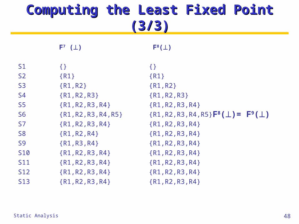
Computing the Least Fixed Point (3/3)Computing the Least Fixed Point (3/3)
F7 () F8()
S1 {} {}
S2 {R1} {R1}
S3 {R1,R2} {R1,R2}
S4 {R1,R2,R3} {R1,R2,R3}
S5 {R1,R2,R3,R4} {R1,R2,R3,R4}
S6 {R1,R2,R3,R4,R5} {R1,R2,R3,R4,R5}
S7 {R1,R2,R3,R4} {R1,R2,R3,R4}
S8 {R1,R2,R4} {R1,R2,R3,R4}
S9 {R1,R3,R4} {R1,R2,R3,R4}
S10 {R1,R2,R3,R4} {R1,R2,R3,R4}
S11 {R1,R2,R3,R4} {R1,R2,R3,R4}
S12 {R1,R2,R3,R4} {R1,R2,R3,R4}
S13 {R1,R2,R3,R4} {R1,R2,R3,R4}
F8()= F9()

49Static Analysis
Background: Why does this work?Background: Why does this work?
(R), the powerset of R, forms a lattice: It is a partial order, i.e., it is
• reflexive: S S
• transitive: if S1S2 and S2S3 then S1 S3
• anti-symmetric: if S1S2 and S2S1 then S1=S2
It has a least element () and a greatest element (R) Any two elements have a join S1S2 and a meet S1S2
Fixed point theorem: In a finite lattice L a monotone function F: LL has a unique least fixed point:
Fn() computable by Kleene iteration
n0

50Static Analysis
Application: Register AllocationApplication: Register Allocation
Variables that are never live at the same time may share the same register
Create a graph of variables where edges indicate simultaneous liveness:
Register allocation is done by finding a minimal graph coloring and assigning a register to each color: {{a,d,f}, {b,e}, {c}}
a
b
c
d
e
f