competitive applications - wiley.com · 409 competitive markets: applications 10.1 the invisible...
TRANSCRIPT

409
CompetitiveMarkets:
Applications
10.1 THE INVISIBLE HAND
10.2 IMPACT OF AN EXCISE TAX
Incidence of a TaxEXAMPLE 10.1 Gasoline Taxes
10.3 SUBSIDIES
10.4 PRICE CEILINGS (MAXIMUM PRICEREGULATION)
EXAMPLE 10.2 Scalping Super Bowl Tickets on the InternetEXAMPLE 10.3 Price Ceilings in the Market for
Natural Gas
10.5 PRICE FLOORS (MINIMUM PRICEREGULATION)
EXAMPLE 10.4 Unintended Consequences of Price Regulationin Airline Markets
10.6 PRODUCTION QUOTAS
EXAMPLE 10.5 Quotas for Taxi Cabs
10.7 OTHER PRICE SUPPORTS
EXAMPLE 10.6 Dumping
10.8 IMPORT TARIFFS AND QUOTAS
Chapter SummaryReview QuestionsProblems
10C H A P T E R
7784d_c10_409-461 5/23/01 6:48 AM Page 409

C H A P T E R P R E V I E WC H A P T E R P R E V I E W
Other programs have supportedprices for other commodities. For example, the government has sup-ported the price of peanuts by establishing “poundage quotas,” lim-iting the quantity of edible peanutsthat a farmer could sell. For manyyears domestic sugar producers haverelied on restrictive import quotas toraise sugar prices in the United States.The government has also supportedtobacco prices by restricting produc-tion to certain farms, and by limitingthe amounts that those farms couldproduce.
Acreage limitation programs, sub-sidies, and import and productionquotas are all forms of governmentintervention. In this chapter we willlearn how to analyze the conse-quences of government interventionin perfectly competitive markets. Sincethere are many small consumers and
producers of agriculturalcommodities, agriculturalmarkets have the structuralfeatures of perfect competi-tion. Absent price supports,the forces of supply and demand would lead to acompetitive equilibrium andan economically efficient allocation of agricultural re-sources.
We will learn how pro-grams of government inter-vention move the marketaway from a competitiveequilibrium, creating “dis-tortions” in the market aseconomic resources are re-allocated. We will also findthat intervention typicallymakes some people betteroff, while leaving othersworse off, helping us to un-derstand how the lines fordebates over public policyare drawn. For example,farmers who benefit fromprice supports often organ-ize themselves into a tightlyfocused interest group thatfights hard to retain the
ment expenditures on agriculturalprograms like the ones describedhere were more than $140 billion.
Price support programs can takemany forms. For example, under“acreage limitation programs” wheator feed grain farmers agree to restrictthe number of acres they plant. Inexchange, the government gives thefarmers an option to sell their cropsto the government at a guaranteedprice. Farmers are not required to sellhis crop to the government, andwould not do so if the market priceexceeds the guaranteed price. But afarmer will take the option to sell tothe government if the market priceis lower than the guaranteed price.Further, because an acreage limita-tion program reduces the amount ofthe crop on the market, the marketprice is higher than it otherwisewould be.
Price and income support pro- grams are commonplace in theworld. In the United States majoragricultural programs have beenaround since the 1930s. Governmentexpenditures on these programs haveranged in the billions of dollars an-nually, especially prior to 1996, whenCongress passed a major farm billthat eliminated or reduced many ofthe program benefits. HistoricallyCongress has required the Depart-ment of Agriculture to support theprices of about twenty commodities,including sugar (sugar cane andbeets), cotton, rice, feed grains (in-cluding corn, barley oats, rye, andsorghum), peanuts, wheat, tobacco,milk, soybeans and various types ofoil seeds (such as sunflower seed,mustard seed). During the fiscal yearsbetween 1983 and 1992, govern-
7784d_c10_409-461 5/23/01 6:48 AM Page 410
government programs, while someconsumer groups and taxpayers mayoppose the programs.
In this chapter we will analyze sev-eral forms of government interven-tion:
• Imposing excise taxes• Granting subsidies to producers• Regulating the maximum price
producers may charge• Regulating the minimum price
producers may charge• Setting quotas limiting the
amount that may be producedin a market
• Imposing tariffs or quotas onimports
Before we begin, note some im-portant points as we study the effectsof government intervention. In thischapter, we will use a partial equi-librium approach, usually focusingon only a single market. For example,we may examine the effect of rentcontrols on the market for housing.A partial equilibrium approach willnot allow us to ask how rent controlsaffect prices in other markets, includ-ing the market for housing that is notrented, and the markets for furniture,automobiles, and computers. To ex-amine how a change in one marketaffects all markets simultaneously, wewould need to employ a generalequilibrium model. A general equi-librium analysis determines the equi-librium prices and quantities in allmarkets simultaneously. We will in-troduce you to this more complexform of analysis in Chapter 16. The
conclusions we draw from a partialequilibrium analysis may not be thesame as those found with a generalequilibrium approach. Nevertheless,a partial equilibrium framework canoften be used to provide importantinsights about the primary effects ofgovernment intervention.
In this chapter we examine mar-kets that would be perfectly compet-itive absent government interven-tion. As we observed in Chapter 9, ina competitive market all producersand consumers are fragmented, thatis, they are so small in the market thatthey behave as price takers. If deci-sion makers have the ability to influ-ence the price in the market, we can-not use supply and demand analysis.Instead, we would need to apply anappropriate model of market power,such as the ones discussed in Chap-ters 11–14.
As we also learned in Chapter 9,in a perfectly competitive marketconsumers have perfect informationabout the nature of the product be-ing provided, as well as the price of the product. Sometimes govern-ments intervene in markets becauseconsumers are unable to gatherenough information about the prod-ucts in the market. For example, thehealth care sector would seem tohave a competitive structure, withmany providers and consumers ofhealth care services. Yet health careproducts, including medication andmedical procedures, can be so com-plex that the average consumer findsit difficult to make informed choices.Government intervention in this sec-tor is often designed to protect
consumers in such a complicatedmarket.
In perfectly competitive marketsthere are no externalities. Externali-ties are present in a market if the ac-tions of either consumers or produc-ers lead to costs or benefits that arenot reflected in the price of the prod-uct in that market. For example, aproduction externality will be presentif a producer pollutes the environ-ment. Pollution creates a social costthat might be ignored by a producerabsent government intervention. Aconsumption externality exists whenthe action of an individual consumerimposes costs on, or leads to benefitsfor, other consumers. For example,zoning ordinances in housing mar-kets are often intended to ensure thatconsumers of housing do not under-take activities that reduce the valueof property owned by others in aneighborhood. In this chapter we donot consider the effects of externali-ties; instead, we will address them inChapter 17.
Finally, throughout this chapterwe use consumer surplus to measurehow much better off or worse off aconsumer is when intervention af-fects the price in the market. As weshowed in Chapter 5, consumer sur-plus may not always be a good wayto measure the impact of a pricechange on a consumer. For somegoods (for example, for goods withlarge income effects), it may be im-portant to measure the effects ofprice changes on consumers by ex-amining compensating or equivalentvariations instead of using consumersurplus. �
C H A P T E R P R E V I E W
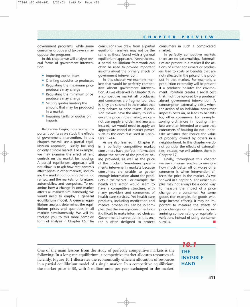
One of the main lessons from the study of perfectly competitive markets is thefollowing: In a long run equilibrium, a competitive market allocates resources ef-ficiently. Figure 10.1 illustrates the economically efficient allocation of resourcesin a partial equilibrium model of a single market. In a competitive equilibrium,the market price is $8, with 6 million units per year exchanged in the market.
10.1THEINVISIBLEHAND
411
7784d_c10_409-461 5/23/01 6:49 AM Page 411

412 CHAPTER 10 Competitive Markets: Applications
The sum of consumer and producer surplus will be VRW, the area below the de-mand curve and above the supply curve, or $54 million per year.
Why it is economically efficient for the market to produce 6 million units?Let’s answer this by asking why it is not efficient to produce some other level ofoutput. For example, why is it not efficient for the market to produce only 4 mil-lion units? The demand curve tells us that some consumer is willing to pay $12for the 4 millionth unit. Yet the supply curve reveals that it only costs society $6to produce that unit. (Remember, the supply curve indicates the marginal cost ofproducing the next unit in the market.) Thus, total surplus would be increasedby $6 (that is, $12 � $6) if the 4 millionth unit is produced. When the demandcurve lies above the supply curve, total surplus will increase if another unit is pro-duced. If output is expanded from 4 to 6 million units, total surplus will increaseby area RST, or $6 million.
Is it efficient for the market to produce 7 million units? The demand curveindicates that the consumer of the last unit is willing to pay $6. But the supplycurve shows that it costs $9 to produce that unit. Thus, total surplus would bedecreased by $3 (that is, $6 � $9) if the 7 millionth unit is produced. When thedemand curve lies below the supply curve, total surplus will decrease if the nextunit is produced. In other words, net benefits can be increased by cutting backproduction when the demand curve lies below the supply curve. If output is cutback from 7 to 6 million units, total surplus will increase by are RUZ, or $1.5million.
To sum up, the efficient (surplus-maximizing) level of output is the one de-termined by the intersection of the supply and demand curves. Any productionlevel other than 6 million units per year will lead to net benefits smaller than $54million per year in total surplus.
This brings us to a second major lesson. In a perfectly competitive marketeach producer acts in its own self interest, deciding whether to be in the market,
Quantity (millions of units per year)
74 106
$20
12
98
2
6Pric
e (d
olla
rs p
er u
nit)
W
A
V
SS
U
ZT
D
R
FIGURE 10.1 Economic Efficiency in a Competitive MarketIn a competitive equilibrium the marketprice is $8 per unit and the quantity ex-changed is 6 million units. Consumersurplus is area AVR ($36 million) andproducer surplus is area AWR ($18 mil-lion). The supply curve indicates thatthe marginal cost of producing the 6-millionth unit is $8. The market is allo-cating resources efficiently becauseevery consumer willing to pay at leastthe marginal cost of $8 is receiving thegood, and every producer who wants tosupply the good at that price is doingso. The sum of consumer and producersurplus ($54 million) is as large as it canbe given the supply and demandcurves.
7784d_c10_409-461 5/23/01 6:49 AM Page 412

10.2 Impact of an Excise Tax 413
and, if so, how much to produce to maximize its own producer surplus. Further,each consumer also acts in his or her own self interest, maximizing utility to de-termine how many units of the good to buy. There is no grand social plannertelling producers and consumers how to behave so that the efficient level of out-put is produced. Nevertheless, the output in the competitive market is the one thatmaximizes net economic benefits (as measured by the sum of the surpluses). As AdamSmith described it in his classic treatise in 1776 (An Inquiry into the Nature andCauses of the Wealth of Nations), it is as though there is an “Invisible Hand” guid-ing a competitive market to the efficient level of production and consumption.1
Economists often use a partial equilibrium model to study the effects of a tax ona competitive market. For example, we might ask how a gasoline tax will affectthe market for gasoline. As we have already observed, a partial equilibrium ap-proach is limited to capturing the effects of a tax on the particular market beingstudied. A gasoline tax will change the price consumers pay for gasoline, as wellas the price producers receive. A partial equilibrium analysis of the gasoline mar-ket will treat the prices of other goods (such as automobiles, tires, and even icecream) as constant. However, if a gasoline tax is imposed, the prices of othergoods may change, and the partial equilibrium framework will not capture theeffects of those changes.
When there is no tax, the equilibrium in a competitive market will be likethe one depicted in Figure 10.1. Since the market clears in equilibrium, the quan-tity supplied (Qs) equals the quantity demand (Qd). In Figure 10.1 we observethat in equilibrium Qs � Qd � 6 million units. With no tax, the price that con-sumers pay (call this Pd) equals the price producers receive (Ps). In the equilib-rium illustrated in Figure 10.1, Ps � Pd � $8 per unit.
An excise tax is a tax on a specific commodity, such as gasoline, alcohol, to-bacco, or airline tickets. Suppose the government imposes an excise tax of $6 perunit. The tax creates a “tax wedge” because the price consumers pay will be $6more than the price producers receive. Thus, in equilibrium Pd � Ps � $6. Moregenerally, with a tax of T per unit (T � $6 in this example), the price consumerspay (Pd) will equal the price producers receive (Pd) plus the tax T. In a marketwith an upward-sloping supply curve and a downward-sloping demand curve, theeffects of an excise tax are as follows:
• The market will underproduce relative to the efficient level.• Consumer surplus will be lower than with no tax.• Producer surplus will be lower than with no tax.• The impact on the government budget will be positive because tax receipts are
collected. The tax receipts are part of the net benefit to society because theywill be distributed to people in the economy.
• The tax receipts are less than the decrease in consumer and producer surplus.Thus, the tax causes a deadweight loss.
10.2IMPACT OFAN EXCISETAX
1Adam Smith, An Inquiry into the Nature and Causes of the Wealth of Nations, printed for W. Strahan andT. Cadell, London, 1776.
7784d_c10_409-461 5/23/01 6:49 AM Page 413

414 CHAPTER 10 Competitive Markets: Applications
One way to see the effect of the tax is to draw a new curve that adds theamount of the tax vertically to the supply curve, as shown in Figure 10.2 (see thecurve labeled Supply � $6 ). This new curve tells us how much producers will of-fer for sale when the price charged to consumers covers the marginal cost of pro-duction on the supply curve plus the $6 tax. For example, if price including tax is$10, producers offer 2 million units for sale (see point E on the curve labeledSupply � $6 ). When consumers pay $10, producers receive only $4 after the taxis deducted from the sales price (Ps � $4). Point F on the supply curve indicatesthat 2 million units will be offered for sale when the producer receives the after-tax price of $4.
Figure 10.2 indicates that the market will not clear if consumers pay a pricePd � $10. At that price consumers want to buy 5 million units (at point J ). Butproducers want to sell only 2 million units, as point E on the Supply � $6 curveshows. There would be an excess demand of 3 million units (the horizontal dis-tance between points E and J).
The equilibrium with the tax is determined at the intersection of the demandcurve and the Supply � 6 curve. Figure 10.2 shows that the market-clearing quan-tity is 4 million units. Consumers pay Pd � $12 (at point M on the graph), thegovernment collects its $6 tax on each unit produced, and producers receive aprice Ps � $6 (at point N).
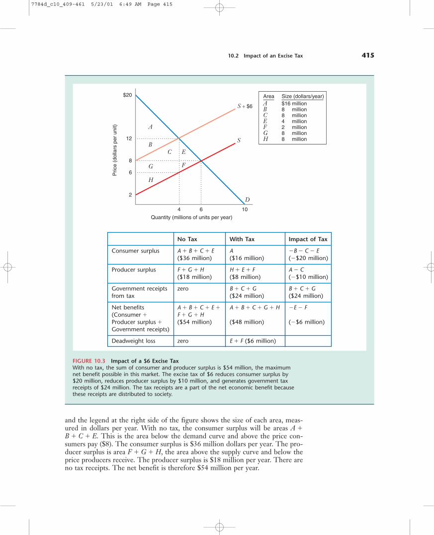
Now we can compare the equilibria with and without the excise tax.2 UsingFigure 10.3, we can calculate the consumer surplus, producer surplus and tax re-ceipts in the two cases. The areas of various portions of the graph are labeled,
Quantity (millions of units per year)
74 102 5 6
$20
12
10
4
98
2
6Pric
e (d
olla
rs p
er u
nit)
W
A
V
M
J S
S + $6
N
F
D
E
R
FIGURE 10.2 Equilibrium with an Excise TaxIf the government imposes an excise taxof $6 per unit, the total price collectedmust cover not only the price requiredby producers (on the supply curve), butalso the tax. The curve labeled “Supply�$6” shows what quantity producerswill offer for sale when the price chargedto consumers covers the marginal pro-duction cost plus the tax. The intersec-tion of the demand curve and the “Supply � 6” curve determines the equilibrium quantity, 4 million units.Consumers pay $12 per unit (at point Mon the graph), the government collectsthe $6 tax on each unit sold, and pro-ducers receive a price $6 (at point N.)
2The comparison of the market with and without the tax is an exercise in comparative statics, as de-scribed in Chapter 1. The exogenous variable is the size of the tax, which changes from zero to $6 perunit. We can ask how various endogenous variables (such as the quantity exchanged, the price producersreceive, and the price consumers pay) change as the size of the tax varies.
7784d_c10_409-461 5/23/01 6:49 AM Page 414
10.2 Impact of an Excise Tax 415
and the legend at the right side of the figure shows the size of each area, meas-ured in dollars per year. With no tax, the consumer surplus will be areas A �B � C � E. This is the area below the demand curve and above the price con-sumers pay ($8). The consumer surplus is $36 million dollars per year. The pro-ducer surplus is area F � G � H, the area above the supply curve and below theprice producers receive. The producer surplus is $18 million per year. There areno tax receipts. The net benefit is therefore $54 million per year.
Quantity (millions of units per year)
4 106
$20
12
8
2
6Pric
e (d
olla
rs p
er u
nit) A
B
G
H
S
C
F
E
S + $6
D
AreaABCEFGH
Size (dollars/year)$16 million8 million8 million4 million2 million8 million8 million
FIGURE 10.3 Impact of a $6 Excise TaxWith no tax, the sum of consumer and producer surplus is $54 million, the maximumnet benefit possible in this market. The excise tax of $6 reduces consumer surplus by$20 million, reduces producer surplus by $10 million, and generates government taxreceipts of $24 million. The tax receipts are a part of the net economic benefit becausethese receipts are distributed to society.
No Tax With Tax Impact of Tax
Consumer surplus A � B � C � E A �B � C � E($36 million) ($16 million) (�$20 million)
Producer surplus F � G � H H � E � F A � C($18 million) ($8 million) (�$10 million)
Government receipts zero B � C � G B � C � Gfrom tax ($24 million) ($24 million)
Net benefits A � B � C � E � A � B � C � G � H �E � F(Consumer � F � G � HProducer surplus � ($54 million) ($48 million) (�$6 million)Government receipts)
Deadweight loss zero E � F ($6 million)
7784d_c10_409-461 5/23/01 6:49 AM Page 415

416 CHAPTER 10 Competitive Markets: Applications
With the tax, the consumer surplus is $16 million, the size of area A. This isthe area under the demand curve and above the price consumers pay (Pd � $12).Producer surplus is $8 million, the size of area H. This is the area above the sup-ply curve and below the price producers receive (Ps � $6). As noted earlier, thetax receipts are a net benefit to society because they will be distributed over theeconomy. The tax receipts will be $24 million per year, the size of the rectangleB � C � G, reflecting the collection of the tax of $6 on each unit sold (the heightof the rectangle) times the 4 million units produced (the length of the rectangle).Thus, with the tax the annual net benefit is $48 million per year.
Finally, consider the row of the table labeled Net Benefits. It shows that theannual net benefit with the tax ($48 million) is smaller than the net benefit with-out the tax ($54 million). This loss in net benefits ($6 million per year) is calledthe deadweight loss resulting from the tax. The deadweight loss represents po-tential net economic benefits that no one (producers, consumers or the govern-ment) captures when the tax is imposed.
We can also understand how the deadweight loss arises by examining the rightcolumn in the table. It shows that the tax reduces consumer surplus by $20 mil-lion, reduces producer surplus by $10 million, and generates government tax re-ceipts of $24 million. When we add these changes (�$20 million � $10 million� $24 million), we find that net benefits decrease by $6 million, the size of thedeadweight loss.
The deadweight loss is the area E � F in Figure 10.3. This area is part of thenet benefit when there is no tax. E was a part of the consumer surplus with notax. The benefits in E disappeared because consumers reduced their purchasesfrom 6 to 4 million units with the tax. Similarly, F was a part of the producer sur-plus. But producers only supply 4 million units with the tax, and they thereforeno longer receive F.
E
S
D
LEARNING-BY-DOING EXERCISE 10.1
Excise Tax
In this exercise we reproduce the results illustrated in Figure 10.3, using alge-bra. The exercise will reinforce your understanding of how an excise tax worksin a competitive market.The demand and supply curves in the Figure 10.3 are as follows:
Qd � 10 � 0.5P d,
�2 � Ps, when Ps � 2,Qs � �0, when P s � 2
where Qd is the quantity demanded when the price consumers pay is Pd, andQs is the quantity supplied when the price producers receive is Ps. The last linesimply indicates that nothing will be supplied if the price producers receive isless than $2 per unit. Thus, for prices between zero and $2, the supply curvelies on the vertical axis.
7784d_c10_409-461 5/23/01 6:49 AM Page 416

10.2 Impact of an Excise Tax 417
Problem
(a) With no tax, what are the equilibrium price and quantity?(b) At the equilibrium in part (a), what is consumer surplus? Producer surplus?Deadweight loss? Show all of these graphically.(c) Suppose the government imposes an excise tax of $6 per unit. What willthe new equilibrium quantity be? What price will the buyer pay? What pricewill the seller receive?(d) At the equilibrium with the tax in part (c), what is consumer surplus? Pro-ducer surplus? The impact on the government budget (here a positive num-ber, the government tax receipts)? Deadweight loss? Show all of these graph-ically.(e) Verify for your answers to parts (b) and (d) that the following sum is identical:
Consumer surplus � Producer surplus � Tax receipts � Deadweight loss
Explain why the sum must be equal in both parts.
Solution With no tax, two conditions must be satisfied:(i) Pd � P s (there is no tax wedge). Since there is only one price in the mar-
ket, let’s call it P*.(ii) Also, the market clears, so that Qd � Qs.Together these conditions require that 10 � 0.5P* � �2 � P*, so the equi-
librium price, P* � $8 per unit. The equilibrium quantity can be found by sub-stituting P � $8 into either the supply or demand equation. If we use the de-mand equation, we find that the equilibrium quantity is Qd � 10 � 0.5(8) � 6million units.
The consumer surplus is the triangle A � B � C � E in Figure 10.3. Thearea of this triangle is 1/2[$(20 � 8) (6 million)], or $36 million. The producersurplus is the triangle G � H � F. The area of this triangle is 1/2[$(8 � 2) (6million)], or $18 million. There is zero deadweight loss at the competitive equi-librium.
With a $6 excise tax, there are two conditions that must be satisfied:(i) Pd � Ps � 6 (there is a tax wedge of $6).(ii) Also, the market clears, so that Qd � Qs, or 10 � 0.5Pd � �2 � Ps.Thus 10 � 0.5(Ps � 6) � �2 � Ps. The price producers receive is Ps � $6
per unit. The price consumers pay is Pd � Ps � $6 � $12. The equilibriumquantity can be found by substituting Pd � $12 into the demand equation, thatis Qd � 10 � 0.5Pd � 10 � 0.5(12) � 4 million units. (Alternatively, we couldhave substituted P s � $6 into the supply equation.)
The consumer surplus is area A in Figure 10.3. This area of this triangleis 1/2 [$(20 � 12) (4 million)] � $16 million. The producer surplus is areaH. This area of this triangle is 1/2[$(6 � 2) (4 million)] � $8 million. Thegovernment collects $6 on each of the 4 million units sold. The tax receiptsare thus $24 million per year (area B � C � G ). The size of the deadweightloss is the area of triangle (E � F ), or 1/2[$(12 � 6) (6 � 4) million] � $6million.
7784d_c10_409-461 5/23/01 6:49 AM Page 417

418 CHAPTER 10 Competitive Markets: Applications
INCIDENCE OF A TAX
In a market with an upward-sloping supply curve and a downward-sloping de-mand curve, an excise tax will cause the price consumers pay to rise, and the priceproducers receive to fall. Which price change will change more as a result of thetax? In Learning-By-Doing Exercise 10.1 the price the consumers pay increasesby $4 (rising from $8 to $12). The price the producers receive falls by $2 (de-creasing from $8 to $6). The incidence of the tax is the effect that the tax hason the prices consumers pay and sellers receive in a market. The incidence, orburden of the tax, is shared by both consumers and producers, although the largershare is borne by the consumers.
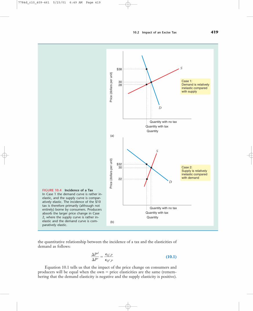
The incidence of the tax will depend on the shapes of the supply and demandcurves. Figure 10.4 illustrates two cases. In both cases the equilibrium price withno tax is $30 per unit. However, the effects of a tax of $10 are quite different inthe two markets.
In Case 1 the demand curve is relatively inelastic, and the supply curve isquite elastic. The tax causes consumers to pay $8 more than they would with notax. The tax also reduces the amount producers receive by $2. The price changeresulting from the tax is larger for consumers because the demand is compara-tively inelastic.
In Case 2 the tax has a larger impact on producers because the supply curveis relatively inelastic, while the demand curve is comparatively elastic. The taxdecreases the price producers receive by $8, while it increases the price consumerspay by only $2.
As the two cases suggest, the tax will have a larger impact on consumers ifthe demand is less elastic than the supply curve at the competitive equilibrium,and a larger impact on producers if the reverse is true. At least for small pricechanges, it is not unreasonable to assume that the demand and supply curves haveapproximately constant own-price elasticities, �Qd,P and �Qs,P. We can summarize
With no tax:
Consumer surplus ($36 million) � Producer surplus ($18 million) �Tax receipts (zero) � Deadweight loss (zero) � $54 million
With a $6 tax:
Consumer surplus ($16 million) � Producer surplus ($8 million) � Tax receipts ($24 million) � Deadweight loss
($6 million) � $54 million
Part (e) shows that the potential net benefit in the market is always $54 mil-lion. Consumers and producers capture all of the potential net benefits whenthere is no tax; there is no deadweight loss. With the tax, only $48 million ofthe potential net benefits are captured, so $6 million in potential benefits havedisappeared, becoming a deadweight loss. When the deadweight loss grows by adollar, the net benefits going to the economy must shrink by that dollar.
Similar Problem: 10.4, 10.6, 10.7
7784d_c10_409-461 5/23/01 6:49 AM Page 418
10.2 Impact of an Excise Tax 419
the quantitative relationship between the incidence of a tax and the elasticities ofdemand as follows:
PP
d
s � �
�
Q
Q
d
s,
,
P
P (10.1)
Equation 10.1 tells us that the impact of the price change on consumers andproducers will be equal when the own � price elasticities are the same (remem-bering that the demand elasticity is negative and the supply elasticity is positive).
Quantity with tax
Quantity
(a)
Quantity with no tax
$38
3028
Pric
e (d
olla
rs p
er u
nit)
S
D
Case 1:Demand is relativelyinelastic comparedwith supply
Quantity with tax
Quantity
(b)
Quantity with no tax
$3230
22
Pric
e (d
olla
rs p
er u
nit)
S
D
Case 2:Supply is relativelyinelastic comparedwith demand
FIGURE 10.4 Incidence of a TaxIn Case 1 the demand curve is rather in-elastic, and the supply curve is compar-atively elastic. The incidence of the $10tax is therefore primarily (although notentirely) borne by consumers. Producersabsorb the larger price change in Case2, where the supply curve is rather in-elastic and the demand curve is com-paratively elastic.
7784d_c10_409-461 5/23/01 6:49 AM Page 419

420 CHAPTER 10 Competitive Markets: Applications
EXAMPLE 10.1 Gasoline Taxes
In the late 1990s about 110 billion gallons of gasoline were purchased annually inthe United States. Although consumer prices fluctuate a great deal over time andvary by region, the price consumers paid at the pump (Pd) was about $1.10 pergallon at that time. Taxes on gasoline are often imposed not only at the federallevel, but also by state and local governments. Thus, the taxes paid vary by region.In most areas of the country, the total tax on gas was about $0.30 to $0.40 pergallon, although in some areas taxes were close to $0.50 per gallon.
In a “back of the envelope” exercise, let’s assume that the tax on gasoline (T)was $0.30 per gallon. This means that the price producers received (Ps) was about$0.80 per gallon. In the intermediate run of say, two to five years, it is reasonableto assume that the own-price elasticities of demand and supply are about�Qd,P � �0.5 and �Q s,P � �0.4.
Using the information about the current equilibrium, let’s examine two questions.
1. What quantities and prices would we anticipate if the taxes were removed?
2. Discussions of gasoline taxes sometimes suggest that for every increase ofone cent in the gasoline tax, the tax revenues collected will increase byabout $1 billion per year. Is this reasonable, at least for levels of taxes nearthe current $0.30 per gallon?
In this exercise we assume that the demand and supply curves are both lin-ear, and that the elasticities are correct at the equilibrium with the excise tax of
3To see why equation (10.1) is true, consider the effect of a small tax in a market. Suppose that the equilibrium price and quantity in the market with no tax are respectively P* and Q*. For a small tax, �Qd,P � Q/Q*/Pd/P*, which can be written as Q/Q* � Pd/P*�Qd,P. Similarly,�Qs,P � Q/Q*/Ps/P*, which means that Q/Q* � Ps/P*�Qs,P. Because the market will clear, a tax will reduce the quantity demanded and supplied by the same amount (Q/Q*). This requires that Pd/P* �Qd,P � Ps/P* �Qs,P, which can be simplified to equation (10.1).
For example, if �Qd,P � �0.5 and �Qs,P � �0.5, then Pd/Ps � �1. In otherwords, if a tax on $1 is imposed, the price consumers pay would rise by $0.50,while the price producers would receive would fall by $0.50.
As another example, suppose the supply is relatively elastic compared withdemand (for example, �Qd,P � �0.5 and �Qs,P � 2.0). Then Pd/P s � 2.0/�0.5 ��4. In this case the increase in the price consumers pay will be four times asmuch as the decrease in the price producers receive. Thus, if an excise tax of $1is imposed, the price consumers pay would rise by $0.80, while the price pro-ducers receive would fall by $0.20. The impact of the tax is therefore primarilyborne by consumers.3
Equation (10.1) explains much about the impact of federal and state taxes onmany markets. For example, the demands for goods such as alcohol and tobaccoare quite inelastic, while their supply curves are comparatively elastic. Thus, thegreater incidence of an excise tax falls on consumers in these markets.
7784d_c10_409-461 5/23/01 6:49 AM Page 420

10.2 Impact of an Excise Tax 421
$0.30 per gallon. Let’s begin by determining the equation of the demand curve,which must pass through point R in Figure 10.5, where the price is $1.10 and thequantity (measured in billions of gallons) is 110. If the demand curve is linear, ithas the form
Qd � a � bPd. (10.2)
Using the data, let us find the constants a and b in equation (10.2). By defini-tion, the own-price elasticity of demand is ��Qd,P � (Q/P)(Pd/Qd). In the lineardemand curve Q/P � �b. Thus, �0.5 � �b 1.10/110, which implies that b �50. Now we know that Qd � a � 50Pd. We can calculate a by using the price andquantity data at point R. Thus, 110 � a � 50(1.10), so a � 165. The equation ofthe demand curve is
Qd � 165 � 50Pd (10.3)
The equation of a linear supply curve (where e and f are constants) is
Qs � e � f Ps (10.4)
The own-price elasticity of supply is �Qs,P � (Q/P)(Ps/Qs). In equation (10.4),Q/P � f. Thus, at point W in Figure 10.5, 0.4 � f 0.8/110, or f � 55. Therefore,Qs � e � 50Ps. We can calculate e by using the price and quantity data at point W.
Quantity (billions of gallons of gasoline per year)
117.9
Tax of $0.30per gallon
110
$1.10
0.94
0.80
Pric
e (d
olla
rs p
er g
allo
n) S
R
W
E
D
FIGURE 10.5 Effects of Gasoline TaxWith an excise tax of $0.30 per gallon, consumers pay about $1.10 per gallon (atpoint R), and producers receive about $0.80 per gallon (at point W ). If there were notax, the equilibrium price would be about $0.94 per gallon (at point E). The incidenceof the tax is shared nearly equally by consumers and producers.
7784d_c10_409-461 5/23/01 6:49 AM Page 421
422 CHAPTER 10 Competitive Markets: Applications
Thus, 110 � e � 55(0.8), which means that e � 66. So the equation of the demandcurve is
Qs � 66 � 55Ps. (10.5)
The supply and demand curves are drawn in Figure 10.5. If there were no taxes,the equilibrium price P* would be at point E, where P* � Ps � Pd (there is no taxwedge). Using the market clearing condition (Qs � Qd), we find that 165 � 50P* �66 � 55P*. The equilibrium price is P* � $0.94 per gallon. With no tax, about 118billion gallons of gas would be sold.
Note that the incidence of the current tax (T � $0.30 per gallon) is rather evenlyshared by consumers and producers. This is not surprising because the elasticitiesof supply and demand are about the same. With the tax consumers pay $1.10 in-stead of $0.94 per gallon. Similarly, producers receive $0.80 with the tax insteadof $0.94 without it.
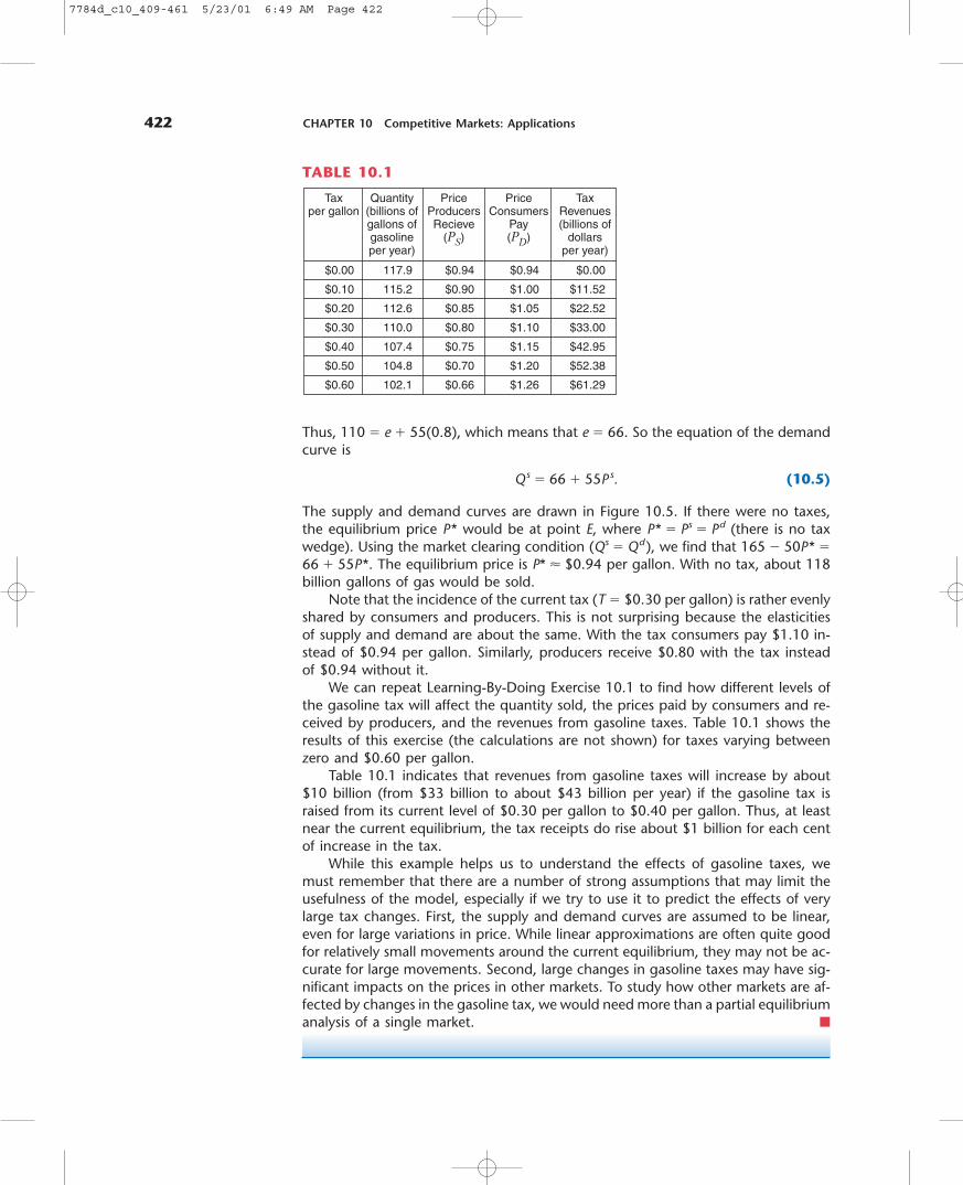
We can repeat Learning-By-Doing Exercise 10.1 to find how different levels ofthe gasoline tax will affect the quantity sold, the prices paid by consumers and re-ceived by producers, and the revenues from gasoline taxes. Table 10.1 shows theresults of this exercise (the calculations are not shown) for taxes varying betweenzero and $0.60 per gallon.
Table 10.1 indicates that revenues from gasoline taxes will increase by about$10 billion (from $33 billion to about $43 billion per year) if the gasoline tax israised from its current level of $0.30 per gallon to $0.40 per gallon. Thus, at leastnear the current equilibrium, the tax receipts do rise about $1 billion for each centof increase in the tax.
While this example helps us to understand the effects of gasoline taxes, wemust remember that there are a number of strong assumptions that may limit theusefulness of the model, especially if we try to use it to predict the effects of verylarge tax changes. First, the supply and demand curves are assumed to be linear,even for large variations in price. While linear approximations are often quite goodfor relatively small movements around the current equilibrium, they may not be ac-curate for large movements. Second, large changes in gasoline taxes may have sig-nificant impacts on the prices in other markets. To study how other markets are af-fected by changes in the gasoline tax, we would need more than a partial equilibriumanalysis of a single market. �
Taxper gallon
Quantity(billions ofgallons ofgasolineper year)
PriceProducersRecieve
(PS)
PriceConsumers
Pay(PD)
TaxRevenues(billions of
dollarsper year)
$0.00 117.9 $0.94 $0.94 $0.00
$0.10 115.2 $0.90 $1.00 $11.52
$0.20 112.6 $0.85 $1.05 $22.52
$0.30 110.0 $0.80 $1.10 $33.00
$0.40 107.4 $0.75 $1.15 $42.95
$0.50 104.8 $0.70 $1.20 $52.38
$0.60 102.1 $0.66 $1.26 $61.29
TABLE 10.1
7784d_c10_409-461 5/23/01 6:49 AM Page 422

10.3 Subsidies 423
Instead of taxing a market, a government might decide to subsidize it. We canthink of a subsidy as a negative tax. With a subsidy of T per unit, the price pro-ducers receive (Ps) will be the price consumers pay (Pd ) plus the subsidy T. Asyou might suspect, the effects of a subsidy are opposite those of a tax.
• The market will overproduce relative to the efficient level.• Consumer surplus will be higher than with no subsidy.• Producer surplus will be higher than with no subsidy.• The impact on the government budget will be negative. Government expendi-
tures on the subsidy are a negative net benefit since the money to pay for thesubsidy must be collected elsewhere in the economy.
• Government expenditures on the subsidy will be larger than the increase inconsumer and producer surplus. Thus, there will be a deadweight loss fromoverproduction.
In Figure 10.6 shows how a subsidy of $3 per unit affects the competitivemarket with the supply and demand curves in Learning-By-Doing Example 10.1.The figure shows a new curve (labeled Supply � 3) which subtracts the amountof the subsidy vertically from the supply curve. This curve tells us how much pro-ducers will offer for sale when the price received by producers includes the priceconsumers pay plus the subsidy.
We can find the equilibrium with the subsidy by looking at the intersec-tion of the demand curve and the Supply � 3 curve. In Figure 10.6 the market-clearing quantity is Q1 � 7 million units per year. Producers receive a price Ps �$9 per unit, including the price consumers pay Pd � $6, and the subsidy the gov-ernment pays $3 per unit.
We can compare the equilibria with and without the subsidy. From Exercise10.1 we know that the consumer surplus with no subsidy is $36 million per year.Using the labels in Figure 10.6, the consumer surplus is areas A � B. The pro-ducer surplus is $18 million per year (E � F ). There are no government expen-ditures. The net benefit is therefore $54 million (A � B � E � F).
With the subsidy the consumer surplus is $49 million, the area A � B � E �G � K, below the demand curve and above the $6 price consumers pay. Annualproducer surplus is $24.5 million, the area B � C � E � F, above the supply curveand below the $9 price producers receive. The subsidy costs the government $21million per year, the area of rectangle B � C � E � G � K � J, reflecting thesubsidy of $3 on each unit produced (the height of the rectangle) times the 7 mil-lion units produced per year (the length of the rectangle). The expenditures areshown as a negative benefit in the table because they must be financed by taxescollected elsewhere in the economy.
Finally, consider the row of the table labeled “Net Benefits.” It shows thatthe annual net benefit with the subsidy is $52.5 million, smaller than the net ben-efit without the subsidy by area J, which measures $1.5 million. This is the dead-weight loss resulting from the subsidy.
We can also find the deadweight loss by examining the right column in the table.It shows that the subsidy increases consumer surplus by $13 million (E � G � K ),increases producer surplus by $6.5 million (B � C), and costs the government $21million (�B � C � E � G � K � J ). As before, when we add these changes, we findthat net benefits decrease by $1.5 million, the deadweight loss represented by area
10.3SUBSIDIES
7784d_c10_409-461 5/23/01 6:49 AM Page 423

424 CHAPTER 10 Competitive Markets: Applications
J. The deadweight loss arises because the quantity produced rises from 6 millionunits with no subsidy, to 7 million with the subsidy. Over that range of output thesupply curve lies above the demand curve, so net benefits are reduced as each ofthese units is produced. Thus, net economic benefits are reduced because the sub-sidy causes market to overproduce relative to the efficient level.
Quantity (millions of units per year)
Q1 = 7 10Q* = 6
$20
2
PS = 9P* = 8
PD = 6Pric
e (d
olla
rs p
er u
nit)
A
B
G KJ
S
C
F
E
D
S
S − $3
Subsidy of $3per unitproduced
FIGURE 10.6 Subsidy on Each Unit ProducedWith a subsidy of $3 per unit, the price producers receive (PS � $9) is the price consumerspay (PD � $6) plus the subsidy of $3. The market clears at 7 million units, above the effi-cient level of 6 million units. For each unit produced between Q* and Q1, the supplycurve lies above the demand curve, indicating that the marginal cost exceeds the valueconsumers place on those units. The deadweight loss J occurs because of the overproduc-tion relative to the efficient level Q*.
No Subsidy With Subsidy Impact of Subsidy
Consumer surplus A � B A � B � E � G � K E � G � K($36 million) ($49 million) ($13 million)
Producer surplus E � F B � C � E � F B � C($18 million) ($24.5 million) ($6.5 million)
Impact on government zero � B � C � E � G � K � J � B � C � E � G � K � Jbudget (�$21 million) (�$21 million)
Net benefits A � B � E � F A � B � E � F � J �J(Consumer � ($54 million) ($52.5 million) (�$1.5 million)Producer surplus �Government receipts)
Deadweight loss zero J ($1.5 million)
7784d_c10_409-461 5/23/01 6:49 AM Page 424

10.4 Price Ceilings (Maximum Price Regulation) 425
E
S
D
LEARNING-BY-DOING EXERCISE 10.2
Subsidy
Problem
(a) Using the supply and demand curves in Learning-By-Doing Example 10.1,use algebra to find the equilibrium for a subsidy of $3 per unit. Find the equi-librium quantity, the price the buyers pay, and the price the sellers receive.(b) In Learning-By-Doing Exercise 10.1, we found that the potential net ben-efits in the market are Consumer surplus � Producer surplus � Tax receipts �Deadweight loss � $54 million. For the case of the subsidy, show that the po-tential net benefits (Consumer surplus � Producer surplus � Subsidy (a neg-ative number) � Deadweight loss) are still $54 million.
Solution With a $3 subsidy, two conditions must be satisfied in equilibrium:(i) Pd � Ps � 3 (there is a subsidy wedge of $3).(ii) Also, the market clears, so that Qd � Qs, or 10 � 0.5Pd � �2 � Ps.These conditions require that 10 � 0.5(Ps � 3) � �2 � Ps, which means
that producers receive a price of $9 (Ps � $9) in equilibrium. The equilibriumprice consumers pay is Pd � Ps � $3 � $6 per unit. The equilibrium quantitycan be found by substituting Pd � $6 into the demand equation, that is Qd �10 � 0.5Pd � 10 � 0.5(6) � 7 million units. (Alternatively, we could have sub-stituted Ps � $9 into the supply equation.)
With the $3 subsidy:
Consumer surplus ($49 million) � Producer surplus ($24.5 million) �Expenditures on subsidy (�$21 million) � Deadweight loss ($1.5 million) �
$54 million
Part (b) is similar to part (e) of Learning-By-Doing Exercise 10.1. It remindsus that the potential net benefits are the same, whether the market is efficientor not. With no subsidy we know there is no deadweight loss and the net ben-efit is $54 million. With the subsidy, the net benefits to society are $52.5 mil-lion, so $1.5 million in potential benefits have disappeared. Again, the impor-tant point is that if the deadweight loss grows by a dollar, the net benefits goingto the economy must shrink by that dollar.
Similar Problem: 10.6
Sometimes a government may set a maximum allowable price in a market, suchas the price of food, gasoline, crude oil, or the rental price for housing. If theprice ceiling is below the price in a market with an upward-sloping supply curveand a downward-sloping demand curve, the ceiling has the following effects:
• The market will not clear. There will be an excess demand for the good.
10.4PRICECEILINGS(MAXIMUMPRICEREGULATION)
7784d_c10_409-461 5/23/01 6:49 AM Page 425

426 CHAPTER 10 Competitive Markets: Applications
• The market will underproduce relative to the efficient level (that is, the amountthat would be supplied in an unregulated market).
• Producer surplus will be lower than with no price ceiling.• Some (but not all) of the lost producer surplus will be transferred to con-
sumers.• Because there is excess demand with a price ceiling, the size of the consumer
surplus depends on which of the consumers who want the good are able to pur-chase it. Consumer surplus may either increase or decrease with a price ceiling.
Let’s examine the effects of a price ceiling with rent controls. For decadesrent controls have been in force in many cities around the world. Rent controlsare legally imposed ceilings on the rents that landlords may charge their tenants.They often originated as temporary ceilings imposed in the inflationary time ofwar, as was the case in London and Paris during World War I, in New York dur-ing World War II, and in Boston and several nearby suburbs during the Vietnamconflict in the late 1960s and early 1970s.
In 1971 President Nixon imposed wage and price controls throughout theUnited States, freezing all rents. After the federal controls expired, many city gov-ernments continued to place ceilings on rents. In 1997 William Tucker noted,“During the 1970s it appeared that rent control might be the wave of the future...By the mid-1980s, more than 200 separate municipalities nationwide, encom-passing about 20 percent of the nation’s population, were living under rent con-trol. However, this proved to be the high tide of the movement. As inflationarypressures eased, the agitation for rent control subsided.”4
Figure 10.7 illustrates the supply and demand curves in the market for a par-ticular type of housing, such as the market for studio apartments in New YorkCity. For various rental prices the supply curve shows how many units landlordswould be willing to make available, and the demand curve indicates how manyunits consumers would like to rent. If there were no rent controls, the market forstudio apartments would clear at a rental price of $1600 per month and 80,000units being rented.
If there is no rent control, the market clears. Every consumer who is willingto pay the equilibrium price of $1,600 (consumers between points Y and V onthe demand curve) will find housing. Further, every landlord willing to supplyhousing at that price (those at between point Z and V on the supply curve) willserve the market. Consumer surplus will be area A � B � E, and producer sur-plus will be area C � F � G. The sum of consumer and producer surplus willtherefore be A � B � C � G � E � F.
Suppose the government imposes rent control by setting a maximum rental priceof $1,000 per month. At that price landlords will be willing to supply 50,000 units(point W on the supply curve). The rent control has moved landlords from point Vto point W on the supply curve, reducing the supply of housing by 30,000 units.
When a price ceiling is set below the unregulated market price, the marketdoes not clear. When the price ceiling is $1,000, consumers would like to rent 140,000 units (point X on the demand curve). But, as we have already noted,landlords offer only 50,000 units for rent. There is therefore an excess demand
4William Tucker, “How Rent Control Drives Out Affordable Housing,” Cato Policy Analysis, paper no.274 (Washington, D.C.: The Cato Institute, May 21, 1997).
7784d_c10_409-461 5/23/01 6:49 AM Page 426
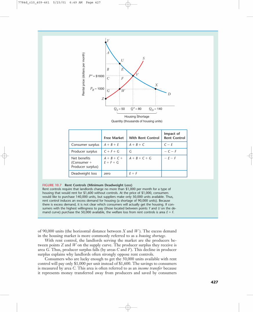
of 90,000 units (the horizontal distance between X and W ). The excess demandin the housing market is more commonly referred to as a housing shortage.
With rent control, the landlords serving the market are the producers be-tween points Z and W on the supply curve. The producer surplus they receive isarea G. Thus, producer surplus falls (by areas C and F ). This decline in producersurplus explains why landlords often strongly oppose rent controls.
Consumers who are lucky enough to get the 50,000 units available with rentcontrol will pay only $1,000 per unit instead of $1,600. The savings to consumersis measured by area C. This area is often referred to as an income transfer becauseit represents money transferred away from producers and saved by consumers
Q* = 80 QD = 140QS = 50
Z
P* = $1600
PR = 1000
Ren
tal p
rice
(dol
lars
per
mon
th)
Y
A
B
C
G
E
U
V
X
D
S
F
W
Housing Shortage
Quantity (thousands of housing units)
FIGURE 10.7 Rent Controls (Minimum Deadweight Loss)Rent controls require that landlords charge no more than $1,000 per month for a type ofhousing that would rent for $1,600 without controls. At the price of $1,000, consumerswould like to purchase 140,000 units, but suppliers make only 50,000 units available. Thus,rent control induces an excess demand for housing (a shortage of 90,000 units). Becausethere is excess demand, it is not clear which consumers will actually get the housing. If con-sumers with the highest willingness to pay (those located between points Y and U on the de-mand curve) purchase the 50,000 available, the welfare loss from rent controls is area E � F.
Impact of Free Market With Rent Control Rent Control
Consumer surplus A � B � E A � B � C C � E
Producer surplus C � F � G G � C � F
Net benefits A � B � C � A � B � C � G � E � F(Consumer � E � F � GProducer surplus)
Deadweight loss zero E � F
427
7784d_c10_409-461 5/23/01 6:49 AM Page 427
428 CHAPTER 10 Competitive Markets: Applications
who are lucky enough to get the housing available under rent controls. Observethat area F is part of the lost producer surplus, but not part of the income trans-fer. The units of housing between W and V on the supply curve are not producedat all under rent control. The potential benefits in area F disappear with rent con-trol, becoming part of the deadweight loss.
How will consumer surplus be affected by rent controls? To answer this ques-tion, we must recognize that all of the consumers between Y and X on the de-mand curve want housing at a price of $1,000, but only some of them will findit. Since only 50,000 units are available, we need to know which of the 140,000consumers who want the housing at $1,000 will be able to find housing. Let’sconsider two possible answers to this question.
• Case 1. Consumers with the highest willingness to pay receive the housing. One pos-sibility is that the consumers with the highest willingness to pay receive thehousing. Here consumers between Y and U on the demand curve would be theones lucky enough to find housing. The other consumers between U and Xwould be unable to do so, even though they are willing to pay $1,000. Withthis allocation of housing, the consumer surplus is area A � B � C (the areabelow the demand curve and above the rental price of $1,000). This is themaximum possible consumer surplus with rent control. As Figure 10.7 indi-cates, the sum of consumer and producer surplus is A � B � C � G. The rentcontrol creates a deadweight loss of E � F, the amount of the reduction in thesum of consumer and producer surplus. The deadweight loss arises because theamount of housing available in the market has been reduced from 80,000 unitsin the unregulated market to 50,000 with rent control. With rent control thepotential net benefits represented by the area E � F are lost to society.
• Case 2. Consumers with the lowest willingness to pay receive the housing. A second pos-sibility is that the 50,000 available units are rented by those consumers with thelowest willingness to pay. In Figure 10.8 these consumers are the ones between Tand X on the demand curve.5 The other consumers between Y and T are unableto find housing, even though they are willing to pay more than $1,000.
With this allocation of housing, the consumer surplus is area H (again, thearea below the demand curve and above the rental price of $1000). This is the minimum possible consumer surplus with rent control. As Figure 10.8 indi-cates, the sum of consumer and producer surplus is G � H. Rent control now cre-ates a deadweight loss of E � F � A � B � C � H. The deadweight loss is largerin Case 2 than in Case 1 because the consumer surplus is smaller in Case 2.
The two cases just considered define upper and lower limits on the consumersurplus and deadweight loss from rent controls. The producer surplus will be areaG in either case. The maximum consumer surplus and the minimum deadweightloss are shown in Case 1. The minimum consumer surplus and the maximumdeadweight loss are shown in Case 2. The actual consumer surplus and dead-weight loss may be in between the levels in these two polar cases. To find the exact consumer surplus and the deadweight loss, we would need to know moreabout how the available housing is allocated.
5We do not consider consumers to the right of point X on the demand curve because they would not bewilling to rent housing at $1,000 even if they could find it.
7784d_c10_409-461 5/23/01 6:49 AM Page 428

10.4 Price Ceilings (Maximum Price Regulation) 429
Most textbooks depict the effects of a price ceiling with a graph like the onein Figure 10.1, assuming that the good ends up in the hands of consumers withthe highest willingness to pay. This assumption is reasonable when consumerscan easily resell the good to other consumers with a higher willingness to pay.The following example illustrates how resale enables consumers toward the upper end of the demand curve to buy the good in a resale market, even thoughthey might not be able to obtain the good when it is initially sold.
9080 QD = 140QS = 50
Z
P* = $1,600
PR = 1,000
Ren
tal p
rice
(dol
lars
per
mon
th)
Y
A
B
C
G
E
U
VT
H X
D
S
F
W
Housing Shortage
Quantity (thousands of housing units)
FIGURE 10.8 Rent Controls (Maximum Deadweight Loss)The market does not clear with rent controls. Because there is excess demand, it is notclear which consumers will actually get the housing. If consumers with the lowest willing-ness to pay (those located between points T and X on the demand curve) purchase the50,000 units available, the consumer surplus with rent control will be area H. Producersurplus with rent control is still area G, as in Figure 10.7. The welfare loss from rent con-trols will be much larger than in Figure 10.7 because consumer surplus is lower whenconsumers with the lowest willingness to pay rent the housing.
Impact of Free Market With Rent Control Rent Control
Consumer surplus A � B � E H H � A � B � E
Producer surplus C � F � G G � C � F
Net benefits A � B � C � G � H � E � F � A � B � C � H(Consumer � E � F � GProducer surplus)
Deadweight loss zero E � F � A � B � C � H
7784d_c10_409-461 5/23/01 6:49 AM Page 429

430 CHAPTER 10 Competitive Markets: Applications
EXAMPLE 10.2 Scalping Super Bowl Tickets on the Internet
When the National Football League (NFL) sells tickets to the Super Bowl, it es-tablishes face values (the prices printed on the tickets) that are far below the market prices. The NFL understands that there will be a large excess demand fortickets sold at face value. It therefore accepts requests for tickets a year in ad-vance of the event, and then chooses the recipients of the tickets in a randomdrawing.
Face prices for tickets to Super Bowl XXXIV in Atlanta in 2000 ranged from$325 to $400, depending on the location of the tickets. Because of the excess de-mand, there was an active resale market for tickets. In the month before the gameseveral sites on the Internet offered box seats at prices around $4,500, more thanten times the face value of the ticket.
The winners of the random drawing are indeed lucky. They can use the ticketsthemselves, or resell the tickets at a handsome profit. The existence of an easily ac-cessible, active resale market helps move the tickets ultimately into the hands ofpeople who most highly value the opportunity to see the game in person.
Beyond the face value of the ticket and the attractiveness of the event, twotypes of transactions costs affect the possibility of resale. First, in some states re-sale (“scalping”) is illegal. A law prohibiting resale is likely to be more effectivewhen the penalty for a violation is high and when the probability of being caughtreselling is high. Even though resale is illegal in many areas, it may neverthelessbe common where penalties are low or there is little risk of being caught. Second,resellers incur transactions costs in searching out supplies of tickets and locatingbuyers.
In recent years the Internet has lowered both types of transactions costs con-siderably. Buyers and sellers can conduct business from the comfort of home or theoffice. With a Web site, scalpers can widely advertise tickets at a very low cost andwith less risk of being caught than would be the case if the transactions took placein the shadow of the stadium.
If resale involves low transactions costs, total surplus will be close to the max-imum possible, as assumed in Case 1 (Figure 10.7) in the discussion of price ceil-ings. Part of the surplus may go to middlemen (scalpers and brokers) instead ofthe final holders of the tickets, but the net benefits do not disappear from theeconomy.
Of course, scalping typically involves a certain amount of risk, including thepossibility that the tickets are not as desirable as advertised, or perhaps are not validat all. Those supporting laws against scalping often cite examples of fraud. If theoriginal sellers of tickets or governing authorities are willing to impose very strictconditions, it may be possible to reduce resale greatly. For example, the seller couldput the buyer’s picture on the ticket (as is often done with monthly passes on ur-ban transport systems), or write the buyer’s name on the ticket and require thebuyer to produce a picture I.D. when she uses the ticket (as the airlines often do).However, these measures add significant costs to businesses and to law enforce-ment efforts, and are often difficult to implement. �
7784d_c10_409-461 5/23/01 6:49 AM Page 430

10.4 Price Ceilings (Maximum Price Regulation) 431
Before leaving rent controls, we note that government attempts to regulatethe price of a commodity rarely work in a straightforward fashion. For example,when a shortage develops in the rental market for housing, some landlords maydemand key money,—that is, an extra payment from a prospective renter—be-fore agreeing to lease an apartment. Although such payments are illegal, theyare difficult to monitor, and renters who are willing to pay more than the rentcontrolled price may willingly (though not happily) pay the key money. Land-lords may also recognize that with excess demand, they will be able to find renterseven if they allow the quality of the apartments to deteriorate. Rent control lawsoften attempt to specify that the quality should be maintained, but it is quite dif-ficult to write the laws to enforce this intent effectively. Further, landlords mayrecognize that they would be better off in the long run if they can convert apart-ments under rent control to other uses not subject to price controls, such as con-dominiums or even parking lots. Critics of rent controls often observe that theamounts of housing available have been reduced over time as owners of con-trolled housing convert to alternative uses of land.6
We must remember that there are limitations in a partial equilibrium analy-sis of the effect of a price ceiling, such as the one in Figures 10.7 and 10.8. If a rent control is imposed in the market for studio apartments, people who can-not find a studio apartment will seek another type of housing, such as a largerapartment, a condominium, or even a house. This will affect the demand for other types of housing, and thus the equilibrium prices in those markets. As theprices of other types of housing change, the demand for studio apartments mayshift, resulting in additional consequences on the size of the shortage of studioapartments, as well as consumer and produce surplus and deadweight loss. Cal-culating these additional effects is beyond the scope of a simple partial equi-librium analysis, but you should recognize that they may be important.
The unintended consequences of price ceilings are present in many marketsother than housing. For example, in an effort to fight inflation in the 1970s theNixon administration imposed price ceilings on domestic suppliers of oil, creat-ing a shortage of domestic oil. The excess demand for oil led to increased im-ports of oil. When the price controls were imposed in 1971, imports constitutedonly 25 percent of the nation’s supply. As time passed, the shortage grew sub-stantially. By 1973, imports made up nearly 33 percent of the total oil consumedin the United States. OPEC countries recognized the growing dependence onimports in the United States, and they responded by quadrupling the price ofimported oil. In the end the domestic price controls contributed to still higherinflation in the United States, working against the intent of the original pricecontrols.7
6See, for example, Denton Marks, “The Effects of Partial-Coverage Rent Control on the Price andQuantity of Rental Housing,” Journal of Urban Economics, 16 (1984): 360–369.7See George Horwich and David Weimer, “Oil Price Shocks, Market Response, and Contingency Plan-ning,” The American Enterprise Institute, Washington, D.C., 1984.
7784d_c10_409-461 5/23/01 6:49 AM Page 431

432 CHAPTER 10 Competitive Markets: Applications
EXAMPLE 10.3 Price Ceilings in the Market for Natural Gas
Following a decision of the U.S. Supreme Court in 1954 (Phillips Petroleum Com-pany v. Wisconsin, et. al.), the federal government regulated the price of natural gassold in interstate commerce, that is, gas produced in one state (such as Texas) andsold to consumers or industries in another state (such as Ohio). By contrast, well-head prices in intrastate markets (for example, gas produced and sold in Texas)were not regulated.
For several years following this historic decision, the Federal Power Commissionimposed ceiling price regulations on natural gas at the wellhead, the point at whichnatural gas leaves the ground. Prior to 1962 the ceiling price was above the pricethat cleared the interstate market for natural gas. Thus, before 1962 the ceilingprice constraints were not binding, and the market cleared.
Figure 10.9(a) illustrates a market with price ceiling PR higher than the equi-librium price P*. At the equilibrium price all buyers and sellers were satisfied, andthe price ceiling was not violated. Thus, the price ceiling had no effect on the market.
After 1962 the ceiling price did become binding, and excess demand began todevelop in the industry. The shortage of natural gas became severe as the price ofoil rose in the world market and many consumers wanted to switch to natural gasfor heating. Absent a price ceiling, the market-clearing price of natural gas in theinterstate market would have been about $2 per MCF (thousand cubic feet) in themid-1970s.8 However, federal regulations imposed a price ceiling of about $1 perMCF, as Figure 10.9(b) illustrates. At the price ceiling the quantity of gas supplied(Qs) was about two-thirds of the quantity demanded (Qd), creating a severe short-age of natural gas in interstate markets.
The deadweight loss was at least the area bounded by the points UVW. Sinceresale of natural gas at higher prices was illegal, some consumers between U andX may have received gas, displacing consumers with higher willingnesses to pay.The deadweight loss was therefore probably greater than UVW.
The widespread shortages of natural gas caused national concern, especiallybecause many people in the Midwest and Northeast could not purchase naturalgas to heat their homes. In some states, such as Ohio, many schools were forcedto close because they were unable to find enough natural gas to heat schools. Theshortages, along with the difficulty of administering a complex set of price controlsfor thousands of producers, led to the deregulation of natural gas prices starting in1978. �
8Natural gas was selling for about $2 per MCF in unregulated intrastate markets, leading analysts to be-lieve that the equilibrium price in the interstate market would have also been about $2 if the price ceil-ing were removed.
7784d_c10_409-461 5/23/01 6:49 AM Page 432

10.4 Price Ceilings (Maximum Price Regulation) 433
QD QS
P*
Q*
PR
Pric
e (d
olla
rs p
er M
CF
)
S
D
Y
V
Quantity of gas (MCF)
QS QD
P* = $2 per MCF
Q*
PR = $1 per MCF
Pric
e (d
olla
rs p
er M
CF
)
S
D
Y
VX
W
U
Quantity of gas (MCF)
(a) Nonbinding price ceiling, before 1962
(b) Binding price ceiling, mid-1970s
Shortage of natural gas
FIGURE 10.9 Price Ceilings for Natural GasBefore 1962, the ceiling price on naturalgas sold in interstate markets (PR) washigher than the equilibrium price (P*).The ceiling had no effect on the marketsince the market cleared at a price be-low the ceiling.
By the mid-1970s, the maximum al-lowed price was lower than the equilib-rium price. The ceiling induced a severeshortage, with the quantity supplied be-ing only about two-thirds of the quan-tity demanded. The deadweight losswas at least the area bounded by thepoints UVW (assuming that the con-sumers between Y and U on the de-mand curve were the ones who re-ceived the gas). Resale in this marketwas illegal. Some consumers between Uand X may have received gas, displacingconsumers with higher willingnesses topay. The deadweight loss was probablygreater than UVW.
E
S
D
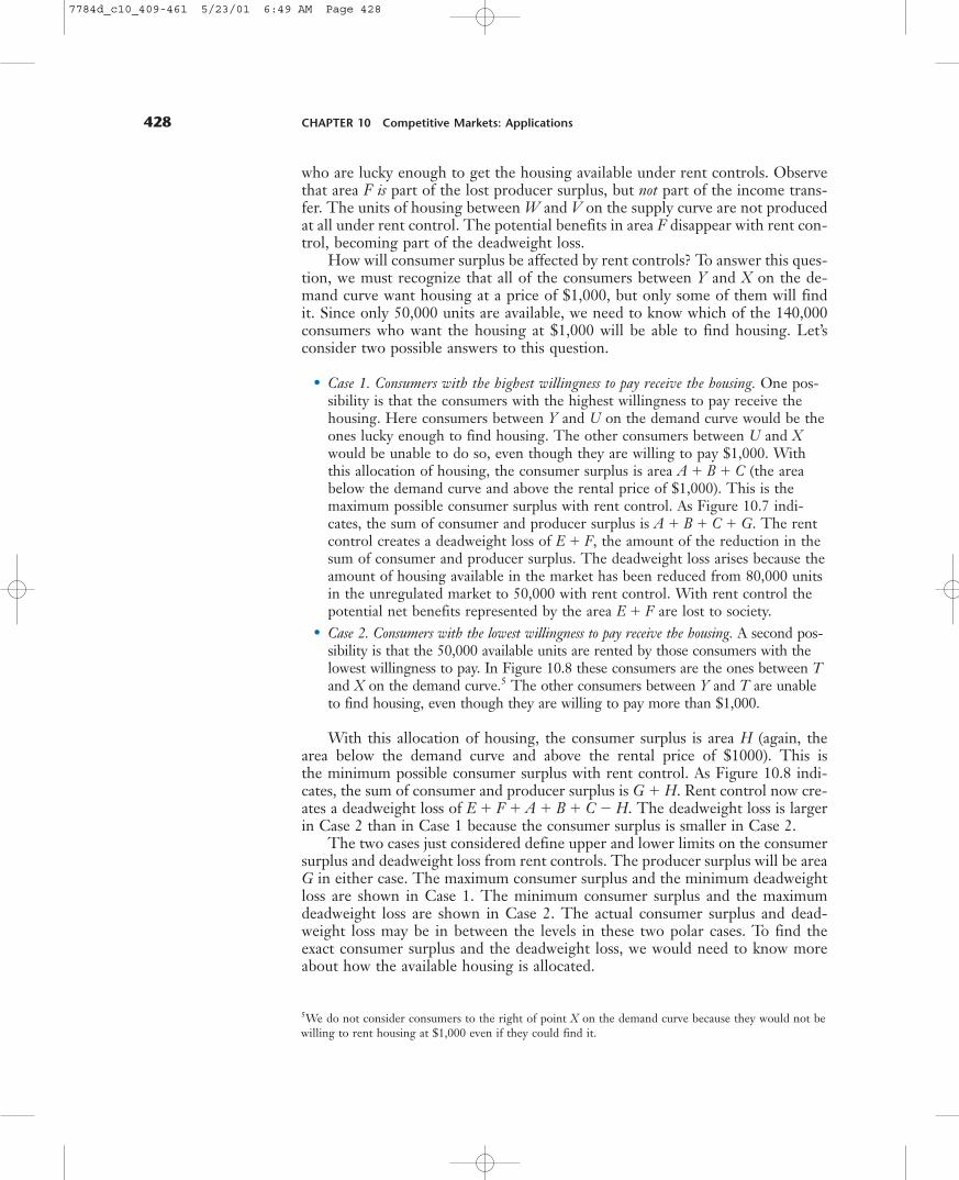
LEARNING-BY-DOING EXERCISE 10.3
Effect of a Price Ceiling
The supply and demand curves illustrated in Figure 10.10 are the same oneswe have used in the previous two Learning-By-Doing Exercises. Suppose thegovernment imposes a price ceiling of $6 in the market.
7784d_c10_409-461 5/23/01 6:49 AM Page 433
434 CHAPTER 10 Competitive Markets: Applications
Problem
(a) What is the size of the shortage in the market with the price ceiling? Whatis the producer surplus?(b) What is the maximum consumer surplus, assuming the good is purchasedby consumers with the highest willingness to pay? What is the deadweight loss?(c) What is the minimum consumer surplus, assuming the good is purchasedby consumers with the lowest willingness to pay? What is the deadweight loss?(d) With no price ceiling, the sum of consumer and producer surplus wouldbe area YVZ ($54 million). For your answers to parts (b) and (c), show that thepotential net benefits (Consumer surplus � Producer surplus � Deadweightloss) are $54 million.
Pric
e (d
olla
rs p
er u
nit)
Y
U
T
X
S
D
WR
Z
S
A V
Quantity (millions of units per year)
3 64 7 10
Priceceiling
2
6
8
12
14
$20
FIGURE 10.10 Price Ceiling: Learning-By-Doing Exercise 10.3With no regulation, the equilibrium price would be $8, and the sum of consumer andproducer surplus is the area YVZ ($54 million). With a price ceiling of $6, producerssupply 4 million units, and consumers demand 7 million units. There is an excess de-mand of 3 million units. Producer surplus is the area SWZ ($8 million). The size of theconsumer surplus depends on which consumers are able to purchase the good:
Case 1. Maximum Consumer Surplus: If consumers with the highest willingness to pay(those between Y and T on the demand curve) purchase the 4 million units supplied, con-sumer surplus will be the area YTWS ($40 million). The sum of consumer surplus ($40 mil-lion) and producer surplus ($8 million) is $48 million, or $6 million short of the total sur-plus possible in an unregulated market. This $6 million deadweight loss is area TWV.
Case 2. Minimum Consumer Surplus: If the consumers with the lowest willingnessto pay (those between U and X on the demand curve) purchase the 4 million unitssupplied, consumer surplus will be the area URX ($16 million). Now the sum of con-sumer surplus ($16 million) and producer surplus ($8 million) is only $24 million, or$30 million short of the total surplus possible in an unregulated market. The dead-weight loss in Case 2 is therefore $30 million.
7784d_c10_409-461 5/23/01 6:49 AM Page 434

10.5 Price Floors (Minimum Price Regulation) 435
Solution If the ceiling price is $6, consumers demand 7 million units, butproducers supply only 4 million. The excess demand (shortage) is 3 millionunits, the horizontal distance between W and X in the figure.
The producer surplus is the area of the triangle below the ceiling price of $6 and above the supply curve. Producer surplus will be the area SWZ ($8million).
Suppose consumers with the highest willingness to pay (those between Yand T on the demand curve) purchase the 4 million units available. Consumersurplus will be the area YTWS ($40 million). The sum of consumer surplus($40 million) and producer surplus ($8 million) is $48 million.
How much is the deadweight loss? With the price ceiling the consumer andproducer surplus is only $48 million, or $6 million short of the total surpluspossible in an unregulated market. This $6 million deadweight loss is areaTWV.
If consumers with the lowest willingness to pay (those between U and X onthe demand curve) purchase the 4 million units available, consumer surpluswill be the area URX ($16 million). The sum of consumer surplus ($16 mil-lion) and producer surplus ($8 million) is only $24 million, or $30 million shortof the total surplus possible in an unregulated market ($54 million). The dead-weight loss in Case 2 is ($30 million).
For part (b): Consumer surplus ($40 million) � Producer surplus ($8 mil-lion) � Deadweight loss ($6 million) � $54 million
For part (c): Consumer surplus ($16 million) � Producer surplus ($8 million) � Deadweight loss ($30 million) � $54 million
Once again, this exercise shows the potential surplus is the same with orwithout intervention. Every dollar of the potential surplus that is not capturedbecomes a dollar of deadweight loss.
Governments may set minimum prices for goods or services. For example, inmany countries there are minimum wage laws. Before 1978 in the United States,the federal government set airline fares that were higher than those that wouldhave been observed without regulation.
When the government imposes a price floor higher than the free market price,we observe the following effects in a market with an upward-sloping supply curveand a downward-sloping demand curve:
• The market will not clear. There will be an excess supply of the good or serv-ice in the market.
• Consumers will buy less of the good than they would in a free market.• Consumer surplus with a price floor will be lower than with no price floor.• Some (but not all) of the lost consumer surplus will be transferred to producers.• Because there is excess supply with a price floor, the size of the producer sur-
plus depends on which of the producers do supply the good.• Producer surplus may either increase or decrease with a price floor.
10.5PRICEFLOORS(MINIMUMPRICEREGULATION)
7784d_c10_409-461 5/23/01 6:49 AM Page 435
436 CHAPTER 10 Competitive Markets: Applications
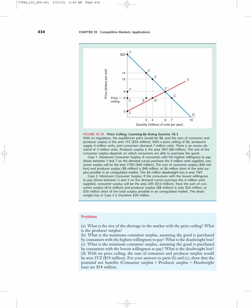
Let’s begin by studying the effects of a minimum wage law. There are manytypes of labor in an economy. Some workers are unskilled, while others are highlyskilled. For most types of skilled labor, the minimum wage set by the governmentwill be well below the equilibrium wage rate in a free market. A minimum wagelaw will have no effect in such a market. We therefore focus on the market forunskilled labor, where the minimum wage requirement is above the wage level ina free market.
Figure 10.11 illustrates the supply and demand curves in the market for un-skilled labor. The vertical axis shows the price of labor, that is, the wage rate, w.The horizontal axis measures the number of hours of labor, L. The supply curve
80 115100
Z
wmin = $6
$5w* = $5
w, w
age
rate
(do
llars
per
hou
r)
T
S
D
V
WF
E
A
G
Y
R
BC
Excess labor supply
L, quantity of labor (millions of hours per year)
FIGURE 10.11 Minimum Wage Law (Minimum Deadweight Loss)A minimum wage law requires employers to pay at least $6 per hour. At that wage rateworkers would like to supply 115 million hours, but employers will only hire workers for80 million hours. The minimum wage law causes an excess supply of labor of 35 millionhours. Because there is an excess supply of labor, it is not clear which workers who wantjobs will be hired. If the most efficient workers (those located between points Z and W onthe supply curve) supply the 80 million hours, the welfare loss from the minimum wagelaw is B � C.
With Impact ofFree Mark Minimum Wage Rent Control
Consumer surplus A � B � G G � A � B
Producer surplus C � E � F A � E � F A � C
Net benefits A � B � C � A � E � F � G � B � C(Consumer � Producer surplus) E � F � G
Deadweight loss zero B � C
7784d_c10_409-461 5/23/01 6:49 AM Page 436

10.5 Price Floors (Minimum Price Regulation) 437
shows how many hours workers will supply at any wage rate. The demand curveindicates how many hours of labor employers will hire.
Suppose a minimum wage law requires employers to pay at least $6 per hour.With no minimum wage law, the market would clear. At the equilibrium wage rateof $5 per hour, workers would supply 100 million hours, just the amount em-ployers want to hire. With the minimum wage law, employers wish to hire only80 million hours (point R ), reducing the demand for labor by 20 million hours.
But the full measure of unemployment is more than 20 million hours. Unem-ployment measures the amount of labor workers would like to supply, but cannotsupply because labor is in excess supply. At the minimum wage of $6 per hour, work-ers would like to supply 115 million hours, but employers will only hire workers for80 million hours. Thus, the minimum wage law causes an excess supply of labor (un-employed labor) of 35 million hours (the horizontal distance between R and T ).
With the minimum wage law the employers who hire labor are the ones be-tween points Y and R on the demand curve. The consumer surplus they receive(remember, employers are the consumers of labor) is area G. Thus, consumer sur-plus falls (by areas A and B) with the minimum wage. This explains why businessesoften strongly lobby policy makers to keep the minimum wage from being raised.
Workers who are lucky enough to get jobs with the minimum wage will re-ceive $6 instead of $5 per hour. The extra income to these workers is measuredby area A. This is an income transfer because it represents money transferredaway from employers to workers. Observe that area B is not part of the incometransfer. Because the minimum wage reduces the number of jobs, the benefits inarea B simply disappear, becoming part of the deadweight loss.
How will producer surplus be affected by a minimum wage law? To answerthis question, we must recognize that all of the suppliers of labor between Z andT on the supply curve want to work at the minimum wage, but only some of themwill find jobs. Since there is an excess supply of labor, we need to know who findsa job. Let’s consider two possible scenarios.
• Case 1. The most efficient workers find jobs. Suppose the workers between Zand W on the supply curve are the ones who find jobs. The other workers between W and T are unable to do so, even though they are willing to workat $6 per hour.
The producer surplus is area A � E � F. This is the maximum possible pro-ducer surplus under the minimum wage. As Figure 10.11 indicates, the sum ofconsumer and producer surplus is A � E � F � G. The deadweight loss is B � C.
• Case 2. The least efficient workers find jobs. A second possibility is that the 80 millionhours are supplied by those workers between points X and T on the supply curvein Figure 10.12.9 The other potential workers between Z and X would be unableto find jobs, even though they are willing to work at a wage of $6 per hour.
Now the producer surplus is area M � N � J. This is the minimum possibleproducer surplus. As Figure 10.12 indicates, the sum of consumer and producer sur-plus is G � J � L � M � N. The minimum wage law creates a deadweight loss of
9We do not consider workers to the right of point T on the supply curve because they would not bewilling to take jobs at a wage of $6 per hour.
7784d_c10_409-461 5/23/01 6:49 AM Page 437

438 CHAPTER 10 Competitive Markets: Applications
A � E � J. The deadweight loss is larger in Case 2 than in Case 1 because the pro-ducer surplus is smaller when inefficient workers displaced more efficient workers.
The two cases define upper and lower limits on the producer surplus anddeadweight loss from a minimum wage law. The actual producer surplus anddeadweight loss may well be in between the levels in these two polar cases, de-pending on which workers find the available jobs.
There are several simplifying assumptions that are important in the analysisof minimum wage laws. First, we assume that the quality of labor does not changeas the minimum wage rises. It is sometimes suggested that employers are able tohire better workers at high wages. If this is the case, the analysis would need torecognize that the supply curve shifts as the wage rate rises, because the quality
11535 100
ZX
wmin = $6
$5w* = $5
w, w
age
rate
(do
llars
per
hou
r)T
S
D
VE
A
G
L
N
M J
Excess labor supply
L, quantity of labor (millions of hours per year)
FIGURE 10.12 Minimum Wage Law (Maximum Deadweight Loss)Since minimum wage law creates an excess supply of labor, it is not obvious which work-ers will find jobs. If the least efficient workers (those located between points X and T onthe supply curve) find jobs, the deadweight loss from the minimum wage law is A � E � J.The welfare loss from the minimum wage law will be larger than in Figure 10.11 becauseproducer surplus is smaller when inefficient workers displace more efficient workers.
With Impact ofFree Market Minimum Wage Rent Control
Consumer surplus A � G � L � M G � L � A � M
Producer surplus E � N M � N � J M � J � E
Net benefits A � E � G � G � J � L � M � N J � A � E(Consumer � Producer surplus) L � M � N
Deadweight loss zero A � E � J
7784d_c10_409-461 5/23/01 6:49 AM Page 438

10.5 Price Floors (Minimum Price Regulation) 439
of labor is not constant. Also, a minimum wage control in one market may affectwage rates in other markets, ultimately affecting the prices of many goods andservices. A study of these additional effects is beyond the scope of the analysishere, but you should recognize that these effects may be important.
EXAMPLE 10.4Unintended Consequences of Price Regulation in Airline Markets
Between 1938 and 1978 the Civil Aeronautics Board (CAB) controlled many keyfeatures of the interstate airline market, including air fares and the number of car-riers in city-pair markets. Regulators required all carriers serving a given interstatecity-pair market (e.g., the route between Chicago and Los Angeles) to charge thesame fare. The CAB also made it difficult for new firms to enter the market.
Although the CAB closely regulated service in interstate markets, it did not havethe authority to regulate airline service in intrastate markets. In unregulated in-trastate markets (for example, on the route between San Francisco and Los Ange-les), the fares were as much as 45 percent lower than on a route of comparabledistance in a regulated interstate market.
Figure 10.13 illustrates the cost difference for two carriers in comparable mar-kets (e.g., in two routes of 400 miles with similar demand curves). The fare in theinterstate market is PREG, while the fare in the unregulated intrastate route is PUNREG.There was little producer surplus in interstate and interstate markets. Unregulatedprice competition and relatively easy entry dissipated profits in intrastate markets.
Profits were also low in interstate markets, but for different reasons. Because ofCAB regulation, interstate carriers were not able to engage in price competition. Theywere also unable to restructure their routes to reduce costs. Without strong pricecompetition, labor unions were often able to win large wage increases. Althoughprices were regulated, carriers competed away almost all of their profits with nonpricecompetition, attempting to attract more passengers by serving expensive meals, hav-ing more flight attendants, and providing other amenities to passengers. Airlines alsocompeted by offering more frequent flights, often leading to low “load factors,” mean-ing that planes typically departed with a high percentage of empty seats.
As Figure 10.13 suggests, the consumer surplus for a comparable route wasmuch higher in an intrastate market (area A � B � G) than in an interstate market(area G). If the costs for interstate carriers had been as low as the costs in intrastatemarkets, airlines would have earned a producer surplus equal to area A, and thedeadweight loss from regulation would have been area B. However, because of non-price competition, interstate airlines did not capture A as producer surplus. Laborunions did capture part of area A with higher wages, and the rest of the potentialeconomic benefit disappeared because of inefficiencies in airline operations.
After deregulation occurred in interstate markets, real (deflated) airline faresdropped significantly, and performance in interstate markets more closely resem-bled that already observed in intrastate markets.10 �
10For more on airline deregulation see E. Bailey, D. Graham, and D. Sibley, Deregulating the Airlines,(Cambridge, Mass., MIT Press, 1985), and S. Borenstein, “The Evolution of U.S. Airline Competition,”Journal of Economic Perspectives, 6 (2) (Spring 1992).
7784d_c10_409-461 5/23/01 6:49 AM Page 439

440 CHAPTER 10 Competitive Markets: Applications
Passenger-miles
PREG
QREG QDEREG
PUNRE
Cos
t (do
llars
per
pas
seng
er m
ile)
Y
G
A B
D
Passenger-miles
(b) The market(a) The individual firm
PREG
PUNRE
Cos
t (do
llars
per
pas
seng
er m
ile)
AC, intrastatemarket
AC, interstatemarket
FIGURE 10.13 Minimum Price Regulation for AirlinesBefore 1978 the Civil Aeronautics Board controlled many key features of the interstate air-line market, including airline fares (PREG). Intrastate airline markets were unregulated(PUNREG), with costs and fares as much as 45 percent lower than fares in comparable regu-lated markets. The consumer surplus for a comparable route was much higher in an in-trastate market (area A � B � G) than in an interstate market (area G). If the costs for in-terstate carriers had been as low as the costs in intrastate markets, airlines would haveearned a producer surplus equal to area A, and the deadweight loss from regulationwould have been area B. However, because of nonprice competition, interstate airlines didnot capture A as producer surplus. Labor unions captured part of area A with higherwages, and the rest of potential economic benefit disappeared because of inefficiencies inairline operations.
E
S
D
LEARNING-BY-DOING EXERCISE 10.4
Price Floor
The supply and demand curves illustrated in Figure 10.14 are the same oneswe have used in the previous three Learning-By-Doing Exercises. With noprice floor, the sum of consumer and producer surplus would be area YVZ($54 million). Suppose the government sets a price floor of $12 in the market.
Problem
(a) What is the size of the excess supply in the market with the price floor?What is the consumer surplus?
7784d_c10_409-461 5/23/01 6:49 AM Page 440

10.5 Price Floors (Minimum Price Regulation) 441
(b) What is the maximum producer surplus, assuming producers with the low-est costs sell the good? What is the deadweight loss?(c) What is the minimum producer surplus, assuming producers with the high-est costs sell the good? What is the deadweight loss?(d) For your answers to parts (b) and (c), show that the potential net benefits(Consumer surplus � Producer surplus � Deadweight Loss) are $54 million.
Solution If the price floor is $12, consumers will demand 4 million units, butproducers will want to supply 10 million. The excess supply is 6 million units,the distance between T and N.
The consumer surplus is the area of the triangle above the price floor of$12 and below the demand curve. Consumer surplus will be the area RTY ($16million).
Pric
e (d
olla
rs p
er u
nit)
Y
T
W
N
Z
AV
M
Quantity (millions of units per year)
6
Supply
Demand
4 10
Pricefloor
2
6
8
12
$20
R
FIGURE 10.14 Price Floor: Learning-By-Doing Exercise 10.4With a price floor of $12, producers would like to supply 10 million units, but con-sumers demand only 4 million units. There is an excess supply of 6 million units. Con-sumer surplus is the area RTY ($16 million). The size of the producer surplus dependson which suppliers are in the market.
Case 1. Maximum Producer Surplus: If producers with the lowest costs (those be-tween Z and W on the supply curve) supply the 4 million units consumers desire, pro-ducer surplus will be the area ZWTR ($32 million). The sum of consumer surplus ($16million) and producer surplus ($32 million) is $48 million, or $6 million short of the to-tal surplus possible in an unregulated market. This $6 million deadweight loss is areaTWV.
Case 2. Minimum Producer Surplus: If producers with the highest costs (those be-tween V and N on the supply curve) supply the 4 million units, producer surplus will bethe area MNV ($8 million). The sum of consumer surplus ($16 million) and producersurplus ($8 million) is only $24 million, or $30 million short of the total surplus possiblein an unregulated market. The deadweight loss in Case 2 is therefore $30 million.
7784d_c10_409-461 5/23/01 6:49 AM Page 441

442 CHAPTER 10 Competitive Markets: Applications
Suppose that the most efficient producers (those between Z and W on thesupply curve) supply the 4 million units consumers desire. Producer surpluswill be the area ZWTR ($32 million). The sum of consumer surplus ($16 mil-lion) and producer surplus ($32 million) is $48 million.
How much is the deadweight loss? With the price floor the consumer andproducer surplus is only $48 million, or $6 million short of the total surpluspossible in an unregulated market. This $6 million deadweight loss is area TWV.
If least efficient suppliers (those between V and N on the supply curve) sellthe 4 million units, producer surplus will be the area MNV ($8 million). Nowthe sum of consumer surplus ($16 million) and producer surplus ($8 million)is only $24 million, or $30 million short of the total surplus possible in an un-regulated market ($54 million). The deadweight loss in Case 2 is $30 million.
For part (b): Consumer surplus ($16 million) � Producer surplus ($32 mil-lion) � Deadweight loss ($6 million) � $54 million.
For part (c): Consumer surplus ($16 million) � Producer surplus ($8 mil-lion) � Deadweight loss ($30 million) � $54 million.
Once again, this exercise shows that potential surplus is the same with andwithout government intervention. When consumers and producers fail to cap-ture potential surplus, it becomes a deadweight loss.
Similar Problem: 10.7
If the government wants to support the price at a level above the equilibriumprice in a free market, it may restrict the quantity produced. To limit the quan-tity produced, the government may place a quota, or a limit, on the number ofproducers in the market, or on the amount that each producer can sell. A quotaattempts to place a ceiling on the quantity that producers can supply.
We have historically observed quotas in many agricultural markets. For ex-ample, the government may limit the number of acres a farmer can plant. Quo-tas are used in other industries, too. In many cities governments limit the num-ber of taxis that may be operated, often leading to fares higher than those thatwould be observed in unregulated markets.
When the government imposes a quota in a market with an upward-slopingsupply-curve and a downward sloping demand curve, it results in the following:
• The market will not clear. There will be an excess supply of the good or serv-ice in the market.
• Consumers will buy less of the good than they would in a free market.• Consumer surplus will be lower than would be the case with no quota.• Some (but not all) of the lost consumer surplus will be transferred to producers.• Because there is excess supply with a quota, the size of the producer surplus
depends on which of the producers who want to supply the good are able todo so. If the most efficient suppliers serve the market, a quota may increaseproducer surplus.11
10.6PRODUCTION
QUOTAS
11We say that producer surplus may increase. If the most efficient producers serve the market, producersurplus will increase for some levels of the quota. However, of the quota is too low (for example, closeto zero), producer surplus could actually decrease.
7784d_c10_409-461 5/23/01 6:49 AM Page 442

10.6 Production Quotas 443
Figure 10.15 illustrates the effects of a quota. With no quota, the equilibriumprice is $8, and the sum of consumer and producer surplus is area A � B � C �E � F ($54 million).
The demand curve indicates that consumers will pay $12 per unit when aquota limits production to 4 million units. At that price producers would like tosupply 10 million units. There will be an excess supply of 6 million units.
With a quota, consumer surplus (area F, $16 million) is lower than the amountin the competitive market (areas A � B � F, $36 million). The reduction in
Pric
e (d
olla
rs p
er u
nit)
Quantity (millions of units per year)
64 10
2
6
8
12
$20
F
A
EC
B
S
D
FIGURE 10.15 Production QuotaIf a quota limits production to 4 million units, consumers pay a price of $12. Producerswould like to supply 10 million units at that price. There is therefore an excess supply of 6million units. Consumer surplus is the area F ($16 million). The size of the producer sur-plus depends on which suppliers are in the market. In this example we assume producerswith the lowest costs supply the 4 million units consumers desire. Producer surplus is thearea A � E ($32 million). The sum of consumer surplus ($16 million) and producer surplus($32 million) is $48 million, or $6 million short of the total surplus possible in an unregu-lated market. This $6 million deadweight loss is area B � C.
Free Market With(No Quota) Quota Effect of Quota
Consumer surplus A � B � F F �A � B($36 million) ($16 million) (�$20 million)
Producer surplus C � E A � E �A � C($18 million) ($32 million) ($14 million)
Net benefits A � B � C � E � F A � E � F �B � C(Consumer � Producer surplus) ($54 million) ($48 million) (�$6 million)
Deadweight loss zero B � C($6 million)
7784d_c10_409-461 5/23/01 6:49 AM Page 443

444 CHAPTER 10 Competitive Markets: Applications
consumer surplus occurs because the quota supports the price at $12, well abovethe $8 equilibrium price in a competitive market.
The size of the producer surplus depends on which suppliers are in the mar-ket. If producers with the lowest costs serve the market, producer surplus is the area A � E ($32 million). The sum of consumer surplus ($16 million) andproducer surplus ($32 million) is $48 million, $6 million short of the total sur-plus possible in an unregulated market. This $6 million deadweight loss is areaB � C.
Finally, because producers would like to supply 10 million units when theprice is $12, there is no guarantee that the most efficient producers will supplythe 4 million units allowed by the quota. The 4 million units might be suppliedby inefficient suppliers, such as those located between the quantities of 6 millionand 10 million units on the supply curve. Then producer surplus will be muchlower ($8 million). You should verify this, and also show that the deadweight losscould be as high as $30 million.
EXAMPLE 10.5 Quotas for Taxi Cabs
The taxi cab industry has the features of a competitive market. There are manysmall consumers of taxi service, and, if entry were unregulated, there would alsobe many firms providing service. However, in many cities in the world, taxis areregulated. Sometimes government control takes the form of direct price regulation.More often, cities restrict the number of licenses authorizing a taxi to operate onthe street. Historically, the licenses have often been metallic objects (calledmedallions) issued by the government to certify that the driver has permission toprovide taxi service. These days, a medallion is often just a paper document.
It is not surprising that taxi fares are substantially higher in cities with quotasthan in cities that allow free entry because the number of medallions limits the sup-ply of taxis. For example, in Washington, D.C., it is quite easy to enter the market,and fares are low, often half as high as they are in cities with quotas.
There are usually active markets that enable the owner of a medallion to sell itto other prospective drivers. If you want to operate a taxi in a market with a quota,you can buy an existing medallion from someone who has one. Because the quotassupport the price above the equilibrium level, the medallions can be quite valuable.For example, in New York City, a taxi medallion was worth about $230,000 in 1999.
When medallions can be sold, a more efficient supplier will be willing to paymore for a medallion than a less efficient supplier. The suppliers of taxi service arelikely to be those with the lowest costs. This suggests that the deadweight loss fromthe quota system will be at the lower end of the theoretically possible range. If thesupply and demand curves are similar to those in Figure 10.15, the deadweight lossshould be near the area B � C.
In recent years many cities have been increasing the number of medallions overtime, making the market more competitive. For example, early in the 1980s, thecity of Chicago had a restrictive quota system with only two major suppliers of taxiservice (Yellow and Checker). The city government initiated a program to increasethe number of medallions gradually over a number of years.
7784d_c10_409-461 5/23/01 6:49 AM Page 444

10.6 Production Quotas 445
The political reasons for the move toward competition are interesting. As thenumber of medallions increases, the value of medallions will fall. Owners of medal-lions often form a powerful interest group, strenuously objecting to increasing thenumber of medallions. However, there are also strong interests in favor of entry.People with low incomes frequently use taxi service, and they are strongly in favorof the program to increase competition. Politicians understand that customers oftaxi service will benefit from lower fares, and these taxi customers are voters. In theend, in Chicago the voters carried the day, sending the move toward more com-petition on its way.
One might ask why the City of Chicago did not deregulate taxis all at once by simply eliminating the need for medallions. Out of fairness to existingholders of medallions, the government phased in increased entry over time. Any-one who bought a medallion just before the program of increased entry was an-nounced paid a handsome price for it. By phasing in the program over a numberof years, the program allowed existing holders to recover much of their invest-ment in medallions. �
E
S
D
LEARNING-BY-DOING EXERCISE 10.5
Comparing a Tax, Minimum Price Regulation, and a Quota
Before going further, let’s take a moment to compare three types of govern-ment intervention that lead consumers to pay a price higher than the free mar-ket price. Throughout this chapter we have used the supply and demand curvesin Figure 10.1 to study the effects of government intervention. We have foundthat the price consumers pay will be $12 per unit for each of the followingforms of intervention:
1. An excise tax of $6 (Learning-By-Doing Exercise 10.1)2. A price floor of $12 (Learning-By-Doing Exercise 10.4)3. A quota of 4 million units (Figure 10.15)
To review and compare the results of these examples, answer the follow-ing questions:
Problem
(a) How will consumer surplus differ?(b) For which of the forms of intervention will we expect the producers in themarket to be the efficient suppliers (the ones at the lower end of the supplycurve)?(c) Which type (or types) or government intervention might producers prefer?(d) Which type (or types) of government intervention lead to the lowest dead-weight loss?
7784d_c10_409-461 5/23/01 6:49 AM Page 445

446 CHAPTER 10 Competitive Markets: Applications
Solution
(a) Since the price charged to consumers is $12 with each type of interven-tion, consumer surplus is the same.(b) Since the market clears with an excise tax, the suppliers in the market willbe the efficient ones. The market does not clear with a price floor or a quota.Inefficient suppliers may serve the market. However, if the quota is implementedwith a certificate that authorizes production (as with taxi medallions in Exam-ple 10.5), and if the certificates can be resold in a competitive market, then wewould expect the suppliers who ultimately acquire the certificates to be efficient.(c) Producers would prefer the price floor or the quota, both of which mayincrease producer surplus. Producers will least prefer the excise tax because thetax will reduce producer surplus.(d) Since the price and output levels are the same with all three forms of in-tervention, the deadweight loss will be smallest when there are efficient pro-ducers in the market (and the conditions under which efficient producers willserve the market are summarized in part (b)).
This exercise helps us to appreciate why programs that have a common con-sequence (here, the price consumers pay) may still differ substantially in otherways. For example, a higher consumer price does not necessarily mean thatproducers are better off, or that alternative programs are equally efficient. Fur-thermore, people who do not consume the good may benefit if tax revenuescollected in this market can be used to reduce tax burdens elsewhere.
As noted in the introduction to this chapter, price support programs are commonin the agricultural sector. These programs typically increase producer surplus forthe farmers. In the United States, supports for products such as soybeans, corn, andpeanuts often hold prices above their free market levels. Because price support pro-grams are expensive to taxpayers, many governments have reduced price supportprograms over the last decade. However, many programs remain in place, and some-times enjoy a resurgence in years when low prices threaten farming incomes.
In this section we describe two price support programs that have been usedin the agricultural sector, acreage limitation programs and government purchaseprograms.
With an acreage limitation program, the government gives farmers an in-centive to hold production below the free market level. Figure 10.16 illustrateshow such a program works, using supply and demand curves similar to those inFigure 10.1. (We have labeled the horizontal axis in billions of bushels becauseagricultural support programs often involve billions instead of millions of dol-lars.) In equilibrium farmers produce 6 billion bushels per year.
Suppose the government wants to support a price of $10 per bushel. Insteadof imposing a quota, it provides farmers with an incentive to reduce output to 5billion bushels, the level that would lead consumers to pay a price of $10. At a priceof $10, farmers would like to produce 8 billion bushels. They would be willing toproduce only 5 billion bushels only if the government compensates them for notproducing the additional 3 billion bushels they would like to supply. The amount
10.7OTHER PRICE
SUPPORTS
7784d_c10_409-461 5/23/01 6:49 AM Page 446

10.7 Other Price Supports 447
Pric
e (d
olla
rs p
er b
ushe
l)
Quantity (billions of bushels per year)
6 8 105
Supportprice
2
8
10
$20
F
A
E
CB G
S
D
FIGURE 10.16 Acreage Limitation ProgramSuppose the government wants to support a price of $10 per bushel. Instead of imposinga quota, the government offers farmers cash for planting less acreage, reducing output to 5 billion bushels. At a price of $10, farmers would like to produce 8 billion bushels.They would be willing to produce only 5 billion bushels if the government compensatesthem for not producing the additional 3 billion bushels. They require a payment equal to area B � C � G, the amount of producer surplus they forgo if they plant only 5 billionbushels. The program costs the government $4.5 billion, and increases producer surplusby $14 billion. The net benefit to society is the sum of consumer surplus ($25 billion) and producer surplus ($32 billion), less the cost to the government ($4.5 billion), resulting in a net benefit of $52.5 billion and a deadweight loss of $1.5 billion (area B � C ).
With Acreage Limitation Effect ofFree Market Program Program
Consumer surplus A � B � F F �A � B($36 billion) ($25 billion) (�$11 billion)
Producer surplus C � E A � B � C � E � G A � B � G($18 billion) ($32 billion) ($14 billion)
Impact on treasury zero �B � C � G �B � C � G(�$4.5 billion) (�$4.5 billion)
Net benefits A � B � C � E � F A � E � F �B � C(Consumer � Producer surplus ($54 billion) ($52.5 billion) (�$1.5 billion)� Impact on Treasury)
Deadweight loss zero B � C($1.5 billion)
7784d_c10_409-461 5/23/01 6:49 AM Page 447

448 CHAPTER 10 Competitive Markets: Applications
of producer surplus farmers would forgo to limit production is equal to area B �C � G. This is the payment they will require to participate in the program.
The program increases producer surplus by $14 billion (A � B � G). It coststhe government $4.5 billion (B � C � G). The net benefit to society is the sumof consumer surplus ($25 billion) and producer surplus ($32 billion), less the costto the government ($4.5 billion), or $52.5 billion. The deadweight loss is $1.5billion (B � C).
Since the program introduces a deadweight loss, one might ask why the gov-ernment does not simply give farmers a cash transfer of $14 billion, and then letthe market function without intervention to produce 6 billion bushels at a priceof $8. This might seem attractive because the deadweight loss would then be zero.The government would collect the money to pay for the program from taxes im-posed elsewhere. Although such a program would be efficient, the public mayfind it more palatable to pay farmers $4.5 billion to reduce output (and forego aprofit opportunity) than to give farmers $14 billion to do nothing at all.12
As in alternative to an acreage limitation program, the government can sup-port the price with a government purchase program. Figure 10.17 illustrates howsuch a program might work. At a price of $10 per bushel farmers would like toproduce 8 billion bushels. The market demand would be only 5 billion bushelsat that price. There would be an excess supply of 3 billion bushels.
To maintain a price of $10 per bushel, the government could buy 3 billionbushels to eliminate the excess supply. Producer surplus increases by $14 billion(A � B � G).
How much would the program cost the government? The government mustpurchase the excess supply (3 billion bushels) at a price of $10 per bushel. Thecosts to the government is thus $30 billion (area B � C � G � H � I � J ). Thegovernment could reduce the cost of the program if it were to sell some of thecommodity somewhere in the world, even at a low price to help countries in need.However, if it releases some of the commodity into the market, it must recog-nize that it could drive the price down, lowering farmers’ producer surplus,thereby working against the original goal of the support program.
The net benefit to society is the sum of consumer surplus ($25 billion, areaF ) and producer surplus ($32 billion, area A � B � C � E � G), less the cost tothe government ($30 billion). The program results in a net benefit of $27 billionand a deadweight loss of $27 billion (area B � C � H � I � J ).
E
S
D
LEARNING-BY-DOING EXERCISE 10.6
Comparing Price Support Programs: Government Purchasesand Acreage Limitations
This exercise will help you compare the two price support programs we havejust discussed, the acreage limitation program illustrated in Figure 10.16 andthe government purchase program depicted in Figure 10.17. The labels in the
12Of course, we must recognize that the government may create deadweight losses in other marketswhen it imposes taxes to raise the $14 billion to pay for the acreage limitation program.
7784d_c10_409-461 5/23/01 6:49 AM Page 448
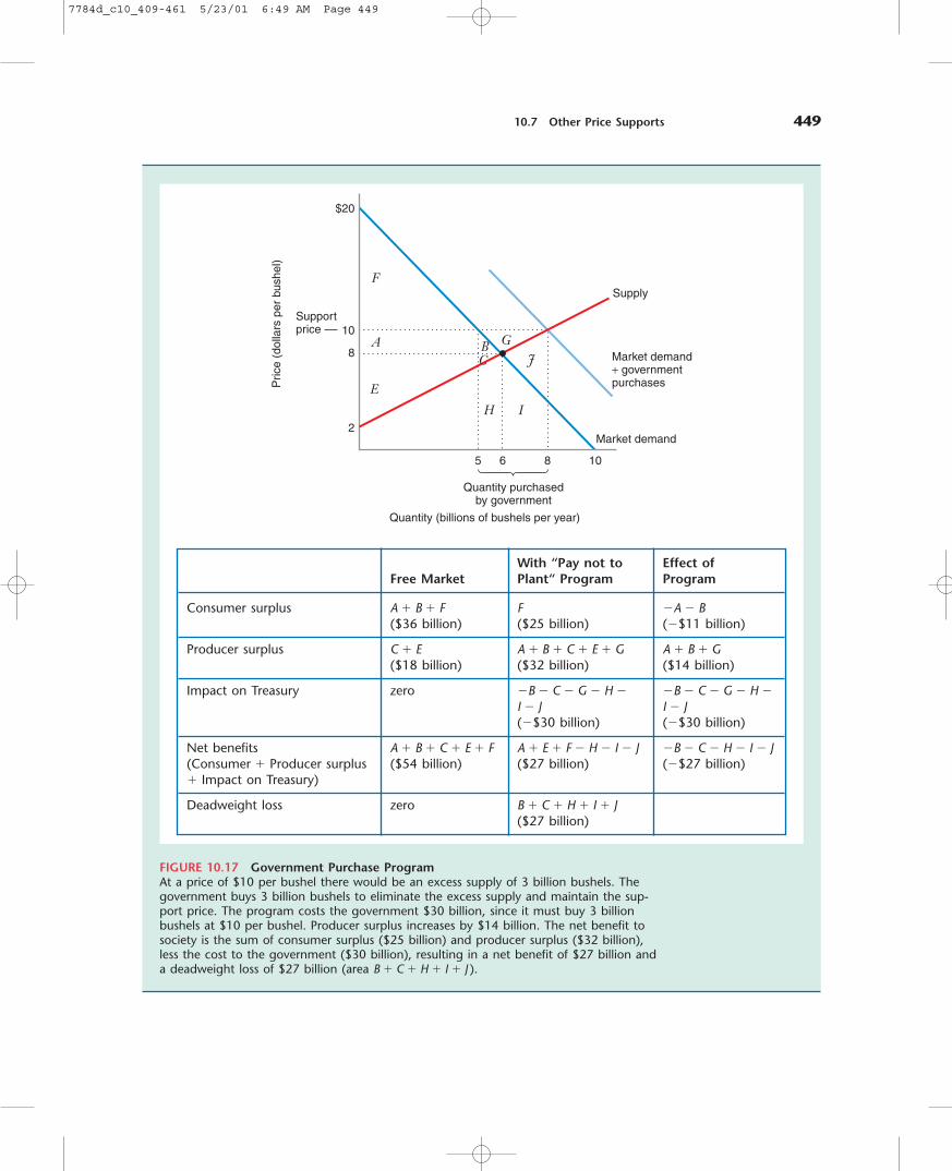
10.7 Other Price Supports 449
Pric
e (d
olla
rs p
er b
ushe
l)
Quantity (billions of bushels per year)
Quantity purchasedby government
6
Market demand+ governmentpurchases
Supply
Market demand
8 105
Supportprice
2
8
10
$20
F
A
E
C
H I
JB G
FIGURE 10.17 Government Purchase ProgramAt a price of $10 per bushel there would be an excess supply of 3 billion bushels. Thegovernment buys 3 billion bushels to eliminate the excess supply and maintain the sup-port price. The program costs the government $30 billion, since it must buy 3 billionbushels at $10 per bushel. Producer surplus increases by $14 billion. The net benefit tosociety is the sum of consumer surplus ($25 billion) and producer surplus ($32 billion),less the cost to the government ($30 billion), resulting in a net benefit of $27 billion anda deadweight loss of $27 billion (area B � C � H � I � J ).
With “Pay not to Effect ofFree Market Plant“ Program Program
Consumer surplus A � B � F F �A � B($36 billion) ($25 billion) (�$11 billion)
Producer surplus C � E A � B � C � E � G A � B � G($18 billion) ($32 billion) ($14 billion)
Impact on Treasury zero �B � C � G � H � �B � C � G � H �I � J I � J(�$30 billion) (�$30 billion)
Net benefits A � B � C � E � F A � E � F � H � I � J �B � C � H � I � J(Consumer � Producer surplus ($54 billion) ($27 billion) (�$27 billion)� Impact on Treasury)
Deadweight loss zero B � C � H � I � J($27 billion)
7784d_c10_409-461 5/23/01 6:49 AM Page 449
450 CHAPTER 10 Competitive Markets: Applications
areas in the two figures correspond to one another (for example, area B is thesame in both figures). Use the labels in the areas in the two figures to answerthe following questions:
Problem
(a) If the two programs support the same price in a market, which programwill cost the government more?(b) Which program will create a larger deadweight loss?(c) Which program would farmers prefer?
Solution
(a) The cost to the government with an acreage limitation program is area B � C � G. The cost with government purchase program is B � C � G � H� I � J. Thus, the government purchase program is more costly.(b) The deadweight loss with an acreage limitation program is area B � C �G. The deadweight loss with government purchase program is B � C � G �H � I � J. Thus, the deadweight loss is greater with the government purchaseprogram.(c) Farmers are indifferent since they receive the same addition to producersurplus (A � B � G) under either program.
Government purchase programs are more costly and less efficient thanacreage limitation programs.13 Often a government must spend much morethan one dollar to increase farmers’ producer surplus by a dollar. Neverthe-less, many countries resort to government purchase programs, and they aregenerally more palatable politically than direct cash payments to farmers.
Many countries impose tariffs and quotas on imports to help support the priceof a good in the domestic market, especially when the price in world market isquite low and unrestricted imports would hurt domestic producers. Tariffs andquotas lead to higher domestic prices, enabling domestic producers to expandproduction and earn higher levels of producer surplus. In this section we will seethat tariffs and quotas help domestic producers and reduce domestic consumersurplus. We will also show that these forms of intervention lead to deadweightlosses by diminishing the level of total domestic surplus.
Consumers in a country will import a good when the world price of the goodis below the equilibrium price that would be observed in the domestic market ifthere were no imports. In Figure 10.18 the domestic supply and demand curvesindicate that the equilibrium price in the market would be $8 if there were nointernational trade. At that price 6 million units would be produced and sold in
10.8IMPORT
TARIFFS ANDQUOTAS
13If we think in terms of general equilibrium, the government purchase program in one sector is likelyto create even more deadweight loss in other sectors of the economy because larger taxes will have to becollected elsewhere to finance the program.
7784d_c10_409-461 5/23/01 6:49 AM Page 450

10.8 Import Tariffs and Quotas 451
Pric
e (d
olla
rs p
er u
nit)
Quantity (millions of units per year)
Imports with free trade(no tariff or quota)
Q2 = 6No trade
Q1 = 2Domesticsupply,freetrade
Q3 = 8Domesticdemand,freetrade
Foreign supply (world price)
Domestic supply
Domestic demand
10
2
8
Pw = 4
$20
F
A CB
G
FIGURE 10.18 Imports with Free TradeIf trade were not allowed, the intersection of the domestic supply and demand curvesdetermines the equilibrium in the domestic market, leading to a price of $8 and a quan-tity of 6 million units. If the trade prohibition is removed (free trade is allowed), thegood can be imported at a price of $4. The domestic price will be $4 because no do-mestic consumer need pay more than that price. Domestic production will fall to Q1. Theamount consumed domestically is Q3. Imports are the difference between domestic con-sumption (Q3) and domestic production (Q1). Domestic consumers benefit (their con-sumer surplus increases by A � B � C ). But domestic producers find their producer sur-plus reduced by area A. A prohibition on trade reduces total domestic surplus by B � C,the deadweight loss.
Effect of TradeFree Trade No Trade Prohibition
Consumer surplus A � B � C � F F �A � B � C
Producer surplus G A � G A
Net benefits (Domestic) A � B � C � F � G A � F � G �B � C(Consumer � Producer surplus)
Deadweight loss zero B � C
7784d_c10_409-461 5/23/01 6:49 AM Page 451

452 CHAPTER 10 Competitive Markets: Applications
the market, and the domestic market would clear. Domestic consumer surpluswould be area F, and domestic producer surplus would be A � G. Thus, the sumof domestic consumer and producer surplus would be area A � F � G.
Now suppose that the good could be purchased on the world market at aprice of $4. Since this price is below the equilibrium price in the domestic mar-ket with no trade, domestic consumers will want to import the good. With freetrade, the equilibrium price in the domestic market will become $4 because nodomestic consumer ever needs to pay more than that price to purchase the good.
What are the consequences of free trade in the domestic market? At a priceof $4, domestic consumers would purchase Q3 (8 million units per year). At thatprice domestic producers would only be willing to supply Q1 (2 million units).The amount imported would therefore be the difference between the quantitydemanded and the quantity supplied domestically, or (Q3 � Q1), that is, 6 millionunits per year. Consumer surplus with free trade will be A � B � C � F. Becausedomestic production has fallen with free trade, domestic producers will have asurplus of G.
As the graph indicates, domestic producers in this industry will be unhappyabout free trade. Because domestic production falls with free trade, domestic pro-ducers will benefit from a prohibition on free trade, gaining the additional pro-ducer surplus A.
Since domestic producers stand to lose with free trade, they often attempt torestrict or even eliminate imports. Let’s suppose that they succeed in lobbyingCongress to eliminate free trade altogether. The consequences of this policy aresummarized in the table below the graph in Figure 10.18. As already noted, do-mestic producers would increase their surplus by A. Consumers would lose A �B � C because the price would increase to $8. As a whole, net benefits to soci-ety would decrease by B � C, the deadweight loss from prohibition.
A government may also eliminate imports if it imposes a large enough tariff on the good. A tariff is a tax on imported good. If the world price is $4 andthe government charges a tariff of $5, a domestic consumer would have to pay$9 to buy the imported good. But no consumer would buy an imported good be-cause it would be available for $8 in the domestic market if there were no trade.In other words, if the tariff is at least as large as the difference between the do-mestic price with no trade and the world price, nothing will be imported. In theexample in Figure 10.18, no imports will occur if the tariff is larger than $4.
What happens if a tariff less than $4 is imposed? For example, suppose a tar-iff of $2 is levied on the good. Figure 10.19 illustrates the equilibrium with thetariff. Domestic consumers will now be able to buy the imported good for $6,the payment required to cover the world price of $4 plus the $2 tariff. Thus, $6will be the price in the domestic market. Since the $6 price is below the $8 pricewith no trade, some imports will occur.
How much will be imported? When the price is $6, consumers will purchaseQ3 (7 million units). At that price domestic suppliers will produce Q2 (4 millionunits). The difference (Q3 � Q2), or 3 million units, will be imported.
How will the imposition of a tariff affect the domestic market? As the tablein Figure 10.19 shows, domestic producers stand to gain from the tariff. Theirproducer surplus increases by the area A. This gain to domestic producers ex-plains why producers often lobby for tariffs.
However, benefits to domestic consumers are reduced. Consumer surplus fallsby A � B � C � H as a result of the tariff.
7784d_c10_409-461 5/23/01 6:49 AM Page 452

Pric
e (d
olla
rs p
er u
nit)
Quantity (millions of units per year)
Imports with no tariff
Imports with tariff
Q1 = 2Domesticsupply,no tariff
Q4 = 8Domesticdemand,no tariff
Q2 = 4Domesticsupply,withtariff
Q3 = 7Domesticdemand,withtariff
Pw + Tariff
Pw = 4
Domestic supply
Domestic demand
10
2
8
6
$20
F
A CH
E
BG
FIGURE 10.19 Import TariffWith free trade the price in the domestic market will be $4, the price at which the goodcan be imported. At that price the amount imported will be the difference between Q4
(the quantity demanded domestically) and Q1 (the quantity supplied by domestic produc-ers). If the government imposes a tariff of $2 per unit, domestic consumers will have topay $6 per unit. The amount imported will be (Q3 � Q2), or 3 million units. The tariff in-creases producer surplus for domestic suppliers by the area A. However consumers lose A � B � C � H. The government collects revenues from the tariff equal to area H. Thus,the domestic deadweight loss is B � C.
Free Trade(No Tariff) With Tariff Effect of Tariff
Consumer surplus A � B � C � E � F � E � F �A � B � C � H
Producer surplus G A � G A
Impact on Treasury zero H H
Net benefits (Domestic) A � B � C � E � A � E � F � G � H �B � C(Consumer � Producer surplus F � G � H� Impact on Treasury)
Deadweight loss zero B � C
Producer surplus, Foreign zero zero zero
453
7784d_c10_409-461 5/23/01 6:49 AM Page 453

454 CHAPTER 10 Competitive Markets: Applications
Pric
e (d
olla
rs p
er u
nit)
Quantity (millions of units per year)
Imports with no quota
Imports with quota
Q1 = 2Domesticsupply,no quota
Q4 = 8Domesticdemand,no quota
Q2 = 4Domesticsupply,withquota
Q3 = 7Domesticdemand,withquota
Pw = 4
Domestic supply
Domestic demand
10
2
8
6
$20
F
A CH
E
BG
FIGURE 10.20 Import QuotaWhen the government restricts imports, the price in domestic market will rise. Suppose aquota limits imports to be no larger than 3 million units (Q3 � Q2). The price in the do-mestic market will be $6. At that price the quantity imported plus the quantity supplieddomestically will equal the quantity demanded by domestic consumers. The quota in-creases producer surplus for domestic suppliers by the area A. However, consumers lose A� B � C � H. The government collects no revenues from a quota, so the area H becomesproducer surplus for foreign suppliers. Thus, the domestic deadweight loss is B � C � H.
No Tariff With Tariff Effect of Tariff
Consumer surplus A � B � C � E � F� E � F �A � B � C � H
Producer surplus G A � G A
Impact on Treasury zero zero zero
Net benefits (Domestic) A � B � C � E � A � E � F � G �B � C � H(Consumer � Producer surplus F � G � H� Impact on Treasury)
Domestic deadweight loss zero B � C � H
Producer surplus, Foreign zero H H
7784d_c10_409-461 5/23/01 6:49 AM Page 454

10.8 Import Tariffs and Quotas 455
There is one further impact of the tariff on the domestic economy. The gov-ernment is collecting revenues from the tariff. The size of that revenue is obtainedby multiplying the tariff ($2 per unit) by the number of units imported, (Q3 � Q2),or 3 million units. In the example, revenues from the tariff would be $6 millionper year, the amount represented by area H in the figure. The area H is a net ben-efit because it can be redistributed to people in the domestic economy.
When we add all of the net benefits from the tariff, we find that domesticbenefits have fallen by B � C, the deadweight loss resulting from the tariff. AreaB is a deadweight loss arising from the overproduction of domestic producerswith the tariff. Area C is a deadweight loss because consumers are purchasingfewer units than they would have at the free market price.
The tariff has reduced imports from 6 million units to 3 million units peryear. As Figure 10.20 illustrates, the government could also raise the domesticprice from $4 to $6 by imposing a quota. A quota sets a maximum on the amountof a good that may be imported.
Suppose the government sets a quota of 3 million units per year in this market.The equilibrium price in the domestic market is the one that clears the market, thatis, makes total supply (domestic and imports) equal to domestic demand. As the graphshows, the equilibrium price will be $6. At that price domestic suppliers will produce4 million units and imports will be 3 million units. This is the amount necessary tosatisfy domestic consumers, who want to purchase 7 million units at a price of $6.
How will the imposition of the quota affect the domestic market? As the tablein Figure 10.20 shows, domestic producer surplus increases by the area A. And,as before, the quota reduces domestic consumer surplus falls by A � B � C � H.
The tariff in Figure 10.19 and the quota in Figure 10.20 lead to the same equi-librium price and level of imports. As the figures show, the impacts of the tariff andquota are the same for consumers and producers. However, there is one importantdifference between the tariff and the quota. With the tariff, the government col-lects area H as revenue from the tariff. As noted earlier, this is a benefit to the econ-omy because these revenues can be redistributed to members of society. With thequota no revenues are collected by the government. Area H becomes a part of pro-ducer surplus for foreign suppliers who are able to sell their goods at a price of $6when they would have been willing to supply at a price of $4. Thus, area H is lostto the domestic economy, and becomes part of the domestic deadweight loss. Whenwe add all of the net benefits from the quota, we find that domestic benefits havefallen by B � C � H, the deadweight loss resulting from the tariff.
Dumping
In the past decade some countries have complained that foreign countries havesubsidized their own industries to help them gain a larger share of the world mar-ket. For example, it has often been alleged that Japanese producers of steel are sell-ing in foreign markets at a price below their cost. In this example we study the ef-fects of dumping.
Suppose that the world price of steel delivered to the United States is PW, set in a competitive world market in which price, average cost, and marginal cost areequal. If a foreign government provides a subsidy of $S per unit, the domestic con-sumers would be able to import steel at a price PW � S, as Figure 10.21 illustrates.
EXAMPLE 10.7
7784d_c10_409-461 5/23/01 6:49 AM Page 455

456 CHAPTER 10 Competitive Markets: Applications
Pric
e (d
olla
rs p
er to
n)
Quantity (millions of tons per year)
Imports with dumping
Imports with no dumping
Q1Domesticsupply,withdumping
Q4Domesticdemand,withdumping
Q2Domesticsupply,with nodumping
Q3Domesticdemand,with nodumping
Pw − S
Pw
Domestic supply
Domestic demand
F
A CH
E
B
G
FIGURE 10.21 DumpingSuppose steel can be produced in the rest of the world and delivered to the United Statesat the price PW. If a foreign government engages in dumping, it is subsidizing its steel in-dustry to help it gain a larger share of the world market. Suppose a foreign governmentgives its steel producers a subsidy of $S per ton. The price to domestic consumers in theUnited States is then PW � S. Imports will expand from (Q3 � Q2) to (Q4 � Q1). Domesticconsumers will benefit as their surplus increases by A � B � C � H � I. However, domesticproducers will be unhappy with the dumping because their surplus falls by A � I. Net do-mestic benefits rise by B � C � H. Part of the increase in domestic benefit results from thesubsidy the foreign government is paying to its producers, B � C � H � I � J.
Free Trade(No Dumping) With Dumping Effect of Dumping
Consumer surplus E � F A � B � C � E � A � B � C � H � IF � H � I
Producer surplus A � G � I G �A � I
Net benefits (Domestic) A � E � F � G � I A � B � C � E � F � B � C � H(Consumer � Producer surplus) G � H � I
Impact on Treasury of zero �B � C � H � I � J �B � C � H � I � JForeign government
7784d_c10_409-461 5/23/01 6:49 AM Page 456

Chapter Summary 457
Under free trade (with no dumping) imports would be Q3 � Q2. However, with thenew, lower domestic price with dumping, imports will expand to Q4 � Q1.
How will dumping affect the domestic market? Domestic consumers will ben-efit as their surplus increases by A � B � C � H � I. However, domestic producerswill be quite unhappy with the dumping because their surplus falls by A � I. Amongother things, they will note that dumping keeps workers on the job in the countryengaging in dumping, while unemployment is likely to rise among steel workers athome. That is why it is often said that dumping leads to an export of jobs from thedomestic country to the country subsidizing its industry.
In practice, it is not easy to establish that dumping is occurring because oneneeds proof that firms are selling at a price below cost. It may be especially diffi-cult to gather data on the costs of production for foreign firms. �
CHAPTER SUMMARY
• In a competitive market each producer acts in its ownself interest, deciding whether to be in the market, and,if so, how much to produce to maximize its own producersurplus. Similarly, each consumer also acts in his or herown self interest, maximizing utility to determine howmany units of the good to buy. Even though there is nosocial planner telling producers and consumers how tobehave, the output in a competitive market maximizes neteconomic benefits (as measured by the sum of the sur-pluses). It is as though there is an “invisible hand” guid-ing a competitive market to the efficient level of pro-duction and consumption.
• Government intervention can take many forms, in-cluding taxes and subsidies, minimum and maximumprice regulation, production quotas, price support pro-grams, and tariffs on imports and exports. For some kindsof government intervention (such as taxes and subsidies)the market will clear. For other types of intervention(such as price ceilings, price floors, and production quo-tas) the market will not clear. When the market does notclear, we must understand who is participating in the mar-ket when we measure consumer and producer surplus.
• When a tax is imposed in a market, the price con-sumers pay usually rises by less than the amount of thetax, and the price producers receive usually falls by lessthan the amount of the tax. The incidence of a tax meas-ures the effect of a tax on the prices consumers pay andsellers receive in a market. When demand is rather in-elastic and supply is relatively elastic, the incidence of anexcise tax will be larger for consumers than for produc-ers. When the magnitudes of the elasticities are reversed,
the incidence of an excise tax will be larger for produc-ers than for consumers.
• Government intervention in competitive marketsusually leads to a deadweight loss. Deadweight loss is aneconomic inefficiency that arises when consumers andproducers do not capture potential net benefits.
• Government intervention in competitive markets of-ten redistributes income from one part of the economyto another. If the government collects revenues throughtaxes or tariffs, the receipts are part of the net benefit tothe economy because the revenues can be redistributed.Similarly, net flows away from the government are a partof the cost of a program.
• An excise tax leads to a deadweight loss because themarket produces less than the efficient level. A tax alsoreduces both consumer and producer surplus. (LBDExercise 10.1)
• When the government pays a subsidy for each unitproduced, the market produces more than the efficientlevel, leading to a deadweight loss. A subsidy increasesboth consumer and producer surplus, but these gains areless than the government’s cost to supply the subsidy.(LBD Exercise 10.2)
• With a binding price ceiling (i.e., a ceiling belowthe free market price), the amount exchanged in themarket will be less than the efficient level because pro-ducers restrict supply. There will be excess demand inthe market, and consumers who value the good the mostmay not be able to purchase the good. (LBD Exer-cise 10.3)
7784d_c10_409-461 5/23/01 6:49 AM Page 457

• With a binding price floor (i.e., a floor above the freemarket price), the amount exchanged in the market willbe less than the efficient level because consumers buyless. There will be excess supply in the market, and thelowest cost producers may not be those who supply thegood. (LBD Exercise 10.4)
• A production quota raises the price consumers payby limiting the output in the market. Although onewould normally expect producer surplus to rise with sucha quota, this need not always occur. Because the marketdoes not clear with a production quota, there is no guar-
antee that the suppliers serving the market are the oneswith the lowest cost. (LBD Exercise 10.5)
• Acreage limitation and government purchase pro-grams have often been used to support prices in the agri-cultural sector. These programs can be quite costly tothe government and also may introduce large deadweightlosses. (LBD Exercise 10.6)
• Governments may resort to import tariffs and quo-tas to enhance producer surplus for domestic suppliers.These forms of intervention reduce consumer surplusand create deadweight loss for the domestic economy.
458 CHAPTER 10 Competitive Markets: Applications
REVIEW QUESTIONS
1. What is the significance of the invisible hand in acompetitive market?
2. What is the size of the deadweight loss in a com-petitive market with no government intervention?
3. What is meant by the incidence of a tax? How is theincidence of an excise tax related to the elasticities ofsupply and demand in a market?
4. In the competitive market for hard liquor, the de-mand is relatively inelastic and the supply is relativelyelastic. Will the incidence of an excise tax of $T begreater for consumers or producers?
5. Gizmos are produced and sold in a competitive mar-ket. When there is no tax, the equilibrium price is $100per gizmo. The own price elasticity of demand for giz-mos is known to be about �0.9 and the own price elas-ticity of supply is about 1.2. In commenting on a pro-posed excise tax of $10 per gizmo, a newspaper articlestates that “the tax will probably drive the price of giz-mos up by about $10.” Is this a reasonable conclusion?
6. The cheese-making industry in Castoria is competi-tive, with an upward-sloping supply curve and a down-ward-sloping demand curve. The government gives cheese
producers a subsidy of $T for each kilogram of cheese theymake. Will consumer surplus increase? Will producer sur-plus increase? Will there be a deadweight loss?
7. Will a price ceiling always make consumers betteroff? Will a price floor always make producers better off?
8. Will a production quota in a competitive market al-ways increase producer surplus?
9. Why are agricultural price support programs, suchas acreage limitation and government purchase pro-grams, often very costly to implement?
10. If an import tariff and an import quota lead to thesame price in a competitive market, which one will leadto a larger domestic deadweight loss?
11. Why does a market clear when the governmentimposes an excise tax of $T per unit?
12. Why does a market clear when the governmentgives producers a subsidy of $T per unit?
13. Why does the market not clear with a productionquota?
14. With a price floor, will the most efficient produc-ers necessarily be the ones supplying the market?
10.1. In a competitive market with no government in-tervention, the equilibrium price is $10 and the equilib-rium quantity is 10,000 units. Explain whether the mar-ket will clear under each of the following forms ofgovernment intervention:
a) The government imposes an excise tax of $1 per unit.b) The government pays a subsidy of $5 per unit produced.
c) The government sets a price floor of $12.d) The government sets a price ceiling of $8.e) The government sets a quota, allowing only 5,000units to be produced.
10.2. In Learning-By-Doing Exercise 10.1 we exam-ined the effects of an excise tax of $6 per unit. Repeatthat exercise for an excise tax of $3.
PROBLEMS
7784d_c10_409-461 5/23/01 6:49 AM Page 458

10.3. Gadgets are produced and sold in a competi-tive market. When there is no tax, the equilibriumprice is $20 per gadget. The own price elasticity of de-mand for gizmos is �0.5. If an excise tax of $4 leadsto an increase in the price of gadgets to $24, what mustbe true about the own price elasticity of supply forgadgets?
10.4. Table 10.1 indicates that revenues from gaso-line taxes will increase by about $10 billion (from $33billion to about $43 billion per year) if the gasoline taxis raised from $0.30 to $0.40 per gallon. Using the sup-ply and demand curves in Example 10.1, show that theequilibrium quantity, price consumers pay, price pro-ducers receive, and tax receipts are as indicated in thetable when the tax is $0.40 per gallon. Draw a graphillustrating the equilibrium when the tax is $0.40 pergallon.
10.5. Assume that a competitive market has an up-ward-sloping supply curve and a downward-sloping de-mand curve, both of which are linear. A tax of size T iscurrently imposed in the market. Suppose the tax is dou-bled. By what multiple will the deadweight loss increase?(You may assume that at the new tax, the equilibriumquantity is positive.)
10.6. Suppose the market for corn in Pulmonia is com-petitive. No imports and exports are possible. The de-mand curve is:
Qd � 10 � Pd,
where Qd is the quantity demanded (in millions ofbushels) when the price consumers pay is Pd. The sup-ply curve is:
�4 � Ps, when P s � 4Qs � 0, when P s � 4
where Qs is the quantity supplied (in millions of bushels)when the price producers receive is P s.
a) What are the equilibrium price and quantity?b) At the equilibrium in part (a) what is consumer sur-plus? Producer surplus? Deadweight loss? Show all ofthese graphically.c) Suppose the government imposes an excise tax of $2per unit to raise government revenues. What will thenew equilibrium quantity be? What price will buyerspay? What price will sellers receive?d) At the equilibrium in part (c) what is consumer sur-plus? Producer surplus? The impact on the governmentbudget (here a positive number, the government tax re-ceipts)? Deadweight loss? Show all of these graphically.
e) Suppose the government has a change of heart aboutthe importance of corn revenues to the happiness of thePulmonian farmers. The tax is removed, and a subsidyof $1 per unit is granted to corn producers. What willthe equilibrium quantity be? What price will the buyerpay? What amount (including the subsidy) will cornfarmers receive?f ) At the equilibrium in part (e) what is consumer sur-plus? Producer surplus? What will be the total cost tothe government? Deadweight loss? Show all of thesegraphically.g) Verify that for your answers to parts (b), (d), and (f )the following sum is identical:
Consumer surplus � Producer surplus �Budgetary impact � Deadweight loss
Why is the sum equal in all three cases?
10.7. Figure 10.22 on the next page shows the sup-ply schedule and the demand schedule for cigarettes.The equilibrium price in the market is $2.00 per packif the government does not intervene, and the quan-tity exchanged in the market would be 1000 units. Sup-pose the government has decided to discourage smok-ing, and is considering two possible policies that wouldreduce the quantity sold to 600. The two policies are(i) a tax on cigarettes, (ii) a law setting a minimum pricefor cigarettes. Analyze each of the policies using thegraph and fill in the table.
10.8. Suppose that in the domestic market for com-puter chips the demand is Pd � 110 � Qd, where Qd thenumber of units of chips demanded domestically whenthe price is Pd. The domestic supply is Ps � 10 � Qs,where Qs is the number of units of chips supplied do-mestically when domestic suppliers receive a price Ps.Foreign suppliers would be willing to supply any num-ber of chips at a price of 30. The government is con-templating three possible policies.
Policy I: The government decides to ban imports ofchips.
Policy II: Foreign suppliers are allowed to importchips (with no tariff).
Policy III: The government allows imports, but im-poses a tariff of 10 per unit.
Fill in the table in Figure 10.23 (page 461). (Give a nu-merical answer for each part.)
10.9. The domestic demand for portable radios isgiven by Qd � 5000 � 100P, where Qd is the number ofradios that would be purchased when the price is P. Thedomestic supply schedule for radios is given by Qs �150P, where Qs is the quantity of radios that would be
Problems 459
7784d_c10_409-461 5/23/01 6:49 AM Page 459

460 CHAPTER 10 Competitive Markets: Applications
Pric
e (d
olla
rs p
er u
nit)
Quantity
1200600 1000
D
S
U
I
SRAB
N
MKLC
J
THGE
F
0.60
1.00
2.00
$3.00
FIGURE 10.22 Graph and Table for Problem 10.7
Tax Minimum Price
What price per unit would consumers pay?
What price per unit would producers receive?
What area represents consumer surplus?
What area represents the largest producer surplus possible under the policy?
What area represents the smallest producer surplus possible under the policy?
What area represents government receipts?
What area represents smallest deadweight loss possible under the policy?
a) What is the size of the tax per unit that would achieve the government’s target of 600 units soldin the market? Explain.b) Using areas in the graph, answer the following.
7784d_c10_409-461 5/23/01 6:49 AM Page 460
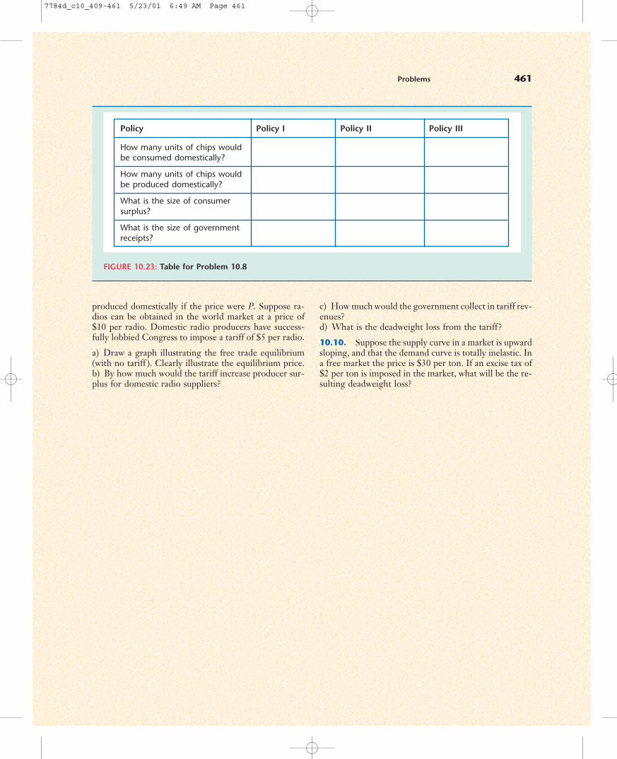
Problems 461
produced domestically if the price were P. Suppose ra-dios can be obtained in the world market at a price of$10 per radio. Domestic radio producers have success-fully lobbied Congress to impose a tariff of $5 per radio.
a) Draw a graph illustrating the free trade equilibrium(with no tariff ). Clearly illustrate the equilibrium price.b) By how much would the tariff increase producer sur-plus for domestic radio suppliers?
c) How much would the government collect in tariff rev-enues?d) What is the deadweight loss from the tariff?
10.10. Suppose the supply curve in a market is upwardsloping, and that the demand curve is totally inelastic. Ina free market the price is $30 per ton. If an excise tax of$2 per ton is imposed in the market, what will be the re-sulting deadweight loss?
FIGURE 10.23: Table for Problem 10.8
Policy Policy I Policy II Policy III
How many units of chips wouldbe consumed domestically?
How many units of chips wouldbe produced domestically?
What is the size of consumersurplus?
What is the size of governmentreceipts?
7784d_c10_409-461 5/23/01 6:49 AM Page 461