competing auctions with endogenous quantities · competing auctions with endogenous quantities...
TRANSCRIPT
Competing Auctions with Endogenous Quantities
Benny Moldovanu, Aner Sela, Xianwen Shi�
December 6, 2006
Abstract
We study models where two sellers simultaneously decide on their discrete supply of a homoge-
nous good. There is a �nite, not necessarily large, number of buyers who have unit demand and
privately known valuations. In the �rst model, there is a centralized market place where a uniform
auction takes place. In the second model, there are two distinct auction sites, each with one seller,
and buyers decide where to bid. Our results shed some light on the conditions leading to either the
emergence of dominant marketplaces or to the coexistence of several competing sites. Using the
theory of potential games, we show that in the one auction site model there is always an (almost
symmetric) equilibrium in pure strategies. This equilibrium approximates the Cournot outcome
as the number of buyers becomes large. In contrast, if the distribution of buyers values has an
increasing failure rate, and if the marginal cost of production is relatively low, there is no pure
strategy equilibrium where both sellers make positive pro�ts in the competing sites model. We also
identify conditions under which an equilibrium with a unique active site exists. Technically, we
are able to deal with the �nite and discrete models by using several results about order statistics
developed by Richard Barlow and Frank Proschan (1965, 1966, 1975).
�Moldovanu: Department of Economics, University of Bonn, Lennestr. 37, 53113 Bonn, Germany; e-mail: mold@uni-
bonn.de. Sela: Department of Economics, Ben Gurion University, Beer Sheva 84105, Israel; e-mail: [email protected].
Shi: Department of Economics, Yale University, 28 Hillhouse Avenue, New Haven, CT 06520, USA; e-mail: xian-
1
1 Introduction
We study models where two sellers simultaneously decide on their (discrete) supply of a homogenous
good, and where there is a �nite, not necessarily large, number of buyers who have unit demand and
privately known valuations.1 In the �rst model, the sellers bring their supply to a centralized market
place where a uniform auction takes place. Thus, by the intrinsic rules of the mechanism, all sold units
command the same price. In the second model, there are two distinct auction sites, each with one seller.
Before observing their value, but after observing the respective supplied quantities at each site, buyers
decide which auction to attend (again, each auction is a uniform price one). In principle, each auction
may have its own equilibrium price.
Our results shed some light on the conditions leading to either the emergence of one dominant
marketplace or the coexistence of several competing sites. In the one auction site model there is always
an (almost symmetric) equilibrium in pure strategies. This equilibrium approximates the Cournot
outcome as the number of buyers becomes large. In contrast, if the distribution of buyers values has
an increasing failure rate (a condition assumed in most of the literature, which implies that marginal
revenue is decreasing), and if the marginal cost of production is relatively low, there is no pure strategy
equilibrium where both sellers make positive pro�ts in the competing sites model. In other words,
two distinct auction sites cannot coexist in equilibrium under these conditions. Coexistence becomes
possible only if the marginal cost of production is su¢ ciently high. We also identify conditions under
which an equilibrium with a unique active site exists.
Another goal of this paper is to revisit several classical scenarios in monopoly and oligopoly theory.
These theories discard the standard assumption of competitive analysis concerning the large number
of producing �rms (sellers), but they keep the assumption that the number of consumers (buyers) is
large. Our model has both a small number of sellers with endogenous supply, and a small number of
buyers.2 This framework is appealing in many situations, in particular in markets for inputs where both
upstream and downstream markets are relatively concentrated oligopolies. Technically, we are able to
deal with the �nite and discrete models by using several results about order statistics developed by
Richard Barlow and Frank Proschan (1965, 1966, 1975).3
One way to unify the two main models of the paper is in terms of buyers�switching cost. If the
switching cost is high, that is, once buyers decide to place a bid in one auction they cannot switch to
the other, we obtain the model with two competing auction sites. If the switching cost is low, then an
ascending clock auction a la Demange-Gale-Sotomayor (this is a variant with money on Gale-Shapley�s
1Most qualitative results can be generalized to settings with more sellers.2The parallels between a single-good auction theory and monopoly are well-known - see Bulow and Roberts (1989).
Hansen (1988) studies a model where sellers compete for the right to become the sole supplier to a unique buyer whose
purchase depends on the winning bid.3For other applications of Barlow and Proschan�s results see Moldovanu, Sela and Shi (2005) and Hoppe, Moldovanu
and Sela (2006).
2
deferred acceptance algorithm) where buyers shift demand to the cheaper unit, leads to an e¢ cient
outcome (conditional on supplied quantities). This outcome is equivalent to the one of the uniform
price auction in the single site model - in particular, all units are sold at a single market price.
Viewed in this perspective, the competing auctions model is one where, in the �rst (quantity-setting)
stage, the sellers compete for market share, i.e., for the buyers that will become locked-in at the second
stage (see Klemperer, 1987 for an early analysis of the forces at play in such models). By increasing
quantity, a seller attracts more buyers.
�Lock-ins�appear in many settings and have a variety of reasons such as transaction costs associ-
ated with operating via several technologically di¤erent platforms/clearing houses, uncertainty about
the quality/quantity o¤ered at other marketplaces, �loyalty�contracts with operators, ex-ante market
speci�c investments, and various forms of network externalities.
On the other hand, a model with a centralized auction site and with endogenous supply is better
suited for the study of some modern markets where all transactions are executed at market price, i.e.,
order driven periodic auctions in �nancial markets, or markets for inputs such as electricity or gas.4 At
online auction sites such as eBay there are often several simultaneous auctions for identical commodities
(e.g., CPU�s). Sajid et al. (2004) empirically study such parallel auctions and �nd that a signi�cant
proportion of bidders are indeed active across the competing auctions: they repeatedly place bids in
the auctions with the lowest standing bid. Moreover, prices tended to be uniform across auctions.
In contrast to our paper, most of the papers in the relatively thin literature on competing auctions
consider models with several sellers endowed with a single unit of a homogenous good, and with several
buyers with unit demand who decide which auction to attend. Thus, total demand and supply are
�xed exogenously, whereas total supply is endogenous in our models. Moreover, most of these papers
use some kind of �large market assumption� for their main results (i.e., individual agents ignore the
e¤ect of their own actions on prices) while such an assumption is not needed here. It is not always clear
whether such assumptions are consistent with a limit obtained in small markets of increased size.
Peters and Severinov (2006) consider several sellers who set reserve prices at their own auctions
sites and then conduct second price auctions. A large number of buyers with unit demand can move
among auction sites. The main consequence of this freedom (i.e., absence of switching costs) is that
there exists an e¢ cient equilibrium (conditional on reserve prices). This is consistent with the insight
obtained from the models that mimic features of the Gale-Shapley deferred acceptance algorithm (such
as our model of competing sellers at a unique auction site) and should be contrasted with earlier models
such as McAfee (1993)5 or Peters and Severinov (1997) where buyers can place only one bid, thus
4Lengwiler (1999), Back and Zender( 2001) and McAdams (2006) analyze endogenous supply in monopolistic models
where the seller adjusts supply after seeing the realization of demand, and where bidders demand several units. LiCalzi
and Pavan (2006) allow the monopolist to ex-ante commit to a supply function. This is in the spirit of Klemperer and
Meyer (1989) who study supply-function equilibria in oligopoly with demand uncertainty.5He considers several sellers o¤ering auctions at �xed sites (each seller at another site). His analysis assumes that the
3
leading to an ine¢ ciency stemming from the coordination problem.
The role of a unique marketplace is also the theme of Moreno and Ubeda (2006) who introduce
an explicit element of price formation in the traditional Cournot oligopoly story (while keeping the
assumption that there is a large number of buyers). Their starting point is the classical paper by
Kreps and Scheinkman (1983) who study a two stage game, with capacity choice in the �rst stage, and
Bertrand competition in the second stage. Kreps and Scheinkman show that the unique equilibrium
coincides with the Cournot outcome. Moreno and Ubeda (2006) look at the two stage model where
�rms �rst choose capacity and then set reservation prices at which they are willing to sell their entire
capacity. The ensuing supply function is used to clear the market. The main di¤erence to the Kreps
and Scheinkman analysis is that all supply is sold at market price whereas, in Kreps and Scheinkman�s
model each �rm charges its own price. This allows them to avoid several di¢ culties appearing in the
Kreps-Scheinkman model.6
If we introduce reserve prices in our model of competing sellers at one auction site, and if we let the
number of buyers go to in�nity (which is the standard assumption in the literature) it can be shown
that, if quantity is optimally adjusted to the number of buyers, the marginal gain from a reserve price
goes to zero.7 The limit outcome is then the classical Cournot one - corresponding to the main result
of Moreno and Ubeda (2006).
An interesting strand that allows for both a small number of buyers and a small number of sellers
is the literature on the so-called strategic market games, following the pioneering work by Shapley and
Shubik (1975). In these models both buyers and sellers bid quantities, and transactions are cleared
at a price equal to the ratio of demand to supply (thus, commodities are allocated in proportion to
bids). Almost the entire literature identi�es the number of trading sites (or �posts�) with the number
of traded commodities. In other words, there is a unique trading site for each traded commodity where
all demand and supply of that commodity is cleared. A notable exception is Koutsougeras (2003) who
allows for two separate trading sites for the same good. In his model traders can send quantity bids
to either one, or to both sites. He shows via an example that the �Law of One Price�need not hold
in equilibrium. Although di¤erent trading prices open up arbitrage opportunities for agents who can
shift their demand/supply (which seems inconsistent with the equilibrium idea), these opportunities
economy is large, and therefore it ignores the e¤ects of individual buyers on prices. In particular, it ignores the fact that
a change in one seller�s mechanism a¤ects the distribution of buyers at his own and at other sites.6The K-S result critically depends on a particular rationing rule used when capacity is binding. Davidson and Deneckere
(1986) show that the Cournot outcome cannot be the equilibrium of the two stage game for any other rationing rule.
Moreover, for a wide range of capacity choices, the equilibrium at the price competition stage is in mixed strategies,
leading to ex-post regret.7This result is based on an analogous observation for a monopolistic �rm that optimally adjusts quantity in response to
a varying number of buyers. Since an increase (decrease) in quantity causes a decrease (increase) in price, a binding reserve
price becomes super�uous as an instrument to control price. This should be contrasted to what happens if competing
sellers have only one unit to sell (Burguet and Sakovics, 1999)
4
disappear when individual agents (who have, relatively speaking, a �large� impact if the number of
traders is small) try to take advantage of them. Such phenomena, which also appear in our model,
nicely illustrate the caution that needs to be employed when dealing with models with a small number
of traders. In particular, market structure may matter a lot: in our model, even mere equilibrium
existence is a¤ected by it.
Our model of competing auction sites with two possibly distinct prices is related to that of Ellison,
Fudenberg and Mobius (2004). These authors study a situation where both sellers and buyers (each
with unit demand/supply) simultaneously choose one of two auction sites.8 Thus, both buyers and
sellers are locked-in at their respective sites, and both total supply and demand in the market are �xed.
Prices are determined by uniform-price auctions at each site (and thus by the ratio of buyers to sellers
at each location).9 Their elegant analysis ignores the integer constraints, and some results hold only for
markets with large numbers of traders.10 Ellison et al. focus on the conditions leading to the existence
of equilibria where two auction sites of unequal size can coexist. Their solved examples involve the
uniform and exponential distributions of values � thus both display an increasing failure rate. Their
coexistence results should be contrasted to ours under this assumption. The di¤erence is mainly due
to the endogenous supply feature in our model.
In a di¤erent vein, Neeman and Vulkan (2001) study the coexistence of two forms of trade: direct
bilateral negotiations and centralized markets.11 In their model, buyers with a high willingness to pay
and sellers with low costs prefer to trade through a centralized market. This leads to an unraveling of
direct negotiations, so that ultimately, all traders opt for trading through the centralized market. Their
analysis uses a reduced form formulation and depends on the assumption that there are large numbers
of traders.
The present paper is organized as follows. In Section 2 we describe the basic model ingredients
and introduce useful de�nitions and notation. In Section 3 we study the case of one auction site. In
Subsection 3.1 we start with a monopolistic seller using a uniform price auction. We focus on the optimal
supplied quantity, and we show that it increases in the convexity of the distribution function of buyers�
valuations. This allows us to derive optimal quantity estimates for large, non-parametric families of
distributions (i.e., with monotone hazard rates, concave, convex) . In subsection 3.2 we remain in the
single auction-site model, but add competition among sellers: each of two ex-ante symmetric sellers
provides the auctioneer with several units of a homogenous good, and the auctioneer sells the total
quantity via a uniform price auction. With a large number of buyers, this is equivalent to classical
Cournot competition. Using the potential game approach (due to Monderer and Shapley, 1996) we
8This is an application of a more general framework developed by Ellison and Fudenberg (2002)9We could have also presented our model by assuming that: 1) every unit is owned by a di¤erent seller; 2) the operator
of each auction site restricts entry of sellers in order to maximize total pro�t at the site.10Anderson et al. (2005) retake this analysis while incorporating the integer constraints since ignoring them may lead
to inconsistent results.11Genesove (1995) o¤ers an insightful study of such an arrangement in the New England �sh industry.
5
prove the existence of pure-strategy Nash equilibria for any constant marginal cost. Moreover, we show
that an �almost� symmetric equilibrium, where the supplied quantities di¤er by at most one unit,
always exists. Finally, we use the above described estimates in the monopoly case to give estimates for
the total quantity under competition. In Subsection 3.3 we o¤er an example illustrating that a merger
of auction sites may not be pro�table if sellers optimize supply before and after a merger (although
a merger is always e¢ ciency increasing). This contrasts an earlier insight due to Schwartz and Ungo
(2002) who considered sellers with exogenously given quantities.
In Section 4 we turn to the model with two distinct auction sites, each with one seller: First, the
two sellers simultaneously choose the number of units supplied in their respective auctions. Before
they learn their valuations, but after they observe the sellers�decisions, buyers choose which auction
to attend. In the last stage, each buyer learns his valuation and submits a bid in his selected auction.
In Subsection 4.1 we study the possibility of coexistence of two auction sites. A main result is that if
the marginal production cost is low enough, and if the distribution of buyers�values has an increasing
hazard rate then there is no pure strategy equilibrium in which both sellers are active and make positive
pro�ts. The reason is that each seller continually increases supply in order to snatch buyers from the
other site. A coexistence equilibrium is possible only if the marginal cost of production is high enough.
Then, the unilateral incentives to increase supply are capped by the production cost. In Subsection 4.2
we study equilibria where only one auction site is active (i.e., the other seller prefers to stay out). Such
an equilibrium is possible if the optimal monopolistic quantity produced by the active seller is high
enough to deter entry � this happens, for example, if the distribution of buyers�values is su¢ ciently
convex, and if the marginal cost is not too high.
In Section 5 we compare the equilibrium quantities and prices across three di¤erent models (monopoly,
competition at one auction site, and two competing auction sites) under the assumption that there is
a large number of buyers. We show that, under a mild condition, the monopoly model has the highest
price and lowest quantity in equilibrium. Furthermore, if the equilibrium supply is relatively high (e.g.,
if the production cost is low and the distribution of buyers�valuations is su¢ ciently convex), the model
with two auction sites is more competitive than the model with one auction site: the equilibrium price
is lower and the equilibrium quantity is higher in the former model. Finally, if the equilibrium supply
is relatively low, then the reverse is true.
Section 6 contains several concluding comments. Appendix A contains several useful results from
the literature on order statistics. Appendix B contains all proofs.
6
2 The Model
There are two competing sellers and n � 2 buyers. The sellers can each produce several units of a
homogenous good. Each buyer has unit demand. The valuation of buyer j for a unit of the good is
private information to j: Valuations are drawn independently of each other from the interval [0; T ] ; T �
1; according to a distribution function F that is common knowledge.
We consider two di¤erent competition models among the sellers:
1. One auction site: Sellers 1 and 2 simultaneously provide k1 and k2 units to the auctioneer,
respectively. Then the auctioneer sells the (k1 + k2) units via a uniform price auction. The revenue of
each seller is the product of the equilibrium price and his supplied quantity.
2. Two competing auction sites: In the �rst stage, sellers 1 and 2 simultaneously choose the
number of objects for sale ki, i = 1; 2; in their own auctions. In the second stage, before they learn
their valuations, but after they know the decision made by the sellers in the �rst stage, buyers choose
whether to attend auction 1 or 2. In the third and last stage, each buyer learns his valuation and
submits a bid in his selected auction (each of the two auctions is a uniform price auction). The revenue
of each seller is the product of his supplied quantity and equilibrium price in his own auction.
2.1 Notation
We use the following notation: Xk;n denotes k-th order statistic out of n independent valuations dis-
tributed according to F (note that Xn;n is the highest order statistic, and so on..). The distribution
Fk;n and the density fk;n of Xk;n are given by
Fk;n(x) =
nXj=k
�n
j
�F (x)j [1� F (x)]n�j
fk;n(x) =n!
(k � 1)!(n� k)!F (x)k�1[1� F (x)]n�kf(x)
We denote by EXk;n the expected value of Xk;n.
The failure rate (or hazard rate) of a distribution F is de�ned by:
� (x) =f (x)
1� F (x)
A distribution function F has an increasing failure rate (IFR) if its failure (or hazard) rate, � (x) ;
is increasing. Analogously, F has an decreasing failure rate (DFR) if � (x) is decreasing. Note that
convexity of F implies IFR , while DFR implies concavity. The only distribution that is both concave
and convex is the uniform, while the only distribution that is both IFR and DFR is the exponential.
A distribution function F is star-shaped on [0; T ] if F (x)=x is increasing in x. Let X(Z) have
distributions F (G) such that F (0) = G(0) = 0: Distribution F is star-shaped with respect to G if the
function G�1F (x) is star-shaped. Notice that :
7
1. If F (0) = 0 = G (0) ; G�1F convex implies G�1F star-shaped.
2. If G is the exponential distribution, then G�1F convex is equivalent to F being IFR.
3. If G is uniform, then G�1F convex is equivalent to F is convex.
3 One Auction Site
We discuss �rst the model of a uniform price multi-object auction with n buyers and a single, monopolist
seller with variable supply. The derived insights will be repeatedly used in the analysis of competition
among sellers below.
3.1 Monopoly seller
The seller decides on the supply k , and then the buyers decide what to bid in an uniform price auction
for k units. We do not explicitly analyze here the use of exclusion tools such as reserve prices and entry
fees. Thus all n buyers have an incentive to participate in the auction. Note that in an auction with
endogenous quantity and large number of buyers, the marginal gain from setting optimal reserve price
is small if quantity is optimally set. The intuition is provided by the fact that the realizations of Xn�k:n
are very close to EXn�k;n if n is large. The seller can control EXn�k;n by varying the quantity k: If
the reserve price is binding and enhancing revenue, the seller can always set the quantity to k0 such
that, approximately, EXn�k0;n = r: After this adjustment, the reserve price is redundant.
We assume �rst that the seller has a zero cost of producing the object. If the seller o¤ers k > n
objects, it is obvious that the equilibrium price is zero, and the seller has zero pro�t. Thus, without
loss of generality, we restrict attention to the case k � n: In the auction, each of the k highest buyers
wins a single unit, and pays the equilibrium price Xn�k;n. In expectation, the seller�s maximization
problem is given by
maxkR (k; n) = max
kkEXn�k;n
The relation between the optimal number of objects and the distribution of the buyers�valuation is
as follows:
Proposition 1 Consider two distributions G;F leading to optimal supplies k�G(n) and k�F (n) , respec-
tively, when there are n buyers. If G�1F is star-shaped then k�G(n) � k�F (n):
Proposition 1 implies the following two corollaries:
Corollary 1 If F is IFR (DFR), and n is large, then k�F (n); the optimal supply in an auction with n
buyers satis�es k�F (n) � (�) ne ; where e is the natural logarithm basis.
8

Corollary 2 If F is convex(concave), then k�F (n); the optimal supply in the auction with n buyers
satis�es k�F (n) � (�) n2 :
The following result considers the function k�F (n) that relates the optimal supply to the number of
buyers. It shows that the �slope�of this function is less than unity if F is IFR (thus, the di¤erence
n� k�(n) weakly increases in n)
Proposition 2 Let k�F (n) be the optimal number of objects in the auction with n buyers. If F is IFR,
then, for all n; k�F (n+ 1)� k�F (n) � 1:
Remark 1 When n is large we have the approximation
EXn�k;n � F�1�n� kn
�Hence, the seller�s revenue in our auction is
R1 (k; n) = kEXn�k;n � kF�1�n� kn
�= kF�1
�1� k
n
�Consider now a monopolist seller facing n buyers, each with unit demand and valuation distribution F:
The monopolist chooses p to maximize his expected revenue.
R2 (p; n) = np [1� F (p)]
Setting k = n [1� F (p)] ; or equivalently p = F�1�1� k
n
�; we see that the monopoly and auction models
are equivalent if the number of buyers is su¢ ciently large. In particular, p�; the limit equilibrium price
in a single auction with endogenous quantity and a su¢ ciently large number of buyers is given by
�(p�) =f (p�)
1� F (p�) =1
p�
Note that an increase of the distribution of the buyers�valuations in the hazard rate order (which implies
�rst-order stochastic dominance) yields a higher equilibrium price.
Example 1 Let F (x) = x1=a (a > 0) with support [0; 1] : When n is large, the seller�s revenue if he
sells k objects is
R (k; n; a) = kEXn�k;n � kF�1�n� kn
�= k
�n� kn
�aThe optimal k is
k�F (n) =1
a+ 1n
and we have k�F (n; a)� < n=2 if a > 1 and k�F (n; a) > n=2 if a < 1: The limit equilibrium price is
p�(a) = ( aa+1 )
a:
9
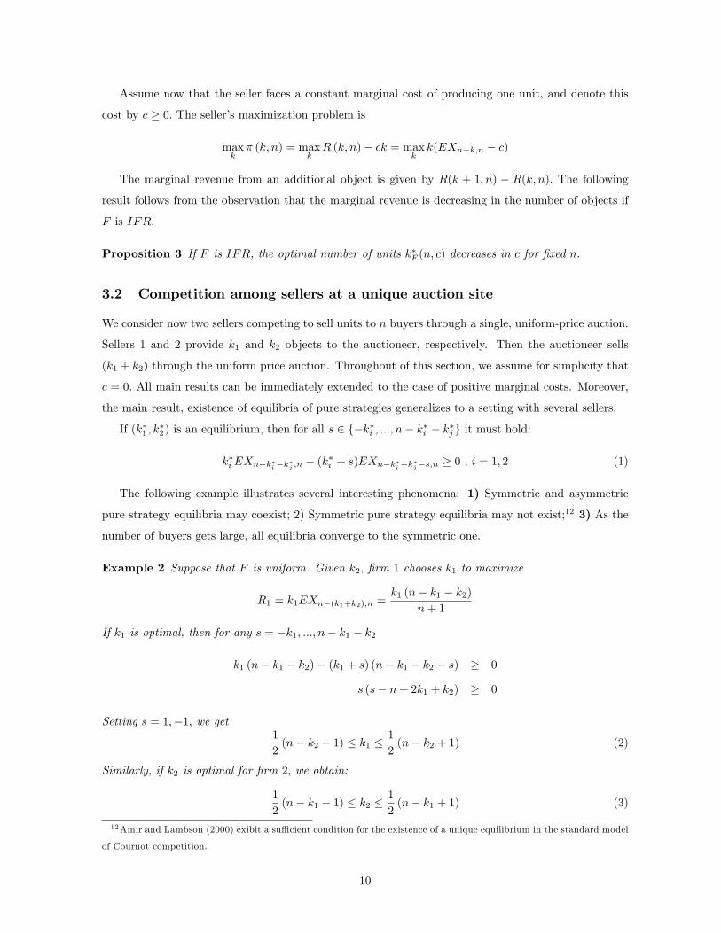
Assume now that the seller faces a constant marginal cost of producing one unit, and denote this
cost by c � 0: The seller�s maximization problem is
maxk� (k; n) = max
kR (k; n)� ck = max
kk(EXn�k;n � c)
The marginal revenue from an additional object is given by R(k + 1; n) � R(k; n): The following
result follows from the observation that the marginal revenue is decreasing in the number of objects if
F is IFR.
Proposition 3 If F is IFR, the optimal number of units k�F (n; c) decreases in c for �xed n:
3.2 Competition among sellers at a unique auction site
We consider now two sellers competing to sell units to n buyers through a single, uniform-price auction.
Sellers 1 and 2 provide k1 and k2 objects to the auctioneer, respectively. Then the auctioneer sells
(k1 + k2) through the uniform price auction. Throughout of this section, we assume for simplicity that
c = 0: All main results can be immediately extended to the case of positive marginal costs. Moreover,
the main result, existence of equilibria of pure strategies generalizes to a setting with several sellers.
If (k�1 ; k�2) is an equilibrium, then for all s 2 f�k�i ; :::; n� k�i � k�j g it must hold:
k�iEXn�k�i�k�j ;n � (k�i + s)EXn�k�i�k�j�s;n � 0 , i = 1; 2 (1)
The following example illustrates several interesting phenomena: 1) Symmetric and asymmetric
pure strategy equilibria may coexist; 2) Symmetric pure strategy equilibria may not exist;12 3) As the
number of buyers gets large, all equilibria converge to the symmetric one.
Example 2 Suppose that F is uniform. Given k2; �rm 1 chooses k1 to maximize
R1 = k1EXn�(k1+k2);n =k1 (n� k1 � k2)
n+ 1
If k1 is optimal, then for any s = �k1; :::; n� k1 � k2
k1 (n� k1 � k2)� (k1 + s) (n� k1 � k2 � s) � 0
s (s� n+ 2k1 + k2) � 0
Setting s = 1;�1; we get1
2(n� k2 � 1) � k1 �
1
2(n� k2 + 1) (2)
Similarly, if k2 is optimal for �rm 2; we obtain:
1
2(n� k1 � 1) � k2 �
1
2(n� k1 + 1) (3)
12Amir and Lambson (2000) exibit a su¢ cient condition for the existence of a unique equilibrium in the standard model
of Cournot competition.
10
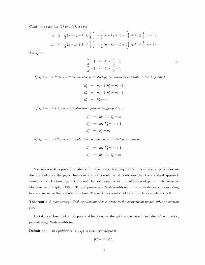
Combining equation (2) and (3), we get
k1 � 1
2(n� k2 � 1) �
1
2
�n� 1
2(n� k1 + 1)� 1
�) k1 �
1
3(n� 3)
k1 � 1
2(n� k2 + 1) �
1
2
�n� 1
2(n� k1 � 1) + 1
�) k1 �
1
3(n+ 3)
Therefore,
n
3� 1 � k1 �
n
3+ 1 (4)
n
3� 1 � k2 �
n
3+ 1
1) If n = 3m there are three possible pure strategy equilibria (see details in the Appendix)
k�1 = m+ 1; k�2 = m� 1
k�1 = m� 1; k�2 = m+ 1
k�1 = k�2 = m
2) If n = 3m+ 1; there are also three pure-strategy equilibria
k�1 = m+ 1; k�2 = m
k�1 = m; k�2 = m+ 1
k�1 = k�2 = m
3) If n = 3m+ 2; there are only two asymmetric pure strategy equilibria
k�1 = m; k�2 = m+ 1
k�1 = m+ 1; k�2 = m
We turn now to a proof of existence of pure-strategy Nash equilibria. Since the strategy spaces are
discrete and since the payo¤ functions are not continuous, it is obvious that the standard approach
cannot work. Fortunately, it turns out that our game is an ordinal potential game in the sense of
Monderer and Shapley (1996). Thus it possesses a Nash equilibrium in pure strategies, corresponding
to a maximizer of the potential function. The next two results hold also for the case where c > 0.
Theorem 1 A pure strategy Nash equilibrium always exists in the competition model with one auction
site.
By taking a closer look at the potential function, we also get the existence of an �almost�symmetric,
pure-strategy Nash equilibrium:
De�nition 1 An equilibrium (k�1 ; k�2) is quasi-symmetric if
jk�1 � k�2 j � 1:
11
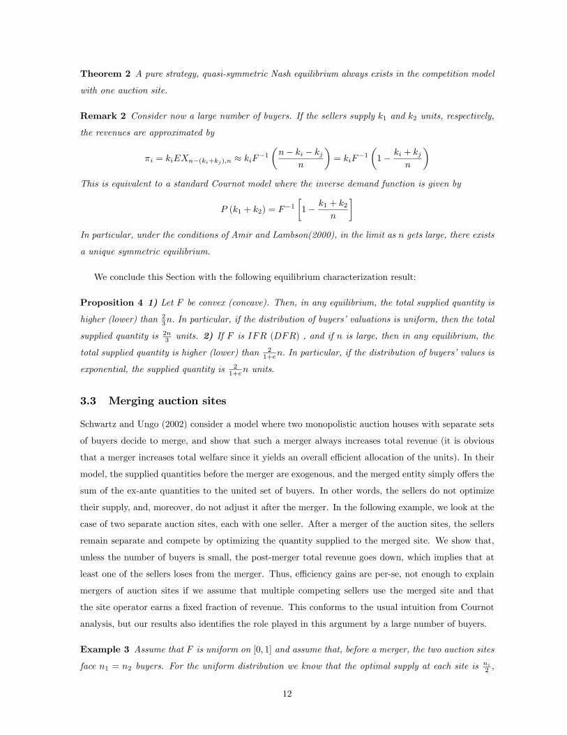
Theorem 2 A pure strategy, quasi-symmetric Nash equilibrium always exists in the competition model
with one auction site.
Remark 2 Consider now a large number of buyers. If the sellers supply k1 and k2 units, respectively,
the revenues are approximated by
�i = kiEXn�(ki+kj);n � kiF�1�n� ki � kj
n
�= kiF
�1�1� ki + kj
n
�This is equivalent to a standard Cournot model where the inverse demand function is given by
P (k1 + k2) = F�1�1� k1 + k2
n
�In particular, under the conditions of Amir and Lambson(2000), in the limit as n gets large, there exists
a unique symmetric equilibrium.
We conclude this Section with the following equilibrium characterization result:
Proposition 4 1) Let F be convex (concave). Then, in any equilibrium, the total supplied quantity is
higher (lower) than 23n: In particular, if the distribution of buyers�valuations is uniform, then the total
supplied quantity is 2n3 units. 2) If F is IFR (DFR) , and if n is large, then in any equilibrium, the
total supplied quantity is higher (lower) than 21+en: In particular, if the distribution of buyers�values is
exponential, the supplied quantity is 21+en units.
3.3 Merging auction sites
Schwartz and Ungo (2002) consider a model where two monopolistic auction houses with separate sets
of buyers decide to merge, and show that such a merger always increases total revenue (it is obvious
that a merger increases total welfare since it yields an overall e¢ cient allocation of the units). In their
model, the supplied quantities before the merger are exogenous, and the merged entity simply o¤ers the
sum of the ex-ante quantities to the united set of buyers. In other words, the sellers do not optimize
their supply, and, moreover, do not adjust it after the merger. In the following example, we look at the
case of two separate auction sites, each with one seller. After a merger of the auction sites, the sellers
remain separate and compete by optimizing the quantity supplied to the merged site. We show that,
unless the number of buyers is small, the post-merger total revenue goes down, which implies that at
least one of the sellers loses from the merger. Thus, e¢ ciency gains are per-se, not enough to explain
mergers of auction sites if we assume that multiple competing sellers use the merged site and that
the site operator earns a �xed fraction of revenue. This conforms to the usual intuition from Cournot
analysis, but our results also identi�es the role played in this argument by a large number of buyers.
Example 3 Assume that F is uniform on [0; 1] and assume that, before a merger, the two auction sites
face n1 = n2 buyers. For the uniform distribution we know that the optimal supply at each site is ni2 ;
12
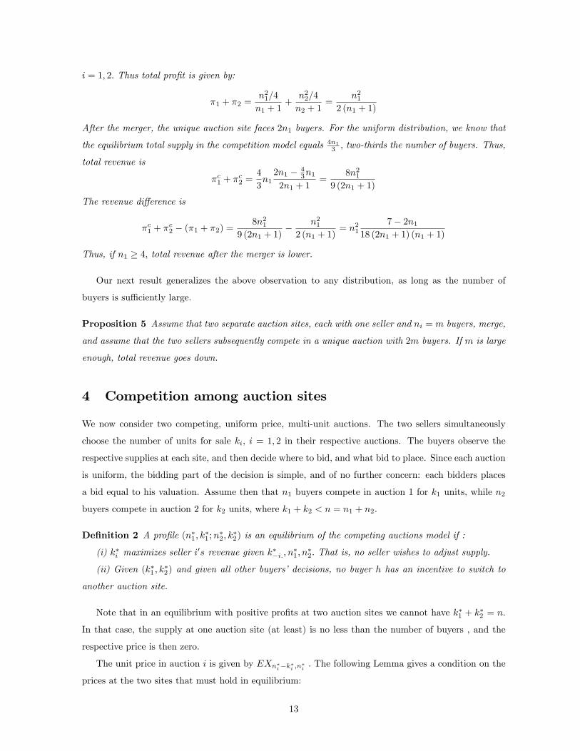
i = 1; 2: Thus total pro�t is given by:
�1 + �2 =n21=4
n1 + 1+n22=4
n2 + 1=
n212 (n1 + 1)
After the merger, the unique auction site faces 2n1 buyers. For the uniform distribution, we know that
the equilibrium total supply in the competition model equals 4n13 ; two-thirds the number of buyers. Thus,
total revenue is
�c1 + �c2 =
4
3n12n1 � 4
3n1
2n1 + 1=
8n219 (2n1 + 1)
The revenue di¤erence is
�c1 + �c2 � (�1 + �2) =
8n219 (2n1 + 1)
� n212 (n1 + 1)
= n217� 2n1
18 (2n1 + 1) (n1 + 1)
Thus, if n1 � 4; total revenue after the merger is lower.
Our next result generalizes the above observation to any distribution, as long as the number of
buyers is su¢ ciently large.
Proposition 5 Assume that two separate auction sites, each with one seller and ni = m buyers, merge,
and assume that the two sellers subsequently compete in a unique auction with 2m buyers. If m is large
enough, total revenue goes down.
4 Competition among auction sites
We now consider two competing, uniform price, multi-unit auctions. The two sellers simultaneously
choose the number of units for sale ki, i = 1; 2 in their respective auctions. The buyers observe the
respective supplies at each site, and then decide where to bid, and what bid to place. Since each auction
is uniform, the bidding part of the decision is simple, and of no further concern: each bidders places
a bid equal to his valuation. Assume then that n1 buyers compete in auction 1 for k1 units, while n2
buyers compete in auction 2 for k2 units, where k1 + k2 < n = n1 + n2:
De�nition 2 A pro�le (n�1; k�1 ;n
�2; k
�2) is an equilibrium of the competing auctions model if :
(i) k�i maximizes seller i0s revenue given k��i:; n
�1; n
�2: That is, no seller wishes to adjust supply.
(ii) Given (k�1 ; k�2) and given all other buyers� decisions, no buyer h has an incentive to switch to
another auction site.
Note that in an equilibrium with positive pro�ts at two auction sites we cannot have k�1 + k�2 = n:
In that case, the supply at one auction site (at least) is no less than the number of buyers , and the
respective price is then zero.
The unit price in auction i is given by EXn�i�k�i ;n�i : The following Lemma gives a condition on the
prices at the two sites that must hold in equilibrium:
13
Lemma 1 Consider any �xed strategy pro�le for the two sellers and for all buyers except h. Then,
it is optimal for h to join the auction with the lower expected price. Moreover, in any equilibrium,
(n�1; k�1 ;n
�2; k
�2) it must hold that
EXn�i�k�i ;n�i � EXn�j�k�j ;n�j ) EXn�i�k�i ;n�i � EXn�j+1�k�j ;n�j+1
In other words, in equilibrium, it cannot be pro�table for a buyer in the auction with a higher
expected price to move to the other auction. Thus, while equilibrium prices at the two auction sites
need not be strictly equal, there are no arbitrage opportunities.
4.1 Equilibrium coexistence of two auction sites
Our main result in this section is that two auction sites yielding positive pro�ts for the respective sellers
cannot coexist in equilibrium if the distribution of buyers�values is IFR; and if the marginal production
cost, c; is su¢ ciently low. The proof is based on the following Lemma which has some independent
interest. It shows that, for any pro�le of buyers�actions, at least one of the sellers has an incentive to
increase supply if F is IFR:
Lemma 2 1. Consider any con�guration (n1; k1;n2; k2) where n1; n2 > 0; k1; k2 > 0 and k1+k2 < n;
and assume that buyers play a best response to any announcement of quantities. If EXni�ki;ni �
EXnj�kj ;nj ; i; j = 1; 2; then seller i can attract at least one more buyer by supplying one additional
unit.
2. Assume that F is IFR; and that c = 0: For any con�guration (n1; k1;n2; k2) where n1; n2 > 0;
k1; k2 > 0 and k1 + k2 < n, one of the sellers can increase his pro�t by supplying one additional
unit.
3. If F is IFR; and if c = 0; then �R(k; n) = R(k + 1; n + 1) � R(k; n), the marginal revenue of
seller whose supply increases from k to k + 1 while the number of buyers attending his auction
increases from n to n+ 1, decreases in k for a �xed n:
The Lemma yields:
Theorem 3 Assume that F is IFR: Then, for su¢ ciently small marginal production costs c; there is
no equilibrium in which both sellers are active and make positive pro�ts. In particular, if
c <n
2EX1;n2+1 � (
n
2� 1)EX1;n2 (5)
there is no symmetric equilibrium with positive pro�ts.
If the IFR condition is not satis�ed, or if the cost is high enough (in contrast to the assumptions
of the above Proposition) an equilibrium where two auction sites are active, and where both sellers
14
make positive pro�ts may then exist. We look �rst at an example where F does not satisfy the IFR
condition:
Example 4 Let F (x) = x1=2; and let c = 0: Then:
�R (ki; ni) =(ki + 1)(ni � ki + 1)(ni � ki)
(ni + 2)(ni + 3)� ki(ni � ki + 1)(ni � ki)
(ni + 1)(ni + 2)
=(ni � ki)(ni � ki + 1)(ni + 1� 2ki)
(ni + 1)(ni + 2)(ni + 3)
Note that �R (ki; ni) � 0 if ki � ni+12 : Letting k1 = k2 = 2 and n1 = n2 = 3; it is clear that no seller
has an incentive to increase supply . Assume then that seller 1, say, lowers supply to one unit. Then a
buyer attending his auction has an incentive to switch to the other auction since there the price will be
EX2;4 < EX2;3: Therefore no seller has an incentive to deviate, and we obtain a symmetric equilibrium
in which every seller sells two units and makes a positive pro�t:13
Next we look at situations where the marginal cost c is su¢ ciently high, Then, sellers do not want
to increase their supply above a certain level (since the price drops below cost), and an equilibrium may
exist.
If, in a symmetric equilibrium, a seller sells k� units, he should have no incentive to increase supply
to k� + 1. Then, for F which is IFR; we have the necessary condition14
p = EXn2�k�;
n2> c > (k� + 1)EXn
2�k�;n2+1
� k�EXn2�k�;
n2
(6)
where the left inequality indicates that a seller makes a positive pro�t by selling k� units to half the
number of buyers, and the right inequality indicates that a seller has no incentive to increase the number
of supplied units from k� to k� + 1 if by doing so the number of buyers attending his auction increases
from n2 to
n2 + 1.
The following proposition provides a su¢ cient condition for existence of a symmetric equilibrium
with the maximal supply value for which both sellers make positive pro�ts.
Proposition 6 Assume that F is IFR. If
(n
2� 1)EX(2;n2+1) � (
n
2� 2)EX(2;n2 ) > c >
n
2EX(1;n2+1) � (
n
2� 1)EX(1;n2 ) (7)
then the pro�le where each seller sells n2 � 1 objects to
n2 buyers constitutes a symmetric equilibrium.
4.2 A unique auction site as the outcome of competition
We now focus on equilibria where only one auction site is active, and where only one seller makes a
positive pro�t. Roughly speaking, such an equilibrium may exist if the optimal monopolistic quantity
13 In this example there is also a symmetric equilibrium where each seller supplies three units, and where pro�ts are
zero.14 If F is IFR; by lemma 2 the RHS of (6) is always positive.
15
for the unique active seller is high enough. Then, the other seller cannot convince enough buyers to
switch to his own auction, and thus prefers to stay out.
Formally, an equilibrium with the form (n�1 = n; k�1 > 0; n
�2 = 0; k
�2 = 0) exists if and only if:
1.
k�1 = argmaxkk(EXn�k;n � c) > 0 (8)
and
2. For all k2 � n� k�1 ; either the set M =M(k2) = fm j m � n� k�1 ^ EXm�k2;m � cg is empty or
EXen2�k2;en2 > EXn�en2+1�k�1 ;n�en2+1 (9)
where en2 = en2(k2) is the minimal element in M:Condition (8) requires that seller 1 optimizes his (monopolistic) supply and makes a positive pro�t,
given that seller 2 is not active. In condition (9), en2 is the minimal number of buyers for which sellingk2 units is pro�table for seller 2. Note that if condition (9) holds and if n2 > en2 , we also get
EXn2�k2;n2 > EXen2�k2;en2 > EXn�en2+1�k�1 ;n�en2+1 = EXn�n2+(n2�en2+1)�k�1 ;n�n2+(n2�en2+1)The �rst inequality follows by repeated application of the known relation EX(i+1;n+1) � EX(i;n);
and the second inequality is condition (9). That is, condition (9) guarantees that if n2 > en2 buyersattend auction 2, at least (n2 � en2 + 1) buyers will want to switch to auction 1. Thus, seller 2 mustremain inactive, and earns zero pro�t.
Proposition 7 1. Assume that k�1 = argmaxk k(EXn�k;n � c) is su¢ ciently large (For example,
assume that F is su¢ ciently convex and that c is su¢ ciently small). Then there exists an asymmetric
equilibrium with a unique active seller.
2. Assume that k�1 = argmaxk k(EXn�k;n � c) < n2 : (For example, assume that F is su¢ ciently
concave) Then there exists no equilibrium with a unique active seller.
The following examples illustrates the result.
Example 5 Let c = 0; n = 4 and let F be uniform on [0; 1]. By Corollary 2 the optimal supply for
a monopolistic seller 1 is k�1 = 2. The only alternative for seller 2 that leads to a positive pro�t is to
supply one unit. Since EX1;2 � EX4�1�2;4�1 = EX1;2 � EX1;3 > 0 , condition (9) is satis�ed. Seller
2 cannot attract more than one buyer to his auction, and he therefore prefers to stay out.
16
5 Comparison among models
How do the models analyzed in this paper (and in particular the competition models with either one or
two auctions sites) compare in terms of equilibrium prices and quantities ? In this section we answer
this question under the assumption that the number of buyers is large. We consider the following:
� Monopoly (M): one auction site with one seller and n buyers;
� Competition among sellers at one auction site (C1): two competing sellers at one auction site
with n buyers;
� Competing auctions (C2): two sellers running separate auctions, competing to attract n buyers.
For the results below we assume that a symmetric equilibrium exists in this model.
Proposition 8 Assume that F; the distribution of buyers� values, is IFR. Assume total equilibrium
supply in all three models is at least n3 + 2: (This happens, for example, if either F is convex enough
with respect to the exponential distribution, or if the marginal cost is not too high). Then the following
hold:
(1) The equilibrium price under monopoly is higher than the prices in symmetric equilibria of the
competition models.
(2) If total supply is higher (lower) than n2 + 2; then the equilibrium price in the competition model
with one auction site is higher (lower) than the equilibrium price in the competition model with two
auction sites.
6 Concluding remarks
We have studied competition among two sellers who optimize their respective supply in markets with a
�nite, not necessarily large, number of buyers. We studied a model where all transactions take place at
price determined in one auction, and another where there two separate auction sites may operate side
by side. A uni�ed perspective on both models can be obtained by considering buyers�switching costs.
Whereas an equilibrium where both sellers make pro�ts always exists in the �rst model (one auction
site), this is not the case in the second model (two auction sites) under ubiquitous conditions on the
demand function (decreasing marginal revenue) and on the supply functions (su¢ ciently low marginal
costs). In markets with sinking production (or trading) costs, our results suggest a movement towards
dominant market places featuring several competing suppliers. Ebay is an obvious example. Instead
of a competition mode characterized by poaching business from competitors, we currently observe a
move towards consolidation also in the trading of securities.15 For example, on October 17th 2006 the
Chicago Mercantile Exchange agreed to buy the Chicago Board of Trade, thus aiming to create the
15See "The Big Squeeze", The Economist, October 7th, 2006, pp. 83.
17
world�s biggest �nancial marketplace.16 Similarly, the Deutsche Börse has long argued for the need of a
pan-European exchange, and tried (unsuccessfully) to buy the London Stock Exchange �which is now
on NASDAQ�s buying list.
Finally, we hope that the mathematical methods used in this paper will prove to be useful in a
variety of other competition models with a small number of traders.
7 Appendix A
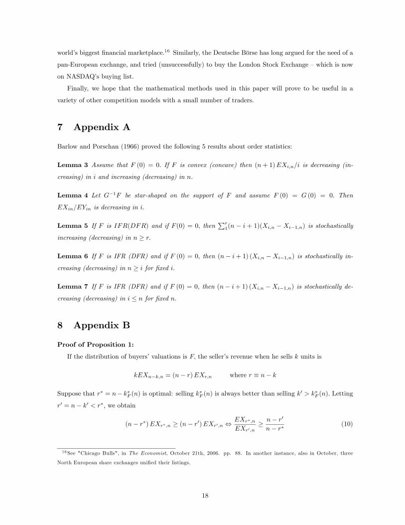
Barlow and Porschan (1966) proved the following 5 results about order statistics:
Lemma 3 Assume that F (0) = 0: If F is convex (concave) then (n+ 1)EXi;n=i is decreasing (in-
creasing) in i and increasing (decreasing) in n.
Lemma 4 Let G�1F be star-shaped on the support of F and assume F (0) = G (0) = 0: Then
EXin=EYin is decreasing in i:
Lemma 5 If F is IFR(DFR) and if F (0) = 0; thenPr
1(n � i + 1)(Xi;n � Xi�1;n) is stochastically
increasing (decreasing) in n � r:
Lemma 6 If F is IFR (DFR) and if F (0) = 0; then (n� i+ 1) (Xi;n �Xi�1;n) is stochastically in-
creasing (decreasing) in n � i for �xed i:
Lemma 7 If F is IFR (DFR) and if F (0) = 0; then (n� i+ 1) (Xi;n �Xi�1;n) is stochastically de-
creasing (decreasing) in i � n for �xed n:
8 Appendix B
Proof of Proposition 1:
If the distribution of buyers�valuations is F; the seller�s revenue when he sells k units is
kEXn�k;n = (n� r)EXr;n where r � n� k
Suppose that r� = n� k�F (n) is optimal: selling k�F (n) is always better than selling k0 > k�F (n): Letting
r0 = n� k0 < r�; we obtain
(n� r�)EXr�;n � (n� r0)EXr0;n ,EXr�;nEXr0;n
� n� r0n� r� (10)
16See "Chicago Bulls", in The Economist, October 21th, 2006. pp. 88. In another instance, also in October, three
North European share exchanges uni�ed their listings.
18
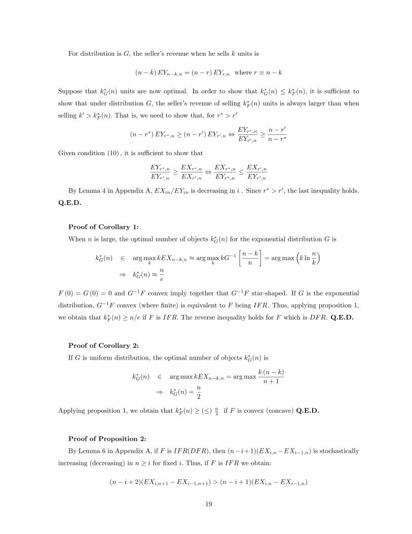
For distribution is G; the seller�s revenue when he sells k units is
(n� k)EYn�k;n = (n� r)EYr;n where r � n� k
Suppose that k�G(n) units are now optimal. In order to show that k�G(n) � k�F (n); it is su¢ cient to
show that under distribution G; the seller�s revenue of selling k�F (n) units is always larger than when
selling k0 > k�F (n): That is, we need to show that, for r� > r0
(n� r�)EYr�;n � (n� r0)EYr0;n ,EYr�;nEYr0;n
� n� r0n� r�
Given condition (10) ; it is su¢ cient to show that
EYr�;nEYr0;n
� EXr�;nEXr0;n
, EXr�;nEYr�;n
� EXr0;nEYr0;n
By Lemma 4 in Appendix A, EXin=EYin is decreasing in i . Since r� > r0; the last inequality holds.
Q.E.D.
Proof of Corollary 1:
When n is large, the optimal number of objects k�G(n) for the exponential distribution G is
k�G(n) 2 argmaxkkEXn�k;n � argmax
kkG�1
�n� kn
�= argmax
�k ln
n
k
�) k�G(n) �
n
e
F (0) = G (0) = 0 and G�1F convex imply together that G�1F star-shaped. If G is the exponential
distribution, G�1F convex (where �nite) is equivalent to F being IFR. Thus, applying proposition 1,
we obtain that k�F (n) � n=e if F is IFR: The reverse inequality holds for F which is DFR. Q.E.D.
Proof of Corollary 2:
If G is uniform distribution, the optimal number of objects k�G(n) is
k�G(n) 2 argmax kEXn�k;n = argmaxk (n� k)n+ 1
) k�G(n) =n
2
Applying proposition 1, we obtain that k�F (n) � (�) n2 if F is convex (concave) Q.E.D.
Proof of Proposition 2:
By Lemma 6 in Appendix A, if F is IFR(DFR); then (n� i+1)(EXi;n�EXi�1;n) is stochastically
increasing (decreasing) in n � i for �xed i: Thus, if F is IFR we obtain:
(n� i+ 2)(EXi;n+1 � EXi�1;n+1) > (n� i+ 1)(EXi;n � EXi�1;n)
19
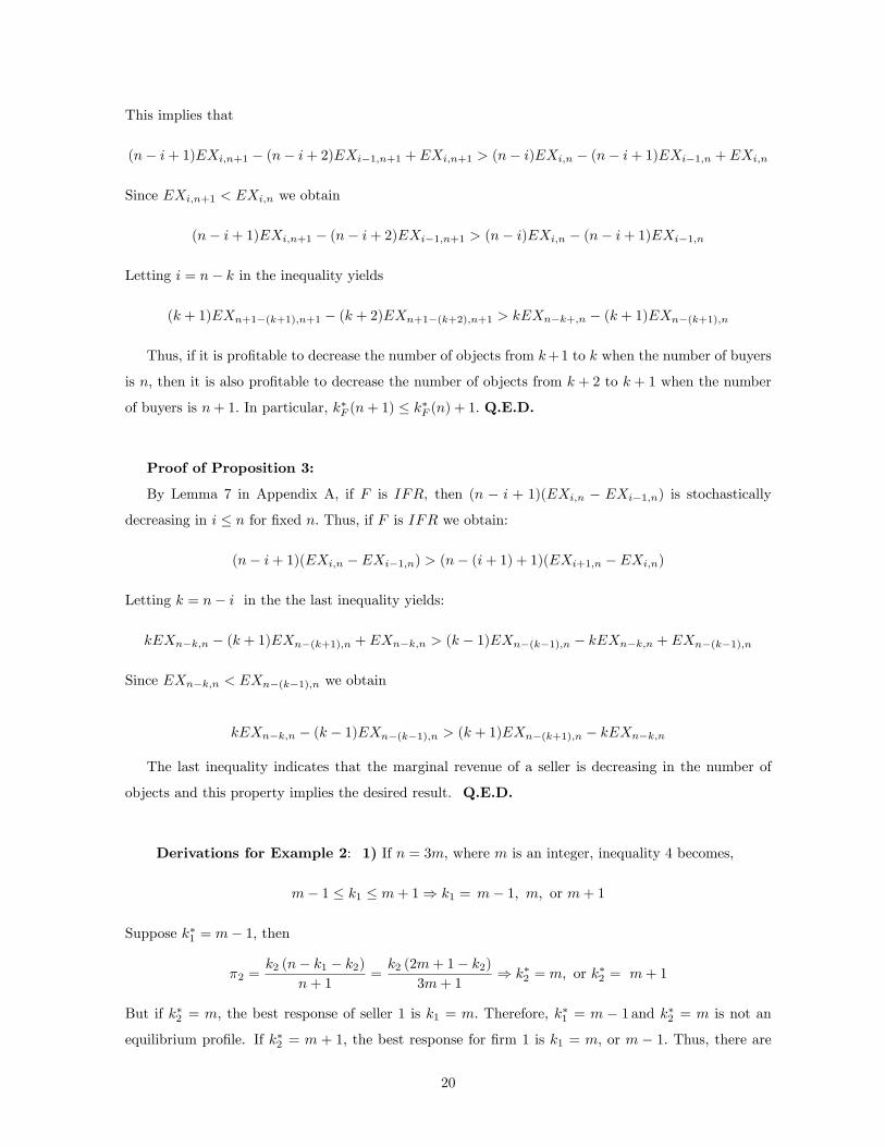
This implies that
(n� i+ 1)EXi;n+1 � (n� i+ 2)EXi�1;n+1 + EXi;n+1 > (n� i)EXi;n � (n� i+ 1)EXi�1;n + EXi;n
Since EXi;n+1 < EXi;n we obtain
(n� i+ 1)EXi;n+1 � (n� i+ 2)EXi�1;n+1 > (n� i)EXi;n � (n� i+ 1)EXi�1;n
Letting i = n� k in the inequality yields
(k + 1)EXn+1�(k+1);n+1 � (k + 2)EXn+1�(k+2);n+1 > kEXn�k+;n � (k + 1)EXn�(k+1);n
Thus, if it is pro�table to decrease the number of objects from k+1 to k when the number of buyers
is n; then it is also pro�table to decrease the number of objects from k + 2 to k + 1 when the number
of buyers is n+ 1: In particular, k�F (n+ 1) � k�F (n) + 1: Q.E.D.
Proof of Proposition 3:
By Lemma 7 in Appendix A, if F is IFR, then (n � i + 1)(EXi;n � EXi�1;n) is stochastically
decreasing in i � n for �xed n: Thus, if F is IFR we obtain:
(n� i+ 1)(EXi;n � EXi�1;n) > (n� (i+ 1) + 1)(EXi+1;n � EXi;n)
Letting k = n� i in the the last inequality yields:
kEXn�k;n � (k + 1)EXn�(k+1);n + EXn�k;n > (k � 1)EXn�(k�1);n � kEXn�k;n + EXn�(k�1);n
Since EXn�k;n < EXn�(k�1);n we obtain
kEXn�k;n � (k � 1)EXn�(k�1);n > (k + 1)EXn�(k+1);n � kEXn�k;n
The last inequality indicates that the marginal revenue of a seller is decreasing in the number of
objects and this property implies the desired result. Q.E.D.
Derivations for Example 2: 1) If n = 3m; where m is an integer, inequality 4 becomes,
m� 1 � k1 � m+ 1) k1 = m� 1; m; or m+ 1
Suppose k�1 = m� 1; then
�2 =k2 (n� k1 � k2)
n+ 1=k2 (2m+ 1� k2)
3m+ 1) k�2 = m; or k
�2 = m+ 1
But if k�2 = m; the best response of seller 1 is k1 = m: Therefore, k�1 = m � 1 and k�2 = m is not an
equilibrium pro�le. If k�2 = m + 1; the best response for �rm 1 is k1 = m; or m � 1: Thus, there are
20
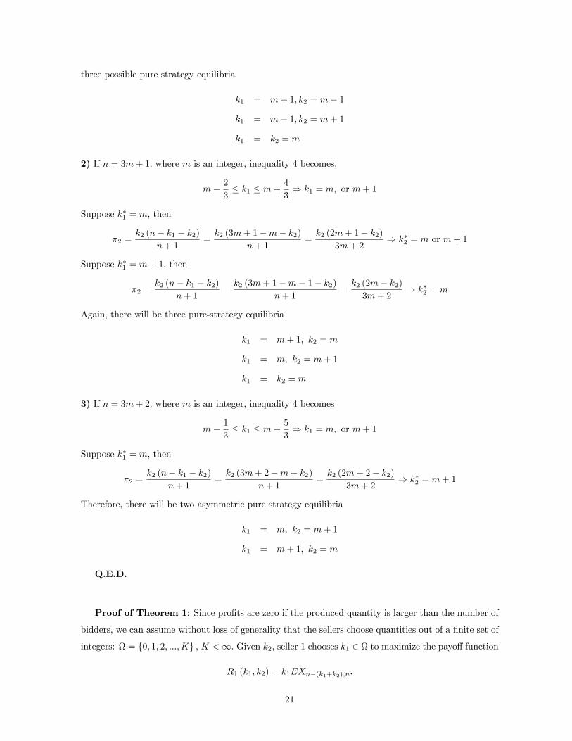
three possible pure strategy equilibria
k1 = m+ 1; k2 = m� 1
k1 = m� 1; k2 = m+ 1
k1 = k2 = m
2) If n = 3m+ 1; where m is an integer, inequality 4 becomes,
m� 23� k1 � m+
4
3) k1 = m; or m+ 1
Suppose k�1 = m; then
�2 =k2 (n� k1 � k2)
n+ 1=k2 (3m+ 1�m� k2)
n+ 1=k2 (2m+ 1� k2)
3m+ 2) k�2 = m or m+ 1
Suppose k�1 = m+ 1; then
�2 =k2 (n� k1 � k2)
n+ 1=k2 (3m+ 1�m� 1� k2)
n+ 1=k2 (2m� k2)3m+ 2
) k�2 = m
Again, there will be three pure-strategy equilibria
k1 = m+ 1; k2 = m
k1 = m; k2 = m+ 1
k1 = k2 = m
3) If n = 3m+ 2; where m is an integer, inequality 4 becomes
m� 13� k1 � m+
5
3) k1 = m; or m+ 1
Suppose k�1 = m; then
�2 =k2 (n� k1 � k2)
n+ 1=k2 (3m+ 2�m� k2)
n+ 1=k2 (2m+ 2� k2)
3m+ 2) k�2 = m+ 1
Therefore, there will be two asymmetric pure strategy equilibria
k1 = m; k2 = m+ 1
k1 = m+ 1; k2 = m
Q.E.D.
Proof of Theorem 1: Since pro�ts are zero if the produced quantity is larger than the number of
bidders, we can assume without loss of generality that the sellers choose quantities out of a �nite set of
integers: = f0; 1; 2; :::;Kg ; K <1: Given k2; seller 1 chooses k1 2 to maximize the payo¤ function
R1 (k1; k2) = k1EXn�(k1+k2);n:
21
and given k1; seller 2 chooses k2 2 to maximize the payo¤ function
R2 (k1; k2) = k2EXn�(k1+k2);n
Let � denote the above described two-person game, and de�ne
P (k1; k2) = k1k2EXn�(k1+k2);n
We now verify that P is an ordinal potential of �:17 We need to check that:
8k2 > 0; R1 (k1; k2)�R1 (k01; k2) > 0, P (k1; k2)� P (k01; k2) > 0
8k1 > 0; R2 (k1; k2)�R2 (k1; k02) > 0, P (k1; k2)� P (k1; k02) > 0
The above conditions become
k1EXn�(k1+k2);n � k01EXn�(k01+k2);n > 0, k1k2EXn�(k1+k2);n � k01k2EXn�(k01+k2);n > 0
k2EXn�(k1+k2);n � k02EXn�(k01+k2);n > 0, k1k2EXn�(k1+k2);n � k1k02EXn�(k01+k2);n > 0
which trivially hold.
Since both k1 and k2 are chosen from a �nite set ; it is obvious that the potential P has a maximum
on �: (Note that the maximum need not be unique). The existence result follows now directly from
the following result:
Lemma 8 (Lemma 2.1, Monderer and Shapley, 1996) Let P be an ordinal potential function for
�: Then the equilibrium set of � (R1; R2) coincides with the equilibrium set of � (P; P ) : That is,
(k1; k2) 2 � is an equilibrium point for � if and only if for every i 2 f1; 2g ;
P (ki; k�i) � P (k0i; k�i) for every k0i 2 :
Consequently, if P admits a maximal value in �; then � (R1; R2) possesses a pure strategy equilib-
rium.
Q.E.D.
Proof of Theorem 2: By the above proof, the potential P has a maximum. Suppose that this
maximum is achieved at (k�1 ; k�2) : We need to show that jk�1 � k�2 j � 1: Assume, by contradiction, that
the opposite holds:
jk�1 � k�2 j > 1
, jk�1 � k�2 j � 217 If the �rms face a marginal cost c > 0; de�ne the potential P (k1; k2) = k1k2(EXn�(k1+k2);n� c): This and the next
proof proceed then in an analogous fashion yielding the respective results.
22
Without loss of generality assume that
k�1 � k�2 + 2: (11)
Consider now (k01; k02) in � de�ned by
k01 = k�1 � 1
k02 = k�2 + 1
and observe that k01 + k02 = k
�1 + k
�2 : We obtain then that
P (k01; k02)� P (k�1 ; k�2)
= (k�1 � 1) (k�2 + 1)EXn�(k�1+k�2);n � k�1k�2EXn�(k�1+k�2);n
= (k�1 � k�2 � 1)EXn�(k�1+k�2);n > 0
where the last inequality follows by (11). This yields a contradiction to the assumption that P achieves
a maximum at (k�1 ; k�2) : Thus, jk�1 � k�2 j � 1 as desired. Q.E.D.
Proof of Proposition 4:
1) Suppose F is convex. Given k2; seller 1 chooses k1 to maximize
R1 = k1EX(n�k2)�k1;n
By Corollary 2, if F is convex, k1 � 12 (n� k2) : Analogously, we have k2 �
12 (n� k1) : Combining the
two inequalities, it follows that
k1 + k2 �2
3n
The opposite inequality holds for concave F:
2) Now suppose F is IFR and n is large. Given k2; seller 1 chooses k1 to maximize
R1 = k1EX(n�k2)�k1;n
By Corollary 1, we have k1 � 1e (n� k2) : Similarly, we have k2 �
1e (n� k1) : Therefore,
k1 + k2 �2
1 + en
The proof for the DFR case is analogous. Q.E.D.
Proof of Proposition 5: Suppose that m = n1 = n2 is large enough. Total revenue before the
merger is
�1 + �2 = 2maxkkF�1
�m� km
�Let k� 2 argmax kF�1
�m�km
�:
23
In the post merger competition the revenues are given by:
�c1 = �c2 = max
kikiF
�1�2m� ki � k�i
2m
�We focus on the (quasi) symmetric equilibrium in the post merger games (which always exists by
Proposition 2). The potential function is
P (k1; k2) = k1k2F�1�2m� k1 � k2
2m
�Since jkc1 � kc2j � 1, the pro�le (kc1; kc2) that maximizes the potential must satisfy
kci 2 argmax (k)2F�1
�m� km
�; i = 1; 2
One implication is that
kc1 62 argmax kF�1�m� km
�The change in total revenue is:
�c1 + �c2 � (�1 + �2)
= 2kc1F�1�m� kc1m
�� 2k�F�1
�m� k�m
�< 0
because k� 2 argmax kF�1�m�km
�: Thus, a merger reduces total revenue. Q.E.D.
Proof of Lemma 1: Fix a strategy pro�le for all agents except buyer h; and assume that in this
pro�le the respective quantities and number of bidders at each site are k1; k2; n1; n2; where n1 + n2 =
n� 1: Denote by X the random variable representing bidder h�s valuation. If h joins site i; i = 1; 2; his
expected payo¤ is given by
PrfX � EXni+1�ki;ni+1gE[X � EXni+1�ki;ni+1 j X � EXni+1�ki;ni+1]; i = 1; 2
It is immediate that the above expression is higher for i = argmin fEXn1+1�k1;n1+1; EXn2+1�k2;n2+1g;
thus it is optimal for bidder h to join the site with the lower expected price. The second argument
follows then immediately by the de�nition of equilibrium. Q.E.D.
Proof of Lemma 2:
1) Suppose without loss of generality that EXn1�k1;n1 � EXn2�k2;n2 . Since
EXn1+1�(k1+1);n1+1 = EXn1�k1;n1+1 < EXn1�k1;n1
we obtain
EXn1+1�(k1+1);n1+1 < EXn2�k2;n2
24
The last inequality provides a su¢ cient condition for a buyer to move from auction 2 to auction 1 if
seller 1 increases the supplied quantity by one unit while all other agents stay put.
2) Let n1 = m: By Lemma 5 in Appendix A, if F is IFR thenPr
1(m� i+ 1)(EXi;m � EXi�1;m)
is stochastically increasing in m � r: Let r = 1; then
mEX1;m < (m+ 1)EX1;m+1
Since EX1;m+1 < EX1;m; we have
(m� 1)EX1;m < mEX1;m+1
Similarly, by Lemma 5
EX1;m + (m� 1)EX2;m < EX1;m+1 +mEX2;m+1
Since EX2;m+1 < EX2;m; we have
(m� 2)EX2;m < (m� 1)EX2;m+1
By induction, for all 1 � i < m;
(m� i)EXi;m < (m� i+ 1)EXi;m+1
Letting i = m� k; we get
kEXm�k;m < (k + 1)EXm�k;m+1
The last inequality implies that a seller increases his revenue by attracting one more buyer from the
other site.
3) Suppose that the number of buyers in the auction is m: By Lemma 6, if F is IFR(DFR) then
(m� i+ 1)(EXi;m � EXi�1;m) is stochastically increasing (decreasing) in m � i for �xed i: Thus,
(m� i+ 2)(EXi;m+1 � EXi�1;m+1) > (m� i+ 1)(EXi;m � EXi�1;m)
This implies that
(m� i+ 2)EXi;m+1 � (m� i+ 1)EXi;m > (m� i+ 2)EXi�1;m+1 � (m� i+ 1)EXi�1;m
Since EXi;m+1 < EXi;m we obtain
(m� i+ 1)EXi;m+1 � (m� i)EXi;m > (m� i+ 2)EXi�1;m+1 � (m� i+ 1)EXi�1;m
Letting i = m� k; we get
(k + 1)EXm�k;m+1 � kEXm�k;m > (k + 2)EXm�k�1;m+1 � (k + 1)EXm�k�1;m
25
The last inequality implies that the marginal revenue of a seller that attracts one more buyer by
supplying one more unit is decreasing in k. Q.E.D.
Proof of Theorem 3:
As mentioned in the text, if both sellers make a pro�t in equilibrium, we must have k�1 + k�2 < n:
Assume that
c � mins2[1;n�1]; k2[0;s�1]
f(k + 1)EXs�k;s+1 � kEXs�k;sg
Then, no matter how many units are supplied, and how many bidders attend, it is always pro�table
for a seller to increase supply by one unit if he attracts one more buyer. By Lemma 2-3, we know that
marginal revenue is decreasing if F is IFR: Then, for each s; the minimum in the above condition is
achieved for k = s� 1 , and it is su¢ cient to assume that
c � mins2[1;n�1];
fsEX1;s+1 � (s� 1)EX1;sg
Suppose now, by contradiction, that (n�1; k�1 ;n
�2; k
�2) is an equilibrium, where n
�1; n
�2 > 0; n
�1+n
�2 = n;
k�1 ; k�2 > 0 and k
�1+k
�2 < n. Suppose also, without loss of generality, that seller 1 faces the lower expected
auction price. Then this seller can increase the number of supplied units to (k�1 + 1) : By Lemma 2, at
least one buyer will want to switch to his auction, and, by the assumption on the marginal cost c; this
constitutes a pro�table deviation. More buyers switching is even more pro�table since the price further
increases. Therefore, (n�1; k�1 ;n
�2; k
�2) cannot be an equilibrium.
Lemma 2 and condition (5) imply that a seller selling ki � n2 �1 objects to
n2 bidders has incentive to
increase his supply. But, if both sellers together sell n objects, they cannot both make positive pro�ts.
Q.E.D.
Proof of Proposition 6:
Under condition (7) both sellers have an incentive to increase supply from n2 � 2 to
n2 � 1; but no
seller has an incentive to increase supply from n2 � 1 to
n2 if by doing so only one more buyer will be
attracted. If a seller sells n2 � 1 units, at least
n2 � 1 buyers will attend his auction. Thus, no seller
can attract more than one buyer by increasing the number of supplied units beyond n2 � 1: Finally, no
seller has an incentive to decrease supply from k�i =n2 � 1 since a decrease by k units induces at least
k buyers to switch to the other auction. Q.E.D.
Proof of Proposition 7:
1) Assume that seller 1 sets k1 = n� 1: In that case, at least n1 = n� 1 will always attend auction
1, and the price in auction 1 is at most EX1;n . Seller 2 has no way of ensuring an equal or lower price.
Thus, no matter what seller 2 does, he cannot attract enough buyers, and entry is not pro�table.
26
Assume next that seller 1 sets k1 = n � 2: Given that at least n1 = n � 2 buyers always attend
auction 1, the only way in which seller 2 can make a pro�t is by auctioning one unit to 2 buyers. In
that case the price is EX1;2: By switching to auction 1, one of these two buyers will face a price of
EX1;n�1 < EX1;2: Thus, switching is pro�table, and seller 2 can never make a pro�t by entry.
Continuing in this way, let ek1 be the minimal k1 such that for all k2 < n� ek1, and for all n2; k2 <n2 < n� ek1; it holds that
EXn2�k2;n2 > EXn�n2+1�fk1;n�n2+1 > 0Assume then that k�1 � ek1; and assume that selling k�1 is pro�table for seller 1 (condition (8)) .Then,
the above inequality implies condition (9), and thus the existence of an equilibrium with a unique active
site.
The assumptions in the statement are satis�ed for su¢ ciently convex F and su¢ ciently small c by
Proposition 1.
2) Assume that k�1 <n2 : Setting k2 = k
�1 ; we obtain:
EXn2�k2;n2 � EXn�n2+1�k�1 ;n�n2+1 = EXn2�k�1 ;n2 � EXn�n2+1�k�1 ;n�n2+1
= EXn2�k�1 ;n2 � EXn2�k�1+(n�2n2+1);n2+(n�2n2+1) < 0
This follows because n� 2n2+1 > 0 (k2 = k�1 implies n1 = n2) and because EXi;j < EXi+a;j+a for all
i < j and a > 0: In particular, condition (9) cannot be satis�ed. Thus, by replicating seller 1�s strategy,
seller 2 can sustain a positive pro�t, and an asymmetric equilibrium with a unique active seller does
not exist.
The assumption k�1 <n2 is clearly satis�ed if F is su¢ ciently concave � see Proposition 1 and
Corollary 2. Q.E.D.
Proof of Proposition 8: Assume that total supply in monopoly is 2k units. Denote by g(x) =
(F�1)0(x): Then, the marginal revenue obtained by supplying an additional unit is given by:
MRM (k) = (2k + 1)EXn�(2k+1);n � 2kEXn�2k;n
= EXn�(2k+1);n � 2k�EXn�2k;n � EXn�(2k+1);n
�� F�1
�n� 2k � 1n+ 1
�� 2k
�F�1
�n� 2kn+ 1
�� F�1
�n� 2k � 1n+ 1
��
� F�1�n� 2k � 1n+ 1
��2kg
�n�2kn+1
�(n+ 1)
For the competition model with one auction site and total supply of 2k; the marginal revenue of a
27
seller is:
MRC1 (k) = (k + 1)EXn�(2k+1);n � kEXn�2k;n
= EXn�(2k+1);n � k�EXn�2k;n � EXn�(2k+1);n
�� F�1
�n� 2k � 1n+ 1
�� k
�F�1
�n� 2kn+ 1
�� F�1
�n� 2k � 1n+ 1
��
� F�1�n� 2k � 1n+ 1
��kg�n�2kn+1
�(n+ 1)
For the competition model with two sites and total supply 2k; assume that a seller attracts s
additional bidders by increasing supply by one unit. Then his marginal revenue is:
MRC2 (k) = (k + 1)EX(n2+s)�(k+1);n2+s
� kEXn2�k;
n2
By the assumption that equilibrium supply is at least n3 +2 units, and by Lemma 9 below, we get that
s = 1: This yields:
MRC2 (k) = (k + 1)EXn2�k;
n2+1
� kEXn2�k;
n2
= EXn2�k;
n2+1
� k�EXn
2�k;n2� EXn
2�k;n2+1
�� F�1
� n2 � kn2 + 2
�� k
�F�1
� n2 � kn2 + 1
�� F�1
� n2 � kn2 + 2
��� F�1
�n� 2kn+ 4
�� kg
� n2 � kn2 + 1
�� n2 � kn2 + 1
�n2 � kn2 + 2
�
= F�1�n� 2kn+ 4
��kg�n�2kn+2
�(n+ 2)
(n� 2k)�n2 + 2
�For large n we have
F�1�n� 2k � 1n+ 1
�� F�1
�n� 2kn+ 4
�kg�n�2kn+2
�(n+ 2)
�kg�n�2kn+1
�(n+ 1)
Therefore, we obtain
MRM (k) < MRC1 (k) and MRM (k) < MRC2 (k) for all k:18
On the other hand, note that(n� 2k)�n2 + 2
� > 1, k <n
4+ 1:
Thus, we have: 8<: MRC2 (k) < MRC1 (k) if k < n4 + 1
MRC2 (k) > MRC1 (k) if k > n4 + 1
:
18Note that the comparison among MRM (k) and MRC1(k) hold always, i.e., without any additional assumptions about
the number of bidders, supply, etc..
28
If the distribution F has an increasing hazard rate, then by Lemma 2, the marginal revenueMRC2(k)
is decreasing in k. Note also that
MRM (k) = EXi;n � (n� i+ 1) (EXi;n � EXi�1;n) where i = n� 2k
MRC1 (k) =1
2EXi;n +
1
2EXi�1;n �
1
2(n� i+ 1) (EXi;n � EXi�1;n) where i = n� 2k
By Lemma 7, both MRM (k) and MRC1 (k) are decreasing in k if F is IFR.
Since the marginal cost is assumed to be the same across models, the equilibrium quantity is lowest
and the price is the highest under monopoly. If marginal cost is relatively low, and assuming that an
equilibrium exists in the competition model with two sites, this situation is more competitive than the
one with one site. The opposite occurs for high marginal cost. Q.E.D.
When deriving the marginal revenue in the competition model with two auction sites, we assumed
that the additional number of bidders that a seller can attract by increasing supply by one unit is one.
The following lemma gives a mild condition under which this is indeed the case: It will be satis�ed as
long as c is not too large, such that the equilibrium supply of each seller satis�es k > n6 +1: Analogous,
weaker conditions can be derived whenever the number of attracted bidders is �nite and small relative
to the equilibrium quantity k:
Lemma 9 Consider the competition model with two auction sites (C2) for a large number of buyers n.
Suppose that the marginal cost c satis�es
c < (n
6+ 2)EX(n3�1;
n2+1)
��n6+ 1�EX(n3�1;
n2 )
(12)
Then, if a seller increases (decrease) supply by one unit, he attracts (looses) exactly one buyer;
Proof of Lemma 9: By the necessary condition for a symmetric equilibrium (6), and condition
(12), we obtain that k� > n6 + 1 where k
� denotes the equilibrium supply of each seller (otherwise, a
seller always has incentive to increase quantity by one).
1) Suppose �rst that seller 1 increases supply by one unit. Lemma 2 shows that he can attract at
least one more bidder. Therefore, we only need to show that he cannot attract two more bidders. That
is, we need to show that
EXn2+2�(k�+1);
n2+2
> EXn2�1�k�;
n2�1:
For large n; this is equivalent to showing
F�1� n2 + 1� k
�
n2 + 3
�> F�1
� n2 � 1� k
�
n2
�,
n2 + 1� k
�
n2 + 3
>n2 � 1� k
�
n2
,
k� >n
6+ 1:
29
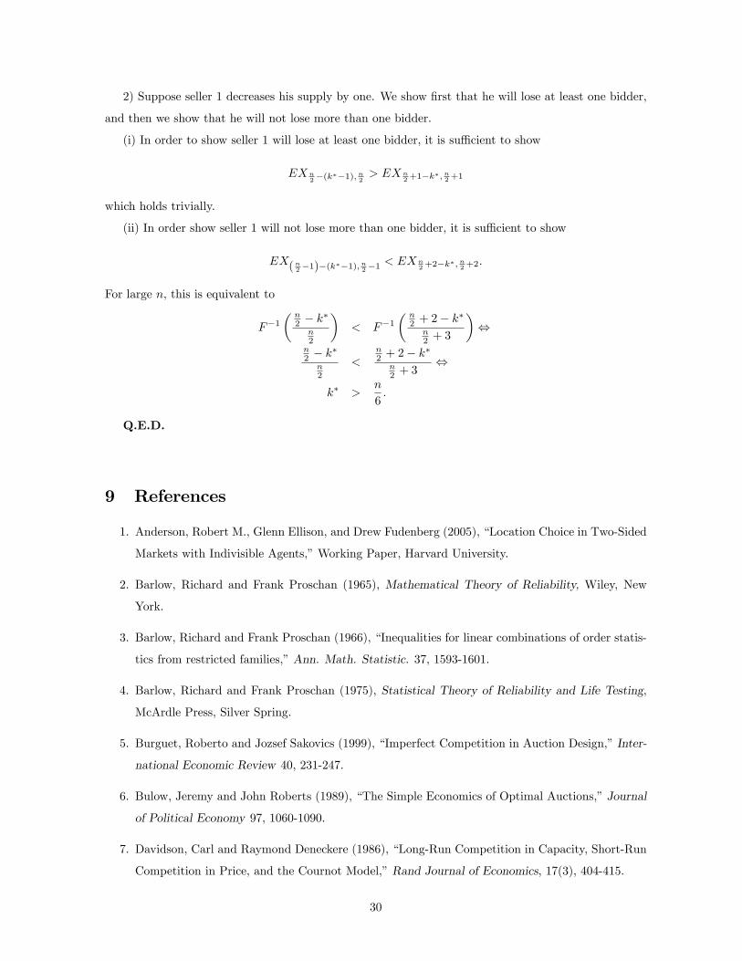
2) Suppose seller 1 decreases his supply by one. We show �rst that he will lose at least one bidder,
and then we show that he will not lose more than one bidder.
(i) In order to show seller 1 will lose at least one bidder, it is su¢ cient to show
EXn2�(k��1);
n2> EXn
2+1�k�;n2+1
which holds trivially.
(ii) In order show seller 1 will not lose more than one bidder, it is su¢ cient to show
EX(n2�1)�(k��1);n2�1
< EXn2+2�k�;
n2+2
:
For large n; this is equivalent to
F�1� n2 � k
�
n2
�< F�1
� n2 + 2� k
�
n2 + 3
�,
n2 � k
�
n2
<n2 + 2� k
�
n2 + 3
,
k� >n
6:
Q.E.D.
9 References
1. Anderson, Robert M., Glenn Ellison, and Drew Fudenberg (2005), �Location Choice in Two-Sided
Markets with Indivisible Agents,�Working Paper, Harvard University.
2. Barlow, Richard and Frank Proschan (1965), Mathematical Theory of Reliability, Wiley, New
York.
3. Barlow, Richard and Frank Proschan (1966), �Inequalities for linear combinations of order statis-
tics from restricted families,�Ann. Math. Statistic. 37, 1593-1601.
4. Barlow, Richard and Frank Proschan (1975), Statistical Theory of Reliability and Life Testing,
McArdle Press, Silver Spring.
5. Burguet, Roberto and Jozsef Sakovics (1999), �Imperfect Competition in Auction Design,�Inter-
national Economic Review 40, 231-247.
6. Bulow, Jeremy and John Roberts (1989), �The Simple Economics of Optimal Auctions,�Journal
of Political Economy 97, 1060-1090.
7. Davidson, Carl and Raymond Deneckere (1986), �Long-Run Competition in Capacity, Short-Run
Competition in Price, and the Cournot Model,�Rand Journal of Economics, 17(3), 404-415.
30
8. Demange, Gabrielle, David Gale and Marilda Sotomayor (1986), �Multi-Unit Auctions,�Journal
of Political Economy 94, 863-872
9. Dixit, Avinash (1980), �The role of investment in entry deterrence,�Economic Journal 90, 95�106.
10. Ellison, Glenn, Drew Fudenberg and Markus Mobius (2004), �Competing Auctions,�Journal of
the European Economic Association 2(1): 30-66.
11. Ellison, Glenn and Drew Fudenberg (2003), �Knife-Edge or Plateau: When Do Market Models
Tip?�Quarterly Journal of Economics, 118: 1249-1278.
12. Genesove, David (1995), �Price Sensitivity to Supply Traded under Alternative Mechanisms in
the New England Fish Industry,�mimeo, MIT.
13. Hansen, Robert (1988), �Auctions with Endogenous Quantity,�RAND Journal of Economics 19,
44-58
14. Hoppe, Heidrun, Benny Moldovanu and Aner Sela (2006), �Matching Contests for Uncertain
Partners,�working paper, Bonn University.
15. Klemperer, Paul (1987), �Markets with Consumers�Switching Costs,�Quarterly Journal of Eco-
nomics 102, 375-394
16. Klemperer, Paul and Meg Meyer (1989), �Supply Function Equilibria in Oligopoly with Demand
Uncertainty,�Econometrica 57, 1243-1277.
17. Koutsougeras, Leonidas (2003), �Non-Walrasian Equilibria and the Law of One Price,� Journal
of Economic Theory 108, 169-175.
18. Kreps, David, and Jose Scheinkman (1983), �Quantity Precommitment and Bertrand Competition
Yield Cournot Outcomes,�Bell Journal of Economics 14, 326�337.
19. Lengwiler, Yvan (1999), �The Multiple Unit Auction with Variable Supply,�Economic Theory
14, 373-392.
20. Maggi, Giovanni (1996), �Strategic Trade Policies with Endogenous Mode of Competition,�Amer-
ican Economic Review, 86(1), 237-258.
21. LiCalzi, Marco and Alessandro Pavan (2006), �Tilting the Supply Schedule to Enhance Compe-
tition in Uniform Price Auctions,�European Economic Review, forthcoming.
22. Mc Adams, David (2006),�Uniform Price Auctions with Adjustable Supply,� discussion paper,
MIT.
31
23. McAfee, R. Preston (1993), �Mechanism Design by Competing Sellers,�Econometrica, 61, 1281-
1312.
24. Moldovanu, Benny, Aner Sela and Xianwen Shi (2005), �Contests for Status,� working paper,
Bonn University.
25. Monderer, Dov and Lloyd S. Shapley(1996), �Potential Games,�Games and Economic Behavior
14, 124-143.
26. Moreno, Diego, and Luis Ubeda (2006), �Capacity Precommitment and Price Competition Yield
the Cournot outcome,�Games and Economic Behavior, forthcoming.
27. Neeman, Zvi and Nir Vulkan (2001), �Markets versus Negotiations: the Predominance of Cen-
tralized Markets,�mimeo
28. Peters, Michael and Sergei Severinov (1997), �Competition Among Sellers Who O¤er Auctions
Instead of Prices,�Journal of Economic Theory, 75, 141-179.
29. � and � (2006), �Internet Auctions with Many Traders.� Journal of Economic Theory, forth-
coming.
30. Schwartz, Jesse, and Richardo Ungo (2002), �Merging Auction Houses,�mimeo, Vanderbilt Uni-
versity.
31. Shapley, Lloyd and Martin Shubik (1975), �Trade Using One Commodity as a Means of Payment,�
Journal of Political Economy 85, 937-968.
32