1

Comparison of Welfare Results from Trade Liberalization in the

Armington, Krugman and Melitz Models: Impacts with features of real economies*

Edward J. Balistreri, Iowa State University

and

David G. Tarr, Former Lead Economist, The World Bank

June 26, 2017

Abstract: In this paper, we contribute to the literature about how the welfare effects of a reduction in

trade costs are impacted by market structure assumptions. We compare the Armington structure of trade

under perfect competition with the Krugman structure of trade under monopolistic competition and the

Melitz structure of trade under monopolistic competition with heterogeneous firms. Given its proven

importance to the welfare results, we hold the local trade response (as measured in gravity regressions)

constant across the model comparison exercise. We start with highly simplified versions of these models

where we reproduce the result of Arkolakis et al. (2012) that the welfare impacts are identical. We then

show that the welfare results of these models differ when we introduce several features that are important

to real economies, several of which have not yet been examined in the literature.

Keywords: heterogeneous firms, gains from trade, theory with numbers, exact hat algebra

JEL classification: F12, F18

*The authors gratefully acknowledge support from the World Bank Research Committee under grant RF-P159745-

RESE-BBRSB for the project entitled "How Large are the Welfare Impacts of the Heterogeneous Firms Model:

Results from an assessment of the Trans-Pacific Partnership and from a Stylized Model." We thank Maryla

Maliszewska, Russell Hillberry and Aaditya Mattoo for comments. The views expressed are those of the authors and

do not necessarily reflect those of the World Bank, its Executive Directors or those acknowledged.

2

Contents 1. Introduction ........................................................................................................................................... 3 2. Literature Review .................................................................................................................................. 5

2.1 Rationales for the Gains from Trade ................................................................................................... 5 2.2 Exact Hat Literature for Welfare Calculations .................................................................................... 6

2.2.1 Summary of Established Results. ................................................................................................. 6 2.2.2 Does the Exact Hat Methodology Offer a Highly Parsimonious Approach for Calculating the

General Equilibrium Welfare Gains from a Reduction in Trade Costs. ............................................... 7 2.3 CGE literature on the welfare gains from trade liberalization (a brief overview)............................... 9

3. Armington, Krugman and Melitz Model Structures ........................................................................... 10 3.1Armington Structure .......................................................................................................................... 10 3.2 Krugman Structure ............................................................................................................................ 11 3.3 Melitz Structure................................................................................................................................. 12

4. Gravity, Trade and FDI Responses and Calibration Strategy ................................................................. 13 4.1 Gravity-equation Estimation and Trade Responses .......................................................................... 13 4.2 Gravity Equation Estimation of the FDI Response .......................................................................... 16 4.3 Intermediate Demand Structures ....................................................................................................... 17

4.3.1 Cobb-Douglas Demand with data on intermediate use. ............................................................. 17 4.3.2 Cobb-Douglas Demand with an aggregate intermediate good. .................................................. 18 4.3.3 Leontief Demand for Intermediates with actual data on intermediate use. ............................... 19 When we have Leontief demand for intermediates, we have that output is: ...................................... 19

5. Computational Simulations ..................................................................................................................... 19 5.1 Model with One Sector, One Factor, No Intermediates and Balanced Trade ................................... 19 5.2 Trade Imbalances, Intermediate Goods and Multiple Sectors .......................................................... 19

5.2.1 Trade Imbalances. ...................................................................................................................... 20 5.2.2 Intermediates. ............................................................................................................................. 20 5.2.3. Multiple Sectors with Intermediates. ........................................................................................ 20

5.3 Impact of Alternate Structures for Intermediate Demand ................................................................. 21 6. Conclusion .............................................................................................................................................. 23 References ................................................................................................................................................... 24

Table 1: Literature Results on the Ranking of Welfare Gains in the Armington, Krugman and Melitz

Models ..................................................................................................................................................... 28 Table 2: Basic Model Equivalence of Welfare Results Across Market Structures and Replication of

Exact Hat Calculations--Model with One Sector, One Factor, No Intermediates and Zero Trade

Balance. ................................................................................................................................................... 29 Table 3: Impact of Incorporating Trade Imbalances, Intermediates and Multiple Sectors ..................... 30 Table 4: Impact of Intermediate Modeling Structure: (1) Single Composite Intermediate; (2) Cobb-

Douglas Demand; or (3) Leontief Demand ............................................................................................. 30

3

1. Introduction

In this paper, we contribute to the literature on how the welfare effects of a reduction in trade

costs are impacted by market structure assumptions. We compare the Armington (1969) model of trade

under perfect competition with the Krugman (1980) model of trade under monopolistic competition and

the Melitz (2003) model of trade under monopolistic competition with heterogeneous firms. We

contribute to the literature on how the welfare results depend on market structure when we introduce

several model features that are important in applications to real economies, but which have not yet been

investigated.

We start with highly stylized versions of these models where we reproduce the result of Arkolakis

et al. (2012) that the welfare impacts are identical. In that stylized model Arkolakis et al. (2012) assume:

the model contains one sector per country; has one factor of production; does not contain intermediates;

there is no labor-leisure choice; trade of each country is balanced; there is no foreign direct investment;

trade costs are iceberg and the trade shock moves the economy to autarky.1 In an excellent follow-up

paper, Costinot and Rodriguez-Clare (2014) highlight and clarify the impact of relaxing several of the

rather restrictive assumptions of the simple model of Arkolakis et al. (2012). Regarding their more

realistic non-autarky comparative static exercises, they provide comparisons across market structures in

models that include multiple sectors, a single aggregate tradeable intermediate good (where all sectors use

intermediates in the same proportion) and changes in uniform tariffs; these models start from zero tariffs

and zero trade balances. Our paper provides new results for the impact of the Armington, Krugman and

Melitz market structures in multi-sector models that include: (i) intermediates with demand structures that

reflect actual data on intermediate use; (ii) the impact of alternate model structures for intermediates; (iii)

heterogeneous tariffs across sectors; (iv) examination of tariff changes without assuming a movement

either from free trade or to autarky; (v) foreign direct investment (FDI); (vi) specific factors of

production; (vii) trade imbalances; and (viii) import of primary factors such as specialized intermediate

inputs.2

The work of Arkolakis, Costinot and Rodriguez-Clare provides significant guidance for future

numerical evaluation of welfare impacts of trade costs. Beyond the fact that it enhances our understanding

of the sources of welfare impacts across the different structures, it provides a concrete link between

econometric and computational models. They show the importance of grounding numerical model

1 If fixed exporting costs are paid in the destination country, it is not necessary to assume a movement to autarky. 2 Costinot and Rodriguez-Clare (2014) address some of these issues under perfect competition. In particular, using

the Armington model, they assess the impact of trade imbalances, heterogeneous tariffs across sectors, and

intermediates with demand structures that reflect actual data. However, the relative impact of the Krugman or Melitz

structures with these extensions that are an open question.

4

responses in the extensive literature on trade responses as measured using gravity models. In this paper,

we parameterize each of our models in a way that is consistent, to the extent possible, with the estimated

trade response from the gravity equations. Consequently, our comparisons of the Armington, Krugman,

and Melitz models maintain consistent trade responses. Further, when we introduce FDI into the model,

our models are the first to also hold the FDI response constant across the models to be consistent with

econometric estimates of the responsiveness of investment to a reduction in barriers. The FDI response is

a second constraint on the calibration of the elasticities of the model in addition to the trade response.

We begin our analysis by eliminating most of the details of the GTAP data to produce a model

consistent with the simplest model of Arkolakis et al. (2012) (including untruncated Pareto productivity

distributions). We first replicate the Arkolakis et al. (2012) equivalence result, then progressively

introduce real features of the data. We find that trade imbalances alone are insufficient to break the

equivalence result of Arkolakis et al. (2012). The introduction of intermediates in a single sector, one

factor model with trade imbalances results, in all our simulations, in larger gains in the Melitz model than

in the Krugman model and larger gains in the Krugman model than in the Armington model. If we add

multiple sectors to the model with intermediates and trade imbalances, the ranking of Melitz greater than

Krugman greater than Armington tends to hold. But there are terms of trade effects in the monopolistic

competition models that significantly reverse that ranking for at least one of our ten regions. We show

that the structure of intermediate demand and the use of real data on intermediate factor shares by sector

make a significant difference in the comparative results across the models. With Cobb-Douglas

intermediate demand and real data, we find that, for the average for the world, the ranking of the welfare

gains is: Melitz larger than Krugman and Krugman larger than Armington. Leontief intermediate demand

diminishes the impact of market structure so that, regarding the average for the world, there is no

difference in the estimated welfare gains across market structures. However, the comparative ranking

among the three models is not fully consistent across the ten regions, indicating that the ranking of the

welfare results between Melitz, Krugman and Armington is parameter dependent.

The exact hat methodology for welfare calculations elaborated by Arkolakis et al. (2012) yields

the parsimonious two parameter welfare calculation in their simple model. Costinot and Rodriguez-Clare

have shown, however, that their exact hat calculation expands to a system of several thousand non-linear

independent equations when a modest number of realistic features are introduced into their multi-region

model. To date, the exact hat literature has not provided solutions for either of the monopolistic

competition general equilibrium models with the more realistic features of the data are real economies,

such as data on intermediate factor shares by sector with multiple sectors, trade imbalances, or non-zero

initial tariffs. Most of these real economy features have been solved by the exact hat literature only in

5

perfect competition models. Therefore, there are many unanswered questions on the relative welfare

impact of the Armington, Krugman and Melitz to which this paper contributes.

In section 2, we summarize the literature, with a focus in section 2.2 on what we know about the

comparative welfare gains of the Armington, Krugman and Melitz models. This includes a discussion of

how parsimonious is the exact hat calculus when realistic features of an economy are introduced. We

present the equations of the model is section 3. In section 4, we discuss how we calibrate the trade

response and the FDI response based on gravity models. We also describe the intermediate demand

structure of Costinot and Rodriguez-Clare (2014) and two alternate measures that use real data on

intermediates. We present the results of the simulations in section 5 and conclude in section 6.

2. Literature Review

2.1 Rationales for the Gains from Trade

One of the oldest propositions in economics is that there are gains from international trade. Ricardo

(1817) elucidated the principle of comparative advantage as the source of gains from international trade

and Samuelson (1939) established it rigorously. Krueger (1974) and Bhagwati (1982) showed that in the

presence of "rent-seeking" the gains from trade liberalization would be significantly larger than from

specialization gains from comparative advantage.3 Since 1979, numerous authors showed that under

conditions of increasing returns to scale and imperfect competition, the gains from trade liberalization

could be larger than under perfect competition for multiple reasons. The reasons included: (i) increased

competition from international trade could lower markups, which would lead to rationalization gains as

firms slide down their average cost curves, Krugman (1979); (ii) additional varieties in monopolistically

competitive markets are a source of gains from trade, Krugman (1980); (iii) international trade could add

additional varieties of intermediate inputs, Ethier (1982); (iv) foreign direct investment of multinationals

could be a source of significant gains from trade in imperfectly competitive markets, especially in

producer services markets, Markusen(1989; 2002), Markusen and Venables (1998); and Ethier and

Markusen (1996). Beginning with Melitz (2003), many theoretical papers have emphasized the

heterogeneous nature of firms in a monopolistic competition framework.4 These models of heterogeneous

firms provide a further rationale for the gains from international trade, as the endogenous decisions of

firms to enter or exit could lead to an increase in output by the more efficient firms and an increase in the

gains from trade. Following the Melitz (2003) paper, there has been a substantial increase in research in

international economics based on firm level data sets. Several new stylized facts about international trade

3 Bhagwati used the term "directly unproductive profit-seeking" activities.

4 See, for example, Arkolakis et al. (2008) and Bernard, Redding and Schott (2007).

6

have been identified, including that only the most productive firms export and trade liberalization induces

an intra-industry reallocation of resources.

2.2 Exact Hat Literature for Welfare Calculations

2.2.1 Summary of Established Results. In their influential paper Arkolakis et al. (2012)

construct stylized versions of the Armington, Krugman, and Melitz models. The surprising result they

found in their simplest model was that the welfare impacts of reducing trade costs were equivalent across

the three models. The simplifying assumptions of their simplest model include: it contains one sector per

country; has one factor of production; does not contain intermediates; there is no labor-leisure choice;

trade of each country is balanced; and there is no foreign direct investment. They show, under the

restrictions of their simplest model, that the welfare gains from trade depend on only two statistics:

changes in the domestic trade share (the “trade response”) and the elasticity of trade with respect to

variable trade costs. Their analysis is based on the "exact hat" methodology.5 Crucial to their result is the

argument that given the wide acceptance of gravity models in international trade and importance of the

trade response to the welfare results, the structural parameters of the three models must be adjusted to

yield trade responses consistent with gravity models. Estimation of the gravity model yields an estimate

of the trade elasticity, which determines the trade response and is important for the welfare calculation.

Balistreri, Hillberry and Rutherford (2010) were the first to point out that the Arkolakis et al.

(2010; 2012) result in their highly stylized model was very fragile. They showed that the introduction of a

labor-leisure choice (which in their model is equivalent to a second sector) would break the equivalence.

They noted that, in addition to multiple sectors, intermediates would break the equivalence in the welfare

results. This was also shown by Arkolakis, Costinot and Rodriguez-Clare (2012), who showed that with

intermediates, the monopolistic competition models produce larger gains from trade liberalization than

the perfect competition model. Melitz and Redding (2015) show that the Arkolakis et al. (2012)

equivalence result in the highly stylized one sector model fails to hold if the Pareto distribution of

productivity has a finite upper bound. Melitz and Redding find in that model that the endogenous

decisions of heterogeneous firms to enter and exit the market provide "an extra adjustment margin" that

augments the gains from international trade compared to a Krugman style homogeneous firms model. In

their model, there are larger welfare gains from reductions in trade costs and smaller welfare losses from

increases in trade costs. The generality of the Melitz and Redding result, regarding the welfare dominance

5 The term "exact-hat" refers to the characterization of equilibrium impacts in proportional changes. That is, if v̂ is

the change in a variable denoted in the benchmark and counterfactual as v and v′, respectively, then v̂ can be

summarized as ˆ '/v v v . See Dekle, Eaton and Kortum (2008) for an earlier application of the exact hat

methodology.

7

of the model with heterogeneous firms and a truncated Pareto distribution, has not yet been examined in

models with more general and realistic features.

Costinot and Rodriguez-Clare (2014) provide the most comprehensive investigation of the

relative welfare impacts of Armington, Krugman and Melitz models. They begin in their section 3 with

autarky exercises, where they examine the impact of relaxing some of the simplifying assumptions of the

one sector model of Arkolakis et al. (2012). With multiple sectors, but no intermediates and zero trade

imbalances, they show that there are no selection effects in these autarky exercises, so the Melitz and

Krugman model results are identical. In their 34 regions and 31 sectors numerical model, they find that

the relationship between the monopolistic competition models and the Armington model is ambiguous

(Costinot and Rodriguez-Clare, 2014, 214-215). Using their 34 regions, 31 sectors model, Costinot and

Rodriguez-Clare (2014, 219-220) consider a single aggregate intermediate good without real data (where

all sectors use intermediates in the same proportions) and find that the Melitz model produces larger

welfare gains than the Krugman model which, in turn, produces larger gains than the Armington model.

Costinot and Rodriguez-Clare (2014, section 4) assess tariff changes, rather than movements to

autarky, what they refer to as their richer comparative static exercises. They compare the welfare effects

of imposition of a uniform tariff in a model with ten regions, sixteen sectors, a single aggregate

intermediate good without real data (where all sectors use intermediates in the same proportions), a single

primary factor of production, zero trade balances and zero initial tariffs. In this model, Costinot and

Rodriguez-Clare find that with multiple sectors, losses of the uniform tariff tend to be larger in the

Krugman model compared with Armington (with exceptions), but are slightly lower in the Melitz model

compared with Krugman. With a single aggregate intermediate, the losses are greatest in the Melitz

model, next highest with Krugman and lowest with Armington (with some exceptions).

In summary, the literature to date indicates that the welfare ranking of Melitz to Krugman varies

with the model, the region and the nature of the counterfactual experiment. As we elaborate in section

2.2.2 below, the literature to date has not shown the impact of the Armington, Krugman or Melitz models

with heterogeneous tariffs, intermediates with real data on intermediate factor proportions, the impact of

either Cobb-Douglas or Leontief demand for intermediates, trade imbalances, specific factors, multiple

factors of production or foreign direct investment. In table 1, we summarize the literature results on

comparing the three market structures, prior to this paper.

2.2.2 Does the Exact Hat Methodology Offer a Highly Parsimonious Approach for

Calculating the General Equilibrium Welfare Gains from a Reduction in Trade Costs. Part of the appeal of the exact hat calculus in Arkolakis et al. (2012) was that the general

equilibrium welfare calculation could be calculated from two statistics: changes in the domestic trade

share (the “trade response”) and the elasticity of trade with respect to variable trade costs. In the case of

an autarky exercise, the trade response is dependent only on initial data, so there is no need for a model to

8

make the calculation. However, just as the equivalence of the welfare impacts across the three market

structures in the highly stylized model of Arkolakis et al. (2012) is very fragile, the sufficiency of the two

statistics for the welfare calculation is also very fragile. In fact, although Costinot and Rodriguez-Clare

succeed in defining equilibrium conditions for a general equilibrium trade model with realistic features,

they have numerically solved their general model only for a special case.

To be more specific, in their online appendix, Costinot and Rodriguez-Clare (2013, pp.9-10)

develop equilibrium conditions for a model with ten regions and sixteen sectors with realistic economy

features. Their multi-sector theoretical model (of their section 4) allows tariff changes that potentially

vary by sector and region, includes intermediates with intermediate factor proportions varying by sector

and includes unbalanced trade. Importantly, the exercises are comparative static, rather than movements

to autarky. They show that they this model is a system of 23 2nS n S simultaneous independent non-

linear equations, where S is the number of sectors and n is the number of regions. For the model with 10

regions and 16 sectors they employ, this is 3680 independent non-linear equations. If the number of

regions is 15, this is 7920 independent nonlinear equations. Although with their autarky exercises,

Costinot and Rodriguez-Clare consider 34 regions and 31 sectors, they reduce the model to 10 regions

and 16 sectors “to ease the computational burden.” When they solve a version of this model for the

Melitz, Krugman and Armington cases, they make the following simplifying assumptions: (i) there is an

aggregate intermediate good where all sectors consume intermediate factors in the same proportion (see

section 4.2.2 below for details); (ii) all tariffs are zero in the initial equilibrium; (iii) only a change in

uniform tariffs is considered; (iv) all trade balances are zero.

Costinot and Rodriguez-Clare subsequently assess the impact of relaxing assumptions by

assessing in their Armington model only: trade balances different from zero initially; heterogeneous tariff

changes; and multiple factors of production. The subsequent evaluations of Costinot and Rodriguez-Clare

are useful for understanding impacts in the Armington model. Crucially, however, despite showing the

results for the ranking of the welfare results across the three market structures in a model with several

simplifying assumptions, and then assessing the impact of simplifying assumptions in a perfect

competition model, to date the impacts of these simplifying assumptions have not been evaluated in the

Krugman or Melitz models and not been compared to Armington. The results in table 4 below for China

and the United States, provide examples that the impact of the simplifying assumptions in the Armington

model could have an opposite impact in the Krugman or Melitz model. Knowledge of the impact of a

modeling assumption in the Armington model is insufficient to infer the impact of the same modeling

assumption in the Krugman or Melitz models. Consequently, in our summary table of known results from

the literature, we do not report comparative results across these three market structures for the more

complicated model features.

9

To date, without assuming movements to autarky, the exact hat methodology has not yet

produced solutions to the Melitz or Krugman models with realistic features of economies, including

actual initial data on tariffs, real data on intermediates in multi-sector models and trade imbalances. Thus,

it remains to be shown that the exact hat approach offers a significantly simpler method for calculating

the welfare impacts of trade cost changes in realistic monopolistic competition models compared with

models defined in levels. Further, the exact hat methodology of Costinot and Rodriguez-Clare (2014)

comes at the cost of losing much sector and factor detail.

2.3 CGE literature on the welfare gains from trade liberalization (a brief overview)

The early CGE literature was based on constant returns to scale models, where the gains were

based on comparative advantage and calculated from "Harberger triangles." The estimated gains from

trade liberalization were sometimes characterized by the "Harberger constant," i.e., the gains were

generally less than one percent of GDP from trade liberalization. Among others, de Melo and Tarr (1990)

and Jensen and Tarr (2003) showed that, even in a perfect competition constant returns to scale model, if

there were rents involved, the gains could be many multiples of the gains from the "Harberger triangles."

Regarding imperfect competition models with homogeneous firms, the path breaking article was by

Harris (1984), who showed that the gains might be much larger if the behavioral interaction of

oligopolists is altered by the trade policy. Harrison, Rutherford and Tarr (1997) estimated that the impact

of rationalization gains (sliding down the average cost curve) were small in a quantity adjusting model of

oligopoly. Rutherford and Tarr (2002) showed that in a fully dynamic model based on Paul Romer style

endogenous growth with gains from variety, the gains from trade liberalization would be many multiples

of the gains in a model with constant returns to scale. Markusen, Rutherford and Tarr (2005) and

Rutherford and Tarr (2008) showed that introducing foreign direct investment in services with Dixit-

Stiglitz endogenous productivity effects would substantially increase the welfare gains. Francois,

Manchin and Martin (2013) have summarized many approaches to modeling market structure in CGE

models and suggested ways that the alternate model structures could be tested.

Regarding heterogeneous firms, the first effort at a CGE model was by Zhai (2008). His model was

developed into an application to the Trans Pacific Partnership in Petri, Plummer and Zhai (2012) and

employed in the Global Economic Prospects of the World Bank (2016). Unlike the Melitz model,

however, neither Zhai’s model, nor the model of Petri, Plummer and Zhai, allow entry or exit of firms,

nor does it allow uncertainly about the productivity (Zhai, 2008, pp. 7, 8). But their models do allow

existing firms to enter new markets and that type of entry creates a new variety and a welfare gain. Since

domestic firms face increased competition from foreign entry, some would be expected to exit. The model

of Zhai, however, does not allow firm exit; consequently, the model exaggerates the variety externality.

This explains why Petri, Plummer and Zhai obtain such large increases in the variety externality in their

10

model. Dixon, Jerie and Rimmer (2015) developed a stylized CGE model in which the Armington,

Krugman and Melitz models are special cases. As in the simplest Arkolakis, Costinot and Rodriguez-

Clare model, they find equivalent welfare results across market structure assumptions when the trade

response is held constant across the models. Their model, however, is not applied to data from an actual

economy or economies; in particular, all sectors in their model have identical factor shares, both within

and across countries. As discussed above, several papers have shown that the equivalence results found

by Dixon, Jerie and Rimmer (2015) fail to generalize when more complex features of actual economies

are brought into the model. The first CGE model of real economies consistent with the full Melitz

structure is Balistreri, Hillberry and Rutherford (2011). In their multi-region model they find that the

welfare gains from tariff reductions are several times larger than with an Armington trade model.

Balistreri, Hillberry and Rutherford (2011), however, did not hold the trade response constant across the

market structures. Recently other authors have adopted a computational setting for welfare analysis in

advanced frameworks with heterogeneous firms. The paper by Caliendo, Feenstra, Romalis and Taylor

(2015) is a good example. Their approach is in the tradition of solving models in percentage change

(exact-hat algebra); as we discussed above in reference to the approach of Arkolakis et al. (2012), it first

involves solving a system of independent, non-linear equations similar to modern CGE analysis.

3. Armington, Krugman and Melitz Model Structures

Consider a world economy with goods ,i I regions ,r R and factors .f F Now let us

indicate the trade structures applied to each good using subsets of I : Armington goods are indexed by ;

j J I ; Krugman goods are indexed by ;k K I and Melitz goods are indexed by .m M I

Abstracting from the broader general equilibrium, let ,i rQ be the total quantity demanded (absorption) of

the composite good i (made up of domestic and imported varieties) in region r , and let irY be the gross

output of good i in region r. In the context of the monopolistic competition structures, output, irY , is a

composite input commodity used by firms with a simple increasing-returns technology. With total

demand and supply of each good (or composite input) well specified we can focus on a description of the

trade equilibria across structures.

3.1Armington Structure

Consider that the composite good, satisfying demand ,i rQ is an optimal CES aggregate of

domestically supplied and imported goods. This is typically indicated as the Armington aggregation. It is

convenient to represent this aggregation using a dual unit cost function. The dual representation

11

simultaneously embeds the technology and optimization. Let jsP be the minimized unit cost (true price

index) of composite commodity j available in region s, and let jrc be the price of regionally differentiated

goods sourced from r. The CES unit cost function is given by:

1/(1 )

1( ) .

jj

js r jrs jrP c

,

where jrs is the iceberg trade-cost factor and j is the elasticity of substitution. Demand for the

domestic and each imported variety can be derived by applying Shephard’s lemma to the unit cost

function scaled up by the activity level given by jsQ . Summing across demand from all trade partners we

have the market clearance condition for output of good j from region r:

, .

j

js

jr s jrs j s

jrs jr

PY Q

c

This completes the Armington trade formulation. Gross output from region r is exhausted on demand

from each bilateral link, and it is assumed that the aggregation of imports and domestic goods occurs via a

CES activity.

3.2 Krugman Structure

Under the Krugman structure the aggregation is also CES, but it is assumed that the varieties are

distinguished at the firm level. Each region r has a number of firms measured by mass krN producing

commodity k. Let us denote krsp as the, gross of trade and transport-cost, price charged in market s by

each of the symmetric firms from region r. Firms are assumed to produce under an increasing returns

technology with a fixed cost and constant marginal cost.

Similar to the Armington aggregation the dual function that embeds the technology and optimization is

given by

1/(1 )

1,

kk

ks r kr krsP N p

.

In this case we use Shephard’s lemma to derive firm-level demand:

.

k

kskrs ks

krs

Pq Q

p

This demand function has a constant elasticity of k . We assume that each firm is small in that, from the

firm’s perspective, the price index ( ksP ) is not affected by the firm’s decision on its own price krsp .

12

Inclusive of iceberg transport costs the firm optimally prices in each market according to the standard

optimal markup:

.1 1/

krs krkrs

k

cp

Under an assumption of free entry firm profits from each market (s) will just cover the cost of entry:

.krs krskr k s

k

p qc f

The final equilibrium condition for the Krugman structure is market clearance for output of the

composite-input commodity k in region r. Output of composite-input commodity k is used by each firm

to cover fixed and variable cost (inclusive of iceberg trade costs). Considering the number of firms

operating the market clearance condition is given by

.kr kr k s krs krsY N f q

3.3 Melitz Structure

The Melitz structure follows closely the Krugman structure, but because firms face a set of, ex post,

different technologies (marginal costs) the equilibrium includes a number of extensions. These

extensions are simplified by defining the equilibrium in terms of a representative firm (following Melitz,

2003). Consider the price index defined on the price of the representative firm:

1/(1 )

1.

hh

hs r hrs hrsP N p

,

where the measure of the number of firms now tracks the number of firms operating on a given bilateral

link. Just as in the Krugman model firm level demand is given by

h

shrs hs

rs

Pq Q

p

. Optimal pricing follows with the inclusion of hrs as the measure of the

representative firm’s productivity.

.(1 1/ )

hr hrshrs

hrs h

cp

Under a Pareto distribution of productivity draws (with shape parameter a) we can represent the zero-

cutoff-profits condition in terms of the representative firm:

( 1 )

.hhr hrs hrs hrs

h

ac f p q

a

This condition indicates that out of the mass of available firms ( hrM ), those selecting into market s must

earn non-negative profits. The marginal firm earns zero profits and we relate the revenues of the marginal

13

to the representative firm through the Pareto distribution. While operating firms earn profits, in

expectation, free entry insures zero profits. A firm that enters can expect to earn the profits of the

representative firm weighted by the probability of operating in that market ( /hrs hrN M ). These expected

profits must cover the annualized sunk cost of entry. The free entry condition is thus given by

( 1)h hrs

hr hrs s hrs hrs

h hr

Nc f p q

a M

where is the probability that firm fails to survive into the next year. Next, we must determine the

productivity of the representative firm. Under the Pareto distribution (with support b) and operating firms

and entered firms determined by the zero-cutoff-profit and free-entry conditions the representative firm’s

productivity is given by

1/( 1) 1/

.1

h a

hrshrs

h hr

Nab

a M

Finally, we have the market clearance condition for output of composite-input commodity h in region r

.hrs hrshr hrs hr s hrs hrs

hrs

qY f M N f

Composite inputs are used to cover sunk, fixed-operating, and variable costs.

4. Gravity, Trade and FDI Responses and Calibration Strategy

4.1 Gravity-equation Estimation and Trade Responses

Our intent is to estimate trade responses directly from the GTAP 9 data using current structural-

gravity techniques. We take parameters based on econometric estimates for the Melitz model and adjust

elasticities in the Krugman and Armington model so that the trade response is the same.

To be precise, let W indicate the share of global expenditures that are spent on goods that are

produced in their respective home region:

,

,r rr

r s sr

W

X

X

where srX is the total value of country r's expenditures on goods from country s. If W is the domestic

trade share in the benchmark data and W is the domestic trade share in the in the counterfactual

equilibrium, then 1 W is the percentage change in the global trade share where ˆW is defined by:

14

ˆ .WW

W

Note that in the special case of a movement to autarky, in the counterfactual, ' 1W . Then ˆ 1W

W

and

the change in the trade response may be calculated from initial data and the trade elasticity without the

need of a model. We adjust the Armington and Krugman elasticities to match the observed percentage

increase in global trade intensity from the Melitz model. This gives us a fair comparison across structures

where they are parameterized to generate an equivalent aggregate trade response.

The calculation of the trade response is nontrivial in a multi-sector model. Although the trade

response is unique in a one sector model, and may be calibrated consistent with a unique trade elasticity

from a gravity model, in a multi-sector model, there are trade responses in each sector. Further, depending

on model assumptions, the trade elasticity may not be constant.6 In this paper, we hold the aggregate trade

response constant across the Armington, Krugman and Melitz models, which means that trade responses

at the sector level are not necessarily constant across the models.

For the Pareto distribution shape parameter in the Melitz model, we choose the value 4.58 from

the structural estimation of Balistreri, Hillberry and Rutherford (2011). Arkolakis et al. (2012) have

shown that in the one sector Melitz model, the Pareto shape parameter is equal to the trade elasticity; in

particular, the trade elasticity is independent of the Dixit-Stiglitz demand elasticity. The Dixit-Stiglitz

elasticity remains relevant, however, in models with realistic features as it affects the value to consumers

of additional varieties. For the value of the Dixit-Stiglitz trade elasticity in the Melitz model, we take the

value of 5.0 that Hillberry and Hummels (2014, p.1240) report as the median estimate from cross section

and panel estimates.

For the Krugman model, we adjust the Dixit-Stiglitz elasticities of substitution so that the trade

response is the same as in the Melitz model. The selection effect magnifies the trade response in the

Melitz model, but this effect is absent in the Krugman model. To obtain the same trade response in the

Krugman model as in the Melitz model, we must impose larger Dixit-Stiglitz elasticities. This means that

the value of an additional variety will be greater in the Melitz model compared to the Krugman model.

This will be important in interpreting our numerical results.

By similar reasoning, to hold the trade response constant, we find that we must choose the

Armington elasticities of substitution to be larger than the Dixit-Stiglitz elasticities of the Melitz model.

In the Melitz model, the value of 4.58 for the shape parameter and 5.0 for the Dixit-Stiglitz elasticities are

6 Melitz and Redding (2015) showed that the "existence of a single constant trade elasticity and its sufficiency

property for welfare are highly sensitive to small departures from those Arkolakis, Costinot and Rodriguez-Clare

parameter restrictions."

15

invariant across the scenarios. In the case of the Armington and Krugman models, the Armington and

Dixit-Stiglitz elasticities vary with the scenario, and those values are in the tables of results.

In an effort to keep the love of variety effect constant in the Krugman and Melitz models, one

might consider the following alternate calibration strategy. We would start with the Krugman model and

calibrate the Dixit-Stiglitz elasticities of substitution to be consistent with an estimate of the trade

elasticity from a gravity model. Then we would attempt to impose those same Dixit-Stiglitz elasticities of

substitution in the Melitz model so the love of variety effect is held constant. To hold the trade response

in the Melitz model consistent with the gravity estimate, we would then attempt to adjust the Pareto shape

parameter in the Melitz model to achieve a trade response in the Melitz model consistent with the trade

elasticity from gravity. The problem we encountered with calibration strategy is that it required a value of

the Pareto shape parameter very close to 1 , where σ is the Dixit-Stiglitz elasticity of substitution. At

1a it is well known that the Melitz equilibrium is ill defined (as the productivity of the

representative firm, and all the aggregates dependent on it, are unbounded). As a matter of computation,

the Melitz models fail to solve reliability as the value of the Pareto shape parameter approaches 1

from above. The intuition for why this calibration strategy is not feasible is twofold. First the

mathematical intuition. Costinot and Rodriguez-Clare (2014) have shown that the following relationship

among these parameters holds:

( 1)(1 ) ,

where ε is the trade elasticity from a gravity model, a is the shape parameter from the Pareto distribution

and 11

a

. Costinot and Rodriguez-Clare (2014, equation 14) show that when 0 , there are no

selection effects. If we insist on the same value of σ as in the Krugman model, we must have 0 ,

which can occur iff 1a . For a solution to the Melitz model, however, we must have 1a .

Otherwise the representative firm productivity, and all the aggregates dependent on it, are unbounded.

Consequently, our algorithm for a solution to the Melitz model fails to converge as a approaches 1

from above. The second explanation is that the Melitz model entails trade responsiveness from both entry

and selection effects, whereas the Krugman model has only entry effects. If we calibrate the Melitz model

to identical entry effects (by an identical ), we will have to eliminate selection effects to attain the same

trade response. Reducing the Pareto shape parameter allows us to get closer to the trade response from

gravity, but calibration often encounters the problem of no solution to the Melitz model as a approaches

1 .

16

4.2 Gravity Equation Estimation of the FDI Response

Although Arkolakis et al. (2012) did not model foreign direct investment (FDI), the logic of their

argument that the trade response should be based on a gravity estimate and be consistent across the model

structures would suggest a similar argument with respect to FDI. That is, the logic would suggest that the

change in FDI should be based on an empirical estimate of the responsiveness of investment to a change

in the barriers and should be consistent across the three model structures. Consequently, we hold the FDI

response constant across the three model structures.

We base the responsiveness of investment to barriers to investment on the work of Alesina et al.

(2005), who employed data on regulatory barriers to investment for OECD countries. Due to data

availability, they examine data in either 2 or 3 sectors: (i) electricity, gas, water; (ii) communications and

post; and (iii) transport and storage. If separate data are unavailable, then communications, transport and

storage aggregated. They estimate the investment- capital stock ratio as a function of the regulatory

barriers, the lagged investment-capital ratio and various fixed effects. Their preferred model examines the

impact of the sum of the barriers two periods lagged on the investment-capital ratio. In their preferred

model, they estimate that a one unit reduction in their regulatory index results in an increase in the

investment to capital stock ratio of 1.1 percentage points.7 That is, other things equal, they estimate that:

1.1( )I

bK

where 1.1 is the Alesina et al. estimate of the elasticity of the investment-capital stock ratio with respect

to a change in the barriers, b is the change in their index of barriers (the index ranges from zero to six),

I is the level of investment in each period with the status quo level of barriers, K is the capital stock.

Since we are considering a change in barriers against FDI, we apply this estimate to foreign affiliate sales

(FAS).

Since the capital stock changes much more slowly than investment, and the estimates are for a

two-period lag only, we assume that the investment-capital stock ratio changes with respect to investment

only. Then we have:

7 They take the example of Italy and say, assume its regulatory index falls from its value of 4.57 to that of the US,

which is 0.8. The difference is 3.77. Then the model predicts that the investment to capital ratio of Italy would

increase by 3.77 times 1.1 percentage points, or 4.15 percentage points, or from an investment-capital ratio in Italy

of 6.8 to 10. 9.

Checking the model backwards, they note that the UK reduced its regulation index in the transport and

communication sector from 3.75 (in 1975-1984) to .78 (in 1994-1998). The model predicts and increase in the

investment-output ratio by (1.1)(3.75-.78) = 3.27 percentage points. Since the investment-output ratio was 4.96

percent in the earlier period, the model predicts that it would increase to 8.23 percent in the later period. The actual

increase was 3.03 percent (from 4.96 percent to 7.99 percent).

17

1.1( )I I I I I

bK K K K

where I changes to I I because of the change in barriers. Then 1.1( )I b K

If the capital stock is governed by the perpetual inventory model, then, in the infinite horizon with

a constant flow of investment per period, we have / (1 )K I d , where d is the depreciation rate. With

an increase in investment, the new long run capital stock 'K will increase to:

' 1.1( )

(1 ) ( /

1 1)

I I b KK

dIK K

d d

K I 1 d

That is 1.1( ) / (1 )K b K d and 1.1( ) / (1 )K

b dK

We assume these equations hold at the sector level and we assume a depreciation rate of 0.05. Our

estimates of the of the ad valorem equivalents, iAVE , of the FDI barriers range from 0 to 1, whereas the

Alesina et al. estimates range from 0 to 6. We define a transformation of our ad valorem equivalents in

sector i into an index ib consistent with Alesina et al. (2005) as follows, : 6* i iT AVE b . Given a

change in the ad valorem equivalents of the barriers is a sector by some percentage, we calculate the

change in the index of barriers from our transformation and use that change to calculate the change in the

capital stock or the percentage change in the capital stock.

We adjust the shape parameter in the Melitz version of business services sectors such that the

percentage change in the capital stock is consistent with this predicted percentage change in the capital

stock of the multinational firms based on Alesina et al. (2005). In the Krugman and Armington models,

we adjust the Dixit-Stiglitz and Armington elasticities to yield the same percentage change in the capital

stock of the multinationals.

4.3 Intermediate Demand Structures

We consider three intermediate demand structures and examine the impact of market structure in

the three: (i) Cobb-Douglas demand using the data on intermediate use in the input-output tables at the

sector level; (ii) Leontief demand using the data on intermediate use in the input-output tables at the

sector level; and (iii) Cobb-Douglas demand with an aggregate intermediate which assumes that all

sectors use intermediates in the same proportions. Given that the structure is the same across regions, we

suppress subscripts for the region in the equations of this section describing these intermediate use and

demand structures.

4.3.1 Cobb-Douglas Demand with data on intermediate use. Define:

ijx as expenditure by firm i on intermediate goods in sector j;

18

j i ijx x as the total expenditure on intermediate goods in sector j;

/ /ij ij i ij ij jx x x x

Total intermediate use is a Cobb-Douglas aggregate of intermediates uses in the sector.

ij

j i ijZ x

When we model intermediates as Cobb-Douglas, we also assume the production function in sector i is

Cobb-Douglas; then output in sector i is:

1i i i i

i i i iQ K L Z

4.3.2 Cobb-Douglas Demand with an aggregate intermediate good.

Costinot and Rodriguez-Clare (2014) and Balistreri et al. (2011) employ a simplifying assumption

regarding intermediate goods—they assume an aggregate intermediate good. Use of the aggregate good

implies that, given an aggregate amount of intermediate purchases, factor proportions among intermediate

goods are identical across sectors. For example, if autos and accounting services are two sectors in the

model, the share of steel as an intermediate good is the same in the two sectors. To be more precise,

define the following:

jhx as expenditure by household h on consumption goods in sector i;

j h jh i ijA x x as the total expenditure on goods in sector i for both consumption and intermediate

use;

j as the share of total expenditure on both intermediate and final goods that is spent on good i

/j j i iA A

Z as a Cobb-Douglas aggregate good of all intermediate and final purchases:

In this model, all firms use only the single composite commodity as its intermediates. That is, in all

sectors, output is a Cobb-Douglas aggregate of labor, capital and the composite commodity Z:

1i i i i

i i iQ K L Z

The production function in sector i varies with capital and labor used in sector i, but, unlike with real data

on intermediates, intermediate demand is not indexed by sector. It means that all firms allocate

expenditure on intermediates from different sectors in the same proportions, not different intermediates

based on the proportions in which they use the intermediates based on the actual data. Further, in this

model, utility of consumers is a function of the composite commodity Z (which includes intermediates),

rather than the final goods alone. We investigate the impact of this simplifying assumption below.

i

i iZ x

19

4.3.3 Leontief Demand for Intermediates with actual data on intermediate use.

In this formulation, value-added is a CES aggregate of primary inputs:

1

0 1j j j j jVA K L ,

When we have Leontief demand for intermediates, we have that output is:

1

1

min , ,...,j nj

j

j nj

j

xQ VA

a a

x

where ija is the amount of input i needed to produce one unit of output j.

5. Computational Simulations

5.1 Model with One Sector, One Factor, No Intermediates and Balanced Trade

Our simulations begin in table 2 with a replication of the welfare calculations of Arkolakis,

Costinot and Rodriguez-Clare (2012) in their simplest model, i.e., in a model with one-sector, one

primary factor of production, no intermediate inputs, iceberg trade costs, balanced trade, no labor-leisure

choice and untruncated Pareto probability distributions of productivity. The counterfactual shock that we

consider is a global uniform reduction in variable trade costs of 10%. In column 2, we show the welfare

impact using the exact-hat methodology of Arkolakis, Costinot and Rodriguez-Clare (2012). In columns

3-5, we present our CGE computations under each of the three market structures. Our CGE model

calculations replicate the result of Arkolakis et al. (2012) that the alternative market structures generate

identical welfare impacts. Further, the table shows that the welfare can be derived from a very simple

calculation based only on the domestic expenditure share trade response and the trade elasticity. In this

simple model, conditional on a consistent trade response across the models, the Armington, Krugman and

Melitz models produce identical welfare estimates. These are precisely the points made by Arkolakis et

al. (2012).

5.2 Trade Imbalances, Intermediate Goods and Multiple Sectors

In table 3, we sequentially introduce features important to real economies. In columns 1-3, we

incorporate actual trade imbalances. Costinot and Rodriguez-Clare have identified multiple sectors and

intermediates as the features that most strongly break the equivalence between market structures.

Consequently, in columns 4-6, we add intermediates to trade imbalances; and in section 7-9, we add

multiple sectors. In our Krugman and Melitz models in these scenarios, all the sectors are

monopolistically competitive, and the demand for intermediates is Cobb-Douglas with shares based on

data from the input-output tables. (We discuss the modeling of intermediates in the next section.)

20

5.2.1 Trade Imbalances. Note that the domestic expenditure shares rr are different than in table

2, even in the context of the one-sector, one-factor model that does not include intermediates. This

reflects the incorporation of the benchmark trade imbalance, so that we are considering a model consistent

with the actual GTAP data. In all the subsequent simulations, we assume that the observed current-

account imbalances are held fixed (in units of US consumption). Costinot and Rodriguez-Clare (2014)

explain how the exact-hat welfare calculations need to be modified to incorporate benchmark trade

imbalances and the ambiguity this creates in terms of setting up the counterfactual. In our case, the

numeraire is chosen to be the aggregate price index in the US, and so we simply hold the value of each

region's current account fixed in these units. In all subsequent scenarios in this paper, we incorporate the

trade imbalance.

In columns 1-3, we find that, at the single decimal point, incorporating trade imbalances alone is

insufficient to break the equivalence result regarding the welfare impacts in Armington, Krugman or

Melitz. We see that for all ten regions, the welfare result is within ten percent of the welfare result in table

2, i.e., welfare results are usually close to those where trade is balanced.

5.2.2 Intermediates. The impact of adding intermediates in a single sector model are shown in

columns 4-6 of table 2. In all regions of the model, there are larger welfare gains in Krugman over

Armington; and Melitz provides larger gains relative to Krugman. The Krugman model provides larger

gains than Armington due to variety gains that are induced from entry in the Krugman model. The Melitz

model provides additional gains relative to Krugman in these simulations. Although this model departs in

multiple ways from the model of Melitz and Redding (2015), since it contains intermediates, a trade

imbalance and untruncated Pareto distributions, it is consistent with the conclusion of Melitz and Redding

(2015). They state that the endogenous decisions of heterogeneous firms to enter and exit the market

provide "an extra adjustment margin" that augments the gains from international trade compared to a

Krugman style homogeneous firms model. It is also consistent with Costinot and Rodriguez-Clare (2014,

p. 220) who find that the “gains from trade are slightly higher under monopolistic competition than

perfect competition” and “the gains are even higher when we allow for firm level heterogeneity.” As we

mentioned above, given the selection effect in the Melitz model, calibration of the trade response in all

the models to a common gravity estimate requires that the value of a variety is greater in the Melitz

model, and this explains the larger gains from trade in the Melitz model.

5.2.3. Multiple Sectors with Intermediates. In columns 7-9, we present results with Cobb-

Douglas demand for intermediates, using the full data on the input-output matrix (see section 4.3.1).

Comparing columns 7 and 8, we see that adding additional sectors in the Krugman model results in larger

estimated gains than the Armington model on average and for all regions, except for the low and middle-

21

income country aggregate regions. Again, reduction in trade costs results in more varieties available

worldwide, which explains the increase in most regions in the Krugman model compared with the

Armington model. With heterogeneous firms, the estimated welfare gains increase further, both on

average and for seven of the ten regions, except for the low-income countries and to a much lesser extent

the middle-income countries and Australia. The selection effects explain the larger welfare gains on

average.

The most significant exception to this pattern is the region we call “Low Income (NEC).”

Comparing column 7 with columns 8 and 9, we see that the estimated welfare gains are lower in the

Krugman model compared with Armington, and lower in the Melitz model compared Krugman. Key to

the explanation is to note that our Low Income region follows the more general pattern in columns 4-6,

where we introduce intermediates, but retain the single sector model. That is, with a single sector, the

introduction of intermediates leads to larger gains in the Krugman model compared with Armington and

larger gains in Melitz compare with Krugman. With an identical single sector in all regions, there are no

terms of trade effects between regions. In the four-sector model, however, the results show an adverse

terms of trade effect for the three regions in the model that most intensively produce agricultural products.

The fact that not all regions follow the pattern of the average is consistent with the result of Costinot and

Rodriguez-Clare (2014, table 4.3, columns 4-6), where three of their ten regions move in the opposite

direction to the average in the Krugman versus Armington case and one moves in the opposite direction

in the Melitz versus Krugman comparison.8

5.3 Impact of Alternate Structures for Intermediate Demand

In table 4, we assess the impact of three alternate structures of intermediate demand that we

explained in section 4.3. In columns 1-3, we show the welfare results based on the assumption of

Costinot and Rodriguez-Clare (2014) and Balistreri et al. (2011), i.e., there is a single aggregate

intermediate good (see section 4.3.2). With this assumption, all sectors use intermediates in the same

proportions, where the proportions are defined by the composite intermediate good. The aggregate

intermediate may be used as both a consumption and intermediate input. In columns 4-6, we see the

results based on the full information in the input-output accounts where we assume a Cobb-Douglas

production function that combines intermediates and value-added inputs in the same nest (see section

4.3.1). These columns reproduce the results of table 3, columns 7-9. In columns 7-9, we display the

results of the typical approach in CGE analysis discussed in section 4.3.3. In this approach, we use the

full information in the input-output accounts with a Leontief production function. This approach does not

allow substitution of intermediates in any sector with each other or with value-added.

8 Balistreri and Olekseyuk (2017) found that Ukraine would gain less from its this result for Ukraine in analyzing the

free trade agreement between the EU and Ukraine.

22

The results show that the intermediate structure can have a strong impact on the results. We see

that the Leontief assumption reduces the estimated welfare gains in all cases. If we compare the results in

column 4 to column 7; column 5 to column 8 or column 6 to column 9, we are holding other things equal

except for either the Cobb-Douglas or Leontief intermediate structure. In all 30 of these cases, the Cobb-

Douglas intermediate structure produces uniformly larger welfare gains than the Leontief structure. Given

the Le Chatelier principle, this is an expected result.

A second result, is that the simplifying assumption of a single aggregate intermediate as opposed

to real data on intermediates, can significantly impact the results. In the cases of four regions (Low

Income, Middle Income, Australia-New Zealand and Canada) and either the Krugman or Melitz model,

the estimated gains are much larger with the Cobb-Douglas formulation and real input output data than

with the single aggregate intermediate (, i.e., column 5 is larger than column 2, and column 6 is larger

than column 3). But the result is opposite for The Philippines, indicating that the impact of this

intermediate structure is parameter dependent.

Regarding the impact of market structure, with Cobb-Douglas demand, either as a single

aggregate intermediate or real data, we find that, for the average for the world, the ranking of the welfare

gains is: Melitz larger than Krugman and Krugman larger than Armington. Although we have discussed

exceptions, this ranking tends to be a consistent result in the presence of intermediates for reasons

explained above. Leontief intermediate demand diminishes the impact of market structure so that,

regarding the average for the world, there is no difference in the estimated welfare gains across market

structures.

A fourth result from table 4 is that it provides concrete examples to the logical point that

knowledge of the impact of a modeling assumption in the Armington model is insufficient to infer the

impact of the same modeling assumption in the Krugman or Melitz models. Take the example of the

simplifying assumption of a single aggregate Cobb-Douglas intermediate good. What is its impact versus

a Cobb-Douglas intermediate demand function with full data from the input-output matrix? If we compare

the welfare gains for the United States and especially China shown in columns 1 and 4, they are smaller

with the real data. But if we compare columns 2 with 5 or columns 3 with 6, we see that under the

Krugman or Melitz models, the welfare gains are larger with real data for China and the United States.

When Costinot and Rodriguez-Clare (2014) investigate the impact of market structure in their model with

ten regions and 16 sectors and also consider their more realistic comparative static exercises, they employ

a series of simplifying assumptions. The simplifying assumptions include a single aggregate intermediate

good without real data, uniform tariffs, zero trade balances, initial tariffs of zero, one primary factor of

production, no specific factors and no FDI. They produce comparative results for the Armington,

Krugman and Melitz models under these simplifying assumptions. Subsequently they assess the impact of

23

many of the simplifying assumptions in the Armington model, but not the Krugman or Melitz models.

The subsequent evaluations of Costinot and Rodriguez-Clare are useful for understanding impacts in the

Armington model. But the results in table 4 for China and the United States, provide examples that the

impact of the simplifying assumptions could have an opposite impact in the Krugman or Melitz model.

And crucially, despite showing the results for the ranking of the welfare results across the three market

structures in a model with simplifying assumptions and the impact of the simplifying assumptions in the

Armington model, the ranking of the welfare impacts across the three market structures has not been

established for these more complicated models prior to this paper.

6. Conclusion

In this paper, we have produced new results for the relative welfare impacts of the Armington,

Krugman and Melitz models for a range of modeling features that have not previously been examined in

the literature. The calculations are empirically based on GTAP 9 data. Following Costinot and Rodriguez-

Clare (2014), we hold the trade response constant across the three models consistent with gravity

estimates of the trade response. For our model with foreign direct investment, we extend the logic of a

constant trade response to FDI and these models are the first to hold the FDI response constant across the

three models consistent with econometric estimates of the responsiveness of investment to a reduction in

barriers to investment.

We first replicated the basic result of Arkolakis et al. (2012) of the welfare equivalence across the

models in their highly stylized model. We then progressively added more features of the data and model

realism including intermediate inputs, multiple sectors, trade imbalances, alternate intermediate

structures, FDI and factors of production. All these features, except for trade imbalances, break the

welfare equivalence of the market structures. We find that welfare analysis of integration is highly

dependent on the assumed market structure, even while maintaining consistent trade responses across the

structures.

The innovation relative to Costinot and Rodriguez-Clare (2014) and Arkolakis et al. (2012) is the

following. We can extend the literature on what is known about the relative impacts of Melitz, Krugman

or Armington in several ways that have not yet been established. This includes our new results on:

intermediates with factor proportions that depend on real data on sector differences; the impact of

different intermediate demand structures; unbalanced trade; heterogeneous tariffs; foreign direct

investment; specific factors; and comparative static exercises with tariffs that are neither autarky exercises

nor start from zero tariffs. We noted that the parsimonious two sufficient statistics methodology for

welfare calculations of Arkolakis et al. (2012) and Costinot and Rodriguez-Clare (2014), explodes to a

24

system of several thousand non-linear independent equations when realistic features are introduced; and

to date, the exact hat literature has not produced a solution to the Krugman or Melitz models that

incorporates realistic features of economies. Further, our general equilibrium model in levels (rather than

changes) and which uses the Hicksian equivalent variation measure, fully captures the benchmark and

counterfactual social accounts. In this way, all the data from the benchmark accounts can be used, and

results important to policy-makers such as output changes by sector and relative factor prices can be

easily extracted.

We find that, relative to the widely used Armington structure, although there are exceptions, the

Krugman and Melitz structures generally indicate higher gains from integration. This is especially true

with the introduction of intermediate goods. A further explanation for why the Melitz structure tends to

generate greater gains than the Krugman structure is that there is a selection effect in the Melitz model,

controlled by the Pareto shape parameter. That is, under the Melitz structure, the trade response

controlled through the Pareto shape parameter (indicating the degree of firm-level heterogeneity and the

elasticity of substitution between firm-level goods), and the Dixit-Stiglitz elasticity of substitution is a

free parameter based on econometric estimates. In contrast in the Krugman model there is only one

parameter (the elasticity of substitution between firm-level goods) to calibrate the trade response

consistent with gravity. To match the trade responses generated from the Melitz structure the elasticity of

substitution in the Krugman model must be set at a level that generates a smaller love-of-variety effect.

This explains a tendency for the Melitz model to produce larger welfare impacts.

References

Alesina, Alberto, Silvia Ardagna, Giuseppe Nicoletti and Fabio Schiantarelli (2005), “Regulation and

Investment,” Journal of the European Economic Society, Vol. 3(4), June, 791-825.

Arkolakis, Costas, Arnaud Costinot and Andres Rodriguez-Clare (2012), “New Trade Models, Same Old

Gains?” American Economic Review, 102(1), 94–130.

Arkolakis, Costas, Arnaud Costinot and Andres Rodriguez-Clare (2010): “New Trade Models, Same Old

Gains?” mimeo. Available at: http://economics.mit.edu/files/6445.

Arkolakis, Costas, S. Demidova, P. Klenow and Andres Rodriguez-Clare (2008): “Endogenous Variety and

the Gains from Trade,” American Economic Review, Papers and Proceedings, 98(4), 444–450.

Armington, Paul (1969), “A Theory of Demand for Products Distinguished by Place of Production,”

International Monetary Fund Staff Papers, Vol. 16(1), 159-178.

Balistreri, Edward J., Russell H. Hillberry and Thomas F. Rutherford (2011), “Structural Estimation and

Solution of International Trade Models with Heterogeneous Firms,” Journal of International

Economics, Vol. 83(2), 95-108.

25

Balistreri, Edward J., Russell H. Hillberry and Thomas F. Rutherford (2010), “Trade and Welfare: Does

Industrial Organization Matter,” Economics Letters, 109(2), 85–87.

Balistreri, Edward J. and Thomas F. Rutherford (2013), “Computing general equilibrium theories of

monopolistic competition and heterogeneous firms,”’ in Handbook of Computable General

Equilibrium Modeling Vol. 1, Peter B. Dixon and Dale W. Jorgenson eds., Amsterdam, North

Holland, Elsevier, Chapter 23, 1513–1570.

Balistreri, Edward J., Thomas F. Rutherford and David G. Tarr (2009), “Modeling Services

Liberalization: The Case of Kenya,” Economic Modeling, Vol. 26 (3), May, 668-679.

Balistreri, Edward J., David G. Tarr and Hidemichi Yonezawa (2015), “Deep Integration in Eastern and

Southern Africa: What are the Stakes?” Journal of African Economies. Article first published

online July 28, 2015, doi:10.1093/jae/ejv012

Bernard, A.B., S. J. Redding, and P. Schott (2007), “Comparative Advantage and Heterogeneous Firms,”

Review of Economic Studies, 74(1), 31–66.

Bhagwati, Jagdish (1082), “Directly Unproductive Profit-Seeking Activities,” Journal of Political

Economy, Vol. 90, No. 5, 988-1002.

Caliendo, Lorenzo, Robert C. Feenstra, John Romalis and Alan M. Taylor (2015), “Tariff Reductions, Entry

and Welfare,” Theory and evidence for the last two decades,” Working Paper 21768, National

Bureau of Economic Research, December.

Chaney, T. (2008), “Distorted Gravity: The Intensive and Extensive Margins of International Trade,” The

American Economic Review, Vol. 98(4), 1707-1721.

Costinot, Arnaud and Andres Rodriguez-Clare (2014), “Trade Theory with Numbers: Quantifying the

Consequences of Globalization,” in Handbook of International Economics, Elhanan Helpman,

Kenneth Rogoff and Gita Gopinath (eds.), Vol. 4, 197-262, Amsterdam: Elsevier.

Costinot, Arnaud and Andres Rodriguez-Clare (2013), “Online Appendix to Trade Theory with Numbers:

Quantifying the Consequences of Globalization,” March. Available at:

https://economics.mit.edu/files/9215

Dekle, Robert, Jonathan Eaton and Samuel Kortum (2008), “Global Rebalancing with Gravity: Measuring

the Burden of Adjustment,” IMF Staff Papers, Vol. 55(3), 511-540.

Devarajan, Shantayanan and Sherman Robinson (2013), “Contribution of Computable General Equilibrium

Modeling to Policy Formulation in Developing Countries,” in Handbook of Computable General

Equilibrium Modeling,” Peter Dixon and Dale Jorgenson (eds.), Vol. I, chapter 5, 277-301,

Elsevier.

Dixon, Peter, Michael Jerie and Maureen Rimmer (2015), “Modern Trade Theory for CGE Modeling: the

Armington, Krugman and Melitz Models,” GTAP Technical Paper Series No. 36. Available at:

https://www.gtap.agecon.purdue.edu/resources/res_display.asp?RecordID=4595,

Eaton, Jonathan and Samuel Kortum (2002), “Technology, Geography and Trade,” Econometrica, Vol.

70(5), 1741-1779.

26

Ethier, Wilfred (1982), “National and International Returns to Scale in the Modem Theory of International

Trade," American Economic Review, Vol. 72(2):389-405.

Ethier, Wilfred and James R. Markusen, (1996), “Multinationals, Technical Diffusion, and Trade,” Journal

of International Economics, Vol. 41, 1-28.

Francois, Joseph, M. Manchin and Will Martin (2013), “Market Structure in CGE Models of International

Trade,” in Peter Dixon and Dale Jorgenson (eds.), Handbook of Computable General Equilibrium

Models, Amsterdam: North Holland, Elsevier.

Harris, Richard, 1984. "Applied General Equilibrium Analysis of Small Open Economies with Scale

Economies and Imperfect Competition," American Economic Review, Vol. 74(5), pages 1016-32.

Harrison, Glenn W., Thomas F. Rutherford and David G. Tarr (1997), "Quantifying the Uruguay Round,"

Economic Journal, Vol. 107, No. 444, September, 1405-1430.

Hillberry, Russell and David Hummels (2013), “Trade Elasticity Parameters for a Computable General

Equilibrium Model,” in Handbook of Computable General Equilibrium Modeling, Vol. 1B, Peter

B. Dixon and Dale W. Jorgenson (eds.), Amsterdam: Elsevier.

Jensen, Jesper and David G. Tarr (2003), “Trade, Exchange Rate and Energy Pricing Reform in Iran:

Potentially Large Efficiency Effects and Gains to the Poor,” Review of Development Economics,

Vol. 7, Number 4, November, 543-562.

Krueger, Anne O. (1974), “The Political Economy of the Rent-Seeking Society,” American Economic

Review, Vol. 3, 291-303.

Krugman, Paul (1979), “Increasing Returns Monopolistic Competition and International Trade,”

Journal of International Economics, 9(4), 469–479.

Krugman, Paul. (1980), “Scale Economies, Product Differentiation, and the Pattern of Trade,” The

American Economic Review, 70(5), 950–959.

Markusen, James R. (1989), "Trade in Producer Services and in Other Specialized Intermediate Inputs,"

American Economic Review, Vol. 79, 85-95.

Markusen, James R. (2002), Multinational Firms and the Theory of International Trade, Cambridge, MA.:

MIT Press.

Markusen, James R., Thomas F. Rutherford and David G. Tarr (2005), “Trade and Direct Investment in

Producer Services and the Domestic Market for Expertise,” Canadian Journal of Economics, Vol

38 (3), 758-777.

Markusen, James R. and Anthony Venables (1998), “Multinational Firms and the New Trade Theory,”

Journal of International Economics Vol. 46, 183-204.

Melitz, Marc J. (2003): “The Impact of Trade on Intra-Industry Reallocations and Aggregate Industry

Productivity,” Econometrica, Vol. 71(6), 1695–1725

27

Melitz. Marc J. and Stephen J. Redding (2015), “New Trade Models, New Welfare Implications,” American

Economic Review, Vol. 105(3), 1105-1146.

Melo, Jaime de, and David G. Tarr (1990), "Welfare Costs of US Quotas in Textiles, Steel and Autos,"

Review of Economics and Statistics, August, 489-497.

Petri, Peter A., Michael G. Plummer, and Fan Zhai (2012), “Trans-Pacific Partnership and Asia-Pacific

Integration: A Quantitative Assessment,” Washington, DC: Peterson Institute of International

Economics.

Ricardo, David (1817), On the Principles of Political Economy and Taxation. Available at:

http://www.econlib.org/library/Ricardo/ricP.html.

Rutherford, Thomas F. and David G. Tarr (2002), “Trade Liberalization, product variety and growth in a

small open economy: a quantitative assessment,” Journal of International Economics, Vol. 56 (2),

March, 247-272.

Rutherford, Thomas F. and David G. Tarr (2008), “Poverty Effects of Russia’s WTO Accession: modeling

‘real households’ with endogenous productivity effects,” Journal of International Economics, Vol

75 (1), pp 131-150.

Samuelson, Paul A. (1939), “The Gains from International Trade,” Canadian Journal of Economics, 5(2),

195–205.

Zhai, Fan (2008), “Armington Meets Melitz: Introducing Firm Heterogeneity in a Global CGE Model of

Trade,” Journal of Economic Integration, Vol. 23(3). September, 575-604.

28

Table 1: Literature Results on the Ranking of Welfare Gains in the Armington,

Krugman and Melitz Models

Ranking of

Welfare Gains

Model Assumptions Key: A = Armington; K = Krugman; M = Melitz2

One Sector, No Intermediates, One Factor, Zero Trade Balance, Iceberg Trade costs A=K=M Arkolakis, Costinot and Rodriguez-Clare (2012)

with Labor-Leisure choice and positive elasticity of labor supply1

M>A Balistreri, Hillberry and Rutherford (2010)

with upper bound on the Pareto Probablity Distribution of Productivity M>K Melitz and Redding (2015)

Autarky Excercises, 33 Regions, 31 Sectors with One Primaty Factor, Zero Trade Balance, Iceberg Trade Costs (numerical results)

Muliple sectors M=K≠A Costinot and Rodriguez-Clare (2014, 214-215)

One aggregate intermediate good M>K>A Costinot and Rodriguez-Clare (2014, 219-220)

Comparative Static Exercises: Losses from imposing a Uniform Tariff in Ten Region, Sixteen Sector Model (numerical results)

Assumptions: Zero Tariffs, Zero Trade Balances, one Primary Factor of Production

(ranking based on absolute value of losses)

Multiple sectors K>A; K>M Costinot and Rodriguez-Clare (2014, 231-233)

One aggregate intermediate good M>K>A Costinot and Rodriguez-Clare (2014, 231-233)1.

If the elasticity of labor supply to the traded goods sector is negative (zero), the estimate welfare gain under Melitz is less than (equal to) Armington.2 M > K (M = K) if and only if the Melitz model produces greater (equal) welfare gains than Krugman.

29

Table 2: Equivalence of Welfare Results Across Market Structures in the Simplest

One Sector Model.*** Impacts of Ten Percent Reduction in Iceberg Trade Costs

Results are Hicksian Equivalent Variation as a Percent of Consumption

*ε is the trade elasticity from gravity; σ(D, M) = 5.58 is the Armington elasticity of substitution between imports

and domestic goods; σ = 5.58 is the Dixit-Stiglitz elasticity of substitution between varieties in a sector; and "a" is

the shape parameter in the Pareto distribution.

**Exact hat calculation in this simple model is 1/

jj

.

***Model with One Sector, One Factor, No Intermediates, Zero Trade Balance, Untruncated Pareto distribution of

productivity.

Source: Authors’ calculations

1 2 3 4 5

domestic trade "Exact Hat"

share Calculations** Armington Krugman Melitz

Region ε = 4.58* σ(D,M) = 5.58* σ = 5.58* σ=5.0; a=4.58*

Australia-New Zealand 77.2% 3.0% 3.0% 3.0% 3.0%

Canada 70.1% 4.1% 4.1% 4.1% 4.1%

China 72.1% 3.7% 3.7% 3.7% 3.7%

Japan 83.0% 2.1% 2.1% 2.1% 2.1%

Mexico-Chile-Peru 67.0% 4.6% 4.6% 4.6% 4.6%

Low Income NEC 55.5% 6.4% 6.4% 6.4% 6.4%

Middle Income NEC 75.6% 3.2% 3.2% 3.2% 3.2%

OECD NEC 81.4% 2.3% 2.3% 2.3% 2.3%

Philippines 62.9% 5.1% 5.1% 5.1% 5.1%

United States 84.6% 1.9% 1.9% 1.9% 1.9%

average for the World 79.0% 2.7% 2.7% 2.7%

CGE Model Calculations

rr

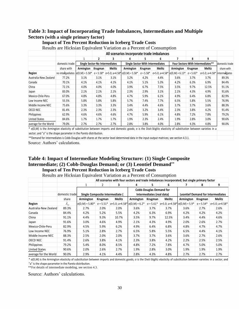
30

Table 3: Impact of Incorporating Trade Imbalances, Intermediates and Multiple

Sectors (with a single primary factor)

Impact of Ten Percent Reduction in Iceberg Trade Costs

Results are Hicksian Equivalent Variation as a Percent of Consumption

Source: Authors’ calculations.

Table 4: Impact of Intermediate Modeling Structure: (1) Single Composite

Intermediate; (2) Cobb-Douglas Demand; or (3) Leontief Demand**

Impact of Ten Percent Reduction in Iceberg Trade Costs

Results are Hicksian Equivalent Variation as a Percent of Consumption

**For details of intermediate modeling, see section 4.3.

Source: Authors’ calculations.

All scenarios incorporate trade imbalances1 2 3 4 5 6 7 8 9

domestic trade domestic trade

share with Armington Krugman Melitz Armington Krugman Melitz Armington Krugman Melitz share with

Region no intermediates σ(D,M) = 5.58* σ = 5.58* σ=5.0; a=4.58* σ(D,M) = 5.58* σ = 5.58* σ=5.0; a=4.58* σ(D,M) = 6.13* σ = 5.65* σ=5.0; a=4.58* intermediates

Australia-New Zealand 77.2% 3.1% 3.1% 3.1% 3.2% 4.2% 4.4% 3.6% 3.7% 3.7% 89.3%

Canada 70.1% 4.1% 4.1% 4.1% 4.1% 5.1% 5.3% 4.2% 6.3% 6.9% 84.4%

China 72.1% 4.0% 4.0% 4.0% 3.9% 6.7% 7.5% 3.5% 9.7% 12.5% 91.1%

Japan 83.0% 2.1% 2.1% 2.1% 2.3% 2.9% 3.1% 2.1% 4.3% 4.9% 91.6%

Mexico-Chile-Peru 67.0% 4.8% 4.8% 4.8% 4.7% 5.9% 6.1% 4.9% 6.4% 6.8% 82.9%

Low Income NEC 55.5% 5.8% 5.8% 5.8% 5.7% 7.4% 7.7% 6.5% 5.8% 5.5% 76.9%

Middle Income NEC 75.6% 3.3% 3.3% 3.3% 3.4% 4.4% 4.6% 3.7% 3.7% 3.6% 88.3%

OECD NEC 81.4% 2.3% 2.3% 2.3% 2.4% 3.2% 3.4% 2.3% 3.8% 4.2% 91.4%

Philippines 62.9% 4.6% 4.6% 4.6% 4.7% 5.9% 6.1% 4.8% 7.2% 7.8% 79.2%

United States 84.6% 1.7% 1.7% 1.7% 1.9% 2.3% 2.4% 1.9% 2.8% 3.0% 90.6%

average for the World 79.0% 2.7% 2.7% 2.7% 2.8% 3.8% 4.0% 2.8% 4.3% 4.8% 90.0%

**Demand for intermediates is Cobb-Douglas with shares at the sector level determined data in the input-output matrices; see section 4.3.1.

Single Sector-No Intermediates Single Sector-With Intermediates Four Sectors-With Intermediates**

* σ(D,M) is the Armington elasticity of substitution between imports and domestic goods; σ is the Dixit-Stiglitz elasticity of substitution between varieties in a

sector; and "a" is the shape parameter in the Pareto distribution.

rr rr

All scenarios with four sectors and trade imbalances incorporated; but single primary factor

1 2 3 4 5 6 7 8 9

domestic trade

share Armington Krugman Melitz Armington Krugman Melitz Armington Krugman Melitz

Region σ(D,M) = 5.80* σ = 5.51* σ=5.0; a=4.58* σ(D,M) = 6.2* σ = 5.61* σ=5.0; a=4.58* σ(D,M) = 5.9* σ = 5.54* σ=5.0; a=4.58*

Australia-New Zealand 89.3% 2.7% 2.0% 2.0% 3.6% 3.7% 3.7% 3.6% 2.7% 2.6%

Canada 84.4% 4.2% 5.2% 5.5% 4.2% 6.3% 6.9% 4.2% 4.2% 4.2%

China 91.1% 4.4% 9.3% 10.7% 3.5% 9.7% 12.5% 3.4% 4.4% 4.6%

Japan 91.6% 3.0% 4.6% 4.9% 2.1% 4.3% 4.9% 2.0% 2.6% 2.7%

Mexico-Chile-Peru 82.9% 4.5% 5.9% 6.2% 4.9% 6.4% 6.8% 4.8% 4.7% 4.7%

Low Income NEC 76.9% 5.1% 2.8% 2.7% 6.5% 5.8% 5.5% 6.5% 4.4% 4.1%

Middle Income NEC 88.3% 2.5% 2.0% 2.0% 3.7% 3.7% 3.6% 3.6% 2.7% 2.6%

OECD NEC 91.4% 2.6% 3.8% 4.1% 2.3% 3.8% 4.2% 2.2% 2.5% 2.5%

Philippines 79.2% 5.4% 8.0% 8.5% 4.8% 7.2% 7.8% 4.7% 5.0% 5.0%

United States 90.6% 2.0% 2.6% 2.7% 1.9% 2.8% 3.0% 1.9% 1.9% 1.9%

average for the World 90.0% 2.9% 4.1% 4.4% 2.8% 4.3% 4.8% 2.7% 2.7% 2.7%

* σ(D,M) is the Armington elasticity of substitution between imports and domestic goods; σ is the Dixit-Stiglitz elasticity of substitution between varieties in a sector; and

"a" is the shape parameter in the Pareto distribution.

Cobb-Douglas Demand for

Intermediates (real data) Leontief Demand for IntermediatesSingle Composite Intermediate (

rr