Comparison of Two Automated Methods for QT Interval Measurement

RE Gregg, S Babaeizadeh, DQ Feild, ED Helfenbein, JM Lindauer, SH Zhou

Advanced Algorithm Research Center, Philips Medical Systems, Andover, MA, USA

Abstract

In this paper we compared two methods of automated

QT interval measurement on standard ECG databases:

the Root-Mean-Square (RMS) lead combining method

aimed at QT monitoring and the method of median of

lead-by-lead QT interval measurements.

We used the PhysioNet PTB (N=548) and CSE

measurement (N=125) standard databases. Both have

reference QT interval measurements from a group of

annotators. The last 10 seconds of each PTB record was

downsampled from 1000 sample per second (sps) and an

amplitude resolution of 1 µV to 500 sps and 5 µV in order

to match the CSE set. PTB records #205 and #557 were

excluded due to ventricular paced rhythm and artifact,

respectively. Twenty five cases were excluded from the

CSE set to match the selection of cases for IEC algorithm

testing (IEC 60601-2-51).

We processed all records using the Philips resting 12-

lead ECG algorithm to generate representative beats for

QT interval measurement. The RMS method measures

QRS onset and end of T on an RMS waveform constructed

from 9 leads I, II, III and V1-V6. The lead-by-lead method

takes the median QT interval across leads. The automated

QT intervals by the RMS and lead-by-lead methods were

compared to the reference manual QT measurements.

The mean difference between the lead-by-lead QT and

the reference QT was 1.7±9.7ms and 12.4±23.0ms (mean

±standard deviation (SD)) for the CSE and PTB sets

respectively. For the RMS method, the mean difference

was -2.8±11.1ms and 10.3±20.9ms. F-tests indicate that

the standard deviation between methods is not

significantly different for the CSE set (P=0.18) or the

PTB set (P=0.77).

The lead-by-lead and RMS methods perform similarly,

leading to the conclusion that the choice between them

should be based on considerations such as the number of

leads available or computational efficiency.

1. Introduction

Global QT interval is one of the fundamental ECG

measurements reported on virtually every 12 lead ECG. A

longer than normal QT interval may indicate a congenital

or acquired long QT condition [1-3]. The AHA/ACC

practice guideline for ECG monitoring now includes a

recommendation to monitor QT interval for the purpose

of drug titration of drugs known to have a pro-arrhythmic

effect [4]. If the QT interval lengthens by more than 60ms

after starting the drug or the QT interval extends beyond

500 ms the administration of the drug should be stopped

or the dosage can be reduced.

We have previously presented Philips automated QT

interval measurement algorithms for 12-lead ECG, Holter

and ECG monitoring applications [5-10]. In the

ambulatory Holter and patient monitoring ECG

applications, the QT interval algorithm uses an RMS

waveform from combined available high quality leads

and measures QT interval on the RMS ECG. In the

resting 12-lead ECG application, the global QT interval

measurement is based on a lead-by-lead method. The

open question is, of the two, which method is better

ignoring the constraints of the application. In this paper,

we compared the two automated methods and reported

the results using the same ECG datasets.

2. Study Population

A comparison between automated methods aimed at

either monitoring or ambulatory ECG versus 12-lead

ECG is hampered by the gross difference in available

ECG in each case. Ambulatory ECGs cannot be used to

test the 12-lead QT algorithm because of low sample rate,

narrow bandwidth and limited leads. For 12-lead ECG

analysis, a sample rate of 500 sps and a bandwidth of 0.05

to 150Hz are required. Ambulatory ECG recordings often

have sample rates around 200 sps and a cut-off frequency

of 40Hz. Only selected parts of the 12-lead analysis are

possible with the small number of leads used in an

ambulatory or monitoring recording. On the other hand,

the sample rate, bandwidth and number of leads may be

adequate for a 12-lead ECG to be used for an ambulatory

analysis, but the 10 second recording is not long enough

for even the learning period of the ambulatory and

monitoring algorithms

The addition of the PTB set to the data publicly

available at PhysioNet made this study possible because it

has the features that allow direct comparison between

ambulatory and 12 lead algorithms [11]. The PTB dataset

consists of 549 records from 294 subjects with a sample

ISSN 0276−6574 427 Computers in Cardiology 2007;34:427−430.

rate of 1000sps, an amplitude resolution of 1uV, 12 scalar

and 3 vector leads. In our analysis, the last 10 seconds of

each record was down-sampled to a resolution of 500 sps

and 5 µV. Records #205 and #557 were excluded due to

ventricular pacing and heavy artefact respectively.

Reference manual QT intervals were collected from

multiple annotators as part of the Computers in

Cardiology 2006 challenge [12].

In general, automated ambulatory and 12 lead

algorithms can be compared at the representative beat

section of the algorithms. Most algorithms time-align and

average many like-morphology beats together and extract

features from that representative beat as discussed by

Willems et al [13]. Through measurements made on the

representative beat, results from longer ECG records and

short 10 second ECG records can be compared. A second

data set from the CSE project was used here [14]. The

100 ten-second records were selected from the total 125

according to the selection for computerized algorithm

testing in the essential performance standard IEC 60601-

2-51. Since the goal of the CSE and IEC effort was a

minimum standard of measurement accuracy, problem

cases such as atrial fibrillation were excluded because of

undefined measurements. The resolution of the CSE 10

second records was 500 sps and 5 µV per LSB.

3. Methods

The Philips resting 12-lead ECG algorithm was used to

process all PTB and CSE records to produce

representative beat signals. The dominant morphology

beats were time-aligned and averaged to produce the

representative beat. Custom MATLAB programs were

used for the remaining processing. Statistical analysis was

performed with the S-PLUS statistical software package.

In the lead-by-lead method of automated QT interval

measurement, the QRS onset and end of T wave are

determined separately. Although the earliest QRS onset

and last T end are desired, the best accuracy and

statistical stability is achieved using order statistics

somewhere between the median and the maximum or

minimum. Order statistics are a method of sorting a set of

values and choosing one value from the set by order in

the same way that the 50% value corresponds to the

median. In our case, the QRS onset and T end times

across leads I, II, III and V1-V6 are sorted. For global

QRS onset, the 33% value is chosen. The 50% value is

chosen for the global T end. The Philips method was also

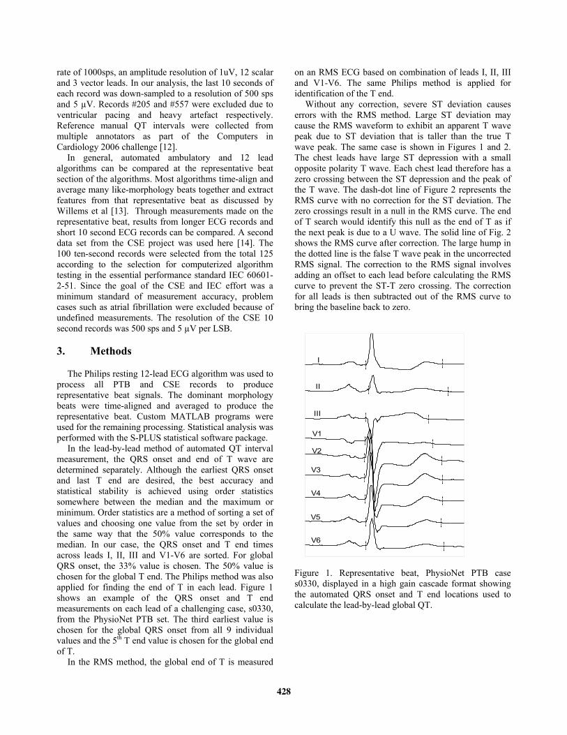
applied for finding the end of T in each lead. Figure 1

shows an example of the QRS onset and T end

measurements on each lead of a challenging case, s0330,

from the PhysioNet PTB set. The third earliest value is

chosen for the global QRS onset from all 9 individual

values and the 5th T end value is chosen for the global end

of T.

In the RMS method, the global end of T is measured

on an RMS ECG based on combination of leads I, II, III

and V1-V6. The same Philips method is applied for

identification of the T end.

Without any correction, severe ST deviation causes

errors with the RMS method. Large ST deviation may

cause the RMS waveform to exhibit an apparent T wave

peak due to ST deviation that is taller than the true T

wave peak. The same case is shown in Figures 1 and 2.

The chest leads have large ST depression with a small

opposite polarity T wave. Each chest lead therefore has a

zero crossing between the ST depression and the peak of

the T wave. The dash-dot line of Figure 2 represents the

RMS curve with no correction for the ST deviation. The

zero crossings result in a null in the RMS curve. The end

of T search would identify this null as the end of T as if

the next peak is due to a U wave. The solid line of Fig. 2

shows the RMS curve after correction. The large hump in

the dotted line is the false T wave peak in the uncorrected

RMS signal. The correction to the RMS signal involves

adding an offset to each lead before calculating the RMS

curve to prevent the ST-T zero crossing. The correction

for all leads is then subtracted out of the RMS curve to

bring the baseline back to zero.

I

II

III

V1

V2

V3

V4

V5

V6

Figure 1. Representative beat, PhysioNet PTB case

s0330, displayed in a high gain cascade format showing

the automated QRS onset and T end locations used to

calculate the lead-by-lead global QT.

428

400 500 600 700 800 900

0

100

200

300

400

500

600

time (ms)

RM

S/a

ctivity

Figure 2. RMS waveform (solid line) of the same ECG

signal as shown in Fig. 1. The uncorrected RMS

waveform in dotted-line is calculated by combining leads

I, II, III, and V1-V6. The dash-dotted line illustrates the

corresponding activity.

In the RMS method, QRS onset is determined from an

activity signal rather than the RMS signal. The activity

function is defined below by equation 1. It is the absolute

value first difference signal summed across leads. Since

the high frequency content of the QRS part of the

complex far exceeds the high frequency content of P and

especially T waves, the peaks of the QRS part of the

activity function are large compared to the rest of the

complex. Although the activity function is susceptible to

high frequency noise because of the use of first

differences, beat-averaging before the activity function

calculation and lowpass filtering of the activity function

reduce the noise susceptibility.

(1) ∑=

−−=

L

j

ixjxjiyi1

|)1(|

4. Results

The differences between automated measurement of

QT interval and the reference manual QT interval are

summarized below in Table 1. The differences between

automated and manual QT measurements are

characterized by mean difference (automated minus

manual), and the standard deviation.

Table 1. QT differences, automated minus manual, for the

two automated methods on both the CSE and PTB sets.

SD = standard deviation.

Automated

algorithm

CSE

(N=100)

PTB

(N=546)

Mean

(ms)

SD

(ms)

Mean

(ms)

SD

(ms)

Lead-by-lead 1.7 9.7 12.4 23.0

RMS -2.8 11.1 10.3 20.9

The striking feature of the test results is the similarity

of standard deviation of QT measurement differences and

the approximate 3 ms mean difference between the

methods on the two data sets. The F-test indicate that the

difference in standard deviation between the methods is

not significant for the CSE set (p=0.18) or the PTB set

(p=0.77). For the CSE set, the paired T-test results in a

difference of 4.5 ms between methods with a 95%

confidence interval of 1.7 to 7.3 ms. For PTB, the

difference between automated methods is 2.0 ms with a

confidence interval of 0.2 to 3.9 ms.

The median and interquartile range (IQR) are used to

measure the central tendency and variation in QT interval

differences without undue effect of outliers. The median

and IQR values in Table 2 show a similar result as mean

and standard deviation. The lead-by-lead method has

slightly less variation for the CSE set and the RMS

method has slightly less variation for the PTB set. The

difference between median values is close to the

difference in means.

Table 2. Median and interquartile range (IQR) of QT

differences for CSE and PTB sets.

Automated

algorithm

CSE

(N=100)

PTB

(N=546)

Median

(ms)

IQR

(ms)

Median

(ms)

IQR

(ms)

Lead-by-lead 1.0 9.5 11.0 19.5

RMS -3.0 12.3 9.0 19.0

5. Discussion

The mean difference between methods has a somewhat

consistent small bias of approximately 3ms for both data

sets according to the paired T-tests. Both methods are

close to zero mean performance for the CSE set while

both methods measure QT long by approximately 10ms

compared to the manual annotation for the PTB set. This

suggests a potential bias in the reference QT

measurements between the CSE and PTB sets. Bortolan

trained on the CSE and tested on the PTB set and also

reported a bias in reference QT measurements with a

much larger value of 25 ms [13]. This bias could easily be

explained by the fact that the PTB annotators

concentrated on lead II while the CSE annotators used 8

available leads I, II and V1 – V6 [14,15].

From the results in Table 1 and Table 2, it is difficult

to choose one automated method over the other since

each method is slightly better for one of the two sets but

not both. The lead-by-lead method results in better on-

target performance and low variation for the CSE set

while the RMS method has a smaller mean difference and

measurement variation on the PTB set. Each data set has

429

advantages and disadvantages. The CSE group collected

ECGs to represent a general hospital population. The PTB

patient selection is composed of a high proportion of

myocardial infarction (MI) cases and a smaller group of

normal subjects. The CSE set was annotated on multiple

leads by multiple annotators very carefully and the

method was well documented [16]. All primary leads

were used and the annotation was performed on high

resolution ECG which has been shown to affect the QT

measurement [17]. The annotators of the PTB database

were instructed to concentrate on only lead II. On the

other hand, the PTB set has 550 cases compared to the

CSE set of 125 cases. The effect of larger population can

be seen in the tight confidence interval for the mean QT

difference for the PTB set. Since the CSE set was

annotated across all leads at a high gain, we weigh the

CSE results more heavily and therefore believe our

automated methods to be on-target even though they

exhibit a 10 ms bias according to the PTB set.

6. Conclusion

In conclusion, the two automated methods presented

produce comparable results so that either method could

be chosen. Both methods perform well. The lead-by-lead

method requires more leads for the application of order

statistics to make sense. The RMS method can use just a

single lead. For this reason, both the lead-by-lead and

RMS methods can be used for 12 lead resting ECG

analyses. However, the lead-by-lead method does require

more computational power. In real-time monitoring and

ambulatory ECG applications with a limited number of

leads available and restrained computational power, the

RMS method works well and should be used.

References

[1] Moss A. QTc prolongation and sudden cardiac death. JACC

2006;47:2:368-369.

[2] Towbin J, Friedman R. Prolongation of the QT interval and

the sudden infant death syndrome. N Engl J Med

1998;338:1760-1761.

[3] Priori SG, Schwartz PJ, Napolitano C, et al. Risk

stratification in the long-QT syndrome. N Engl J Med

2003;348:1866-1874.

[4] Drew BJ, Califf RM, Funk M, et. al. Practice standard for

Electrocardiographic monitoring in hospital settings. An

American Heart Association Scientific Statement from the

councils on cardiovascular nursing, clinical cardiology and

cardiovascular disease in the young. Circulation

2004,110:2721-2746.

[5] Lindauer JM, Gregg RE, Helfenbein ED, Shao M, Zhou SH.

Global QT measurements in the Philips 12-lead algorithm. J

Electrocardiol, 2005, Vol. 38: p S90.

[6] Feild DQ, QT measurement performance in a Holter

application. J Electrocardiol 2005, 38:S34.

[7] Helfenbein ED, Zhou SH, Lindauer JM, Feild DQ, Gregg

RE, Wang JY, Kresge SS, Michaud FP. An algorithm for

continuous real-time QT interval monitoring. J

Electrocardio 2006;39:S123-S127.

[8] Helfenbein ED, Zhou SH, Feild DQ, Lindauer JM, Gregg

RE, Wang JY, Kresge SS, Michaud FP. Performance of a

continuous real-time QT interval monitoring algorithm for

the critical-care setting. Computers in Cardiology 2006,

33:697-700.

[9] Helfenbein ED, Ackerman MJ, Rautaharju PM, Zhou SH,

Gregg RE et al.: An algorithm for QT interval monitoring

in neonatal intensive-care units. J Electrocardiol 2007

(supp) (in press)

[10] Zhou SH, Helfenbein ED, Lindauer JM, Gregg RE, Feild

DQ: Philips QT interval measurement algorithms for

diagnostic, ambulatory and patient monitoring ECG

applications. ANE, 2007 suppl. (in press)

[11] Goldberger AL, Amaral LAN, Glass L, Hausdorff JM,

Ivanov PCh, Mark RG, Mietus JE, Moody GB, Peng CK,

Stanley HE. PhysioBank, PhysioToolkit, and PhysioNet:

Components of a New Research Resource for Complex

Physiologic Signals. Circulation 2000, 23:e215-e220.

[12] Moody GB, Koch H, Steinhoff U. The

PhysioNet/Computers in Cardiology Challenge 2006: QT

interval measurement. Computers in Cardiology (33) 2006.

[13] Bortolan G. Algorithmic testing for QT interval

measurement. Computers in Cardiology 2006, 33:365-368.

[14] Willems JL, Arnaud P, van Bemmel JH, Bourdillon PJ,

Degaini R, et al. Establishment of a reference library for

evaluating computer ECG measurement programs. Comput.

Biomed Research 1985, 18:439-457.

[15] Willems JL, Arnaud P, van Bemmel JH, Degani R,

Macfarlance PW, Zywietz C. Common standards for

quantitative electrrcardiography: goals and main results.

Methods of Information in Medicine 1990, 29:263-271.

[16] Commission of the European Communities, Medical and

Public Health Research (Willems JL CSE Project Leader):

Common Standards for Quantitative Electrocardiography,

CSE Multilead Atlas. CSE Ref. 88-04.15 Acco Publ,

Leuven Belgia, 1988.

[17] Murray A, McLaughlin NB, Bourke JP, Doig JC, Furniss

SS, Campbell RWF. Errors in manual measurement of QT

intervals, Br Heart J 1994, 71:386-390.

Address for correspondence.

Richard Gregg

Advanced Algorithm Research Center (AARC)

Philips Medical Systems

3000 Minuteman Drive, Mail stop 0220

Andover, MA 01810

USA

rich.gregg@philips.com

430