IN DEGREE PROJECT COMPUTER SCIENCE AND ENGINEERING,SECOND CYCLE, 30 CREDITS

, STOCKHOLM SWEDEN 2020

Comparison of Player Tracking-by-Detection Algorithms in Football Videos

SUPING SHI

KTH ROYAL INSTITUTE OF TECHNOLOGYSCHOOL OF ELECTRICAL ENGINEERING AND COMPUTER SCIENCE

Comparison of PlayerTracking-by-DetectionAlgorithms in Football Videos

SUPING SHI

DA223X, Master’s Thesis in Computer Science (30 ECTS credits)Date: October 14, 2020Supervisor: Mårten Björkman, Volodya GrancharovExaminer: Danica Kragic JensfeltHost company: Ericsson ABSwedish title: En jämförelse av spårningsalgoritmer för spelare ifotbollsvideorSchool of Electrical Engineering and Computer Science

Abstract

In recent years, increasing demands on sports analytics have triggered growingresearch interest in automatic player tracking-by-detection approaches. Twoprominent branches in this area are Convolutional Neural Network (CNN)-basedvisual object detectors and histogram-based detectors.

In this thesis, we focus on a particular sub-domain: player tracking by de-tection in broadcast football games. To tackle challenges in this domain, suchas motion blur and varied image quality, two different systems are proposedbased on histogram and CNN respectively. With the help of transfer learning,the CNN-based system is fine-tuned from a pre-trained Tiny-You Only LookOnce (YOLO)-V2 model. Experiments are conducted to evaluate the CNN-based system against the histogram-based system and off-the-shelf benchmarks,such as Faster Region-based convolutional Neural Networks (R-CNN). Resultsindicate that the CNN-based system outperforms the others in terms of meanIntersection Over Union (IOU) and Mean Average Precision (mAP).

Furthermore, we combine the CNN-based system with a histogram-basedpost-processor to take advantage of the player’s visual appearance characteristic.The combined system is evaluated against the pure CNN-based system andCNN-Simple Online and Realtime Tracking (SORT) system. Results reveal thatthe combined system manages to achieve better detection accuracy in terms ofF1 and ITP scores.

1

Sammanfattning

Under de senaste aren har okande krav pa sportanalyser resulterat i ett vaxandeforskningsintresse for automatisk spelarsparning. Tva viktiga metoder inomdetta omrade ar CNN-baserade visuella objektdetektorer och histogrambaseradedetektorer.

I rapporten fokuserar vi pa ett visst underomrade, namligen spelarsparninggenom detektion i direktsandning av fotbollsmatcher. For att hantera ut-maningar som rorelseoskarpa och varierande bildkvalitet, foreslas tva olika sys-tem baserade pa histogram respektive CNN. Med hjalp av overforingsinlarningfinjusteras det CNN-baserade systemet med utgangspunkt i en fortranad Tiny-YOLO-V2 modell. Experiment genomfors for att utvardera det CNN-baseradesystemet mot det histogrambaserade systemet och standardlosningar som R-CNN. Resultaten indikerar att det CNN-baserade systemet ger battre resultatvad galler medelvarden som IOU och mAP.

Dessutom kombinerar vi det CNN-baserade systemet med en histogram-baserad postprocessor for att ocksa anvanda oss av spelarens visuella karak-teristika. Det kombinerade systemet utvarderas mot det rena CNN-baseradesystemet och CNN-SORT systemet. Resultaten visar att det kombinerade sys-temet lyckas uppna battre detektionsnoggrannhet nar det galler F1 och ITPpoang.

Acknowledgment

Firstly, I would like to thank my supervisors Volodya Grancharovat in EricssonResearch for his great advices and prompt feedback on this project. I wouldalso appreciate Sigurdur Sverrisson in Ericsson research for knowledge sharingand Harald Plboth for his line support and keen interest in this topic.

Secondly, I want to express my gratitude to my academic supervisor MartenBjorkman from KTH for all the good technical discussions and suggestions onthe writing of this thesis.

Lastly, I would like to appreciate my beloved husband and parents, who giveme consistent supports during my study.

Contents

1 Introduction 61.1 Background . . . . . . . . . . . . . . . . . . . . . . . . . . . . . . 61.2 Ethical Problems and Social Implications . . . . . . . . . . . . . 71.3 Research Questions . . . . . . . . . . . . . . . . . . . . . . . . . . 81.4 Thesis Organization . . . . . . . . . . . . . . . . . . . . . . . . . 8

2 Methodology and Related Works 92.1 Multi-Object Tracking . . . . . . . . . . . . . . . . . . . . . . . . 9

2.1.1 Tracking by Detection . . . . . . . . . . . . . . . . . . . . 92.1.2 Pioneering Work on Player Detection and Tracking . . . . 10

2.2 Visual Object Detectors in Sports Videos . . . . . . . . . . . . . 112.3 CNN-based Visual Object Detectors . . . . . . . . . . . . . . . . 11

2.3.1 Overview of the Field . . . . . . . . . . . . . . . . . . . . 112.3.2 Faster R-CNN . . . . . . . . . . . . . . . . . . . . . . . . 122.3.3 YOLO . . . . . . . . . . . . . . . . . . . . . . . . . . . . . 142.3.4 Single Shot MultiBox Detector . . . . . . . . . . . . . . . 162.3.5 Transfer Learning . . . . . . . . . . . . . . . . . . . . . . 16

2.4 Histogram-based Detectors . . . . . . . . . . . . . . . . . . . . . 172.4.1 Color Space . . . . . . . . . . . . . . . . . . . . . . . . . . 172.4.2 Color Histogram Distribution . . . . . . . . . . . . . . . . 182.4.3 Metric for Histogram Distance . . . . . . . . . . . . . . . 18

3 Methods 203.1 Dataset . . . . . . . . . . . . . . . . . . . . . . . . . . . . . . . . 20

3.1.1 Training Sequences . . . . . . . . . . . . . . . . . . . . . . 203.1.2 Testing Sequences . . . . . . . . . . . . . . . . . . . . . . 22

3.2 Color Histogram-based System . . . . . . . . . . . . . . . . . . . 243.2.1 Color Histogram Distribution . . . . . . . . . . . . . . . . 253.2.2 Evaluation of Similarity . . . . . . . . . . . . . . . . . . . 25

3.3 CNN-based System . . . . . . . . . . . . . . . . . . . . . . . . . . 273.3.1 Network Architecture of CNN . . . . . . . . . . . . . . . . 273.3.2 Training . . . . . . . . . . . . . . . . . . . . . . . . . . . . 29

3.4 Combined System . . . . . . . . . . . . . . . . . . . . . . . . . . 293.4.1 Histogram-based Post Processor . . . . . . . . . . . . . . 293.4.2 Workflow . . . . . . . . . . . . . . . . . . . . . . . . . . . 32

3.5 Evaluation . . . . . . . . . . . . . . . . . . . . . . . . . . . . . . . 343.5.1 Evaluation Metrics . . . . . . . . . . . . . . . . . . . . . . 35

2

4 Experiment Results 364.1 Histogram-based System . . . . . . . . . . . . . . . . . . . . . . . 36

4.1.1 Positive Detections . . . . . . . . . . . . . . . . . . . . . . 364.1.2 Negative Detections . . . . . . . . . . . . . . . . . . . . . 37

4.2 CNN-based System . . . . . . . . . . . . . . . . . . . . . . . . . . 374.2.1 Comparison between CNN-based System and Histogram-

based System . . . . . . . . . . . . . . . . . . . . . . . . . 394.2.2 Comparison between CNN-based System and Off-the-shelf

Systems . . . . . . . . . . . . . . . . . . . . . . . . . . . . 404.3 Combined System . . . . . . . . . . . . . . . . . . . . . . . . . . 43

4.3.1 Evaluation of Tracking Performance . . . . . . . . . . . . 43

5 Discussion and Conclusions 445.1 Limitations . . . . . . . . . . . . . . . . . . . . . . . . . . . . . . 44

5.1.1 Dataset . . . . . . . . . . . . . . . . . . . . . . . . . . . . 445.1.2 YOLO . . . . . . . . . . . . . . . . . . . . . . . . . . . . . 455.1.3 Histogram-based System . . . . . . . . . . . . . . . . . . . 45

5.2 Conclusions . . . . . . . . . . . . . . . . . . . . . . . . . . . . . . 465.2.1 Future Work . . . . . . . . . . . . . . . . . . . . . . . . . 47

3

Glossary

ANN Artificial Neural Network. 11

CNN Convolutional Neural Network. 1, 2, 3, 7, 8, 10, 11, 12, 17, 20, 27, 28,29, 32, 33, 34, 37, 39, 40, 41, 42, 43, 45, 46, 47

COCO Common Objects in COntext. 16

DPM Deformable Parts Model. 11, 14

GPU Graphics Processing Unit. 29

HOG Histogram of Oriented Gradient. 11, 18

HSI Hue-Saturation-Intensity. 17

HSV Hue-Saturation-Value model. 17, 18

ILSVRC ImageNet Large Scale Visual Recognition Challenge. 16

IOU Intersection Over Union. 1, 15, 35, 39, 46

ITP Identity Tracking Performance. 35

LAB LAB color space. 17

mAP Mean Average Precision. 1, 42, 46

PASCAL Pattern Analysis, Statical Modeling and Computational Learning.13, 16

R-CNN Region-based convolutional Neural Networks. 1, 2, 8, 11, 12, 13, 14,16, 22, 34, 40, 42, 43, 46

RGB Red-Green-Blue model. 17, 18, 25

RPN Region Proposal Network. 13, 14

SIFT Scale Invariant Feature Transform. 11

SORT Simple Online and Realtime Tracking. 1, 7, 34, 43, 46

4

SSD Single Shot MultiBox Detector. 16

SVM Support Vector Machine. 12

VOC Visual Object Classes. 13, 16

YOLO You Only Look Once. 1, 2, 3, 11, 14, 15, 16, 17, 22, 34, 40, 41, 42, 45,46

YUV YUV color space. 17

5

Chapter 1

Introduction

1.1 Background

In the past few decades, football has become one of the most popular sportsthat millions of people enjoy. With the expansion of internet and new mediatechnologies, football analytics has gained growing attentions and demands fromfootball clubs and players. One of the top requirements for football analyticsis to get tracking information of players in football games, which will supportcoaches and sports scientists to prepare attack and defense strategy for futuregames. Also, players may have a need for such information to review and im-prove their performance during training or official games. To serve this demand,new methods for football analytics are proposed and developed by researcherson a daily basis. Detection and tracking of players in a football game are twoessential parts within this area.

It has been a challenge for a long time to automatically detect and trackplayers across a scene in video streams. Requirements on the quality of footballanalytics demand that the accuracy of player detection and tracking approachesneeds to be guaranteed. There are several factors that may pose a negativeinfluence on the performance of player detection and tracking in football games:

• Motion blur: Players in the videos of football games usually move withhigh speed and may appear blurry in the image.

• Complex motion pattern: Players usually have much more human posturepatterns than normal pedestrians.

• Severe occlusion between the multiple players of interest.

Due to these reasons, player detection and tracking in broadcast footballvideos is a particularly challenging task in computer vision area. One of theprominent methods to tackle this task is background subtraction. The modellingof background subtraction contains two steps:

• The initialization of the background.

• The update of the background.

6

Background subtraction normally performs better with a static camera thana moving one. The changing of the background may have a negative impacton the detection performance. Template matching is also widely used in sportsgraphics systems. In the paper [1], the American football players are tracked bytemplate matching and Kalman filtering. Tracking-by-detection has come intoour view in recent years. The detection algorithm is continuously applied oneach frame of a video sequence to generate region proposals of players. Thenthe association of detections between consecutive frames are involved in thetracking-by-detection method.

Nowadays, the attention is rising rapidly on applying CNN as a detector inthe tracking-by-detection method, since it can achieve a significantly fast speedand high accuracy when dealing with visual recognition tasks. In the paper[2], the authors proposed a CNN-based detector, namely SORT, for multipleobject tracking. It mainly focuses on frame-to-frame associations of objects foronline and real time applications. The authors approximated the inter-framedisplacements of each object with a linear constant velocity model.

The tracking-by-detection area has recently attracted interest from the re-search community and sports analytic companies. As one of such organizations,the Piero sports team aims to build an autonomous system to produce playerdetections in broadcast football videos. The objective of this thesis is to developdifferent tracking-by-detecting algorithms in football games and compare themwith benchmarks.

1.2 Ethical Problems and Social Implications

This thesis proposes several systems for player tracking-by-detection in footballvideos and strives to benchmark the performances of the proposed systems onbroadcast football video sequences. The outcome of this work would be compar-ative results of the proposed systems for player tracking-by-detection in footballgames. Companies with relevant interests can reference to this work and expectvaluable information depending on their requirements.

The research of this topic requires a certain amount of training data tostudy players’ characteristics in football games. As we have entered the age ofdata, ethical considerations on data collection and usage should be well taken.Our work requires a large scale of data analysis in football videos, which mayexpose us to an ethical problem regarding data privacy. As Jules and Tenementioned in [3]: Big data poses big privacy risks. The harvesting of largesets of personal data and the use of state-of-the-art analysis implicates growingprivacy concerns. The data used for training and testing our neural networks ispublic football game videos provided and authorized by the Piero team. Beforenetwork training and testing, we manually draw bounding boxes and overlaythem on top of players. Though we do not get the authorization from eachplayer whose image is used in this experiment, the authorization for using thevideo sequences of the games is granted. Nowadays, videos of football gamesare widely used for analyzing a team or a player. As is noted in [4]: Researchersare legally obliged to conform with legal regulation relating to their research.Though ethics problems are not equivalent to legal problems, we still shouldtake them carefully and seriously. To avoid ethical issues and respect people’sprivacy, our data would not be transferred to any other parties for other usages.

7

1.3 Research Questions

This work is conducted under the supervision of Ericsson Research team inEricsson AB. The video clips are provided by the Piero team [5], and the col-lection of football videos should not be managed by this thesis. This paper firstpresents two base algorithms for tracking-by-detection of players in real-timefootball videos, and then compares them performance-wise with conventionalbenchmarks. The idea of combining the two base systems to take advantage ofboth algorithms is also investigated and evaluated. The major research ques-tions in this thesis can thus be formulated as follows:

1. How are the performances of the histogram-based system and CNN-basedsystem? Which one performs better on our real-time testing sequences?

2. How is the performance of the CNN-based system compared to the off-the-shelf systems, such as Faster R-CNN? What contributes to the successor failure of this proposed system?

3. How is the performance of the combined system? What contributes to thesuccess or failure of this proposed system?

1.4 Thesis Organization

This thesis is divided into individual chapters and organized as follows.Chapter 1 provides a brief introduction of the background. Ethical problems

and social implications are discussed in this chapter and followed by researchquestions.

The methodology and related research works are discussed and illustratedin Chapter 2. Previous research works for multi-object tracking, such as CNNand histogram-based detectors, are walked through in this chapter.

In Chapter 3, detailed explanations of the proposed systems are demon-strated, as well as the preparation of dataset for training and testing. Theevaluation of the proposed systems are also included in this chapter.

Chapter 4 demonstrates and interprets the experiment results for each pro-posed system.

Chapter 5 structures a discussion about potential limitations of the results.The thesis is concluded with answers to the research questions and future work.

8

Chapter 2

Methodology and RelatedWorks

2.1 Multi-Object Tracking

When it comes to computer vision, the first thing that comes into our mindswould be image classification. Classification is one of the fundamental tasks incomputer vision area. Though we can use a classification method to recognize anobject, it fails to provide us with the position information. Due to the academicand commercial potentials, methods for object detection has gained increasingpopularity. In 2001, an efficient algorithm for face detection was developed byPaul Viola and Michael Jones in [6]. The algorithm is fast enough to performface detection in real-time videos. New methods for object detection have beenconsistently introduced since then and triggered numerous innovative ideas inrelated areas.

Multi-object tracking is one of the most popular topics nowadays within thetracking area. It is hugely required in diverse areas and scenarios, such as sportsanalytics and self-driving cars. Sports players, pedestrians or vehicles can all beregarded as the objects to be tracked. The objective of multi-object tracking isto locate multiple targets in consecutive video frames and label their identities.When narrowed down to sports video scenarios, multi-object tracking is facedwith several challenges. As presented in the paper [7], though people haveproposed several methods to tackle this problem, these methods still suffer fromdifficulties, such as object occlusions and close similarity of multiple objects.One of the key publications in sports tracking [8] proposed an approach to solvethe problem of labeling the identities by using track graphs to track isolatedobjects. In this way, the identity in each track graph can be well maintained.The paper defined a similarity metric for each isolated track graph. By doingso, the identities of the isolated tracks can be associated easily.

2.1.1 Tracking by Detection

As the name indicates, tracking by detection aims to achieve object trackingby continuously applying a detection algorithm to consecutive frames of a videosequence. The generated detections in a given frame are then associated with

9

those in the previous frame. Methods for association of detections across framesis studied in these papers [9–12].

Tracking

In the simplest form, tracking is mainly defined as estimating the trajectoryof an object as it moves in a video or a moving scene. In object tracking, thedetection model and the tracking strategy are two key components. There areplenty of tracking strategies that can be applied for object tracking, such asKalman filter [13] and Particle filter [14].

Visual Object Detectors

The detection model plays an important role in the detection-based tracking.With the fast development of object tracking research, various types of detectionmodels have been proposed for object tracking in the previous works, such asfeature points [15], color [15–20], templates [15, 21–23] , and moving areas [24].The best-known detectors before the emergence of CNN model are Viola andJones’s algorithm proposed in [25] and the deformable part models proposed in[26]. The paper [25] described a machine learning approach for visual objectdetection. It introduced a new image representation called ’integral image’ toaccelerate the computation process. A learning algorithm based on Adaboostwas then applied in the paper. [26] proposed a detection system using a mixtureof multiscale deformable part models. Instead of using one model for objecttracking, the detection model in [26] utilized a root filter together with partfilters so that it could represent highly variable object classes.

Recently, the development in the area of object detection has contributedan increasing amount of promising detection models. Various object detectorsprovide a diverse source of detection models for tracking-by-detection tasks. Forexample, face detectors were applied for player tracking and evaluated positively,as shown in the paper [19].

2.1.2 Pioneering Work on Player Detection and Tracking

Even though multi-target tracking is widely developed and utilized for sportsgame analysis, it is still faced with challenges and has to cope with the factthat players typically move fast and adopt unusual postures when competing insports games. In [27] and [1], a pipeline was proposed to solve this task: Playerswere first segmented and filtered out from each video frame. The backgroundwas assumed to have a uniform color. Then the filtered players were tracked bytemplate matching and Kalman filter. In [27], teams of players were identifiedon the basis of color distributions. In this way, they first created a binary imagerepresentation based on the distance to the mean color of the background. Thenthey applied a threshold to the distance based on 3 standard deviations. In orderto remove small errors, erosion and dilation were applied to the binary imagerepresentation.

10

2.2 Visual Object Detectors in Sports Videos

As mentioned above, tracking players in a sports game is challenging due tothe fact that players usually have more postures than regular pedestrians. Thespeed of players is usually faster than that of pedestrians as well. Besides,occlusions of players happen frequently during sports games. All these issuesadd up to the difficulties in applying visual object detectors for player tracking.

As we mentioned before, Viola and Jones’s algorithm in [25] and DeformableParts Model (DPM) proposed in [28] are the best-known detectors before theemergence of CNN model. In the paper [16], the authors implemented a pipelineto detect and track players in hockey games based on Viola and Jones’s algo-rithm. In order to adapt the detection model to track players, the paper [28]proposed a deformable parts model instead of treating the detection model as awhole. Since players usually have more complicated postures than pedestrians,the deformable parts model is adequate to capture each part of these posturesand model players when putting the posture detections together.

The visual object detectors are usually far from perfection. The main prob-lems of detection-based object tracking algorithms are poor detection precisionand false positives. As a solution to mitigate these problems, methods in [29]and [17] fused multiple cues concurrently. In the paper [17], a weighted mask wasapplied to focus the descriptor vector on the team uniform’s area in a boundingbox. This practice guarantees that the upper-middle region of the boundingbox is mainly considered, around which the uniform is expected to appear witha higher possibility.

Recently, CNN-based detectors has achieved extraordinary success in thesports analytic area. The paper [2] proposed an efficient algorithm to achieveonline and real-time applications for object tracking. One similar applicationof CNN-based detectors in tracking-by-detection tasks in sports videos can befound in [30]. It followed the scheme proposed in [2] but replaced the FasterR-CNN with a YOLO-based detector. They proposed an online multi-detectionand tracking framework and performed experiments on a basketball dataset forevaluation.

2.3 CNN-based Visual Object Detectors

For a number of years, object recognition and detection in computer vision havebeen relying on color histograms or hand-designed features, such as Scale In-variant Feature Transform (SIFT) and Histogram of Oriented Gradient (HOG).However, these approaches only work well with low-level image details but fallshort in high-level information. Motivated by the recent success of deep learn-ing on object detection and recognition, we propose a CNN-based system inthis thesis and compare it with a variety of mature CNN architectures. In thissection, a brief introduction of relevant CNN-based visual object detectors arecovered as follows.

2.3.1 Overview of the Field

Artificial Neural Network (ANN) is a family of models inspired by human brains.It can learn how to represent complex non-linear relations between inputs and

11

outputs. The structure of a neural network is constructed with interconnectedneurons. The neurons are connected with links, which have associated weights.Typically, a neural network is composed of an input layer, several hidden layers,and an output layer. The hidden layers can be more than one. It is typicallyconsidered that the more hidden layers a neural network is composed of, thebetter it is capable of performing complex tasks. Similar findings can be foundin neuroscience that when a brain is processing information, it will go througha stacked architecture of hierarchically organized layers. Each layer can containnumerous neurons. The inputs of a neuron in a hidden layer come from all theneurons in the previous layer. The weighted sum of these inputs are calculatedand added with a bias term. Then this output value is passed to the next hiddenlayer after a non-linear activation function. When it has gone through all thehidden layers, the derived output is eventually returned to the output layer.

The application of neural networks as visual object detectors has enabledcomputers to detect multiple classes of objects with high accuracy, such as faces,pedestrians, and vehicles. However, neural networks usually suffer from a majordrawback: they require a large amount of labeled data for supervised learning.In order to solve this problem, [31] proposed a semi-supervised machine learningmethod to exploit both labeled and unlabeled data to train a classifier in anefficient way.

As is said in [32], CNN is a specific type of artificial neural networks thatutilizes convolution instead of vector operation. In the structure of CNN, con-volutional layers play a crucial role in extracting and detecting features fromimages. LeNet is known as the first prototype of CNN, which includes 3 con-volutional layers and one fully-connected layer. This network was proposed inthe paper [33] for dealing with the handwriting recognition task. Experimentresults demonstrated that LeNet outperformed all the other benchmarks backin the day.

2.3.2 Faster R-CNN

Recently, the class of R-CNN approaches have become fairly popular when deal-ing with object detection problems. One famous example of such type of meth-ods is R-CNN in [34].

Figure 2.1: Regions with CNN features [34].

This paper combined region proposals with a CNN model. As illustrated inFigure 2.1, the authors utilized a selective search algorithm to generate around2000 bottom-up region proposals. Each region proposal was fed into the CNNmodel to compute features. After that, they used a Support Vector Machine

12

(SVM) to classify each proposal. Experiment results have shown that throughR-CNN, the mean average precision can reach 53.7% on the test data set PatternAnalysis, Statical Modeling and Computational Learning (PASCAL) Visual Ob-ject Classes (VOC) 2010. However, the computational cost is hugely expensivefor R-CNNs, as mentioned in this paper [34]. One year later, Ross Girshick em-ployed several innovations for the previous work R-CNN to improve the speed oftraining and testing. The improved framework was referred to as Fast R-CNNin [35].

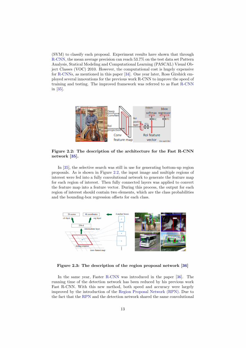
Figure 2.2: The description of the architecture for the Fast R-CNNnetwork [35].

In [35], the selective search was still in use for generating bottom-up regionproposals. As is shown in Figure 2.2, the input image and multiple regions ofinterest were fed into a fully convolutional network to generate the feature mapfor each region of interest. Then fully connected layers was applied to convertthe feature map into a feature vector. During this process, the output for eachregion of interest should contain two elements, which are the class probabilitiesand the bounding-box regression offsets for each class.

Figure 2.3: The description of the region proposal network [36]

In the same year, Faster R-CNN was introduced in the paper [36]. Therunning time of the detection network has been reduced by his previous workFast R-CNN. With this new method, both speed and accuracy were largelyimproved by the introduction of the Region Proposal Network (RPN). Due tothe fact that the RPN and the detection network shared the same convolutional

13

features, the computational cost for generating region proposals was significantlyreduced. For the RPN, the inputs are a collection of full images regardless oftheir size, and the outputs are a group of anchor boxes, which are a set ofrectangular object proposals as described in the paper [36]. As is illustrated inthe Figure 2.3, the region proposals are generated when a small network is slidover the convolutional feature map output, which happens in the last sharedconvolutional layer. The outputs will pass through two fully connected layers.One of the fully connected layers is for the regression of the anchor boxes, andthe other one is for the classification of these boxes. The final output of theRPN are the objects’ bounding boxes and the predicted probability scores ofbeing an object.

Compared to the R-CNN and Fast R-CNN, Faster R-CNN employs an RPNinstead of the selective search to generate region proposals efficiently. Sincethe RPN and the detection network share the same convolutional features, thecomputational cost for generating region proposals is dramatically reduced.

2.3.3 YOLO

The above prior detection systems, such as R-CNN and Fast R-CNN, would firstuse region proposal methods to generate potential bounding boxes. Then theywould run classifiers on each region proposal to generate a probability score ofbeing an object. The regions with high scores will be filtered out and consideredas detections.

The algorithm YOLO proposed in the paper [37] performed detection basedon a different strategy. Instead of using complex pipelines, YOLO strives toachieve object detection by solving a regression problem. YOLO takes full im-ages as inputs and could derive final region proposals and object classes withpredicted probabilities through solely one stage. Therefore, it does not requirethe sliding window in DPM or the region proposal-based techniques in R-CNNsto separate the background and players first. Since YOLO can access the entireimages no matter during training or testing, it is capable of utterly understand-ing and capturing the contextual information for each class.YOLO is developedbased on the GoogLeNet [38]. As is shown in Figure 2.4, YOLO network con-tains 24 convolutional layers and 2 fully connected layers [37] in total.

Figure 2.4: The architecture of YOLO [37]

14

As shown in Figure 2.5, an input image is first divided into S × S grid cellsin YOLO. Then bounding boxes are predicted for each grid cell. The paper [37]sets the number of bounding boxes for each grid cell to be B and the numberfor class probabilities to be C. These predictions are eventually encoded andreturned as S × S × (B × 5 + C) tensors.

Figure 2.5: YOLO models detection as a regression problem. It di-vides an input image into S×S grid cells and for each grid cell predictsB bounding boxes [37].

Each bounding box in outputs contains not only its position, height andwidth but also the class information and the objectness confidence value. Asstated in [37], the objectness confidence value represents the probability of con-taining an object of any class, and the method for calculating such a value isexpressed in equation 2.1. If an object falls into the grid cell, then Pr(object)will be set to 1. Otherwise, it will take 0 as its value. IOU truth

pred denotes theIOU value between the predicted bounding box and the ground truth.

Confidence = Pr(object) · IOU truthpred (2.1)

Each grid cell also predicts a conditional class probability Pr(Classi|Object),which indicates the likelihood of the detected object belongs to Classi given thatthe grid cell contains an object. Then the class-specific confidence score for eachbounding box can be calculated based on equation 2.2.

Pr(Classi, Object) · IOU truthpred = Pr(Classi|Object) · Pr(Object) · IOU truth

pred

(2.2)The class-specific confidence score directly reflects the likelihood of a bound-

ing box containing an object from a given class. After obtaining this confidence

15

score for each bounding box, we can set a threshold to filter these boxes andapply non-max suppression to reduce repetitive detections. The major stepsof YOLO can be concluded as firstly resizing input images, secondly feedingimages into a single convolutional network, and thirdly thresholding the deriveddetections, as shown in Figure 2.6.

Figure 2.6: The main steps of the YOLO [37].

As is mentioned in [37], the localization errors made by YOLO are morecomparable to many other cutting-edge detection systems, but the false positiveson the background are significantly reduced. Since YOLO utilizes an unifiedsingle neural network to perform one-stage detection, it is generally faster thanplenty of existing detection approaches.

2.3.4 Single Shot MultiBox Detector

Similarly as YOLO, Single Shot MultiBox Detector (SSD) is another one-stageapproach for object detection. Two-stage algorithms, such as R-CNN and FastR-CNN, have to go through a stepwise pipeline to calculate region proposalsfirst and then classify each proposal in the second stage. Compared to thesemethods, SSD [39] simplifies the pipeline and uses a single deep neural networkto detect objects in an image, which completely avoids the proposal generation.The simplified model allows a painless training process for SSD. Different fromYOLO, the output space of SSD is discretized into multiple default boundingboxes with different ratios and sizes. The concept of these bounding boxesare comparatively similar to the anchors in R-CNNs. The authors evaluatedSSD on various datasets, such as PASCAL VOC, Common Objects in COntext(COCO), and ImageNet Large Scale Visual Recognition Challenge (ILSVRC).Results have shown that compared to the two-stage approaches, SSD has com-petitive accuracy and faster training speed. In addition, compared to otherone-stage algorithms, such as YOLO, SSD delivers a competitive training speedand superior detection accuracy.

2.3.5 Transfer Learning

Transfer learning is a machine learning technique to reuse a task-specific pre-trained model and adapt it to a different task. One of the commonly-used waysof transfer learning, as mentioned in [40], is known as fine-tuning. By fine-tuning, weight parameters in a pre-trained model are stored and reused as aninitialization of the new network model. Then weights can be fine-tuned by

16

re-training the network on a different dataset to suit other use cases. As onealternative of fine-tuning, weight parameters in the first several layers may befrozen and only those from the last few layers are allowed to change. Anotherway is to adjust all the parameters in the pre-trained network based on the newtraining data.

In this thesis, we implement a CNN-based detection model to tackle thetracking-by-detection of football players. The first 8 layers of our CNN modeltakes the parameters from Tiny-YOLO-V2 directly, and the last 4 layers arenewly added and randomly initialized. The whole network architecture is fine-tuned on a football video dataset provided by the Piero team [5] based on thesecond alternative as mentioned above.

2.4 Histogram-based Detectors

Color is an essential feature in the sports video analytics domain. The play-ing field in most sports can be characterized by a single dominant color, andplayers usually wear uniforms in distinguishable colors. In some papers thatconcentrate on background detection, the dominant color of the background,such as green for the grass on a football pitch, is detected to determine thebackground. While in the papers that focus on player tracking, players areusually identified by comparing their color distributions with the ground truthspre-stored in a database. During training, the color histograms of the detectedplayers are segmented from the background and stored in the database. In ourhistogram-based method, we apply the color histogram as the representationof color distributions in an image. The spatial distribution of colors is notconsidered in this thesis.

2.4.1 Color Space

The color histogram can be built in different color spaces. Three-dimensionalspaces, such as Red-Green-Blue model (RGB) or Hue-Saturation-Value model(HSV), are widely used. A color space can be defined by multiple color axes.

A color histogram can be represented in different color spaces such as RGB,HSV, Hue-Saturation-Intensity (HSI) and LAB color space (LAB). Differentcolor spaces have their own advantages and limitations. Also, it is possible torepresent a color distribution in a combined color space for a better performance.The RGB space is a combination of red, green and blue color channels, whileHSV stands for hue, saturation, and value.

In the player tracking area, the HSV color space is frequently used. The rea-son is that the effects of weather, lighting and color variations may much impactthe tracking performance, and the HSV color space could better represent thesevariations, even though a football pitch has one distinct dominant backgroundcolor. It is a common practice to convert RGB frames into the HSV space tohandle these potential variations. In the paper [41], the authors first convertedRGB frames into the HSV space, then calculated a color histogram for the huechannel, and located the highest peak of the hue histogram. This series of stepspermitted to detect the dominant hue in the background. In [42], the RGBcolor space was used and the target histogram was derived in the RGB spacewith 32 × 32 × 32 bins. In the paper [43], the authors adopted the YUV color

17

space (YUV) space since they didn’t manage to group some similar colors withminor intensity contrast in the RGB color space. Sometimes we may combinemethods in different color spaces. In [44], the authors conducted experimentsin different color spaces and concluded that the optimal results came from acombination of color space pairs.

2.4.2 Color Histogram Distribution

The color histogram model can also differ depending on how we build them.Usually, the color histogram is N -dimensional. The number N is determined bythe measurements taken. Taking HSV as an example, the dimensionality of aHSV histogram is usually jointly distributed. However, in order to decrease thecomputational complexity, we can use different ways to reduce the dimension-ality of a color histogram. In [19], color models were created by extracting 1-Dhistograms from the H (hue) channel in the HSV space. In [17], the descriptorvectors were constructed by histogramming the pixel intensities into 64 bins foreach color channel. By this means, each color channel was treated indepen-dently and this feature vector would thus have a dimensionality of 192 (64× 3)instead of 4096 (16 × 16 × 16). In [45], a color histogram was constructed inthe HSV color space with 16 bins for each color channel. Since the HSV colorspace decouples the intensity from color, the feature vector can have a dimen-sionality of 272 (16× 16 + 16) bins in total. After the color space and the wayof construction are determined, each pixel from the selected bounding box canbe allocated into different bins based on its color features.

Inevitably, a bounding box may contain a certain background region, andthe targeted player region is more likely to appear in the middle of a boundingbox. In order to favor the player area over the background, we can assign higherweights to those pixels that approach the central region of a bounding box. Inthe paper [10], the authors applied a Gaussian weighting function centered inthe patch to emphasize the central region.

2.4.3 Metric for Histogram Distance

When it comes to the filtering of region proposals, the histogram distance be-tween a target and a detected bounding box can be calculated as a metric.The manually-drawn bounding boxes during initialization are regarded as theground truths in this case, and their color histograms are stored in a look-uptable as the target models. A one-to-one mapping is guaranteed in this thesiscontext between the detected bounding box and the target model.

There are several ways to define the distance of color histograms betweenthe detected bounding boxes and the target models. In [46], the Bhattacharyyasimilarity coefficient was applied to define the distance between HSV and HOGhistograms respectively, as in equation 2.3. The Bhattacharyya coefficient mea-sures the overlap level between two statistical samples. The similarity betweenthese two samples can be evaluated based on this metric.

BC(p, q) =∑x∈X

2√p(x)q(x) (2.3)

Different from [46], the Euclidean distances between the centers of bound-ing boxes and the predicted locations of players were selected as the matching

18

scores in the paper [10]. Color histogram intersection, proposed in [47], is an-other alternative for matching a detected histogram with a model histogram.In this thesis, after testing different metrics of histogram distance, we selectthe square-root distance as the metric for evaluating the similarity between twocolor histogram samples.

19

Chapter 3

Methods

In order to respond to the research questions stated above, we develop threesystems for the players tracking task on video sequences from football games.The first system is a sequence-adaptive color histogram-based tracking system,which is capable of capturing the color distribution of players’ uniforms in aquick fashion. The second system is a CNN-based system. We develop a CNN-based detector with its architecture and weights optimized for the player track-ing task. The third system is a combined system which fuses a CNN-basedsystem with a histogram-based inter-frame-connection post processor.

3.1 Dataset

3.1.1 Training Sequences

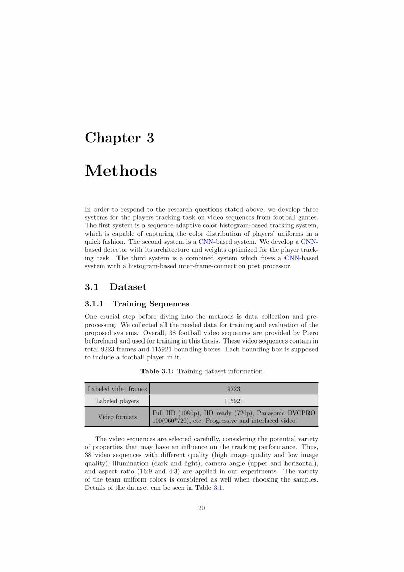
One crucial step before diving into the methods is data collection and pre-processing. We collected all the needed data for training and evaluation of theproposed systems. Overall, 38 football video sequences are provided by Pierobeforehand and used for training in this thesis. These video sequences contain intotal 9223 frames and 115921 bounding boxes. Each bounding box is supposedto include a football player in it.

Table 3.1: Training dataset information

Labeled video frames 9223

Labeled players 115921

Video formatsFull HD (1080p), HD ready (720p), Panasonic DVCPRO100(960*720), etc. Progressive and interlaced video.

The video sequences are selected carefully, considering the potential varietyof properties that may have an influence on the tracking performance. Thus,38 video sequences with different quality (high image quality and low imagequality), illumination (dark and light), camera angle (upper and horizontal),and aspect ratio (16:9 and 4:3) are applied in our experiments. The varietyof the team uniform colors is considered as well when choosing the samples.Details of the dataset can be seen in Table 3.1.

20

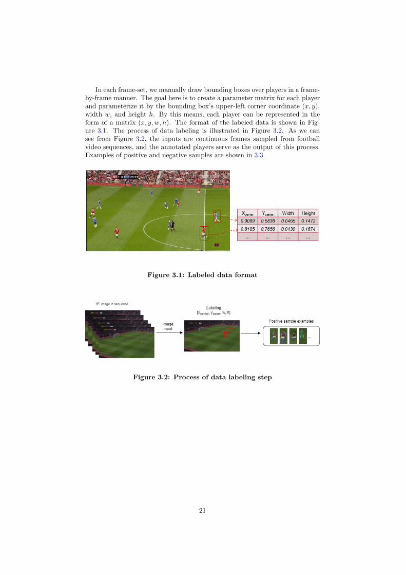
In each frame-set, we manually draw bounding boxes over players in a frame-by-frame manner. The goal here is to create a parameter matrix for each playerand parameterize it by the bounding box’s upper-left corner coordinate (x, y),width w, and height h. By this means, each player can be represented in theform of a matrix (x, y, w, h). The format of the labeled data is shown in Fig-ure 3.1. The process of data labeling is illustrated in Figure 3.2. As we cansee from Figure 3.2, the inputs are continuous frames sampled from footballvideo sequences, and the annotated players serve as the output of this process.Examples of positive and negative samples are shown in 3.3.

Figure 3.1: Labeled data format

Figure 3.2: Process of data labeling step

21

Figure 3.3: Examples of negative and positive samples

The details of the training dataset are shown in Table 3.2. Here, BBs Numberrefers to the number of bounding boxes. AvgW means the average width of allthe bounding boxes, and AvgH represents the average height of all the boundingboxes.

3.1.2 Testing Sequences

For the evaluation process, we prepare and use two different sequences in thisthesis, which vary in certain characteristics. Frame examples from these twosequences are shown here as in Figure 3.4 and 3.5. As is shown in Figure 3.4,the first testing sequence has a brighter background than the second one inFigure 3.5. The size of players in the first sequence is generally larger than thatin the second sequence. We can also notice that the first sequence has a muchbetter image resolution than the second one.

In this thesis, the proposed three systems are evaluated against benchmarks,such as YOLO and Faster R-CNN, on these two testing sequences. The obtainedresults should indicate how well the proposed systems generalize on differentfootball videos.

22

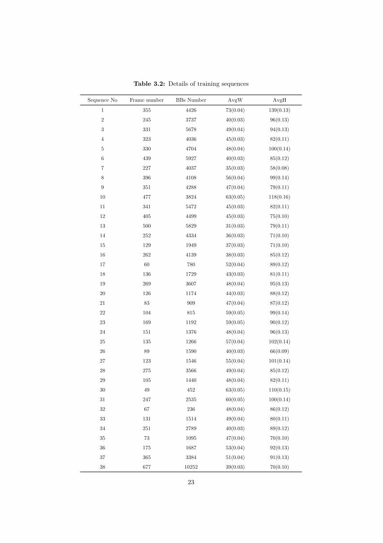
Table 3.2: Details of training sequences

Sequence No Frame number BBs Number AvgW AvgH

1 355 4426 73(0.04) 139(0.13)

2 245 3737 40(0.03) 96(0.13)

3 331 5678 49(0.04) 94(0.13)

4 323 4036 45(0.03) 82(0.11)

5 330 4704 48(0.04) 100(0.14)

6 439 5927 40(0.03) 85(0.12)

7 227 4037 35(0.03) 58(0.08)

8 396 4108 56(0.04) 99(0.14)

9 351 4288 47(0.04) 79(0.11)

10 477 3824 63(0.05) 118(0.16)

11 341 5472 45(0.03) 82(0.11)

12 405 4499 45(0.03) 75(0.10)

13 500 5829 31(0.03) 79(0.11)

14 252 4334 36(0.03) 71(0.10)

15 129 1949 37(0.03) 71(0.10)

16 262 4139 38(0.03) 85(0.12)

17 60 780 52(0.04) 89(0.12)

18 136 1729 43(0.03) 81(0.11)

19 269 3607 48(0.04) 95(0.13)

20 126 1174 44(0.03) 88(0.12)

21 83 909 47(0.04) 87(0.12)

22 104 815 59(0.05) 99(0.14)

23 169 1192 59(0.05) 90(0.12)

24 151 1376 48(0.04) 96(0.13)

25 135 1266 57(0.04) 102(0.14)

26 89 1590 40(0.03) 66(0.09)

27 123 1546 55(0.04) 101(0.14)

28 275 3566 49(0.04) 85(0.12)

29 105 1440 48(0.04) 82(0.11)

30 49 452 63(0.05) 110(0.15)

31 247 2535 60(0.05) 100(0.14)

32 67 236 48(0.04) 86(0.12)

33 131 1514 49(0.04) 80(0.11)

34 251 2789 40(0.03) 89(0.12)

35 73 1095 47(0.04) 70(0.10)

36 175 1687 53(0.04) 92(0.13)

37 365 3384 51(0.04) 91(0.13)

38 677 10252 39(0.03) 70(0.10)

23

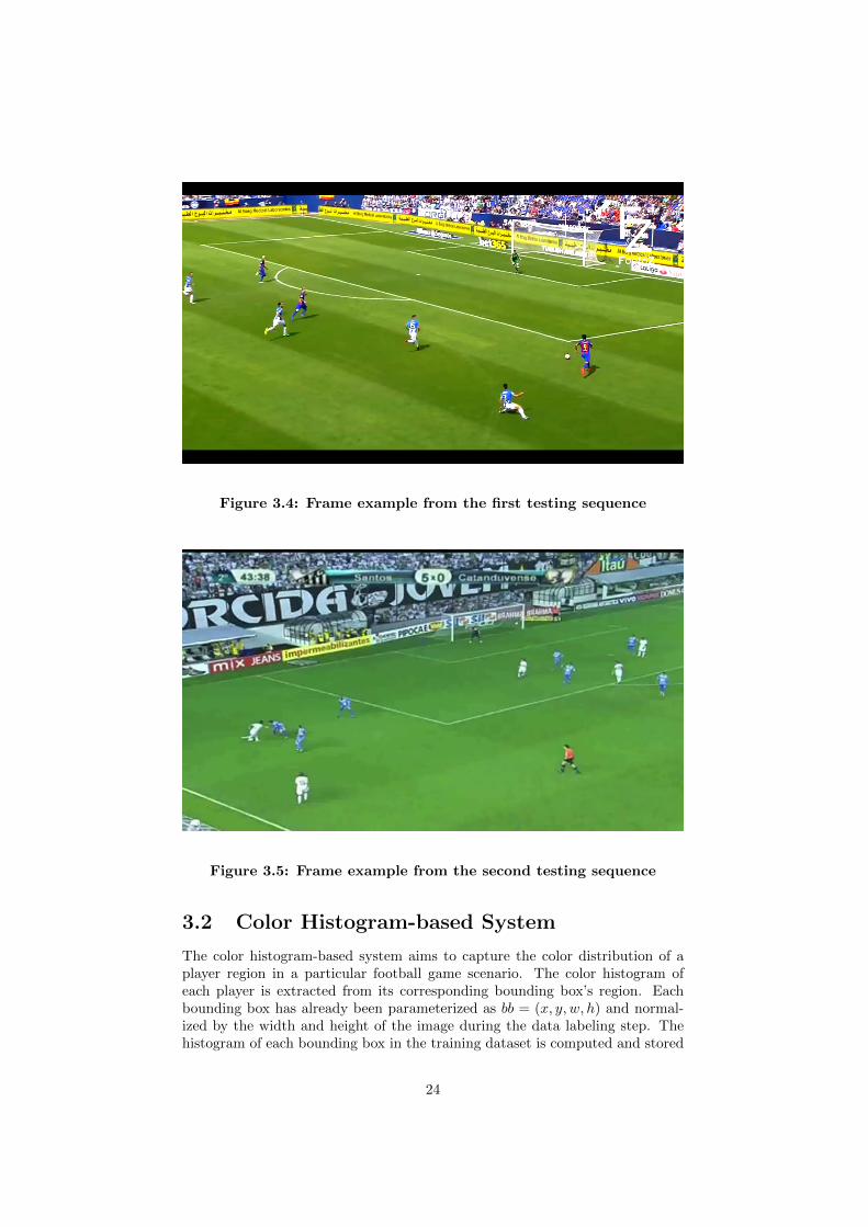
Figure 3.4: Frame example from the first testing sequence

Figure 3.5: Frame example from the second testing sequence

3.2 Color Histogram-based System

The color histogram-based system aims to capture the color distribution of aplayer region in a particular football game scenario. The color histogram ofeach player is extracted from its corresponding bounding box’s region. Eachbounding box has already been parameterized as bb = (x, y, w, h) and normal-ized by the width and height of the image during the data labeling step. Thehistogram of each bounding box in the training dataset is computed and stored

24

in a player histogram matrix HPL, which is involved in an improvement stepfor robust player tracking.

3.2.1 Color Histogram Distribution

To calculating the color histogram, we select the RGB feature of images to bethe detection feature. In order to decrease the computational complexity, effortsare made to reduce the dimension of the color histogram representation. Insteadof using a jointly distributed color space, we create a color model by mergingthe RGB histograms into a single vector and flattening it as h = [hR, hG, hB ].By this means, we divide each color channel into 16 bins and build the RGBhistogram into a one-dimensional flat vector, which contains in total 48 bins.

3.2.2 Evaluation of Similarity

The histogram-based system relies on the histogram similarity of detections be-tween consecutive frames to track players. Initially, the system is provided witha set of manually-drawn bounding boxes in the first frame. Then for the nextframe, each bounding box will shift around the previous position within a regionand calculate the histogram similarity between the newly-shifted bounding boxand the previously-stored one. The one with the highest similarity will be cho-sen as the new position of the bounding box. This process can then be iteratedand player tracking across frames can therefore be achieved.

There exist different methods to evaluate the histogram similarity betweenpredictions in the current frame and the target in the previous frame. In thissections, we mainly focus on two methods for this purpose, namely the histogramintersection and the square root of histogram difference.

Histogram Intersection

The paper [47] proposed a technique called Histogram Intersection. As stated inthis paper, the histogram has its own advantage in dealing with real-time index-ing problems with the sizeable pre-stored database. The histogram intersectionis considered robust since accurate separations of objects from the backgroundare not required by this method.

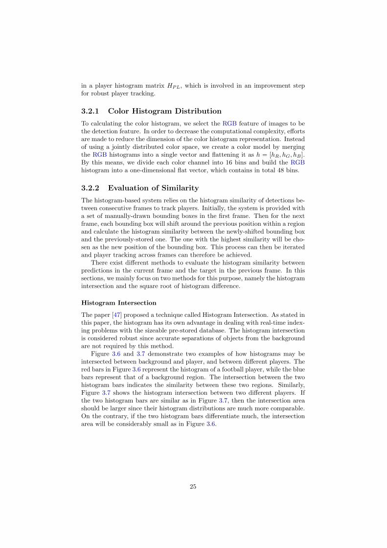
Figure 3.6 and 3.7 demonstrate two examples of how histograms may beintersected between background and player, and between different players. Thered bars in Figure 3.6 represent the histogram of a football player, while the bluebars represent that of a background region. The intersection between the twohistogram bars indicates the similarity between these two regions. Similarly,Figure 3.7 shows the histogram intersection between two different players. Ifthe two histogram bars are similar as in Figure 3.7, then the intersection areashould be larger since their histogram distributions are much more comparable.On the contrary, if the two histogram bars differentiate much, the intersectionarea will be considerably small as in Figure 3.6.

25

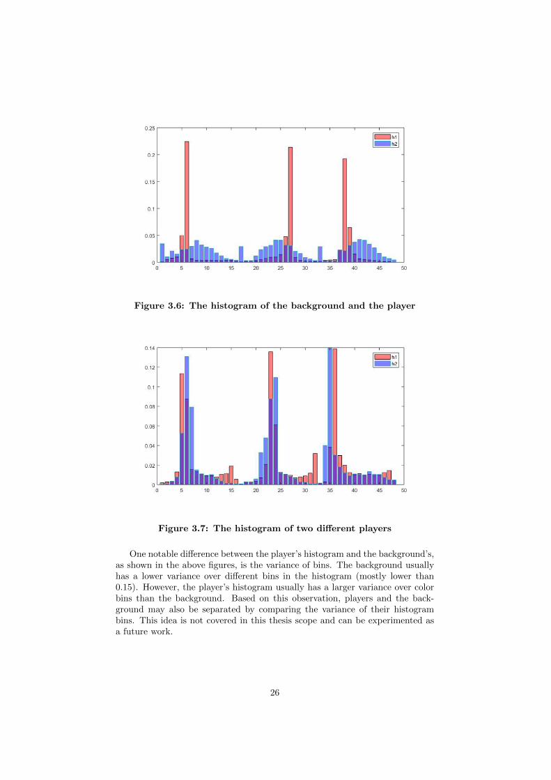
Figure 3.6: The histogram of the background and the player

Figure 3.7: The histogram of two different players

One notable difference between the player’s histogram and the background’s,as shown in the above figures, is the variance of bins. The background usuallyhas a lower variance over different bins in the histogram (mostly lower than0.15). However, the player’s histogram usually has a larger variance over colorbins than the background. Based on this observation, players and the back-ground may also be separated by comparing the variance of their histogrambins. This idea is not covered in this thesis scope and can be experimented asa future work.

26

Square Root of Histogram Difference

Another way to express the histogram similarity is to calculate the square root ofthe histogram difference, or in other words the distance between two histograms,as shown in equation 3.1. Hcurrentp, t represents the histogram of a derivedbounding box p in the current frame t, while Hpreviousq, t − 1 refers to thatof a bounding box q in the previous frame t− 1.

Dpreviousp, q, t =√

(Hcurrentp, t −Hpreviousq, t− 1)2 (3.1)

In order to improve the robustness of the histogram-based system, we alsocalculate the distanceDstored between the histogram of currently derived bound-ing boxes and that of the stored player annotations HPL from the training data,as shown in equation 3.2. A weight parameter α is applied here to take bothDprevious and Dstored into consideration when deciding the final detection. Asis shown in equation 3.3, the larger value the parameter α takes, the higherweight is assigned to the previous histogram distance than the stored histogramdistance.

Dstoredi, p, t =√

(Hcurrentp, t −HPLi)2 (3.2)

Dadjust = (1− α) ∗Dstored + α ∗Dprevious (3.3)

Here Dadjust is the adjusted distance. Dstored represents the least histogramdistance between the current bounding boxes and the stored ones, and Dprevious

means the least histogram distance between bounding boxes in the current frameand those in the last frame.

In this thesis, we choose the above histogram distance over histogram inter-section as our similarity evaluation metric due to the relative simplicity of itsexpression and the robustness.

3.3 CNN-based System

3.3.1 Network Architecture of CNN

Another proposed system in this thesis is the CNN-based system, in which aCNN architecture is designed and fine-tuned with the training video sequences.The network architecture of the CNN-based system is shown in Table 3.3.

As we can see from Table 3.3, the CNN network is designed to contain 8convolutional layers and 4 max-pooling layers for football player detection. Thedepth of the network is optimized to achieve a desired detection accuracy. Figure3.8 briefly illustrates the architecture of the CNN-based system.

27

Table 3.3: CNN-based system network architecture

# Layer Filters Size/Stride Input Output

0 conv 16 3 × 3 / 1 640 × 368 × 3 640 × 368 × 16

1 max 2 × 2 / 2 640 × 368 × 16 320 × 184 × 16

2 conv 32 3 × 3 / 1 320 × 184 × 16 320 × 184 × 32

3 max 2 × 2 / 2 320 × 184 × 32 160 × 92 × 32

4 conv 64 3 × 3 / 1 160 × 92 × 32 160 × 92 × 64

5 max 2 × 2 / 2 160 × 92 × 64 80 × 46 × 64

6 conv 128 3 × 3 / 1 80 × 46 × 64 80 × 46 × 128

7 max 2 × 2 / 2 80 × 46 × 128 40 × 23 × 128

8 conv 256 3 × 3 / 1 40 × 23 × 128 40 × 23 × 256

9 conv 512 3 × 3 / 1 40 × 23 × 256 40 × 23 × 512

10 conv 512 3 × 3 / 1 40 × 23 × 512 40 × 23 × 512

11 conv 5 1 × 1 / 1 40 × 23 × 512 40 × 23 × 5

Figure 3.8: Illustration of network architecture of CNN-based system.

28

3.3.2 Training

Transfer learning is used for training our CNN-based system. The first 8 lay-ers of our CNN-based system in Table 3.3 are directly initialized with weightparameters from the pre-trained Tiny-Yolo-V2 model. For the last four layers,weights are randomly initialized. During training, weight parameters from allthe layers are fine-tuned and adjusted based on our football training data.

The training of the CNN-based system is achieved using a Graphics Process-ing Unit (GPU). The memory requirement for the training is 4 Gigabytes.

3.4 Combined System

In order to use the CNN-based system while also taking advantage of play-ers’ visual appearance information, we combine the above two systems. Thiscombined system CNN-Inter Frame Connection is related to the algorithms pre-sented in [30] and [48], which combine a CNN-based detector with a tracklethandling post-processor [49]. To improve the readability, “combined system” or“CNN-IFC” is used to refer to this system in the rest of the presentation. Thissystem is proposed and developed as a potential way to boost the performance ofthe CNN-based system and the histogram-based system. The histogram-basedsequence-adaptive algorithm is updated and applied behind the CNN-based sys-tem as a post-processing module.

The two main parts in this combined system are the CNN detector and thehistogram-based post-processing module. The CNN detector simply shares thesame CNN architecture as in Figure 3.8, and it has been well covered in Section3.3. Therefore, this section is started with an introduction of the histogram-based post-processing module, and then follows a walk-through of the workflowof the combined system.

3.4.1 Histogram-based Post Processor

There are three major steps conducted by the histogram-based post processor,namely data association, adaptation of probability, and tracklet ID handling.Note that these steps are performed right after the CNN detector outputs initialregion proposals of players. The common practice used in CNN that proposalsare filtered with a confidence threshold is delayed to the third step.

In order to associate detections in the previous frame Φn−1 with the propos-als in the current frame, the data association step is applied to calculate a scorematrix D between detection pairs. It measures the distance between a detectedbounding box in frame n−1 and that in frame n. The distance here is defined asDij = 0.25 ‖Xi −Xj‖+ 0.50 ‖Hi −Hj‖+ 0.25 |Pi − Pj |. X = [x, y, w, h] is theparameterized vector of a bounding box, and H represents the color histogramof a bounding box. P indicates the inferred probability that a bounding boxcontains a player. A higher weight is specifically assigned to the color histogramterm to reflect the fact that color information plays a crucial role in player track-ing in football videos. The pseudo code of the data association step is attachedas below. Ψn represents the proposals in the current frame.

29

Algorithm 1: Data Association

Data: Φn−1, Ψn

Result: Accepted mappings set Ω1 begin

// Initialization

2 Initialize connected pairs set Υ and accepted mappings set Ω;

3 for i ∈ Φn−1 do4 for j ∈ Ψn do

5 Calculate the matching score Dij and store it in a scorematrix D.

6 end

7 end

8 while Φn−1 6= ∅ and Ψn 6= ∅ do

9 Find the pair (imin, jmin) with the minimum score in D.

10 Append the selected pair into Υ as Υ = Υ ∪(imin, jmin

).

11 Remove imin and jmin from Φn−1 and Ψn respectively.

12 end

13 for(i, j)∈ Υ do

14 if(|xi − xj |+ |yi − yj |

)≤ 1

2

(ωi+ωj

2 +hi+hj

2

)then

15 Append pair (i, j) into the final accepted mappings set Ω.16 end

17 end

18 end

The adaptation of probability aims to compensate the probability P when anunexpected probability drop takes place. As is demonstrated in the pseudo codebelow, a threshold Θmin is determined based on the color histogram distancebetween detected bounding boxes in two consecutive frames. If ‖Hi −Hj‖ issmaller than 0.1, it means the color histogram distributions of these boundingboxes are considered similar with a high confidence. We should then set Θmin

aggressively to 0.2 so that the probability adaptation can be triggered easily. If‖Hi −Hj‖ is larger than 0.1, we should set Θmin conservatively to 0.4 to raisethe bar for probability adaptation in such case. After Θmin is determined, Pn

j

is updated based on the equation Pnj = (1 − α) Pn

j + α Pn−1i . α is selected

as 0.98 in our implementation. This step is designed to mitigate unexpectedprobability drops for region proposals in the current frame, and it is expectedto improve the system performance in terms of a better recall rate.

30

Algorithm 2: Probability Adaptation

Data: Accepted mappings set Ω, Φn−1, Ψn

Result: Mappings set with adjusted probabilities1 begin

// Probability Adaptation

2 for(i, j)∈ Ωn,n−1 do

3 Determine Θmin based on the histogram distance ‖Hi −Hj‖.

4 if(Pn−1i > Pn

j

)and

(Pnj > Θmin

)then

5 Update Pnj : Pn

j = (1− α) Pnj + α Pn−1

i .

6 end

7 end

8 end

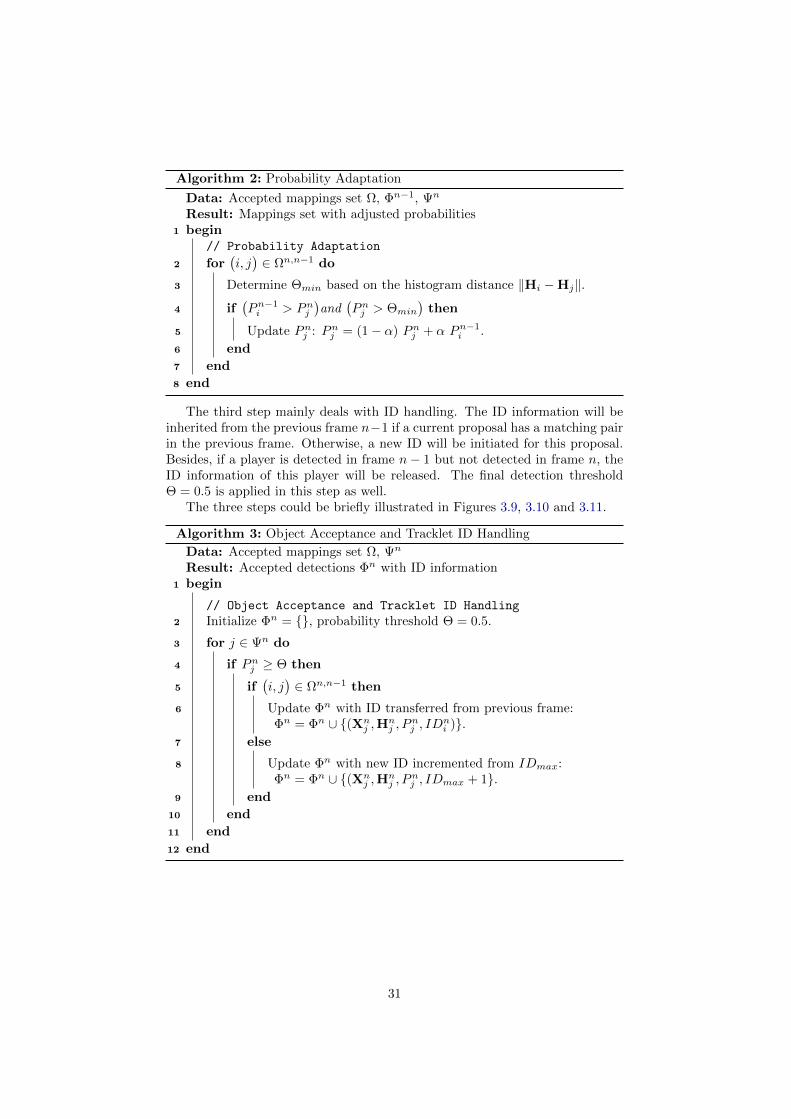
The third step mainly deals with ID handling. The ID information will beinherited from the previous frame n−1 if a current proposal has a matching pairin the previous frame. Otherwise, a new ID will be initiated for this proposal.Besides, if a player is detected in frame n− 1 but not detected in frame n, theID information of this player will be released. The final detection thresholdΘ = 0.5 is applied in this step as well.

The three steps could be briefly illustrated in Figures 3.9, 3.10 and 3.11.

Algorithm 3: Object Acceptance and Tracklet ID Handling

Data: Accepted mappings set Ω, Ψn

Result: Accepted detections Φn with ID information1 begin

// Object Acceptance and Tracklet ID Handling

2 Initialize Φn = , probability threshold Θ = 0.5.

3 for j ∈ Ψn do

4 if Pnj ≥ Θ then

5 if(i, j)∈ Ωn,n−1 then

6 Update Φn with ID transferred from previous frame:Φn = Φn ∪ (Xn

j ,Hnj , P

nj , ID

ni ).

7 else

8 Update Φn with new ID incremented from IDmax:Φn = Φn ∪ (Xn

j ,Hnj , P

nj , IDmax + 1.

9 end

10 end

11 end

12 end

31

Figure 3.9: Data Association Step: In order to associate the detec-tions from the previous frames to the proposals in the current frame.

Figure 3.10: Probability Adaptation Step: In the figure, one of thedetection probability of the region proposal in frame n is increased.For a better understanding, we use the thickness of the boundingboxes to represent the probability.

Figure 3.11: Tracklet Handling Step: Final thresholding will be ap-plied in this step. This step is dealing with the transfer for the trackID.

3.4.2 Workflow

The workflow of the combined system can be summarized from a black-boxmodel perspective. Consecutive frames with resolution 640 × 368 in RGB arefed into the combined system as inputs, in which the CNN model generatesaccordingly 40× 23 region proposals. These proposals would be further filteredby a non-maximum suppression [50] algorithm. JNMS is used here to denotethe number of region proposals after the non-maximum suppression algorithm.

32

After getting the initial proposals from the CNN, the combined system willgo through the three steps as mentioned above and generate final detections.The obtained detections in the current frame will be determined not only basedon the available region proposals Ψn in the current frame but also the relevantdetections Φn−1 from the previous frame. The whole process is illustrated inFigure 3.12.

Figure 3.12: The workflow of the combined system

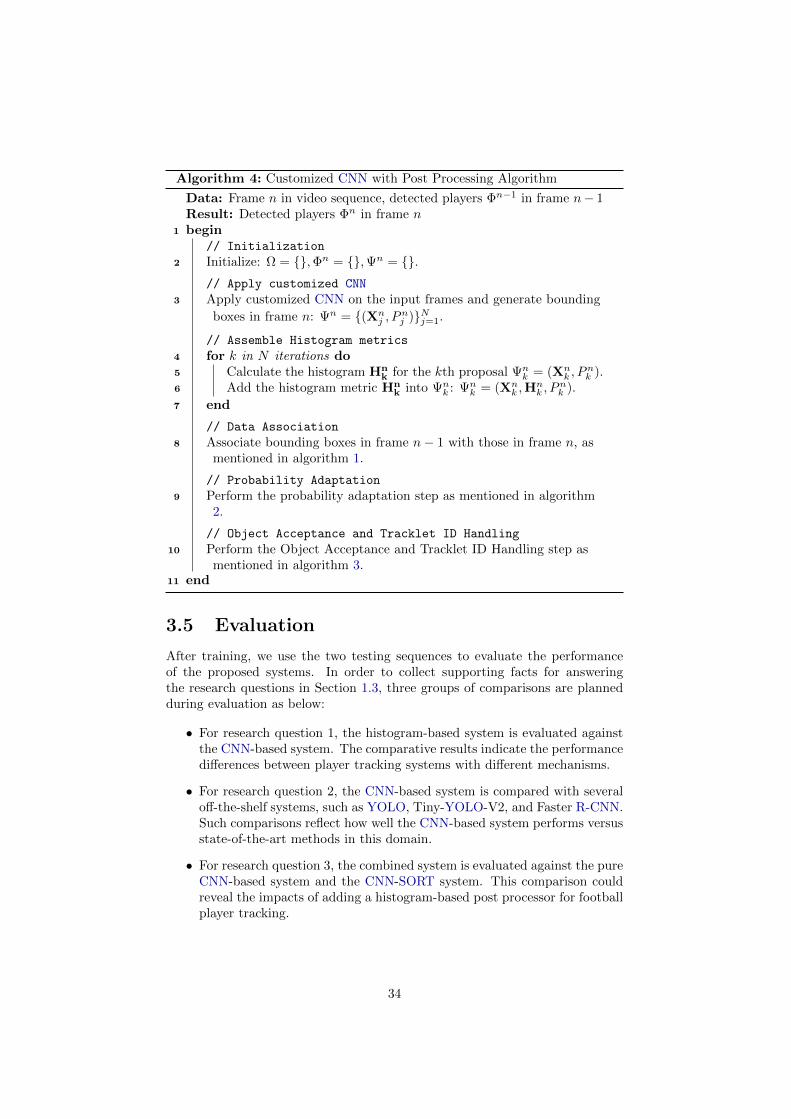
The process can also be briefly outlined in the pseudo code below as inAlgorithm 4. The combined system takes frame sequences sampled from thefootball video clips as inputs and returns a set of detected proposals in eachframe as outputs. The input data is firstly processed by a fine-tuned CNNmodel, and then it will be processed by the histogram-based post-processor.

33

Algorithm 4: Customized CNN with Post Processing Algorithm

Data: Frame n in video sequence, detected players Φn−1 in frame n− 1Result: Detected players Φn in frame n

1 begin// Initialization

2 Initialize: Ω = ,Φn = ,Ψn = .// Apply customized CNN

3 Apply customized CNN on the input frames and generate bounding

boxes in frame n: Ψn = (Xnj , P

nj )Nj=1.

// Assemble Histogram metrics

4 for k in N iterations do5 Calculate the histogram Hn

k for the kth proposal Ψnk = (Xn

k , Pnk ).

6 Add the histogram metric Hnk into Ψn

k : Ψnk = (Xn

k ,Hnk , P

nk ).

7 end

// Data Association

8 Associate bounding boxes in frame n− 1 with those in frame n, asmentioned in algorithm 1.

// Probability Adaptation

9 Perform the probability adaptation step as mentioned in algorithm2.

// Object Acceptance and Tracklet ID Handling

10 Perform the Object Acceptance and Tracklet ID Handling step asmentioned in algorithm 3.

11 end

3.5 Evaluation

After training, we use the two testing sequences to evaluate the performanceof the proposed systems. In order to collect supporting facts for answeringthe research questions in Section 1.3, three groups of comparisons are plannedduring evaluation as below:

• For research question 1, the histogram-based system is evaluated againstthe CNN-based system. The comparative results indicate the performancedifferences between player tracking systems with different mechanisms.

• For research question 2, the CNN-based system is compared with severaloff-the-shelf systems, such as YOLO, Tiny-YOLO-V2, and Faster R-CNN.Such comparisons reflect how well the CNN-based system performs versusstate-of-the-art methods in this domain.

• For research question 3, the combined system is evaluated against the pureCNN-based system and the CNN-SORT system. This comparison couldreveal the impacts of adding a histogram-based post processor for footballplayer tracking.

34

3.5.1 Evaluation Metrics

In order to assess the performances of the proposed systems in a quantitativeway, the following evaluation metrics are measured during experiments:

Precision evaluates the fraction of the true positive detected bounding boxesamongst the retrieved predictions, or in other words the ratio of the detectedpositive players to all the detected players. It is calculated as equation 3.4.

Precision =True positive predictions

All predictions(3.4)

Another important metric in this thesis is referred to as recall, which repre-sents the ratio of the positive detections to all the ground truth detections. Itindicates how much proportion of the ground truths can be detected as positive.The calculation of recall is shown in equation 3.5.

Recall =True positive predictions

Ground truths(3.5)

In this thesis, the correctness of detection is defined by the area of intersec-tion between a prediction and a ground truth. The parameter IOU is used torepresent this metric, which can be calculated as equation 3.6:

IOU =area(Bp ∩Bt)

area(Bp ∪Bt)(3.6)

Here Bp denotes the predicted bounding box and Bt denotes the groundtruth. In the histogram-based system, only those detected bounding boxes thathave a larger IOU value than 0.6 are regarded as positive detections. One groundtruth can then only be assigned to one detected box according to the maximumIOU. If more than one predictions are assigned to the same ground truth, onlyone of the bounding boxes is taken as a valid detection. Other detected boxesare manually reset to have zero IOU and will not be considered when calculatingthe average IOU of all the detections. On the other hand, one ground truth canalso be only assigned to one detected box according to the maximum IOU. Thesystem will be penalized in the same manner if the rule above is conflicted.

F1 score is selected when comparing the combined system with benchmarks.The metric F1 is calculated based on Equation 3.7. It conveys the harmonicmean of precision and recall.

F1 = 2× Recall× Precision

Recall + Precision(3.7)

Another evaluation metric is Identity Tracking Performance (ITP) [51]. Itcalculates the ratio of the number of correct ID to the number of ground truths[51] as shown in equation 3.8.

ITP =#Correct ID

#Ground truth(3.8)

35

Chapter 4

Experiment Results

4.1 Histogram-based System

4.1.1 Positive Detections

Positive detection results of the histogram-based system are shown in Figure4.1. The two pictures on the first row are from the high-quality video sequence,while the second row comes from the low-quality one. Results on the high-quality testing sequence have shown that the system is capable of detectinga player or part of a player on the edge of a video frame. It demonstratesa decent tracking performance, especially when players have contrasting colordistributions compared to the background. On the other hand, the system hasproven to be well tolerant of poor image quality and dark background based onthe results on the low-quality testing sequence.

Figure 4.1: Positive detections made by the histogram-based system.

36

4.1.2 Negative Detections

In spite of the positive examples above, there also exist some negative detections,as shown in Figure 4.2. At least one negative detection can be observed in eachof the four subfigures. In these negative examples, the system fails to overlayplayers with bounding boxes correctly. Instead, the background is misidentifiedas a player. In the top two pictures, negative detections appear when two playersstay a fairly close distance to each other. With the players moving continuously,one of the bounding boxes covers the two players, and the other one moves awayfrom the player’s region. Since negative detections usually happen when playersare moving fast, we could associate the failure of player tracking with the motionblur in football videos. The reason may be that the color histogram of a motionblur region approaches that of a background region better than a player region.Therefore, such false-positive detections are naturally more likely to happen inthis case.

Figure 4.2: Negative detections made by the histogram-based system.

4.2 CNN-based System

We evaluate the CNN-based system by injecting the testing sequences into thefine-tuned system. After thresholding the initial region proposals, we can get theselected proposal vectors, each of which contains the information of its position,size and the matching probabilities for a particular class. The precision-recallcurves can be obtained based on these filtered proposal vectors and the groundtruth at different thresholds, as in Figure 4.3 to 4.5. A trade-off relationship be-tween the precision and recall rate can be clearly observed from the curves. Thethreshold in each figure demonstrates above which confidence level a proposalis regarded as a ground truth. Only those proposals with higher probabilitiesthan the threshold will be selected as final predictions. When the threshold is

37

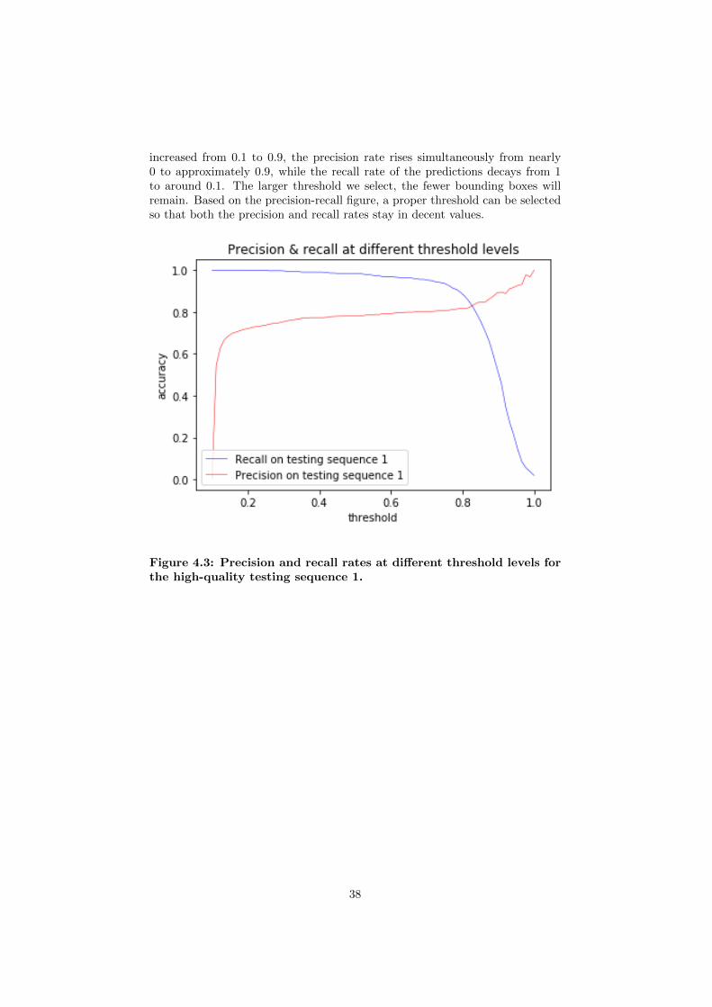
increased from 0.1 to 0.9, the precision rate rises simultaneously from nearly0 to approximately 0.9, while the recall rate of the predictions decays from 1to around 0.1. The larger threshold we select, the fewer bounding boxes willremain. Based on the precision-recall figure, a proper threshold can be selectedso that both the precision and recall rates stay in decent values.

Figure 4.3: Precision and recall rates at different threshold levels forthe high-quality testing sequence 1.

38

Figure 4.4: Precision and recall rates at different threshold levels forthe low-quality testing sequence 2.

4.2.1 Comparison between CNN-based System and Histogram-based System

For the proposed CNN-based system and histogram-based system, experimentsare conducted to compare their performances in terms of average IOU andprecision rate. Based on the same training and testing sequences, measures ofthese metrics in the two systems are listed in the below tables.

Table 4.1: Average Intersection over Union achieved by CNN-based systemand histogram-based system on two testing sequences.

Average IOU Testing sequence 1 Testing sequence 2

CNN-based system 0.87 0.85

Histogram-based system 0.76 0.73

As is shown in Table 4.1, the CNN-based system clearly outperforms thehistogram-based system with a higher average IOU for both testing sequences.

39

Figure 4.5: Precision-recall curves of histogram-based system andCNN-based systems on two different testing sequences.

As a complement of the above measures, the precision-recall curves of the twosystems are demonstrated in Figure 4.5 as well. Since there is no thresholding inthe histogram-based system, only one precision-recall sample is plotted for eachtesting sequence on the figure. Also, the CNN-based system outperforms thehistogram-based system in terms of both precision and recall rate, regardless ofwhat threshold is selected. As illustrated in Figure 4.5, a superior precision rateis achieved by the CNN-based system on both testing sequences, which provesthat the CNN-based system delivers a more accurate detecting performance.The detections provided by the CNN-based system should contain more truepositive region proposals than the histogram-based system.

4.2.2 Comparison between CNN-based System and Off-the-shelf Systems

The performance of CNN-based system is also compared with that of threedifferent off-the-shelf systems, namely Faster R-CNN, YOLO, and Tiny-YOLO-V2. Same testing sequences are fed into the off-the-shelf systems and our CNN-based system to generate final player detections and measures of the evaluationmetrics. Figure 4.6, 4.7, and 4.8 demonstrate respectively the detection resultsfrom Faster YOLO, Tiny-YOLO-V2, and Faster R-CNN alongside that fromthe proposed CNN-based system.

As is shown in Figure 4.6, our CNN-based system manages to recognizemore players than the YOLO system does. Only two players are detected inthis frame by YOLO in the left subfigure, while all the players are recognized

40

correctly by our CNN-based system in the right subfigure.

Figure 4.6: Detection results through YOLO system with pre-trainedmodel and our in-house CNN-based sports analytic system.

As for Tiny-YOLO-V2, it makes plenty of false positive predictions in Fig-ure 4.7. For examples, some audiences and background regions are incorrectlydetected as players. Besides, detection of the referee and certain players aremissing in the left subfigure.

Figure 4.7: Detection results through Tiny-YOLO-V2 system withpre-trained model and our in-house CNN sports analytic system.

41

Figure 4.8: Detection results through Faster R-CNN system withpre-trained model and our in-house CNN sports analytic system.

Faster R-CNN usually employs 9 anchor boxes, with 3 different sizes and 3width-height ratios, to generate region proposals. It is proved to normally showa superior performance than YOLO when detecting smaller objects. As is shownin Figure 4.8, the Faster R-CNN detector fails in recognizing all the players, butit generates no false positive detections. The CNN-based system manages torecognize more players than the Faster R-CNN detector since players usuallymake unique human postures during a football game compared to pedestrians.Training a system solely with regular human data resources is not adequate forthe detection of players in the football analytics field.

Evaluation of Detection Performance in terms of mAP

Measures of the evaluation metric mAP are collected here to benchmark thedetection performance of the CNN-based system against Faster R-CNN withVGG16 on 2 testing sequences of different image resolutions. YOLO and Tiny-YOLO-V2 are not compared since they have shown to deliver significantly worseperformances than the Faster R-CNN system as mentioned above.

Table 4.2: Evaluation of detection performance in terms of mAP.

System Testing sequence 1 Testing sequence 2

Faster R-CNN 0.60 0.19

CNN-based system 0.86 0.85

As table 4.2 indicates, Faster R-CNN falls short in the mAP measures inboth testing sequences since it is not fine-tuned for the football players detectionscenario, even though Faster R-CNN advances in the object detection domain.The result clearly demonstrates a superior detection performance of the CNN-based system over one of the best benchmarks. As the results reveal, the largestperformance difference happens at the low resolution sequence. The reason forsuch a significant performance delta is that the Faster R-CNN is typically trainedon common datasets which contain very limited blurs. As testing sequences 2 is alow image resolution sequence with a large amount of blurs, it is poorly handled

42

by the Faster R-CNN system but well managed by the fine-tuned CNN-basedsystem.

4.3 Combined System

4.3.1 Evaluation of Tracking Performance

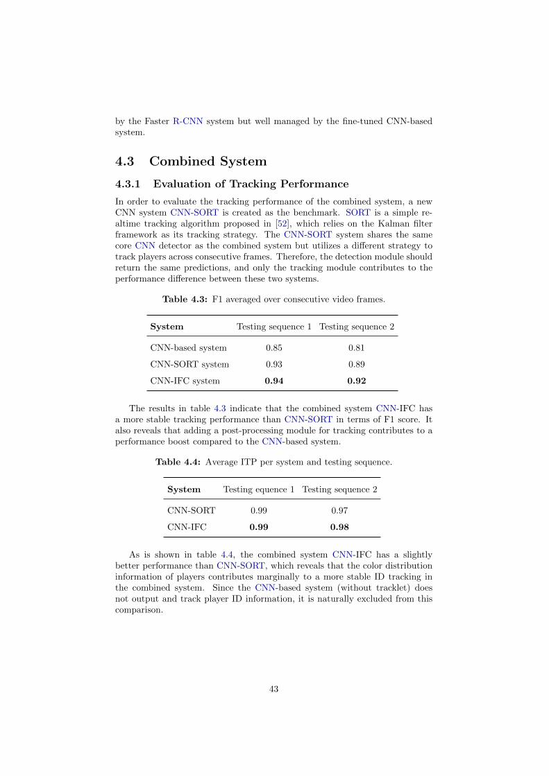
In order to evaluate the tracking performance of the combined system, a newCNN system CNN-SORT is created as the benchmark. SORT is a simple re-altime tracking algorithm proposed in [52], which relies on the Kalman filterframework as its tracking strategy. The CNN-SORT system shares the samecore CNN detector as the combined system but utilizes a different strategy totrack players across consecutive frames. Therefore, the detection module shouldreturn the same predictions, and only the tracking module contributes to theperformance difference between these two systems.

Table 4.3: F1 averaged over consecutive video frames.

System Testing sequence 1 Testing sequence 2

CNN-based system 0.85 0.81

CNN-SORT system 0.93 0.89

CNN-IFC system 0.94 0.92

The results in table 4.3 indicate that the combined system CNN-IFC hasa more stable tracking performance than CNN-SORT in terms of F1 score. Italso reveals that adding a post-processing module for tracking contributes to aperformance boost compared to the CNN-based system.

Table 4.4: Average ITP per system and testing sequence.

System Testing equence 1 Testing sequence 2

CNN-SORT 0.99 0.97

CNN-IFC 0.99 0.98

As is shown in table 4.4, the combined system CNN-IFC has a slightlybetter performance than CNN-SORT, which reveals that the color distributioninformation of players contributes marginally to a more stable ID tracking inthe combined system. Since the CNN-based system (without tracklet) doesnot output and track player ID information, it is naturally excluded from thiscomparison.

43

Chapter 5

Discussion and Conclusions

5.1 Limitations

The acquired results during experiments are limited to some extent and maymuch vary depending on the experiment settings. In this section, potentiallimitations and impact factors are discussed as follows.

5.1.1 Dataset

As the major input of model training, the dataset may impact the performanceof the proposed systems. Important aspects of the dataset, such as quantity,quality, and variety, are briefly covered in this sub-section.

First of all, the quantity of the training data plays an essential role in in-fluencing the systems’ performances. Training a network model with a limitedamount of data may result in model overfitting and degraded generalization.In our experiments, we manually labeled 115921 players in 9223 selected videoframes. It remains unknown whether such amount of data samples are substan-tial for network training in this case.

Besides, the quality of the prepared training data should be taken into con-sideration since carelessly-prepared frame images may end up “fooling” thetrained networks. For instance, when labeling players with strong motion blurs,we may accidentally draw bounding boxes with a poor accuracy. Therefore, er-rors can be expected between our data annotations and the “real-world” groundtruths, causing a potential decline in the quality of the training data.

The variety of the training data is another vital factor of neural networktraining. The data samples used in this thesis are collected from real-timevideos of football games. These videos are carefully selected to guarantee acomprehensive coverage of diverse game scenarios, such as different image res-olutions, player sizes, and light conditions. However, there still exists varioussituations that are not covered due to the limitation of our data source, andthe generalization of the proposed systems may thus be impacted negatively.For example, weather conditions are not thoroughly considered in this thesis.When football games collide with extreme weather events (e.g. rain or snow),the proposed systems may not work as expected since they have insubstantialknowledge about such unseen scenarios.

44

5.1.2 YOLO

In both the CNN-based system and the combined system, YOLO is applied asa pre-trained model and fine-tuned with the selected football video sequences.Consequently, the performance of these systems may be affected by the settingsof the YOLO model.

First of all, the number of grid cells configured in the YOLO model mayimpact the detection performance. When YOLO is used for detection tasks, aninput image is typically divided into S × S grid cells. Each grid cell is assumedto contain only one object. This assumption may lose its validity when multipleobjects or players in our case stay fairly close to each other. Some overlappedplayers may not be easily detected with a scarce number of configured gridcells. On the other hand, if an input image is densely distributed with gridcells, a single player may be segmented by multiple grid cells and thus overlaidwith numerous bounding boxes. Such practice increases computational cost fortraining and may solely bring limited gain in detection accuracy. YOLO may failin learning to separate closely-located players if such cases occur infrequently inthe training dataset. The granularity of grid cells in our case is experimentallyfound based on how crowed the players are distributed in the ground truth data.The performance may be impacted if the choice of the granularity is driven byother means.

Another aspect of YOLO that may impact the performance is the networkarchitecture. In this thesis, we trim a Tiny-YOLO-V2 model to preserve its first8 layers and fuse them with additional 4 convolutional layers in our CNN-basesystem and the combined system. The architecture is determined and optimizedbased on the current provided dataset and may need further refinements tocope with various data inputs in the future. For example, if image samples ofrainy or snowy football games are included in the dataset, the current networkarchitecture may need a scale-up to handle such new scenarios. Then keepingup to the first 10 or 12 layers of the Tiny-YOLO-V2 model could be a feasiblesolution in this case.

5.1.3 Histogram-based System

The proposed histogram-based system in this thesis does not rely on neuralnetworks and requires no network training. It is easily deployed but may notguarantee a matching quality of the tracking-by-detection results.

There are generally three major factors that may impact its performance.First of all, the initialization of the bounding boxes at the first frame is a crucialfactor since it determines the reference color histogram of the targeted players.Drawing a bounding box on top of a player with an inappropriate size or positionmay pollute the reference histogram with irrelevant color information and causea drop of detection accuracy.

Besides, each bounding box is moved around its current position within aregion to derive proposals of the targeted player in the next frame. The regionsize is correlated with the sampling rate of frames. If two consecutive framesare sampled between a short interval from an video clip, then the position of aplayer should not differ much between two frames. A small region in this caseshould be adequate to capture the transition. On the contrary, a relative largeregion is required to cope with a low sampling rate since players may move far

45

away in the current frame from their previous positions. A lousy setting of theregion size may result in an unexpected performance degradation.

Lastly, the performance of histogram-based system is negatively affected bymotion blurs. When motion blurs happen, the region proposals may have a sim-ilar color histogram distribution as the background. Then using the histogramsimilarity as the sole criterion would make the histogram-based system sufferfrom this disturbance.

5.2 Conclusions

In this thesis, we first propose a sequence-adaptive histogram-based system anda customized CNN-based system to tackle the challenging problem of multi-players tracking in football video sequences. The sequence-adaptive histogram-based system associates player detections at the past frame with region pro-posals at the current frame. Based on the assumption that players move withlinear velocity between short time intervals, the computational complexity of thehistogram-based system is considerably reduced. The customized CNN-basedsystem is fine-tuned from Tiny-YOLO-V2 with the architecture and weightsoptimized for the football player tracking-by-detection task. In addition, thisthesis provides a recipe for the customization of a tracking-by-detection sys-tem. We combine the above two systems by concatenating a sequence-adaptivehistogram-based post-processor to the CNN-based system. The combined sys-tem is expected to leverage the advantages of the CNN-based system whilemaking full use of players’ visual appearance characteristics.

Based on the experiment results and related analysis, we can conclude thisthesis by answering the research questions in Section 1.3:

• For question 1, both the histogram-based system and CNN-based systemmanage to track football players across consecutive video frames. Exper-iment results indicate that the CNN-based system generally outperformsthe histogram-based system in terms of a higher mean IOU, precision andrecall rate on the testing sequences.

• For question 2, experiments are conducted to benchmark the performanceof the CNN-based system against off-the-shelf systems, such as Faster-R-CNN. Results reveal that our CNN-based system delivers a superiorperformance than its benchmarks in terms of a higher mAP on the testingsequences. Fine-tuning the CNN-based system specifically with footballvideo sequences prepares it with the knowledge about the characteristicsof football players and motion blurs. This practice contributes to such aperformance boost for players tracking-by-detection in football videos.

• For question 3, we evaluate the performance of the combined systemagainst the pure CNN-based system and the CNN-SORT system. Resultsdemonstrate that the combined system performs better than its bench-marks. Based on the result, it can be concluded that adding a histogram-based post-processor to the CNN-based system could significantly improveits tracking performance. Also, this fused pattern opens up the possibilityto adjust the detection probability based on the dominant characteristicsof a detection task.

46

5.2.1 Future Work

For the combined system, we can try other post-processor adaptive detectorsbased on the jersey color of each team in order to differentiate teams in thefuture. It is considered much tricky to accomplish this task if we use a pureCNN-based system. Also, now we only train our CNN-based system on footballgames. In the future, we can adapt it to other types of sports, such as basketballor baseball games. As mentioned in the limitation section, in the future we canalso consider including scenarios of extreme weather when selecting trainingdata.

47

Bibliography

[1] S. S. Intille and A. F. Bobick, “Closed-world tracking,” in Computer Vision,1995. Proceedings., Fifth International Conference on. IEEE, 1995, pp.672–678.

[2] A. Bewley, Z. Ge, L. Ott, F. Ramos, and B. Upcroft, “Simple online andrealtime tracking,” in Image Processing (ICIP), 2016 IEEE InternationalConference on. IEEE, 2016, pp. 3464–3468.

[3] J. P. Omer Tene, “Privacy in the age of big data: A time for big decisions,”vol. 64, 01 2012.

[4] R. Wiles, J. Prosser, A. Bagnoli, A. Clark, K. Davies, S. Holland, andE. Renold, “Visual ethics: Ethical issues in visual research,” 2008.

[5] P. team, “Piero at red bee media,” https://www.redbeemedia.com/.

[6] P. Viola and M. Jones, “Robust real-time object detection,” in Interna-tional Journal of Computer Vision, 2001.

[7] W. Luo, J. Xing, A. Milan, X. Zhang, W. Liu, X. Zhao, and T.-K. Kim,“Multiple Object Tracking: A Literature Review,” ArXiv e-prints, Sep.2014.

[8] P. Nillius, J. Sullivan, and S. Carlsson, “Multi-target tracking-linking iden-tities using bayesian network inference,” in null. IEEE, 2006, pp. 2187–2194.

[9] M. D. Breitenstein, F. Reichlin, B. Leibe, E. Koller-Meier, and L. V. Gool,“Robust tracking-by-detection using a detector confidence particle filter,”in Proc.IEEE 12th International Conference on Computer Vision (ICCV),2009, pp. 142–14.

[10] W.-L. Lu, J.-A. Ting, K. P. Murphy, and J. J. Little, “Identifying playersin broadcast sports videos using conditional random fields,” in Proc. IEEEConference on Computer Vision and Pattern Recognition, 2011, pp. 3249–3256.

[11] J. Fan, W. Xu, Y. Wu, and Y. Gong, “Human tracking using convolutionalneural networks,” IEEE Transactions on Neural Networks, vol. 21, pp. 1610– 1623, 2010.

48

[12] Y. Li, A. Dore, and J. Orwell, “Online multiperson tracking by detectionfrom single uncalibrated camera,” in Proc.IEEE Transactions on PatternAnalysis and Machine Intelligence, vol. 33, 2011, pp. 1820–1833.

[13] R. E. Kalman, “A new approach to linear filtering and prediction prob-lems,” 1960.

[14] P. D. Moral, “Nonlinear filtering: Interacting particle resolution,” ComptesRendus de l’Academie des Sciences-Serie I-Mathematique, vol. 325, no. 6,pp. 653–658, 1997.

[15] J. Pers and S. Kovacic, “Computer vision system for tracking players insports games,” Image and Signal Processing and Analysis, 2000.

[16] K. Okuma, A. Taleghani, N. De Freitas, J. J. Little, and D. G. Lowe, “Aboosted particle filter: Multitarget detection and tracking,” in Europeanconference on computer vision. Springer, 2004, pp. 28–39.

[17] W. Campbell, D. Sturim, D. Reynolds, and A. Solomonoff, “AFL playerdetection and tracking,” in Proc. Digital Image Computing, 2016.

[18] O. Utsumi, K. Miura, and I. Ide, “An object detection method for describ-ing soccer games from video,” in Proc. IEEE ICME, 2002, pp. 45–48.

[19] G. R. Bradski, “Computer vision face tracking for use in a perceptualuser interface,” in Proc. IEEE Workshop Applications of Computer Vision,1998, pp. 214–219.

[20] S. K. Bidhendi and R. Safabakhsh, “Effective tracking of the players andball in indoor soccer games in the presence of occlusion,” in Proc. IEEE,Computer Conference, 2009, pp. 524–529.

[21] S. Gerke, K. Muller, and R. Schafer, “Soccer jersey number recognition us-ing convolutional neural networks,” in Proc IEEE International Conferenceon Computer Vision Workshop (ICCVW), 2016, p. 734– 741.

[22] E. Monier, P. Wilhelm, and U. Ruckert, “Template matching based trackingof players in indoor team sports,” Distributed Smart Cameras, 2009.

[23] Y. Ohno, J. Miura, and Y. Shirai, “Tracking players and a ball in soccergames,” in Proc. Int. Conf. Multisensor Fusion and Integration for Intelli-gent Sys, 1999.

[24] Y. Ming, C. Guodong, and Q. Lichao, “Player detection algorithm basedon gaussian mixture models background modeling,” in Proc.Second Inter-national Conference on Intelligent Networks and Intelligent Systems, 2009.

[25] P. Viola and M. Jones, “Rapid object detection using a boosted cascadeof simple features,” in Computer Vision and Pattern Recognition, 2001.CVPR 2001. Proceedings of the 2001 IEEE Computer Society Conferenceon, vol. 1. IEEE, 2001, pp. I–I.

[26] P. F. Felzenszwalb, R. B. Girshick, D. McAllester, and D. Ramanan,“Object detection with discriminatively trained part-based models,” IEEEtransactions on pattern analysis and machine intelligence, vol. 32, no. 9,pp. 1627–1645, 2010.

49

[27] Y. Seo, S. Choi, H. Kim, and K.-S. Hong, “Where are the ball and players?soccer game analysis with color-based tracking and image mosaick,” inInternational Conference on Image Analysis and Processing. Springer,1997, pp. 196–203.

[28] W.-L. Lu, J.-A. Ting, J. J. Little, and K. P. Murphy, “Learning to trackand identify players from broadcast sports videos,” IEEE transactions onpattern analysis and machine intelligence, vol. 35, no. 7, pp. 1704–1716,2013.

[29] K. Okuma, J. J. Little, and D. Lowe, “Automatic acquisition of motiontrajectories: Tracking hockey players,” in Proc. SPIE, vol. 5304, 2003, pp.202–213.

[30] D. Acuna, “Towards real-time detection and tracking of basketball playersusing deep neural networks,” in 31st Conference on Neural InformationProcessing Systems (NIPS 2017). Google Scholar, 2017.

[31] K. Okuma, D. G. Lowe, and J. J. Little, “Self-learning for playerlocalization in sports video,” CoRR, vol. abs/1307.7198, 2013. [Online].Available: http://arxiv.org/abs/1307.7198

[32] Y. LeCun, Y. Bengio, and G. Hinton, “Deep learning,” nature, vol. 521,no. 7553, p. 436, 2015.

[33] Y. LeCun, L. Bottou, Y. Bengio, P. Haffner et al., “Gradient-based learningapplied to document recognition,” Proceedings of the IEEE, vol. 86, no. 11,pp. 2278–2324, 1998.

[34] R. Girshick, J. Donahue, T. Darrell, and J. Malik, “Rich feature hierarchiesfor accurate object detection and semantic segmentation,” in Proceedingsof the IEEE conference on computer vision and pattern recognition, 2014,pp. 580–587.

[35] R. Girshick, “Fast r-cnn,” in Proceedings of the IEEE international confer-ence on computer vision, 2015, pp. 1440–1448.

[36] S. Ren, K. He, R. Girshick, and J. Sun, “Faster r-cnn: Towards real-timeobject detection with region proposal networks,” in Advances in neuralinformation processing systems, 2015, pp. 91–99.

[37] J. Redmon, S. Divvala, R. Girshick, and A. Farhadi, “You only look once:Unified, real-time object detection,” vol. abs/1506.02640, 2015. [Online].Available: http://arxiv.org/abs/1506.02640

[38] C. Szegedy, W. Liu, Y. Jia, P. Sermanet, S. Reed, D. Anguelov, D. Erhan,V. Vanhoucke, and A. Rabinovich, “Going deeper with convolutions,” inProceedings of the IEEE conference on computer vision and pattern recog-nition, 2015, pp. 1–9.

[39] W. Liu, D. Anguelov, D. Erhan, C. Szegedy, S. Reed, C.-Y. Fu, and A. C.Berg, “Ssd: Single shot multibox detector,” in European conference oncomputer vision. Springer, 2016, pp. 21–37.

50

[40] H.-C. Shin, H. R. Roth, M. Gao, L. Lu, Z. Xu, I. Nogues, J. Yao, D. Mollura,and R. M. Summers, “Deep convolutional neural networks for computer-aided detection: Cnn architectures, dataset characteristics and transferlearning,” IEEE transactions on medical imaging, vol. 35, no. 5, pp. 1285–1298, 2016.

[41] J. R. Nunez, J. Facon, and A. de Souza Brito, “Soccer video segmentation:referee and player detection,” in Proc. 15th International Conference onSystems, Signals and Image Processing, 2008, pp. 279–282.

[42] T.-Y. Tsai, Y.-Y. Lin, H.-Y. M. Liao, and S.-K. Jengg, “Precise playersegmentation in team sports videos using contrast-aware co-segmentation,”in Proc. IEEE Int. Conf. Acous., Speech, Signal Processing, 2016, pp. 1826–1839.

[43] R. Y. D. Xu, J. G. Allen, and J. S. Jin, “Robust real-time tracking ofnon-rigid objects,” Pan-Sydney area workshop on Visual information pro-cessing, pp. 95–98, 2004.

[44] A. Ekin and A. M. Tekalp, “Robust dominant color region detection andcolor-based applications for sports video,” in Proc. IEEE Int. Conf. ImageProcessing, vol. 35, 2003, pp. 1704–1716.

[45] J. Xing, H. Ai, L. Liu, and S. Lao, “Multiple player tracking in sportsvideo a dual-mode two-way bayesian inference approach with progressiveobservation modeling,” in Proc.IEEE Transactions on Image Processing,vol. 20, 2011, pp. 1652–1667.

[46] T. Zhang, B. Ghanem, and N. Ahuja, “Robust multi-object tracking viacross-domain contextual information for sports video analysis,” in Proc.IEEE Int. Conf. Acous., Speech, Signal Processing, 2012, pp. 985–988.

[47] M. J. Swain and D. H. Ballard, “Color indexing,” in Proc.InternationalJournal of Computer Vision, vol. 7, 1991, pp. 11–32.

[48] A. Bewley, Z. Ge, L. Ott, F. Ramos, and B. Upcroft, “Simple online andrealtime tracking,” in 2016 IEEE International Conference on Image Pro-cessing (ICIP). IEEE, 2016, pp. 3464–3468.

[49] S. Sigurdur, G. Volodya, and P. Harald, “Real-time tracking-by-detection inbroadcast sports videos,” in Image Analysis, M. Felsberg, P.-E. Forssen, I.-M. Sintorn, and J. Unger, Eds. Cham: Springer International Publishing,2019, pp. 399–411.

[50] R. Rothe, M. Guillaumin, and L. Van Gool, “Non-maximum suppressionfor object detection by passing messages between windows,” in Asian con-ference on computer vision. Springer, 2014, pp. 290–306.

[51] Y. Li, A. Dore, and J. Orwell, “Evaluating the performance of systems fortracking football players and ball,” in IEEE Conference on Advanced Videoand Signal Based Surveillance, 2005. IEEE, 2005, pp. 632–637.

[52] A. Bewley, Z. Ge, L. Ott, F. Ramos, and B. Upcroft, “Simple online andrealtime tracking,” in 2016 IEEE International Conference on Image Pro-cessing (ICIP), 2016, pp. 3464–3468.

51

TRITA -EECS-EX-2020:774

www.kth.se