MM SCIENCE JOURNAL I 2016 I NOVEMBER

1326

COMPARISON OF IMPLICIT AND EXPLICIT ALGORITHMS

OF FINITE ELEMENT METHOD FOR THE

NUMERICAL SIMULATION OF HYDROFORMING

PROCESS JAN RIHACEK1, LIBOR MRNA2

1Brno University of Technology, Faculty of Mechanical Engineering, Institute of Manufacturing Technology, Department of Metal Forming, Brno, Czech Republic

2Institute of Scientific Instruments of the Czech Academy of Sciences, Brno, Czech Republic

DOI : 10.17973/MMSJ.2016_11_2016114

e-mail: rihacek.j@fme.vutbr.cz

This paper deals with numerical simulation possibilities of a hydroforming technology in production of a flow solar absorber with structured surface in a single technological operation. An austenitic stainless steel X5CrNi18-10 is used as a material for the production of the flow solar absorber. In the theoretical chapters, a comparison between static implicit and dynamic explicit algorithms of finite element method (FEM) is performed. Experimental part of the paper includes creation of geometrical, material and computational models for the explicit and the implicit solution in software ANSYS Workbench Static Structural and ANSYS LS-DYNA. Finally, due to evaluation of the experiment and FEM results, the comparison between the implicit and the explicit theoretical solution of a formed part thickness is performed.

KEYWORDS solar absorber, hydroforming, austenitic steel, ANSYS

Workbench, LS-DYNA, numeric simulation

1 INTRODUCTION

In the present time, the design of flat-plate solar collectors for water heating consists of flat aluminium sheet with an absorbent layer and a pipe meander, which is connected to the reverse side of the aluminium sheet, but this construction has a few principal drawbacks that cause lower efficiency. Therefore, a new type of the flat plate solar absorber was designed. It is based on so-called direct flow structure of the absorber body with a meandering structure providing controlled heat transfer medium circulation and with a structured surface, which represents a system of pyramidal cavities where an incident radiation is absorbed by multiple reflections. This design solution reduces the dependence on an impact angle of a solar radiation and increases the heat transfer surface. [Matuska 2013]

Production of direct flow type of the absorber with the structured surface on the absorption area means difficulties for technological dispositions. Because of the advantages of a hydroforming process and a laser welding process over conventional methods of forming and welding technologies, these methods were proposed for the production. [Hosford 2014], [Koc 2008]

2 MANUFACTURING TECHNOLOGY

As mentioned previously, the hydroforming technology, more precisely Pillow Hydroforming, was basically proposed for the production of solar absorbers. In this case it is possible to achieve a significant increase in production efficiency by association with the technology of laser welding, because a problem with complicated positioning of parts, which would be formed separately, before welding is eliminated. Contemplated manufacturing process thus consists of four, respectively of five basic steps: 1. cutting of two sheet metal blanks, 2. creating of input and output holes with threads by thermal

drilling technology in one of sheet metal blanks, 3. welding of these pieces together by laser welding technology

with creating of the meandering structure, 4. creating of the structured surface and direct flow structure

of the absorber by stamping in a hydroforming die, 5. application of coating layer to enhance a thermal efficiency

of absorber. First, it is necessary to verify the structured surface creation by using the hydroforming technology on a sample with smaller size. Therefore, it was initially worked with hydroforming of a small sample with formed area of 150 mm × 150 mm and sheet thickness of 0.5 mm before an implementation of more extensive structured surface area. Overall dimensions of the sample were 250 mm × 250 mm. For verification of the real forming process and subsequently also the numerical model, a stamping device for samples 250 × 250 mm was developed. The device uses a cassette system, see Fig. 1. [Mrna 2015]

Figure 1. Hydroforming device – cross-section [Mrna 2015]

It has a replaceable die, whose surface corresponds to the desired structured surface of the hydroformed part. A detail of the die geometry is shown in Fig. 2.

Figure 2. Hydroforming die

The sample (weldment) is inserted into the hydroforming device, whose internal surface consists of desired structure, i.e. set of pyramidal cavities with an apex angle of 90°. Then a forming liquid (a hydraulic oil) under high pressure starts to be pumped into a space between plates by using a hand pressure two-stage pump with maximum pressure of 70 MPa. The hydroforming device realization including the hydraulic pump shows Fig. 3. [Mrna 2015]

MM SCIENCE JOURNAL I 2016 I NOVEMBER

1327

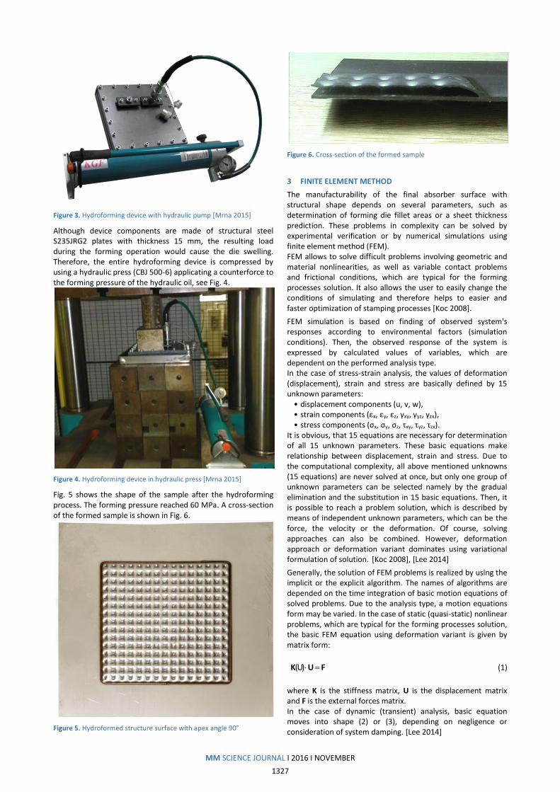
Figure 3. Hydroforming device with hydraulic pump [Mrna 2015]

Although device components are made of structural steel S235JRG2 plates with thickness 15 mm, the resulting load during the forming operation would cause the die swelling. Therefore, the entire hydroforming device is compressed by using a hydraulic press (CBJ 500-6) applicating a counterforce to the forming pressure of the hydraulic oil, see Fig. 4.

Figure 4. Hydroforming device in hydraulic press [Mrna 2015]

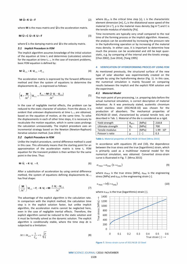
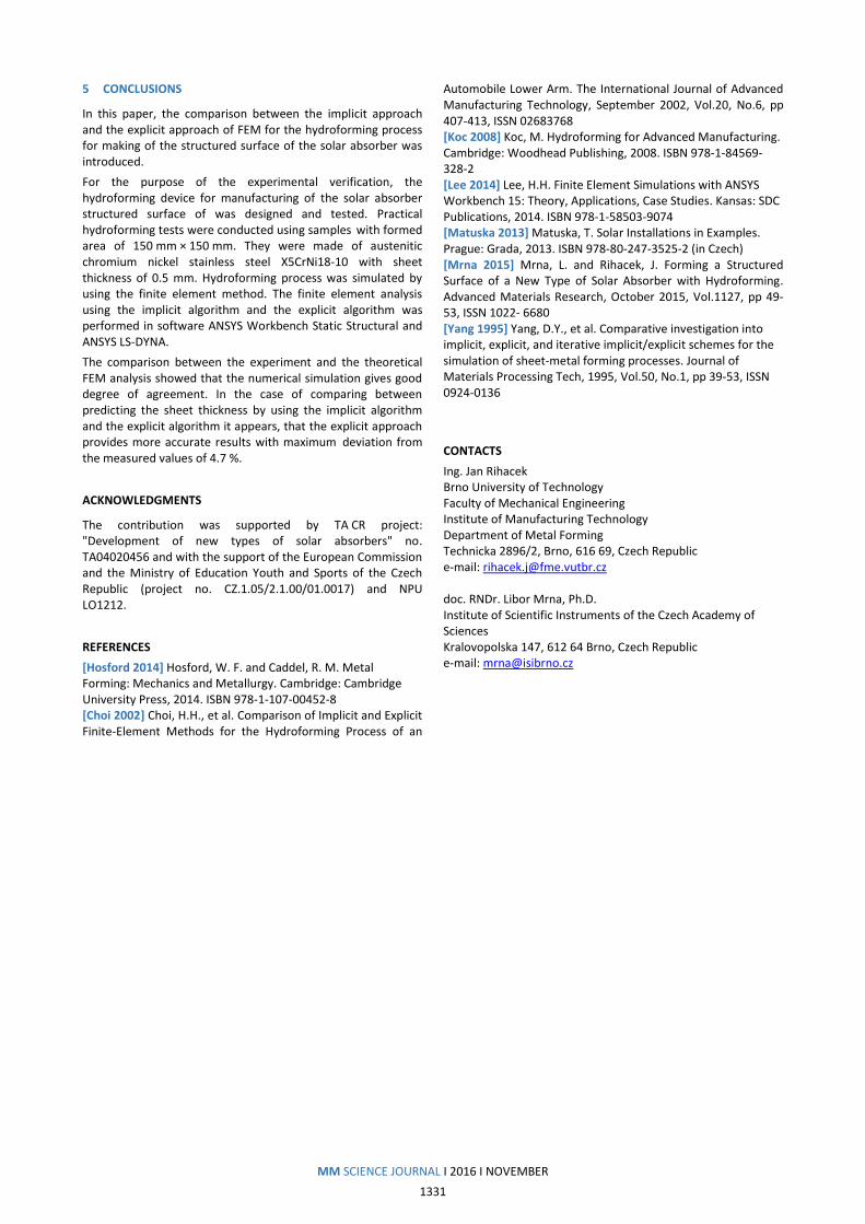
Fig. 5 shows the shape of the sample after the hydroforming process. The forming pressure reached 60 MPa. A cross-section of the formed sample is shown in Fig. 6.

Figure 5. Hydroformed structure surface with apex angle 90°

Figure 6. Cross-section of the formed sample

3 FINITE ELEMENT METHOD

The manufacturability of the final absorber surface with structural shape depends on several parameters, such as determination of forming die fillet areas or a sheet thickness prediction. These problems in complexity can be solved by experimental verification or by numerical simulations using finite element method (FEM). FEM allows to solve difficult problems involving geometric and material nonlinearities, as well as variable contact problems and frictional conditions, which are typical for the forming processes solution. It also allows the user to easily change the conditions of simulating and therefore helps to easier and faster optimization of stamping processes [Koc 2008].

FEM simulation is based on finding of observed system's responses according to environmental factors (simulation conditions). Then, the observed response of the system is expressed by calculated values of variables, which are dependent on the performed analysis type. In the case of stress-strain analysis, the values of deformation (displacement), strain and stress are basically defined by 15 unknown parameters:

• displacement components (u, v, w), • strain components (εx, εy, εz, γxy, γyz, γzx), • stress components (σx, σy, σz, τxy, τyz, τzx).

It is obvious, that 15 equations are necessary for determination of all 15 unknown parameters. These basic equations make relationship between displacement, strain and stress. Due to the computational complexity, all above mentioned unknowns (15 equations) are never solved at once, but only one group of unknown parameters can be selected namely by the gradual elimination and the substitution in 15 basic equations. Then, it is possible to reach a problem solution, which is described by means of independent unknown parameters, which can be the force, the velocity or the deformation. Of course, solving approaches can also be combined. However, deformation approach or deformation variant dominates using variational formulation of solution. [Koc 2008], [Lee 2014]

Generally, the solution of FEM problems is realized by using the implicit or the explicit algorithm. The names of algorithms are depended on the time integration of basic motion equations of solved problems. Due to the analysis type, a motion equations form may be varied. In the case of static (quasi-static) nonlinear problems, which are typical for the forming processes solution, the basic FEM equation using deformation variant is given by matrix form:

FUK )U( (1)

where K is the stiffness matrix, U is the displacement matrix and F is the external forces matrix. In the case of dynamic (transient) analysis, basic equation moves into shape (2) or (3), depending on negligence or consideration of system damping. [Lee 2014]

MM SCIENCE JOURNAL I 2016 I NOVEMBER

1328

FUKUM (2)

where M is the mass matrix and U is the acceleration matrix.

FUKUCUM (3)

where C is the damping matrix and U is the velocity matrix.

3.1 Implicit Procedure in FEM

The implicit algorithm assumes knowledge of the initial solution of the equation at time ti and determines (calculates) solution for the equation at time ti + 1. In the case of transient problems, basic FEM equation is defined by:

1i1i1i FUKUM (4)

The acceleration matrix is expressed by the forward difference method and then the system of equations to determine the displacements Ui + 1 is expressed as follows:

2

1ii1i1i2 t

)2(

t

UUMFU

MK (5)

In the case of negligible inertial effects, the problem can be reduced to the static character of solution. From the above, it is evident that unknown displacements at time ti + 1 are obtained, based on the equation of motion, at the same time. To solve the displacements in each of other time steps, it is necessary to recalculate the motion equation, which in some cases prolongs the calculation unreasonably. The implicit procedure uses an incremental strategy based on the Newton (Newton-Raphson) iterative solution method. [Lee 2014]

3.2 Explicit Procedure in FEM

Unlike the implicit procedure, central difference method is used in this case. This ultimately means that the starting point for an approximation of the acceleration matrix is time ti. FEM equation for the transient problem is then written for the same point in the time. Thus:

iii FUKUM (6)

After a substitution of acceleration by using central difference method, the system of equations defining displacements Ui + 1

has final shape:

2

1iiii1i2 t

2

t

UUMUKFU

M (7)

The advantage of the explicit algorithm is the calculation rate. In comparison with the implicit method, the calculation time step is in the explicit solution faster, but unlike implicit algorithm, the acceleration matrix cannot be neglected here, even in the case of negligible inertial effects. Therefore, the explicit algorithm cannot be reduced to the static solution and it must be formally solved as the dynamic solution. The explicit algorithm is conditionally stable, where the time step Δt is subjected to a limitation:

EL

C

Ltt

dcrit

(8)

where Δtcrit is the critical time step [s], L is the characteristic element dimension [m], Cd is the dilatational wave speed of the material [m∙s-1], ρ is the material mass density [kg∙m-3] and E is the tensile modulus of elasticity [Pa].

Time increments are typically very small compared to the real time of the forming process or the implicit algorithm. However, the analysis can be accelerated by increasing the pressure rate in the hydroforming operation or by increasing of the material mass density. In either case, it is important to determine how much the process can be accelerated and still be kept quasi-static, e.g. by comparing of the internal and the kinetic energy. [Choi 2002], [Lee 2014], [Yang 1995]

4 VERIFICATION OF HYDROFORMING PROCES BY USING FEM

As mentioned previously, the structured surface of the new type of solar absorber was experimentally created on the sample by using the hydroforming device (Fig. 1). In this case, the numerical simulation is mainly focused on comparing results between the implicit and the explicit FEM solution and the experiment.

4.1 Material Model

The main point of pre-processing, i.e. preparing data before the actual numerical simulation, is correct description of material behaviour. As it was previously stated, austenitic chromium nickel stainless steel (X5CrNi18-10) was chosen for the production of absorbers. The mechanical properties of X5CrNi18-10 steel, characterized by uniaxial tensile test, are described in Tab. 1. Material of the die is considered as a rigid.

Yield strength Rp0.2 [MPa] 218.8

Ultimate strength Rm [MPa] 700

Tensile modulus E [MPa] 1.99 ∙ 105

Poisson´s ratio µ [ - ] 0.3

Table 1. Material properties of X5CrNi18-10 Steel [Mrna 2015]

In accordance with equations (9) and (10), the dependence between the true stress and the true (logarithmic) strain, which is primarily used as a multilinear material model for the numerical simulation, was obtained. Converted stress-strain curve is illustrated in Fig. 7. [Mrna 2015]

ENGENGTRUE 1 (9)

where σTRUE is the true stress [MPa], σENG is the engineering stress [MPa] and εENG is the engineering strain [-].

ENGTRUE 1ln (10)

where εTRUE is the true (logarithmic) strain [-].

Figure 7. Stress-strain curve of X5CrNi18-10 Steel

MM SCIENCE JOURNAL I 2016 I NOVEMBER

1329

4.2 Geometrical Model

It is important to note that the simplified geometrical model was used. It is based on a partial symmetry and neglect possibility of those parts that do not have direct involvement in the hydroforming process. Taking into account the symmetry possibilities, a quarter-model was used. The geometrical model was created in software Autodesk Inventor Professional 2016. Then it was imported into the simulation software in *.iges format. The final geometrical model for the numerical simulation is shown in Fig. 8.

Figure 8. Geometrical model of the hydroforming process

Further, it is necessary to make a full continuum discretization of the stamped material and tools by using a finite element mesh. The discretization of a solved continuum was performed with using four-node quadrilateral shell elements. The emphasis was placed on the requirement for the FEM mesh uniformity, mainly due to correctness of results. In the case of the mesh application to the formed sheet, elements with an edge length of 0.5 mm were used.

A fully defined model, which is ready for calculation, was obtained after discretization of individual macro elements and applying boundary conditions, i.e. stamping pressure or contacts. The friction coefficient between the formed sample and the die wall was set at 0.15.

4.3 Computational Model

Two approaches for the solving process were applicated by using different FEM software. For the implicit approach, ANSYS Workbench 16 software, Static Structural module, which is primarily intended to solve static or quasi-static problems, was used. For the explicit approach, ANSYS LS-DYNA R7.1.1 software was used. It should be noted that these programs require different material data.

In the case of ANSYS Workbench Static Structural software, description of an elastic and a plastic behaviour using above mentioned material data is sufficient.

Moreover, the explicit solver requires a density value. The X5CrNi18-10 steel density at 20 °C is 7.9∙103 kg∙m-3. To reduce the time consumed by the calculation, higher density value (7.9∙105 kg∙m-3) was entered into the ANSYS LS-DYNA software. Furthermore, lower value of the simulation time was entered compared with the reality, namely 10 ms. These interventions may affect the correctness of results and therefore the quasi-static behaviour was checked by comparing the kinetic and the internal energy. The global energy evolution of the simulated system can be seen in Fig. 9.

Figure 9. Internal and kinetic energy history for explicit simulation

4.4 Results

The numerical simulation by using the finite element method gives a stamping depth depending on the required pressure as a primary result.

When the forming pressure is set at 60 MPa, the implicit approach gives approximately 3.67 mm as a maximum indents depth. In the same case, the explicit approach shows 3.66 mm. Fig. 10 and Fig. 11 show a prediction of the achievable indents depth without defects, i.e. the hydroformed structure shape using the pressure of 60 MPa, which is predicted by the implicit approach and the explicit approach.

Figure 10. Prediction of indents depth using ANSYS Workbench Static Structural (implicit)

Figure 11. Prediction of indents depth using ANSYS LS-DYNA (explicit)

In order to compare results, which were obtained by the numerical simulation, indents depth measuring of the hydroformed sample was performed. The maximum depth of indents, which was determined on the basis of experimental measurement by using caliper PROTECO, is 3.65 mm. It is the average value of 5 measurements.

MM SCIENCE JOURNAL I 2016 I NOVEMBER

1330

One of the most significant results of the numerical simulation using FEM is also the structured surface thickness analysis of the sample. Results from the implicit approach and the explicit approach were subsequently confronted with an experimental way by indents profile measuring.

The thickness of formed sheet was measured by digital tip micrometer Mitutoyo. With regard to complexity of the structured surface shape, measurement was performed in two directions, i.e. in a straight direction and also in a diagonal direction. Measurements were always carried out from the edge behind the weld bead across three indents. It was performed three times for each direction and a mean values were created. A schematic representation of measurement paths is shown in Fig. 12.

Figure 12. Measurement paths

The hydroforming test evaluation for the direct measurement and for the diagonal measurement is presented in Fig. 13 and in Fig. 14. Variable thickness values can be observed in both groups.

Due to the fact, that the sample final shape is formed at the cost of the sheet thinning, variable values of the structured surface thickness can be observed, i.e. from about 0.49 mm to 0.36 mm, according to detecting methods. Especially, significant thinning on tops of pyramidal indents is particularly evident. A thinning in these cases amounts to 0.14 mm.

From the viewpoint of comparing between simulation results using ANSYS Workbench Static Structural and ANSYS LS-DYNA and experimental measurements, in the case of the diagonal measurement, deviations from the measured values are obvious, especially in the area from the weld to the first indent, i.e. measured distance from 0 mm to 5 mm, see Fig. 13. The largest deviations from the measured values are approximately 4.9 % for the implicit approach and 4.7 % for the explicit approach. In other areas of the graph, especially bottom areas of indents, which are expanded by the fluid pressure to the open space, results show lower agreement degree (measured distance 10 mm and 20 mm).

The calculation by using the implicit approach predicated material thickness, which is 4 % higher than the experimental measurement shows. In contrast, the explicit approach has a very good conformity degree with a maximum deviation of 1.9 %.

Figure 13. Thickness of indents – direct measurement

Similar results were obtained also in the case of the diagonal measurement, see Fig. 14. In terms of agreement, the most problematic area is in measured distance from 0 mm to 7 mm. In a global view, the implicit approach shows greater differences compared to the experimental measured values than the explicit approach. In this case, the highest detected deviation is 7.7 % (measured distance of 4 mm). The maximal deviation at the bottom of indents is then about 6.5 %. Compared with this, the highest difference of 4.6 % was found in the explicit solution. At the bottom of indents is the difference between FEM simulation and the experiment of about 3.3%.

Figure 14. Thickness of indents – diagonal measurement

It is essential to recognize that comparison between the numerical simulation by using ANSYS Workbench Static Structural, respectively ANSYS LS-DYNA and the experimental measurement shows a good level of agreement in results, where maximum deviation between FEM and experimental results is 7.7 % namely in the case of the implicit solution. From the performed comparison is also evident that the explicit approach gives better results, mainly for exposed areas with a high deformation level, where deviations from the experimentally determined values of thickness are insignificant.

MM SCIENCE JOURNAL I 2016 I NOVEMBER

1331

5 CONCLUSIONS

In this paper, the comparison between the implicit approach and the explicit approach of FEM for the hydroforming process for making of the structured surface of the solar absorber was introduced.

For the purpose of the experimental verification, the hydroforming device for manufacturing of the solar absorber structured surface of was designed and tested. Practical hydroforming tests were conducted using samples with formed area of 150 mm × 150 mm. They were made of austenitic chromium nickel stainless steel X5CrNi18-10 with sheet thickness of 0.5 mm. Hydroforming process was simulated by using the finite element method. The finite element analysis using the implicit algorithm and the explicit algorithm was performed in software ANSYS Workbench Static Structural and ANSYS LS-DYNA.

The comparison between the experiment and the theoretical FEM analysis showed that the numerical simulation gives good degree of agreement. In the case of comparing between predicting the sheet thickness by using the implicit algorithm and the explicit algorithm it appears, that the explicit approach provides more accurate results with maximum deviation from the measured values of 4.7 %.

ACKNOWLEDGMENTS

The contribution was supported by TA CR project: "Development of new types of solar absorbers" no. TA04020456 and with the support of the European Commission and the Ministry of Education Youth and Sports of the Czech Republic (project no. CZ.1.05/2.1.00/01.0017) and NPU LO1212.

REFERENCES

[Hosford 2014] Hosford, W. F. and Caddel, R. M. Metal Forming: Mechanics and Metallurgy. Cambridge: Cambridge University Press, 2014. ISBN 978-1-107-00452-8 [Choi 2002] Choi, H.H., et al. Comparison of Implicit and Explicit Finite-Element Methods for the Hydroforming Process of an

Automobile Lower Arm. The International Journal of Advanced Manufacturing Technology, September 2002, Vol.20, No.6, pp 407-413, ISSN 02683768 [Koc 2008] Koc, M. Hydroforming for Advanced Manufacturing. Cambridge: Woodhead Publishing, 2008. ISBN 978-1-84569-328-2 [Lee 2014] Lee, H.H. Finite Element Simulations with ANSYS Workbench 15: Theory, Applications, Case Studies. Kansas: SDC Publications, 2014. ISBN 978-1-58503-9074 [Matuska 2013] Matuska, T. Solar Installations in Examples. Prague: Grada, 2013. ISBN 978-80-247-3525-2 (in Czech) [Mrna 2015] Mrna, L. and Rihacek, J. Forming a Structured Surface of a New Type of Solar Absorber with Hydroforming. Advanced Materials Research, October 2015, Vol.1127, pp 49-53, ISSN 1022- 6680 [Yang 1995] Yang, D.Y., et al. Comparative investigation into implicit, explicit, and iterative implicit/explicit schemes for the simulation of sheet-metal forming processes. Journal of Materials Processing Tech, 1995, Vol.50, No.1, pp 39-53, ISSN 0924-0136

CONTACTS

Ing. Jan Rihacek Brno University of Technology Faculty of Mechanical Engineering Institute of Manufacturing Technology Department of Metal Forming Technicka 2896/2, Brno, 616 69, Czech Republic e-mail: rihacek.j@fme.vutbr.cz doc. RNDr. Libor Mrna, Ph.D. Institute of Scientific Instruments of the Czech Academy of Sciences Kralovopolska 147, 612 64 Brno, Czech Republic e-mail: mrna@isibrno.cz