comparison of geometric integrator...
TRANSCRIPT

COMPARISON OF GEOMETRIC INTEGRATORMETHODS FOR HAMILTON SYSTEMS
A Thesis Submitted tothe Graduate School of Engineering and Sciences of
Izmir Institute of Technologyin Partial Fulfillment of the Requirements for the Degree of
MASTER OF SCIENCE
in Mathematics
byPınar INECI
March 2009IZMIR
We approve the thesis of Pınar INECI
Assoc. Prof. Dr. Gamze TANOGLUSupervisor
Prof. Dr. Oktay PASHAEVCommittee Member
Assist. Prof. Dr. Gurcan ARALCommittee Member
31 March 2009
Prof. Dr. Oguz YILMAZ Prof. Dr. Hasan BOKEHead of the Mathematics Department Dean of the Graduate School of
Engineering and Sciences

ACKNOWLEDGEMENTS
This thesis is the consequence of a three-year study evolved by the contri-
bution of many people and now I would like to express my gratitude to all the
people supporting me from all the aspects for the period of my thesis.
Firstly, I would like to thank and express my deepest gratitude to Assoc.
Prof. Dr. Gamze TANOGLU, my advisor, for her help, guidance, understanding,
encouragement and patience during my studies and preparation of this thesis.
And I would like to thank to TUBITAK for its support.
I also would like to express my special thanks to Engin IZGI for his support,
understanding and love.
Last, thanks to Barıs CICEK, Hakan GUNDUZ and Duygu DEMIR for their
supports. And finally I am also grateful to my family for their confidence to me
and for their endless supports.

ABSTRACT
COMPARISON OF GEOMETRIC INTEGRATOR METHODS FORHAMILTON SYSTEMS
Geometric numerical integration is relatively new area of numerical analy-
sis. The aim of a series numerical methods is to preserve some geometric prop-
erties of the flow of a differential equation such as symplecticity or reversibility.
In this thesis, we illustrate the effectiveness of geometric integration methods.
For this purpose symplectic Euler method, adjoint of symplectic Euler method,
midpoint rule, Stormer-Verlet method and higher order methods obtained by
composition of midpoint or Stormer-Verlet method are considered as geometric
integration methods. Whereas explicit Euler, implicit Euler, trapezoidal rule, clas-
sic Runge-Kutta methods are chosen as non-geometric integration methods. Both
geometric and non-geometric integration methods are applied to the Kepler prob-
lem which has three conserved quantities: energy, angular momentum and the
Runge-Lenz vector, in order to determine which those quantities are preserved
better by these methods.
iv

OZET
HAMILTON SISTEMLER ICIN GEOMETRIK ENTEGRASYONYONTEMLERININ KARSILASTIRILMASI
Geometrik entegrasyon numerik analizin nispeten yeni alanlarından
biridir. Bircok sayısal metodun amacı diferansiyel denklemlerin cozumunun
simplektiklik ya da tersine cevrilebilirlik gibi bazı geometrik ozelliklerini koru-
maktır. Bu tezde geometrik entegrasyon yontemlerinin etkisini ortaya koyduk.
Bu amac dogrultusunda geometrik entegrasyon yontemleri olarak simplektik
Euler metodu, simplektik Euler metodunun adjonti, Stormer-Verlet metod ve
midpoint ya da Stormer-Verlet metodun bileskesi ile elde edilen yuksek mer-
tebeden metodları kullandık. Aynı zamanda Explicit Euler, Implicit Euler, trape-
zoidal rule ve klasik runge-kutta yontemleri geometrik olmayan entegrasyon
yontemleri olarak kullanıldı. Enerji, acısal momentum ve Runge-Lenz vektoru
gibi uc tane korunan, geometrik ozelligi olan kepler problemine, bu ozelliklerin
hangi yontemler tarafından daha iyi korundugunu saptamak icin hem geometrik
hem de geometrik olmayan entegrasyon yontemleri uygulandı.
v

vi
TABLE OF CONTENS
LIST OF FIGURES ........................................................................................................ ix
CHAPTER 1. INTRODUCTION ..................................................................................... 1
CHAPTER 2. PRELIMINARIES..................................................................................... 3
2.1. Introduction to ODEs............................................................................. 4
2.2. The Exact Flow of an ODE.................................................................... 5
2.3. Hamiltonian Systems ............................................................................. 6
CHAPTER 3. NUMERICAL METHODS ....................................................................... 8
3.1. One Step Method ................................................................................... 8
3.2. Derivation of One-step Method ........................................................... 9
3.3. Elementary One Step Method................................................................ 9
3.4. Runge-Kutta Methods.......................................................................... 10
3.5. Partitioned Euler Method..................................................................... 11
3.6. The Störmer-Verlet Scheme ................................................................ 12
3.7. Partitioned Runge-Kutta Methods ....................................................... 13
3.8. Splitting and Composition Methods .................................................... 14
3.9. The Adjoint of a Method...................................................................... 17
CAHPTER 4. CONSERVED QUANTITIES AND GEOMETRIC INTEGRATION...................................................................................... 19
4.1. Exact Conservation of Invariants......................................................... 19
4.1.1. Ouadratic Invariants ...................................................................... 21
4.2. Symplectic Transformations ............................................................... 23
4.3. Examples of Symplectic Integrators .................................................... 26
4.4. Symplectic Runge-Kutta Methods ....................................................... 27
4.5. Examples of Applications of Symplectic Integrators .......................... 29
4.6. Symmetric Integration and Reversibility ............................................. 32

vii
4.6.1. Reversible Differential Equations and Maps ................................ 32
4.7. Examples of Symmetric Methods........................................................ 36
4.8. Geometric Structures in Hamiltonian Systems .................................... 36
4.9. Geometric Integration .......................................................................... 37
4.9.1. Philosopy of Geometric Integration .............................................. 38
4.10. The Kepler Problem and Its Conserved Quantities............................ 40
CHAPTER 5. A COMPARISION OF SYMPLECTIC AND NON-SYMPLECTIC METHODS APPLIED TO KEPLER PROBLEM.............................................................................................. 43
5.1. First Order Methods............................................................................. 43
5.1.1. Phase Spaces ................................................................................. 43
5.1.2. Conservation of Energy................................................................. 46
5.1.3. Conservation of Angular Momentum ........................................... 48
5.1.4. Conservation of Runge-Lenz Vector ............................................ 50
5.2. Second Order Methods ........................................................................ 52
5.2.1. Phase Spaces ................................................................................. 52
5.2.2. Conservation of Energy................................................................. 54
5.2.3. Conservation of Angular Momentum ........................................... 56
5.2.4. Conservation of Runge-Lenz Vector ............................................ 58
5.3. Third Order Methods ........................................................................... 60
5.3.1. Phase Spaces ................................................................................. 60
5.3.2. Conservation of Energy................................................................. 62
5.3.3. Conservation of Angular Momentum ........................................... 64
5.3.4. Conservation of Runge-Lenz Vector ............................................ 66
5.4. Fourth and Fifth Order Methods .......................................................... 68
5.4.1. Phase Spaces ................................................................................. 68
5.4.2. Conservation of Energy................................................................. 70

viii
5.4.3. Conservation of Angular Momentum ........................................... 72
5.4.4. Conservation of Runge-Lenz Vector ............................................ 74
CHAPTER 6. SUMMARY AND CONCLUSION ........................................................ 76
REFERENCES ............................................................................................................... 79
APPENDICES
APPENDICES A. MATLAB CODES ........................................................................... 80
A.1. First Order Methods...................................................................... 80
A.1.1. Explicit Euler ......................................................................... 82
A.1.2. Implicit Euler ......................................................................... 83
A.1.3. Adjoint of Symplectic Euler .................................................. 85
A.2. Second Order Methods ................................................................. 87
A.2.1. Trapezoidal Rule.................................................................... 87
A.2.2. Midpoint Rule........................................................................ 89
A.2.3. Störmer-Verlet Method.......................................................... 91
A.3. Second Order Methods ................................................................. 93
A.3.1. Third Order Runge-Kutta Method ......................................... 93
A.3.2. Composition Method of Order 3 (Midpoint as base method).................................................... 94
A.3.3. Composition Method of Order 3 ( Störmer-Verlet as base method).................................................................................. 99
A.4. Fourth and Fifth Order Methods ................................................. 102
A.4.1. Fourth Order Runge-Kutta Method ..................................... 102
A.4.2. Composition Method of Order 5 (Midpoint as base method)104
A.4.3. Composition Method of Order 5 (Störmer-Verlet as base method)............................................................................... 110
LIST OF FIGURES
Figure Page
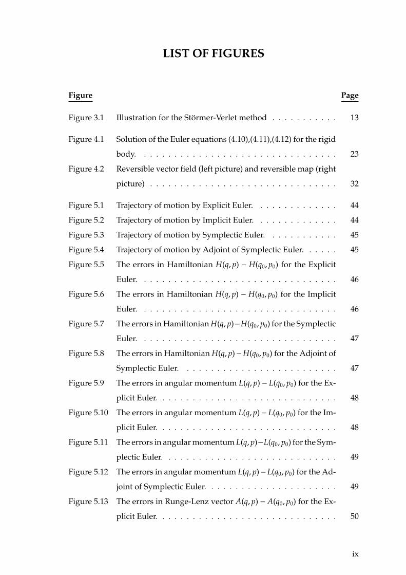
Figure 3.1 Illustration for the Stormer-Verlet method . . . . . . . . . . . 13
Figure 4.1 Solution of the Euler equations (4.10),(4.11),(4.12) for the rigid
body. . . . . . . . . . . . . . . . . . . . . . . . . . . . . . . . . 23
Figure 4.2 Reversible vector field (left picture) and reversible map (right
picture) . . . . . . . . . . . . . . . . . . . . . . . . . . . . . . . 32
Figure 5.1 Trajectory of motion by Explicit Euler. . . . . . . . . . . . . . 44
Figure 5.2 Trajectory of motion by Implicit Euler. . . . . . . . . . . . . . 44
Figure 5.3 Trajectory of motion by Symplectic Euler. . . . . . . . . . . . 45
Figure 5.4 Trajectory of motion by Adjoint of Symplectic Euler. . . . . . 45
Figure 5.5 The errors in Hamiltonian H(q, p) − H(q0, p0) for the Explicit
Euler. . . . . . . . . . . . . . . . . . . . . . . . . . . . . . . . . 46
Figure 5.6 The errors in Hamiltonian H(q, p) − H(q0, p0) for the Implicit
Euler. . . . . . . . . . . . . . . . . . . . . . . . . . . . . . . . . 46
Figure 5.7 The errors in Hamiltonian H(q, p)−H(q0, p0) for the Symplectic
Euler. . . . . . . . . . . . . . . . . . . . . . . . . . . . . . . . . 47
Figure 5.8 The errors in Hamiltonian H(q, p)−H(q0, p0) for the Adjoint of
Symplectic Euler. . . . . . . . . . . . . . . . . . . . . . . . . . 47
Figure 5.9 The errors in angular momentum L(q, p) − L(q0, p0) for the Ex-
plicit Euler. . . . . . . . . . . . . . . . . . . . . . . . . . . . . . 48
Figure 5.10 The errors in angular momentum L(q, p)− L(q0, p0) for the Im-
plicit Euler. . . . . . . . . . . . . . . . . . . . . . . . . . . . . . 48
Figure 5.11 The errors in angular momentum L(q, p)−L(q0, p0) for the Sym-
plectic Euler. . . . . . . . . . . . . . . . . . . . . . . . . . . . . 49
Figure 5.12 The errors in angular momentum L(q, p)−L(q0, p0) for the Ad-
joint of Symplectic Euler. . . . . . . . . . . . . . . . . . . . . . 49
Figure 5.13 The errors in Runge-Lenz vector A(q, p) − A(q0, p0) for the Ex-
plicit Euler. . . . . . . . . . . . . . . . . . . . . . . . . . . . . . 50
ix

Figure 5.14 The errors in Runge-Lenz vector A(q, p) − A(q0, p0) for the Im-
plicit Euler. . . . . . . . . . . . . . . . . . . . . . . . . . . . . . 50
Figure 5.15 The errors in Runge-Lenz vector A(q, p)−A(q0, p0) for the Sym-
plectic Euler. . . . . . . . . . . . . . . . . . . . . . . . . . . . . 51
Figure 5.16 The errors in Runge-Lenz vector A(q, p)−A(q0, p0) for the Ad-
joint of Symplectic Euler. . . . . . . . . . . . . . . . . . . . . . 51
Figure 5.17 Trajectory of motion by Trapezoidal Rule. . . . . . . . . . . . 52
Figure 5.18 Trajectory of motion by Midpoint Rule. . . . . . . . . . . . . . 53
Figure 5.19 Trajectory of motion by Stormer-Verlet scheme. . . . . . . . . 53
Figure 5.20 The errors in Hamiltonian H(q, p)−H(q0, p0) for the Trapezoidal
Rule. . . . . . . . . . . . . . . . . . . . . . . . . . . . . . . . . . 54
Figure 5.21 The errors in Hamiltonian H(q, p) −H(q0, p0) for Midpoint Rule. 55
Figure 5.22 The errors in Hamiltonian H(q, p)−H(q0, p0) for Stormer-Verlet
scheme. . . . . . . . . . . . . . . . . . . . . . . . . . . . . . . . 55
Figure 5.23 The errors in angular momentum L(q, p) − L(q0, p0) for Trape-
zoidal rule. . . . . . . . . . . . . . . . . . . . . . . . . . . . . . 56
Figure 5.24 The errors in angular momentum L(q, p) − L(q0, p0) Midpoint
Rule. . . . . . . . . . . . . . . . . . . . . . . . . . . . . . . . . . 57
Figure 5.25 The errors in angular momentum L(q, p)−L(q0, p0) for Stormer-
Verlet scheme. . . . . . . . . . . . . . . . . . . . . . . . . . . . 57
Figure 5.26 The errors in Runge-Lenz vector A(q, p) − A(q0, p0) for the
Trapezoidal rule. . . . . . . . . . . . . . . . . . . . . . . . . . . 58
Figure 5.27 The errors in Runge-Lenz vector A(q, p)−A(q0, p0) for Midpoint
Rule. . . . . . . . . . . . . . . . . . . . . . . . . . . . . . . . . . 59
Figure 5.28 The errors in Runge-Lenz vector A(q, p)−A(q0, p0) for Stormer-
Verlet scheme. . . . . . . . . . . . . . . . . . . . . . . . . . . . 59
Figure 5.29 Trajectory of motion by 3rd order Runge-Kutta. . . . . . . . . 60
Figure 5.30 Trajectory of motion by Composition method of order 3 (mid-
point rule as base method) . . . . . . . . . . . . . . . . . . . . 61
Figure 5.31 Trajectory of motion by Composition method of order 3
(Stormer-Verlet as base method) . . . . . . . . . . . . . . . . . 61
x

Figure 5.32 The errors in Hamiltonian H(q, p) − H(q0, p0) for 3rd order
Runge-Kutta. . . . . . . . . . . . . . . . . . . . . . . . . . . . . 62
Figure 5.33 The errors in Hamiltonian H(q, p) −H(q0, p0) for Composition
method of order 3 (midpoint rule as base method). . . . . . . 63
Figure 5.34 The errors in Hamiltonian H(q, p) −H(q0, p0) for Composition
method of order 3 (Stormer-Verlet as base method) . . . . . . 63
Figure 5.35 The errors in angular momentum L(q, p)−L(q0, p0) for 3rd order
Runge-Kutta. . . . . . . . . . . . . . . . . . . . . . . . . . . . . 64
Figure 5.36 The errors in angular momentum L(q, p) − L(q0, p0) Composi-
tion method of order 3 (midpoint rule as base method) . . . . 65
Figure 5.37 The errors in angular momentum L(q, p) − L(q0, p0) Composi-
tion method of order 3 (Stormer-Verlet as base method) . . . 65
Figure 5.38 The errors in Runge-Lenz vector A(q, p)−A(q0, p0) for 3rd order
Runge-Kutta . . . . . . . . . . . . . . . . . . . . . . . . . . . . 66
Figure 5.39 The errors in Runge-Lenz vector A(q, p)−A(q0, p0) for Compo-
sition method of order 3 (midpoint rule as base method) . . . 67
Figure 5.40 The errors in Runge-Lenz vector A(q, p)−A(q0, p0) for Compo-
sition method of order 3 (Stormer-Verlet as base method) . . 67
Figure 5.41 Trajectory of motion by 4th order Runge-Kutta. . . . . . . . . 68
Figure 5.42 Trajectory of motion by Composition method of order 5 (mid-
point rule as base method) . . . . . . . . . . . . . . . . . . . . 69
Figure 5.43 Trajectory of motion by Composition method of order 5
(Stormer-Verlet as base method) . . . . . . . . . . . . . . . . . 69
Figure 5.44 The errors in Hamiltonian H(q, p) − H(q0, p0) for 4th order
Runge-Kutta . . . . . . . . . . . . . . . . . . . . . . . . . . . . 70
Figure 5.45 The errors in Hamiltonian H(q, p) −H(q0, p0) for Composition
method of order 5 (midpoint rule as base method) . . . . . . 71
Figure 5.46 The errors in Hamiltonian H(q, p) −H(q0, p0) for Composition
method of order 5 (Stormer-Verlet as base method) . . . . . . 71
Figure 5.47 The errors in angular momentum L(q, p)−L(q0, p0) for 4th order
Runge-Kutta . . . . . . . . . . . . . . . . . . . . . . . . . . . . 72
xi

Figure 5.48 The errors in angular momentum L(q, p) − L(q0, p0) Composi-
tion method of order 5 (midpoint rule as base method) . . . . 73
Figure 5.49 The errors in angular momentum L(q, p) − L(q0, p0) Composi-
tion method of order 5 (Stormer-Verlet as base method) . . . 73
Figure 5.50 The errors in Runge-Lenz vector A(q, p)−A(q0, p0) for 4th order
Runge-Kutta . . . . . . . . . . . . . . . . . . . . . . . . . . . . 74
Figure 5.51 The errors in Runge-Lenz vector A(q, p)−A(q0, p0) for Compo-
sition method of order 5 (midpoint rule as base method) . . . 75
Figure 5.52 The errors in Runge-Lenz vector A(q, p)−A(q0, p0) for Compo-
sition method of order 5 (Stormer-Verlet as base method) . . 75
Figure 6.1 Errors for energy versus time step h in logarithmic scale for
composition method of order 3 (midpoint rule as the base
method) . . . . . . . . . . . . . . . . . . . . . . . . . . . . . . . 78
xii

CHAPTER 1
INTRODUCTION
The topic of this thesis is geometric structure-preserving numerical inte-
gration method for ordinary differential equations. We will concentrate mainly on
Hamiltonian equations and numerical methods that preserve geometric structures
of them.
During the past decade there has been an increasing interest in studying
numerical methods that preserve certain properties of some differential equations
(Budd and Piggott 2000). The reason is that some physical systems possess con-
served quantities, and that the solutions of the systems also should contain these
invariants. Typical examples are the symplectic structure in a Hamiltonian sys-
tem, the energy in a conservative mechanical system and the angular momentum
of a rotating rigid body in space. Classical numerical methods normally fail to
preserve such as the above mentioned quantities (Budd and Piggott 2000).
Frequently we need to integrate numerically a system of ordinary differen-
tial equations (ODEs) having some first integrals or admitting some conservation
laws. In what follows we will consider exclusively the ODE case, but our method
can also be applied to the case of partial differential equations. Many examples of
systems of ODEs having first integrals can be found in classical mechanics, where
Hamiltonian equations are of this type, always having the Hamiltonian as a first
integral.
In this thesis we mainly concern with symplectic geometric integration
methods. We will give the definition of symplectic maps, and call any numerical
scheme which induces a symplectic map as the symplectic numerical method.
For numerical implementation we choose the Kepler problem. Conserved
quantities of the Kepler problem are the energy, the angular momentum and the
Runge-Lenz vector. We applied both geometric and non-geometric integration
methods to the Kepler problem. We observed that symplectic methods were
most successful. We illustrate the effectiveness of geometric integration methods,
namely symplectic Euler, adjoint of symplectic Euler, midpoint rule and Stormer-
1

Verlet method which is composition of symplectic Euler and its adjoint. In this
study third and fifth order methods are constructed by composition techniques
by considering midpoint rule and Stormer-Verlet method as base method. For
comparison reason non-symplectic methods are also chosen.
The outline of this thesis as follows: After giving some preliminaries in
Chapter 2, geometric numerical methods and non-geometric methods that we
use in our computations are introduced in Chapter 3. And we discuss some
geometric properties, first integrals of the differential equations and philosophy
of geometric integration in Chapter 4. Finally; both geometric and non-geometric
methods, that we introduce in Chapter 4, are applied to the Kepler problem in
Chapter 5, in order to see advantages and disadvantages of geometric integration.
2

CHAPTER 2
PRELIMINARIES
This chapter consist of some preliminary information about geometric in-
tegration method. We introduce the exact flow of an ODE and general properties
of exact flows. We also give the definition of an integrator and some properties of
integrators. Also a brief discussion is given on the geometric integration method
idea. Finally we introduce the Hamiltonian systems.
The motion is described by differential equations, which are derived from
the laws of physics. These equations contain within them not just a statement
of the current acceleration experienced by the object(s), but all the physical laws
relevant to the particular situation. Finding these laws and their consequences
for the motion has been a major part of physics since the time of Newton (Stuart
and Humphries 1996). For example, the equations tell us the space in which
the system evolves (its phase space, which may be ordinary Euclidean space or a
curved space such as a sphere); any symmetries of the motion, such as left-right
or forward-backward symmetries of a pendulum; and any special quantities such
as energy, which for a pendulum is either conserved. Most importantly, the laws
describe how all motion starting close to the actual one are constrained in relation
to each other. These laws are known as symplecticity and volume preservation
(Stuart and Humphries 1996).
Standard methods for simulating motion, called numerical integrators,
take an initial condition and move the objects in direction specified by the differ-
ential equations. They completely ignore all of the above hidden physical laws
contained within the equations. Since about 1990, new methods have been devel-
oped, called geometric integrators, which obey these extra laws (Budd and Iserles
1999). Since the methods are physically natural, we can hope that the results will
be extremely reliable, especially for long-time simulations. Before we list you
advantages of the method, we mention three disadvantages:
• The hidden physical law usually has to be known if the integrator is going
to obey it. For example to preserve energy, the energy must be known.
3
• Because we are asking something more in this method, it may turn out to
be computationally more expensive then a standard method. Amazingly
(because the laws are so natural) sometimes it’s actually much cheaper.
• Many systems have several hidden laws, but the methods currently known
preserve one of them but not all simultaneously (Quispel and Dyt 1997).
Now the advantages of the method:
• Simulations can be run for enormously long times, because there are no
spurious non-physical effects, such as dissipation of energy in a conservative
system.
• By studying structure of the equations, very simple, fast, and reliable geo-
metric integrators can often be found;
• In some situations, results can be guaranteed to be qualitatively correct, even
when the motion is chaotic.
• For some systems, for short, medium and long times even the actual quan-
titative errors are much smaller than in standard methods (Quispel and Dyt
1997).
2.1. Introduction to ODEs
Coming from classical mechanics ordinary differential equations (ODEs)
were developed to model mechanical systems. Most dynamical systems -physical,
biological, engineering- are often conveniently expressed in the form of differential
equations.
Let R be the set of all real numbers and I be an open interval on the real
line R, that is, I = {t : t ∈ R, r1 < t < r2}, where r1, r2 are any two fixed points
in R. Also, let Rn denote the real n-dimensional Euclidean space with elements
x = (x1, x2, ..., xn), and letRn+1 be the space of elements of (n+1)-tuple (t, x1, x2, ..., xn)
or (t, x). Let B be a domain, i.e, an open-connected set in Rn+1, and C[B,Rn] be a
class of functions defined and continuous on B.
An ordinary differential equation of the n-th order and of the form
F(t,u,u′,u′′, ..., u(n)) = 0 (2.1)
4

where u(n) is the n-th derivative of the unknown function u with respect to t and F
is defined in some subset of Rn+2, express a relation between the (n+2)-variables
t,u,u′,u′′, ..., u(n) (Rao 1979).
System of Differential Equations
We shall consider a system of differential equations of the form
u′1 = f1(t,u1, ..., un)
u′2 = f2(t,u1, ..., un)
.
.
.
u′n = fn(t,u1, ..., un)
In vector notation, these equations can be written as
u′ = f (t,u) (2.2)
where u = (u1,u2, ..., un), f = ( f1, f2, ..., fn) are vectors in Rn. We shall assume that
f ∈ C[B,Rn]. With an initial condition
u(t0) = u0 (2.3)
where u0 = (u10,u20, ..., un0) is a vector in Rn. Relations (2.2) and (2.3) constitute a
so-called initial value problem (IVP) (Rao 1979). A set of n-functions φ1, φ2, ..., φn
defined on I is said to be solution of IVP if, for t ∈ I,
� φ′1(t), ..., φ′n(t) exist,
� the point (t, φ1(t), ..., φn(t)) remains in B,
� φ′i(t) = fi(t, φ1(t), ..., φn(t)), i = 1, 2, ..., n
� φi(t0) = φi0, i = 1, 2, ..., n
2.2. The Exact Flow of an ODE
We first define the exact flow (or solution) of an ordinary differential equa-
tion and discuss what properties one would like an integrator to have. Let u(t) be
the exact solution of the system of ordinary equations (ODEs)
dudt
= f (u(t)), u(t0) = u0, u(t) ∈ Rn (2.4)
5
the exact flow ϕh is defined by
u(t + h) = ϕh(u(t)) ∀t, h ∈ R
For each fixed time step h, ϕ is a map from the phase space to itself,i.e, ϕh : Rn →Rn.
2.3. Hamiltonian Systems
In this section we give the definition of the Hamiltonian system.
Definition 2.1 Suppose that H(q,p) is a smooth function of its arguments for
q and p ∈ Rn. Then the dynamical system:
qi =∂H∂pi
(2.5)
pi = −∂H∂qi
(2.6)
(i = 1,2,...,n) is called a Hamiltonian system and H is the Hamiltonian function (or just
the Hamiltonian) of the system. Equations (2.5) and (2.6) called Hamiltons equations.
Definition 2.2 The number of degrees of freedom of a Hamiltonian system is the number
of (qi, pi) pairs in Hamilton’s equations, i.e. the value of n.
In mechanics, the vector q represents the generalized coordinates of the
components of the system (positions, angles, etc.), while p is a set of generalized
momenta. Note that the Hamiltonian function is a constant of the motion:
dHdt
=
n∑
i=1
∂H∂qi
qi +∂H∂pi
pi
=
n∑
i=1
∂H∂qi
∂H∂pi
+∂H∂pi
(−∂H∂qi
) = 0
Example 2.1 A harmonic oscillator is a mass-spring system with potential energy 12kq2,
where q is the displacement of the spring from equilibrium. For simple systems like this
one, in which the potential energy simply depends on the position, the Hamiltonian is just
the total energy:
H(q, p) =12
kq2 +p2
2m(2.7)
6
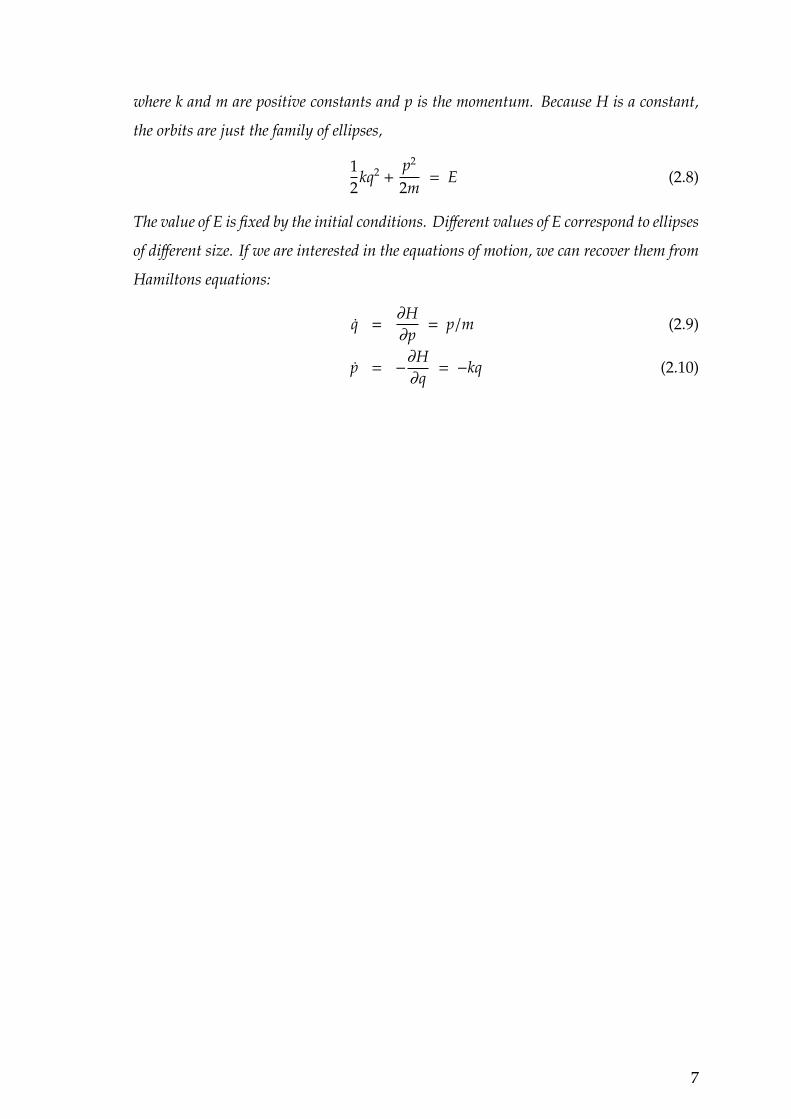
where k and m are positive constants and p is the momentum. Because H is a constant,
the orbits are just the family of ellipses,
12
kq2 +p2
2m= E (2.8)
The value of E is fixed by the initial conditions. Different values of E correspond to ellipses
of different size. If we are interested in the equations of motion, we can recover them from
Hamiltons equations:
q =∂H∂p
= p/m (2.9)
p = −∂H∂q
= −kq (2.10)
7

CHAPTER 3
NUMERICAL METHODS
In this chapter, we introduce numerical methods approximating the solu-
tion of initial value problem for ordinary differential equation.
ddt
y = f (y), y(t0) = y0 ∈ Rk. (3.1)
Here y(t) represents the solution at a particular time t; y = y(t) thus defines a
parameterized trajectory in Rk. We assume that trajectories are defined for all
initial values y0 ∈ Rn and for all times t ≥ t0. For simplicity, we typically take
t0 = 0. One also often uses the notation y(t; y0) to distinguish the trajectory for
a given initial value y0. Define a mapping, or rather a one-parametric family of
mappings, {φt}t≥0, which take initial data to later points along trajectories, i.e.
φt(y0) = y(t; y0), y0 ∈ Rk
A numerical method for solving ordinary differential equations is a map-
ping Φh defined on the phase space that approximates the time-h flow ϕh; if
Φh(y) = ϕh(y) + O(hr+1). The numerical approximation at time t = nh is obtained
by yn = Φh(yn−1) (Budd and Iserles 1999).
3.1. One Step Method
We will primarily concerned with the generalized one-step method. By
iterating the flow map, we know that we obtain a series of snapshots of the true
trajectory
y0, φ∆t(y0), φ∆t ◦ φ∆t(y0), ...
or, compactly, {φn∆t(y0)}∞n=0, where the composition powerφn
∆t is the identity if n = 0
and is otherwise the n-fold composition of φ∆t with itself. For a one-step method,
the approximating trajectory can be viewed as the iteration of another mapping
ψ∆t = Rk → Rk of the underlying space, so that
yn = ψn∆t(y0). (3.2)
8

The mapping ψ∆t is generally nonlinear, will depend on the function f and/or
derivatives, and may be quite complicated, because one-step method generate a
mapping of the phase space (Leimkuhler and Reich 2004).
3.2. Derivation of One-step Method
One step method can be derived in various ways. One way is first to
integrate both sides of ddt y = f (y) on a small interval [t, t + ∆t], obtaining
y(t + ∆t) − y(t) =
∫ ∆t
0f (y(t + τ))dτ.
The right-hand side can then be replaced by a suitable quadrature formula result-
ing in an approximation of the form
y(t + ∆t) ≈ y(t) +
s∑
i=1
bi f (y(t + τi))
for an appropriate set of weights {bi} and quadrature points {τi} (Leimkuhler and
Reich 2004).
3.3. Elementary One Step Method
In this section we will introduce elementary one-step methods.
Explicit Euler Method:
yn+1 = yn + ∆t f (yn)
the quadrature rule used is just∫ ∆t
0f (y(t + τ))dτ = ∆t f (y(t)) + O(∆t2)
Implicit Euler Method:
yn+1 = yn + ∆t f (yn+1)
Trapezoidal Rule:
yn+1 = yn +∆t2
[ f (yn) + f (yn+1)]
the trapezoidal rule is based on∫ ∆t
0f (y(t + τ))dτ =
12
∆t[ f (y(t)) + f (y(t + ∆t))] + O(∆t3)
9

Implicit Midpoint Method:
yn+1 = yn + ∆t f( yn + yn+1
2
)
the quadrature rule is defined as∫ ∆t
0f (y(t + τ))dτ = ∆t f
(y(t) + y(t + ∆t)2
)+ O(∆t3)
3.4. Runge-Kutta Methods
All of the methods discussed so far are special cases of Runge-Kutta meth-
ods. We treat non-autonomous systems of first order ordinary differential equa-
tions
y = f (t, y) y(t0) = y0 (3.3)
Let bi, ai j (i, j = 1, ..., s) be real numbers and let ci =∑s
j=1 ai j. An s − stage Runge −Kutta method is given by
ki = f (t0 + cih, y0 + hs∑
j=1
ai jk j), i = 1, ..., s (3.4)
y1 = y0 + hs∑
i=1
biki (3.5)
Here we allow a full matrix (ai j) of non-zero coefficients. In this case, the slopers
ki can no longer be computed explicitly, and even do not necessarily exist(Hairer,
et al. 2001).
In Butcher tableau the coefficients are usually displayed as follows:
c1 a11 . . . a1s
. . .
. . .
. . .
cs as1 . . . ass
b1 . . . bs
The number of stages s and the constant coefficients {bi},{ai j} completely charac-
terize a Runge-Kutta method. In general, such a method is implicit and leads to a
10

nonlinear system in the s internal stage variables yn. An example of a fourth-order
explicit Runge-Kutta method is given (Butcher 1987).
Let an initial value problem be specified as follows:
y = f (t, y) y(t0) = y0 (3.6)
Then, the RK4 method for this problem is given by the following equations:
yn+1 = yn +16
h(k1 + 2k2 + 2k3 + k4) (3.7)
tn+1 = tn + h (3.8)
where yn+1 is the RK4 approximation o f y(tn+1) and
k1 = f (tn, yn)
k2 = f (tn +12
h, yn +12
hk1)
k3 = f (tn +12
h, yn +12
hk2)
k4 = f (tn +12
h, yn +12
hk3)
3.5. Partitioned Euler Method
For partitioned systems
u = a(u, v), (3.9)
v = b(u, v),
such as the Lotka-Volterra problem we consider also partitioned Euler methods
un+1 = un + ha(un, vn+1) (3.10)
vn+1 = vn + hb(un, vn+1) (3.11)
which treat one variable by the implicit and the other variable by the explicit
Euler method. In view of an important property of this method, discovered by de
Vogelaere (1956) and we call them symplectic Euler methods if we apply the method
to Hamiltonian systems (Hairer 2005).
11
3.6. The Stormer-Verlet Scheme
The equations for the pendulum are of the form
p = f (q) (3.12)
q = p
or
q = f (q)
which is the important special case of a second order differential equation. The
most natural discretisation of (3.12) is
qn+1 − 2qn + qn−1 = h2 f (qn), (3.13)
which is just obtained by replacing the second derivative in (3.12) by the central
second-order difference quotient. This basic method, or its equivalent formulation
given below, is called the Stormer method in astronomy, the Verlet method in molec-
ular dynamics, the leap-frog method in the context of partial differential equations,
and it has further names in other areas. Stormer(1907) used higher-order variants
for numerical computations in molecular dynamics, where it has become by far
the widely used integration scheme (Hairer 2005).
Geometrically, the Stormer-Verlet method can be seen as produced by
parabolas, which in the points tn possess the right second derivative f (qn). But
we can also think of polygons, which possess the right slope in the midpoints
(Figure(3.1) to the right).
Approximations to the derivative p = q are simply obtained by
pn =qn+1 − qn−1
2hand pn+1/2 =
qn+1 − qn
h
One step formulation: The Stormer-Verlet method admits one-step formulation
which is useful for actual computations. The value qn together with the slope pn
and the second derivative f (qn), all at tn, uniquely determine the parabola and
hence also the approximation (pn+1, qn+1) at tn+1. Writing (3.13) as pn+1/2 − pn−1/2 =
h f (qn)) and using pn+1/2 + pn−1/2 = 2pn, we get by elimination of either pn+1/2 or
12
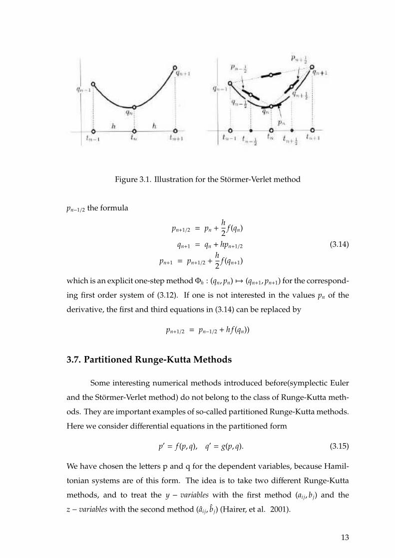
Figure 3.1. Illustration for the Stormer-Verlet method
pn−1/2 the formula
pn+1/2 = pn +h2
f (qn)
qn+1 = qn + hpn+1/2 (3.14)
pn+1 = pn+1/2 +h2
f (qn+1)
which is an explicit one-step method Φh : (qn, pn) 7→ (qn+1, pn+1) for the correspond-
ing first order system of (3.12). If one is not interested in the values pn of the
derivative, the first and third equations in (3.14) can be replaced by
pn+1/2 = pn−1/2 + h f (qn))
3.7. Partitioned Runge-Kutta Methods
Some interesting numerical methods introduced before(symplectic Euler
and the Stormer-Verlet method) do not belong to the class of Runge-Kutta meth-
ods. They are important examples of so-called partitioned Runge-Kutta methods.
Here we consider differential equations in the partitioned form
p′ = f (p, q), q′ = g(p, q). (3.15)
We have chosen the letters p and q for the dependent variables, because Hamil-
tonian systems are of this form. The idea is to take two different Runge-Kutta
methods, and to treat the y − variables with the first method (ai j, b j) and the
z − variables with the second method (ai j, b j) (Hairer, et al. 2001).
13
Definition 3.1 Let bi; ai j and bi; ai j be the coefficients of two Runge-Kutta methods. A
partitioned Runge-Kutta method is given by
ki = f (p0 + hS∑
j=1
ai jk j, q0 + hS∑
j=1
ai j` j)
`i = g(p0hS∑
j=1
ai jk j, q0 + hS∑
j=1
ai j` j) (3.16)
p1 = p0 + hS∑
i=1
biki, q1 = q0 + hS∑
i=1
bi`i
Methods of this type have originally been proposed by Hofer (1976) and Griepen-
trog (1978). Their importance for Hamiltonian systems has been discovered only
very recently.
An interesting example is the partitioned Euler method (3.9-3.11), where
the implicit Euler method b1 = 1, a11 = 1 is combined with the explicit Euler
method b1 = 1, a11 = 0. The Stormer-Verlet method (3.14) is of the form (3.16) with
coefficients given in below table
0 0 0
1 1/2 1/2
1/2 1/2
1/2 1/2 0
1/2 1/2 0
1/2 1/2
The theory of Runge-Kutta methods can be extended in a straight-forward way
to partitioned methods. Since equation (3.16) is a one-step method (p1, q1) =
Φh(p0, q0), the order, the adjoint method and symmetric methods are defined in
the usual way (Hairer, et al. 2001).
3.8. Splitting and Composition Methods
These methods exploit natural decompositions of the problems and partic-
ular of the Hamiltonian and have been used with great success in studies of the
solar system and of molecular dynamics. Much recent work in this field is due to
Yoshida and McLachlan (Budd and Piggott 2000). The main idea behind splitting
methods is to decompose the discrete flow Ψh as a composition of simpler flows
Ψh = Ψ1,h ◦Ψ2,h ◦Ψ3,h...,
14

where each of the sub-flows is chosen such that each represent a simpler integra-
tion of the original. A geometrical perspective on this approach is to find useful
geometric properties of each of the individual operations which are preserved
under combination, symplecticity is just such a property, but we often seek to
preserve reversibility and other structures. Suppose that a differential equation
takes the form
dudt
= f = f1 + f2 (3.17)
Here the functions f1 and f1 may well represent different physical processes in
which case there is a natural decomposition of the problem (say into terms to
kinetic and potential energy).
The most direct form of splitting methods decompose this equation into two
problems
du1
dt= f1 and
du2
dt= f2 (3.18)
chosen such that these two problems can be integrated exactly in closed form to
give explicitly computable flows Ψ1(t) and Ψ2(t). We denote by Ψi,h the result of
applying the corresponding continuous flows ψi(t) over a time h. A simple (first
order) splitting is then given by the Lie-Trotterr formula
Ψh = Ψ1,h ◦Ψ2,h
Suppose that the original problem has Hamiltonian H = H1 +H2, then as observed
earlier this is the composition of two problems with respective Hamiltonian H1
and H2. The differential equation corresponding to each Hamiltonian leads to an
evolutionary map ψi(t) of the form described above.
The Lie-Trotter splitting introduces local errors proportional to h2 at each step and
a more accurate decomposition is the Strang splitting given by
Ψh = Ψ1,h/2 ◦Ψ2,h ◦Ψ1,h/2.
This splitting method has a local error proportional to h3 (Budd and Piggott 2000).
Example 3.1 Suppose that a Hamiltonian system has a Hamiltonian which can be ex-
pressed as a combination of a kinetic energy and a potential energy term as follows
15
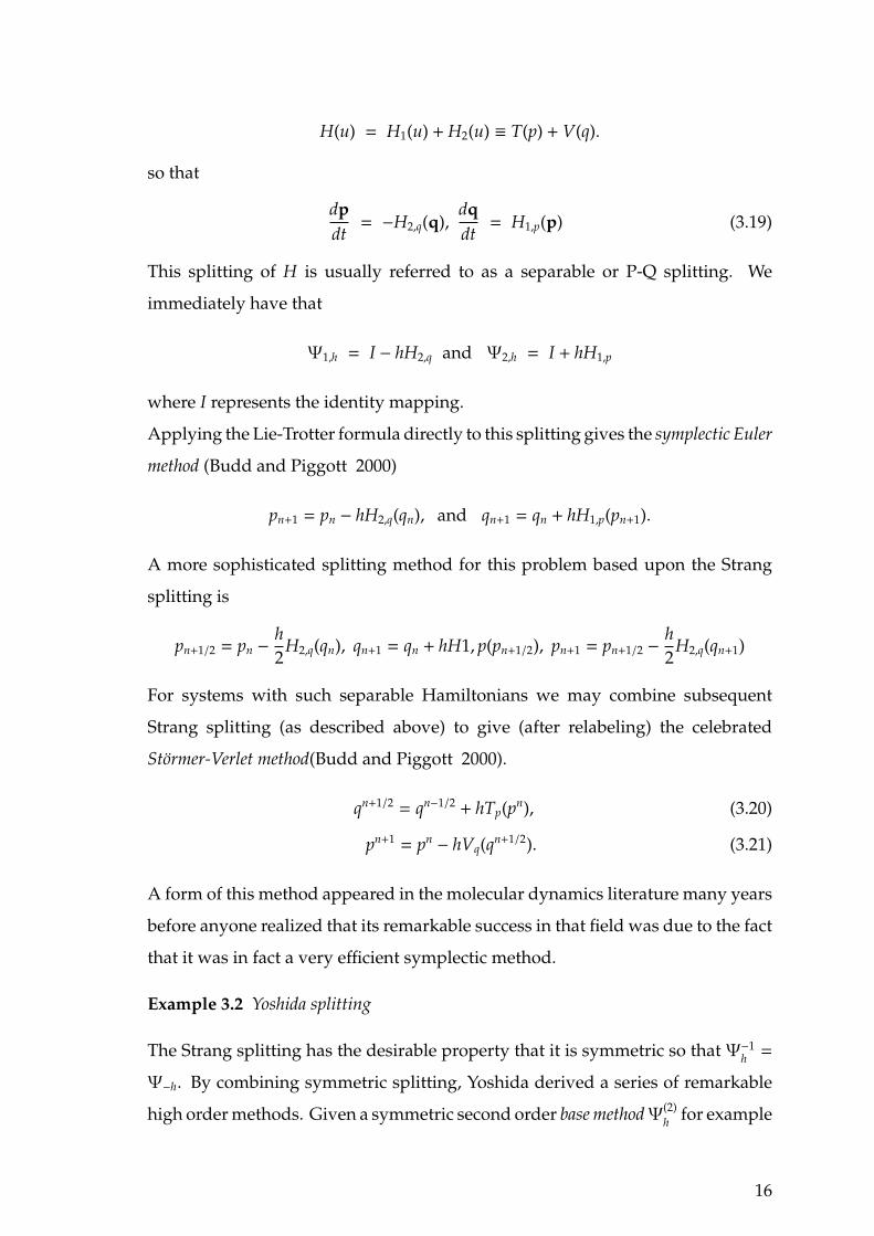
H(u) = H1(u) + H2(u) ≡ T(p) + V(q).
so that
dpdt
= −H2,q(q),dqdt
= H1,p(p) (3.19)
This splitting of H is usually referred to as a separable or P-Q splitting. We
immediately have that
Ψ1,h = I − hH2,q and Ψ2,h = I + hH1,p
where I represents the identity mapping.
Applying the Lie-Trotter formula directly to this splitting gives the symplectic Euler
method (Budd and Piggott 2000)
pn+1 = pn − hH2,q(qn), and qn+1 = qn + hH1,p(pn+1).
A more sophisticated splitting method for this problem based upon the Strang
splitting is
pn+1/2 = pn − h2
H2,q(qn), qn+1 = qn + hH1, p(pn+1/2), pn+1 = pn+1/2 − h2
H2,q(qn+1)
For systems with such separable Hamiltonians we may combine subsequent
Strang splitting (as described above) to give (after relabeling) the celebrated
Stormer-Verlet method(Budd and Piggott 2000).
qn+1/2 = qn−1/2 + hTp(pn), (3.20)
pn+1 = pn − hVq(qn+1/2). (3.21)
A form of this method appeared in the molecular dynamics literature many years
before anyone realized that its remarkable success in that field was due to the fact
that it was in fact a very efficient symplectic method.
Example 3.2 Yoshida splitting
The Strang splitting has the desirable property that it is symmetric so that Ψ−1h =
Ψ−h. By combining symmetric splitting, Yoshida derived a series of remarkable
high order methods. Given a symmetric second order base method Ψ(2)h for example
16

in Yoshida considers the case where the base method is given by the Strang
splitting (Budd and Piggott 2000). Yoshida then constructs the method
Ψ(4)h = Ψ(2)
x1h ◦Ψ(2)x0h ◦Ψ(2)
x1h.
He proved that Ψ(4)h is indeed a fourth-order symmetric method if the weights are
chosen as
x0 = − 21/3
2 − 21/3 , x1 =1
2 − 21/3 .
If the problem being considered is Hamiltonian and the second-order method is
symplectic then our newly constructed fourth-order method will also be sym-
plectic. This procedure can be extended and generalized as follows. Given a
symmetric integrator Ψ(2n)h of order 2n, for example when n = 1 we are sim-
ply restating the above construction and when n = 2 we may take the method
constructed above. The method given by the composition
Ψ(2n+2)h = Ψ(2n+2)
x1h ◦Ψ(2n)x0h ◦Ψ(2n)
x1h
will be a symmetric method of order 2n + 2 if the weights are chosen as
x0 = − 21/(2n+1)
2 − 21/(2n+1), x1 =
12 − 21/(2n+1)
.
3.9. The Adjoint of a Method
The flow ϕt of an autonomous differential equation
y = f (y) y(t0) = y0 (3.22)
satisfies ϕ−1−t = ϕt.
yn+1 = ϕh(yn)⇒
ynϕh−→yn+1
ynϕ−1h←−−
yn+1
yn+1ϕ−h−−→yn
(3.23)
Definition 3.2 The adjoint method Φ∗h of a method Φh is the inverse map of the original
method with reversed time step -h, i.e.,
Φ∗h := Φ−1−h (3.24)
17

In other words, y1 = Φ∗h(y0) is implicitly defined by Φ−h(y1) = y0. A method for
which Φ∗h := Φh is called symmetric (J.M. Sanz Serna 1994).
Lemma 3.1 Implicit Euler Method is the adjoint of explicit Euler Method.
Proof:
Implicit Euler Method→ yn+1 = yn + h f (yn+1)
Explicit Euler Method→ yn+1 = yn + h f (yn+1)
yn+1 = ϕh(yn)
yn+1 = ϕ−h(yn)
yn = ϕ−1−h(yn+1) = ϕ∗h
exchanging h by -h and (n+1) by (n)
yn = yn+1 − h f (yn)⇒ yn+1 = yn + h f (yn) (3.25)
then we proved that the adjoint of explicit Euler method is implicit Euler method.
18

CHAPTER 4
CONSERVED QUANTITIES AND GEOMETRIC
INTEGRATION
In this chapter we give both geometric structures of differential equations
and numerical methods that we consider in chapter 3. We consider three geometric
structures, first integrals, symplecticity and reversibility and symmetry. We give
examples of differential equations which have these geometric features. Then we
mention which of the methods introduced in Chapter 3 preserve first integrals
and have symplecticity or reversibility properties. Finally we give the philosophy
of geometric integration.
4.1. Exact Conservation of Invariants
This section is devoted to the conservation of invariants (first integrals).
First we give the definition of first integral or invariant of a differential equation.
Definition 4.1 : A non-constant function I(y) is called a first integral of the system
y = f (y) , if
dIdt
= I′y′ = I′ f = 0 f or all y (4.1)
This implies that every solution y(t) of I′(y) f (y) = 0 satisfies I(y(t)) = I(y0) =
Const.
For example:
u′ = u(v − 2) (4.2)
v′ = v(1 − u) (4.3)
is the Lotka-Volterra system of equations. Equations (4.2) and (4.3) constitute
an autonomous system of differential equations. This system of equations has
I(u; v) = ln u − u + 2 ln v − v as f irst integral. (Hairer, et al. 2001)
Since
dIdt
=1u.u′ − u′ +
2v.v′ − v′
19

substituting the (4.2) and (4.3) in above derivation
dIdt
=1u.u(v − 2) − u(v − 2) +
2v.v(1 − u) − v(1 − u)
= v − 2 − uv + 2u + 2 − 2u − v + uv = 0.
Lemma 4.1 :Conservation of the Total Energy
Every Hamiltonian system is of the form
p = −Hq(p, q), q = Hp(p, q) (4.4)
the Hamiltonian function H(p, q) is a first integral for every Hamiltonian system
is of the above form.
Proof : This follows at once from
H′(p, q) = ( ∂H∂p ,
∂H∂q ) and
dHdt
=∂H∂p
(−∂H∂q
) +∂H∂q
(∂H∂p
) = 0
Example 4.1 : Conservation of the Total and Angular Momentum of N-Body
systems.
We consider a system of N particles interacting pairwise with potential forces
which depend on the distance between the particles. This is formulated as a
Hamiltonian system with total energy
H(p, q) =12
N∑
i=1
1mi
pTi pi +
N∑
i=1
N∑
i, j=1
Vi j(‖ qi − q j ‖) (4.5)
Here pi, qi ∈ R3 represent the position and momentum of the ith particle of
mass mi and Vi j (i > j) is the interaction potential between the ith and jth particle.
The equations of motion read
qi =1
mipi, pi =
N∑
j=1
vi j(qi − q j) (4.6)
where, for i > j we have vi j = v ji = V′i j(ri j)/ri j with ri j =‖ qi−q j ‖, and vii is arbitrary,
say vii = 0. The conservation of the total linear momentum P =∑N
i=1 pi and the
angular momentum L =∑N
i=1 qi × pi is the consequences of symmetry relation
20
vi j = v ji
ddt
N∑
i=1
pi =
N∑
i=1
N∑
j=1
vi j(qi − q j) = 0 (4.7)
ddt
N∑
i=1
qi × pi =
N∑
i=1
1mi
pi × pi +
N∑
i=1
N∑
j=1
qi × vi j(qi − q j) = 0 (4.8)
Theorem 4.1 (Conservation of Linear First Integrals) : All explicit and implicit
Runge-Kutta methods as well as multi-step methods conserve linear first integrals. Par-
titioned Runge-Kutta methods conserve linear first integrals only if bi = bi for all i, or if
the first integral only depends on p alone or only on q alone.
Proof : Let I(y) = bT y with constant vector b, so that bT f (y) = 0 f or all y. In the
case of Runge-Kutta methods we thus have bTki = 0, and consequently bT y1 =
bT y0 + hbT(∑s
i=1 biki) = bT y0. The statement for partitioned method is proved
similarly.
4.1.1. Quadratic Invariants
Quadratic invariants appear often in applications. Conservation of the an-
gular momentum is an example of quadratic invariants. We consider differential
equation y′ = f (y) and quadratic function
Q(y) = yTCy
where C is a symmetric square matrix. It is an invariant of y′ = f (y) if yTC f (y) =
0 f or all y (Hairer, et al. 2001).
Since yTC f (y) = 0
Q′(y) = (y′)TCy + yTCy′ = ( f (y))TCy + yTC f (y)
= (yTC f (y))T + yTC f (y) = 0
Theorem 4.2 If the coefficients of a Runge-Kutta method satisfy
biai j + b ja ji = bib j (4.9)
then it conserves quadratic invariants.
21
Proof: See (Hairer, et al. 2001).
We next consider partitioned Runge-Kutta methods for systems y = f (y, z) z =
g(y, z). Usually such methods cannot conserve general quadratic invariants. We
therefore concentrate on quadratic invariants of the form
Q(y, z) = yTDz
where D is a matrix of appropriate dimensions. Observe that the angular mo-
mentum is of this form.
Theorem 4.3 Sormer-Verlet scheme conserves all quadratic invariants of the form
Q(y, z) = yTDz.
Proof: See (Hairer, et al. 2001).
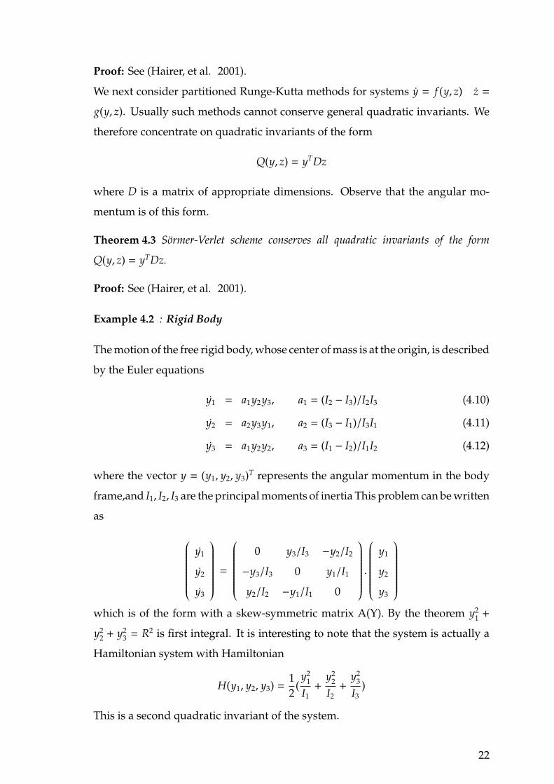
Example 4.2 : Rigid Body
The motion of the free rigid body, whose center of mass is at the origin, is described
by the Euler equations
y1 = a1y2y3, a1 = (I2 − I3)/I2I3 (4.10)
y2 = a2y3y1, a2 = (I3 − I1)/I3I1 (4.11)
y3 = a1y2y2, a3 = (I1 − I2)/I1I2 (4.12)
where the vector y = (y1, y2, y3)T represents the angular momentum in the body
frame,and I1, I2, I3 are the principal moments of inertia This problem can be written
as
y1
y2
y3
=
0 y3/I3 −y2/I2
−y3/I3 0 y1/I1
y2/I2 −y1/I1 0
.
y1
y2
y3
which is of the form with a skew-symmetric matrix A(Y). By the theorem y21 +
y22 + y2
3 = R2 is first integral. It is interesting to note that the system is actually a
Hamiltonian system with Hamiltonian
H(y1, y2, y3) =12
(y2
1
I1+
y22
I2+
y23
I3)
This is a second quadratic invariant of the system.
22

We present in Figure(4.1) the sphere with some of the solutions of corre-
sponding to I1 = 2, I2 = 1 and I3 = 2/3. In the left picture we have included the
numerical solution (30 steps) obtained by the implicit midpoint rule with step
size h = 0,3 and initial value y0 = (cos(1.1); 0; sin(1.1))T. It stays exactly on a so-
lution curve. This follows from the fact that the implicit midpoint rule preserves
quadratic invariants exactly. For the explicit Euler method (right picture, 320
steps with h = 0.05 and the same initial value as above) we see that the numerical
solution shows the wrong qualitative behaviour (it should lie on a closed curve).
The numerical solution even drifts away from the manifold (Hairer, et al. 2001)
Figure 4.1. Solution of the Euler equations (4.10),(4.11),(4.12) for the rigid body.
4.2. Symplectic Transformations
In this section we discuss the symplecticity property. The basic objects
to be studied are two-dimensional parallelograms lying in R2d. We suppose the
parallelogram to be spanned by two vectors
ξ =
ξp
ξq
, η =
ηp
ηq
in the (p, q) space (ξp, ξq, ηp, ηq are in Rd) as
P = {tξ + sη|0 ≤ t ≤ 1, 0 ≤ s ≤ 1}.
23

In the case d=1 we consider the oriented area
Area(P) = det
ξp ηp
ξq ηq
= ξpηq − ξqηp
In higher dimensions, we replace this by the sum of the oriented areas of the
projections of P onto the coordinate planes (pi, qi), i.e., by
ω(ξ, η) :=d∑
i=1
det
ξp
i ηpi
ξqi ηq
i
=
d∑
i=1
(ξpi η
qi − ξ
qi η
pi ).
This defines a bilinear map acting on vectors ofR2d, which will play a central role
for Hamiltonian system. In matrix notation, this map has the form
ω(ξ, η) = ξT Jη with J =
0 I
−I 0
where I is the identity matrix of dimension d (Hairer, et al. 2001).
Definition 4.2 A linear mapping A : R2d → R2d is called symplectic if
AT JA = J
or, equivalently, if ω(Aξ,Aη) = ω(ξ, η) for all ξ, η ∈ R2d.
We can find it
ω(Aξ,Aη) = (Aξ)T J(Aη) = ξT AT JA︸︷︷︸ η (since AT JA = J)
= ξT Jη = ω(ξ, η)
Definition 4.3 For nonlinear mapping, the differentiable functions can be locally ap-
proximated by linear functions. A differentiable map g : U→ R2d (where U ⊂ R2d is an
open set) is called symplectic if the Jacobian matrix g′(p, q) is everywhere symplectic, i.e.,
if
g′(p, q)T Jg′(p, q) = J or ω(g′(p, q)ξ, g′(p, q)η) = ω(ξ, η).
Lemma 4.2 If ψ and ϕ are symplectic maps then ψ ◦ ϕ is symplectic.
Proof: Since ψ is symplectic
(ψ′)T Jψ′ = J, similarly (ϕ′)T Jϕ′ = J[(ψoϕ)′
]TJ(ψoϕ)′ = (ψ′oϕ′)T J(ψ′oϕ′) = (ϕ′)To(ψ′)T Jψ′oϕ′ = J
24
Theorem 4.4 (Poincare 1899). Let H(p, q) be a twice continuously differentiable function
on U ⊂ R2d. Then, for each fixed t, the flow ϕt is a symplectic transformation wherever
it is defined.
Proof: Let ϕt be flow of the Hamiltonian system. ϕ′t is a Jacobian matrix of the
flow, then ϕ′t satisfies the variational equation i.e.
ddtϕ′t = J−1H′′ϕ′t where H′′ =
Hpp Hpq
Hqp Hqq
is symmetric.
Henceddt
(ϕ′Tt Jϕ′t) = [J−1H′′ϕ′t]T Jϕ′t + ϕ′Tt JJ−1
︸︷︷︸ H′′ϕ′t
since JJ−1 = Iddt
(ϕ′Tt Jϕ′t) = ϕ′Tt H′′T (J−1)T J︸ ︷︷ ︸ϕ′t + ϕ′Tt H′′ϕ′t
now, we will use (H′′)T = H′′ and (J−1)T J = −I, let us prove it;
JT = −J
[(J−1)T J]T = JT · J−1 = −J · J−1 = −I
then we finally find (J−1)T J = −I. We put (J−1)T J = −I in the last equation;
ddt
(ϕ′Tt Jϕ′t) = −ϕ′Tt H′′ϕ′t + ϕ′Tt H′′ϕ′t = 0
Since ddt(ϕ
′Tt Jϕ′t) = 0 then ϕ′Tt Jϕ′t = C. When t = 0, we have ϕ′t(t0) = I⇒ C = J
Theorem 4.5 Let f : U → R2d be continuously differentiable. Then, y = f (y) is locally
Hamiltonian if and only if its flow ϕt(y) is symplectic for all y ∈ U and for all sufficiently
small t.
Proof: Assume that the flow ϕt is symplectic, and we have to prove the local
existence of a function H(y) such that f (y) = J−1∇H(y). Using the fact that ∂ϕt
∂y0is a
solution of the variational equation Ψ = f ′(ϕt(y0))Ψ, we obtain
ddt
((∂ϕt
∂y0
)TJ(∂ϕt
∂y0
))=
(∂ϕt
∂y0
)(f ′(ϕt(y0))T J + J f ′(ϕt(y0)
)(∂ϕt
∂y0
)= 0.
Putting t = 0, it follows from J = −JT that J f ′(y0) is a symmetric matrix for all y0.
25

Theorem 4.6 Let ψ : U → V be a change of coordinates such that ψ and ψ−1 are
continuously differentiable functions. If ψ is symplectic, the Hamiltonian system y =
J−1∇H(y) becomes in the new variables z = ψ(y)
z = J−1∇K(z) with K(z) = H(y).
Conversely, if ψ transforms every Hamiltonian system to another Hamiltonian system,
then ψ is symplectic.
Proof: Since z = ψ′(y)y and ψ′(y)T∇K(z) = ∇H(y), the Hamiltonian system y =
J−1∇H(y) becomes
z = ψ′(y)J−1ψ′(y)T∇K(z)
in the new variables. It is equivalent to z = J−1∇K(z) with K(z) = H(y) if
ψ′(y)J−1ψ′(y)T = J−1.
Multiplying this relation from the right byψ′(y)−T and from the left byψ′(y)−1 and
then taking its inverse yields J = ψ′(y)T Jψ′(y), which shows that the last equation
is equivalent to the symplecticity of ψ.
4.3. Examples of Symplectic Integrators
Definition 4.4 A numerical one-step method is called symplectic if the one-step map
y1 = Φh(y0) is symplectic whenever it is applied to a smooth Hamiltonian system.If the
method is symplectic:
Φ′h(y)T J Φ′h(y) = J (4.13)
where J =
0 I
−I 0
Theorem 4.7 The implicit midpoint rule is symplectic.
Proof : The second order implicit midpoint rule is:
Un+1 = Un + h f(Un + Un+1
2
)(4.14)
Consider the Hamiltonian problem
y = J−1∇H(y) (4.15)
26
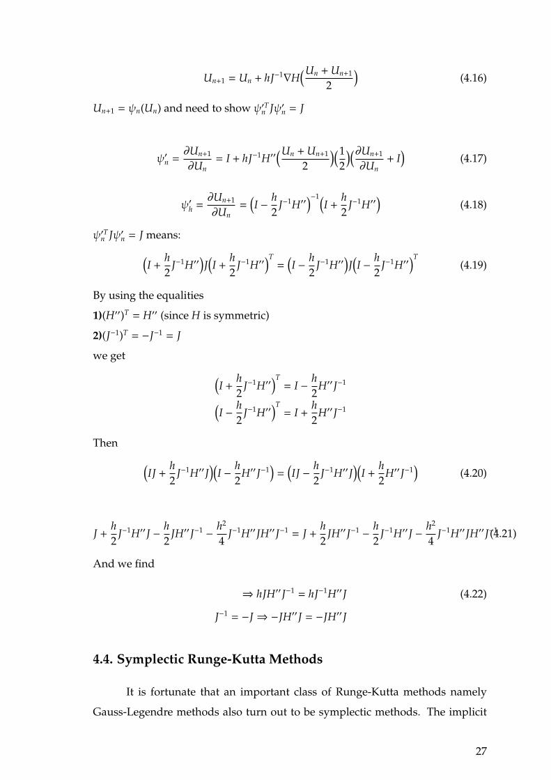
Un+1 = Un + hJ−1∇H(Un + Un+1
2
)(4.16)
Un+1 = ψn(Un) and need to show ψ′Tn Jψ′n = J
ψ′n =∂Un+1
∂Un= I + hJ−1H′′
(Un + Un+1
2
)(12
)(∂Un+1
∂Un+ I
)(4.17)
ψ′h =∂Un+1
∂Un=
(I − h
2J−1H′′
)−1(I +
h2
J−1H′′)
(4.18)
ψ′Tn Jψ′n = J means:
(I +
h2
J−1H′′)J(I +
h2
J−1H′′)T
=(I − h
2J−1H′′
)J(I − h
2J−1H′′
)T(4.19)
By using the equalities
1)(H′′)T = H′′ (since H is symmetric)
2)(J−1)T = −J−1 = J
we get
(I +
h2
J−1H′′)T
= I − h2
H′′J−1
(I − h
2J−1H′′
)T= I +
h2
H′′J−1
Then
(IJ +
h2
J−1H′′J)(
I − h2
H′′J−1)
=(IJ − h
2J−1H′′J
)(I +
h2
H′′J−1)
(4.20)
J +h2
J−1H′′J − h2
JH′′J−1 − h2
4J−1H′′JH′′J−1 = J +
h2
JH′′J−1 − h2
J−1H′′J − h2
4J−1H′′JH′′J−1(4.21)
And we find
⇒ hJH′′J−1 = hJ−1H′′J (4.22)
J−1 = −J⇒ −JH′′J = −JH′′J
4.4. Symplectic Runge-Kutta Methods
It is fortunate that an important class of Runge-Kutta methods namely
Gauss-Legendre methods also turn out to be symplectic methods. The implicit
27
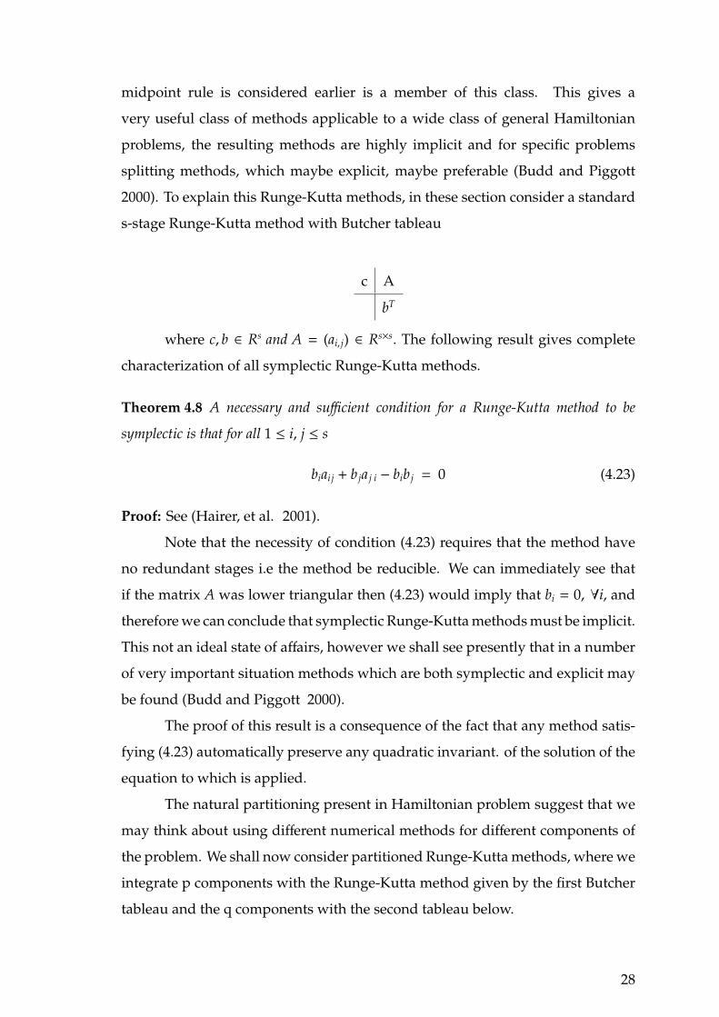
midpoint rule is considered earlier is a member of this class. This gives a
very useful class of methods applicable to a wide class of general Hamiltonian
problems, the resulting methods are highly implicit and for specific problems
splitting methods, which maybe explicit, maybe preferable (Budd and Piggott
2000). To explain this Runge-Kutta methods, in these section consider a standard
s-stage Runge-Kutta method with Butcher tableau
c A
bT
where c, b ∈ Rs and A = (ai, j) ∈ Rs×s. The following result gives complete
characterization of all symplectic Runge-Kutta methods.
Theorem 4.8 A necessary and sufficient condition for a Runge-Kutta method to be
symplectic is that for all 1 ≤ i, j ≤ s
biai j + b ja j i − bib j = 0 (4.23)
Proof: See (Hairer, et al. 2001).
Note that the necessity of condition (4.23) requires that the method have
no redundant stages i.e the method be reducible. We can immediately see that
if the matrix A was lower triangular then (4.23) would imply that bi = 0, ∀i, and
therefore we can conclude that symplectic Runge-Kutta methods must be implicit.
This not an ideal state of affairs, however we shall see presently that in a number
of very important situation methods which are both symplectic and explicit may
be found (Budd and Piggott 2000).
The proof of this result is a consequence of the fact that any method satis-
fying (4.23) automatically preserve any quadratic invariant. of the solution of the
equation to which is applied.
The natural partitioning present in Hamiltonian problem suggest that we
may think about using different numerical methods for different components of
the problem. We shall now consider partitioned Runge-Kutta methods, where we
integrate p components with the Runge-Kutta method given by the first Butcher
tableau and the q components with the second tableau below.
28

c A
bT
c A
bT
As we have done for symplectic Runge-Kutta methods we may now classify
partitioned Runge-Kutta methods with the following result.
For special case of problems where the Hamiltonian take the separable form
H(p, q) = T(p) + V(q) only the second part of (4.23) is required for symplecticity.
An example of such a method by Ruth’s third order method it has been
tableau
7/24 0 0
c 7/24 3/4 0
7/24 3/4 -1/24
7/24 3/24 -1/24
0 0 0
c 2/3 0 0
2/3 -2/3 0
2/3 -2/3 1
Theorem 4.9 If the coefficients of a partitioned Runge-Kutta method satisfy
biai j + b ja ji = bib j f or i, j = 1, ...., s, (4.24)
bi = bi f or i = 1, ...., s, (4.25)
then it is symplectic.
Theorem 4.10 A symplectic Runge-Kutta method leaves all quadratic first integrals
of a hamiltonian system invariant, i.e. if yn = (pn, qn) and G = Gt ∈ M2d(R),then
ytn+1Gyn+1 = yt
nGyn for all n.
In particular, if a linear autonomous system is integrated with a symplectic
Runge-Kutta method, than the energy will be conserved exactly (up to truncation
errors, of course).
4.5. Examples of Applications of Symplectic Integrators
In these section we look the application of symplectic integrators to the
harmonic oscillator as a Hamiltonian system.
The Harmonic Oscillator
This well studied problem has a separable Hamiltonian of the form
H(p, q) =p2
2+
q2
2, (4.26)
29

and has solutions which are circles in the (p,q) phase space. The associated
differential equations are
dqdt
= p,dpdt
= −q. (4.27)
Consider now the closed curve (circle)
Γ ≡ p2 + q2 = C2,
the action of the solution operator of the differential equation is to map this curve
into itself(conserving the area πC2 of the enclosed region). The standard forward
Euler method applied to this system gives the scheme
pn+1 = pn − hqn, qn+1 = qn + hpn, (4.28)
so that Ψh is the operator given by
Ψhv =
1 −h
h 1
v, with det(Ψh) = 1 + h2.
It is easy to see that in this case,Γ evolves through the action of the discrete map
Ψh to the new circle given by
p2n+1 + q2
n+1 = C2(1 + h2) (4.29)
and the area enclosed within the discrete evolution of Γ has increased by a factor
of 1 + h2. Periodic orbits are not preserved by the forward Euler method – indeed
all such discrete orbits spiral to infinity. Similarly, a discretisation using the
backward Euler method leads to trajectories that spiral towards the origin (Budd
and Piggott 2000).
Consider now the symplectic Euler method applied to this example. This gives rise
to the discrete map
pn+1 = pn − hqn, qn+1 = qn + h(pn − hqn) = (1 − h2)qn + hpn (4.30)
The discrete evolutionary is then simply matrix
Ψh
p
q
=
1 −h
h 1 − h2
p
q
30

which can easily be checked to be symplectic. For example det(Ψh)=1. The circle
Γ is now mapped to the ellipse
(1 − h2 + h4)p2n+1 − 2h3pn+1qn+1 + (1 + h2)q2
n+1 = C2 (4.31)
which has the same enclosed area. The symplectic Euler map is not symmetric in
time so that
ψ−1h , ψ−h.
Observe that the symmetry of the circle has been destroyed through the applica-
tion of this mapping.
It is also easy to see that if
A =
1 −h
2
−h2 1
then
ΨTh AΨh = A.
Next consider the Stormer-Verlet method. This gives the discrete map
pn+1/2 = pn − hqn/2, qn+1 = qn + h(pn − hqn/2), (4.32)
pn+1 = pn+1/2 − h2
(qn + h(pn − h2
qn)). (4.33)
The discrete evolutionary operator ψh is now the symplectic matrix
Ψhv =
1 − h2/2 −h + h3/4
h 1 − h2/2
v.
The curve Γ is to order h2 mapped to a circle of the same radius. The Stormer-
Verlet method preserves the symmetry of the circle to this order, and indeed is
also symmetric in time so that ψ−1 = ψ−h.
Finally we consider the implicit midpoint rule. For this we have
C
pn+1
qn+1
= CT
pn
qn
,
where
C =
1 h
2
−h2 1
.
31

Observe that CCT = (1 + h2/4)I. The evolution operator is then simply
Ψh = C−1CT.
Observe further that if Un = (pn, qn)T then
(1 + h2/4)UTn+1Un+1 = UT
n+1CTCUn+1 = UTnCCTUn = (1 + h2/4)UT
nUn.
Hence the quadratic invariant UTnUn is exactly preserved by this method. This
feature is shared by all symplectic Runge-Kutta methods.
4.6. Symmetric Integration and Reversibility
Symmetric methods of this chapter and symplectic methods of preceding
chapter play a center role in the geometric integration of differential equations.
We discuss reversible differential equations and reversible maps, and we explain
how symmetric integrators are related to them. We study symmetric Runge-Kutta
and composition methods.
4.6.1. Reversible Differential Equations and Maps
Conservative mechanical systems have the property that inverting the
initial direction of the velocity vector and keeping the initial position does not
change the solution trajectory, it only inverts the direction of motion (Hairer, et
al. 2001). Such systems are ’reversible’. We extend this notion to more general
situations.
Figure 4.2. Reversible vector field (left picture) and reversible map (right picture)
32

Definition 4.5 Letρ be an invertible linear transformation in the phase space of y = f (y).
This differential and vector field f (y) called ρ − reversible if
ρ f (y) = − f (ρy) for all y. (4.34)
This property is illustrated in the left picture of Figure(4.3). For ρ − reversible
differential equations the exact flow ϕt(y) satisfies
ρ ◦ ϕt = ϕ−t ◦ ρ = ϕ−1t ◦ ρ (4.35)
Lemma 4.3 Show the equality is true.
ρ ◦ ϕt = ϕ−t ◦ ρ = ϕ−1t ◦ ρ (4.36)
Proof: The right identity is a consequence of the group property
ϕt ◦ ϕs = ϕt+s, ϕt ◦ ϕ−t = I, ϕ−t = ϕ−1t ,
and the left identity follows from y = f (y), ϕt is exact flow then ddt (ϕt) = f (ϕt) and
ρ(ϕt) is also solution of equation
ddt
(ρ ◦ ϕt)(y) = ρ f (ϕt(y)) = − f ((ρ ◦ ϕt)(y))
ddt
(ϕ−t ◦ ρ)(y) = − f ((ϕ−t ◦ ρ)(y))
Definition 4.6 A map Φ(y) is called ρ − reversible if
ρ ◦Φ = Φ−1 ◦ ρ (4.37)
Example 4.3 : An important example is the partitioned system
u = f (u, v), v = g(u, v) (4.38)
where f (u,−v) = − f (u, v) and g(u,−v) = g(u, v). Here, the transformation ρ is
given by ρ(u, v) = (u,−v). If we call a vector field or a map reversible (without
specifying the transformationρ), we mean that it isρ−reversible with this particular
ρ.
−ρ f (y) = f (ρ(y))
33

f (u,−v) = − f (u, v)
g(u,−v) = g(u, v)
ρ(u, v) = (u,−v) where (u, v) = Y
f (ρ(Y)) = f (u,−v) = − f (u, v) (∗)
f (Y) = f (u, v) = − f (u,−v)
ρ( f (Y)) = f (u, v) (∗∗)
from (∗) and (∗∗)f (ρ(Y)) = −ρ( f (Y))
u = g(u) is always reversible system. u = v = f (u, v), v = g(u)
f (u,−v) = −v = − f (u, v)
Definition 4.7 A numerical one-step method Φh is called symmetric or time-reversible,
if it satisfies
Φh ◦Φ−h = id or equaivalently Φh = Φ−1−h
With the definition of adjoint method (Φ∗h = Φ−1−h), the condition for symmetry reads
Φh = Φ∗h. A method y1 = Φh(y0) is symmetric if exchanging y0 ↔ y1 and h ↔ −h
leaves the method unaltered. Implicit midpoint rule and the Stormer-Verlet scheme both
of which are symmetric.
Theorem 4.11 If a numerical method, applied to a ρ − reversible differential equation
satisfies
ρ ◦Φh = Φ−h ◦ ρ, (4.39)
then the numerical flow Φh is a ρ− reversible map if and only if Φh is a symmetric method.
Proof: As a consequence of (4.30) the numerical flow Φh is ρ − reversible if and
only if Φ−h ◦ ρ = Φ−1h ◦ ρ. Since ρ is an invertible transformation, this is equivalent
to the symmetry of the method Φh.
34

Example 4.4 : Explicit method Φh(y0) = y0 + h f (y0)
ρ ◦Φh(y0) = ρ(y0 + h f (y0)) = ρy0 + hρ f (y0) = ρy0 − h f (ρ(y0)) = Φ−h(ρ(y0))
Hence
ρ ◦Φh = Φ−h ◦ ρ.
Similarly, it is also true that a symmetric method is ρ − reversible if and only
if the ρ-compatibility condition (4.37) holds. Compared to the system of the
method, condition (4.37) is much less restrictive. It is automatically satisfied by
most numerical methods. Let us briefly discuss the validity of (4.37) for different
classes of methods.
• Runge-Kutta Methods(explicit or implicit) satisfy (4.37) without any restric-
tion other than (4.36) on the vector field. Let us illustrate the proof with the
explicit Euler method Φh(y0) = y0 + h f (y0):
(ρ ◦Φh)(y0) = ρy0 + hρ f (y0) = ρy0 − h f (ρy0) = Φ−h(ρy0)
(Hairer, et al. 2001)
• Partitioned Runge-Kutta Methods applied to a partitioned system satisfy the
condition (4.37) if ρ(u, v) = (ρ1(u), ρ2(v)) with invertible ρ1 and ρ2. The
proof is the same as for Runge-Kutta methods. Notice that the mapping
ρ(u, v) = (u,−v) of example (4.3) is of this special form (Hairer, et al. 2001).
• Composition methods. If two methods Φh and Ψh satisfy (4.37), then so does
the adjoint Φ∗h and the composition Φh ◦Ψh. Consequently, the composition
methods, which compose a basic method Φh and its adjoint with different
step sizes, have the property (4.37) provided the basic method Φh has it
(Hairer, et al. 2001).
• Splitting methods are based on a splitting y = f [1](y)+ f [2](y) of the differential
equation. If both vector fields, f [1](y) and f [2](y), satisfy (1), then their exact
flows ϕ[1]h and ϕ[2]
h satisfy (4.36). In this situation, the splitting method has
the property (4.37) (Hairer, et al. 2001).
35

4.7. Examples of Symmetric Methods
Now we introduce some symmetric methods in this section.
Lemma 4.4 Midpoint rule is a symmetric method.
Proof: The midpoint rule is
yn+1 = yn + h f( yn+1 + yn
2
)
exchanging h by -h and (n+1) by (n)
yn = yn+1 − h f( yn+1 + yn
2
)
yn+1 = yn + h f( yn+1 + yn
2
)
then we proved that midpoint rule is symmetric.
Lemma 4.5 Trapezoidal rule is symmetric.
Proof: Trapezoidal rule is
yn+1 = yn +h2
[f (yn) + f (yn+1)
]
exchanging h by -h and (n+1) by (n)
yn = yn+1 − h2
[f (yn+1) + f (yn)
]
yn+1 = yn +h2
[f (yn) + f (yn+1)
]
then we proved that trapezoidal rule is symmetric.
4.8. Geometric Structures in Hamiltonian Systems
We can write the Hamiltonian systems of the form:
p = − 5q H(p, q), q = 5pH(p, q) (4.40)
where H : Rd×Rd → R, and the dimension d is the number of degrees of freedom.
In applications the Hamiltonian is often given in the form:
H(p, q) =12
pTM(q)−1p + U(q) (4.41)
36

with a positive definite symmetric mass matrix M(q) and a potential U(q).In this
situation, the function H(p, q) represents the total energy of the system. Such
problems arise in mechanics, astrophysics,molecular dynamics, and many other
sciences (Hairer 2005).
Due to their special structure, Hamiltonian systems have several interesting
properties (in the following we denote the flow of the system, mapping an initial
value y = (p, q) onto the solution at time t, by ϕt(y)):
(P1) the group property ϕt oϕs = ϕt+s is satisfied by every differential
equation; in particular, one has
ϕt oϕ−t = ϕ0 = identity (4.42)
(P2) the Hamiltonian H(p, q) is constant along solutions of (5.32) which
means that the total energy is conserved quantity,
(P3) the flow ϕt of (4.40) is a symplectic transformation, i.e.
ϕ′t(y)T Jϕ
′t(y) = J f or t ≥ 0, J =
0 I
−I o
(4.43)
Due to det ϕ′t(y) = 1, this implies the flow is volume preserving,
µ(ϕt(A)) = µ(A) t ≥ 0
and for the system with one degree of freedom symplecticity turns out to be
equivalent with area-preservation of the flow ϕt,
(P4) if H(−p, q) = H(p, q), the flow ϕt is ρ-reversible with respect to the
reflection ρ(p, q) = (−p, q), i.e. it satisfies
(ρ o ϕt)(y) = (ϕ−1t o ρ)(y) f or all t and all y.
It is natural to look for numerical methods that satisfy one or several of
these properties.
4.9. Geometric Integration
As we mentioned in chapter 3 that a numerical method for solving ordinary
differential equations is a mapping Φh defined on the phase space that approxi-
mates the time-h flow ϕh; if Φh(y) = ϕh(y)+O(hr+1). The numerical approximation
37
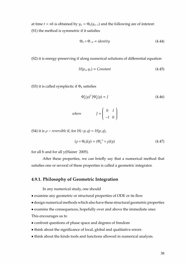
at time t = nh is obtained by yn = Φh(yn−1) and the following are of interest:
(S1) the method is symmetric if it satisfies
Φh ◦Φ−h = identity (4.44)
(S2) it is energy-preserving if along numerical solutions of differential equation
H(pn, qn) = Constant (4.45)
(S3) it is called symplectic if Φh satisfies
Φ′h(y)T JΦ′h(y) = J (4.46)
where J =
0 I
−I 0
(S4) it is ρ − reversible if, for H(−p, q) = H(p, q),
(ρ ◦Φh)(y) = (Φ−1h ◦ ρ)(y) (4.47)
for all h and for all y(Hairer 2005).
After these properties, we can briefly say that a numerical method that
satisfies one or several of these properties is called a geometric integrator.
4.9.1. Philosophy of Geometric Integration
In any numerical study, one should
• examine any geometric or structural properties of ODE or its flow
•design numerical methods which also have these structural geometric properties
• examine the consequences, hopefully over and above the immediate ones
This encourages us to
• confront questions of phase space and degrees of freedom
• think about the significance of local, global and qualitative errors
• think about the kinds tools and functions allowed in numerical analysis.
38

For example, multi-step methods do not define a map on phase space,
because more than one initial condition required. They can have geometric prop-
erties, but in a different phase space, which can alter the effects of the properties.
This puts geometric integration firmly into the single step. If a system is defined
on a sphere, one should stay on that sphere.
The direct consequences of geometric integration are that we are
• studying a dynamical system which is close to the true one, and the right class
• this class may have restricted orbit types, stability, and long-time behavior
In addition, because the structural properties are so natural, some indirect
consequences have been observed. For example,
• symplectic integrators have good energy behaviors
• symplectic integrators can conserve angular momentum and other conserved
quantities
• geometric integrators can have smaller local truncation errors for special prob-
lems and smaller global truncation errors for special problems/initial conditions
• some problems can have errors tending to zero at long times.
In designing our numerical method to preserve some structure we hope to
see improvements in our computations. Geometric structures often make it easier
to estimate errors, and in fact local and global errors may will be smaller for no
extra computational expense. Geometric integration methods designed to capture
specific qualitative properties may also preserve additional properties of the so-
lution for free. For example symplectic methods for Hamiltonian problems have
excellent energy conservation properties and can conserve angular momentum
or other invariants.
In conclusion, geometric integration methods can often ’go where other
methods cannot’ and the motivation for preserving structure include
(i) it may yield methods that are faster, simpler, more stable, and more accurate,
as in methods for structured eigenvalue problems for some types of ODEs;
(ii) it may yield methods that are more robust and yield qualitatively better re-
sults than standard methods, even if the standard numerical errors are no smaller;
(iii) it may suggest new types of calculations previously thought to be impossi-
ble, as in the long-time integration of Hamiltonian systems;
39

(iv) it may be essential to obtain a useful (e.g convergent) method, as in the
discrete differential complexes used in electromagnetism;
(v) the development of general-purpose methods may be nearing completion,
as in Runge-Kutta methods for ODEs (Hairer 2005).
4.10. The Kepler Problem and Its Conserved Quantities
In classical mechanics, Keplers problem is a special case of the two-body
problem, in which the two bodies interact by a central force F that varies in
strength as the inverse square of the distance r between them. The force may be
either attractive or repulsive. The ”problem” to be solved is to find the position
or speed of the two bodies over time given their masses and initial positions and
velocities. Using classical mechanics, the solution can be expressed as a Kepler
orbit.
Consider two particles in R3. One is fixed at the origin, and the other
one moves under the influence of gravitational field of the fixed particle. The
problem, named after Kepler, is to describe the motion of the second particle.
The following non-dimensional Kepler Problem is considered as a test problem
to perform the geometric and non-geometric integration methods. We define the
Kepler Hamiltonian system:
q = p (4.48)
p = −Gq|q|3 (4.49)
where q is position vector, p is momenta and G is the gravitational constant. In
this section we consider the conserved quantities of the Kepler Problem such that
the energy function, angular momentum and Runge-Lenz vector. The equations
of three dimensional Kepler problem have the following first integrals:
1) Hamiltonian Function:
Total energy of the system is the Hamiltonian function
H(q1, q2, q3, p1, p2, p3) =12
(p21 + p2
2 + p23) − G√
q21 + q2
2 + q23
(4.50)
We showed before that the energy is conserved.
2) Angular Momentum:
40

The system has not only the total energy H(p, q) as a first integral, but also the
angular momentum of a point particle with position−→q and momentum−→p is equal
to the vector cross product of the position and momentum vectors
L = −→q × −→p (4.51)
Angular momentum is another conserved quantity for the Kepler problem. The
time derivative of angular momentum is:
dLdt
=dqdt× p + q × dp
dt
= p × p − K|q|3 q × q = 0
3) Runge-Lenz Vector:
Another conserved quantity of the Kepler Problem is Runge-Lenz vector. For
a single particle acted on by an inverse-square central force described by the
equation F(|q|) = −k|q|2 q, the Runge-Lenz vector A is defined mathematically by the
formula:
A = p × L −mkq
where
•m is the mass of the point particle moving under the central force,
• p is its momentum vector,
• L = q × p is its angular momentum vector,
• k is a parameter that describes strength of the central force,
• q is the position vector of the particle,
• q is the corresponding unit vector, i.e, q =q|q| .
The Runge-lenz vector is conserved quantity of the Kepler problem since:
A central force F acting on the particle is F = f (|q|). q|q| = f (|q|).q. For some function
f (|q|) of the radius q. Since dLdt = 0
ddt
(p × L) =dpdt× L = f (|q|).q × (q × p)
where the momentum p = mdqdt .
ddt
(p × L) = f (|q|). q|q| × (q ×m
dqdt
)
41
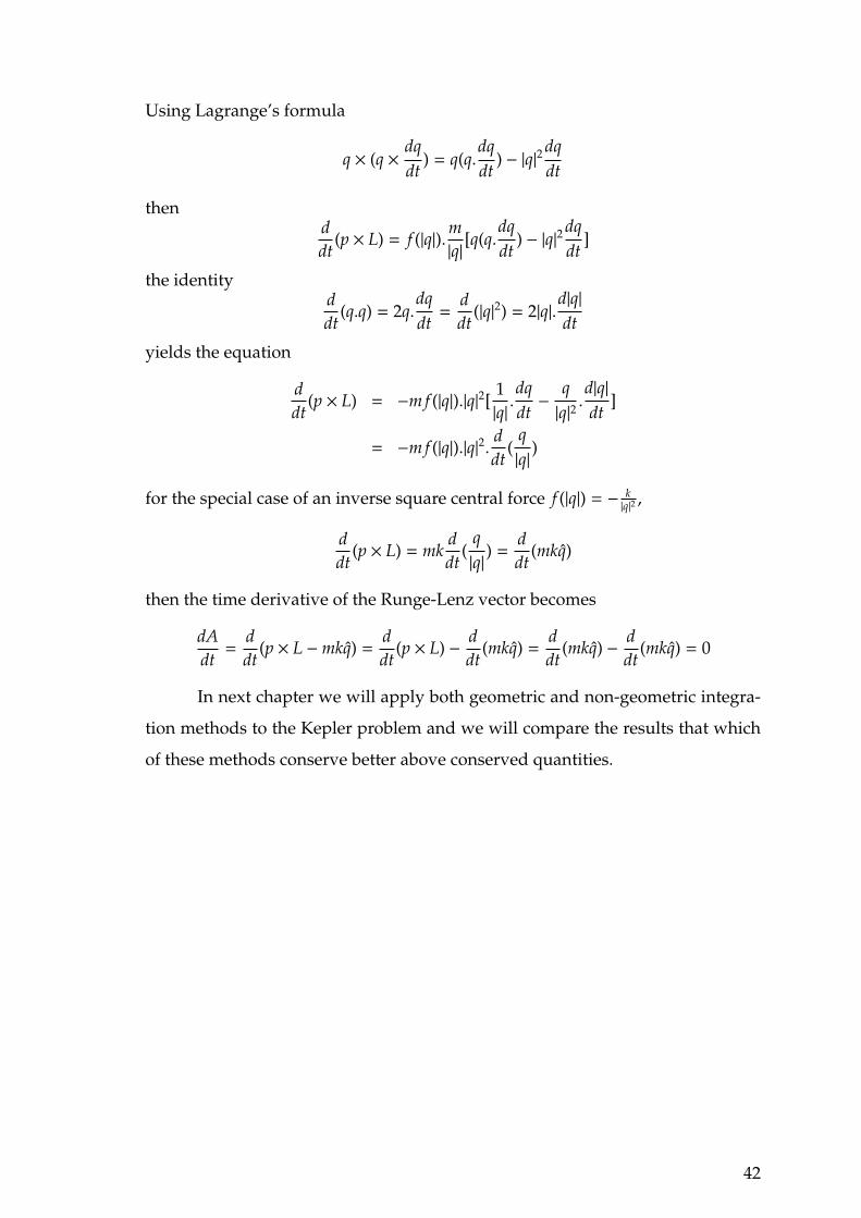
Using Lagrange’s formula
q × (q × dqdt
) = q(q.dqdt
) − |q|2 dqdt
thenddt
(p × L) = f (|q|).m|q|[q(q.dqdt
) − |q|2 dqdt
]
the identityddt
(q.q) = 2q.dqdt
=ddt
(|q|2) = 2|q|.d|q|dt
yields the equation
ddt
(p × L) = −m f (|q|).|q|2[1|q| .
dqdt− q|q|2 .
d|q|dt
]
= −m f (|q|).|q|2. ddt
(q|q| )
for the special case of an inverse square central force f (|q|) = − k|q|2 ,
ddt
(p × L) = mkddt
(q|q|) =
ddt
(mkq)
then the time derivative of the Runge-Lenz vector becomes
dAdt
=ddt
(p × L −mkq) =ddt
(p × L) − ddt
(mkq) =ddt
(mkq) − ddt
(mkq) = 0
In next chapter we will apply both geometric and non-geometric integra-
tion methods to the Kepler problem and we will compare the results that which
of these methods conserve better above conserved quantities.
42

CHAPTER 5
A COMPARISON OF SYMPLECTIC AND
NON-SYMPLECTIC METHODS APPLIED TO
KEPLER PROBLEM
In this chapter both geometric and non-geometric integrator methods are
applied to the Kepler problem. For these numerical experiments we use the
initial conditions q0 = (0.8, 0.6, 0)T and p0 = (0, 1, 0.5)T. All computations are
performed on the time interval [0,1000] with time step 4t = h = 0.01. All these
initial conditions and fictitious time are taken from Kozlov’s paper (Kozlov 2007).
Algorithms are written in MATLAB. Conservation of the trajectory of motion and
conserved quantities of the Kepler Problem such that energy, angular momentum
and Runge-Lenz vector are compared by using geometric and non-geometric
integrator methods.
5.1. First Order Methods
First we consider first order methods, namely, explicit Euler, implicit Euler,
symplectic Euler and its adjoint.
5.1.1. Phase Spaces
In this subsection trajectory of motion obtained by using explicit Euler,
implicit Euler is shown in Figure(5.1) and Fig (5.2), respectively. Since they are not
geometric integration methods, they do not preserve the shape of the trajectory of
the motion. Figure(5.3) and Figure(5.4) present the trajectory of motion obtained
by symplectic Euler and adjoint of symplectic Euler, respectively. Since both of
these methods are symplectic geometric integrators the shape of the trajectory
preserved by both these methods.
43

−1−0.5
00.5
11.5
2
−1.5
−1
−0.5
0
0.5
1−1
−0.5
0
0.5
1
1.5
q1q2
q3
Figure 5.1. Trajectory of motion by Explicit Euler.
−15
−10
−5
0
5
−10
0
10
20
30−5
0
5
10
15
20
q1
q2
q 3
Figure 5.2. Trajectory of motion by Implicit Euler.
44

−1−0.5
00.5
11.5
2
−1.5
−1
−0.5
0
0.5
1−1
−0.5
0
0.5
1
1.5
2
q1q2
q3
Figure 5.3. Trajectory of motion by Symplectic Euler.
−1−0.5
00.5
11.5
2
−1.5
−1
−0.5
0
0.5
1−1
−0.5
0
0.5
1
1.5
2
q1q2
q3
Figure 5.4. Trajectory of motion by Adjoint of Symplectic Euler.
45

5.1.2. Conservation of Energy
Conservation of the energy is presented in Figure(5.5, 5.6, 5.7, 5.8) by
explicit Euler, implicit Euler, symplectic Euler and adjoint of the symplectic Euler
method, respectively. Since symplectic Euler and adjoint of symplectic Euler
methods are symplectic methods we observed that they conserved the energy
better than explicit and implicit Euler methods.
0 1000 2000 3000 4000 5000 6000 7000 8000 9000 100000
0.1
0.2
0.3
0.4
0.5
0.6
0.7
Time t
H(q,p
) − H
(q 0,p 0)
Figure 5.5. The errors in Hamiltonian H(q, p) −H(q0, p0) for the Explicit Euler.
0 100 200 300 400 500 600 700 800 900 10000
0.05
0.1
0.15
0.2
0.25
0.3
0.35
0.4
Time t
H(q,p
) − H
(q 0,p 0)
Figure 5.6. The errors in Hamiltonian H(q, p) −H(q0, p0) for the Implicit Euler.
46

0 10 20 30 40 50 60 70 80 90 100−0.04
−0.02
0
0.02
0.04
0.06
0.08
0.1
Time t
H(q,p
) − H
(q 0,p 0)
Figure 5.7. The errors in Hamiltonian H(q, p) −H(q0, p0) for the Symplectic Euler.
0 10 20 30 40 50 60 70 80 90 100−0.08
−0.06
−0.04
−0.02
0
0.02
0.04
Time t
H(q,p
) − H
(q 0,p 0)
Figure 5.8. The errors in Hamiltonian H(q, p) − H(q0, p0) for the Adjoint of
Symplectic Euler.
47

5.1.3. Conservation of Angular Momentum
Conservation of angular momentum is shown in Figure(5.9, 5.10, 5.11, 5.12)
by explicit Euler, implicit Euler, symplectic Euler and adjoint of symplectic Euler,
respectively. We observed the following: angular momentum is preserved by the
symplectic methods but not by any of the explicit and implicit Euler methods.
0 1000 2000 3000 4000 5000 6000 7000 8000 9000 100000
0.02
0.04
0.06
0.08
0.1
0.12
0.14
0.16
0.18
0.2
Time t
|| L(q,
p) −
L(q0,p 0)||
Figure 5.9. The errors in angular momentum L(q, p) − L(q0, p0) for the Explicit
Euler.
0 100 200 300 400 500 600 700 800 900 10000
0.05
0.1
0.15
0.2
0.25
0.3
0.35
0.4
0.45
Time t
|| L(q,
p) −
L(q0,p 0)||
Figure 5.10. The errors in angular momentum L(q, p) − L(q0, p0) for the Implicit
Euler.
48
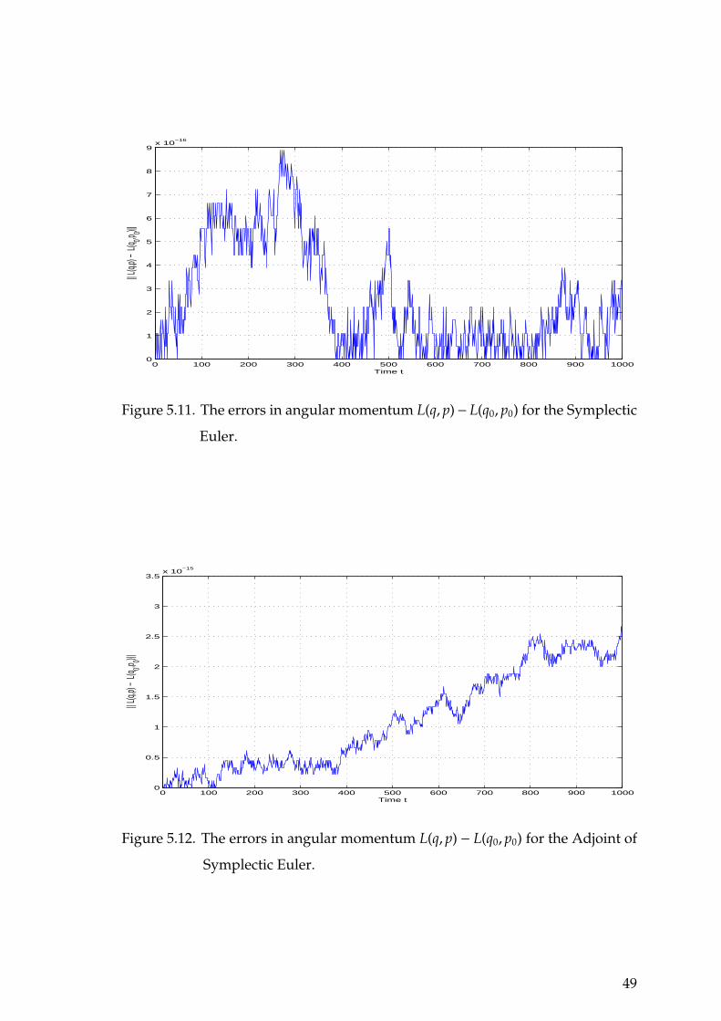
0 100 200 300 400 500 600 700 800 900 10000
1
2
3
4
5
6
7
8
9x 10
−16
Time t
|| L(q,
p) −
L(q0,p 0)||
Figure 5.11. The errors in angular momentum L(q, p)− L(q0, p0) for the Symplectic
Euler.
0 100 200 300 400 500 600 700 800 900 10000
0.5
1
1.5
2
2.5
3
3.5x 10
−15
Time t
|| L(q,
p) −
L(q0,p 0)||
Figure 5.12. The errors in angular momentum L(q, p) − L(q0, p0) for the Adjoint of
Symplectic Euler.
49

5.1.4. Conservation of Runge-Lenz Vector
Conservation of Runge-Lenz vector is presented in Figure(5.13, 5.14, 5.15,
5.16) by explicit Euler, implicit Euler, symplectic Euler and adjoint of symplectic
Euler, respectively. It can be seen in these figures that symplectic methods preserve
this quantity better than explicit and implicit Euler method.
0 1000 2000 3000 4000 5000 6000 7000 8000 9000 100000
0.1
0.2
0.3
0.4
0.5
0.6
0.7
0.8
0.9
Time t
|| A(q,
p) −
A(q0,p 0)||
Figure 5.13. The errors in Runge-Lenz vector A(q, p) − A(q0, p0) for the Explicit
Euler.
0 100 200 300 400 500 600 700 800 900 10000
0.05
0.1
0.15
0.2
0.25
0.3
0.35
0.4
0.45
Time t
|| A(q,
p) −
A(q0,p 0)||
Figure 5.14. The errors in Runge-Lenz vector A(q, p) − A(q0, p0) for the Implicit
Euler .
50

0 100 200 300 400 500 600 700 800 900 10000.05
0.1
0.15
0.2
0.25
0.3
0.35
0.4
0.45
0.5
0.55
Time t
|| A(q,
p) −
A(q 0,p 0)||
Figure 5.15. The errors in Runge-Lenz vector A(q, p) −A(q0, p0) for the Symplectic
Euler.
0 100 200 300 400 500 600 700 800 900 10000.05
0.1
0.15
0.2
0.25
0.3
0.35
0.4
0.45
0.5
0.55
Time t
|| A(q,
p) −
A(q 0,p 0)||
Figure 5.16. The errors in Runge-Lenz vector A(q, p) − A(q0, p0) for the Adjoint of
Symplectic Euler.
51

5.2. Second Order Methods
In this section we consider second order methods, namely, trapezoidal rule,
implicit midpoint rule and Stormer-Verlet method.
5.2.1. Phase Spaces
In this subsection we obtain trajectory of motion by using trapezoidal
rule, implicit midpoint rule and Stormer-Verlet method. Figure(5.17) presents the
trajectory of motion obtained by trapezoidal rule. It can be easily seen that the
trajectory of motion gets deformed. Since trapezoidal rule is a non-geometric
integrator we could not obtain closed curves. Figure(5.18) and Figure(5.19) show
the phase space of the Kepler problem obtained by implicit midpoint and Stormer-
Verlet method, respectively. Since both of these methods are symplectic geometric
integrators the shape of the trajectory preserved by both these methods.
−1−0.5
00.5
11.5
2
−1.5
−1
−0.5
0
0.5
1−1
−0.5
0
0.5
1
1.5
q1q2
q3
Figure 5.17. Trajectory of motion by Trapezoidal Rule.
52

−1−0.5
00.5
11.5
2
−1.5
−1
−0.5
0
0.5
1−1
−0.5
0
0.5
1
1.5
2
q1q2
q3
Figure 5.18. Trajectory of motion by Midpoint Rule.
−1−0.5
00.5
11.5
2
−1.5
−1
−0.5
0
0.5
1−1
−0.5
0
0.5
1
1.5
2
q1q2
q3
Figure 5.19. Trajectory of motion by Stormer-Verlet scheme.
53

5.2.2. Conservation of Energy
Figure(5.20, 5.21, 5.22) present conservation of the energy by trapezoidal
rule, implicit midpoint rule and Stormer-Verlet method, respectively. We
observed the following: implicit midpoint rule and Stormer-Verlet method
conserved the energy since they are symplectic geometric integration methods.
Conservation of the energy by these methods is better than trapezoidal rule.
0 100 200 300 400 500 600 700 800 900 1000−0.05
−0.04
−0.03
−0.02
−0.01
0
0.01
Time t
H(q,p
) − H
(q 0,p 0)
Figure 5.20. The errors in Hamiltonian H(q, p)−H(q0, p0) for the Trapezoidal Rule.
54

0 10 20 30 40 50 60 70 80 90 100−2
0
2
4
6
8
10
12x 10
−3
Time t
H(q,p
) − H
(q 0,p 0)
Figure 5.21. The errors in Hamiltonian H(q, p) −H(q0, p0) for Midpoint Rule.
0 10 20 30 40 50 60 70 80 90 100−9
−8
−7
−6
−5
−4
−3
−2
−1
0
1x 10
−3
Time t
H(q,p
) − H
(q 0,p 0)
Figure 5.22. The errors in Hamiltonian H(q, p)−H(q0, p0) for Stormer-Verlet scheme.
55

5.2.3. Conservation of Angular Momentum
Error in angular momentum is shown in Figure(5.23, 5.24, 5.25) by
trapezoidal rule, implicit midpoint rule and Stormer-Verlet method, respectively.
Angular momentum is conserved by midpoint rule and Stormer-Verlet method
up to the computer accuracy. Implicit midpoint rule and Stormer-Verlet method
conserve this quantity better than trapezoidal rule.
0 100 200 300 400 500 600 700 800 900 10000
0.005
0.01
0.015
0.02
0.025
0.03
Time t
|| L(q,
p) −
L(q0,p 0)||
Figure 5.23. The errors in angular momentum L(q, p) − L(q0, p0) for Trapezoidal
rule.
56

0 10 20 30 40 50 60 70 80 90 1000
0.2
0.4
0.6
0.8
1
1.2
1.4
1.6x 10
−15
Time t
|| L(q,
p) −
L(q0,p 0)||
Figure 5.24. The errors in angular momentum L(q, p) − L(q0, p0) Midpoint Rule.
0 100 200 300 400 500 600 700 800 900 10000
0.5
1
1.5
2
2.5
3
3.5
4x 10
−15
Time t
|| L(q,
p) −
L(q0,p 0)||
Figure 5.25. The errors in angular momentum L(q, p)− L(q0, p0) for Stormer-Verlet
scheme.
57

5.2.4. Conservation of Runge-Lenz Vector
Conservation of Runge-Lenz vector is shown in Figure(5.26, 5.27, 5.28) by
trapezoidal rule, implicit midpoint rule and Stormer-Verlet method, respectively.
As can be seen in these figures that implicit midpoint rule and Stormer-Verlet
method preserve the Runge-Lenz vector better than trapezoidal rule.
0 100 200 300 400 500 600 700 800 900 10000
0.1
0.2
0.3
0.4
0.5
0.6
0.7
0.8
0.9
Time t
|| A(q,
p) −
A(q 0,p 0)||
Figure 5.26. The errors in Runge-Lenz vector A(q, p)−A(q0, p0) for the Trapezoidal
rule.
58

0 10 20 30 40 50 60 70 80 90 1000
0.05
0.1
0.15
0.2
0.25
0.3
0.35
Time t
|| A(q,
p) −
A(q 0,p 0)||
Figure 5.27. The errors in Runge-Lenz vector A(q, p)−A(q0, p0) for Midpoint Rule.
0 10 20 30 40 50 60 70 80 90 1000
0.02
0.04
0.06
0.08
0.1
0.12
0.14
Time t
|| A(q,
p) −
A(q 0,p 0)||
Figure 5.28. The errors in Runge-Lenz vector A(q, p) −A(q0, p0) for Stormer-Verlet
scheme.
59

5.3. Third Order Methods
In this section classic 3rd order Runge-Kutta method as we mention in
section 3.4 and composition methods of order 3 are considered as third order
methods. In composition methods we use midpoint rule and Stormer-Verlet
method as the base methods such that let Φh be our base method and γ1 = γ3 =
12−2(1/3) , γ2 = − 2(1/3)
2−2(1/3) real numbers. Its composition with step sizes γ1h, γ2h, γ3h
i.e.,
Ψh = Φγ3h o Φγ2h o Φγ1h
is the corresponding composition method (Hairer, et al. 2001).
5.3.1. Phase Spaces
In this subsection trajectory of motion obtained by classic 3rd order Runge-
Kutta method can be seen in Figure(5.29). Since 3rd order Runge-Kutta method
is a non-geometric integrator we could not obtain closed curves. Figure(5.30) and
Figure(5.31) present the trajectory of motion obtained by composition method
of order 3 (midpoint rule as base method) and composition method of order 3
(Stormer-Verlet as base method), respectively. Since composition of symplectic
method is symplectic method the shape of the trajectory preserved by this method.
−1.5−1
−0.50
0.51
−1
−0.5
0
0.5
1
1.5
2−0.4
−0.2
0
0.2
0.4
0.6
0.8
1
1.2
q1q2
q3
Figure 5.29. Trajectory of motion by 3rd order Runge-Kutta.
60

−1−0.5
00.5
11.5
2
−1
−0.5
0
0.5
1
1.5−0.8
−0.6
−0.4
−0.2
0
0.2
0.4
0.6
0.8
q1q2
q3
Figure 5.30. Trajectory of motion by Composition method of order 3 (midpoint
rule as base method).
−0.8−0.6
−0.4−0.2
00.2
0.40.6
−0.4
−0.2
0
0.2
0.4
0.6−0.4
−0.3
−0.2
−0.1
0
0.1
0.2
0.3
q1
q2
q 3
Figure 5.31. Trajectory of motion by Composition method of order 3 (Stormer-
Verlet as base method).
61
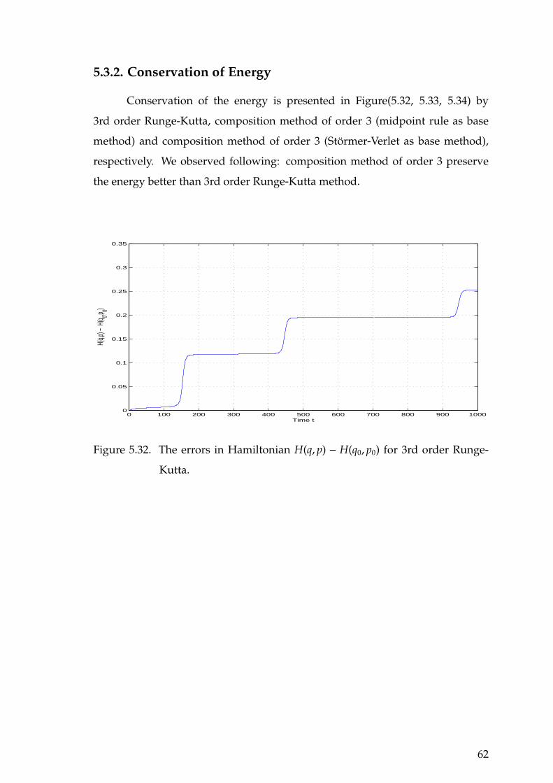
5.3.2. Conservation of Energy
Conservation of the energy is presented in Figure(5.32, 5.33, 5.34) by
3rd order Runge-Kutta, composition method of order 3 (midpoint rule as base
method) and composition method of order 3 (Stormer-Verlet as base method),
respectively. We observed following: composition method of order 3 preserve
the energy better than 3rd order Runge-Kutta method.
0 100 200 300 400 500 600 700 800 900 10000
0.05
0.1
0.15
0.2
0.25
0.3
0.35
Time t
H(q,p
) − H
(q 0,p 0)
Figure 5.32. The errors in Hamiltonian H(q, p) − H(q0, p0) for 3rd order Runge-
Kutta.
62

0 10 20 30 40 50 60 70 80 90 100−1
0
1
2
3
4
5
6
7x 10
−3
Time t
H(q,p
) − H
(q 0,p 0)
Figure 5.33. The errors in Hamiltonian H(q, p)−H(q0, p0) for Composition method
of order 3 (midpoint rule as base method).
0 100 200 300 400 500 600 700 800 900 10000
0.5
1
1.5
2
2.5
3
3.5x 10
−4
Figure 5.34. The errors in Hamiltonian H(q, p)−H(q0, p0) for Composition method
of order 3 (Stormer-Verlet as base method).
63
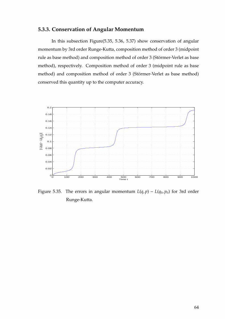
5.3.3. Conservation of Angular Momentum
In this subsection Figure(5.35, 5.36, 5.37) show conservation of angular
momentum by 3rd order Runge-Kutta, composition method of order 3 (midpoint
rule as base method) and composition method of order 3 (Stormer-Verlet as base
method), respectively. Composition method of order 3 (midpoint rule as base
method) and composition method of order 3 (Stormer-Verlet as base method)
conserved this quantity up to the computer accuracy.
0 100 200 300 400 500 600 700 800 900 10000
0.02
0.04
0.06
0.08
0.1
0.12
0.14
0.16
0.18
0.2
Time t
|| L(q,
p) −
L(q0,p 0)||
Figure 5.35. The errors in angular momentum L(q, p) − L(q0, p0) for 3rd order
Runge-Kutta.
64

0 10 20 30 40 50 60 70 80 90 1000
0.2
0.4
0.6
0.8
1
1.2x 10
−15
Time t
|| L(q,
p) −
L(q0,p 0)||
Figure 5.36. The errors in angular momentum L(q, p) − L(q0, p0) Composition
method of order 3 (midpoint rule as base method).
0 100 200 300 400 500 600 700 800 900 10000
0.5
1
1.5
2
2.5
3
3.5
4
4.5
5x 10
−15
Figure 5.37. The errors in angular momentum L(q, p) − L(q0, p0) Composition
method of order 3 (Stormer-Verlet as base method).
65
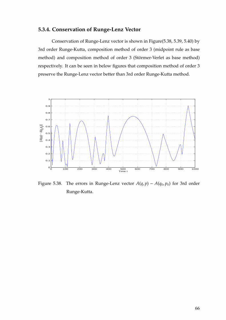
5.3.4. Conservation of Runge-Lenz Vector
Conservation of Runge-Lenz vector is shown in Figure(5.38, 5.39, 5.40) by
3rd order Runge-Kutta, composition method of order 3 (midpoint rule as base
method) and composition method of order 3 (Stormer-Verlet as base method)
respectively. It can be seen in below figures that composition method of order 3
preserve the Runge-Lenz vector better than 3rd order Runge-Kutta method.
0 100 200 300 400 500 600 700 800 900 10000
0.1
0.2
0.3
0.4
0.5
0.6
0.7
0.8
0.9
1
Time t
|| A(q,
p) −
A(q 0,p 0)||
Figure 5.38. The errors in Runge-Lenz vector A(q, p) − A(q0, p0) for 3rd order
Runge-Kutta.
66

0 10 20 30 40 50 60 70 80 90 1000
0.02
0.04
0.06
0.08
0.1
0.12
0.14
Time t
|| A(q,
p) −
A(q 0,p 0)||
Figure 5.39. The errors in Runge-Lenz vector A(q, p) − A(q0, p0) for Composition
method of order 3 (midpoint rule as base method).
0 100 200 300 400 500 600 700 800 900 10000
0.1
0.2
0.3
0.4
0.5
0.6
0.7
0.8
Figure 5.40. The errors in Runge-Lenz vector A(q, p) − A(q0, p0) for Composition
method of order 3 (Stormer-Verlet as base method).
67

5.4. Fourth and Fifth Order Methods
In this section we consider fourth and fifth order methods, namely, classic
4th order Runge-Kutta method that we mentioned in chapter 3.4 and composition
methods of order 5. In composition methods we use midpoint rule and Stormer-
Verlet method as base methods. In composition methods we use step sizes γ1 =
γ2 = γ4 = γ5 = γ1 = 14−4(1/5) and γ3 = − 4(1/5)
4−4(1/5) .
5.4.1. Phase Spaces
In this subsection trajectory of motion obtained by classic 4th order Runge-
Kutta method is shown in Figure(5.41). Since 4th order Runge-Kutta is a non-
geometric integrator we could not obtain closed curves. Figure(5.42) and Fig-
ure(5.43) present trajectory of motion obtained by composition method of order
5 (midpoint rule as base method) and composition method of order 5 (Stormer-
Verlet as base method), respectively. Since composition method of order 5 are
symplectic geometric integrator the shape of the trajectory preserved by this
method.
−1.5−1
−0.50
0.51
−1
−0.5
0
0.5
1
1.5
2−0.4
−0.2
0
0.2
0.4
0.6
0.8
1
1.2
q1q2
q3
Figure 5.41. Trajectory of motion by 4th order Runge-Kutta.
68

−1−0.5
00.5
11.5
2
−1.5
−1
−0.5
0
0.5
1
1.5−1
−0.5
0
0.5
1
1.5
2
q1q2
q3
Figure 5.42. Trajectory of motion by Composition method of order 5 (midpoint
rule as base method).
−2−1.5
−1−0.5
00.5
11.5
−1
0
1
2
3
4−1.2
−1
−0.8
−0.6
−0.4
−0.2
0
0.2
0.4
0.6
q1
q2
q 3
Figure 5.43. Trajectory of motion by Composition method of order 5 (Stormer-
Verlet as base method).
69
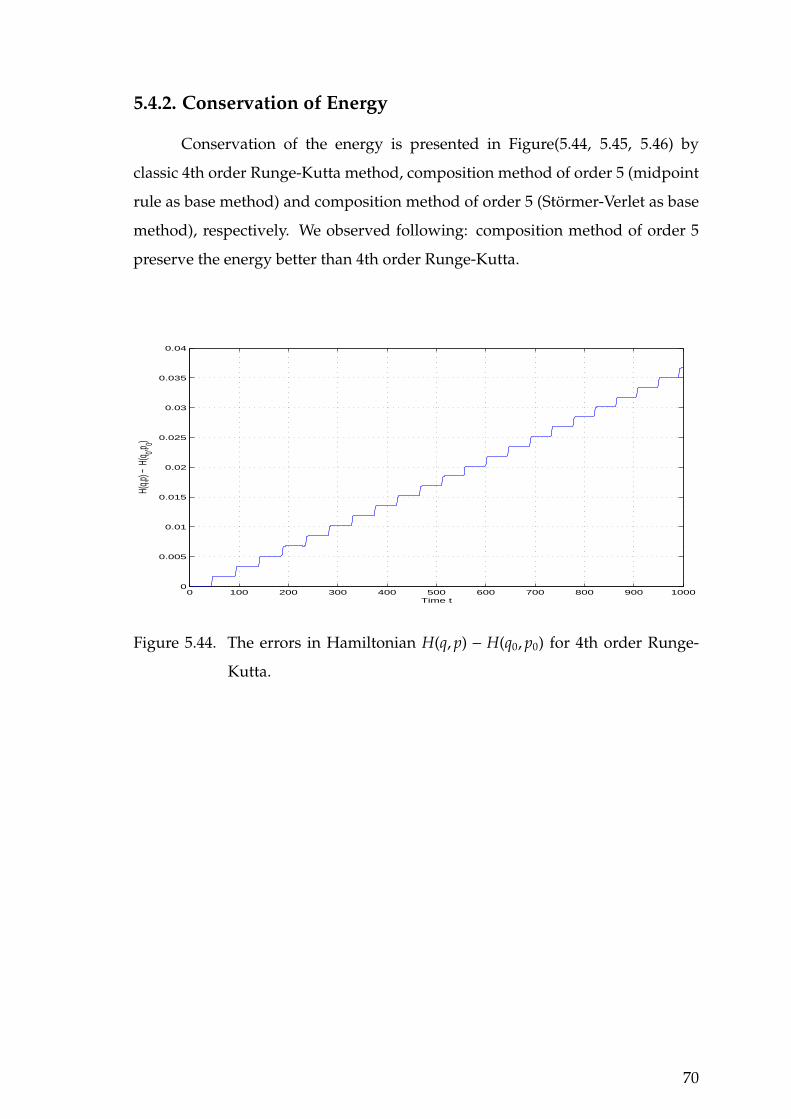
5.4.2. Conservation of Energy
Conservation of the energy is presented in Figure(5.44, 5.45, 5.46) by
classic 4th order Runge-Kutta method, composition method of order 5 (midpoint
rule as base method) and composition method of order 5 (Stormer-Verlet as base
method), respectively. We observed following: composition method of order 5
preserve the energy better than 4th order Runge-Kutta.
0 100 200 300 400 500 600 700 800 900 10000
0.005
0.01
0.015
0.02
0.025
0.03
0.035
0.04
Time t
H(q,p
) − H
(q 0,p 0)
Figure 5.44. The errors in Hamiltonian H(q, p) − H(q0, p0) for 4th order Runge-
Kutta.
70

0 10 20 30 40 50 60 70 80 90 100−2
0
2
4
6
8
10
12
14
16x 10
−4
Time t
H(q,p
) − H
(q 0,p 0)
Figure 5.45. The errors in Hamiltonian H(q, p)−H(q0, p0) for Composition method
of order 5 (midpoint rule as base method).
0 100 200 300 400 500 600 700 800 900 10000
1
x 10−4
Figure 5.46. The errors in Hamiltonian H(q, p)−H(q0, p0) for Composition method
of order 5 (Stormer-Verlet as base method).
71

5.4.3. Conservation of Angular Momentum
In this subsection conservation of angular momentum is shown in
Figure(5.47, 5.48, 5.49) by 4th order Runge-Kutta, composition method of
order 5 (midpoint rule as base method) and composition method of order 5
(Stormer-Verlet as base method), respectively. Composition method of order 5
conserved the angular momentum up to the computer accuracy. Conservation of
angular momentum by composition method of order 5 is better than 4th order
Runge-Kutta method.
0 100 200 300 400 500 600 700 800 900 10000
0.005
0.01
0.015
0.02
0.025
0.03
0.035
0.04
Time t
|| L(q,
p) −
L(q0,p 0)||
Figure 5.47. The errors in angular momentum L(q, p) − L(q0, p0) for 4th order
Runge-Kutta.
72

0 10 20 30 40 50 60 70 80 90 1000
0.5
1
1.5
2
2.5
3
3.5x 10
−15
Time t
|| L(q,
p) −
L(q0,p 0)||
Figure 5.48. The errors in angular momentum L(q, p) − L(q0, p0) Composition
method of order 5 (midpoint rule as base method).
0 100 200 300 400 500 600 700 800 900 10000
0.5
1
1.5
2
2.5
3
3.5x 10
−15
Figure 5.49. The errors in angular momentum L(q, p) − L(q0, p0) Composition
method of order 5 (Stormer-Verlet as base method).
73

5.4.4. Conservation of Runge-Lenz Vector
Conservation of Runge-Lenz vector is shown in Figure(5.50, 5.51, 5.52) by
4th order Runge-Kutta, composition method of order 5 (midpoint rule as base
method) and composition method of order 5 (Stormer-Verlet as base method),
respectively. We observe the following: composition method of order 5 preserve
the Runge-Lenz vector better than 4th order Runge-Kutta method.
0 100 200 300 400 500 600 700 800 900 10000
0.1
0.2
0.3
0.4
0.5
0.6
0.7
Time t
|| A(q,
p) −
A(q 0,p 0)||
Figure 5.50. The errors in Runge-Lenz vector A(q, p) − A(q0, p0) for 4th order
Runge-Kutta.
74

0 10 20 30 40 50 60 70 80 90 1000
0.002
0.004
0.006
0.008
0.01
0.012
Time t
|| A(q,
p) −
A(q 0,p 0)||
Figure 5.51. The errors in Runge-Lenz vector A(q, p) − A(q0, p0) for Composition
method of order 5 (midpoint rule as base method).
0 100 200 300 400 500 600 700 800 900 10000.1
0.2
0.3
0.4
0.5
0.6
0.7
0.8
0.9
Figure 5.52. The errors in Runge-Lenz vector A(q, p) − A(q0, p0) for Composition
method of order 5 (Stormer-Verlet as base method).
75

CHAPTER 6
SUMMARY AND CONCLUSION
In this thesis both geometric and non-geometric integration methods were
applied to the Kepler problem in order to determine which of its conserved
quantities were preserved better. For this purpose explicit Euler, implicit Euler,
symplectic Euler, adjoint of symplectic Euler, trapezoidal rule, midpoint rule,
Stormer-Verlet method, 3rd and 4th order Runge-Kutta methods were chosen. In
addition we constructed higher order symplectic method by composition tech-
niques considering midpoint rule and Stormer-Verlet method as base methods.
All algorithms of the methods were written in MATLAB.
The results obtained from computations are summarized in Table (1). In
this table norm of errors in energy, angular momentum, Runge-Lenz vector and
CPU times of the methods that we mentioned above are presented. From the table
the following results are relived:
• Implicit methods are more expensive than explicit methods.
• Symplectic methods conserved three quantities of the Kepler problem better.
• When the order of the methods increase we get better conservation of the
quantities.
• The best conservation of the quantities is obtained by composition method of
order 5 (midpoint as the base method) however it’s the most expensive method.
• In general the Runge-Lenz vector is not conserved by any method in a higher
accuracy.
76
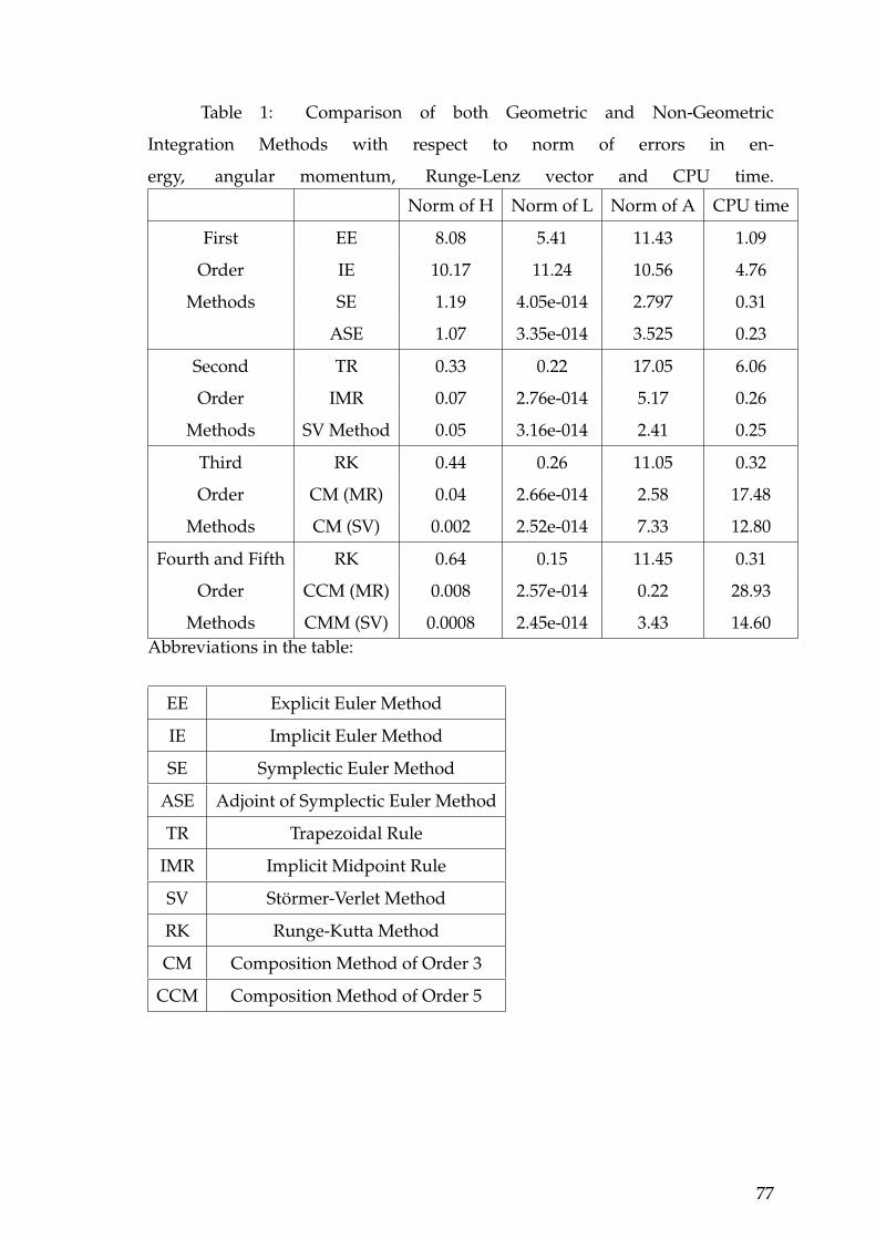
Table 1: Comparison of both Geometric and Non-Geometric
Integration Methods with respect to norm of errors in en-
ergy, angular momentum, Runge-Lenz vector and CPU time.
Norm of H Norm of L Norm of A CPU time
First EE 8.08 5.41 11.43 1.09
Order IE 10.17 11.24 10.56 4.76
Methods SE 1.19 4.05e-014 2.797 0.31
ASE 1.07 3.35e-014 3.525 0.23
Second TR 0.33 0.22 17.05 6.06
Order IMR 0.07 2.76e-014 5.17 0.26
Methods SV Method 0.05 3.16e-014 2.41 0.25
Third RK 0.44 0.26 11.05 0.32
Order CM (MR) 0.04 2.66e-014 2.58 17.48
Methods CM (SV) 0.002 2.52e-014 7.33 12.80
Fourth and Fifth RK 0.64 0.15 11.45 0.31
Order CCM (MR) 0.008 2.57e-014 0.22 28.93
Methods CMM (SV) 0.0008 2.45e-014 3.43 14.60Abbreviations in the table:
EE Explicit Euler Method
IE Implicit Euler Method
SE Symplectic Euler Method
ASE Adjoint of Symplectic Euler Method
TR Trapezoidal Rule
IMR Implicit Midpoint Rule
SV Stormer-Verlet Method
RK Runge-Kutta Method
CM Composition Method of Order 3
CCM Composition Method of Order 5
77
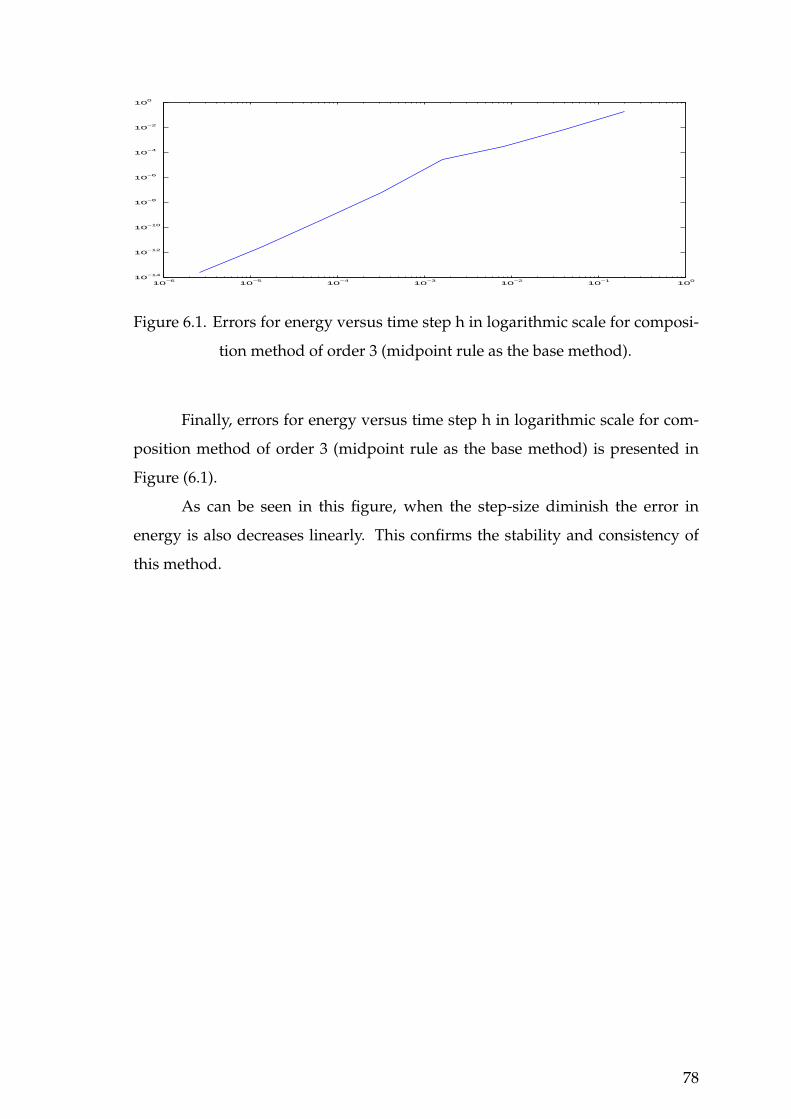
10−6
10−5
10−4
10−3
10−2
10−1
100
10−14
10−12
10−10
10−8
10−6
10−4
10−2
100
Figure 6.1. Errors for energy versus time step h in logarithmic scale for composi-
tion method of order 3 (midpoint rule as the base method).
Finally, errors for energy versus time step h in logarithmic scale for com-
position method of order 3 (midpoint rule as the base method) is presented in
Figure (6.1).
As can be seen in this figure, when the step-size diminish the error in
energy is also decreases linearly. This confirms the stability and consistency of
this method.
78

REFERENCES
Budd C.J. and Iserles A., 1999. Geometric Integration: Numerical Solutions ofDifferential Equations. Phil. Trans. Roy. Soc. A 357: 943-1133.
Budd C.J. and Piggott M.D., 2000. Geometric Integration and Its Applications. Inhandbook of Numerical Analysis: 35-139.
Butcher J.C., 1987. The Numerical Analysis of Ordinary Differential Equations,RungeKutta and General Linear Methods. A Wiley- Interscience Publication. JohnWiley and Sons Ltd.
Hairer E., 2005. Important Aspects of Geometric Numerical Integration. Journal ofScientific Computing: 67-81.
Hairer E., Lubich C.,Wanner G., eds. 2001. Geometric Numerical Integration. Berlin:Springer Series in Computational Mathematics.
Hairer E., Lubich C.,Wanner G., eds. 2006. Geometric Numerical Integration.Structure-preserving algorithms for ordinary differential equations. Springer-Verlag,Berlin : Second edition.
Kozlov R., 2007. Conservative Discritizations of the Kepler Problem. Journal ofPhysics A: Mathematical and Theoretical: 4529-4539.
Leimkuhler B. and Reich S., 2004. Simulating Hamiltonian Dynamics. USA : Cam-bridge University Press.
Rama Mohana Rao M., 1979. Ordinary Differential Equations.Theory and Applications.Indiana: Adword Arnold.
McLachlan R., 2004. Geometric Integrators for ODE’s. Australia: Australian Re-search Council.
McLachlan R.,Quispel W., 2005. Geometric integrators for ODEs. J. Phys. A: Math.Gen. 39: 5251-5285.
McLachlan R. and Quispel W., 1999. Six lectures on the geometric integration ofODEs. In Foundations of Computational Mathematics (Oxford, 1999): 155-210.
Sanz Serna J.M. 1994. Numerical Hamiltonian Problems. London: Applied mathe-matics and mathematical computation.
Stuart A.M., Humphries A. R., 1996. Dynamical Systems and Numerical Analysis.USA : Cambridge University Press.
Quispel G.R.W. and Dyt C., 1997. Solving ODE’s Numerically while PreservingSymmetries, Hamiltonian Structure, Phase Space Volume or First Integrals.Proc. 15th IMACS World Congress: 601-607.
79

APPENDIX A
MATLAB CODES
A.1. First Order Methods
A.1.1. Explicit Euler
N = 1000;
h = 100/N ;
K = 1;
%initial conditions
q0 = [ 0.8 , 0.6 , 0 ]’ ;
p0 = [ 0 , 1 , 0.5 ]’ ;
r0 = sqrt( q0’*q0) ;
q1 = q0 ;
p1 = p0 ;
r1 = sqrt( q1’*q1) ;
%first energy
H0 = ( ( p1’*p1/2 ) - ( K /r1 ) );
%for angular momentum
m1 = q1(2)*p1(3) - q1(3)*p1(2);
m2 = q1(3)*p1(1) - q1(1)*p1(3);
m3 = q1(1)*p1(2) - q1(2)*p1(1);
%first angular momentum
L0 = [ m1 , m2 , m3 ]’ ;
%first Runge-Lenz vector
RL0 = q1 *(H0 + p1’*p1/2 ) - p1 *(q1’*p1) ;
% computational unit
80
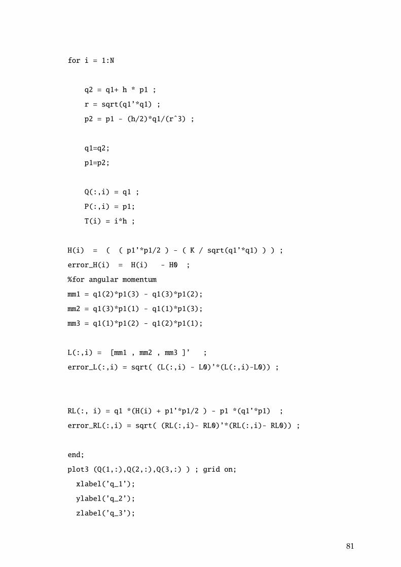
for i = 1:N
q2 = q1+ h * p1 ;
r = sqrt(q1’*q1) ;
p2 = p1 - (h/2)*q1/(rˆ3) ;
q1=q2;
p1=p2;
Q(:,i) = q1 ;
P(:,i) = p1;
T(i) = i*h ;
H(i) = ( ( p1’*p1/2 ) - ( K / sqrt(q1’*q1) ) ) ;
error_H(i) = H(i) - H0 ;
%for angular momentum
mm1 = q1(2)*p1(3) - q1(3)*p1(2);
mm2 = q1(3)*p1(1) - q1(1)*p1(3);
mm3 = q1(1)*p1(2) - q1(2)*p1(1);
L(:,i) = [mm1 , mm2 , mm3 ]’ ;
error_L(:,i) = sqrt( (L(:,i) - L0)’*(L(:,i)-L0)) ;
RL(:, i) = q1 *(H(i) + p1’*p1/2 ) - p1 *(q1’*p1) ;
error_RL(:,i) = sqrt( (RL(:,i)- RL0)’*(RL(:,i)- RL0)) ;
end;
plot3 (Q(1,:),Q(2,:),Q(3,:) ) ; grid on;
xlabel(’q_1’);
ylabel(’q_2’);
zlabel(’q_3’);
81

plot (T,error_H) ; grid on;
xlabel(’Time t’); ylabel(’H(q,p) - H(q_0,p_0)’);
plot (T,error_L) ; grid on;
xlabel(’Time t’); ylabel(’|| L(q,p) - L(q_0,p_0)||’);
plot (T,error_RL) ;grid on;
xlabel(’Time t’); ylabel(’|| A(q,p) - A(q_0,p_0)||’);
A.1.2. Implicit Euler
N = 1000;
h = 100/N ;
K = 1;
%initial conditions
q0 = [ 0.8 , 0.6 , 0 ]’ ;
p0 = [ 0 , 1 , 0.5 ]’ ;
r0 = sqrt( q0’*q0) ;
q = q0 ;
p = p0 ;
r = sqrt( q’*q) ;
%first energy
H0 = ( ( p’*p/2 ) - ( K /r ) );
%for angular momentum
m1 = q(2)*p(3) - q(3)*p(2);
m2 = q(3)*p(1) - q(1)*p(3);
m3 = q(1)*p(2) - q(2)*p(1);
%first angular momentum
L0 = [ m1 , m2 , m3 ]’ ;
%first Runge-Lenz vector
RL0 = q *(H0 + p’*p/2 ) - p *(q’*p) ;
82
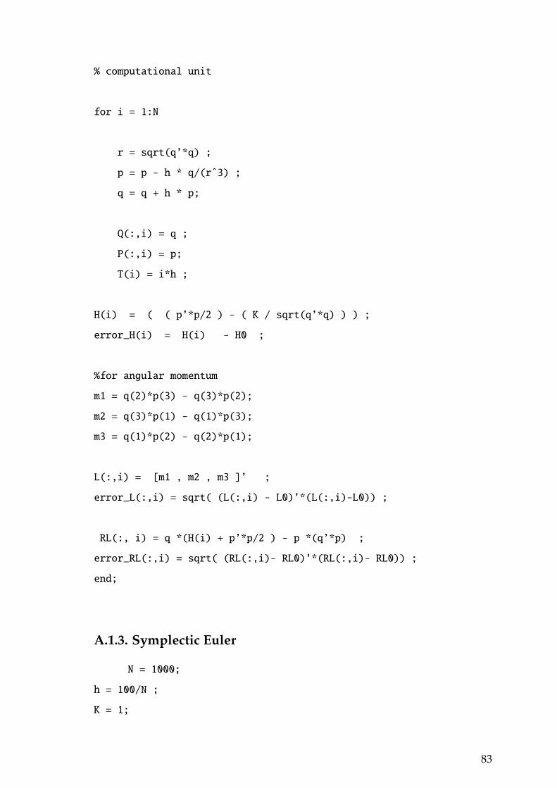
% computational unit
for i = 1:N
r = sqrt(q’*q) ;
p = p - h * q/(rˆ3) ;
q = q + h * p;
Q(:,i) = q ;
P(:,i) = p;
T(i) = i*h ;
H(i) = ( ( p’*p/2 ) - ( K / sqrt(q’*q) ) ) ;
error_H(i) = H(i) - H0 ;
%for angular momentum
m1 = q(2)*p(3) - q(3)*p(2);
m2 = q(3)*p(1) - q(1)*p(3);
m3 = q(1)*p(2) - q(2)*p(1);
L(:,i) = [m1 , m2 , m3 ]’ ;
error_L(:,i) = sqrt( (L(:,i) - L0)’*(L(:,i)-L0)) ;
RL(:, i) = q *(H(i) + p’*p/2 ) - p *(q’*p) ;
error_RL(:,i) = sqrt( (RL(:,i)- RL0)’*(RL(:,i)- RL0)) ;
end;
A.1.3. Symplectic Euler
N = 1000;
h = 100/N ;
K = 1;
83

%initial conditions
q0 = [ 0.8 , 0.6 , 0 ]’ ;
p0 = [ 0 , 1 , 0.5 ]’ ;
r0 = sqrt( q0’*q0) ;
q = q0 ;
p = p0 ;
r = sqrt( q’*q) ;
%first energy
H0 = ( ( p’*p/2 ) - ( K /r ) );
%for angular momentum
m1 = q(2)*p(3) - q(3)*p(2);
m2 = q(3)*p(1) - q(1)*p(3);
m3 = q(1)*p(2) - q(2)*p(1);
%first angular momentum
L0 = [ m1 , m2 , m3 ]’ ;
%first Runge-Lenz vector
RL0 = q *(H0 + p’*p/2 ) - p *(q’*p) ;
% computational unit
for i = 1:N
q = q + h * p;
r = sqrt(q’*q) ;
p = p - h * q/(rˆ3) ;
Q(:,i) = q ;
P(:,i) = p;
T(i) = i*h ;
H(i) = ( ( p’*p/2 ) - ( K / sqrt(q’*q) ) ) ;
84
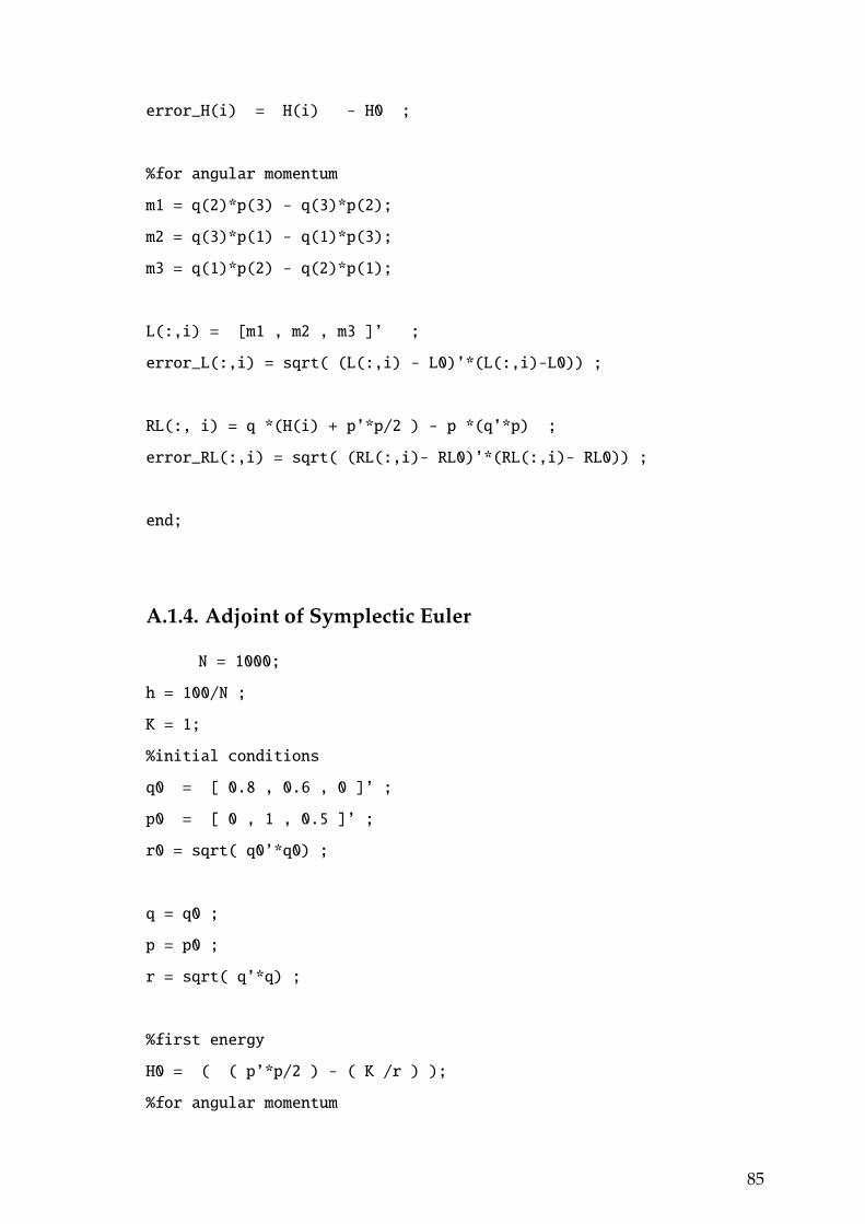
error_H(i) = H(i) - H0 ;
%for angular momentum
m1 = q(2)*p(3) - q(3)*p(2);
m2 = q(3)*p(1) - q(1)*p(3);
m3 = q(1)*p(2) - q(2)*p(1);
L(:,i) = [m1 , m2 , m3 ]’ ;
error_L(:,i) = sqrt( (L(:,i) - L0)’*(L(:,i)-L0)) ;
RL(:, i) = q *(H(i) + p’*p/2 ) - p *(q’*p) ;
error_RL(:,i) = sqrt( (RL(:,i)- RL0)’*(RL(:,i)- RL0)) ;
end;
A.1.4. Adjoint of Symplectic Euler
N = 1000;
h = 100/N ;
K = 1;
%initial conditions
q0 = [ 0.8 , 0.6 , 0 ]’ ;
p0 = [ 0 , 1 , 0.5 ]’ ;
r0 = sqrt( q0’*q0) ;
q = q0 ;
p = p0 ;
r = sqrt( q’*q) ;
%first energy
H0 = ( ( p’*p/2 ) - ( K /r ) );
%for angular momentum
85
m1 = q(2)*p(3) - q(3)*p(2);
m2 = q(3)*p(1) - q(1)*p(3);
m3 = q(1)*p(2) - q(2)*p(1);
%first angular momentum
L0 = [ m1 , m2 , m3 ]’ ;
%first Runge-Lenz vector
RL0 = q *(H0 + p’*p/2 ) - p *(q’*p) ;
% computational unit
for i = 1:N
r = sqrt(q’*q) ;
p = p - h * q/(rˆ3) ;
q = q + h * p;
Q(:,i) = q ;
P(:,i) = p;
T(i) = i*h ;
H(i) = ( ( p’*p/2 ) - ( K / sqrt(q’*q) ) ) ;
error_H(i) = H(i) - H0 ;
%for angular momentum
m1 = q(2)*p(3) - q(3)*p(2);
m2 = q(3)*p(1) - q(1)*p(3);
m3 = q(1)*p(2) - q(2)*p(1);
L(:,i) = [m1 , m2 , m3 ]’ ;
error_L(:,i) = sqrt( (L(:,i) - L0)’*(L(:,i)-L0)) ;
86

RL(:, i) = q *(H(i) + p’*p/2 ) - p *(q’*p) ;
error_RL(:,i) = sqrt( (RL(:,i)- RL0)’*(RL(:,i)- RL0)) ;
end;
A.2. Second Order Methods
A.2.1. Trapezoidal Rule
N = 1000 % 752;
h = 0.15 ;
K = 1;
x0 = [ 0.8 , 0.6 , 0 ]’ ;
p0 = [ 0 , 1 , 0.5 ]’ ;
t0 = 0 ;
r0 = sqrt( x0’*x0) ;
x = x0 ;
p = p0 ;
r = sqrt( x’*x) ;
H0 = ( ( p’*p/2 ) - ( K /r ) )
m12 = x(1)*p(2) - x(2)*p(1);
m13 = x(1)*p(3) - x(3)*p(1);
m23 = x(2)*p(3) - x(3)*p(2);
M0 = [ m12 , m13 , m23 ]’ ;
RL0 = x *(H0 + p’*p/2 ) - p *(x’*p) ;
% computational unit
87
for i = 1:N
x1 = x ;
p1 = p;
x2 = x1 ;
p2 = p1;
for k = 1:100
p_mid = (p+p1)/2;
x2 = x + h * p_mid ;
r1 = sqrt( x1’*x1) ;
r2= sqrt( x’*x) ;
p2 = p - h/2*K*(x1/(r1ˆ3) + x/(r2ˆ3) ) ;
x1= x2;
p1 = p2;
end;
X(:,i) = x1 ;
P(:,i) = p1;
T(i) = i*h ;
x = x1;
p = p1;
H(i) = ( ( p’*p/2 ) - ( K / sqrt(x’*x) ) ) ;
error_H(i) = H(i) - H0 ;
m12 = x(1)*p(2) - x(2)*p(1);
88

m13 = x(1)*p(3) - x(3)*p(1);
m23 = x(2)*p(3) - x(3)*p(2);
M(:,i) = [m12 , m13 , m23 ]’ ;
error_M(:,i) = sqrt( (M(:,i) - M0)’*(M(:,i)-M0)) ;
RL(:, i) = x *(H(i) + p’*p/2 ) - p *(x’*p) ;
error_RL(:,i) = sqrt( (RL(:,i)- RL0)’*(RL(:,i)- RL0)) ;
end;
A.2.2. Midpoint Rule
N = 1000;
h = 100/N ;
K = 1;
%initial conditions
q0 = [ 0.8 , 0.6 , 0 ]’ ;
p0 = [ 0 , 1 , 0.5 ]’ ;
r0 = sqrt( q0’*q0) ;
q = q0 ;
p = p0 ;
r = sqrt( q’*q) ;
%first energy
H0 = ( ( p’*p/2 ) - ( K /r ) );
%for angular momentum
m1 = q(2)*p(3) - q(3)*p(2);
m2 = q(3)*p(1) - q(1)*p(3);
m3 = q(1)*p(2) - q(2)*p(1);
%first angular momentum
L0 = [ m1 , m2 , m3 ]’ ;
%first Runge-Lenz vector
RL0 = q *(H0 + p’*p/2 ) - p *(q’*p) ;
% computational unit
89

for i = 1:N
q1 = q ;
p1 = p;
q2 = q1 ;
p2 = p1;
for k = 1:100
p_mid = (p+p1)/2;
q2 = q + h * p_mid ;
q_mid = (q+q1)/2;
r = sqrt( q_mid’*q_mid) ;
p2 = p - h*K*q_mid/(rˆ3) ;
q1= q2;
p1 = p2;
end;
Q(:,i) = q1 ;
P(:,i) = p1;
T(i) = i*h ;
q = q1;
p = p1;
H(i) = ( ( p’*p/2 ) - ( K / sqrt(q’*q) ) ) ;
error_H(i) = H(i) - H0 ;
%for angular momentum
90

m1 = q(2)*p(3) - q(3)*p(2);
m2 = q(3)*p(1) - q(1)*p(3);
m3 = q(1)*p(2) - q(2)*p(1);
L(:,i) = [m1 , m2 , m3 ]’ ;
error_L(:,i) = sqrt( (L(:,i) - L0)’*(L(:,i)-L0)) ;
RL(:, i) = q *(H(i) + p’*p/2 ) - p *(q’*p) ;
error_RL(:,i) = sqrt( (RL(:,i)- RL0)’*(RL(:,i)- RL0)) ;
end;
A.2.3. Stormer-Verlet Method
N = 1000;
h = 100/N ;
K = 1;
%initial conditions
q0 = [ 0.8 , 0.6 , 0 ]’ ;
p0 = [ 0 , 1 , 0.5 ]’ ;
r0 = sqrt( q0’*q0) ;
q = q0 ;
p = p0 ;
r = sqrt( q’*q) ;
%first energy
H0 = ( ( p’*p/2 ) - ( K /r ) );
%for angular momentum
m1 = q(2)*p(3) - q(3)*p(2);
m2 = q(3)*p(1) - q(1)*p(3);
m3 = q(1)*p(2) - q(2)*p(1);
91

%first angular momentum
L0 = [ m1 , m2 , m3 ]’ ;
%first Runge-Lenz vector
RL0 = q *(H0 + p’*p/2 ) - p *(q’*p) ;
% computational unit
for i = 1:N
r = sqrt(q’*q) ;
x = p - (h/2)*q/(rˆ3) ;
q = q + h * x ;
r = sqrt(q’*q) ;
p = x - (h/2)*q/(rˆ3) ;
Q(:,i) = q ;
P(:,i) = p;
T(i) = i*h ;
H(i) = ( ( p’*p/2 ) - ( K / sqrt(q’*q) ) ) ;
error_H(i) = H(i) - H0 ;
%for angular momentum
m1 = q(2)*p(3) - q(3)*p(2);
m2 = q(3)*p(1) - q(1)*p(3);
m3 = q(1)*p(2) - q(2)*p(1);
L(:,i) = [m1 , m2 , m3 ]’ ;
error_L(:,i) = sqrt( (L(:,i) - L0)’*(L(:,i)-L0)) ;
RL(:, i) = q *(H(i) + p’*p/2 ) - p *(q’*p) ;
92
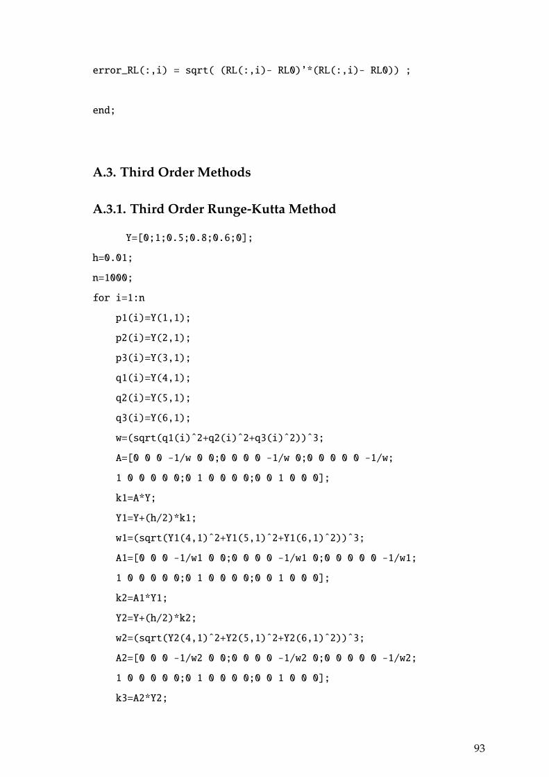
error_RL(:,i) = sqrt( (RL(:,i)- RL0)’*(RL(:,i)- RL0)) ;
end;
A.3. Third Order Methods
A.3.1. Third Order Runge-Kutta Method
Y=[0;1;0.5;0.8;0.6;0];
h=0.01;
n=1000;
for i=1:n
p1(i)=Y(1,1);
p2(i)=Y(2,1);
p3(i)=Y(3,1);
q1(i)=Y(4,1);
q2(i)=Y(5,1);
q3(i)=Y(6,1);
w=(sqrt(q1(i)ˆ2+q2(i)ˆ2+q3(i)ˆ2))ˆ3;
A=[0 0 0 -1/w 0 0;0 0 0 0 -1/w 0;0 0 0 0 0 -1/w;
1 0 0 0 0 0;0 1 0 0 0 0;0 0 1 0 0 0];
k1=A*Y;
Y1=Y+(h/2)*k1;
w1=(sqrt(Y1(4,1)ˆ2+Y1(5,1)ˆ2+Y1(6,1)ˆ2))ˆ3;
A1=[0 0 0 -1/w1 0 0;0 0 0 0 -1/w1 0;0 0 0 0 0 -1/w1;
1 0 0 0 0 0;0 1 0 0 0 0;0 0 1 0 0 0];
k2=A1*Y1;
Y2=Y+(h/2)*k2;
w2=(sqrt(Y2(4,1)ˆ2+Y2(5,1)ˆ2+Y2(6,1)ˆ2))ˆ3;
A2=[0 0 0 -1/w2 0 0;0 0 0 0 -1/w2 0;0 0 0 0 0 -1/w2;
1 0 0 0 0 0;0 1 0 0 0 0;0 0 1 0 0 0];
k3=A2*Y2;
93

Y=Y+(1/6)*h*(k1+4*k2+2*k3);
L(i)=((q1(i)*p2(i)+q2(i)*p3(i)+q3(i)*p1(i))-
(q2(i)*p1(i)+q3(i)*p2(i)+q1(i)*p3(i)));
r(i)=abs(L(i)-L(1));
H(i)=0.5*((p1(i)).ˆ2+(p2(i)).ˆ2+(p3(i)).ˆ2)-1/
(sqrt((q1(i)).ˆ2+(q2(i)).ˆ2+(q3(i)).ˆ2));
e(i)=abs(H(i)-H(1));
H(1)=0.5*((p1(1)).ˆ2+(p2(1)).ˆ2+(p3(1)).ˆ2)-1/
(sqrt((q1(1)).ˆ2+(q2(1)).ˆ2+(q3(1)).ˆ2));
a=p1(1)*q1(1)+p2(1)*q2(1)+p3(1)*q3(1);
b=H(1)+(1/2)*sqrt((p1(1).ˆ2)+(p2(1).ˆ2)+(p3(1).ˆ2));
a1=(b*q1(1)-a*p1(1));
a2=(b*q2(1)-a*p2(1));
a3=(b*q3(1)-a*p3(1));
%Runge-Lenz vector
c=p1(i)*q1(i)+p2(i)*q2(i)+p3(i)*q3(i);
d=H(i)+(1/2)*sqrt((p1(i).ˆ2)+(p1(i).ˆ2)+(p1(i).ˆ2));
b1(i)=(d*q1(i)-c*p1(i));
b2(i)=(d*q2(i)-c*p2(i));
b3(i)=(d*q3(i)-c*p3(i));
R(i)=sqrt(((b1(i)-a1).ˆ2)+((b2(i)-a2).ˆ2)+((b3(i)-a3).ˆ2));
end
A.3.2. Composition Method of Order 3 (Midpoint as base method)
N = 1000;
h = 100/N ;
K = 1;
gama1=1/2-(2ˆ(1/3));
gama2=-((2ˆ(1/3))/2-(2ˆ(1/3)));
gama3=1/2-(2ˆ(1/3));
94

%initial conditions
q0 = [ 0.8 , 0.6 , 0 ]’ ;
p0 = [ 0 , 1 , 0.5 ]’ ;
r0 = sqrt( q0’*q0) ;
q1 = q0 ;
p1 = p0 ;
r1 = sqrt( q1’*q1) ;
%first energy
H0 = ( ( p1’*p1/2 ) - ( K /r1 ) );
%for angular momentum
m1 = q1(2)*p1(3) - q1(3)*p1(2);
m2 = q1(3)*p1(1) - q1(1)*p1(3);
m3 = q1(1)*p1(2) - q1(2)*p1(1);
%first angular momentum
L0 = [ m1 , m2 , m3 ]’ ;
%first Runge-Lenz vector
RL0 = q1 *(H0 + p1’*p1/2 ) - p1 *(q1’*p1) ;
% ----------------computational unit 1---------------
for i = 1:N
q11 = q1 ;
p11 = p1;
q21 = q11 ;
p21 = p11;
for k = 1:100
p_mid1 = (p1+p11)/2;
95

q21 = q1 + h *gama1* p_mid1 ;
q_mid1 = (q1+q11)/2;
r1 = sqrt( q_mid1’*q_mid1) ;
p21 = p1 - h*K*gama1*q_mid1/(r1ˆ3) ;
q11= q21;
p11 = p21;
end;
x1 = q11;
y1 = p11;
end;
%----------------computational unit 2------------------
q2 = x1 ;
p2 = y1 ;
r2 = sqrt( q2’*q2) ;
for i = 1:N
q12 = q2 ;
p12 = p2;
q22 = q12 ;
p22 = p12;
for k = 1:100
96
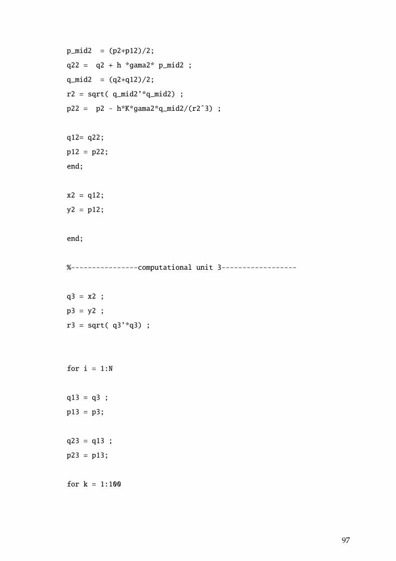
p_mid2 = (p2+p12)/2;
q22 = q2 + h *gama2* p_mid2 ;
q_mid2 = (q2+q12)/2;
r2 = sqrt( q_mid2’*q_mid2) ;
p22 = p2 - h*K*gama2*q_mid2/(r2ˆ3) ;
q12= q22;
p12 = p22;
end;
x2 = q12;
y2 = p12;
end;
%----------------computational unit 3------------------
q3 = x2 ;
p3 = y2 ;
r3 = sqrt( q3’*q3) ;
for i = 1:N
q13 = q3 ;
p13 = p3;
q23 = q13 ;
p23 = p13;
for k = 1:100
97

p_mid3 = (p3+p13)/2;
q23 = q3 + h *gama3* p_mid3 ;
q_mid3 = (q3+q13)/2;
r3 = sqrt( q_mid3’*q_mid3) ;
p23 = p3 - h*K*gama3*q_mid3/(r3ˆ3) ;
q13= q23;
p13 = p23;
end;
Q(:,i) = q13 ;
P(:,i) = p13;
T(i) = i*h ;
q3 = q13;
p3 = p13;
% energy
H(i) = ( ( p3’*p3/2 ) - ( K / sqrt(q3’*q3) ) ) ;
error_H(i) = H(i) - H0 ;
%angular momentum
mm1 = q3(2)*p3(3) - q3(3)*p3(2);
mm2 = q3(3)*p3(1) - q3(1)*p3(3);
mm3 = q3(1)*p3(2) - q3(2)*p3(1);
L(:,i) = [mm1 , mm2 , mm3 ]’ ;
error_L(:,i) = sqrt( (L(:,i) - L0)’*(L(:,i)-L0)) ;
%runge-lenz vector
98

RL(:, i) = q3 *(H(i) + p3’*p3/2 ) - p3 *(q3’*p3) ;
error_RL(:,i) = sqrt( (RL(:,i)- RL0)’*(RL(:,i)- RL0)) ;
end;
A.3.3. Composition Method of Order 3 (Stormer-Verlet as base
method)
q11(1)=0.8;
q21(1)=0.6;
p11(1)=0;
p21(1)=1;
q31(1)=0;
p31(1)=0.5;
h=0.01;
gama1=1/2-(2ˆ(1/3));
gama2=-((2ˆ(1/3))/2-(2ˆ(1/3)));
gama3=1/2-(2ˆ(1/3));h=0.007;
for i=1:1000;
k=p11(i)-(h/2)*gama1*(q11(i)/(q11(i).ˆ2+
q21(i).ˆ2+q31(i).ˆ2).ˆ(1.5));
m=p21(i)-(h/2)*gama1*(q21(i)/(q11(i).ˆ2+
q21(i).ˆ2+q31(i).ˆ2).ˆ(1.5));
t=p31(i)-(h/2)*gama1*(q31(i)/(q11(i).ˆ2+
q21(i).ˆ2+q31(i).ˆ2).ˆ(1.5));
q11(i+1)=q11(i)+h*gama1*k;
q21(i+1)=q21(i)+h*gama1*m;
q31(i+1)=q31(i)+h*gama1*t;
99
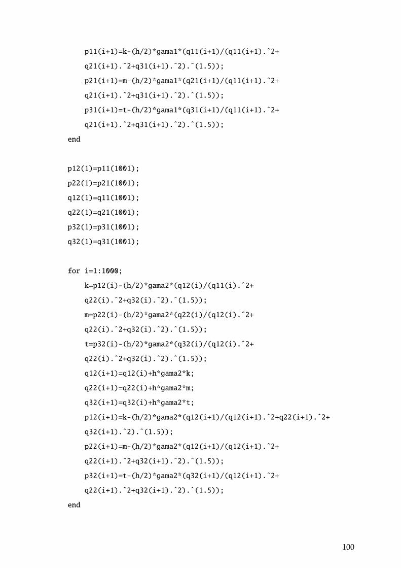
p11(i+1)=k-(h/2)*gama1*(q11(i+1)/(q11(i+1).ˆ2+
q21(i+1).ˆ2+q31(i+1).ˆ2).ˆ(1.5));
p21(i+1)=m-(h/2)*gama1*(q21(i+1)/(q11(i+1).ˆ2+
q21(i+1).ˆ2+q31(i+1).ˆ2).ˆ(1.5));
p31(i+1)=t-(h/2)*gama1*(q31(i+1)/(q11(i+1).ˆ2+
q21(i+1).ˆ2+q31(i+1).ˆ2).ˆ(1.5));
end
p12(1)=p11(1001);
p22(1)=p21(1001);
q12(1)=q11(1001);
q22(1)=q21(1001);
p32(1)=p31(1001);
q32(1)=q31(1001);
for i=1:1000;
k=p12(i)-(h/2)*gama2*(q12(i)/(q11(i).ˆ2+
q22(i).ˆ2+q32(i).ˆ2).ˆ(1.5));
m=p22(i)-(h/2)*gama2*(q22(i)/(q12(i).ˆ2+
q22(i).ˆ2+q32(i).ˆ2).ˆ(1.5));
t=p32(i)-(h/2)*gama2*(q32(i)/(q12(i).ˆ2+
q22(i).ˆ2+q32(i).ˆ2).ˆ(1.5));
q12(i+1)=q12(i)+h*gama2*k;
q22(i+1)=q22(i)+h*gama2*m;
q32(i+1)=q32(i)+h*gama2*t;
p12(i+1)=k-(h/2)*gama2*(q12(i+1)/(q12(i+1).ˆ2+q22(i+1).ˆ2+
q32(i+1).ˆ2).ˆ(1.5));
p22(i+1)=m-(h/2)*gama2*(q12(i+1)/(q12(i+1).ˆ2+
q22(i+1).ˆ2+q32(i+1).ˆ2).ˆ(1.5));
p32(i+1)=t-(h/2)*gama2*(q32(i+1)/(q12(i+1).ˆ2+
q22(i+1).ˆ2+q32(i+1).ˆ2).ˆ(1.5));
end
100

p1(1)=p12(1001);
p2(1)=p22(1001);
q1(1)=q12(1001);
q2(1)=q22(1001);
p3(1)=p32(1001);
q3(1)=q32(1001);
H(1)=0.5*((p1(1)).ˆ2+(p2(1)).ˆ2+(p3(1)).ˆ2)-1/
(sqrt((q1(1)).ˆ2+(q2(1)).ˆ2+(q3(1)).ˆ2));
a=p1(1)*q1(1)+p2(1)*q2(1)+p3(1)*q3(1);
b=H(1)+(1/2)*sqrt((p1(1).ˆ2)+(p2(1).ˆ2)+(p3(1).ˆ2));
a1=(b*q1(1)-a*p1(1));
a2=(b*q2(1)-a*p2(1));
a3=(b*q3(1)-a*p3(1));
for i=1:1000;
% Energy
H(i)=0.5*((p1(i)).ˆ2+(p2(i)).ˆ2+(p3(i)).ˆ2)-1/
(sqrt((q1(i)).ˆ2+(q2(i)).ˆ2+(q3(i)).ˆ2));
e(i)=abs(H(i)-H(1));
%angular momentum
L(i)=((q1(i)*p2(i)+q2(i)*p3(i)+q3(i)*p1(i))-
(q2(i)*p1(i)+q3(i)*p2(i)+q1(i)*p3(i)));
r(i)=abs(L(i)-L(1));
%Runge-Lenz vector
c=p1(i)*q1(i)+p2(i)*q2(i)+p3(i)*q3(i);
d=H(i)+(1/2)*sqrt((p1(i).ˆ2)+(p1(i).ˆ2)+(p1(i).ˆ2));
b1(i)=(d*q1(i)-c*p1(i));
b2(i)=(d*q2(i)-c*p2(i));
b3(i)=(d*q3(i)-c*p3(i));
R(i)=sqrt(((b1(i)-a1).ˆ2)+((b2(i)-a2).ˆ2)+((b3(i)-a3).ˆ2));
k=p1(i)-(h/2)*gama3*(q1(i)/(q1(i).ˆ2+q2(i).ˆ2+q3(i).ˆ2).ˆ(1.5));
101
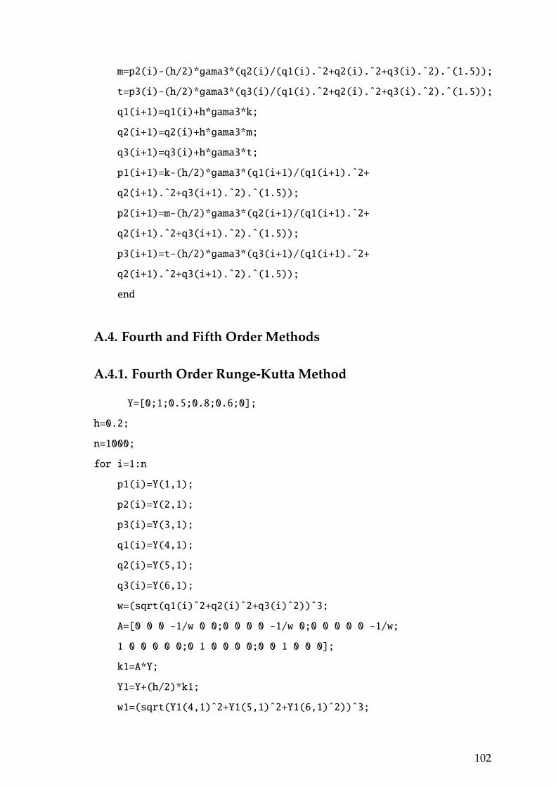
m=p2(i)-(h/2)*gama3*(q2(i)/(q1(i).ˆ2+q2(i).ˆ2+q3(i).ˆ2).ˆ(1.5));
t=p3(i)-(h/2)*gama3*(q3(i)/(q1(i).ˆ2+q2(i).ˆ2+q3(i).ˆ2).ˆ(1.5));
q1(i+1)=q1(i)+h*gama3*k;
q2(i+1)=q2(i)+h*gama3*m;
q3(i+1)=q3(i)+h*gama3*t;
p1(i+1)=k-(h/2)*gama3*(q1(i+1)/(q1(i+1).ˆ2+
q2(i+1).ˆ2+q3(i+1).ˆ2).ˆ(1.5));
p2(i+1)=m-(h/2)*gama3*(q2(i+1)/(q1(i+1).ˆ2+
q2(i+1).ˆ2+q3(i+1).ˆ2).ˆ(1.5));
p3(i+1)=t-(h/2)*gama3*(q3(i+1)/(q1(i+1).ˆ2+
q2(i+1).ˆ2+q3(i+1).ˆ2).ˆ(1.5));
end
A.4. Fourth and Fifth Order Methods
A.4.1. Fourth Order Runge-Kutta Method
Y=[0;1;0.5;0.8;0.6;0];
h=0.2;
n=1000;
for i=1:n
p1(i)=Y(1,1);
p2(i)=Y(2,1);
p3(i)=Y(3,1);
q1(i)=Y(4,1);
q2(i)=Y(5,1);
q3(i)=Y(6,1);
w=(sqrt(q1(i)ˆ2+q2(i)ˆ2+q3(i)ˆ2))ˆ3;
A=[0 0 0 -1/w 0 0;0 0 0 0 -1/w 0;0 0 0 0 0 -1/w;
1 0 0 0 0 0;0 1 0 0 0 0;0 0 1 0 0 0];
k1=A*Y;
Y1=Y+(h/2)*k1;
w1=(sqrt(Y1(4,1)ˆ2+Y1(5,1)ˆ2+Y1(6,1)ˆ2))ˆ3;
102

A1=[0 0 0 -1/w1 0 0;0 0 0 0 -1/w1 0;0 0 0 0 0 -1/w1;
1 0 0 0 0 0;0 1 0 0 0 0;0 0 1 0 0 0];
k2=A1*Y1;
Y2=Y+(h/2)*k2;
w2=(sqrt(Y2(4,1)ˆ2+Y2(5,1)ˆ2+Y2(6,1)ˆ2))ˆ3;
A2=[0 0 0 -1/w2 0 0;0 0 0 0 -1/w2 0;0 0 0 0 0 -1/w2;
1 0 0 0 0 0;0 1 0 0 0 0;0 0 1 0 0 0];
k3=A2*Y2;
Y3=Y+h*k3;
w3=(sqrt(Y3(4,1)ˆ2+Y3(5,1)ˆ2+Y3(6,1)ˆ2))ˆ3;
A3=[0 0 0 -1/w3 0 0;0 0 0 0 -1/w3 0;0 0 0 0 0 -1/w3;
1 0 0 0 0 0;0 1 0 0 0 0;0 0 1 0 0 0];
k4=A3*Y3;
Y=Y+(1/6)*h*(k1+2*k2+2*k3+k4);
L(i)=((q1(i)*p2(i)+q2(i)*p3(i)+q3(i)*p1(i))-
(q2(i)*p1(i)+q3(i)*p2(i)+q1(i)*p3(i)));
r(i)=abs(L(i)-L(1));
H(i)=0.5*((p1(i)).ˆ2+(p2(i)).ˆ2+(p3(i)).ˆ2)-1/
(sqrt((q1(i)).ˆ2+(q2(i)).ˆ2+(q3(i)).ˆ2));
e(i)=abs(H(i)-H(1));
H(1)=0.5*((p1(1)).ˆ2+(p2(1)).ˆ2+(p3(1)).ˆ2)-1/
(sqrt((q1(1)).ˆ2+(q2(1)).ˆ2+(q3(1)).ˆ2));
a=p1(1)*q1(1)+p2(1)*q2(1)+p3(1)*q3(1);
b=H(1)+(1/2)*sqrt((p1(1).ˆ2)+(p2(1).ˆ2)+(p3(1).ˆ2));
a1=(b*q1(1)-a*p1(1));
a2=(b*q2(1)-a*p2(1));
a3=(b*q3(1)-a*p3(1));
%Runge-Lenz vector
c=p1(i)*q1(i)+p2(i)*q2(i)+p3(i)*q3(i);
d=H(i)+(1/2)*sqrt((p1(i).ˆ2)+(p1(i).ˆ2)+(p1(i).ˆ2));
b1(i)=(d*q1(i)-c*p1(i));
b2(i)=(d*q2(i)-c*p2(i));
103

b3(i)=(d*q3(i)-c*p3(i));
R(i)=sqrt(((b1(i)-a1).ˆ2)+((b2(i)-a2).ˆ2)+((b3(i)-a3).ˆ2));
end
A.4.2. Composition Method of Order 5 (Midpoint as base method)
N = 1000;
h = 100/N ;
K = 1;
gama1=1/(4-(4ˆ(1/5)));
gama2=1/(4-(4ˆ(1/5)));
gama3=-((4ˆ(1/5))/(4-(4ˆ(1/5))));
gama4=1/(4-(4ˆ(1/5)));
gama5=1/(4-(4ˆ(1/5)));
%ilk deerler
q0 = [ 0.8 , 0.6 , 0 ]’ ;
p0 = [ 0 , 1 , 0.5 ]’ ;
r0 = sqrt( q0’*q0) ;
q1 = q0 ;
p1 = p0 ;
r1 = sqrt( q1’*q1) ;
%energy nin ilk deeri
H0 = ( ( p1’*p1/2 ) - ( K /r1 ) );
%angular momentum iin
m1 = q1(2)*p1(3) - q1(3)*p1(2);
m2 = q1(3)*p1(1) - q1(1)*p1(3);
m3 = q1(1)*p1(2) - q1(2)*p1(1);
%angular momentum un ilk deeri
104

L0 = [ m1 , m2 , m3 ]’ ;
%Runge-Lenz vector un ilk deeri
RL0 = q1 *(H0 + p1’*p1/2 ) - p1 *(q1’*p1) ;
% ----------------computational unit 1---------------
for i = 1:N
q11 = q1 ;
p11 = p1;
q21 = q11 ;
p21 = p11;
for k = 1:100
p_mid1 = (p1+p11)/2;
q21 = q1 + h *gama1* p_mid1 ;
q_mid1 = (q1+q11)/2;
r1 = sqrt( q_mid1’*q_mid1) ;
p21 = p1 - h*K*gama1*q_mid1/(r1ˆ3) ;
q11= q21;
p11 = p21;
end;
x1 = q11;
y1 = p11;
end;
105

%----------------computational unit 2------------------
q2 = x1 ;
p2 = y1 ;
r2 = sqrt( q2’*q2) ;
for i = 1:N
q12 = q2 ;
p12 = p2;
q22 = q12 ;
p22 = p12;
for k = 1:100
p_mid2 = (p2+p12)/2;
q22 = q2 + h *gama2* p_mid2 ;
q_mid2 = (q2+q12)/2;
r2 = sqrt( q_mid2’*q_mid2) ;
p22 = p2 - h*K*gama2*q_mid2/(r2ˆ3) ;
q12= q22;
p12 = p22;
end;
x2 = q12;
y2 = p12;
end;
106

%----------------computational unit 3------------------
q3 = x2 ;
p3 = y2 ;
r3 = sqrt( q3’*q3) ;
for i = 1:N
q13 = q3 ;
p13 = p3;
q23 = q13 ;
p23 = p13;
for k = 1:100
p_mid3 = (p3+p13)/2;
q23 = q3 + h *gama3* p_mid3 ;
q_mid3 = (q3+q13)/2;
r3 = sqrt( q_mid3’*q_mid3) ;
p23 = p3 - h*K*gama3*q_mid3/(r3ˆ3) ;
q13= q23;
p13 = p23;
end;
x3 = q13 ;
y3 = p13;
end;
107

%----------------computational unit 4------------------
q4 = x3 ;
p4 = y3 ;
r4 = sqrt( q4’*q4) ;
for i = 1:N
q14 = q4 ;
p14 = p4;
q24 = q14 ;
p24 = p14;
for k = 1:100
p_mid4 = (p4+p14)/2;
q24 = q4 + h *gama4* p_mid4 ;
q_mid4 = (q4+q14)/2;
r4 = sqrt( q_mid4’*q_mid4) ;
p24 = p4 - h*K*gama4*q_mid4/(r4ˆ3) ;
q14= q24;
p14 = p24;
end;
x4 = q14 ;
y4 = p14;
108

end;
%----------------computational unit 5------------------
q5 = x4 ;
p5 = y4 ;
r5 = sqrt( q5’*q5) ;
for i = 1:N
q15 = q5 ;
p15 = p5;
q25 = q15 ;
p25 = p15;
for k = 1:100
p_mid5 = (p5+p15)/2;
q25 = q5 + h *gama5* p_mid5 ;
q_mid5 = (q5+q15)/2;
r5 = sqrt( q_mid5’*q_mid5) ;
p25 = p5 - h*K*gama5*q_mid5/(r5ˆ3) ;
q15= q25;
p15 = p25;
end;
Q(:,i) = q15 ;
P(:,i) = p15;
T(i) = i*h ;
109

q5 = q15;
p5 = p15;
% energy
H(i) = ( ( p5’*p5/2 ) - ( K / sqrt(q5’*q5) ) ) ;
error_H(i) = H(i) - H0 ;
%angular momentum
mm1 = q5(2)*p5(3) - q5(3)*p5(2);
mm2 = q5(3)*p5(1) - q5(1)*p5(3);
mm3 = q5(1)*p5(2) - q5(2)*p5(1);
L(:,i) = [mm1 , mm2 , mm3 ]’ ;
error_L(:,i) = sqrt( (L(:,i) - L0)’*(L(:,i)-L0)) ;
%runge-lenz vector
RL(:, i) = q5 *(H(i) + p5’*p5/2 ) - p5 *(q5’*p5) ;
error_RL(:,i) = sqrt( (RL(:,i)- RL0)’*(RL(:,i)- RL0)) ;
end;
A.4.3. Composition Method of Order 5 (Stormer-Verlet as base
method)
q11(1)=0.8;
q21(1)=0.6;
p11(1)=0;
p21(1)=1;
q31(1)=0;
p31(1)=0.5;
110

%h=0.01;
gama1=1/(4-(4ˆ(1/5)));
gama2=1/(4-(4ˆ(1/5)));
gama4=1/(4-(4ˆ(1/5)));
gama5=1/(4-(4ˆ(1/5)));h=0.08;
gama3=-((4ˆ(1/5))/(4-(4ˆ(1/5))));
% for s=1:8;
% h=(1/5)ˆs;
% x(s)=h;
for i=1:1000;
k=p11(i)-(h/2)*gama1*(q11(i)/(q11(i).ˆ2+q21(i).ˆ2+
q31(i).ˆ2).ˆ(1.5));
m=p21(i)-(h/2)*gama1*(q21(i)/(q11(i).ˆ2+
q21(i).ˆ2+q31(i).ˆ2).ˆ(1.5));
t=p31(i)-(h/2)*gama1*(q31(i)/(q11(i).ˆ2+
q21(i).ˆ2+q31(i).ˆ2).ˆ(1.5));
q11(i+1)=q11(i)+h*gama1*k;
q21(i+1)=q21(i)+h*gama1*m;
q31(i+1)=q31(i)+h*gama1*t;
p11(i+1)=k-(h/2)*gama1*(q11(i+1)/(q11(i+1).ˆ2+
q21(i+1).ˆ2+q31(i+1).ˆ2).ˆ(1.5));
p21(i+1)=m-(h/2)*gama1*(q21(i+1)/(q11(i+1).ˆ2+
q21(i+1).ˆ2+q31(i+1).ˆ2).ˆ(1.5));
p31(i+1)=t-(h/2)*gama1*(q31(i+1)/(q11(i+1).ˆ2+
q21(i+1).ˆ2+q31(i+1).ˆ2).ˆ(1.5));
end
p12(1)=p11(1001);
p22(1)=p21(1001);
q12(1)=q11(1001);
111

q22(1)=q21(1001);
p32(1)=p31(1001);
q32(1)=q31(1001);
for i=1:1000;
k=p12(i)-(h/2)*gama2*(q12(i)/(q11(i).ˆ2+q22(i).ˆ2+
q32(i).ˆ2).ˆ(1.5));
m=p22(i)-(h/2)*gama2*(q22(i)/(q12(i).ˆ2+q22(i).ˆ2+
q32(i).ˆ2).ˆ(1.5));
t=p32(i)-(h/2)*gama2*(q32(i)/(q12(i).ˆ2+q22(i).ˆ2+
q32(i).ˆ2).ˆ(1.5));
q12(i+1)=q12(i)+h*gama2*k;
q22(i+1)=q22(i)+h*gama2*m;
q32(i+1)=q32(i)+h*gama2*t;
p12(i+1)=k-(h/2)*gama2*(q12(i+1)/(q12(i+1).ˆ2+
q22(i+1).ˆ2+q32(i+1).ˆ2).ˆ(1.5));
p22(i+1)=m-(h/2)*gama2*(q12(i+1)/(q12(i+1).ˆ2+
q22(i+1).ˆ2+q32(i+1).ˆ2).ˆ(1.5));
p32(i+1)=t-(h/2)*gama2*(q32(i+1)/(q12(i+1).ˆ2+
q22(i+1).ˆ2+q32(i+1).ˆ2).ˆ(1.5));
end
p13(1)=p12(1001);
p23(1)=p22(1001);
q13(1)=q12(1001);
q23(1)=q22(1001);
p33(1)=p32(1001);
q33(1)=q32(1001);
for i=1:1000;
k=p13(i)-(h/2)*gama3*(q13(i)/(q13(i).ˆ2+q23(i).ˆ2+
q33(i).ˆ2).ˆ(1.5));
m=p23(i)-(h/2)*gama3*(q23(i)/(q13(i).ˆ2+q23(i).ˆ2+
112

q33(i).ˆ2).ˆ(1.5));
t=p33(i)-(h/2)*gama3*(q33(i)/(q13(i).ˆ2+q23(i).ˆ2+
q33(i).ˆ2).ˆ(1.5));
q13(i+1)=q13(i)+h*gama3*k;
q23(i+1)=q23(i)+h*gama3*m;
q33(i+1)=q33(i)+h*gama3*t;
p13(i+1)=k-(h/2)*gama3*(q13(i+1)/(q13(i+1).ˆ2+
q23(i+1).ˆ2+q33(i+1).ˆ2).ˆ(1.5));
p23(i+1)=m-(h/2)*gama3*(q13(i+1)/(q13(i+1).ˆ2+
q23(i+1).ˆ2+q33(i+1).ˆ2).ˆ(1.5));
p33(i+1)=t-(h/2)*gama3*(q33(i+1)/(q13(i+1).ˆ2+
q23(i+1).ˆ2+q33(i+1).ˆ2).ˆ(1.5));
end
p14(1)=p13(1001);
p24(1)=p23(1001);
q14(1)=q13(1001);
q24(1)=q23(1001);
p34(1)=p33(1001);
q34(1)=q33(1001);
for i=1:1000;
k=p14(i)-(h/2)*gama4*(q14(i)/(q14(i).ˆ2+q24(i).ˆ2+
q34(i).ˆ2).ˆ(1.5));
m=p24(i)-(h/2)*gama4*(q24(i)/(q14(i).ˆ2+q24(i).ˆ2+
q34(i).ˆ2).ˆ(1.5));
t=p34(i)-(h/2)*gama4*(q34(i)/(q14(i).ˆ2+q24(i).ˆ2+
q34(i).ˆ2).ˆ(1.5));
q14(i+1)=q14(i)+h*gama4*k;
q24(i+1)=q24(i)+h*gama4*m;
q34(i+1)=q34(i)+h*gama4*t;
p14(i+1)=k-(h/2)*gama4*(q14(i+1)/(q14(i+1).ˆ2+
q24(i+1).ˆ2+q34(i+1).ˆ2).ˆ(1.5));
113

p24(i+1)=m-(h/2)*gama4*(q14(i+1)/(q14(i+1).ˆ2+
q24(i+1).ˆ2+q34(i+1).ˆ2).ˆ(1.5));
p34(i+1)=t-(h/2)*gama4*(q34(i+1)/(q14(i+1).ˆ2+
q24(i+1).ˆ2+q34(i+1).ˆ2).ˆ(1.5));
end
p1(1)=p14(1001);
p2(1)=p24(1001);
q1(1)=q14(1001);
q2(1)=q24(1001);
p3(1)=p34(1001);
q3(1)=q34(1001);
H(1)=0.5*((p1(1)).ˆ2+(p2(1)).ˆ2+(p3(1)).ˆ2)-1/
(sqrt((q1(1)).ˆ2+(q2(1)).ˆ2+(q3(1)).ˆ2));
a=p1(1)*q1(1)+p2(1)*q2(1)+p3(1)*q3(1);
b=H(1)+(1/2)*sqrt((p1(1).ˆ2)+(p2(1).ˆ2)+(p3(1).ˆ2));
a1=(b*q1(1)-a*p1(1));
a2=(b*q2(1)-a*p2(1));
a3=(b*q3(1)-a*p3(1));
for i=1:1000;
% Energy
H(i)=0.5*((p1(i)).ˆ2+(p2(i)).ˆ2+(p3(i)).ˆ2)-1/
(sqrt((q1(i)).ˆ2+(q2(i)).ˆ2+(q3(i)).ˆ2));
e(i)=abs(H(i)-H(1));
%angular momentum
L(i)=((q1(i)*p2(i)+q2(i)*p3(i)+q3(i)*p1(i))-
(q2(i)*p1(i)+q3(i)*p2(i)+q1(i)*p3(i)));
r(i)=abs(L(i)-L(1));
%Runge-Lenz vector
c=p1(i)*q1(i)+p2(i)*q2(i)+p3(i)*q3(i);
114
d=H(i)+(1/2)*sqrt((p1(i).ˆ2)+(p1(i).ˆ2)+(p1(i).ˆ2));
b1(i)=(d*q1(i)-c*p1(i));
b2(i)=(d*q2(i)-c*p2(i));
b3(i)=(d*q3(i)-c*p3(i));
R(i)=sqrt(((b1(i)-a1).ˆ2)+((b2(i)-a2).ˆ2)+((b3(i)-a3).ˆ2));
k=p1(i)-(h/2)*gama5*(q1(i)/(q1(i).ˆ2+q2(i).ˆ2+q3(i).ˆ2).ˆ(1.5));
m=p2(i)-(h/2)*gama5*(q2(i)/(q1(i).ˆ2+q2(i).ˆ2+q3(i).ˆ2).ˆ(1.5));
t=p3(i)-(h/2)*gama5*(q3(i)/(q1(i).ˆ2+q2(i).ˆ2+q3(i).ˆ2).ˆ(1.5));
q1(i+1)=q1(i)+h*gama5*k;
q2(i+1)=q2(i)+h*gama5*m;
q3(i+1)=q3(i)+h*gama5*t;
p1(i+1)=k-(h/2)*gama5*(q1(i+1)/(q1(i+1).ˆ2+q2(i+1).ˆ2+
q3(i+1).ˆ2).ˆ(1.5));
p2(i+1)=m-(h/2)*gama5*(q2(i+1)/(q1(i+1).ˆ2+q2(i+1).ˆ2+
q3(i+1).ˆ2).ˆ(1.5));
p3(i+1)=t-(h/2)*gama5*(q3(i+1)/(q1(i+1).ˆ2+q2(i+1).ˆ2+
q3(i+1).ˆ2).ˆ(1.5));
end
115