Comparison of experimental and numerical sloshing loads in partially filled tanks

S. Brizzolara, L. Savio & M. Viviani

Y. Chen & P. Temarel

N. Couty & S. Hoflack

L. Diebold & N. Moirod

A. Souto Iglesias

ABSTRACT: Sloshing phenomenon consists in the movement of liquids inside partially filled tanks, which generates dynamic loads on the tank structure. Resulting impact pressures are of great importance in assessing structural strength, and their correct evaluation still represents a challenge for the designer due to the high nonlinearities involved, with complex free surface deformations, violent impact phenomena and influence of air trapping. In the present paper a set of two-dimensional cases for which experimental results are available are considered to assess merits and shortcomings of different numerical methods for sloshing evaluation, namely two commercial RANS solvers (FLOW-3D and LS-DYNA), and two own developed methods (Smoothed Particle Hydrodynamics and RANS). Impact pressures at different critical locations and global moment induced by water motion for a partially filled tank with rectangular section having a rolling motion have been evaluated and results are compared with experiments.

1 INTRODUCTION

The sloshing phenomenon is a highly nonlinear movement of liquids inside partially filled tanks with oscillatory motions. This liquid movement gener­ates dynamic loads on the tank structure and thus becomes a problem of relative importance in the design of marine structures in general and an espe­cially important problem in some particular cases (Tveitnes et al. 2004).

In some cases, this water movement is used for dampening ship motions (passive anti-roll tanks), especially for vessels with low service speed (fish­ing vessels, supply vessels, oceanographic and re­search ships, etc.) and for which active fin stabilizers would not produce a significant effect (Lloyd 1989).

The sloshing problem has been to a great extent investigated in the last 50 years, with increasing levels of accuracy and computational efforts.

First attempts were based on mechanical models of the phenomenon by adjusting terms in the har­monic equation of motion (Graham & Rodriguez 1952, Lewison 1976). These types of techniques are used when time-efficient and not very accurate results are needed (Aliabadi et al. 2003).

The second series of investigations solves a poten­tial flow problem with a very sophisticated treatment of the free-surface boundary conditions (Faltinsen et al. 2005) that extends the classical linear wave theory by performing a multimodal analysis of the free-surface behavior. This approach is very time efficient and accurate for specific applications but it does not allow to model overturning waves and may present problems when generic geometries and/or baffled tanks are considered.

The third group of methods solves the nonlinear shallow water equations (Stoker 1957) with the use of different techniques (Lee et al. 2002, Verhagen & Van Wijngaarden 1965).

The fourth group of techniques used to deal with highly nonlinear free-surface problems is aimed at solving numerically the incompressible Navier—Stokes equations. Frandsen (2004) solves the nonlinear poten­tial flow problem with a finite difference method in a 2-D tank that is subjected to horizontal and verti­cal motion, with very good results, but this approach suffers from similar shortcomings to the multimodal method. Celebi and Akyildiz (2002) solve the com­plete problem by using a finite difference scheme and a VOF formulation for tracking the free-surface. Sames et al. (2002) present results carried out with a commercial finite volume VOF method applied to both rectangular and cylindrical tanks. Schellin et al. (2007) present coupled ship/sloshing motions with very promising results.

In general, numerical techniques present signif­icant problems when considering highly nonlinear waves and/or overturning waves, the effect of air cushions and fluid-structure interactions. Considering the first problem, Smoothed Particle Hydrodynam­ics (SPH) meshless method appears as a promising alternative to standard grid based techniques because of their intrinsic capability to capture surface defor­mations. Literature about SPH applications to typical marine problems is not very abundant; in Colagrossi et al. 2003 one of the first applications is shown. In successive years, a certain number of applications devoted to the assessment of slamming phenomenon (Oger et al. 2006, Viviani et al. 2007a, b 2008) are found. Sloshing phenomenon is considered by Souto Iglesias et al. 2006 and Delorme et al. 2008b, in which a comprehensive series of calculations is performed focusing attention on resulting global moment and its dependence with tank oscillating frequency, but prob­lems related to the evaluation of local impact pressures are still considerable, with presence of significantly oscillating results.

The activity described in the present paper, which was carried out in the framework of the EU funded MARSTRUCT Network of Excellence, covered three two-dimensional (or infinite length) cases, focusing on impact pressures and global moments into a par­tially filled tank with rectangular section, which has an oscillatory rolling motion with different periods and different water levels. For these tests, experimental measurements were carried out by the Model Basin Research Group (CEHINAV) of the Naval Architecutre Department (ETSIN) of the Technical University of Madrid (UPM), in the context of a comprehensive analysis of sloshing phenomenon, as reported by Delorme et al. (2007 and 2008a).

A series of numerical techniques has been applied by various participants to assess their merits and short­comings, and in particular:

- a RANS code own-developed by UoS (University of Southampton)

- two available commercial software for the solution of RANS equations, namely FLOW-3D applied by BV (Bureau Veritas) and LS-DYNA applied by PRI (Principia)

- a SPH code own developed by DINAV (University of Genoa).

2 EXPERIMENTAL SET-UP

The experimental tests which are used for benchmark­ing the various numerical techniques were performed by CEHINAVETSIN-UPM, as reported in Delorme et al. 2007 and 2008a.

In particular, a rectangular tank having dimensions (in centimeters) reported in Fig. 1 was considered. The tank is cylindrical, and the dimension perpendicular to those reported in Fig. 1 is 62 mm; a sinusoidal rolling motion has been imposed during experiments, with a rolling axis located 18.4 cm over the bottom line, an amplitude of 4° in all cases and different periods.

The tank was fitted for a series of sensors in dif­ferent locations, as indicated in Fig. 1. During exper­iments, pressures in correspondence to the two most critical positions were recorded. The sensors are BTE6000—Flush Mount, with a 500 mbar range.

In parallel to pressure measurements, global torque measurement were conducted. In particular, torque time history was measured during experiments with water inside the tank and with empty tank, then the first harmonic of the moment response of the liquid with respect to the tank rotating centre for every case was obtained postprocessing data.

In table 1, the two water levels considered in present analysis are reported, together with the correspondent natural period of oscillation.

_M

'

• 14 .«

1

I

8 S

Figure 1. Tank geometry and position of the sensors.

Table 1. Water levels considered.

Level Level/ Natural symbol Level [cm] tank height Period To [s]

9.3 22.2

18.3% 43.7%

1.91 1.32

Table 2 Test Cases description.

Case Level/tank height Period [s] Period/To

1 A—18.3% 1.91 1.0 2 B ^ B . 7 % 1.19 0.9 3 B ^ B . 7 % 1.32 1.0

500

0

Case A - T = T0 - Sensor 1

-r 4 -f

i—Ji-F""1 T — ft"" -1-

Case B - T = 0.9T - Sensor 6

15 20 25 3C

Figure 2. Sensor 1.

Test Case 1—Level A—T = To—Pressure at

For both water levels, experiments carried out in correspondence to the resonance period have been considered (case 1 and 3 for level A and B respec­tively), to have large free surface deformation and analyse codes' capability to capture it. Moreover, for case B a lower oscillating period (90% of the reso­nance one) has been analysed (case 2), in which a marked beating phenomenon has been observed.

In table 2, main characteristics of cases analysed are briefly summarized for a better understanding.

In correspondence to case 1, pressure sensors are located at positions 1 and 6, and impacts were recorded on sides in correspondence to lower sensor, as pre­sented in following Fig. 2.

In correspondence to cases 2 and 3, pressure sen­sors were located at positions 3 and 6; as anticipated, case 2 is interesting for the presence of beating type kinematics and pressures, with peak values oscillat­ing, as presented in following Fig. 3 for sensor 6. Regarding case 3, pressure peaks were recorded in correspondence to both locations as reported in Fig. 4, with impact events at the tank top (sensor 3) and pres­sure rises due to the incoming wave and to water fall after impact at sensor 6.

In addition to pressure measurement, in follow­ing table 3 the resulting first harmonic of the liquid moment is reported.

In particular, Mo is the first harmonic amplitude and <f> is the phase lag with respect to oscillating motion, resulting in equation (1) for time history, considering the motion period T:

/2TT M = M0 sin ( — t

TÍT 1

TIII • mini ilium m i n i 11111111 mini mini iimri"iH|"rn

1 Ml H H • , I 1 1 1 1 1 fl fl i i A i 11

"WM\—M I - ¡i I IHHHHfHHr MHf \\i fttt ••.iiiiiiiiiiiriiiin IIIIIIIIIIIIIIIIIIIIIIIIIIIII L»ij,»iPii'i"ii"i"i |ii«i['i"ii»i"i l ,ir ,i"i"i"i"i"i"ii"i l:i"i 15 20 25 30 35

Figure 3. Test Case 2—Level B—T = 0.9 To—Pressure at Sensor 6.

Case B - T=T. - Sensors 3 and 6

1SJ_*J

— d — _| —

_k2|*,l_ki_¿IiA,(jJ_i,LLkJ_kJi_ík¿:

= E

» i L l U

Figure 4. Test Case 3—Level B—T = To—Pressure at Sensors 3-6.

Table 3.

Case

1 2 3

Oscillating

M0[Nm]

4.52 1.07 6.70

moment first harmonic values.

Mo[Nm/m]

72.87 17.22

108.03

<t> [deg]

84.4 173.6 112.0

(1)

First harmonic Mo value is reported both for the real experimental case (tank with 62 mm third dimension) and for the equivalent two-dimensional configuration, for which moment per unit length is given.

Rolling motion during experiments was a pure sinu­soidal motion apart at the very beginning of the exper­iment to avoid infinite accelerations.

Finally, a proper uncertainty analysis has not been conducted yet since it is hard to find a consistent approach to it in this case. This is due to the strong chaotic character of the pressure peaks, as discussed in Delorme et al. 2008, where the initial steps to such analysis were given.

3 DESCRIPTION OF METHODS

Methods used for modeling the sloshing phenomenon are summarized in Tables 4 and 5 for test case 1 and

Lable 4. Details of method and idealization—Lest case 1. Lable 6. Outline of sloshing cases.

Participant

UoS DINAV

PRI BV

Method

RANS SPH

LS-DYNA FLOW 3D

Idealisation details

55 x 50 grid 37138 real particles

1876 virtual particles 90 x 51 grid 5 x 220 x 122 grid

Case

Case 1 Case 2 Case 3

£

1.5 * Az 1.5 * Az 1.5 * Az

Lime step [s]

1.0 x 10~3

1.0 x 10~3

1.0 x 10~3

Lable 5. Details of method and idealization—Lest case 2-3.

Participant Method Idealisation details

UoS DINAV

PRI BV

RANS SPH

LS-DYNA FLOW 3D

90 x 50 grid 88652 real particles

1876 virtual particles 90 x 51 grid 5 x 90 x 62 grid

for test cases 2 and 3, respectively; in the same tables, some details of the idealization are also included.

In SPH real particles are used to represent water, while virtual ones are used to represent the moving tank. For both of them a diameter of 1.5 mm has been adopted. BV calculations are 3-dimensional, and the experimental setup was effectively reproduced, while in all other cases a two-dimensional problem was ana­lyzed. Only UoS considered air (and pressure vari­ations inside it), while in all other cases only water was considered (in VoF methods, air is schematized as void). Finally, effective time histories were applied both by BV (case 1 only) and PRI, while pure har­monic oscillations were applied by BV (case 2 and 3), UoS and DINAV; it resulted from calculations that this has not a significant impact once phenomena are stabilized.

3.1 RANS approach adopted by UoS

Lhe level set formulation in a generalized curvilinear coordinates system has been developed to simulate the free surface waves generated by moving bodies or sloshing of fluid in a container. The Reynolds-averaged Navier-Stokes (RANS) equations are mod­ified to account for variable density and viscosity for the two-fluid flows (i.e. water-air). By computing the flow fields in both the water and air regions, the location and transport of free surface inside a tank is automatically captured. A detailed description of the numerical method can be found in Chen et al. 2008.

In the simulation of sloshing, appropriate boundary conditions need to be imposed to calculate the impact loads. Traditionally, in a single phase flow solver, a thin artificial buffer zone is adopted near the tank ceil­ing and a linear combination of free surface and rigid

wall conditions imposed inside the buffer zone. The magnitude of the impact pressure is affected by several factors such as the choice of time step and thickness of the buffer zone, as discussed in Chen et al. 2008. In the present investigation there is no special treatment required for the free surface as a two-fluid approach is used to solve the RANS equations in both water and air regions in a unified manner and the interface is only treated as a shift in fluid properties. The solid wall boundary condition is imposed by vanishing the normal velocity to the wall or setting the components of velocity on the wall to zero. The wall pressure is obtained by projecting the momentum equation along the normal to the wall.

In addition to data already provided in previous paragraph, other computational conditions are listed in Table 6, indicating the values of half the finite thick­ness of the interface in which density and viscosity change and time step increment examined in this study (Az represents the vertical distance between two grid nodes and e the interface half thickness).

Regarding torque calculations, for this method they are provided for case 1 only since some problems have been encountered for other cases, which are still under investigation.

3.2 LS-DYNA approach adopted by PRI

The LS-DYNA software is used. This is an explicit finite element code solving the mechanics equations (here corresponding more precisely to the RANSE with Reynolds stresses neglected). The fluid domain is modelled using a multi-materials Eulerian for­mulation. For the advection of the variables at the integration points, a Van Leer scheme (second order precision) is used and a Half Index Shift (HIS) method for the nodal variables. Each material is character­ized by a volume fraction inside each element. It interacts in the calculation of the "composite" pres­sure for the partially filled cells within a Volume Of Fluid (VOF) method. The dispersion of the volume fraction for these particular cells is limited with an interface reconstruction method (boundary between materials modelled as a plane). Air is modeled as void.

The problem is addressed in two dimensions, although under-integrated 8-noded elements (one layer in the direction normal to the plane) are used

Figure 5. Eulerian mesh for case 1 (water in red, void in blue).

to model the fluid domain in practice. The size of the fluid cells is of 10 mm edge length, chosen close to the sensor size. The mesh, using 90 x 51 solid elements, can be seen in Fig. 5 for cases 1. Cases 2 and 3 are schematized in the same way, except that level of water is modified in accordance to test setup.

The behaviour of water is modelled with a polyno­mial equation of state, and no viscosity is defined.

The fluid domain is surrounded with one layer of rigid elements (in grey on Fig. 5), modeling the wall and preventing normal flow. Besides, the movement (as given by the roll time histories) is imposed to this rigid part, then the rigid movement of the Eulerian grid (following the walls) is achieved by forcing the grid to follow the movement of three nodes of the rigid part (Aquelet et al. 2003).

The time scheme is based on the Finite Difference method, which is conditionally stable. Thus, the time step is linked to the shortest duration for an acoustic wave to cross any element of the model (fluid or solid), close to 6 |xs here.

Pressure histories are directly post-treated in solid elements where sensors are located.

3.3 Smoothed particle hydrodynamics method, adopted by DINAV

SPH is a Lagrangian meshless CFD method, initially developed for compressible fluids (Gingold and Mon-aghan 1977) and successively adapted and corrected for hydrodynamic problems (Liu and Liu, 2003). The continuum is discretized in a number of particles, each representing a certain finite volume of fluid, which are followed in a Lagrangian way during their motions induced by internal forces between nearby interacting particles and external mass forces or boundary forces. Internal forces derive from the usual Navier-Stokes and continuity equations, made discrete in space by means of a kernel formulation. In general, if A is a field variable and W is the kernel function, the

following equations (already in their discretised form) are adopted:

N

(A(r)) = ^2 — A(-rj) w(r ~ ri>h) (2) 7 = 1 Pj

where my and p¡ are mass and density of the y'th particle, r and r¡ are position vectors in space and for the y'th particle, respectively. The term h represents the smoothing length, which determines the extent to which a certain particle has influence on the others. Different kernel functions may be utilized (Liu and Liu 2003); in particular, in the present work, Gaussian kernel was adopted. The resulting formulae, in the particles approximation, for the continuity equation and the momentum equation are:

dpi/dt = J2 mjivi -vj)- VW(r - r¡, h),

dvjdt = -Y^mjipjpf +Pj/pf)VW(r - rj,h) +g

(3)

Moreover, in order to close the problem, an equa­tion of state (Monaghan 1994) which relates density to pressure for each particle, considering the fluid as "weakly compressible", is adopted:

p=áfl\(£-Y-A (4) y l\poJ

where po is reference density (1000 kg/m3) and p is density of each particle. Constant y is set to 7 in accordance to Batchelor 1967, providing satisfac­tory results for various SPH applications. The value of sound speed Co cannot, in general, be set to its effective value for practical reasons (i.e. time steps become too small); thus, it is usually set in order to limit the Mach number to a value below 0.1 (Mon­aghan 1994) and, consequently, density variations in the incompressible flow to acceptable values. In par­ticular, in accordance to previous works (Viviani et al. 2008), sound speed was set in order to limit density variations to values below 1%; for all cases consid­ered, a value of 50 m/s was sufficient to achieve this condition; according to this, a time step of 10~5 s was adopted, which is about half the one required by the simple application of Courant condition (according to previous experience).

Since SPH can be affected by a lack of stability, various authors developed different methods which can help in reducing this problem, such as Artificial Viscosity and XSPH (Monaghan 1992); in present calculations, on the basis of previous experiences (Viviani et al. 2007a, b), it was decided to avoid XSPH, and to consider an artificial viscosity term as reported in equations (5) where c, p, and h are sound

speed, density, smoothing length and kernel function respectively and the subscript 'ij' represents a mean value.

n„ -BlCij<t>ij + ,

Pi) Vij • Xij < 0

Vy • Xjj > 0

(5)

"y '^y ' Xij

\xij\ +(ehij)

A comprehensive analysis was carried out to obtain the best setup of parameters a, fi and e (results can­not be included for space limitations), and after it they were all set to the low value of 0.01, thus almost neglecting also artificial viscosity.

With reference to boundary treatment, repulsive forces are used as suggested by Monaghan (1994), adopting a force which is dependent on the inverse of the distance between fluid and boundary particles according to the formulation of Lennard-Jones for molecular force, as described by Equation (6), where pi = 12 and p2 = 6, ro is the cutting-off distance, approximately equal to the smoothing length, and r is distance between real and boundary particles:

f(r) = 0, elsewhere

when r < ro

(6)

Finally, in order to evaluate pressure an approach similar to the one presented by Oger et al. (2006) was adopted, albeit simplified since pressure is evaluated as a mean of values computed for real particles in proximity of the boundary particle, i.e. in a rectan­gular region with width parallel to boundary surface and height perpendicular to boundary surface which are multiples of the smoothing length (in particular, a 4 x 1 0 region was considered).

3.4 FlowSD approach, adopted by BV

FLOW-3D solves the transient Navier-Stokes equa­tions by a finite volume/finite differences method in a fixed Eulerian rectangular grid. One of its distinc­tive features is the Fractional Area Volume Obstacle Representation (FAVOR) technique, which allows for the definition of solid boundaries within the Eulerian grid. Using such a technique definition of boundaries and obstacles is carried out independent of the grid generation.

In particular, the 1 -phase flow option was used for this calculation; regarding time, the real time roll series was used as input motion for Case A, while for case B (both T = 0.9To and T = To), harmonic excitations were adopted for the sake of simplicity, since it was

found that differences were not important. Finally the x-direction was also considered, with a "depth" equal to 6.2 cm, as utilized also in the experiments.

4 RESULTS AND DISCUSSION

4.1 Test case 1—Water Level A—T = To

In general, this is the case for which the most com­prehensive analysis was carried out. In particular, a rather large number of computations was performed with SPH to analyse the effect of some parameters, and in particular of time step and of artificial viscos­ity; results of this analysis are not included in present paper for space limitations, and only final setup results are presented (time step equal to 10~5 s, XSPH and artificial viscosity parameters set to 0.01). It has to be mentioned, however, that influence of artificial vis­cosity is very pronounced, and in particular higher val­ues result in an overdamping of all phenomena (with impact pressures almost vanishing in correspondence to values of a and fi in artificial viscosity equal to 0.3), without overturning waves, and with lower pressure peaks.

In Figs. 6 and 7, pressure at Sensor 1 results obtained with all methods are summarized (Fig. 6 represents results obtained in the first part of the simulation/experiment, while Fig. 7 represents a larger

e A - T=T - Sensor 1

e A - T=T„ - Sensor 1

m k m Figure 6. Test Case 1—Level A—T = To—Sensor 1 pres­sure time history—first two oscillations (upper) and up to t = 10s (lower).

Case A - T=T0 - Sensor 1

2'500 • i i i i • i i i i • i i i i • i i i i • i • i i i i •

2'000

10 12 14 16 18 20 22 24 26 28 80

tlsl

Figure 7. Test Case 1—Level A—T = To—Sensor 1 pressure time history for t = 10-30 s.

scale); in general, pressure peak order of magnitude is captured by all methods applied.

For all of them, first peak is captured correctly (con­sidering mean values in the whole time history), and the second peak is also captured, even if its amplitude accuracy is not as good as the one of the first peak. SPH calculations provide a higher peak at fourth oscil­lation, similarto some values obtained by PRI at longer time, while UoS results provide a peak which has the correct order of magnitude but a narrower form.

Looking at Fig. 7 for longer times (only BV and PRI calculations have been extended to that), both methods still provide accurate results, even if BV cal­culations are probably more robust (with lower oscil­lations) and similarto experimental ones. Calculations with SPH were not extended to these higher times because of long calculation times, and attention was paid to calibration of various parameters as explained before. Once a satisfactory setup was obtained, this was applied to other cases to better analyze its general nature.

In following Fig. 8 results obtained for sensor 6 are reported. In this case, pressure values are lower by an order of magnitude with respect to those encountered for previous Sensor 1, representing more a "sensor wetting" (thus a less critical point) rather than a real impact phenomenon.

Keeping this in mind, only BV and UoS meth­ods are able to reproduce the experimental pressure peaks, while SPH overestimates them and provides in some cases anomalous negative values (which are present also for UoS); in all cases a time history differ­ent from the experimental one is produced, with faster pressure decay than recorded.

PRI method seems only to be capable of signaling the "senor wetting" occurrences after the first 10 sec­onds of calculations, with the presence of a repetitive phenomenon with the same period of the experimental one, however pressure peaks seem to be most of time overestimated, and anomalous negative values result.

In following Fig. 9, results in terms of global torque, as evaluated by DINAV UoS and PRI are reported.

CaseA-T=TD -Sensor6

SPH Experimental Po\NSE_BV Po\NSE_PRI Po\NSE_UoS

Figure 8. Test Case 1—Level A—T = To—Sensor 6 pressure time history up to t = 30 s.

CaseA-T=T0 Torque

t[s]

Figure 9. Test Case 1—Level A—T = To—Global torque time history up to t = 25 s.

Only results after the first period are reported, in order to look at the " stabilized values" cutting the ini­tial transient phase; this allows a better comparison with experimental results which, as already under­lined, are referred only to the first harmonic of oscil­lating torque time history.

Regarding SPH calculations, results reported are referred as before to the best setup from preliminary analysis. It has to be noticed, however, that once global torque is considered instead of local pressure, dif­ferences between various setups are reduced, with the presence of similar results for a wide range of settings of artificial viscosity terms. This result is due to the fact that pressure integration needed to obtain the resultant torque acts like a low-pass fil­ter, smoothing pressure oscillations and cutting the effect of localized pressure peaks. Differences can still be found in correspondence to torque peaks, with values obtained in correspondence to the lowest a and fi values in artificial viscosity which are about 10-15% higher than the correspondent ones obtained with high a and fi.

I

Figure 10-11. Kinematics capturing with SPH—overturn­ing wave (upper) and flow rise after impact (lower).

Figure 12-13. Kinematics capturing with LS-DYNA— overturning wave (upper) and flow rise after impact (lower).

Comparing results to experiments, SPH tends to underestimate by about 10% the effective oscillating torque amplitude. PRI results are more consistent with experiments, even if in the central part of the simula­tion they present an anomalous behavior, with a sort of beating phenomenon. UoS results are probably the best with a lower mean error and a higher stability, even if they are limited to the first 10 seconds.

Figure 14—15. Kinematics during experiments-ing wave at two successive periods.

Finally, in following figures some examples of kine­matic capturing are presented (10-11 for SPH, 12-13 for LS-DYNA, 14-15 for experiments), showing a good qualitative capturing of sloshing impact phenom­ena and of overturning waves.

4.2 Test case 2—Water Level B—T = 0.9 T0

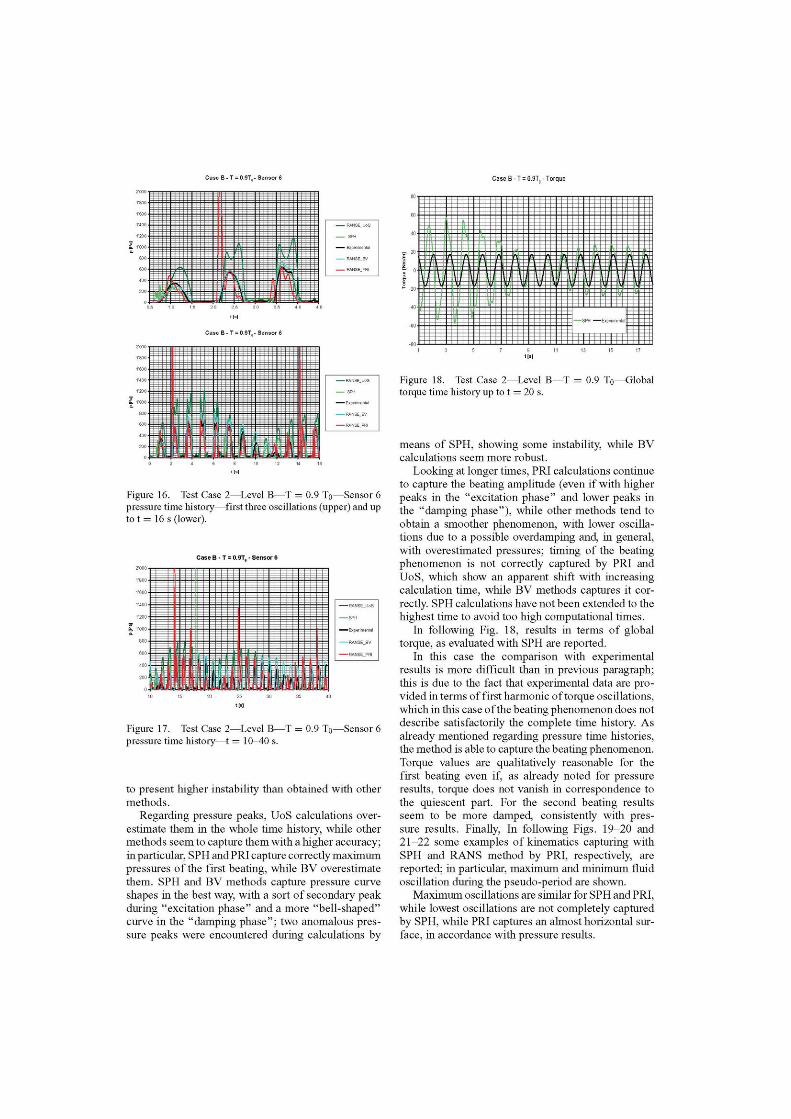
In Figs. 16-17, results obtained with all methods for Sensor 6 are summarized; as already mentioned, this case is considerably different from the others, since strong impacts are not expected, but just flow oscilla­tions; interest in this case is due to the presence of a beating type phenomena, with pressure peaks of oscil­lating amplitude and not periodic with the same value for each period.

For all methods applied the beating phenomenon is captured qualitatively, even if most of the numerical codes do not allow to simulate the almost complete quiescence of fluid with pressures near to zero. Only PRI calculations allow obtaining the low pressures in correspondence to the beating, even if they seem

-T = 0.9T„-Sensor6 Case B - T = 0.9T -Torque

-T = 0.9T„-Sensor6

Figure 16. Test Case 2—Level B—T = 0.9 To—Sensor 6 pressure time history—first three oscillations (upper) and up to t = 16 s (lower).

Case B - T = 0.9Tn - Sensor 6

Figure 17. Test Case 2—Level B—T = 0.9 To—Sensor 6 pressure time history—t = 10-40 s.

to present higher instability than obtained with other methods.

Regarding pressure peaks, UoS calculations over­estimate them in the whole time history, while other methods seem to capture them with a higher accuracy: in particular, SPH and PRI capture correctly maximum pressures of the first beating, while BV overestimate them. SPH and BV methods capture pressure curve shapes in the best way, with a sort of secondary peak during "excitation phase" and a more "bell-shaped" curve in the "damping phase"; two anomalous pres­sure peaks were encountered during calculations by

Figure 18. Test Case 2—Level B—T = 0.9 T0—Global torque time history up to t = 20 s.

means of SPH, showing some instability, while BV calculations seem more robust.

Looking at longer times, PRI calculations continue to capture the beating amplitude (even if with higher peaks in the "excitation phase" and lower peaks in the "damping phase"), while other methods tend to obtain a smoother phenomenon, with lower oscilla­tions due to a possible overdamping and, in general, with overestimated pressures; timing of the beating phenomenon is not correctly captured by PRI and UoS, which show an apparent shift with increasing calculation time, while BV methods captures it cor­rectly. SPH calculations have not been extended to the highest time to avoid too high computational times.

In following Fig. 18, results in terms of global torque, as evaluated with SPH are reported.

In this case the comparison with experimental results is more difficult than in previous paragraph; this is due to the fact that experimental data are pro­vided in terms of first harmonic of torque oscillations, which in this case of the beating phenomenon does not describe satisfactorily the complete time history. As already mentioned regarding pressure time histories, the method is able to capture the beating phenomenon. Torque values are qualitatively reasonable for the first beating even if, as already noted for pressure results, torque does not vanish in correspondence to the quiescent part. For the second beating results seem to be more damped, consistently with pres­sure results. Finally, In following Figs. 19-20 and 21-22 some examples of kinematics capturing with SPH and RANS method by PRI, respectively, are reported; in particular, maximum and minimum fluid oscillation during the pseudo-period are shown.

Maximum oscillations are similar for SPH and PRI, while lowest oscillations are not completely captured by SPH, while PRI captures an almost horizontal sur­face, in accordance with pressure results.

Figure 19-20. Kinematics capturing with SPH—max peak (upper) and min peak (lower).

4.3 Test case 3—Water Level B—T = To

While in previous test case very violent impact phe­nomena were not recorded during experiments, in this case impacts were recorded in correspondence to the pressure gage on the tank top (sensor 3), and pres­sure peaks were recorded also in correspondence to the pressure gage placed on the tank side in corre­spondence to the calm water level (sensor 6), despite smoother flow motions are found.

In Figs. 23-24 and 25, results obtained with all methods for Sensor 6 and Sensor 3 respectively are summarized.

In general, pressure peaks order of magnitude for sensor 6 have been captured by all methods applied while sensor 3 presents higher problems, similarly to what was remarked for sensor 6 in case 1.

In particular, if Sensor 6 results are considered mean experimental pressure peak value is about 1300 Pa and all methods tend to overestimate it, in particular By SPH and UoS results are about 25-30% higher, while PRl has a more oscillating behavior, with max­imum values about 80% higher and minimum values 30% lower than the experimental ones, even if the trend is captured satisfactorily. Regarding pressure time history, SPH and BV results seem to be the ones which reproduce better the secondary pressure peak, while UoS presents a larger second peak, and PRl has an intermediate behavior.

Figure 21-22. Kinematics capturing with LS-DYNA-max peak (upper) and min peak (lower).

Also in this case PRl and BV calculations are those which were run for a longer time, showing again a good stability, considering also the high nonlrnearities and surface deformations involved in this case.

For what regards Sensor 3, different considerations have to be made. All methods are capable of capturing the sloshing impact on the tank top, however consider­ing pressures, ranging the experimental value between 700 and 1000 Pa apart two initial higher peaks, all numerical methods present a rather variable behav­ior, with BV presenting oscillating values with higher peaks up to 1500 Pa and lower values with almost no impact, PRl and SPH with a similar trend and even higher peaks in some cases (2000 and 2500 Pa, respectively) and UoS with less oscillating values with a decreasing tendency.

Moreover, both PRl and BV find a "quiet period" between t = 15 s and t = 20 s in which pressure peaks are very low; comparing it with the experiments, pres­sure peaks are effectively lower in that time range, even if not as low as obtained by calculations. SPH results are not available in correspondence to those times, and UoS seems to capture the pressure decrease even if data are not available to evaluate the possible pressure rises after t = 17 s.

It is worth underlining that experimental results in this case should be considered only as a signal of impact, while the absolute values can be affected by some problem because of very high frequency of impacts.

Case B-T=T„- Sensor 6 Case B - T=T. - Sensor 3

iiWiiMiyffl -J-H--+V +H-H-/—-|tiH-z: 1.^;r;

• 1 15 2 0 25 4 5 5 0 55 20 25

Case B-T=T„- Sensor 6

Figure 23. Test Case 3—Level B—T = To—Sensor 6 pres­sure time history—first oscillations (upper) and t = 4-12 s (lower).

Figure 25. Test Case 3—Level B—T = To—Sensor 3 pressure time history up to 30 s.

Case B - T=T0 - Torque

Case B - T^r - Sensor 6 Figure 26. Test Case 2—Level B—T = To—Global torque time history up to t = 15 s.

Figure 24. Test Case 3—Level B—T = To—Sensor 6 pressure time history for t = 10-30 s.

In following Fig. 26, results in terms of global torque, as evaluated with SPH and LS-DYNA are reported.

Global torque calculation with SPH in this case seem to be in a good agreement with experimen­tal results, with a similar harmonic behavior and higher superimposed peaks (about 35%), while RANS method by PRI shows a general overestimation of Figure 27-28. Kinematics capturing with SPH—impact on peaks, together with higher oscillations. tank top.

Figure 29. Kinematics capturing with LS-DYNA—impact on tank top.

Figure 30-31. Kinematics during experiments—sloshing impacts at the two sides.

In Figs. 27-31, some examples of kinematics cap­turing with different methods adopted and experimen­tal results are reported, showing the capability of each code to capture the impact on the tank top.

Calculations with SPH and LS-DYNA are in rather good agreement with each other from this point of view, and are able to capture the most significant phe­nomenon of sloshing impact on the tank top.

5 CONCLUSIONS

In present paper, an analysis of different numerical techniques for the evaluation of sloshing was carried out, comparing simulations with experimental results provided by CEHINAV-ELSIN-UPM for three sig­nificantly different test cases. In particular, attention

was concentrated on pressures predicted by means of SPH, an own developed RANS code and commer­cial software LS-DYNA and FLOW-3D; moreover, comparisons were also made to assess global torque calculation and kinematics capturing capability of some of the codes adopted.

From the analysis of results obtained, it can be concluded that:

- pressures predicted by the various numerical meth­ods are rather satisfactory in general, with a suf­ficient correspondence with experiments, even if there are differences between each other (with pres­sures overestimation in some cases), with different capacity of different codes to capture correctly the sloshing phenomenon:

- the most problematic casesproved to be, asexpected the two involving large free surface deformations and violent impact phenomena, i.e. case 1 and3 with roll period set equal to natural oscillation period of fluid; for those cases, most difficult calculations are those carried for sensors which are out of water for most the time:

- also for the less challenging case 2, some methods tend to overestimate peak pressures:

- application of commercial CFD codes, such as Flow-3D and LS-DYNA, is the most successful: codes provide satisfactory results and present an intrinsic robustness (especially the one adopted by By while PRI results show anomalous higher oscil­lations) which own developed codes still have to reach, together with a comparably lower computa­tional and/or setup time:

- SPH technique seems promising, and a satisfac­tory setting of parameters (which is one of the main shortcomings of the method) was achieved and utilized for all tests; moreover, pressure values are captured correctly without presence of strongly oscillating time histories, which is another impor­tant shortcoming of SPH; with these two achieve­ments, results are comparable or even better in some cases than those obtained with commercial codes; however, the long computational time (about 10 and 40 hours for each computed second for case A and B respectively with respect to about 1.5-2 h with UoS method for case B and about 1.4 h for LS-DYNA, all on a conventional CPU), still prevents a systematic use of this technique, and requires further research efforts to consider it as applicable as the more usual RANS codes;

- also own developed RANS code adopted by UoS seems promising, even if it still has to be further analyzed and calibrated, especially for what regards free surface treatment (and resulting pressures in its proximity) and time step/grid density adopted, with the aim of improving results already obtained, especially for test cases 2 and 3.

- regarding global torque, results obtained with SPH and PRI RANS methods are in rather good agree­ment with each other and with the first harmon­ics values provided by UPM group, even if PRI values show higher oscillations and a tendency to overestimate peaks, while SPH produces a better correspondence.

Possible future research issues will be a further development of the own-made software, with the aim of getting a better insight into some problems still existing, like the long computational time with SPH (analyzing possible particles reductions without loos­ing accuracy and, in general, other different strate­gies to accelerate calculations) and the free surface treatment with the RANS code.

Moreover, possible future work may be related to the analysis of codes capability of capturing influ­ence of air, fluid-structure interactions and possible different tank shapes (e.g. with baffles introduction).

ACKNOWLEDGEMENTS

The work was performed in the scope of the project MARSTRUCT, Network of Excellence on Marine Structures (<http://webmail.mar.ist.utl.pt/exchweb/ bin/redir.asp?URL=http://www.mar.ist.utl.pt/marstru-ct/>http://www.mar.ist.utl.pt/marstruct/), which has been financed by the EU through the GROWTH Programme under contract TNE3-CT-2003-506141.

Experimental data for the test cases were obtained in the framework of the project STRUCT-LNG (file numberCIT-370300-2005-16) leaded by the Technical University of Madrid (UPM) and funded by the Span­ish Ministerio de Educación y Ciencia in the program PROFIT 2005.

Messrs Chen and Temarel would like to acknowl­edge the support from Lloyd's Register Educational Trust, University of Southampton, University Tech­nology Centre in Hydrodynamics, Hydroelasticity and Mechanics of Composites.

REFERENCES

Aliabadi, S., Johnson, A. & Abedi, X, 2003. Comparison of finite element and pendulum models for simulation of sloshing. Computational Fluids 32, 535-545.

Aquelet, N., Souli, M., Gabrys, J. & Olovson, L., 2003. A new ALE formulation for sloshing analysis. Structural Engineering and Mechanics 16 (4), 423-440.

Batchelor, G.K., 1967. An introduction to fluid mechanics. Cambridge Press.

Celebi, M.S. & Akyildiz, H., 2002. Nonlinear modeling of liquid sloshing in a moving rectangular tanks. Ocean Engineering 29 (12), 1527-1553.

Chen, Y.G., Djidjeli, K., & Price W.G., 2008. Numerical Simulation of Liquid Sloshing Phenomena in Partially Filled Containers. Computers & Fluids, in press, available online.

Colagrossi, A. & Landrini, M., 2003. Numerical simulation of interfacial flows by smoothed particle hydrodynamics, Journal of Computational Physics 191: 448-475.

Delorme, L. & Souto Iglesias, A., 2007. Impact Pressure Test Case Description, ETSIN Report.

Delorme, L. & Souto Iglesias, A., 2008. Impact Pressure Test Case Description, updated version with global moment calculations, ETSIN Report.

Delorme, L., Colagrossi, A., Souto-Iglesias, A., Zamora-Rodriguez, R. & Botia-Vera, E., 2008. A set of canoni­cal problems in sloshing, Part I: Pressure field in forced roll—comparison between experimental results and SPH, Ocean Engineering, In Press, Corrected Proof, Avail­able online 17 October 2008, DOI: 10.1016/j.oceaneng. 2008.09.014.

Faltinsen, O.M., Rognebakke, O.F & Timokha, A.N., 2005. Resonant three-dimensional nonlinear sloshing in a square-base basin. Part 2. Effect of higher modes. Journal on Fluid Mechanics 523, 199-218.

Frandsen, J.B., 2004. Sloshing motions in excited tanks. Journal of Computational Physics 196 (1), 53-87.

Gingold, R.A. & Monaghan, J.J., 1977. Smoothed particle hydrodynamics: theory and application to non-spherical stars, Royal Astronautical Society 181: 375-389.

Graham, E.W. & Rodriguez, A.M., 1952. The characteristics of fuel motion which affects airplane dynamics. Journal of Applied Mechanics 19, 381-388.

Lee, T, Zhou, Z. & Cao, Y., 2002. Numerical simulations of hydraulic jumps in water sloshing and water impacting. Journal of Fluid Engineering 124, 215-226.

Lewison, G.R.G., 1976. Optimum design of passive roll stabiliser tanks. RINA Transactions and Annual Report, pp. 31^15.

Liu, G.R. & Liu, M.B., 2003. Smoothed Particle Hydrody­namics—A Meshfree Particle Method, World Scientific Publishing.

Lloyd, A.R.J.M., 1989. Sea Keeping—Ship Behavior in Rough Weather, Ellis Horwood Limited, Chichester.

Monaghan, J.J., 1992. Smoothed Particle Hydrodynamics, Annual Rev. Astron. Astrophysics 30: 543-574.

Monaghan, J.J., 1994. Simulating free surface flows with SPH, Journal of Computational Physics 110: 399^106.

Oger, G., Doring, M., Alessandrini, B. & Ferrant P., 2006. Two-dimensional SPH simulations of wedge water entries" Journal of Computational Physics 213: 803-822.

Sames, PC, Marcouly, D & Schellin, T.E., 2002. Slosh­ing in rectangular and cylindrical tanks. Journal on Ship Research 46 (3), 186-200.

Souto-Iglesias, A., Delorme, L., Perez-Rojas, L. & Abril-Perez, S., 2006. Liquid moment amplitude assessment in sloshing type problems with smooth particle hydro­dynamics, Ocean Engineering Volume 33.

Stoker, J.J., 1957. Water waves. Pure and Applied Mathemat­ics, vol. IV Interscience, New York.

Schellin, T.E., Peric, M., El Moctar, O., Kim, YS. & Zorn, T, 2007. Simulation of Sloshing in LNG Tanks, OMAE 2007,26th International Conference on Offshore Mechan­ics and Arctic Engineering, San Diego, USA, 10-15 June 2007.

Temarel, P. (editor)., 2005. Slamming and green water scenar­ios and a comparison of theoretical slamming and green water impact models with model test results, MARS-TRUCT Report MAR-Dl-3-UoS-01 (2).

Temarel, P. & Xu, L. (editors), 2007. Slamming scenarios and a comparison of theoretical slamming impact models with model test results, MARSTRUCT Report MAR-D1-3-UoS-02 (1).

Tveitnes, T., Ostvold, T.K., Pastoor, L.W. & Sele, H.O., 2004. A sloshing design load procedure for membrane LNG tankers. Proceedings of the Ninth Symposium on Practical Design of Ships and Other Floating Structures, Luebeck-Travemuende, Germany.

Verhagen, J.H.G. & Van Wijngaarden, L., 1965. Non-linear oscillations of fluid in a container. Journal on Fluid Mechanics 22 (4), 737-751.

Viviani, M., Savio, L., & Brizzolara, S., 2007. Evalua­tion of Slamming Loads on Ship Bow Section Adopting SPH and RANSE Method, 32nd Congress of IAHR, International Association of Hydraulic Engineering and Research, Venice.

Viviani, M., Brizzolara, S., & Savio, L. 2007. Evalua­tion of Slamming Loads on a Wedge-Shaped Section at Different Heel Angles adopting SPH and RANSE Methods, Conference of the International Maritime Asso­ciation of the Mediterranean (IMAM 2007), Varna, ISBN 978-0-415-45521-3.

Viviani, M., Brizzolara, S. & Savio, L., 2008. Evaluation of Slamming Loads using SPH and RANS Methods, Journal of Engineering for the Maritime Environment, in press.