comparison of design/analysis methods for pile reinforced
TRANSCRIPT

Graduate Theses and Dissertations Iowa State University Capstones, Theses andDissertations
2017
Comparison of design/analysis methods for pilereinforced slopesYuderka Trinidad GonzalezIowa State University
Follow this and additional works at: https://lib.dr.iastate.edu/etd
Part of the Civil Engineering Commons
This Thesis is brought to you for free and open access by the Iowa State University Capstones, Theses and Dissertations at Iowa State University DigitalRepository. It has been accepted for inclusion in Graduate Theses and Dissertations by an authorized administrator of Iowa State University DigitalRepository. For more information, please contact [email protected].
Recommended CitationTrinidad Gonzalez, Yuderka, "Comparison of design/analysis methods for pile reinforced slopes" (2017). Graduate Theses andDissertations. 15631.https://lib.dr.iastate.edu/etd/15631

Comparison of design/analysis methods for pile reinforced slopes
by
Yuderka Trinidad González
A thesis submitted to the graduate faculty
In partial fulfillment of the requirements for the degree of
MASTER OF SCIENCE
Major: Civil Engineering (Geotechnical Engineering)
Program of Study Committee:
Vernon R. Schaefer, Major Professor
R. Christopher Williams
Ashley Buss
Ashraf Bastawros
The student author and the program of study committee are solely responsible for the
content of this thesis. The Graduate College will ensure this dissertation is globally
accessible and will not permit alterations after a degree is conferred.
Iowa State University
Ames, Iowa
2017
Copyright © Yuderka Trinidad González, 2017. All rights reserved.

ii
DEDICATION
To God, my mother; Nancy González and my husband: Henry Bello.

iii
TABLE OF CONTENTS
LISTS OF TABLES ........................................................................................................................ v
LISTS OF FIGURES .................................................................................................................... vii
ACKNOWLEDGMENTS ............................................................................................................. xi
ABSTRACT .................................................................................................................................. xii
CHAPTER 1. INTRODUCTION ................................................................................................... 1
1.1 Scope of the Work ................................................................................................................ 3 1.2 Research Objectives .............................................................................................................. 4 1.3 Study Outline ........................................................................................................................ 4
CHAPTER 2. LITERATURE REVIEW ........................................................................................ 6
2.1 Basics of Slope Stability ....................................................................................................... 6 2.1.1 Types of Slope Failure ................................................................................................... 7
2.1.2 Potential Causes of Slope Failure ............................................................................... 9 2.2 Slope Stability Analysis Methods ....................................................................................... 12
2.2.1 Limit Equilibrium ........................................................................................................ 12
2.2.2 Numerical Analyses ................................................................................................... 18
2.3 Reinforced Slopes ............................................................................................................... 29 2.4 Pile Reinforced Slopes ........................................................................................................ 31
2.4.1 Analysis of reinforcing piles ........................................................................................ 32 2.4.2 Primary Factors on the Analysis .................................................................................. 46 2.4.3 Advantages and Disadvantages of LEM vs Numerical Modeling ............................... 50
2.4.4 Step-by-Step Design Approach for Pile Reinforced Slopes ........................................ 52
CHAPTER 3. STUDIED PROBLEMS ........................................................................................ 54
3.1 General Information ............................................................................................................ 54 3.2 Problem I: Layered Frictional Case .................................................................................... 55
3.2.1 Uncoupled Analysis ..................................................................................................... 56 3.2.2 Coupled Analysis ......................................................................................................... 72 3.2.3 Summary Results Coupled and Uncoupled Analyses Problem I ................................. 80
3.3 Problem II –Homogeneous Cohesive Slope ....................................................................... 84 3.3.1 Uncoupled analysis ...................................................................................................... 85 3.3.2 Coupled analysis ........................................................................................................ 106 3.3.3 Summary Results Coupled and Uncoupled Analyses Problem II ............................. 114

iv
3.4 Problem III-The Mill Creek Landslide (Mitigation) ......................................................... 116 3.4.1 Uncoupled Analysis ................................................................................................... 118 3.4.2 Coupled Analysis ....................................................................................................... 128 3.4.3 Summary Results Coupled and Uncoupled Analyses Problem III ......................... 131
CHAPTER 4. CONCLUSIONS AND RECOMMENDATIONS .............................................. 132
4.1 Conclusions ....................................................................................................................... 132 4.2 Recommendations for Future Research ............................................................................ 134
REFERENCES ........................................................................................................................... 136
APPENDIX I. MAXIMUM BENDING, SHEAR AND DISPLACEMENT, PROBLEM I ..... 142
APPENDIX II. NOMINAL BENDING AND SHEAR STRENGTH MILL CREEK
LANDSLIDE .............................................................................................................................. 143

v
LISTS OF TABLES
Table 1. Landslide Triggering Factors after Turner and Schuster (1996). ................................... 11
Table 2. Assumptions Equilibrium Condition for Slices Limit Equilibrium Procedures ............. 17
Table 3. Remediation Methods for Slope Stability Problems, Turner and Schuster (1996) ........ 30
Table 4. Pile Reinforced Slopes Analisys Methods ...................................................................... 45
Table 5. Suggested Pile Optimum Location ................................................................................. 47
Table 6. Compassion LEM and Numerical Modeling .................................................................. 51
Table 7. Soil Properties Problem I ................................................................................................ 56
Table 8. Factors of Safety Reinforced Limit Equilibrium Analyses ............................................ 60
Table 9. Pile Lenght Influence on Required Shear Force ............................................................. 63
Table 10. Summary of Parameters for Pile Lateral Analysis ....................................................... 67
Table 11. Distribution of Lateral Loads for Pile Design Problem I ............................................. 71
Table 12. Lateral Analisys Results (Unfactored loads) ................................................................ 71
Table 13. Summary Unreinforced Analyses Problem I ................................................................ 74
Table 14. Pile Properties SSR Analysis Phase2 and FLAC ......................................................... 75
Table 15. General Summary Problem I ........................................................................................ 80
Table 16. Soil Properties Problem II. ........................................................................................... 85
Table 17. Summary Unreinforced Factors of Safety .................................................................... 88
Table 18. Summary of results reinforced analises to achived F.S. = 1.4 ...................................... 93
Table 19. Summary Required Shear (lbs) for achiving F.S.=1.4.................................................. 95
Table 20. Summary Required Shear for achiving F.S.=1.5 .......................................................... 95
Table 21. Summary Optimun Pile Location ............................................................................... 102
vi
Table 22. Properties Concrete Pile LPILE Analisys Problem II ................................................ 103
Table 23. Distribution of Lateral Loads for Pile Design Problem III ......................................... 104
Table 24. Results of Pile Analyses for Strength Limit State ...................................................... 104
Table 25. Properties SSR Analysis Phase2 and FLAC ............................................................... 108
Table 26. General Summary Problem II ..................................................................................... 114
Table 27. Soil Properties Mill Creek Landslide after Zicko et al. (2011) .................................. 118
Table 28. Summary of Shear Forces and FOS Problem III ........................................................ 123
Table 29. Distribution of Lateral Loads for Pile Design Problem III ......................................... 124
Table 30. Results of Lateral Analyses For Strength Limit State ................................................ 124
Table 31. Results for Displacement-based Analyses .................................................................. 126
Table 32. General Summary Problem III .................................................................................... 131
vii
LISTS OF FIGURES
Figure 1. Slope Movements Based on Classification by Varnes (1978) and Cruden and Varnes
(1996). ............................................................................................................................................. 8
Figure 2. Diagram for Infinite Slope Analysis (Cruikshank 2002) .............................................. 14
Figure 3. Diagram for Logarithmic Spiral Analysis (Michalowski 2002).................................... 15
Figure 4. State of Plastic Deformation in the Ground just Around the Piles (after Ito and Matsui
1975) ............................................................................................................................................. 35
Figure 5. State of Plastic Flow in the Ground just Around the Piles (after Ito and Matsui 1975) 37
Figure 6. Basic Problem of a Pile in Unstable Slope after Poulos (1995) .................................... 39
Figure 7. Flow Mode after Poulos (1995) ..................................................................................... 41
Figure 8. Intermediate Mode Poulos (1995) ................................................................................. 41
Figure 9. Short Pile Mode Poulos (1995) ..................................................................................... 42
Figure 10. The 2-D Analytical Model Used to Study the Behavior of Pile in Stabilizing Slopes
(from Suleiman et al. 2007). ......................................................................................................... 42
Figure 11. Parallel and Zigzag Rearrangement from Chen and Martin (2002) ............................ 48
Figure 12. Geometry Probem I ..................................................................................................... 55
Figure 13. Unreinforced SLOPE/W .............................................................................................. 57
Figure 14. Unreinforced Slide 7.0................................................................................................. 57
Figure 15. Unreinforced (F=1.269) and Reinforced (F=1.499) Results Problem I ...................... 60
Figure 16. Shear Force to Achieve F.S.=1.5 among Methods ...................................................... 62
Figure 17. Factor of Safety vs Pile Location ................................................................................ 64
Figure 18. Critical Circle after Stabilization ................................................................................. 66
Figure 19. p-y cuves for Laterally Loaded Pile Analysis............................................................. 68
Figure 20. Distribution of Lateral Load on a Pile as Suggested by ODOTO (2011) ................... 69

viii
Figure 21. Bending Moment and Shear from Lateral Response Analyses .................................. 70
Figure 22. SSR Unreinforced Analisys with Phase2. ................................................................... 73
Figure 23. SSR Unreinforced Analisis with FLAC SRF=1.26 ..................................................... 73
Figure 24. SSR Reinforced Analisys with Phase2 ........................................................................ 76
Figure 25. SSR Reinforced Analisys with FLAC (FS=1.37) ....................................................... 76
Figure 26. Factor of Safety from Slide 7.0 for Shear Force from Phase2 .................................... 77
Figure 27. Factor of Safety vs Pile Location Original Condition ................................................. 78
Figure 28. Optimun Location Coupled and Uncoupled Analyses ............................................... 79
Figure 29. Geometry Probem II .................................................................................................... 84
Figure 30. Unreinforced failure surface constrained-SLOPE/W .................................................. 86
Figure 31. Unreinforced failure surface constrained-Slide 7 ........................................................ 86
Figure 32. Unreinforced unconstrained –SLOPE/W .................................................................... 87
Figure 33. Unreinforced unconstrained-Slide 7.0 ......................................................................... 87
Figure 34. Reinforced Failure Surface Constrained SLOPE/W ................................................... 89
Figure 35. Reinforced Failure Surface Constrained Slide 7 ......................................................... 90
Figure 36. Reinforced failure surface unconstrained, pile at toe-SLOPE/W ................................ 91
Figure 37. Reinforced failure surface unconstrained, pile at toe-Slide 7 ...................................... 91
Figure 38. Reinforced Failure Surface Unconstrained, Pile in the Middle SLOPE/W ................. 92
Figure 39. Reinforced Failure Surface Unconstrained, Pile in the Middle Reinforced Slide 7 .... 92
Figure 40. Length of the slope “Le” ............................................................................................. 94
Figure 41. Factor of Safety vs Required Shear ............................................................................. 97
Figure 42. Factor of safety vs Pile Location ................................................................................. 98
Figure 43. Pile Location vs Factor of Safety with variation in Soil Properties (Uncoupled) ....... 99

ix
Figure 44. Bending Moment and Shear from Lateral Analysis .................................................. 105
Figure 45. Superposition Unreinforced Analysis Phase2 and Slide 7.0 ..................................... 107
Figure 46. Unreinforced Analysis FLAC (F.S.=1.33) ................................................................ 107
Figure 47. Reinforced Analysis Phase2 Pile in the Toe.............................................................. 109
Figure 48. Reinforced Analysis FLAC Pile in the Toe (F.S.=1.35) ........................................... 109
Figure 49. Reinforced Analysis Phase2 Pile in the Middle ........................................................ 110
Figure 50. Reinforced Analysis FLAC Pile in the Toe (F.S.=1.99) ........................................... 110
Figure 51. Pile Location Versus Factor of safety ....................................................................... 111
Figure 52. Pile Location vs Factor of Safety with variation in Soil Properties (Coupled) ......... 112
Figure 53. Subsurface Profile along the Critical cross-section at Station 1303+00 after Zicko et
al. (2011) ..................................................................................................................................... 117
Figure 54. Factor of Safety of Unconstrained Analysis SLOPE/W............................................ 119
Figure 55. Factor of Safety of Unconstrained Analysis Slide 7.0 .............................................. 120
Figure 56. F.S.=1.0 of Unconstrained Analysis SLOPE/W ........................................................ 120
Figure 57. F.S.=1.0 of Unconstrained Analysis Slide 7.0........................................................... 121
Figure 58. Factor of Safety of Unconstrained Analysis SLOPE/W............................................ 121
Figure 59. Factor of Safety of Constrained Analysis Slide 7.0 .................................................. 122
Figure 60. Shear Diagrams for Lateral Analyses (a) Original and (b) Present study ................. 125
Figure 61. Moment Diagrams for Lateral Analyses (a) Original and (b) Present study ............. 126
Figure 62. Shear and Moment diagrams for Lateral Analyses Displacement-based .................. 127
Figure 63. Unreinforced Analysis Phase2 .................................................................................. 129
Figure 64. Unreinforced Analysis Phase2 for SSR equal to 1.0 and F.S. equal to 1.0 from Slide
7.0................................................................................................................................................ 129
Figure 65. Reinforced Analysis Phase2 ...................................................................................... 130

x
Figure 66. Shear, Moment, and Displacement Diagrams Phase2 Problem I per Pile (1m) ........ 142
Figure 67. Shear, Moment, and Displacement Diagrams FLAC Problem I per Pile (3m) ......... 142
Figure 68. Geometry and properties reduced HP12x53 section from SAP200 v 18.1.1 by CSI
(2016) .......................................................................................................................................... 146

xi
ACKNOWLEDGMENTS
First, I would like to give my special gratitude to my major professor, Dr. Vernon
Schaefer for his guidance, encouragement, and patience. I also want to thank Dr. R. Chris
Williams for his guidance since the beginning of my program. Additionally, I would like to
thank Dr. Buss for being part of my committee members and also for the enthusiasm and passion
she has always shown when teaching and advising me. I am also thankful for Dr. Bastawros’s
support and recommendations as one of my committee members. In the same way, I am really
thankful for the support and help Dr. Daniel Pradel gave me to complete this study.
I also want to thank my graduate colleagues and friends for the help and support they
provided to me during my Master’s study. Especially; Kanika, Sinan, Conglin, Kyle, Paul,
Hooman, Parnian, and Minas. Last but not least, I would like to express my deep gratitude and
love to my siblings; Nancy, Sandra, Anderson and my father; Amado, who always cheered me
up and cared about everything in my life.

xii
ABSTRACT
Potentially unstable slopes can be treated by several measurements such as geometry
changes, reinforcement, or avoidance of the problem. If avoidance and/or geometry changes are
not viable options, the slope may be strengthened. Strengthening of slopes can incorporate many
different technologies: drilled shafts, soil nails, tieback anchors, and micropiles as reinforcing
elements. Among these technologies, the use of piles have been found effective and economical.
The current methods of analysis for pile-reinforced slopes are based on either limit equilibrium
(LE) or geomechanical numerical modeling (finite element method, FEM, and finite difference
method, FDM). Although in recent years there has been an increase in the use of geomechanical
numerical modeling, designers still question the relative advantages, limitations, and accuracy of
these methods compared to traditional methods.
In this study, a comparative analysis have been performed, and the results of a Deep
Foundation Institute, Deep Foundations for Landslides/Slope Stabilization Committee study on
Design Comparisons of Slope Stabilization Methods are reported. The evaluation was focused
on comparing the current methods of advanced numerical modeling for pile reinforced slopes
(LE, FEM, FDM) by analyzing three cases using different analysis approaches performing
coupled and uncoupled analysis.
From the results, recommendations regarding the selection of the most beneficial method
for stability analysis are given. Conclusions regarding pile optimum location, pile optimum
length, key factors for each type of analysis, and lesson learned are presented.

1
CHAPTER 1. INTRODUCTION
A deep understanding of the factors involved in slope stability mechanism has been
fundamental in the geotechnical field for several years. Ensuring the support of structures that
have been designed and constructed are able to withstand soil and induced movements is a main
concern for geotechnical engineers. In many areas, slope instability is a major threat disrupting
infrastructures, causing casualties and economical losses. Therefore, prevention is desirable
rather than mitigation (Turner and Schuster 1996). However, prevention may not be a viable
option once movement has initiated and failure has started.
To evaluate if a slope will be safe enough to prevent failure, a slope stability analysis
must be conducted. The basis of this analysis is determining whether or not soil strength and
stresses caused by gravity through the soil are in equilibrium. Therefore, because these forces
depend on soil properties, the stability analysis is a complex mechanism that remains a challenge
for geotechnical engineers.
Significant research and theories have been developed to analyze slope stability. Among
these theories, the limit equilibrium method (LEM) and geomechanical numerical methods
(finite element method (FEM) and finite difference method (FDM)) represent the most common
approaches. The limit equilibrium method has been claimed to be simple and easy to apply but
limited or inaccurate (Duncan 1996, Griffins and Lane 1999, Cai and Ugai 2000, Geo-Slope
International 2010) . On the other hand, the finite element and finite difference approaches are
considered more useful and accurate, but time-consuming, complicated and costly (Duncan
1996, Jeong et al. 2003 ,Nian et al. 2008).
2
After performing the analysis, if the slope is found unstable, several measures can be
taken to mitigate the stability problem such as geometry changes, reinforcement of the slope or
avoidance of the problem. The selection of an adequate treatment will greatly depend on factors
such as soil properties, rate of movement, surrondings’s geometry, and structures involved. If
avoidance and geometry changes are not viable options, the slope may be strengthened. This may
be done by placing drilled shafts, soil nails, tieback anchors, micropiles, or stabilizaing the soil to
resist the movements.
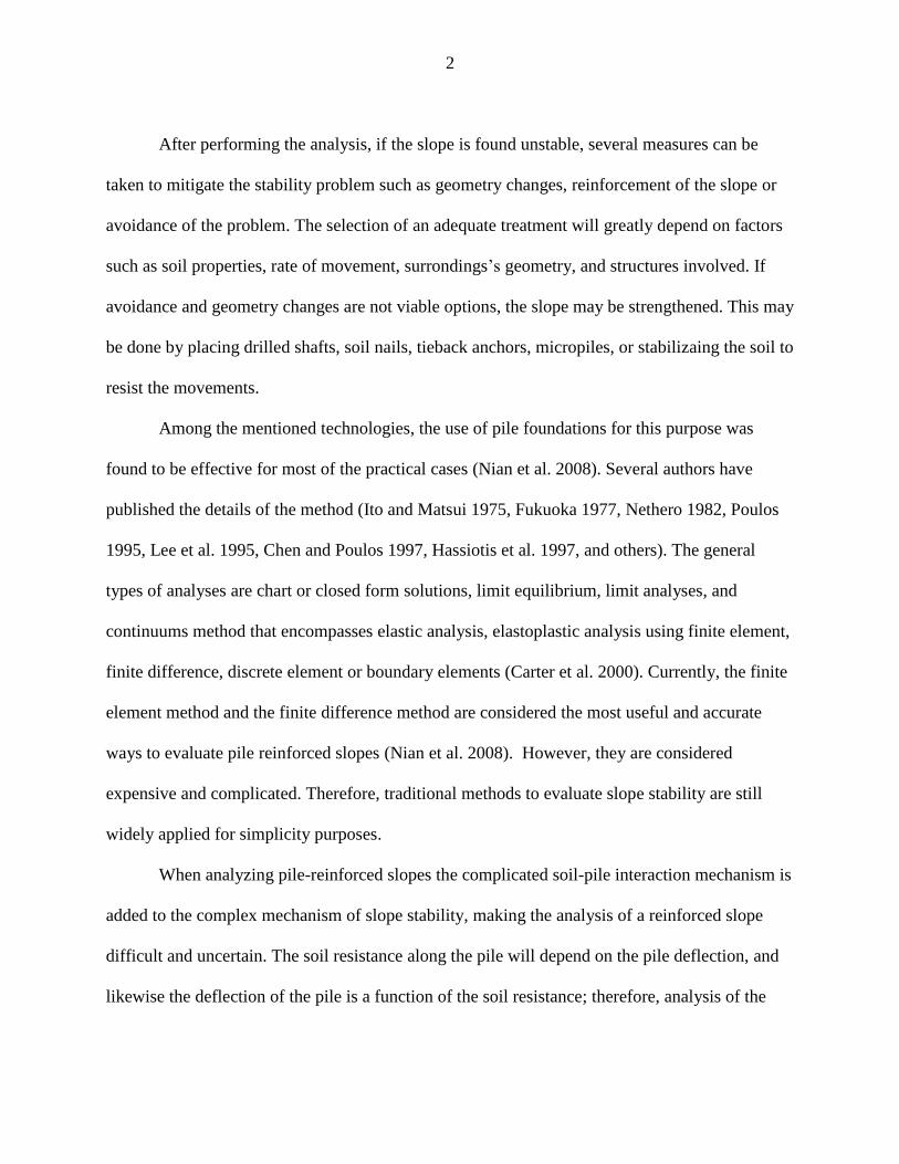
Among the mentioned technologies, the use of pile foundations for this purpose was
found to be effective for most of the practical cases (Nian et al. 2008). Several authors have
published the details of the method (Ito and Matsui 1975, Fukuoka 1977, Nethero 1982, Poulos
1995, Lee et al. 1995, Chen and Poulos 1997, Hassiotis et al. 1997, and others). The general
types of analyses are chart or closed form solutions, limit equilibrium, limit analyses, and
continuums method that encompasses elastic analysis, elastoplastic analysis using finite element,
finite difference, discrete element or boundary elements (Carter et al. 2000). Currently, the finite
element method and the finite difference method are considered the most useful and accurate
ways to evaluate pile reinforced slopes (Nian et al. 2008). However, they are considered
expensive and complicated. Therefore, traditional methods to evaluate slope stability are still
widely applied for simplicity purposes.
When analyzing pile-reinforced slopes the complicated soil-pile interaction mechanism is
added to the complex mechanism of slope stability, making the analysis of a reinforced slope
difficult and uncertain. The soil resistance along the pile will depend on the pile deflection, and
likewise the deflection of the pile is a function of the soil resistance; therefore, analysis of the
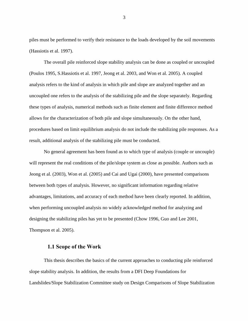
3
piles must be performed to verify their resistance to the loads developed by the soil movements
(Hassiotis et al. 1997).
The overall pile reinforced slope stability analysis can be done as coupled or uncoupled
(Poulos 1995, S.Hassiotis et al. 1997, Jeong et al. 2003, and Won et al. 2005). A coupled
analysis refers to the kind of analysis in which pile and slope are analyzed together and an
uncoupled one refers to the analysis of the stabilizing pile and the slope separately. Regarding
these types of analysis, numerical methods such as finite element and finite difference method
allows for the characterization of both pile and slope simultaneously. On the other hand,
procedures based on limit equilibrium analysis do not include the stabilizing pile responses. As a
result, additional analysis of the stabilizing pile must be conducted.
No general agreement has been found as to which type of analysis (couple or uncouple)
will represent the real conditions of the pile/slope system as close as possible. Authors such as
Jeong et al. (2003), Won et al. (2005) and Cai and Ugai (2000), have presented comparisons
between both types of analysis. However, no significant information regarding relative
advantages, limitations, and accuracy of each method have been clearly reported. In addition,
when performing uncoupled analysis no widely acknowledged method for analyzing and
designing the stabilizing piles has yet to be presented (Chow 1996, Guo and Lee 2001,
Thompson et al. 2005).
1.1 Scope of the Work
This thesis describes the basics of the current approaches to conducting pile reinforced
slope stability analysis. In addition, the results from a DFI Deep Foundations for
Landslides/Slope Stabilization Committee study on Design Comparisons of Slope Stabilization

4
Methods are reported. The comparative analysis will be performed by evaluating three cases
under uncoupled and coupled conditions. For performing the uncoupled analysis, two limit
equilibrium programs; SLOPE/W (Geo-Slope International 2010) and Slide 7 (Rocscience Inc.
2016), will be used in combination with LPILE 09.010 (Isenhower et al. 2016) for the analysis of
laterally loaded piles. On the other hand, FLAC 2D (Itasca 2005) and Phase2 (Rocscience Inc
2017) will be used for the coupled analysis as FD and FE software. The calculations from FLAC
were performed by Dr. Daniel Pradel as part of the DFI project. The strength reduction analysis
will be used to compare results from the geomechanical numerical analyses to the factor of
safety from limit equilibrium analyses.
1.2 Research Objectives
The two main objectives of this research are (1) investigate methods and accuracy of
advanced numerical modeling for slope stabilization methods (LEM, FEM and FDM) through
comparing three cases using different analysis approaches performing coupled and uncoupled
analysis, and (2) to provide recommendations for the selection of a given method for stability
analysis from a comparative basis regarding relative benefits when compared to traditional
methods.
1.3 Study Outline
The research outlined above is presented in four chapters. Chapter 2 provides background
information and reviews previous literature related to this study. Chapter 3 describes the
methodology and information regarding the three analyzed cases and the summary and
discussion of the results. Chapter 4 recaps the conclusions and key findings derived from the

5
analyses to report some suggestions for future research. Supporting materials are included as
appendices that follow the list of references that made possible the elaboration of this thesis.
Key Terms:
Slope stability, limit equilibrium, pile reinforced slope, numerical modeling in geotechnical
engineering, constitutive models.

6
CHAPTER 2. LITERATURE REVIEW
The basics of slope stability are presented in this chapter as well as the current methods
of analysis for stability problems. There are two (2) primary methods of analysis that are
currently used to estimate the stability of unreinforced and reinforced slopes: (1) methods based
on limit equilibrium analysis and (2) numerical-based analysis methods (such as finite element
analysis, strength reduction finite element method, and finite difference methods). The major
assumptions for each method, the advantages and disadvantages are discussed .The practical
applications that have been developed are mainly based on these theories of analysis with
variations and modifications that have been introduced by authors to address a specific aspect of
an analysis approach.
2.1 Basics of Slope Stability
Through the years, slope failures have been responsible for immeasurable economic
losses and casualties all around the world. According to Turner and Schuster (1996), landslides
or mass wasting represent a major component of numerous “multiple-hazard disasters”. Hence,
regarding the improvements in the prediction and mitigation of this type of events, a greater
amount of effort must be focused to increase the general understanding of the assessment of the
safety of slopes (natural or man-made slopes). This assessment is generally done by conducting
a slope stability analysis in which the major premise is to determine whether or not the soil
beneath the slope will be able to withstand loads without undergoing failure.
Commonly, stability is determined by balancing the resisting forces with driving forces.
The resisting forces, the soil strength, act opposite to the movement holding the soil or rock in
place while the driving forces, gravity through the soil weight, tend to pull the mass of soil or

7
rock down the slope. Hence, because both forces depend on soil properties, stability analysis is a
complex mechanism that remains a challenge for geotechnical engineers. The mechanism of
failure of slopes has been extensively studied and according to Duncan (1996) is considered one
of the areas of practice that has produced the most important advances in the complex behavior
of soils. However, they are gaps that need to be addressed in terms of selection of an appropriate
method of analysis for a particular given problem.
2.1.1 Types of Slope Failure
Stability can be defined as the safety of the earth mass against movement. Hence, slope
failure or mass wasting is the vertical and/ or horizontal soil displacement down slope of the
earth mass, soil, rock or debris (Turner and Schuster 1996). These movements have been
subdivided into six groups regarding the characteristics of the failure as shown in Figure 1
(Cornforth 2005, following the original work of Varnes (1978) and Cruden and Varnes (1996)):
a. Falls: vertical sliding of the surface particles in a slope. This involves large areas and the
movement is produced gradually between the mobile and fixed particles. The slide
surface is difficult to define.
b. Topples: rotation about some axis point in a forward direction due to the action of gravity
and forces applied by fluids or elements within the cracks.
c. Slides: refers to the downslope movement of a block of material, it could also be referred
as the movement of the slope body. It can be rotational and translational. The slip surface
penetrates deeply into the soils and can be easily defined.
d. Spreads: horizontal failure mainly related to shear and liquefaction.

8
e. Flows: faster movements of the natural slope such that the mechanism resembles the
movement of a viscous material. The slide surface is not easy to define and it is
developed in a short period of time.
f. Composites: a combination of any of the defined types. A composite failure may exhibit
least two kinds of movement at once in different locations of the displaced mass.
From Figure 1, slides are generally the better defined processes of slope failure and more
related to slope stability analysis.
Figure 1. Slope Movements Based on Classification by Varnes (1978) and Cruden and
Varnes (1996).

9
2.1.2 Potential Causes of Slope Failure
To remediate a problem the first step consists of understanding the factors that originated
the problem. In slope stability, failure can be caused by natural or man-made factors. In addition,
natural slopes have different issues than engineered and constructed slopes. Therefore, factors
such as geological history, formation, stress history, climate and man-made effects will play an
important role into the stability conditions of the slope.
Wright and Duncan (2005) summarized the common causes of slope failure. They stated
that the general processes causing failure will lie between increasing shear stress and decreasing
shear strength of the soil within the slope. Either of these mechanisms will lead to changing the
equilibrium between strength soil and shear stress. The most common triggering factors for the
mentioned processes are detailed as follows:
Increasing shear stress: In this category, field characteristics (could be natural or
constructed characteristics) and geological environment will be very important. For
instance, changes in slope geometry or water level fluctuations may either increase the
weight of the slope or decrease the lateral support. Moreover, water pressure
development on top of the slope, increasing loads on top of the slope (vegetation type and
amount may be included), and sudden shocks such as earthquakes, hurricanes, heavy
traffic or any triggered sudden movement should be accounted for when analyzing the
factors that can caused an increase in the shear forces that needs to be balanced by the
resisting forces.
Decreasing the shear strength: In this case, water level fluctuations also affect the
stresses values. Rise in the ground water may decrease the effective stress by pore

10
pressure increment. Seepage and leaching may also affect the slope equilibrium. In some
types of clays, swelling, strength softening, creep and decomposition by dissolution of
mineral may lead to strength loss. In general, dry clays have higher strength than wet
clays. Water level rising will saturate the soil and that will be the critical condition for
that kind of material. In the same way, in loose coarse grained saturated soils liquefaction
may occur under cyclic loading conditions causing considerable increases in pore water
pressure then decreases in effective stresses (Duncan and Wright 2005). On the other
hand, continue dropping or rising in water level may cause cracking and fractures that
result in strength loss on the cracking planes. Bedding planes developed naturally by
previous deposition are also susceptible to water due to the planar shape that allows water
to go through and reduced cohesion.
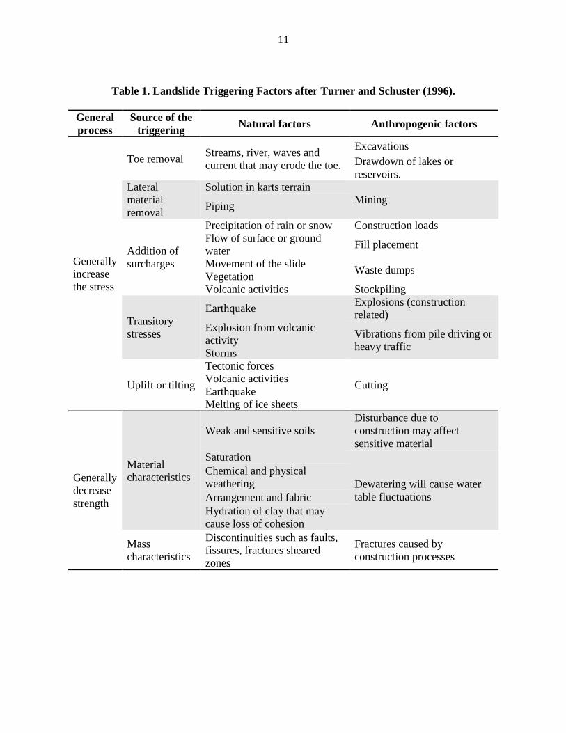
Table 1 contains the major triggering processes for slope failure divided into either natural or
man-made factors as presented by Turner and Schuster (1996). It must be pointed that factors
increasing stress may also decrease the strength of the soil in the slope.
11
Table 1. Landslide Triggering Factors after Turner and Schuster (1996).
General
process
Source of the
triggering Natural factors Anthropogenic factors
Generally
increase
the stress
Toe removal Streams, river, waves and
current that may erode the toe.
Excavations
Drawdown of lakes or
reservoirs.
Lateral
material
removal
Solution in karts terrain
Mining Piping
Addition of
surcharges
Precipitation of rain or snow Construction loads
Flow of surface or ground
water Fill placement
Movement of the slide
Vegetation Waste dumps
Volcanic activities Stockpiling
Transitory
stresses
Earthquake Explosions (construction
related)
Explosion from volcanic
activity Vibrations from pile driving or
heavy traffic Storms
Uplift or tilting
Tectonic forces
Cutting Volcanic activities
Earthquake
Melting of ice sheets
Generally
decrease
strength
Material
characteristics
Weak and sensitive soils
Disturbance due to
construction may affect
sensitive material
Saturation
Dewatering will cause water
table fluctuations
Chemical and physical
weathering
Arrangement and fabric
Hydration of clay that may
cause loss of cohesion
Mass
characteristics
Discontinuities such as faults,
fissures, fractures sheared
zones
Fractures caused by
construction processes

12
2.2 Slope Stability Analysis Methods
By understanding the potential causes of slope failure and their classification scheme, it is
easy to realize that to ensure stability, it is necessary to determine whether to increase the
resisting forces or decrease the driving forces. This simple concept corresponds to the basic of
most methods of analysis termed “limit equilibrium”. Those basic methods are intended to
determine a factor of safety involving equilibrium between the resisting and the driving forces.
There are also more sophisticated methods involving numerical analysis such as finite element
method and finite difference method incorporating the strength reductions technique. Each of
these procedures has different basic assumptions, advantages, and disadvantages that may need
to be taken into account when applied to a specific problem.
2.2.1 Limit Equilibrium
Limit plastic equilibrium is one of the simplest concepts for which several procedures
have been developed to conduct stability analysis. In general, limit equilibrium can be expressed
as
𝐹. 𝑆 =𝑠
𝜏
Where 𝜏 represent the shear stress in the soil, 𝑠 the soil shear strength and F.S. the factor of
safety to achieve a state of limit equilibrium (Huang 2014).
In limit equilibrium procedures, the shear strength is most often represented using the
Mohr-Coulomb equation as
𝑠 = 𝑐 + 𝜎𝑛 tanϕ
(1)
(2)
13
Where 𝑐 is cohesion, 𝜎𝑛 is normal stress, and ϕ is the angle of internal friction. Since 𝑐
and ϕ are known parameters of the soil, the shear stress along the failure surface can be
determined from Equation 2.
Although limit equilibrium based methods have been widely used due to their simplicity
and easy application, the accuracy and quality of the results could be compromised due to the
assumptions that need to be made to make most slope stability problems statically determined.
Hence, each procedure may yield different results for the same problem while satisfying
equilibrium conditions due to the different assumptions their authors have made.
The basic assumptions needed to conduct the analysis within a limit equilibrium procedure can
be summarized as:
Failure mechanism hypothesis (Assuming the shape and location of the failure surface
instead of determining it).
Soil movement is assumed as a rigid body block.
3-D effects are neglected.
Uniform location of shear stresses considering they are uniformly mobilized.
Currently, there are several limit equilibrium procedures, a summary of the most well know
was presented by Wright and Duncan (2005), Hopkins et al. (1975), and cited by Huang (2014).
From the literature review, the presented procedures were classified as single body methods and
slices methods. Moreover, from each category the most popular are presented.
2.2.1.1 Single body
Methods that consider equilibrium for a single free-body which means that do not separate
the soil mass. These are relatively simple to apply and are subjected to a range of applicability.
Among these methods can be found:
14
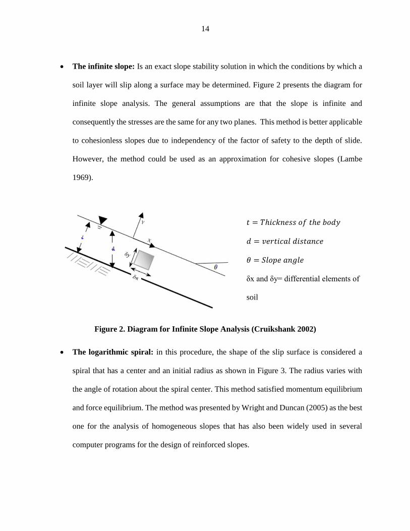
The infinite slope: Is an exact slope stability solution in which the conditions by which a
soil layer will slip along a surface may be determined. Figure 2 presents the diagram for
infinite slope analysis. The general assumptions are that the slope is infinite and
consequently the stresses are the same for any two planes. This method is better applicable
to cohesionless slopes due to independency of the factor of safety to the depth of slide.
However, the method could be used as an approximation for cohesive slopes (Lambe
1969).
Figure 2. Diagram for Infinite Slope Analysis (Cruikshank 2002)
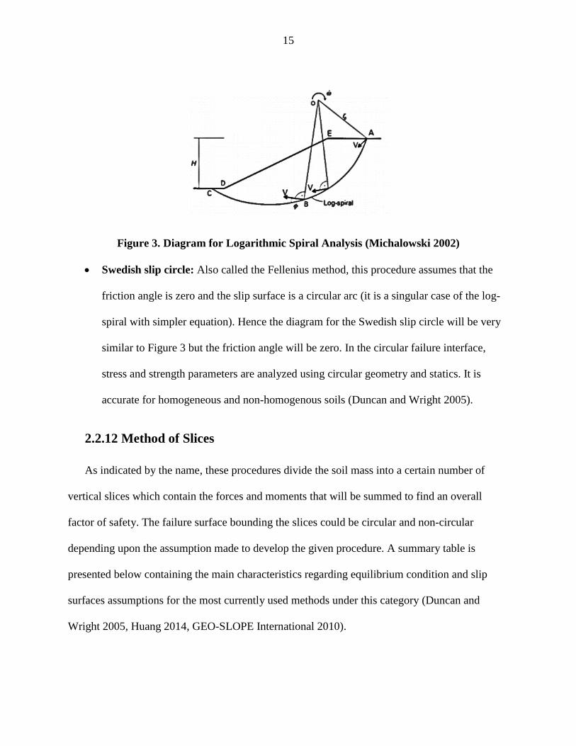
The logarithmic spiral: in this procedure, the shape of the slip surface is considered a
spiral that has a center and an initial radius as shown in Figure 3. The radius varies with
the angle of rotation about the spiral center. This method satisfied momentum equilibrium
and force equilibrium. The method was presented by Wright and Duncan (2005) as the best
one for the analysis of homogeneous slopes that has also been widely used in several
computer programs for the design of reinforced slopes.
𝑡 = 𝑇ℎ𝑖𝑐𝑘𝑛𝑒𝑠𝑠 𝑜𝑓 𝑡ℎ𝑒 𝑏𝑜𝑑𝑦
𝑑 = 𝑣𝑒𝑟𝑡𝑖𝑐𝑎𝑙 𝑑𝑖𝑠𝑡𝑎𝑛𝑐𝑒
𝜃 = 𝑆𝑙𝑜𝑝𝑒 𝑎𝑛𝑔𝑙𝑒
δx and δy= differential elements of
soil
15
Figure 3. Diagram for Logarithmic Spiral Analysis (Michalowski 2002)
Swedish slip circle: Also called the Fellenius method, this procedure assumes that the
friction angle is zero and the slip surface is a circular arc (it is a singular case of the log-
spiral with simpler equation). Hence the diagram for the Swedish slip circle will be very
similar to Figure 3 but the friction angle will be zero. In the circular failure interface,
stress and strength parameters are analyzed using circular geometry and statics. It is
accurate for homogeneous and non-homogenous soils (Duncan and Wright 2005).
2.2.12 Method of Slices
As indicated by the name, these procedures divide the soil mass into a certain number of
vertical slices which contain the forces and moments that will be summed to find an overall
factor of safety. The failure surface bounding the slices could be circular and non-circular
depending upon the assumption made to develop the given procedure. A summary table is
presented below containing the main characteristics regarding equilibrium condition and slip
surfaces assumptions for the most currently used methods under this category (Duncan and
Wright 2005, Huang 2014, GEO-SLOPE International 2010).

16
Table 2 shows the different assumptions of each method and their range of applicability. In
fact, methods developed based on circular slip surfaces such as Ordinary method and Simplified
Bishop method are restricted to simple geotechnical problems. For instance, problems related to
multilayered systems with a combination of weak and strong layers may not exhibit circular slip
surface shape. Hence, soil properties and slope geometry will influence the selection of the
procedure to guarantee the accuracy of the results.
On the other hand, as methods become more able to be applied to different conditions its
complexity also grows. In this regard, The Bishop and Ordinary method can easily be calculated
by hand while Morgenstern-Price’s, considered applicable to all slopes geometries, is not
feasible for hand calculation.
Many different types of software have been developed based on limit equilibrium methods
such as Slide, SLOPE/W, Hydrus, SVSlope, DotSlope, Galena, GSlope, Clara-W, TSlope3, and
Autoblock (for rock slopes), and specifically programmed loops that enable analysis of a given
situation using different procedures.

17
Table 2. Assumptions Equilibrium Condition for Slices Limit Equilibrium Procedures
Method
Equilibrium
condition that
satisfies
Interslice forces
included/inclination Slip surfaces shape
Ordinary
method of
slices or
Fellenius
Moment
equilibrium
(overall)
No interslice forces Circular
Simplified
Bishop
Moment
equilibrium
(overall)
Normal/Horizontal Circular
Original
Spencer
Moment and force
equilibrium
(overall)
Normal and Shear /Parallel
and inclined x angle with the
horizontal
Circular and Non-
circular
Janbu’s
Simplified
Force equilibrium
(each slice) Normal/Horizontal
Circular and Non-
circular
Morgenstern-
Price
Moment and force
equilibrium (each
slice)
Parallel between them
/Unknown determined through
a function
Circular and Non-
circular
Force
equilibrium(each
slice)
Normal and Shear / Average
of ground surface and Failure
surface
Circular and Non-
circular
Corps of
Engineers (1)
Force equilibrium
(each slice)
Normal and Shear / Parallel to
the slope of a line from crest to
toe Circular and Non-
circular Corps of
Engineers (2)
Normal and Shear / Parallel to
the slope of the surface and
same for all slices
Janbu
Generalized
Moment and force
equilibrium (each
slice)
Normal and Shear /Assumed
arbitrarily
Circular and Non-
circular
Sarma –
vertical slices
Moment and force
equilibrium
(overall)
Normal and Shear (Include
unknown seismic coefficient) /
Function
Circular and Non-
circular
Spencer
Moment and force
equilibrium (each
slice)
Normal and Shear
interslice/Parallel and inclined
x angle with the horizontal
Circular and Non-
circular
18
2.2.2 Numerical Analyses
Although numerical approximation as a solution for complicated problems is a technique
that has been around over a hundred years, in the past because of the complexity of the
geotechnical materials (e.g. soil and rocks) this kind of solutions were considered very difficult
to apply requiring significant computer power (Desai and Christian 1977). However, with the
development of computers, the application of numerical techniques to geotechnical problems
started to grow. Among the available numerical techniques, the finite element, and finite
difference methods are the most common applied in the geotechnical field.
2.2.2.1 Finite Element Method
The Department of the U.S Army Corps of Engineers in their Engineering and Design
Geotechnical Analysis by the Finite Element Method (Kamien 1995), defined the Finite Element
Method (FEM) as “a numerical technique” that can be used in the geotechnical field to solve
geotechnical problems. This technique has enhanced the capacity to perform more complex
analyses such as analysis of deformations of slopes and embankments, determination of stresses
and movements in excavations as well as tunneling, earth pressure structures among other
complex geotechnical problems.
FEM are based on discretization of the problem which means the division of the problem’s
geometry into several small elements. Regarding the use of FEM in slope stability problems
several authors (Carter et al. 2000, Duncan 1996, Duncan 1998, Christian 1998) have presented
its advantages when compare with traditional methods as follows:
Soil strength-stress relationship (non-linear material behavior) can be analyzed.
Displacements can be determined and construction sequences can be modeled.

19
Soil structure interaction when performing reinforced analyses can be studied.
Changes in soil behavior can be simulated.
No assumption of failure mechanism, interslice forces, and shape of the slip surface are
needed to conduct the analysis.
Regarding the disadvantages, skills such as geotechnical engineering understanding, relative
large computer storage, time investment to developed a model, and cost are crucial to achieving
a successful analysis. Concerning the available software’s, they are several systems designed
specifically for the geotechnical field. Those are PLAXYS, SIGMA, and CRISP. Moreover,
general-purpose programs such as ABAQUS, ADINA, SAP, and ANSYS can also be used for
geotechnical problems and also special programs designed for particulars cases are also currently
available.
2.2.2.2 Finite Difference Methods
Finite difference methods (FDM) as indicated by their name are based on finite difference
formulation. In this method, the problem is analyzed by time steps, stresses and strains are then
computed for each time step by either forward, backward or central differences. The FDM is the
oldest numerical technique introduced in the 1930s with the solution of mathematical physics
problems by means of finite difference (Thomã 2001). As in the FEM, FDM can also simulate
the soil stress-strain relationship hence assumptions needed in traditional slope stability methods
(LEM) are eliminated. Hence, complex problems and more realistic results are found from this
kind of analysis. According to Carter et al. (2000), the FDM could be considered more user-
friendly than FEM regarding the inputs for soil modeling. However, given the type of algorithms
employed, the method is less efficient for linear or moderately nonlinear problems. Even though
20
both FEM and FDM are numerical methods and both need constitutive models to represent the
soil behavior under applied stresses, several differences among the methods can be mentioned.
The major differences are:
FDM does not require matrix operations for solution.
FEM comes from mechanical and structural analysis being generalized to be applied to
continuous media like soils.
Field variables vary using specified functions in the FEM, while for FDM the field
variables are defined at nodes and not in between.
FDM use an explicit method by solving in time steps. FEM implicitly operates matrix by
trial and error until the error is minimized.
Regarding the available programs, the most popular FDM based program is FLAC. The
FLAC code was developed by ITASCA (1996) and consists of an explicit finite difference code
that simulates soil or rock structures which experience plastic flow when their yield limit is
reached (Kourdey et al. 2001).
2.2.2.3 Strength Reduction Method
The Shear Strength Reduction (SSR) method is a procedure used in FEM/FDM in which
the factor of safety is obtained by weakening the soil in steps in an elastic-plastic finite element
or finite difference analysis until the slope “fails” (Dawson et al. 2015, Griffins and Lane 1999,
Pradel et al. 2010, Fu and Liao 2010). According to the literature, the method was first proposed
by Zienkiewicz et al. (1975). In this method, the factor of safety for a slope is considered to be
the ratio of the actual shear strength to the lowest shear strength of a rock or soil material that is
required to maintain the slope in equilibrium. Thus, the factor of safety is considered to be the

21
factor by which the soil strength needs to be reduced to reach failure. Numerically, the failure
occurs when it is no longer possible to obtain a converged solution.
For Mohr-Coulomb material the shear strength reduced by a factor (of safety) F is determined as
𝜏
𝐹=𝑐′
𝐹+𝑡𝑎𝑛𝜑′
𝐹
Where;
𝑐∗ =𝑐′
𝐹 𝑎𝑛𝑑 𝜑∗ = 𝑎𝑟𝑐𝑡𝑎𝑛 (
𝑡𝑎𝑛𝜑′
𝐹)
are the reduced Mohr-Coulomb shear strength parameters.
Regarding the advantages of the application of the SSR, Rocnews (2004) has presented a
summary of the major advantages as:
It eliminates the need for a priori assumptions on failure mechanisms as in LEM (the
type, shape, and location of failure surfaces). This also minimizes the expertise required
in finding critical failure mechanisms.
Elimination of arbitrary assumptions regarding the inclinations and locations of inter-
slice forces.
Monitoring of the development of failure zones from localized areas until the total slope
failure is automatically achieved.
Expected deformations at the stress levels found in slopes can be predicted.
Despite, all the mentioned advantages SSR, its adoption has been limited primarily because
of inadequate experience that engineers have with the tool for slope stability analysis, and the
limited published information on the quality/accuracy of its results (Hammah et al. 2005).
(3)
(4)

22
2.2.2.4 Modeling
Numerical modeling originates from applying numerical analyses to represent a real
physical problem. A model should characterize as close as possible the real conditions that are
intended to be analyzed. However, because of the inherent difficulties that embody a numerical
analysis, simplifications and engineering judgment are very important factors to achieve accurate
results. The objective for modeling must be clearly defined before the model creation. As
expressed by Marr (1999) “Know the answer before you start” should be the guiding rule when
modeling (FEM). This is because errors in models involving quite complex mechanisms are
difficult to detect, so an estimation of the answer may help to evaluate comparatively the FEM or
FDM results. Thus, since the process has been defined as complex some of the reasons that
justify undertaking a thorough modeling effort are: make quantitative predictions, compare
alternatives, identify governing parameters, understand processes, and train our thinking (Geo-
Slope 2013). For instance, problems related to complex geometries and material variations will
be better analyzed by modeling than by using traditional methods (such as limit equilibrium
method).
Numerical modeling has been pointed out as a skill that helps to overcome many
limitations related to oversimplified assumptions for soil properties and boundary conditions in
the geotechnical field. Problems such as non-linear soil properties, soil-structure interaction, and
seepage among other can be better analyzed. However, the necessity for understanding geology,
site conditions, and the phenomena that control the construction processes to account for a
realistic point of view is still needed to perform an adequate analysis. Hence, numerical
modeling application does not substitute the basic requirements of a good geotechnical engineer
(Duncan 1998). Therefore, using software should be seen as part of the modeling processes tied

23
to conceptualization and interpretation of the results. It is then elemental to determine whether or
not modeling will be needed for a problem, the means by which the model will be constructed,
the available information to create the model, and what will be the model assessment.
If the conditions while modeling are not well-understood errors may take place. Some of
the reasons for these errors could be mathematical model errors, conceptual errors, input data
errors, numerical errors and interpretation errors. To prevent the occurrence of errors several
factors should be taken into account when constructing a numerical model, these factors will be
detailed in the following section.
Important Factors for Modeling:
A model may represent the real condition of the problem that is being analyzed in the
most accurate way possible. Hence there are a series of factors that may help to achieve a
successful model. Among these factors are the key aspects of the construction of the model, what
kind of components should be modeled, the way the model will represent certain field
conditions, the way the geomaterials will be represented by the model, and the way results will
be evaluated and compared with the reality.
Model Building
Before starting to build a model, a meticulous characterization of the site or problem
conditions must be performed. Understanding the mechanisms and factors involved in the
problem that will be analyzed as well as estimation of the result will lead to successful
application of the desired numerical analysis. For instance, water conditions, soil boundary
24
conditions pore water pressures, and geometry are some of the factors that should be clearly
visualized before starting modeling.
Regarding the geometry, generally, the common belief is that adding every single detail
to a model will make it more accurate. However, that increases the complexity and possibly the
inaccuracy of the results. Therefore, the important components or most significant aspects that
may influence the results for which the model is being built should be selected (Geo-Slope
2013). For instance, very small layers of soils embedded into a large stratum with similar
properties could be simplified as one stratum. Moreover, physical elements that do not affect the
results can be simplified or eliminated from the model, for instance, a rounded structural element
could be linearized.
Constitutive Models
Another factor playing a key role in model building is the characterization of the soil
properties involved in the studied case. Constitutive models have been developed with the
objective of representing the relationship between stress and strength, and perhaps time, of a
given material for numerical analysis (Lade 2005). The quality and accuracy of any given
numerical analysis such as finite element method or finite difference method applied to a
geotechnical problem will greatly depend on the representation of the constitutive relationship
used. Therefore, it can be said that constitutive model, its selection, and accuracy have a major
responsibility in geotechnical finite element/ finite difference analysis. As presented by several
authors (Desai and Asce 1985, Duncan 1996, Carter et al. 2000, Lade 2005), there are a large
variety of constitutive models. However, not all types of model can be correctly applied to all
25
types of soils and, moreover, each method has been developed over a range of stresses and
strains intended to represent the real condition to which the material will be exposed.
The mathematical representation of soil properties is not an easy task because of soils’
complex nature and behavior under loading conditions. In this regard, several theories of
material behavior perfectly fit with other construction materials such as steel or concrete. Those
two mentioned materials can easily be represented as elastic or elastic-perfectly plastic. In the
soils’ case, stress-strain behavior is not linear, volume change takes place during shearing and
different materials will behave differently whether the range of stresses is close or far from
failure and the material is loose or dense. Hence, to develop realistic models that can duplicate
the important aspects of the soil stress-strain behavior subjected to different loading conditions, it
is required to perform advanced experiments to study soil behavior versus loading within applied
mathematical frameworks of elasticity and plasticity theory.
Duncan (1996) presented a summary of the currently available stress-strain relationships
that can be selected for a numerical analysis. He highlights the association between accuracy and
complexity that may be analyzed when selecting a given model. In this regard, the alternatives
include, linear elastic, multilinear elastic, hyperbolic (elastic), elastoplastic, and elasto-
viscoplastic behavior.
Linear Elastic: This theory is based on Hooke’s law. Immediate deformations and
settlement are calculated from an elastic modulus estimated from a stress-strain curve
(Lade 2005). The major advantage of this kind of model is the simplicity and the small
number of parameters needed (Poisson’s ratio and Young’s modulus). However, in
elasticity theory when an applied stress is removed, the material returns to its undeformed
state. Hence, soils are fundamentally frictional materials so volume change will take
26
place during drained shearing. Hence, this theory is not a good model in representing the
actual soil behavior.
Multilinear Elastic: In this model more than one straight line is used to model stress-
strain curves, and modulus reductions. This is done with the objective of improving the
accuracy of the values from the lab test (Duncan 1996).
Hyperbolic Elastic: This method relates stress increments to strain increments (as in
Hooke’s law). However, in this method stresses and moduli are systematically related.
Elastoplastic: In this kind of model, yield function and surface, plastic potential, elastic
properties and surface, and hardening must be characterized. Since in this model the
stress-strain relationship is more complex than in elastic models, they are expected to
capture more closely the real behavior of soils under high stress levels (closest to failure).
Duncan (1996) pointed that if the conditions are not close to failure no major advantage
will be found in applying this model.
Elastic-perfectly plastic: The Mohr-Coulomb model is the simplest well know elastic-
perfectly plastic model. In this model, the soil stress-strain behaves linearly in the elastic
range (based on Hooke’s law). Hence, in that range the Poisson ratio and Young’s
modulus are the representing parameters. On the other hand, in the perfectly plastic zone
the behavior is based on the Mohr-Coulomb failure criterion. The friction angle, ϕ, the
cohesion, c, and the dilatancy angle, Ψ, are the parameters that define the failure criteria
(Ti et al. 2009).
Hence, when selecting a constitutive model a key factor to be considered is the type of
material that will be represented. For instance, the density of the material will be important to

27
determine its behavior under loading. Some models represent the behavior of soft clays better
than sands (frictional materials must be represented with a model developed over the non-
associated flow rule (Lade 2005)). This is because in some cases, if soils are not stressed close to
failure, they could be represented as linear elastic materials. Thus, models developed under
elastic general assumption can be used.
Another vital factor is to understand the basis for the model’s development and its
shortcomings, how the relationship stress-strain was considered. For example, hyperbolic models
relate stress and strain by a systematic method and the parameters values can be determined by
laboratory test while linear elastic models use just two elastic parameters and they are not a good
representation of the actual soil behavior. However, as complexity is also a factor to be
considered some simplifications can be done regarding the type of project and the purpose of the
analyses. Construction sequence is also an important detail in selecting the constitutive model
(Duncan 1996). In this regard, slow a construction assumption will indicate little development of
excess pore pressure, which may affect long-term stability; these effects will be different from
one model to another (USACE 1995).
The number of parameters involved in the model should be also considered. Generally, the
larger the number of parameters, the more flexible and versatile the model is considered. In
addition, parameters can be easily determined when compared with experimental results.
However, the calibration process of the model will influence the complexity and cost if the
model demands non-standard and complex experiments for calibration, which will increase the
cost (Lade 2005).
Finally, numerical analyses have enabled the geotechnical field to increase the ability to
perform more accurate analysis. However, the effort to increase the ability to understand and

28
represent site conditions in modeling may be excessive. This is significantly true for the
constitutive models’ case where complex ground conditions, inadequate site characterization,
and inadequate data for appropriate constitutive models still remain as reasons for potential
limitations on the applicability of FEM to geotechnical field. As expressed by Whittle (1999) the
profession needs to invest more resources on validation of the current capacities and this includes
current constitute models before the development of new ones.
Model Calibration and Validation
Generally speaking, calibration is defined as correlation or standardization of a modeled
reading with those from known results. Hence, when talking about model calibration, the
simulated data must be matched with observed values by varying the inputs to account for
unknown or uncertain conditions. The main objective of calibration is to guarantee that a certain
model will represent the studied conditions as closely as possible. In the same way, validation is
needed to define reliable models when numerical analysis has been conducted. Reference points
regarding domain of the analysis, type of model to be applied, type of tests that will be
conducted to validate the model, and replicability of the results are very important to determine if
the strength properties of the in situ ground are accurately represented in a model (Carter et al.
2000).
29
2.3 Reinforced Slopes
After the factor of safety for an unreinforced slope has been determined, several
approaches for remediation can be applied if the calculated value does not meet minimum safety
requirements. These remediation techniques can generally be categorized as follows; (1) avoid
the problem, (2) decrease the shear stress or driving forces, or (3) increase the shear strength or
resisting forces (Turner and Schuster 1996). Regarding the degree of stabilization required and
the actual condition of the slope, other approaches such as maintenance, observation, and do
nothing could also be followed. Maintenance and observation will be generally focused on the
monitoring and temporary treatment of slow moving landslide. On the other hand, the do nothing
could be plausible when a slow constant trend resulting for years of monitoring is seen.
However, the understanding of the later consequences must be ensured (Cornforth 2005). A
summary of approaches to mitigate slope stability problems is presented in Table 3.
Slopes containing structural elements that increase the ability of the slope to withstand
movements are called reinforced slopes. Methods by which a slope can be reinforced are
presented in Table 3 and will generally follow under the increasing the resisting forces approach.
The resisting forces can be increase by either applying external forces or increasing the internal
strength of the soil in the failure zone (Turner and Schuster 1996). The methods in the first
category will focus on providing enough external restraint to prevent the movement. On the other
hand, to increase internal strength, reinforced soil and in situ reinforcement has been used. The
selection of a particular remediation method will vary in terms of available physical space,
geometry, surrounding structures cost, desirable remediation degree and material characteristics.

30
Table 3. Remediation Methods for Slope Stability Problems, Turner and Schuster (1996)
Category Procedures Limitations
Do nothing “No action”
Non effective if long term catastrophic failure
Applicable to slow moving or stable accelerating
slopes
Avoid the
problem Relocate project
Should be studied during planning
Cost impact regarding location selected
No cost effective if design is complete
Maintenance
Activities such as
removing materials,
closing areas, etc.
Limited to slow moving landslides
Will be temporary then it will need to be re-done
Monitoring Inclinometers, surface
survey points, etc. Limited to slow moving landslides
Decrease
driving
forces
Change the grade
Could affect sections of adjacent roadways
Not always available physical space for change
in geometry
Drain surface Will only correct surface infiltration or seepage
due to the surface infiltration
Drain subsurface Will depends on permeability of the sliding mass
Reduce weight Requires right-a-way and lightweight materials
Produce excavation waste that need to be handle
Increase
resisting
forces
Use buttress or
counterweight fills;
toe berms
Could not be effective in deep-seated landslides
Requires right-a-way
Could require a firm foundation
Use structural system Could not handle large deformations
Should penetrate well below sliding surface
Install anchors Requires a firm foundation to resist the shear
forces of by the anchors tension
Drain subsurface Will depend on permeability of the sliding mass
Use reinforced
backfill Requires durability of reinforcement
Install in situ
reinforcement
Requires long-term durability of nails, anchors,
piles, micropiles
Use biochemical
stabilization
Limited to the height of the slope
Affected by climatic conditions
Treat chemically Long-term effectiveness is still in evaluation
Could be affected and affect the environment
Use electrosmosis Requires maintenance and constant direct current
Could be expensive
Use thermal
stabilization
Require expensive and carefully designed system
Could be expensive

31
2.4 Pile Reinforced Slopes
Among the mentioned methods in section 2.3, this thesis will focus on the evaluation of
stability of reinforced slopes by means of pile elements. Piles have been found to be an effective
way to stabilized slopes (De Beer and Wallays (1970), Ito and Matsui (1975), Cai and Ugai
(2000), Hassiotis et al. (1997), Lee et al. (1995), Poulos (1995), Chen and Poulos (1997)).
However, evaluating the stability of pile reinforced slopes represents a major challenge in the
field, not only because of the several uncertainties that take place in the phenomenon, but also
because the mechanism soil-stabilizing pile is very complex. Moreover, no widely acknowledged
method for analyzing and designing the stabilizing piles has yet to be presented (Chow 1996).
To evaluate the stability of pile-reinforced slopes in the same way as for unreinforced
slopes, the basis of the analysis is to determine the factor of safety. The factor of safety has been
defined previously as the ratio between resisting forces and the driving forces along the failure
surface. However, to determine the critical failure surface in a reinforced analysis, two analyses
should be conducted for the same slope (1) determine the factor of safety of the unreinforced
slope, and (2) determine the factor of safety for the reinforced slope, because the failure surface
is not constant and tends to vary while accounting for the pile effects (Ausilio et al. 2001, Ito and
Matsui 1975, Lee et al. 1995). This means that other critical surfaces could be generated as a
consequence of the pile placement. Therefore, an iterative process should be conducted.
Moreover, when analyzing pile-reinforced slopes, study of the piles must be also
performed to verify the resistance of the pile to the loads developed by the soil movement
(Hassiotis et al. 1997). Hence, the overall analysis can be done as coupled or uncoupled. The first
one refers to the kind of analysis in which pile and slope are analyzed together and the second
one refers to the analysis of stabilizing pile and slope stability separately. Regarding these types
32
of analysis, numerical methods such as finite element and finite difference method allow for the
characterization of both pile and slope stability simultaneously. On the other hand, procedures
based on limit equilibrium analyses do not include the stabilizing pile responses on the analysis.
As a result, additional analysis of the stabilizing pile must be conducted.
2.4.1 Analysis of Reinforcing Piles
Piles used to stabilize slopes will be subject to lateral forces developed from the
movement of the surrounding soil. In general, piles subjected to lateral forces can be divided into
“passive piles” and “active piles” (De Beer and Wallays 1970, Ito et al. 1979). According to Ito
et al. (1979), the passive piles case is more complex than the active one due to the interaction
between the piles and the soil that generates the lateral forces.
The general design approach for stabilizing piles follows a procedure presented by
(Viggiani 1981) in which three main steps are followed; (1) evaluate the needed shear force to
increase the safety of factor of the slope; (2) evaluate the maximum shear force provided by each
pile; (3) select the number of pile and the optimum location. This will be discussed in more detail
in section 2.4.2. The first step is conducted by performing a stability analysis with a target factor
of safety. From the difference between the actual factor of safety (unreinforced) and the target
value, the stabilizing force required can then be found.
The second step is addressed by performing a lateral response analysis. In this regard,
several empirical and numerical methods have been presented. These methods can be
categorized as (1) pressure-based methods (De Beer and Wallays 1970, Ito and Matsui 1975,
Hassiotis et al. 1997); (2) displacement-based methods (Poulos 1995, Chen and Poulos 1997),
33
and (3) continuum methods (Cai and Ugai 2000, Kanungo et al. 2013). The general basis of the
methods for analyzing pile responses will be presented:
2.4.1.1 Pressure-based Method
The piles subjected to lateral pressures are analyzed as passive piles based on the method
developed by Ito and Matsui (1975). This method was developed assuming that the soil
surrounding the pile undergoes two plastic states: (1) plastic deformation and (2) plastic flow.
The first stage satisfies the Mohr-Coulomb yield criterion and in the second one, the ground is
considered as a visco-plastic solid. Hence, plastic deformation can be compared to hard soil
layers and plastic flow could be compared to creep deformation of a soft layer. The general
assumptions of the plastic deformation theory by Ito and Matsui (1975) are:
1. AEB and A'E'B' are two sliding surfaces that occur making an angle of (𝜋
4+𝜑
2) with the
x-axis, when the soil layer deforms as presented in Figure 4.
2. In the area AEBB'E'A' the soil is in a state of plastic equilibrium. Thus, the Mohr-
Coulomb yield criterion applies.
3. The active earth pressure acts on lane AA’.
4. The soil layer is in plane-strain respect to depth direction.
5. The piles are considered rigid
6. The frictional forces on surfaces AEB and A'E' B' are neglected, when the stress
distribution in the soil AEBB'E'A' is considered.
34
Then, assuming the Mohr-Coulomb yield criteria rules the plastic deformation of the EBB’E’
and AEE’A” areas, the pressure acting on the piles per unit thickness (q) will be determined
as:
𝑞 = 𝐴𝑐
(
1
𝑁𝜑 tan𝜑𝑒[𝐷1−𝐷2𝐷2
𝑁𝜑 tan𝜑 tan(𝜋8+𝜑4)]−2√𝑁𝜑 tan𝜑−1 +
2 tan𝜑 + 2√𝑁𝜑 +1
√𝑁𝜑
√𝑁𝜑 tan𝜑 + 𝑁𝜑 − 1
)
− 𝑐
(
𝐷1
2 tan𝜑 + 2√𝑁𝜑 +1
√𝑁𝜑
√𝑁𝜑 tan𝜑 + 𝑁𝜑 − 1− 2𝐷2
1
√𝑁𝜑
)
+𝛾ẑ
𝑁𝜑𝐴𝑒
[𝐷1−𝐷2𝐷2
𝑁𝜑 tan𝜑 tan(𝜋8+𝜑4)]−𝐷2
Where 𝑐 is the cohesion intercept, 𝐷1 is the center to center distance between piles, 𝐷2 opening
between piles, 𝜑 is the angle of internal friction of the soil, 𝛾 the unit weight of the soil, ẑ the
depth from the ground surface and 𝑁𝜑 and A are:
𝑁𝜑 = 𝑡𝑎𝑛2 (𝜋
4+𝜑
2)
𝐴 = 𝐷1 (𝐷1
𝐷2)√[𝑁𝜑 tan𝜑+𝑁𝜑+1]
(5)
(7)
(6)

35
Figure 4. State of Plastic Deformation in the Ground just Around the Piles (after Ito and
Matsui 1975)
Furthermore, the general assumptions of the plastic flow theory Ito and Matsui (1975) are:
1. Figure 5 shows the soil between two piles ACDFF’D’C’A’ flowing at velocity v1. It is
assumed that a visco-plastic flow will occur just around the piles in the AEBB’E’A’ and
that the flow direction is always centripetal towards the EBB’E’ zone.
2. The soil layer is considered in steady state behaving as a Bingham fluid with yield stress
𝜏𝑦 and plastic viscosity 𝑛𝑝. In addition, the flow is considered in the depth direction.

36
3. The forces applied on the portions GH and G’H’ by small soil elements can be obtained
by summing the force due to earth pressure and the viscous flow of the element through a
channel with width GG’.
4. Piles were assumed to be rigid.
Hence assuming the soil flows uniformly at averages velocities 𝑣1, 𝑣𝑟 𝑎𝑛𝑑 𝑣2 through BB’,
GG’ and EE’ and substituting and integrating the shearing force acting on the small portions GH
and G’H’ and the velocity 𝑣𝑟 the force acting on the surface is obtained. The lateral force acting
on the pile per unit thickness (p) is finally determined as:
𝑝 = √2𝑚𝜏𝑦
(
√1 +
𝑚
2𝜏𝑦𝐷22 −√1 +
𝑚
2𝜏𝑦𝐷12 + log
𝐷1 (1 + √1 +𝑚
2𝜏𝑦𝐷12)
𝐷2 (1 + √1 +𝑚
2𝜏𝑦𝐷22))
+ (𝐷1 − 𝐷2) ([√2 − 1]𝜋𝑚
8𝐷22 + (√2 − 1)√(
𝜋2𝑚
8𝐷22) +
𝜋2𝑚𝜏𝑦
4𝐷22 +
𝑚
𝐷1𝐷2+ √2𝜏𝑦
− 2𝑐 + 𝛾𝑧)
Where 𝑐 is the cohesion intercept, 𝐷1 is the center to center distance between piles, 𝐷2
opening between piles, 𝜏𝑦 is yield stress, 𝑛𝑝 is plastic viscosity, 𝛾 the unit weight of the soil, ẑ
the depth from the ground surface and m is :
𝑚 = 16𝑛𝑝𝑣1𝐷1
𝜋2.
(8)
(9)
37
Figure 5. State of Plastic Flow in the Ground just Around the Piles (after Ito and Matsui
1975)
Because the presented method considered a fixed critical surface when in fact the critical
surface will vary by the piles addition, (Hassiotis et al. 1997, Ausilio et al. 2001, Ito and Matsui
1975, Lee et al. 1995), the piles were considered to be rigid, and the soil was assumed to be able
to plastically deform around the piles, the method has limited applicability by not representing
the actual soil/pile interaction (Jeong et al. 2003). Ito and Matsui (1975) concluded that, in the
theory of plastic deformation, the lateral force will increase as c and ∅ increases. On the other
hand, in the theory of plastic flow, the lateral force will increase as increasing yield stress and
plastic viscosity but the change is not significant for yield stress changes. For both theories, the

38
lateral forces agree in order of magnitude with the observed values. The lateral force should be
estimated by integrating equation (5), from the theory of plastic deformation along the depth of
the soil layers, when piles are top restrained
2.4.1.2 Displacement-based Method
This method is based on determining the lateral pile response to the lateral ground
movements. Hence, the lateral soil movement needs to be determined for its application. The
method could use either measured inclinometer data or analytical results by finite element
approach to simulate the soil/pile interaction mechanism. Poulos (1973) presented a useful
approach to determine laterally loaded pile responses using the soil/pile interaction analysis in
which the movement of the soil through the pile is considered.
The presented approach uses a simplified boundary element where the pile is modelled as
elastic beam and the soil as an elastic continuum. The lateral displacements for each pile element
are associated with its bending stiffness and the horizontal pile/soil interaction stresses. A
limiting lateral pile/soil stress can be specified allowing local failure of the soil to obtain a
nonlinear response. This analysis must be solved by a computer program since a set of equations
should be solved for incremental analysis and incremental pressures.
According to Poulos (1995) the lateral response analysis requires knowledge of lateral soil
modulus distribution, free-field horizontal soil movements and distribution with depth of the
limiting soil/pile pressure. The basic problem of a pile in an instable slope is presented in Figure
6. It has been assumed that the upper soil moves as a rigid body downslope direction, a small
zone below is called drag zone and the stable zone is stationary. The key soil parameters
involved in the approach are the Young’s modulus and the limiting lateral pressure. These

39
parameters are mainly assessed by correlation, therefore, their values may carry some
inaccuracy.
Figure 6. Basic Problem of a Pile in Unstable Slope after Poulos (1995)
The theoretical analysis from Poulos (1995) revealed the existence of four pile modes of
failures; (1) flow mode; (2) short-pile mode; (3) intermediate mode; (4) long-pile failure. The
first three modes correspond to modes of failure of the soil while the last one refers to the failure
of the pile itself. The soil modes of failures are illustrated in Figures 7 to 9.
1. Flow mode: The critical sliding surface is shallow and the unstable soil flows around the
pile.
2. Short-pile mode: The critical sliding surface is deep and the length of the pile in the
unstable soil is shallow and full mobilization of the soil strength on the stable layer
happens.
3. Intermediate mode: The stable and unstable soil strength is mobilized along the pile
length.
4. Long-pile failure: The maximum bending moment reaches the yield moment of the pile
section and consequently the pile yields.

40
Poulos (1995) determined that the resistance provided by the piles to stabilize the slope
will be greater if the governing mode of failure is the intermediate one. Additionally, proper
reinforcement of the pile is needed to avoid the long-pile failure.
Most of the available methods to analyze laterally loaded piles are based on the p-y
method. This method uses finite element difference for solving the nonlinear four order
differential equation of a bean-column system on an elastic foundation. Equation 10 was
originally presented by Hetenyi (1946) and posteriorly modified by Poulos (1973) and Byrne et
al. (1984) to analize the pasive case that is when pile are subjected to lateral movements
(Suleiman et al. 2007).
𝐸𝐼𝑑4𝑦
𝑑𝑥4+ 𝑄
𝑑2𝑦
𝑑𝑥2− 𝑘(𝑦 − 𝑦𝑠) + 𝑤 = 0
Where EI is pile flexural stiffnes, Q is axial load applied on the pile, k is soil stiffness at a
depth z, ys is free-field soil movement, and w is the externally-applied distributed load. The pile-
soil interaction mechanism and analytical model based on displacement-based method is
illustrated in Figure 10.
(10)
41
Figure 7. Flow Mode after Poulos (1995)
Figure 8. Intermediate Mode Poulos (1995)

42
Figure 9. Short Pile Mode Poulos (1995)
Figure 10. The 2-D Analytical Model Used to Study the Behavior of Pile in Stabilizing
Slopes (from Suleiman et al. 2007).
The soil resistance is simulated as nonlinear springs, where p represents the soil pressure
and y is the pile deflection. The first use of the p-y method is difficult to determine, however,
43
some of the earliest publications correspond to Matlock (1970), Reese et al. (1974) Reese et al.
(1975), and Reese and Welch (1975).
Originally, the analysis conducted by Poulos (1995) was performed by using a
FORTRAN 77 computer program call ERCAP (Earth retaining capacity of piles). Currently,
several programs are available to perform a laterally loaded pile analysis such as COM624P,
COM624G, RSPile, and LPILE. Finite element program for general purposes can also be used
as the procedure presented by Jeong et al. (2003) using the commercial finite-element package,
ABAQUS, or Chen and Poulos (1997). Moreover, a spreadsheet is also available CLM2.
COM624P and COM624G were developed by Reese et al. (1984). The COM624P
succeeded the COM624G. The programs are based on the p-y curve performing iterations
that represent the soil nonlinear response. From the analysis pile displacement, rotation,
bending moment and shear are determined.
RSPile is a program from Rocscience to calculate the axial load capacity of driven piles
and the analysis of piles under lateral loading. The program can be used in conjunction
with Slide, a slope stability program from the same group, to perform slope stability
analysis. This program is also based on the p-y method for laterally loaded piles.
The available spreadsheet CLM2, the characteristic load method (CLM) of analysis of
laterally loaded piles was developed by Duncan et al. (1994) . The method is a simpler
approximation of the p-y analysis results from a modification of the Evans and Duncan
(1982) procedure, where dimensionless load-deflection and load-moment curves were
developed for piles in cohesive and cohesionless soil.
LPILE compute deflections, bending moments, and shear forces developed along the
length of a pile under loading by a finite difference technique. In these analyses, the pile

44
is assumed as a beam-column and the soil is modeled with nonlinear Winkler-spring
mechanisms. Hence, p-y curves are generated by the program, this mechanism can
accurately predict the nonlinear response of the soil (Isenhower et al. 2016).
In this thesis, LPILE v2016 will be used to performed the pile response analysis for the
uncouple slope stability method.
2.4.1.3 Continuum Analysis
In this type of analysis the pile response and slope stability are considered simultaneously
(coupled analysis). Several models analyzing the stability of pile reinforced slopes by the
coupled analysis have been presented. In this regard, Cai and Ugai (2000) presented a method of
analysis using a three-dimensional elasto-plastic shear strength reduction finite element method
by which the soil/pile interaction can be analyzed. Chen and Martin (2002) adopted a plain-strain
model using the finite difference program FLAC to evaluate the pile/soil interaction and arching
phenomenon. Pradel et al. (2010) presented a numerical approach for the design of drilled shafts
to enhance the factor of safety of slopes by using the strength reduction technique and the
program FLAC. Table 4 presents a summary of analysis methods for pile reinforced slopes
regarding the type of lateral response analysis.

45
Table 4. Pile Reinforced Slopes Analisys Methods
Method/Paper Soil type Failure
Type
Model characterization
Ito et al. (1979) Cohesive Soil Circular Pressure based method/ Uncoupled
Poulos (1995) Clay, Claystone
and Silt stone Circular Displacement based/ Uncoupled
Hassiotis et al.
(1997) Cohesive Soil Circular
Finite Difference Method/Pressure
based/ Uncoupled
Lee et al. (1995)
Purely Cohesive
slope Circular
Boundary Element/ Displacement
based/ Uncoupled
Upper soft Lower
stiff Circular
Upper stiff Lower
soft Circular
Cai and Ugai
(2000)
C=10kpa
φ=20 Any
3D Shear Reduction Finite Element
Method/Coupled analysis
Ausilio et al.
(2001)
C=4.7kpa
φ=25 Log-spiral
Kinematic approach limit analysis/
Uncoupled
Jeong et al.
(2003)
Anisotropic and
non-homogeneous Log-spiral
Displacement based and Strength
Reduction Finite Element Method/
Uncoupled and Coupled
Nian et al. (2008)
ᵞ=20.0kn/m3
C=10kpa
φ=20
Log-spiral ABAQUS Finite Element Method/
Uncoupled
Chen and Martin
(2002)
Granular and
Fined-grain soils Any
Finite difference program FLAC
/Coupled
Pradel et al.
(2010) Cohesive Soil Any Strength Reduction Method/Coupled
46
2.4.2 Primary Factors on the Analysis
From the previously presented methods, several authors concluded that among all the
factors taking place on the analysis of pile reinforced slopes, there are certain parameters that
will have the greater influence on the slope performance (pile and slope). Those critical
parameters can be summarized as the pile location, diameter and spacing, the number of rows,
pile head restraint, pile length and embedment and, type of soil and stratum ( Hassiotis et al.
(1997), (Jeong et al. 2003), Lee et al. (1995), Poulos (1995), (Zhang and Wang 2010)). The
major findings are presented.
2.4.2.1 Pile Location, Diameter, and Spacing
The pile location is one of the most important factors in the analysis of reinforced slopes.
However, no general agreement has been found among design methods. Poulos (1995)
concluded that in order to be effective the stabilizing pile should be located around the center of
the critical failure surface (middle of the slope). In agreement with this theory are conclusions
from Ito et al. (1979), and Cai and Ugai (2000), Jeong et al. (2003) from coupled analysis.
On the other hand, Hassiotis et al. (1997), and Jeong et al. (2003) from the uncoupled
analysis presented that the optimal location will be in the upper part of the slope closer to the top.
Finally, Ausilio et al. (2001), and Nian et al. (2008), found as optimal location near the toe of the
slope.
Regarding the pile diameter, relatively large diameters are needed to provide the required
resistance to shear and moments (Poulos 1995). In addition, the safety factor increases
significantly as the pile spacing decreases. Table 5 presents a summary of the suggested pile
optimum location from the reviewed literature.
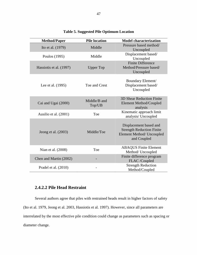
47
Table 5. Suggested Pile Optimum Location
Method/Paper Pile location Model characterization
Ito et al. (1979) Middle Pressure based method/
Uncoupled
Poulos (1995) Middle Displacement based/
Uncoupled
Hassiotis et al. (1997) Upper Top
Finite Difference
Method/Pressure based/
Uncoupled
Lee et al. (1995) Toe and Crest
Boundary Element/
Displacement based/
Uncoupled
Cai and Ugai (2000) Middle/B and
Top/UB
3D Shear Reduction Finite
Element Method/Coupled
analysis
Ausilio et al. (2001) Toe Kinematic approach limit
analysis/ Uncoupled
Jeong et al. (2003) Middle/Toe
Displacement based and
Strength Reduction Finite
Element Method/ Uncoupled
and Coupled
Nian et al. (2008) Toe ABAQUS Finite Element
Method/ Uncoupled
Chen and Martin (2002) - Finite difference program
FLAC /Coupled
Pradel et al. (2010) - Strength Reduction
Method/Coupled
2.4.2.2 Pile Head Restraint
Several authors agree that piles with restrained heads result in higher factors of safety
(Ito et al. 1979, Jeong et al. 2003, Hassiotis et al. 1997). However, since all parameters are
interrelated by the most effective pile condition could change as parameters such as spacing or
diameter change.
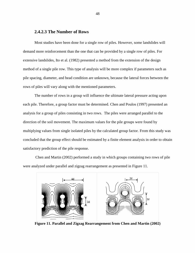
48
2.4.2.3 The Number of Rows
Most studies have been done for a single row of piles. However, some landslides will
demand more reinforcement than the one that can be provided by a single row of piles. For
extensive landslides, Ito et al. (1982) presented a method from the extension of the design
method of a single pile row. This type of analysis will be more complex if parameters such as
pile spacing, diameter, and head condition are unknown, because the lateral forces between the
rows of piles will vary along with the mentioned parameters.
The number of rows in a group will influence the ultimate lateral pressure acting upon
each pile. Therefore, a group factor must be determined. Chen and Poulos (1997) presented an
analysis for a group of piles consisting in two rows. The piles were arranged parallel to the
direction of the soil movement. The maximum values for the pile groups were found by
multiplying values from single isolated piles by the calculated group factor. From this study was
concluded that the group effect should be estimated by a finite element analysis in order to obtain
satisfactory prediction of the pile response.
Chen and Martin (2002) performed a study in which groups containing two rows of pile
were analyzed under parallel and zigzag rearrangement as presented in Figure 11.
Figure 11. Parallel and Zigzag Rearrangement from Chen and Martin (2002)

49
From the study, the parallel arrangement was found similar to the case for single row of
piles. While for the zigzag arrangement, was found to provide more resistance to soil movement
due to the multiple soil arching effects that can be developed by this type of arrangement. The
arching effect is considered a stabilizing mechanism that according to Chen and Martin (2002) is
limited by pile spacing. For drained conditions, the lateral forces on the pile are reduced with
reducing space. On the other hand, for the undrained conditions, the forces action on the pile will
be higher and the group effects can be considered not significant.
2.4.2.4 Pile Length and Embedment
This parameter will control the soil failure mode as mentioned before the intermediate
mode of failure will yield the maximum shear and bending moment resistance. Hence, an
adequate length of pile may be assured to achieve the required embedment. Poulos (1995)
suggested that the pile length must be increase if the critical failure surface is near or below the
pile tips. He suggested that the optimum depth at which the maximum resistance is developed
(hence, the intermediate mode of failure will develop) is when the failure surface is located at 0.6
to 0.75 times the length of the pile. In other words, the length of the pile in the stable soil must
be 0.4 to 0.35 times the length of the pile to ensure the optimum mode of failure. Therefore, pile
length depends on the characteristics of the analyzed slopes and will be different for each studied
case. The embedment depth has been suggested to be 0.5 the ratio sliding depth / pile length
which means at least half of the pile must be placed in the stable zone.

50
2.4.2.5 Type of Soil
The properties of the material within the slope will primarily define the characteristics of
the critical surface failure. For a soil with a large cohesion and a small friction angle, the most
critical failure surface will be a deep circle, while shallow circle will be the critical slide surface
for a soil with a small cohesion and a large friction angle material (Huang 2014, NAVFAC
(1986)). This is especially important for an uncoupled analysis where the slope stability analysis
is performed based on LEM in which assumptions regarding the shape and location of the failure
will be done. That assumption will consequently influence the lateral; response since pile
embedment, maximum moment and shear will varies regarding the surface failure depth.
2.4.3 Advantages and Disadvantages of LEM vs Numerical Modeling
This section is focused on the comparison between performing analysis by LEM, which
means an uncoupled analysis and performing geomechanical analyses (coupled approached). The
advantages and disadvantaged presented in Table 6 are summarized from the literature review
from several authors such as Duncan (1996), Geo-Slope International (2010), Cai and Ugai
(2000), Nian et al. (2008), Pradel and Chang (2011), Griffins and Lane (1999), Jeong et al.
(2003), Won et al. (2005). The uncoupled approach is separated into displacement and pressure-
based because different advantages and disadvantages from each method were found.

51
Table 6. Compassion LEM and Numerical Modeling
LEM-Pressure based LEM-Displacement
based Numerical modeling; FE/FDM
Advantages
Well known-widely applied
Considered of easy application
and simple.
Well known-widely
applied.
Considered of easy
application and simple.
Able to directly measure
accurate pile responses
from the soil movement.
Considered an
intermediate solution
between pressure-based
and FE/FD modeling.
A single analysis can be
performed.
No assumption of the location
and shape of the critical surface
failure.
Failure mechanism no need
assumption.
Sensitivity analysis to determine
different design alternatives can
be more easily done.
Progressive failure and shear
failure can be monitored.
Disadvantages
Soil-pile interaction is not
considered.
The method is considered
conservative.
The assumptions are considered
simplified.
Assumption regarding the
location and shape of the critical
surface failure is needed.
Considers a fixed critical surface
Does not consider pile flexibility,
saturation and arching of clays.
Considers the soil able to
plastically deform around the
pile. Thus, does not represent the
real soil/pile interaction.
Two analyses should be
performed (slope and pile).
Needs accurate values of
displacement to be
reliable.
Greatly depends on the
soil properties
representation for the
lateral analysis (p-y
curves).
Two analyses should be
performed (slope and
pile).
Complex and costly.
May required lab calibration.
Could require considerable time.
Knowledge is required to avoid
misuse and misinterpretation of
the results.
Highly dependent in the
constitutive model for soil.

52
2.4.4 Step-by-Step Design Approach for Pile Reinforced Slopes
After the selection of the general analysis as either uncoupled or coupled, step-by-step
procedures must be followed to ensure the correct application of the selected method of analysis.
For the uncoupled analysis several authors (Isenhower et al. 2016, Vessely et al. 2007,
Reese et al. 2004, Esser and Vanden Berge 2010, among others) suggested a procedure that can
be summarized as follows:
For Distributed Load Approach:
1. Determine if the slope requires reinforcement by performing an unreinforced analysis and
comparing the factor of safety to a target value.
2. Determine the require loads for stabilization that will reach the target factor of safety.
This must be determined by performing the stability analysis after placing the pile in the
proposed position. From the analysis the location of the critical surface should be also
determined.
3. Analyze the pile response with a computer program. In this study, LPILE will be used.
4. Develop p-y curves for the soil above and below the sliding mas (modifiers should be
applied for active landslide and closely-spaced shafts).
5. Applied a distributed load to the pile that could follow: (NAVFAC (1986), Reese et al.
(2004), ODOTO (2011). The distributed load must be applied from the ground surface to
the sliding depth.
6. Determine the pile responses to the applied loads and compare the maximum bending
moment and shear to the nominal values of the pile to verify structural integrity.
53
For Displacement-based Analysis:
1. Follow steps from 1 to 4 from the previous method.
2. Defined a soil movement profile along the length of the pile, the soil movement must be
evaluated before (From in situ measurements, finite element analysis, correlation with
case studies).
3. Determined the pile responses to the applied soil movements and follow step 6 for
distributed load approach.
For Coupled Analysis:
For the coupled analyses, the soil properties and constitutive model must be selected. The
slope and the pile are modeled together, thus, the most important key to the accuracy of the
results is the correct representation of the materials and conditions that will be modeled. As
in the uncoupled analysis, it must be determined if the slope requires reinforcement by
performing an unreinforced analysis. Furthermore, if the reinforcement is required the pile
must be placed at the proposed position and the new factor of safety could be evaluated.
From the analysis, the maximum bending and shear in the pile should be compared with the
nominal values of the pile to verify structural integrity.
For both coupled and uncoupled if the structural integrity of the pile is compromised
modifications on reinforcement, geometry or pile material must be done. Additionally, before
conducting the lateral response analysis it must be established if the loads from the slope
stability analysis correspond to factored or unfactored loads to relate them to LRFD or ASD
analysis. Currently, for the displacement-based method, the analysis can only be conducted
for ASD; it must be specified if the value used for the pile analysis is ultimate or allowable.
54
CHAPTER 3. STUDIED PROBLEMS
3.1 General Information
In this chapter, three cases will be analyzed. Each of the cases will represent a different
soil or reinforcement condition. The cases are studies previously presented by other authors with
the objective of verifying, validating, or contrasting the results. For each case, description, soil
properties, and results will be presented. Regarding the analyses, the unreinforced condition will
be analyzed first followed by the reinforced condition. Moreover, limit equilibrium followed by
finite element analyses will be presented following a general classification as uncoupled (limit
equilibrium-pile analysis) and coupled (FD and FE analysis).
As stated previously, the analyses will be performed by two limit equilibrium based
programs (Slope W and Slide 7.0) in conjunction with LPILE for the analysis of the laterally
loaded pile followed by a 2D finite difference analysis using FLAC and the 2-dimensional
elasto-plastic finite element analysis by the shear strength reduction method using Phase2. In this
thesis, for the limit equilibrium analyses, the procedure presented by Poulos (1995) will be
followed. The unreinforced analysis will be performed, then the shear force necessary to achieve
a minimum factor of safety depending on the target value for each case will be determined.
The required stabilizing force will be used for verification in a new stability analysis and
finally, the resistance developed by the piles will be verified to guarantee that the pile will
provide the necessary force. The overall results will be summarized and discussed for each
specific case in the following chapters.

55
3.2 Problem I: Layered Frictional Case
A layered slope consisted mainly of frictional materials will be studied. Figure 12
presents the general geometry of the slope. This corresponds to chainage 3225, western side,
state highway 23, Newcastle, Australia presented by Poulos (1995). The soil properties of the
slope are presented in Table 7. In this case, constructability issues resulted in the creation of
slopes up to 8m. Hence, the stability analyses were conducted to verify the areas considered
unstable and installation of pile as reinforcement was suggested.
Figure 12. Geometry Probem I
The stability analysis will be performed by following the original assumptions presented
by Poulos (1995); a circular slip surface and using the Bishop’s simplified method. It is
important to highlight that the circular assumption is just necessary for the limit equilibrium
analysis. The existence of a weak stratum within the geometric configuration of the slope is the
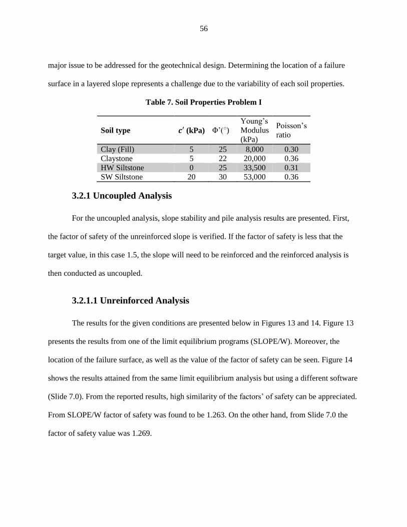
56
major issue to be addressed for the geotechnical design. Determining the location of a failure
surface in a layered slope represents a challenge due to the variability of each soil properties.
Table 7. Soil Properties Problem I
Soil type 𝒄′ (kPa) Φ’()
Young’s
Modulus
(kPa)
Poisson’s
ratio
Clay (Fill) 5 25 8,000 0.30
Claystone 5 22 20,000 0.36
HW Siltstone 0 25 33,500 0.31
SW Siltstone 20 30 53,000 0.36
3.2.1 Uncoupled Analysis
For the uncoupled analysis, slope stability and pile analysis results are presented. First,
the factor of safety of the unreinforced slope is verified. If the factor of safety is less that the
target value, in this case 1.5, the slope will need to be reinforced and the reinforced analysis is
then conducted as uncoupled.
3.2.1.1 Unreinforced Analysis
The results for the given conditions are presented below in Figures 13 and 14. Figure 13
presents the results from one of the limit equilibrium programs (SLOPE/W). Moreover, the
location of the failure surface, as well as the value of the factor of safety can be seen. Figure 14
shows the results attained from the same limit equilibrium analysis but using a different software
(Slide 7.0). From the reported results, high similarity of the factors’ of safety can be appreciated.
From SLOPE/W factor of safety was found to be 1.263. On the other hand, from Slide 7.0 the
factor of safety value was 1.269.

57
Figure 13. Unreinforced SLOPE/W
Figure 14. Unreinforced Slide 7.0
58
3.2.1.2 Reinforced Analysis
Reinforced analyses were conducted by placing a pile near the mid-slope. They are two
(2) methods to determine the required shear force from a reinforcement to achieve the target
factor of safety: (1) “Method A” and (2) “Method B” by Duncan and Wright (2005). In this
study, the “Method A” will be used to compare among programs. However, “Method B” will be
also used for comparison with the original case study that presumably employed the mentioned
method to determine the required shear.
The “Method A” has been selected because as suggested by Duncan and Wright (2005),
soil and reinforcement have different sources of uncertainties. Thus, it would be more accurate to
factor the forces separately as in “Method A”, where the reinforcement forces are included in the
denominator of the factor of safety equation. This means that reinforcement forces are not
divided by the slope stability factor of safety.
The parameters needed it to conduct this analysis in the limit equilibrium programs are:
the shear force (To be determined), pile length (9m), and pile spacing (3m) as given by Poulos
(1995). For the limit equilibrium analysis, after performing the unreinforced analysis the required
stabilizing force must be determined. This force can be calculated from the stability analysis as
the necessary force from the reinforcement to reach the minimum factor of safety specify.
In Poulos (1995) the stabilizing force was computed as 87.5kN (per unit width of soil).
However, in the present study, the stabilizing force varies among the software and the
assumptions regarding its inclination. An initially reinforced analysis was performed with the
value presented by Poulos (1995).Subsequently, adjustments were made until the target factor of
safety was reached.
59
From SLOPE/W the factors of safety were found to be 1.59 and 1.58 for a force
perpendicular to the reinforcement and parallel to the slip respectively. The same values were
found for the corresponding analysis in Slide 7.0.
Furthermore, the values of shear forces to achieve 1.500 for “Method A” were
determined. For SLOPE/W the target value was found with a 61kN/m shear force when the
inclination of the force was assumed perpendicular to the reinforcement, while a slightly slower
F.S. was found for the parallel case (F.S.=1.490). The same analysis carried out by Slide 7.0,
yielded a shear force of 60kN/m to reach the target factor of safety in the perpendicular case and
again smaller F.S. in the parallel condition (F.S.=1.490).
If the analysis is conducted by the “Method B”, the value of shear presented by Poulos
(1995) achieved a 1.499 factor of safety. From the equation presented in Poulos’s study, equation
(2), it could be understood that the method used to determine the reinforcement load was
“Method B”. Hence by indicating “Passive” method in Slide 7.0, the values of the required shear
from the present and previous study (87.5kN/m) produces very similar factors of safety.
Therefore, as indicated by the reviewed literature (Duncan and Wright 2005), the “Method B” is
more conservative than the “ Method A” demanding higher shear from the reinforcement to
achieve same factor of safety since the force is divided by the slope factor of safety.
Table 8 presents a summary of the factors of safety from the reinforced limit equilibrium
analysis. Figure 15 presents pile location, critical surface, and target factor of safety for the
general case and also a comparison between the reinforced and unreinforced critical surface’s
location.

60
Table 8. Factors of Safety Reinforced Limit Equilibrium Analyses
Method
Required
Shear
(kn/m)
Perpendicular to
the pile
Parallel to the
slip
Method A
(Allowable)
kN/m SLOPE/W Slide
7.0 SLOPE/W
Slide
7.0
87.5 1.590 1.590 1.580 1.580
60 - 1.500 1.490
61 1.500 - 1.490 -
Original
Poulos * 87.5 1.500
Method B - 1.499 - 1.494
*Poulos (1995) stability analysis was not performed with SLOPE/W or Slide 7.0.
Figure 15. Unreinforced (F=1.269) and Reinforced (F=1.499) Results Problem I
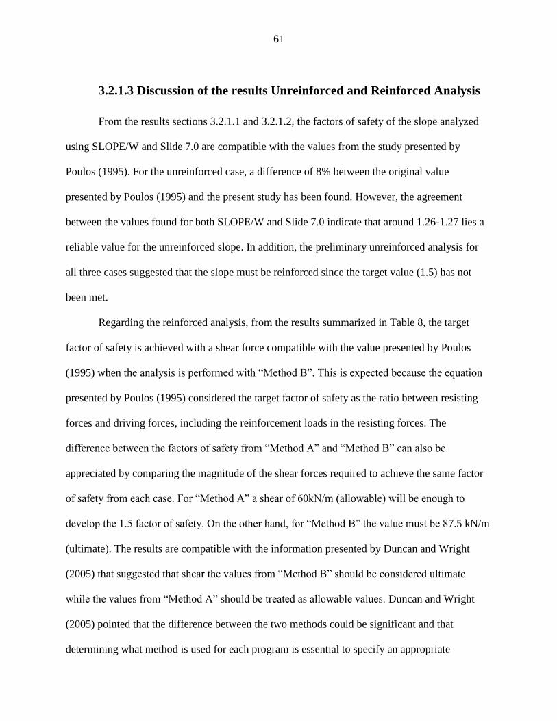
61
3.2.1.3 Discussion of the results Unreinforced and Reinforced Analysis
From the results sections 3.2.1.1 and 3.2.1.2, the factors of safety of the slope analyzed
using SLOPE/W and Slide 7.0 are compatible with the values from the study presented by
Poulos (1995). For the unreinforced case, a difference of 8% between the original value
presented by Poulos (1995) and the present study has been found. However, the agreement
between the values found for both SLOPE/W and Slide 7.0 indicate that around 1.26-1.27 lies a
reliable value for the unreinforced slope. In addition, the preliminary unreinforced analysis for
all three cases suggested that the slope must be reinforced since the target value (1.5) has not
been met.
Regarding the reinforced analysis, from the results summarized in Table 8, the target
factor of safety is achieved with a shear force compatible with the value presented by Poulos
(1995) when the analysis is performed with “Method B”. This is expected because the equation
presented by Poulos (1995) considered the target factor of safety as the ratio between resisting
forces and driving forces, including the reinforcement loads in the resisting forces. The
difference between the factors of safety from “Method A” and “Method B” can also be
appreciated by comparing the magnitude of the shear forces required to achieve the same factor
of safety from each case. For “Method A” a shear of 60kN/m (allowable) will be enough to
develop the 1.5 factor of safety. On the other hand, for “Method B” the value must be 87.5 kN/m
(ultimate). The results are compatible with the information presented by Duncan and Wright
(2005) that suggested that shear the values from “Method B” should be considered ultimate
while the values from “Method A” should be treated as allowable values. Duncan and Wright
(2005) pointed that the difference between the two methods could be significant and that
determining what method is used for each program is essential to specify an appropriate
62
reinforcing force. The results also suggest that assuming the inclination of the shear forces either
perpendicular to the reinforcement or parallel to the critical surface does not represent
significance source of variability among the results. For this case, the variability regarding the
mentioned assumption does not represent more than 1%.
Figure 15 shows the changes on the critical failure position when the reinforcement have
been placed as indicated by several authors from the literature review (Ausilio et al. 2001, Ito
and Matsui 1975, Lee et al. 1995). Therefore, when assuming a fixed location of the sliding
surface the actual soil/pile interaction mechanism is not accurately represented. The sliding
depth is an important factor to determine the structural integrity of the laterally loaded pile. The
difference between the presented results in terms of the required shear for the target factor of
safety among methods is graphically presented in Figure 16.
Figure 16. Shear Force to Achieve F.S.=1.5 among Methods
0
20
40
60
80
100
Method A Method B Original Poulos
*
Shea
r (k
N/m
)
Analysis Method

63
3.2.1.4 Sensitivity Analyses (Uncoupled)
After the stabilizing force has been determined, additional analysis were performed with
the calibrated condition that matches Poulos (1995). The purpose of this analysis is to study the
influence of pile length in the required reinforcing load to achieve the target factor of safety. In
some cases, the values of the target factor of safety were not achieved no matter the magnitude of
the shear. For those cases, the optimum value at which the factor of safety did not present any
improvement has been specified. Table 9 summarizes the results from the mentioned analyses.
Table 9. Pile Lenght Influence on Required Shear Force
Length
of Pile
(L1, m)
Critical
surface
depth
(L2,m)
**L2/L1
Required
shear
(kN/m)
F.S.
achieved
Ratio
Length/Shear
6* 6 1.02 >48 1.33 -
7* 7.2 1.00 >46.6 1.42 -
8* 8.09 1.01 >85 1.491 -
9 5.4 0.60 90 1.5 10%
12 5.4 0.45 90 1.5 13%
14 5.4 0.38 90 1.5 16%
18 5.4 0.30 89 1.5 20%
*Not 1.5 could be achieved.
**L2/L1, ratio sliding surface/ pile length
From the results presented by Table 9, there is an optimal length at which the required
shear could be minimized to achieve the target value, 9.0m. For relatively short piles (piles
considered not to be embedded on the firm strata, less than 0.6 in this case) the target factor of
safety was not reached. These piles represented critical surfaces touching the pile tip. After the
pile length is increased beyond the optimum length, the required shear was not decreased. The
ratio length/shear represents the relationship in percentages of shear by length to achieve the
indicated factor of safety. Thus, piles having between 8.0m and 9.0m will represent the most
efficient alternative since 1.491 could be acceptable if the target F.S.=1.5. Piles having 8m will

64
have a failure surface below the pile tip which indicates that the failure surface has been forced
below the reinforcement in this case with an acceptable factor of safety.
Moreover, to verify the influence of pile location within the slope into the factor of safety
a similar analysis was conducted placing piles with different lengths and same required shear
from the previous analysis, at different locations from the toe to the top of the slope. The results
are presented in Figure 17.
Figure 17. Factor of Safety vs Pile Location
For all piles (different length, same shear force), the highest factor of safety is found
when the pile is located in the middle of the slope (5.3m). The lowest factor of safety is found
when the pile is placed in the toe of the slope. After the optimum length has been achieved,
increasing length will not help to increase the factor of safety for the same shear force. Piles
located around the top seem to be another good alternative for the configuration of this slope.
However, as the distance from the toe increases, the length of the pile may also be increased to
1.2
1.25
1.3
1.35
1.4
1.45
1.5
1.55
0 2 4 6 8 10 12
F.S
.
Distance from the Toe (m)
Pile 8m, 87.5kN Pile 9m, 87.5kN Pile 12m, 87.5kN
Unreinforced
F.S.
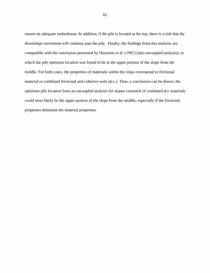
65
ensure an adequate embedment. In addition, if the pile is located at the top, there is a risk that the
downslope movement will continue past the pile. Finally, the findings from this analysis are
compatible with the conclusion presented by Hassiotis et al. (1997) (also uncoupled analysis), in
which the pile optimum location was found to be at the upper portion of the slope from the
middle. For both cases, the properties of materials within the slope correspond to frictional
material or combined frictional and cohesive soils (ϕ-c.). Thus, a conclusion can be drawn, the
optimum pile location from an uncoupled analysis for slopes consisted of combined ϕ-c materials
could most likely be the upper portion of the slope from the middle, especially if the frictional
properties dominate the material properties.

66
3.2.1.5 Designing Resisting Pile
After the target factor of safety has been achieved, the pile analysis must be conducted to
ensure that the piles will develop the required resistance. In the original analysis, Poulos (1995)
used a simplified boundary element program in which the soil was modeled as an elastic
continuum and the pile as a simple elastic beam. In this study, since LPILE will be used, the
basics of the analysis (p-y model for soil) consider the soil as a series of discrete resistances and
the pile as non-linear and elastic beam.
From the stability analisys, the sliding surface will be taken to be at 5.4m below the pile
top. Hence, the moving soil will consist on the claystone, while the stable soil will be the slightly
and the highly weathered siltstone, as presented in Figure 18.
Figure 18. Critical Circle after Stabilization
67
The parameters used for the analysis are presented in Table 10. The soil properties
presented by Poulos (1995) will be used and correlated when needed, to develop the p-y curves
as user defined, following the procedure presented by Reese et al. (2004) and Isenhower et al.
(2016). To generate the p-y curves for the weathered rocks, the stiff clay model has been used as
presented by Gabr et al. (2002)for a possible approach for the generation of p-y curves in
weathered rocks (following from Reese et al. (1975)).
The p-y curves for this problem are presented in Figure 19. Since the top of the pile is
located on the mid-slope, the first curve for the analysis will be for the claystone strata. The
maximum moment capacity for the section was found to be 3,393kN-m unfactored. This value is
compatible with the value presented by Poulos (1995), approximately 3,100kN-m.
Table 10. Summary of Parameters for Pile Lateral Analysis
Pile diameter (Bored
concrete pile) 1.2m
Reinforcement
equivalent area 2.5% of Ac
Yield stress of
reinforcement 260Mpa
Young’s modulus of the
soil
Varying from 5Mpa at a rate
of 3Mpa/m
Unstable soil limiting
lateral pressure
As presented by (Reese et al.
2004)
Stable soil limiting
lateral pressure
4xHorizontal earth
coefficient

68
Figure 19. p-y cuves for Laterally Loaded Pile Analysis
To perform the displacement-based method, the best way to estimate the lateral soil
movement as indicated by Jeong et al. (2003) is from reliable in situ measurements. However,
approximation of the movement can be done by correlations or using finite element programs,
when field test data is not available. In this study, the displacement used comes from the
computations in FLAC.
Because the spacing between the piles is 3m (less than 3.5 diameters), modification
should be applied to the soil resistance. Reese et al. (2007) suggested that for a single row of pile
placed side by side, the p-modifier should be calculated as:
𝛽2 = 0.64 (𝑆
𝐷)0.34
Where 𝛽2 is the modifier for soil resistance, S is spacing and D pile diameter. In the
present case 𝛽2 = 0.87.
0
50
100
150
200
250
300
0 0.2 0.4 0.6 0.8 1 1.2
Soil
Forc
e, k
N/m
Pile deflection, m
Claystone
HW Siltstone
SW Siltstone
(11)

69
An additional analysis will be conducted, for this analysis, the shear force from the LE
analyses will be applied to the pile as a distributed load. The analysis follows the procedure
presented by The Ohio Department of Transportation (ODOTO 2011). Figure 20 presents the
distribution of the lateral load on the pile. In this analysis, because the results from FLAC and
Phase2 do not factor the shear force by the slope stability factor of safety, the required shear will
be considered allowable and the value from “Mathod A” will be used as unfactored load.
Figure 20. Distribution of Lateral Load on a Pile as Suggested by ODOTO (2011)
Where;
Fh is the lateral load per unit length of embankment required by slope stability analysis, s
is center-to-center pile spacing, r is number of rows of piles, l is distance from ground surface to
failure plane, P is distributed lateral load at the failure h plane for use in lateral pile analyses.
The distributed load is presented in Table 11.
The results from the lateral analysis are presented in Figure 21. It should be pointed that
the results from the displacement-based analysis greatly depend on the input displacements, for
small soil movements smaller stabilizing forces will be achieved.

70
Displacement-based Method*Unfactored values
Distributed Load Method* Unfactored values
Figure 21. Bending Moment and Shear from Lateral Response Analyses

71
Table 11. Distribution of Lateral Loads for Pile Design Problem I
Variable Value
Fh 61kN (per width of soil, Unfactored)
s 3m
r 1 rows
l 5.4m
Ph 61kN/m per pile
From Figure 21, the results from the displacement-based approach and the ones applying
a uniform load from the stability analysis to the pile are similar. The maximum values for both
conditions are located around the same depth. The summary of the results is presented in Table
12. To verify the pile structural integrity, the results are compared to the nominal ultimate
bending moment and shear for the reinforced concrete section. The factors of safety should be
>1.67 for flexure and >1.5 for shear. The shear at the sliding depth for this case does not
correspond to the maximum shear. Thus, to verify the structural integrity the maximum shear
should be compared with the factored shear resistance of the pile no matter the location.
Table 12. Lateral Analisys Results (Unfactored loads)
Parameter Distributed load
approach
Displacement based (90mm)
Unfactored
nominal capacity
of pile
3,393 kN.m 3,393 kN.m
Maximum
applied moment 306 kN.m 237 kN.m
Unfactored
resisting shear
force
1018 kN 1018 kN
Maximum shear
force at critical
circle
138 kN 87 kN

72
3.2.2 Coupled Analysis
For this analysis, the unreinforced analysis will also be performed to verify if the target
factor of safety is reached (as presented in section 3.2.1.1). The reinforced analysis will then be
conducted after placing the reinforcing pile.
3.2.2.1 Unreinforced Analysis
The unreinforced factor of safety for this condition has been determined from the 2-D
elasto-plastic finite element analysis by the shear strength reduction method using Phase2.
Additional results are also presented from the analysis in the finite difference program FLAC.
The factor of safety is calculated using the Shear Strength Reduction method (SSR). To
represent the soil behavior the Mohr-Coulomb failure criterion has been selected. This is because
this criterion has been found simple and accurate in representing the soil behavior. In addition,
its parameters has physical meaning and it is generally accepted in the geotechnical area (Labuz
and Zang 2012).
Figure 22 presents the results from the FE SSR analysis performed using Phase2. The
contours of maximum solid displacement at failure computed by the SSR method with the LE
critical failure circle superposition shows a good agreement. Table 11 shows a summary for a
general comparison of the unreinforced analyses from LE, FE and FD programs.
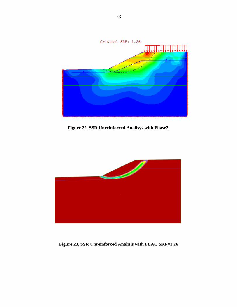
73
Figure 22. SSR Unreinforced Analisys with Phase2.
Figure 23. SSR Unreinforced Analisis with FLAC SRF=1.26

74
Table 13. Summary Unreinforced Analyses Problem I
Programs SLOPE/W Slide 7.0 Phase2 FLAC
Unreinforced F.S. 1.263 1.269 1.260 1.26
The summary from the unreinforced analysis clearly indicates that results from LE
analyses can be reproduced by SSR FE and FD analyses with high agreement. In this case,
layered slope with different soil properties, the difference among results is less than 1%, thus all
methods are relatively accurate and reliable.
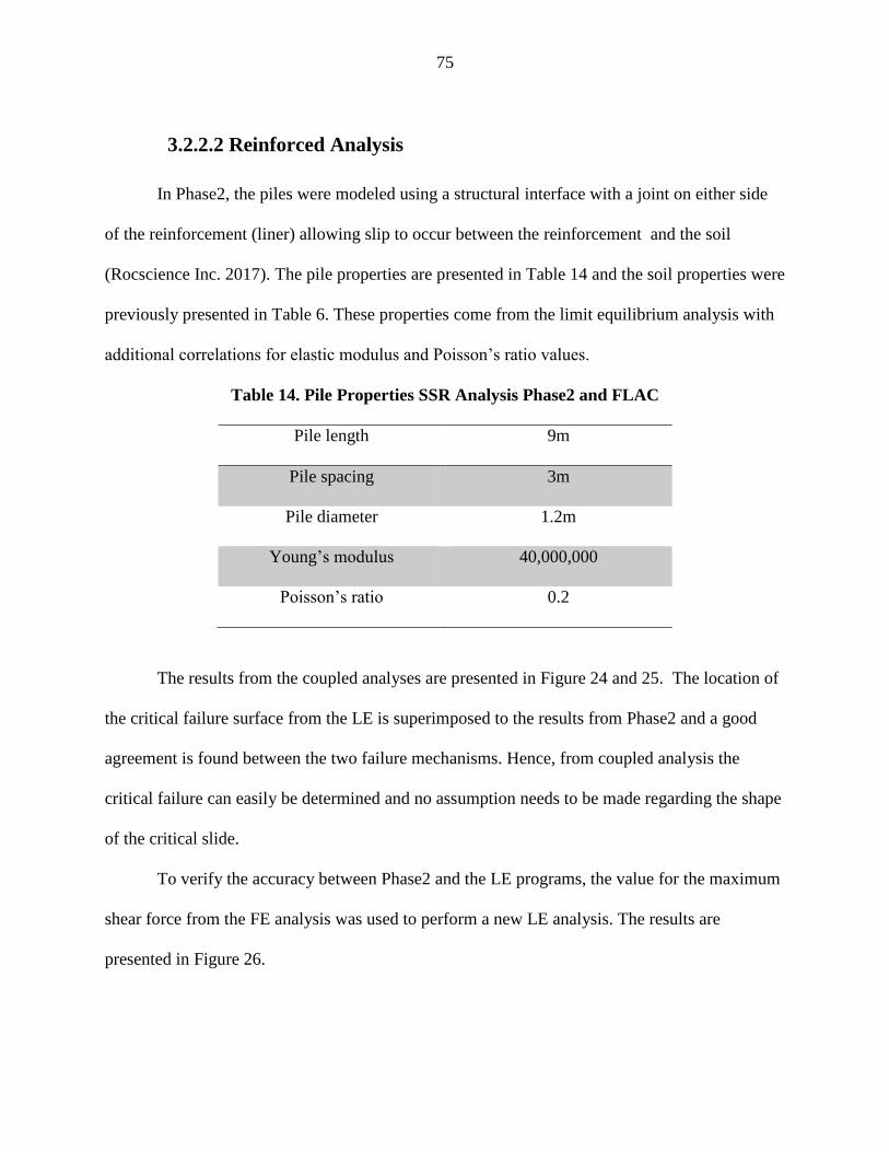
75
3.2.2.2 Reinforced Analysis
In Phase2, the piles were modeled using a structural interface with a joint on either side
of the reinforcement (liner) allowing slip to occur between the reinforcement and the soil
(Rocscience Inc. 2017). The pile properties are presented in Table 14 and the soil properties were
previously presented in Table 6. These properties come from the limit equilibrium analysis with
additional correlations for elastic modulus and Poisson’s ratio values.
Table 14. Pile Properties SSR Analysis Phase2 and FLAC
Pile length 9m
Pile spacing 3m
Pile diameter 1.2m
Young’s modulus 40,000,000
Poisson’s ratio 0.2
The results from the coupled analyses are presented in Figure 24 and 25. The location of
the critical failure surface from the LE is superimposed to the results from Phase2 and a good
agreement is found between the two failure mechanisms. Hence, from coupled analysis the
critical failure can easily be determined and no assumption needs to be made regarding the shape
of the critical slide.
To verify the accuracy between Phase2 and the LE programs, the value for the maximum
shear force from the FE analysis was used to perform a new LE analysis. The results are
presented in Figure 26.

76
Figure 24. SSR Reinforced Analisys with Phase2
Figure 25. SSR Reinforced Analisys with FLAC (FS=1.37)

77
Figure 26. Factor of Safety from Slide 7.0 for Shear Force from Phase2
From the results, for the same shear force both methods LE (Slide 7.0) and FE (Phase2)
produced very similar factors of safety, 1.392 From Slide 7.0 versus 1.38 from Phase2. This
indicates that if both analysis result in very similar factor of safety for the same shear, then from
the FE analysis, the shear resistance developed by the reinforcement under the analyzed
configuration (9m, location and diameter), is not enough to attain the target factor of safety.
From the reinforced analysis, section 3.2.2.2 the shear necessary to achieve 1.5 for a 9m long
pile was found to be 61kN (allowable and 87.5kN, ultimate). However, from this analysis
(coupled) the distribution of forces around the reinforcement indicates that modification in pile
geometry (length, diameter), pile location within the slope, or pile reinforcement is needed to
increase the shear resistance for achieving the desirable factor of safety.

78
3.2.2.3 Sensitivity Analyses (Coupled)
To verify the influence of pile location within the slope into the factor of safety, a similar
analysis to that described in section 3.2.1.4 was performed in Phase2. Piles with different lengths
were placing at different locations from the toe to the top of the slope. The results are presented
in Figure 27.
Figure 27. Factor of Safety vs Pile Location Original Condition
From a coupled analysis as presented before by Jeong et al. (2003), Won et al. (2005),and
Cai and Ugai (2000), the optimum pile location from SSR FE analysis was reported to be in the
middle of the slope. However, from Figure 27, in this case, the optimum location is found at a
distance Le/4 (quarter of the slope from the toe) for the smaller piles. As the pile length
increases, the optimum location changes to the middle of the slope. Comparing the results from
Sections 3.2.1.4 and 3.2.2.3, the results suggest that from uncoupled analysis the pile optimum
location is in the middle and around the top as presented by Hassiotis et al. (1997). On the other
1.2
1.3
1.4
1.5
1.6
1.7
1.8
1.9
0 2 4 6 8 10 12
F.S
.
Distance from the Toe (m)
Pile 8m Pile 9m Pile 12m
Unreinforced
F.S.

79
hand, for the same slope, the coupled analysis suggested to place the pile around middle being
slightly higher the factor of safety of the piles located around the quarter of the slope (for shorter
piles). Hence, the common findings among methods for the properties of the material of this
slope (frictional) are: piles located at the toe do not represent a favorable condition, and placing
piles around the middle will always increase the factor of safety especially when an adequate
embedment depth is assured.
Figure 28. Optimun Location Coupled and Uncoupled Analyses
1.2
1.3
1.4
1.5
1.6
1.7
1.8
0 2 4 6 8 10 12
F.S
.
Distance from the Toe (m))
Pile 8m-Uncoupled Pile 9m-Uncoupled
Pile 12m-Uncoupled Pile 8-Coupled
Pile 9m-Coupled Pile 12m-Coupled
Unreinforced
F.S.
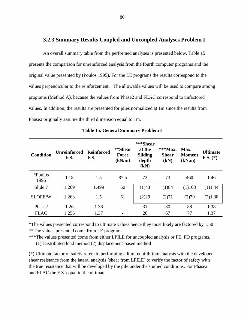
80
3.2.3 Summary Results Coupled and Uncoupled Analyses Problem I
An overall summary table from the performed analyses is presented below. Table 15
presents the comparison for unreinforced analysis from the fourth computer programs and the
original value presented by (Poulos 1995). For the LE programs the results correspond to the
values perpendicular to the reinforcement. The allowable values will be used to compare among
programs (Method A), because the values from Phase2 and FLAC correspond to unfactored
values. In addition, the results are presented for piles normalized at 1m since the results from
Phase2 originally assume the third dimension equal to 1m.
Table 15. General Summary Problem I
Condition Unreinforced
F.S.
Reinforced
F.S.
**Shear
Force
(kN/m)
***Shear
at the
Sliding
depth
(kN)
***Max.
Shear
(kN)
Max.
Moment
(kN.m)
Ultimate
F.S. (*)
*Poulos
1995 1.18 1.5 87.5 73 73 460 1.46
Slide 7 1.269 1.499 60 (1)43 (1)84 (1)103 (1)1.44
SLOPE/W 1.263 1.5 61 (2)29 (2)71 (2)79 (2)1.38
Phase2 1.26 1.38 - 31 80 88 1.38
FLAC 1.256 1.37 - 28 67 77 1.37
*The values presented correspond to ultimate values hence they most likely are factored by 1.50
**The values presented come from LE programs
***The values presented come from either LPILE for uncoupled analysis or FE, FD programs.
(1) Distributed load method (2) displacement-based method
(*) Ultimate factor of safety refers to performing a limit equilibrium analysis with the developed
shear resistance from the lateral analysis (shear from LPILE) to verify the factor of safety with
the true resistance that will be developed by the pile under the studied conditions. For Phase2
and FLAC the F.S. equal to the ultimate.

81
For the unreinforced analyses, all methods of analysis achieve around the same factor of
safety. Thus, LE, FE, or FD programs are comparatively recommended regarding accuracy and
reliability.
For the reinforced analyses, to compare the results from coupled and uncoupled analysis,
the shear resistance developed by the pile and the factor of safety can be compared. On one hand,
the shear resistances from LPILE (for uncoupled condition) are similar to the values from the
Phase2 and FLAC. This indicates that the ultimate factor of safety of an uncoupled analysis will
be lower than the target factor since the resistance of the pile will not be developed a hundred
percent (as in a superposition case where the applied load will be equal to the resistance). Hence,
results strongly indicate that coupled analyses are able to predict a more realistic force
distribution along the reinforcement (for the uncouple analyses, the user is able to manually
insert different shear without taking into account pile properties or whether or not the selected
pile will develop the necessary shear).
For the displacement-based method (2), the prediction of the factor of safety was found to
be similar to the results from the coupled analysis performed by FLAC. For the same
displacement (90mm from FLAC analysis), the displacement-based analysis from LPILE yields
slightly higher values for both bending moment and shear resistance. The values from the
distributed load approach, on the other hand, where found higher for all parameters. The findings
are consistent with the one described by Jeong et al. (2003) and Won et al. (2005), indicating that
the displacement-based method is intermediate in theoretical accuracy between the coupled
analysis and the uncoupled analysis (based in distributed load and Bishop’s method), being the
results from an uncoupled analysis more conservative.

82
Overall, the ultimate factors of safety are similar. Thus, performing a coupled or
uncoupled pile reinforced slope analysis will yield similar results. Then, it should be questioned
if the degree of effort from performing two separate analyses (slope and pile) for uncoupled
condition is indeed smaller than the degree of effort for the inputs parameters needed to perform
a coupled analysis. On one hand, to perform an uncoupled analysis, assumptions regarding the
soil representation need to be made in order to developed the p-y curves, for combined ϕ-c
materials (silt like soil) and weathered rocks equivalent models should be used since no widely
known model to developed p-y curves for materials having friction and cohesion has been
published (Gabr et al. 2002).
In addition, duality of the factors (geotechnical factor of safety and structural factor of
safety) is most likely to occur if the balance and unbalance forces are not clearly defined.
Moreover, as mention previously, assuming the pile will reach a desired shear without taking pile
properties into account (just equilibrium) does not represent the real soil/structure interaction.
Also, iterations will be needed to match pile resistance, slip surface and pile stiffness for some of
the original uncouple approaches (Pradel et al. 2010).
In contrast, to perform the coupled analysis, the effort just needs to be focused on
determining the required parameters for the model. The coupled analysis requires considerably
more parameters that a limit equilibrium one. However, no assumptions on failure mechanism,
empirical models (p-y curves), or modifiers will be needed. Additional parameters can be seen as
a better way to represent the soil instead of an increasing in input effort.
Regarding the lateral analysis (this is for both coupled and uncoupled), the pile structural
integrity is verified by comparing the maximum values to the nominal ones. In this case, to
compare among programs, the lateral analysis was performed with the unfactored loads from the
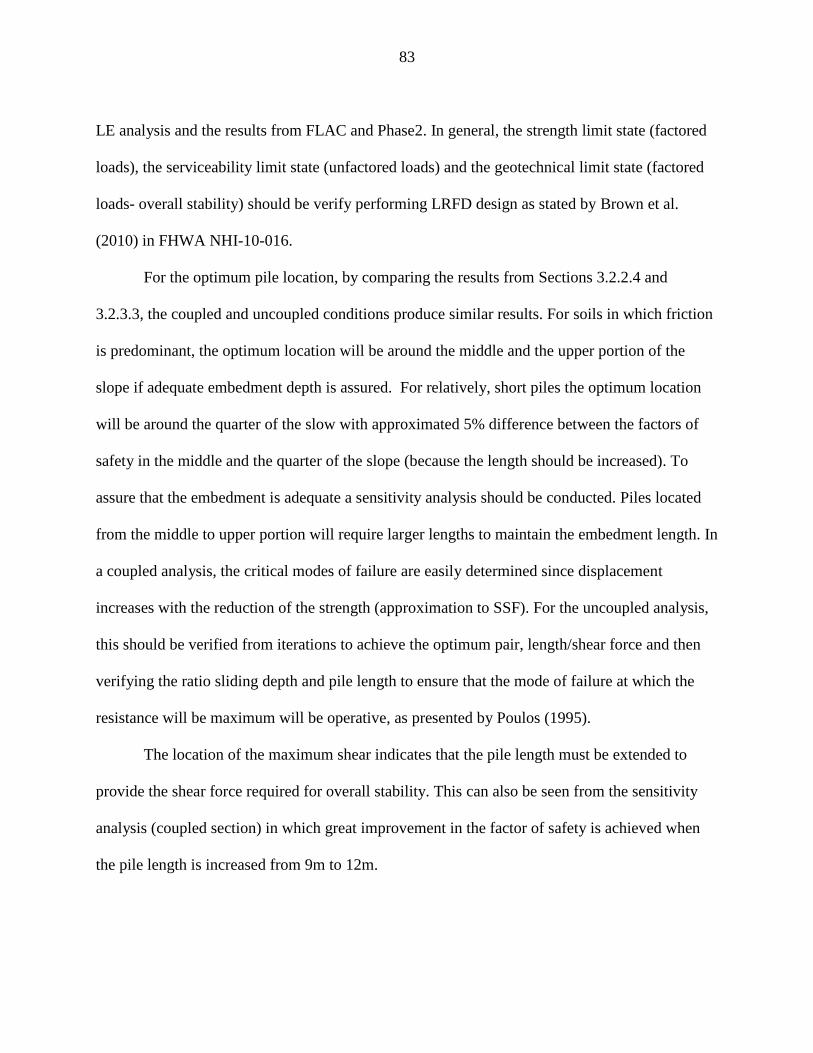
83
LE analysis and the results from FLAC and Phase2. In general, the strength limit state (factored
loads), the serviceability limit state (unfactored loads) and the geotechnical limit state (factored
loads- overall stability) should be verify performing LRFD design as stated by Brown et al.
(2010) in FHWA NHI-10-016.
For the optimum pile location, by comparing the results from Sections 3.2.2.4 and
3.2.3.3, the coupled and uncoupled conditions produce similar results. For soils in which friction
is predominant, the optimum location will be around the middle and the upper portion of the
slope if adequate embedment depth is assured. For relatively, short piles the optimum location
will be around the quarter of the slow with approximated 5% difference between the factors of
safety in the middle and the quarter of the slope (because the length should be increased). To
assure that the embedment is adequate a sensitivity analysis should be conducted. Piles located
from the middle to upper portion will require larger lengths to maintain the embedment length. In
a coupled analysis, the critical modes of failure are easily determined since displacement
increases with the reduction of the strength (approximation to SSF). For the uncoupled analysis,
this should be verified from iterations to achieve the optimum pair, length/shear force and then
verifying the ratio sliding depth and pile length to ensure that the mode of failure at which the
resistance will be maximum will be operative, as presented by Poulos (1995).
The location of the maximum shear indicates that the pile length must be extended to
provide the shear force required for overall stability. This can also be seen from the sensitivity
analysis (coupled section) in which great improvement in the factor of safety is achieved when
the pile length is increased from 9m to 12m.

84
3.3 Problem II –Homogeneous Cohesive Slope
A slope consisting of a uniform soil strata is presented in Figure 29. This correspond to a
generic case presented by the Dept. of the Navy, Naval Facilities Engineering Command,
NAVFAC (1986) to evaluate the influence of the reinforcement location in the value of the
factor of safety. The soil properties are presented in Table 16.
Figure 29. Geometry Probem II
The angle of inclination of the slope was determined to be 30 degrees. The final angle
used to evaluate the reinforced case was the inclination at which the unreinforced factor of safety
was found < 1.40 as suggested by Dept. of the Navy, Naval Facilities Engineering Command in
NAVFAC (1986) the publication.

85
Table 16. Soil Properties Problem II.
Soil type
Unit
Weight
(pcf) 𝒄′ (psf) Φ’()
Young’s
Modulus
(psf)
Υ
Clay (Fill) 114.38 200 17 208,854 0.3
Clay 112.40 200 15 208,854 0.4
3.3.1 Uncoupled analysis
For the uncoupled analysis, slope stability and pile analysis are presented. First, the factor
of safety of the unreinforced slope is verified. If the factor of safety is less than 1.4 the slope will
need to be reinforced and the reinforced analysis is conducted as uncoupled. Two different
conditions will be verified for this case (1) the factor of safety will be determined by assuming
the location of the slip surface, and (2) a general analysis will be conducted without restricting
the location of the failure surface.
3.3.1.1 Unreinforced Analysis
For the first condition, the failure surface will be constrained to an approximated value.
The failure surface according to NAVFAC (1986) would be around 9ft below the ground
surface. The factors of safety for this condition were found to be 1.354 and 1.357 in SLOPE/W
and Slide 7, respectively, as shown in Figures 30 and 31. Since both factors of safety were found
<1.40, the slope must be reinforced.
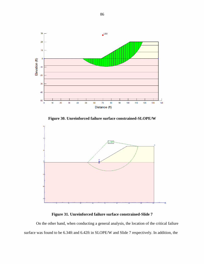
86
Figure 30. Unreinforced failure surface constrained-SLOPE/W
Figure 31. Unreinforced failure surface constrained-Slide 7
On the other hand, when conducting a general analysis, the location of the critical failure
surface was found to be 6.34ft and 6.42ft in SLOPE/W and Slide 7 respectively. In addition, the

87
factors of safety were found to be 1.316and 1.311 in SLOPE/W and Slide 7, respectively. Results
are presented in Figure 32 and 33.
Figure 32. Unreinforced unconstrained –SLOPE/W
Figure 33. Unreinforced unconstrained-Slide 7.0
For the unconstrained condition, reinforcement of the slope will also be needed. Table 17
summarizes the results from the unreinforced analyses for conditions one and two as presented

88
above. The results support the reviews from the literature that if the failure surface is assumed in
a fixed position, the results will be inaccurate. However, if the assumption is carefully done the
variation among the results could be minimized, at least for the unreinforced case.
Table 17. Summary Unreinforced Factors of Safety
Condition Critical surface
depth (ft) F.S.
Constrained
(SLOPE/W)
9.10
1.354
Constrained
(Slide 7) 1.357
Unconstrained
(SLOPE/W) 6.34 1.316
Unconstrained
(Slide 7) 6.42 1.311
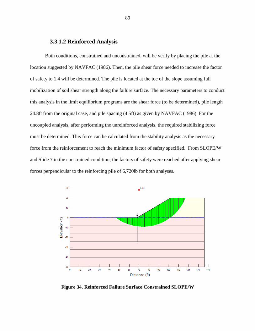
89
3.3.1.2 Reinforced Analysis
Both conditions, constrained and unconstrained, will be verify by placing the pile at the
location suggested by NAVFAC (1986). Then, the pile shear force needed to increase the factor
of safety to 1.4 will be determined. The pile is located at the toe of the slope assuming full
mobilization of soil shear strength along the failure surface. The necessary parameters to conduct
this analysis in the limit equilibrium programs are the shear force (to be determined), pile length
24.8ft from the original case, and pile spacing (4.5ft) as given by NAVFAC (1986). For the
uncoupled analysis, after performing the unreinforced analysis, the required stabilizing force
must be determined. This force can be calculated from the stability analysis as the necessary
force from the reinforcement to reach the minimum factor of safety specified. From SLOPE/W
and Slide 7 in the constrained condition, the factors of safety were reached after applying shear
forces perpendicular to the reinforcing pile of 6,720lb for both analyses.
Figure 34. Reinforced Failure Surface Constrained SLOPE/W

90
Figure 35. Reinforced Failure Surface Constrained Slide 7
On the other hand, when performing the unconstrained analyses, the factors of safety did
not increase after applying values of shear resistance to the piles greater than 10 kips. This
indicates that the location of the pile under this condition could not correspond to the optimal
location. Figures 36 and 37 present the changes in the critical surface when the pile is located at
the toe.
Additional analyses were conducted, and the pile location was varied from the toe to the
middle of the slope for the unconstrained condition. The length of the pile was increased to
account for the sloping ground to 30ft. Under the mentioned circumstances, the target value
(F.S.=1.4) was achieved. The new critical failure surfaces from placing the pile at this location
are presented in Figure 38 and 39. Table 18 summarizes the results from the reinforced analyses
for both constrained and unconstrained conditions.
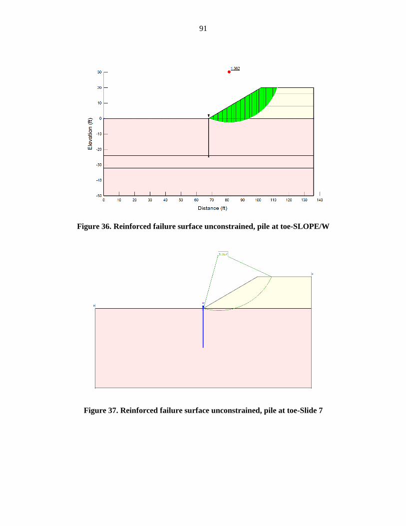
91
Figure 36. Reinforced failure surface unconstrained, pile at toe-SLOPE/W
Figure 37. Reinforced failure surface unconstrained, pile at toe-Slide 7

92
Figure 38. Reinforced Failure Surface Unconstrained, Pile in the Middle SLOPE/W
Figure 39. Reinforced Failure Surface Unconstrained, Pile in the Middle Reinforced Slide 7

93
The final location of the critical surface from the unconstrained reinforced condition was
15.8ft below the top of the pile (approximately 5.8ft from the ground surface). The results show
the difference between the assumed sliding depth (9ft) and the value achieved after placing the
piles. The magnitude of the stabilizing forces is significantly influence by the depth of the sliding
surface.
Table 18. Summary of results reinforced analises to achived F.S. = 1.4
Condition Shear force (lbs)
Shear force
Unfactored
(Method A)
(lbs)
Pile location
Constrained
(SLOPE/W) 6,720 4800
Toe Constrained
(Slide 7) 6,720 4800
Unconstrained
(SLOPE/W) F.S. not achieved Toe
Unconstrained
(Slide 7)
Unconstrained
(SLOPE/W) 8,540 6100
Middle Unconstrained
(Slide 7) 8,775 6268
In the next section the optimal pile location and depth will be determined based on the
required shear to stabilize the slope to the target factor of safety.
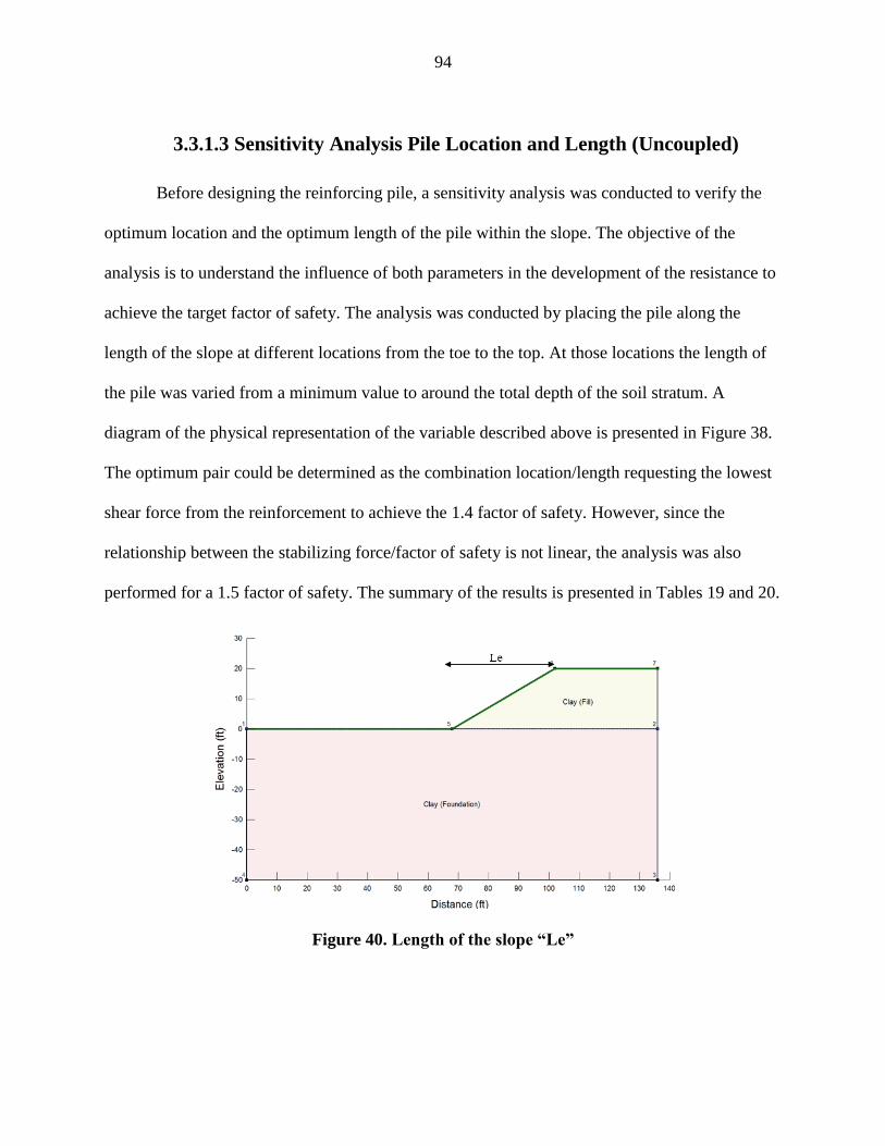
94
3.3.1.3 Sensitivity Analysis Pile Location and Length (Uncoupled)
Before designing the reinforcing pile, a sensitivity analysis was conducted to verify the
optimum location and the optimum length of the pile within the slope. The objective of the
analysis is to understand the influence of both parameters in the development of the resistance to
achieve the target factor of safety. The analysis was conducted by placing the pile along the
length of the slope at different locations from the toe to the top. At those locations the length of
the pile was varied from a minimum value to around the total depth of the soil stratum. A
diagram of the physical representation of the variable described above is presented in Figure 38.
The optimum pair could be determined as the combination location/length requesting the lowest
shear force from the reinforcement to achieve the 1.4 factor of safety. However, since the
relationship between the stabilizing force/factor of safety is not linear, the analysis was also
performed for a 1.5 factor of safety. The summary of the results is presented in Tables 19 and 20.
Figure 40. Length of the slope “Le”

95
Table 19. Summary Required Shear (lbs) for achiving F.S.=1.4
Location
Pile length (ft)
16 20 24 26 28 30 35 40
Toe Pile in the toe does not reach F.S.=1.4
Le/4 NR* 8,700 8,700 8,700 8,700 8,700 8,700 8,700
Le/2 NR NR NR 8,750 8,750 8,750 8,750 8,750
(3/4)Le NR NR NR NR 10,500 10,500 10,500 10,500
Top NR NR NR NR 11,000 11,000 11,000 11,000
*NR means F.S. not reached
*Ultimate
Table 20. Summary Required Shear for achiving F.S.=1.5
Location
Pile length (ft)
16 20 24 26 28 30 35 40
Toe Pile in the toe does not reach F.S.=1.5
Le/4 NR* NR NR 13,600 13,600 13,600 13,600 13,600
Le/2 NR NR NR NR NR 13,500 13,500 13,500
(3/4)Le NR NR NR NR NR NR 14,400 14,400
Top Pile in the top does not reach F.S.=1.5
*NR means F.S. not reached
*Allowable
From the results presented in Table 19 and 20, locating the pile at the toe does not
represent a favorable condition since the target factors of safety could not be reached even at
higher shear values. In the same way, the results also show that for relative higher improvement
in the F.S., locating the pile at the top also represents an unfavorable condition. The highest F.S.
at the top for high shear values was 1.43. Pile lengths with embedment depth below 20ft (from
the horizontal ground to the pile tip, ratio sliding depth/pile length below 0.3 for F.S.=1.4 and
0.45 for F.S.=1.5) also fail in achieving the target F.S.s. The results indicate that every pile

96
length will reach a maximum factor of safety no matter the shear capacity. Thus, to increase the
factor of safety in that situation the total length should be also increased.
Furthermore, piles located around Le/4 and Le/2 with embedment length equal or greater
that 20ft yields the most favorable results for both cases. However, the minimum required shear
force from the reinforcement was found when the pile is located at Le/4 for pile length equal or
larger than 20ft (for F.S.=1.4). The same configuration did not meet the requirements for
F.S.=1.5 indicating again that an appropriate embedment length must be assured to increase the
factor of safety. When piles are located from the toe to the top, the total length must be increased
so that the minimum embedment depth is assured. Thus, the optimum combination for both
factors of safety is considerably different. On one hand, the optimum position will be at a
distance around the quarter of the slope, with very small difference with the values from the
middle of the slope, when the shear wants to be minimized at smaller pile lengths. On the other
hand, the optimal location of the pile would be in the middle of the slope when higher factors of
safety are targeted.
To graphically understand the relationship between F.S. and shear loads to select the
condition that maximize factor of safety and minimize the shear loads, the optimum pile lengths
from the results in Tables 19 and 20 are used to determine several F.S./loads and have been
plotted presented in Figure 41. Moreover, when the optimum length of a pile for x condition has
been reached, increasing the embedment length will no produced any favorable effect on the
required shear to achieve a desirable factor of safety (if the pile length is increased beyond x
value but the shear is kept constant).
From combining Tables 19 and 20 with Figure 41 the following trends can be seen, for
small improvement on the factor of safety, all pile locations will yield favorable results. For
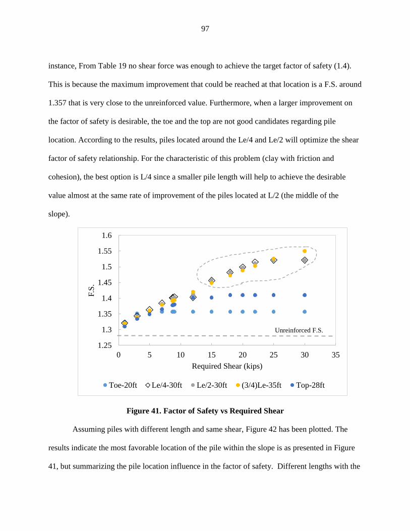
97
instance, From Table 19 no shear force was enough to achieve the target factor of safety (1.4).
This is because the maximum improvement that could be reached at that location is a F.S. around
1.357 that is very close to the unreinforced value. Furthermore, when a larger improvement on
the factor of safety is desirable, the toe and the top are not good candidates regarding pile
location. According to the results, piles located around the Le/4 and Le/2 will optimize the shear
factor of safety relationship. For the characteristic of this problem (clay with friction and
cohesion), the best option is L/4 since a smaller pile length will help to achieve the desirable
value almost at the same rate of improvement of the piles located at L/2 (the middle of the
slope).
Figure 41. Factor of Safety vs Required Shear
Assuming piles with different length and same shear, Figure 42 has been plotted. The
results indicate the most favorable location of the pile within the slope is as presented in Figure
41, but summarizing the pile location influence in the factor of safety. Different lengths with the
1.25
1.3
1.35
1.4
1.45
1.5
1.55
1.6
0 5 10 15 20 25 30 35
F.S
.
Required Shear (kips)
Toe-20ft Le/4-30ft Le/2-30ft (3/4)Le-35ft Top-28ft
Unreinforced F.S.
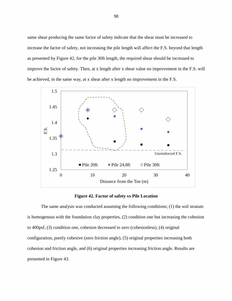
98
same shear producing the same factor of safety indicate that the shear must be increased to
increase the factor of safety, not increasing the pile length will affect the F.S. beyond that length
as presented by Figure 42, for the pile 30ft length, the required shear should be increased to
improve the factor of safety. Then, at x length after x shear value no improvement in the F.S. will
be achieved, in the same way, at x shear after x length no improvement in the F.S.
Figure 42. Factor of safety vs Pile Location
The same analysis was conducted assuming the following conditions; (1) the soil stratum
is homogenous with the foundation clay properties, (2) condition one but increasing the cohesion
to 400psf, (3) condition one, cohesion decreased to zero (cohesionless), (4) original
configuration, purely cohesive (zero friction angle), (5) original properties increasing both
cohesion and friction angle, and (6) original properties increasing friction angle. Results are
presented in Figure 43.
1.25
1.3
1.35
1.4
1.45
1.5
0 10 20 30 40
F.S
.
Distance from the Toe (m)
Pile 20ft Pile 24.8ft Pile 30ft
Unreinforced F.S.
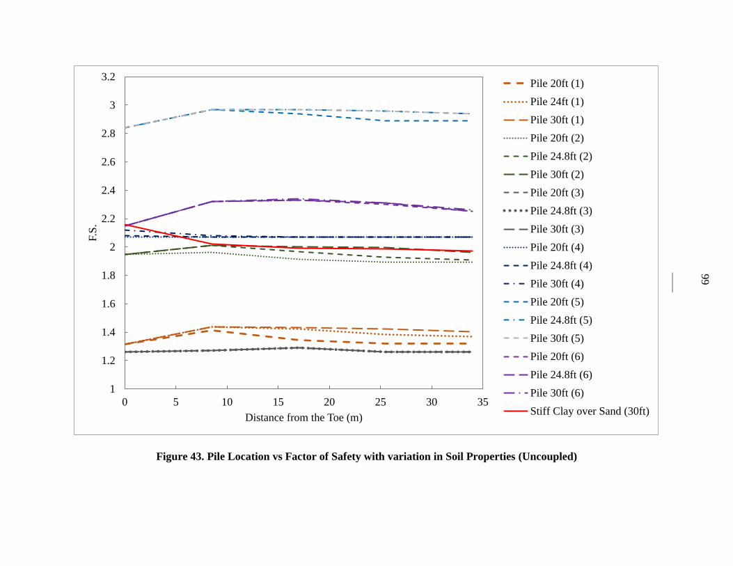
99
Figure 43. Pile Location vs Factor of Safety with variation in Soil Properties (Uncoupled)
1
1.2
1.4
1.6
1.8
2
2.2
2.4
2.6
2.8
3
3.2
0 5 10 15 20 25 30 35
F.S
.
Distance from the Toe (m)
Pile 20ft (1)
Pile 24ft (1)
Pile 30ft (1)
Pile 20ft (2)
Pile 24.8ft (2)
Pile 30ft (2)
Pile 20ft (3)
Pile 24.8ft (3)
Pile 30ft (3)
Pile 20ft (4)
Pile 24.8ft (4)
Pile 30ft (4)
Pile 20ft (5)
Pile 24.8ft (5)
Pile 30ft (5)
Pile 20ft (6)
Pile 24.8ft (6)
Pile 30ft (6)
Stiff Clay over Sand (30ft)

100
The results strongly indicate that the optimum location of a pile within a slope depends
on the properties of the materials. For soils predominantly cohesive, the difference in the factors
of safety for piles at different locations along the slope length is considered minimal. For purely
cohesive soils the same trend is followed with a slightly higher factor of safety for the pile
located at the toe (4 and clay over sand cases). For soils predominantly cohesionless, the
optimum location changes to around the quarter and the middle going to the upper portion of the
slope as the friction increases. In addition, the differences in the factors of safety for the various
locations become significant as the friction angle increases and smaller as the cohesion increases.
Thus, for combined materials (with friction and cohesion) the differences in the factors of safety
will be controlled by the dominant parameter. This could be related to the strength of the
materials since frictional materials are generally stronger than cohesive materials.
As mention in section 2.4.2, for a soil with a large cohesion and a small friction angle,
the most critical failure surface will be a deep circle, while shallow circle will be the critical slide
surface for a soil with a small cohesion and a large friction angle material (Huang 2014,
NAVFAC (1986). Hence, as cohesion increases the critical circle moves deeper. In contrast, as
friction angle increases, the critical circle moves upward making certain places of the slope (like
the toe) less suitable for the pile location.
The results show that if the material within the slope is sandy soil the optimum pile
location is clearly the middle (a shallow critical surface is developed). In contrast, for the
opposite condition the optimum location will be the toe (slightly higher factor of safety than the
other locations). For a slope with sand and cohesive foundation, the critical circle depends on
the consistency of the cohesive material. Sand over soft clay will develop a deep critical circle
and sand over stiff clay will most likely develop a shallow sliding surface. Thus, for the first case

101
the optimum location will be around the toe and for the second one from the middle to the top.
This is consistent with the findings for a slope with stiff clay over soft clay and vice versa. The
deepest critical circle generated through the weakest soil layer will generally require the piles to
be located around the toe.
For the uncoupled analysis, it can be said that because most soils in nature are
combined, the weakest material will govern the failure surface position. Small values of cohesion
in a material may suggest that the dominant behavior will be frictional and that the pile optimum
location will range around the quarter and the middle moving upslope with higher values of
friction angle. Cases 1, 2, and 5 show that increments of 100psf in cohesion reduces the gap
between factors of safety for piles a different distances from the toe, suggesting that for cohesive
soils a pile could be located in any place, with the toe a slightly better location. This allows for
constructability freedom where the optimum pile location could be selected in terms of the
convenient location regarding access, equipment, previous experience of contractors, among
others. The presence of stiff cohesive materials changes the optimum location of a pile regarding
the location of the stronger material (stiff material in the top, the pile should be placed around the
toe, stiff clay in the foundation, pile location around the middle and upper portion).
A summary regarding the key findings from the sensitivity analysis is presented in Table
21. The trends suggest that overall the optimum location of a pile depends on the elevation of the
sliding depth which at the same time depends upon the consistency of the materials within the
slope. For the case of cohesive materials, the improvement on the F.S. among locations is
considerably small and engineering judgement must be used to determine the most convenient
location in terms of constructability.
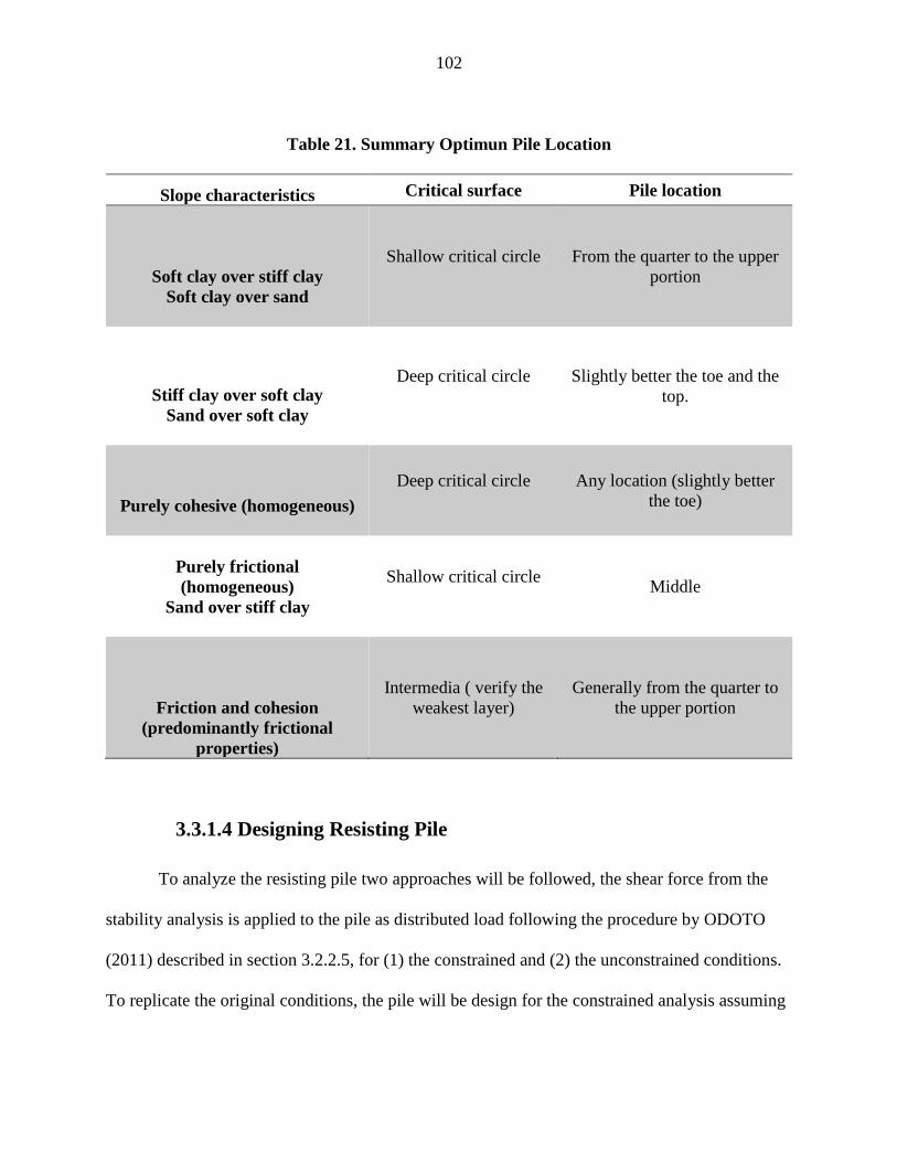
102
Table 21. Summary Optimun Pile Location
Slope characteristics Critical surface Pile location
Soft clay over stiff clay
Soft clay over sand
Shallow critical circle
From the quarter to the upper
portion
Stiff clay over soft clay
Sand over soft clay
Deep critical circle
Slightly better the toe and the
top.
Purely cohesive (homogeneous)
Deep critical circle
Any location (slightly better
the toe)
Purely frictional
(homogeneous)
Sand over stiff clay
Shallow critical circle
Middle
Friction and cohesion
(predominantly frictional
properties)
Intermedia ( verify the
weakest layer)
Generally from the quarter to
the upper portion
3.3.1.4 Designing Resisting Pile
To analyze the resisting pile two approaches will be followed, the shear force from the
stability analysis is applied to the pile as distributed load following the procedure by ODOTO
(2011) described in section 3.2.2.5, for (1) the constrained and (2) the unconstrained conditions.
To replicate the original conditions, the pile will be design for the constrained analysis assuming
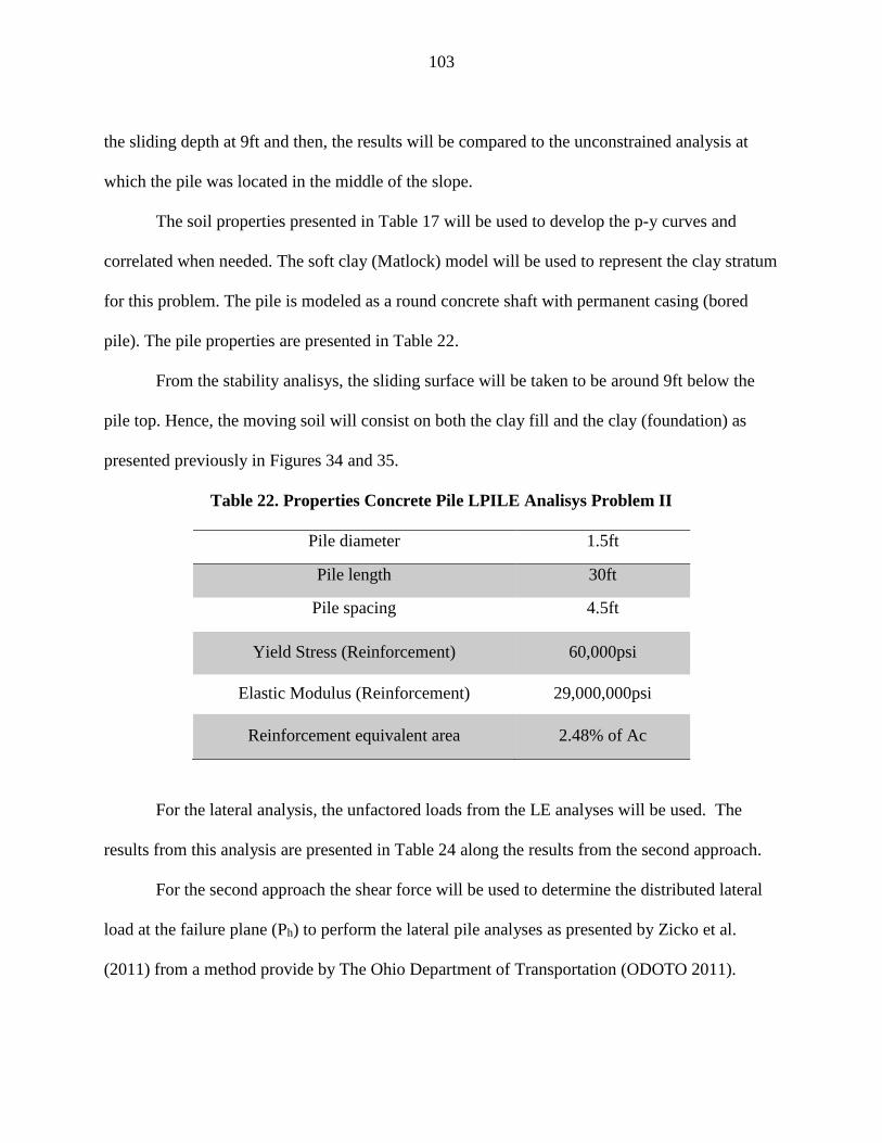
103
the sliding depth at 9ft and then, the results will be compared to the unconstrained analysis at
which the pile was located in the middle of the slope.
The soil properties presented in Table 17 will be used to develop the p-y curves and
correlated when needed. The soft clay (Matlock) model will be used to represent the clay stratum
for this problem. The pile is modeled as a round concrete shaft with permanent casing (bored
pile). The pile properties are presented in Table 22.
From the stability analisys, the sliding surface will be taken to be around 9ft below the
pile top. Hence, the moving soil will consist on both the clay fill and the clay (foundation) as
presented previously in Figures 34 and 35.
Table 22. Properties Concrete Pile LPILE Analisys Problem II
Pile diameter 1.5ft
Pile length 30ft
Pile spacing 4.5ft
Yield Stress (Reinforcement) 60,000psi
Elastic Modulus (Reinforcement) 29,000,000psi
Reinforcement equivalent area 2.48% of Ac
For the lateral analysis, the unfactored loads from the LE analyses will be used. The
results from this analysis are presented in Table 24 along the results from the second approach.
For the second approach the shear force will be used to determine the distributed lateral
load at the failure plane (Ph) to perform the lateral pile analyses as presented by Zicko et al.
(2011) from a method provide by The Ohio Department of Transportation (ODOTO 2011).
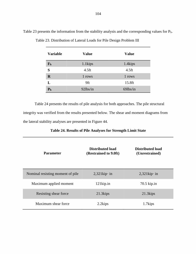
104
Table 23 presents the information from the stability analysis and the corresponding values for Ph.
Table 23. Distribution of Lateral Loads for Pile Design Problem III
Variable Value Value
Fh 1.1kips 1.4kips
S 4.5ft 4.5ft
R 1 rows 1 rows
L 9ft 15.8ft
Ph 92lbs/in 69lbs/in
Table 24 presents the results of pile analysis for both approaches. The pile structural
integrity was verified from the results presented below. The shear and moment diagrams from
the lateral stability analyses are presented in Figure 44.
Table 24. Results of Pile Analyses for Strength Limit State
Parameter
Distributed load
(Restrained to 9.0ft)
Distributed load
(Unrestrained)
Nominal resisting moment of pile 2,321kip· in 2,321kip· in
Maximum applied moment 121kip.in 70.5 kip.in
Resisting shear force 21.3kips 21.3kips
Maximum shear force 2.2kips 1.7kips

105
Pile at the Toe-failure surface 9ft
Pile at the middle-Failure surface 15.8ft
Figure 44. Bending Moment and Shear from Lateral Analysis
106
3.3.2 Coupled analysis
For this analysis, the unreinforced analysis will also be performed to verify if the target
factor of safety is reached (as presented in section 3.3.1.1). The reinforced analysis will then be
conducted after placing the reinforcing pile in both positions the toe and the middle of the slope
as in the uncouple analysis.
3.3.2.1 Unreinforced Analysis
The unreinforced factor of safety for this condition has been determined from the 2-
dimensional elasto-plastic finite element analysis by the shear strength reduction method using
Phase2. Additional results are also presented from the analysis in the finite difference program
FLAC.
Figure 45 presents the factor of safety and the location of the critical failure surface from
the LE analysis in superposition with the critical circle from the LE analysis performed in Slide
7.0 presented in section 3.3.1.1. The results show high compatibility between the location of the
critical circle and the factors of safety. For the LE analysis in Slide 7.0, F.S.=1.311 while from
Phase2 the SSR was 1.29.
Furthermore, the results from the FD analysis performed in FLAC are presented in Figure
48. The deformed mesh indicates that the location of the critical circle is also consistent with the
results from Phase2.

107
Figure 45. Superposition Unreinforced Analysis Phase2 and Slide 7.0
Figure 46. Unreinforced Analysis FLAC (F.S.=1.33)

108
3.3.2.2 Reinforced Analysis
In phase2, the piles were modeled using structural interfaces with a joint on either side of
the reinforcement (liner)allowing slip to occur between the reinforcement and the soil
(Rocscience Inc. 2017). Pile properties for both FE and FD analysis are presented in Table 25.
The soil properties are the same from the LE analysis.
Table 25. Properties SSR Analysis Phase2 and FLAC
Parameter Magnitude
Pile length 30ft
Pile spacing 4.5ft
Pile diameter 1.5ft
Young’s modulus 3605(ksi)
Poisson’s ratio 0.15
Yield Strength (f’c) 4000psi
Tensile strength 350psi
The results are presented in Figures 47 and 48 for the pile placed at the toe. To verify
which one would be the optimum pile location a sensitivity analysis will be presented in the next
section. However, Figures 49 and 50 present the results for the pile placed in the middle. A
considerable difference is found between the results from FLAC and Phase2, additional analysis
should be done to determine if the boundary conditions when the pile is located at the middle of
the slope for both analysis have been considered the same (either free in both sides of the slope
or restricted below or above the pile).

109
Figure 47. Reinforced Analysis Phase2 Pile in the Toe
Figure 48. Reinforced Analysis FLAC Pile in the Toe (F.S.=1.35)

110
Figure 49. Reinforced Analysis Phase2 Pile in the Middle
Figure 50. Reinforced Analysis FLAC Pile in the Toe (F.S.=1.99)

111
3.3.2.3 Sensitivity Analysis (Coupled)
As in the uncoupled analysis, for the coupled one, the pile will also be located at different
locations within the slope to verify the optimum location from FE analysis. Conditions
considered include: (1) the soil stratum is homogenous with the foundation clay properties, (2)
condition one but increasing the cohesion to 400psf, (3) condition one, cohesion decreased to
zero, (4) original configuration and purely cohesive and (5) original properties increasing both
cohesion and friction angle, and (6) original properties increasing friction angle, will also be
analyzed. The results are presented in Figure 51 for the original problem and Figure 52 for the
additional conditions.
Figure 51. Pile Location Versus Factor of safety
1.2
1.25
1.3
1.35
1.4
1.45
1.5
0 10 20 30 40
F.S
.
Distance from the Toe (m)
Pile 20ft
Pile 24.8ft
Pile 30ft
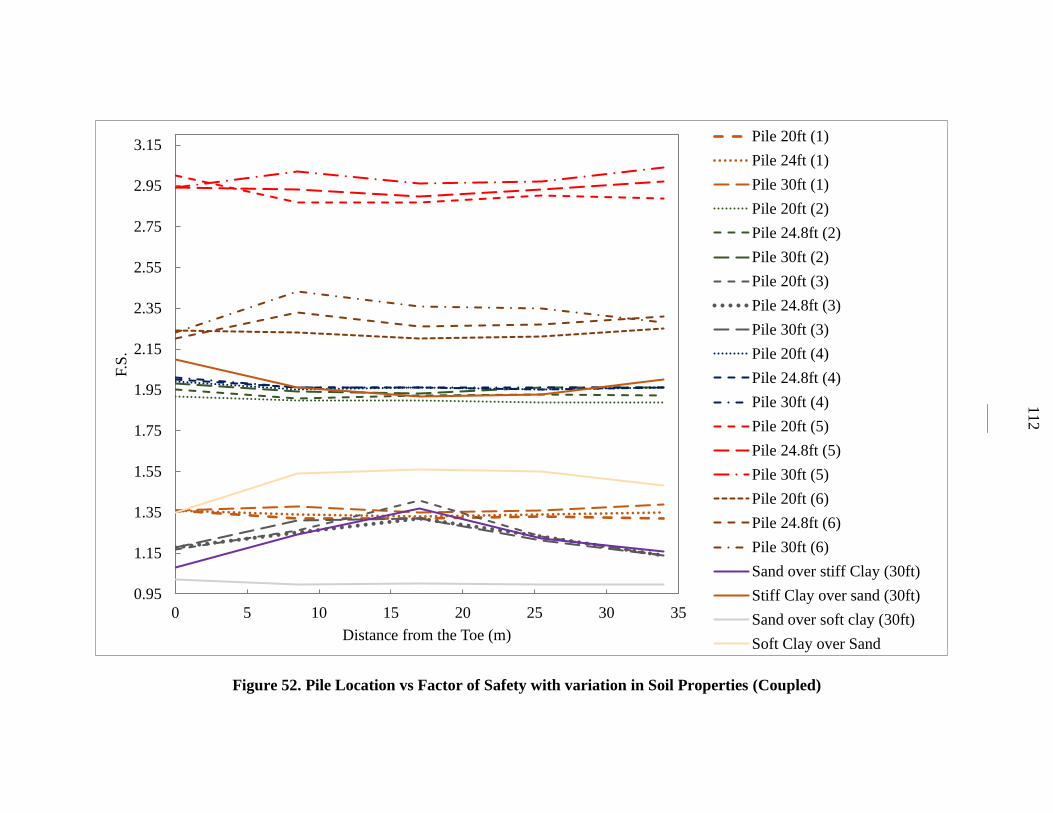
112
Figure 52. Pile Location vs Factor of Safety with variation in Soil Properties (Coupled)
0.95
1.15
1.35
1.55
1.75
1.95
2.15
2.35
2.55
2.75
2.95
3.15
0 5 10 15 20 25 30 35
F.S
.
Distance from the Toe (m)
Pile 20ft (1)
Pile 24ft (1)
Pile 30ft (1)
Pile 20ft (2)
Pile 24.8ft (2)
Pile 30ft (2)
Pile 20ft (3)
Pile 24.8ft (3)
Pile 30ft (3)
Pile 20ft (4)
Pile 24.8ft (4)
Pile 30ft (4)
Pile 20ft (5)
Pile 24.8ft (5)
Pile 30ft (5)
Pile 20ft (6)
Pile 24.8ft (6)
Pile 30ft (6)
Sand over stiff Clay (30ft)
Stiff Clay over sand (30ft)
Sand over soft clay (30ft)
Soft Clay over Sand

113
The results from Figure 51 indicate that the factor of safety variation with pile location is
considerably small being the around the toe and the top the slightly better locations and the
quarter of the slope for larger piles. The findings are partially consistent with the results from
section 3.3.1.3, indicating that from FE analysis the material is predominately cohesive. From the
additional analyses, the same trends of the uncoupled analysis are seen. For purely frictional
slopes the optimum location will be around the middle, for purely cohesive slopes the pile could
be located at any place being the toe the slightly better condition. For materials with friction and
cohesion, the optimum location will be from the quarter of the slope to the upper portion if
frictions govern and any location of the slope if cohesion increases.
The results from both analyses, coupled and uncoupled, relate with the previously
published conclusions from several authors presented in Table 5. The authors specified different
pile locations regarding the case they were presenting. Comparing the individual results to the
present study, the relationship between pile location and soil type become evident. For the cases
where the soil correspond to combined with friction and cohesion (with dominant frictional
behavior) the optimum location was reported mostly from the middle to the upper portion, and
for cases were the soils where predominately cohesive several authors consistently recommended
the pile to be located at either the toe or the top. Most authors indicate the middle of the slope as
the optimum location because of the characteristics of the materials within the slope they were
studying (generally intermediate materials with relatively lower cohesion and average friction
angle).
Additional research must be conducted to verify how the factor of safety responses to the
simultaneous increment of cohesion and friction can be independently characterized. In addition,

114
the results from the present study should be validated from parametric studies conducted in
others finite element or finite difference programs.
3.3.3 Summary Results Coupled and Uncoupled Analyses Problem II
An overall summary is presented in Table 26. The ultimate factor of safety refers to the
value after performing stability analysis with the shear values from LPILE (for uncoupled
analysis). Thus, for the coupled analysis, the value will be original reinforced factor of safety.
The results are normalized by 1ft width of soil.
Table 26. General Summary Problem II
Condition Unreinforced
F.S.
Reinforced
F.S.
**Required
Shear
(kips)
*Shear
at the
Sliding
depth
(kips)
Max.
Moment
(kips.in)
Ultimate
F.S.
SLOPE/W-
9ft 1.354 1.4 1.1
0.4 89 1.37
Slide 7-9ft 1.357 1.1
SLOPE/W-
Middle 1.316 1.4 1.4
0.4 70.5 1.34 Slide 7-
Middle 1.311 1.4
Phase2
(Toe) 1.29
1.39 - 1.2 146.4 1.39
Phase2
(Middle) 1.37 - 1.3 80.1 1.37
FLAC
(Toe) 1.33
1.35 - 0.1 31 1.35
FLAC
(Middle) 1.99*** - 3.6 248 1.99
**The values presented come from LE programs
***The values presented come from either LPILE for uncoupled analysis or FE, FD programs
*** Should be verified

115
For the unreinforced analyses, all methods of analysis achieved around the same factor of
safety. Thus, LE, FE, or FD programs are comparatively recommended regarding accuracy and
reliability. The influence of assuming a fixed critical surface can be seen. However, the
difference between the constrained and unconstrained values is practically negligible with the
F.S. from the assumed depth slightly more conservative.
For the reinforced analyses, the shear resistance developed by the pile and the factor of
safety can be compared. On one hand, the shear resistances from LPILE (for uncoupled
condition) are considerably different from the values from the Phase2 and FLAC. However, the
ultimate factors of safety from coupled and uncoupled analysis are similar. As in section 3.2.3,
the ultimate factor of safety of an uncoupled analysis was found lower than the target factor since
the resistance of the pile was not developed a hundred percent. The results from FLAC when the
pile is placed in the middle of the slope must be investigated in more detail because of the larger
difference between shear, moment and factors of safety with the other conditions.
Overall, the ultimate factors of safety are similar. Thus, performing a coupled or
uncoupled pile reinforced slope analysis will yield similar results.
For the optimum pile location, by comparing the results from Sections 3.3.2.3 and
3.3.3.3, the coupled and uncoupled conditions produce similar results. Piles must be located with
consideration of the critical sliding depth. For soils in which friction is predominant, the
optimum location will be around the middle and the upper portion of the slope if adequate
embedment depth is assured. To assure that the embedment is adequate a sensitivity analysis
should be conducted. Piles located from the middle to upper portion will require larger lengths to
maintain the embedment length.
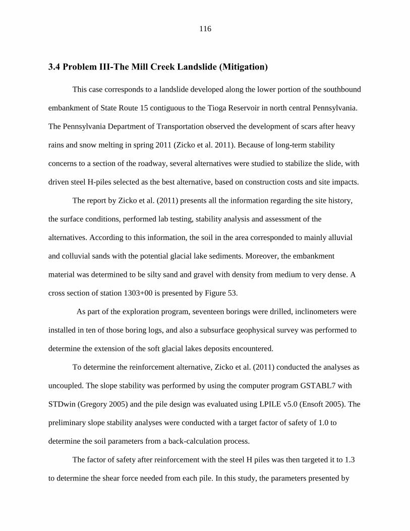
116
3.4 Problem III-The Mill Creek Landslide (Mitigation)
This case corresponds to a landslide developed along the lower portion of the southbound
embankment of State Route 15 contiguous to the Tioga Reservoir in north central Pennsylvania.
The Pennsylvania Department of Transportation observed the development of scars after heavy
rains and snow melting in spring 2011 (Zicko et al. 2011). Because of long-term stability
concerns to a section of the roadway, several alternatives were studied to stabilize the slide, with
driven steel H-piles selected as the best alternative, based on construction costs and site impacts.
The report by Zicko et al. (2011) presents all the information regarding the site history,
the surface conditions, performed lab testing, stability analysis and assessment of the
alternatives. According to this information, the soil in the area corresponded to mainly alluvial
and colluvial sands with the potential glacial lake sediments. Moreover, the embankment
material was determined to be silty sand and gravel with density from medium to very dense. A
cross section of station 1303+00 is presented by Figure 53.
As part of the exploration program, seventeen borings were drilled, inclinometers were
installed in ten of those boring logs, and also a subsurface geophysical survey was performed to
determine the extension of the soft glacial lakes deposits encountered.
To determine the reinforcement alternative, Zicko et al. (2011) conducted the analyses as
uncoupled. The slope stability was performed by using the computer program GSTABL7 with
STDwin (Gregory 2005) and the pile design was evaluated using LPILE v5.0 (Ensoft 2005). The
preliminary slope stability analyses were conducted with a target factor of safety of 1.0 to
determine the soil parameters from a back-calculation process.
The factor of safety after reinforcement with the steel H piles was then targeted it to 1.3
to determine the shear force needed from each pile. In this study, the parameters presented by

117
Zicko et al. (2011) will be used to performed a coupled and uncoupled analysis. A summary of
the soil properties is presented in Table 27.
Figure 53. Subsurface Profile along the Critical cross-section at Station 1303+00 after
Zicko et al. (2011)
From the laboratory testing, the glacial lake deposit was found to have residual and peak
strengths that were fixed to determine the additional soil properties from the back analysis.

118
Table 27. Soil Properties Mill Creek Landslide after Zicko et al. (2011)
3.4.1 Uncoupled Analysis
For the uncoupled analysis, slope stability and pile analysis are presented. First, the factor
of safety of the unreinforced slope is verified to be 1.0 since the soil parameters come from back
analysis calculations. Two different analyses will be performed by (1) analyzing the
unconstrained slope to verify the potential location of the failure surface, and (2) analyzing the
failure surface constrained to the location of the in situ scars (as conducted in the report). The
factor of safety will then be targeted to 1.3 following the procedure by Zicko et al. (2011) to
determine the necessary shear force from the reinforcing pile. Furthermore, the pile analysis will
be conducted.
3.4.1.1 Unreinforced Analysis
As stated before, the first unreinforced analysis will be done to verify the potential
location of the failure surface under the given soil conditions, if no in situ information of the scar
Soil type
Total Unit
Weight
(pcf)
c'
(kPa) Φ' ()
Embankment Fill 120 0 32
Colluvial 120 0 30
Peak ML 120 0 25
SM cobbl 125 0 36
Residual ML 120 0 16
Glacial 130 0 38
Rockfill 130 0 45
Colluvial 2 120 0 34
Residual Colluvial 120 0 28
Residual SM cobbl 125 0 30
Residual Rockfill 130 0 38
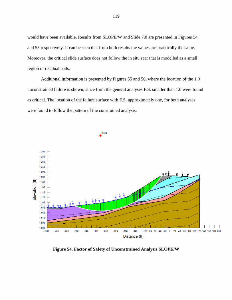
119
would have been available. Results from SLOPE/W and Slide 7.0 are presented in Figures 54
and 55 respectively. It can be seen that from both results the values are practically the same.
Moreover, the critical slide surface does not follow the in situ scar that is modelled as a small
region of residual soils.
Additional information is presented by Figures 55 and 56, where the location of the 1.0
unconstrained failure is shown, since from the general analyses F.S. smaller than 1.0 were found
as critical. The location of the failure surface with F.S. approximately one, for both analyses
were found to follow the pattern of the constrained analysis.
Figure 54. Factor of Safety of Unconstrained Analysis SLOPE/W
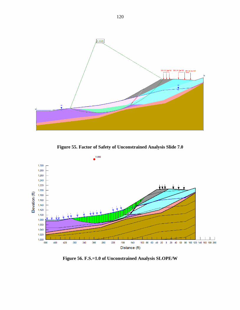
120
Figure 55. Factor of Safety of Unconstrained Analysis Slide 7.0
Figure 56. F.S.=1.0 of Unconstrained Analysis SLOPE/W

121
Figure 57. F.S.=1.0 of Unconstrained Analysis Slide 7.0
On the other hand, the results from the constrained analysis are presented in Figures 58
and 59. The target value F.S. equal to 1.0 is achieved by following the scar developed at the
time of failure.
Figure 58. Factor of Safety of Unconstrained Analysis SLOPE/W

122
Figure 59. Factor of Safety of Constrained Analysis Slide 7.0
3.4.1.2 Reinforced Analysis
After the unreinforced analysis is conducted, a reinforced analysis with the calibrated to
1.0 factor of safety failure surface is conducted. The target factor of safety is 1.30. The section
determined as the most viable option (H-Piles 12x53) was evaluated and the shear forces from
the current analyses are compared with the original values. Because the original program
(GSTABL7 by Gregory (2005)) includes the stabilizing force in the numerator to calculate the
factor of safety, the method that will be used to determine the reinforcement load will be
“Method B”. The target value was achieved for 65 kips for both SLOPE/W and Slide 7.0. The
factor of safety was also evaluated for the shear presented by Zicko et al. (2011) 75 kips. The
resulting value was 1.32 and because both values are very similar, the design of the pile will be
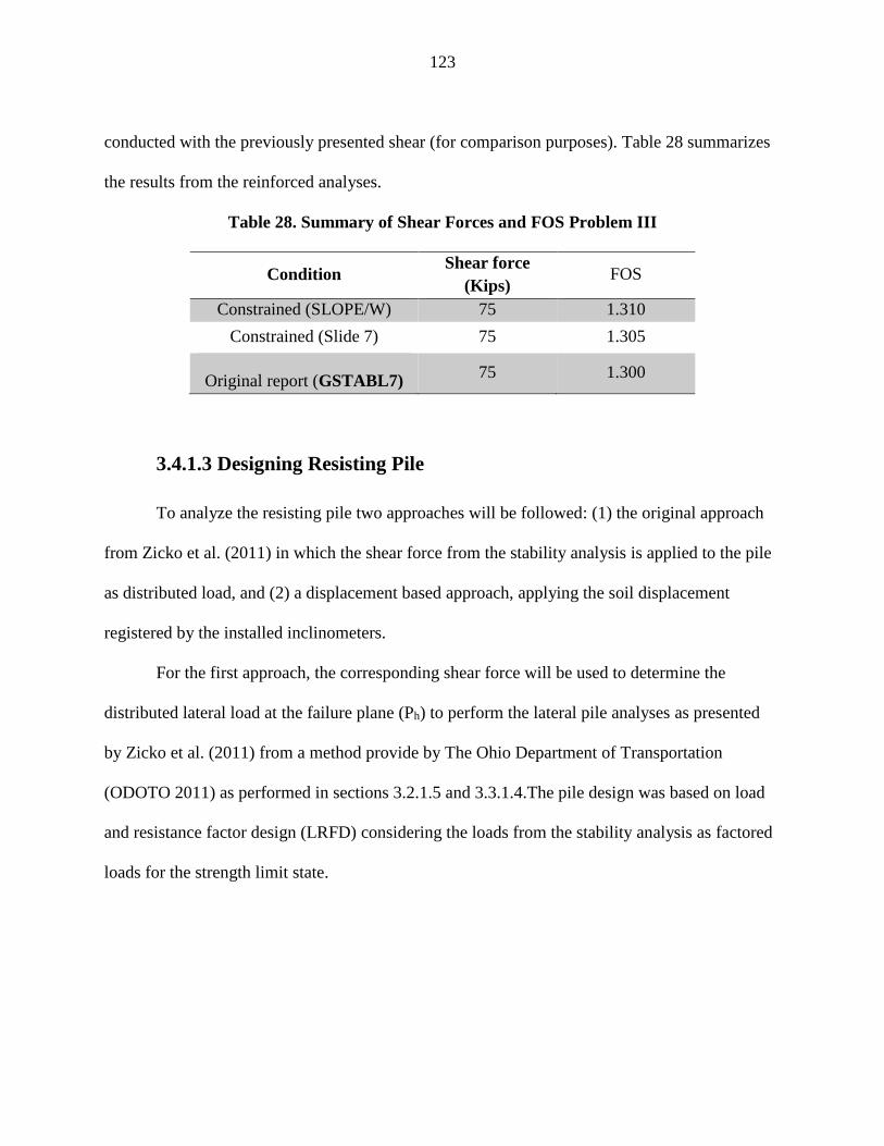
123
conducted with the previously presented shear (for comparison purposes). Table 28 summarizes
the results from the reinforced analyses.
Table 28. Summary of Shear Forces and FOS Problem III
Condition Shear force
(Kips) FOS
Constrained (SLOPE/W) 75 1.310
Constrained (Slide 7) 75 1.305
Original report (GSTABL7) 75 1.300
3.4.1.3 Designing Resisting Pile
To analyze the resisting pile two approaches will be followed: (1) the original approach
from Zicko et al. (2011) in which the shear force from the stability analysis is applied to the pile
as distributed load, and (2) a displacement based approach, applying the soil displacement
registered by the installed inclinometers.
For the first approach, the corresponding shear force will be used to determine the
distributed lateral load at the failure plane (Ph) to perform the lateral pile analyses as presented
by Zicko et al. (2011) from a method provide by The Ohio Department of Transportation
(ODOTO 2011) as performed in sections 3.2.1.5 and 3.3.1.4.The pile design was based on load
and resistance factor design (LRFD) considering the loads from the stability analysis as factored
loads for the strength limit state.
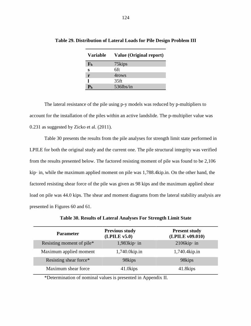
124
Table 29. Distribution of Lateral Loads for Pile Design Problem III
Variable Value (Original report)
Fh 75kips
s 6ft
r 4rows
l 35ft
Ph 536lbs/in
The lateral resistance of the pile using p-y models was reduced by p-multipliers to
account for the installation of the piles within an active landslide. The p-multiplier value was
0.231 as suggested by Zicko et al. (2011).
Table 30 presents the results from the pile analyses for strength limit state performed in
LPILE for both the original study and the current one. The pile structural integrity was verified
from the results presented below. The factored resisting moment of pile was found to be 2,106
kip· in, while the maximum applied moment on pile was 1,788.4kip.in. On the other hand, the
factored resisting shear force of the pile was given as 98 kips and the maximum applied shear
load on pile was 44.0 kips. The shear and moment diagrams from the lateral stability analysis are
presented in Figures 60 and 61.
Table 30. Results of Lateral Analyses For Strength Limit State
Parameter Previous study
(LPILE v5.0)
Present study
(LPILE v09.010)
Resisting moment of pile* 1,983kip· in 2106kip· in
Maximum applied moment 1,740.0kip.in 1,740.4kip.in
Resisting shear force* 98kips 98kips
Maximum shear force 41.0kips 41.8kips
*Determination of nominal values is presented in Appendix II.
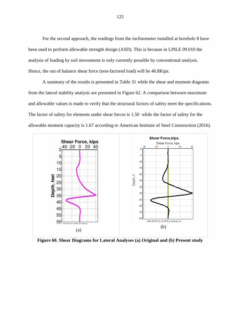
125
For the second approach, the readings from the inclinometer installed at borehole 8 have
been used to perform allowable strength design (ASD). This is because in LPILE 09.010 the
analysis of loading by soil movements is only currently possible by conventional analysis.
Hence, the out of balance shear force (non-factored load) will be 46.8Kips.
A summary of the results is presented in Table 31 while the shear and moment diagrams
from the lateral stability analysis are presented in Figure 62. A comparison between maximum
and allowable values is made to verify that the structural factors of safety meet the specifications.
The factor of safety for elements under shear forces is 1.50 while the factor of safety for the
allowable moment capacity is 1.67 according to American Institute of Steel Construction (2016).
(a)
(b)
Figure 60. Shear Diagrams for Lateral Analyses (a) Original and (b) Present study
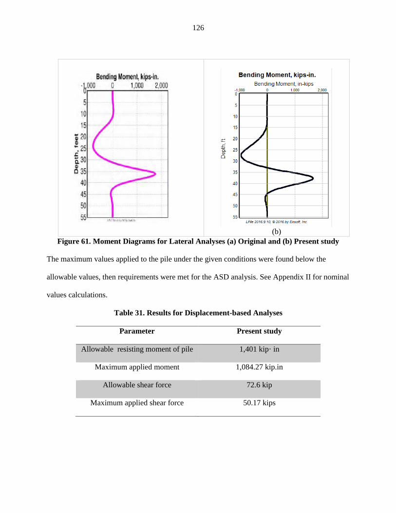
126
(b)
Figure 61. Moment Diagrams for Lateral Analyses (a) Original and (b) Present study
The maximum values applied to the pile under the given conditions were found below the
allowable values, then requirements were met for the ASD analysis. See Appendix II for nominal
values calculations.
Table 31. Results for Displacement-based Analyses
Parameter Present study
Allowable resisting moment of pile 1,401 kip· in
Maximum applied moment 1,084.27 kip.in
Allowable shear force 72.6 kip
Maximum applied shear force 50.17 kips
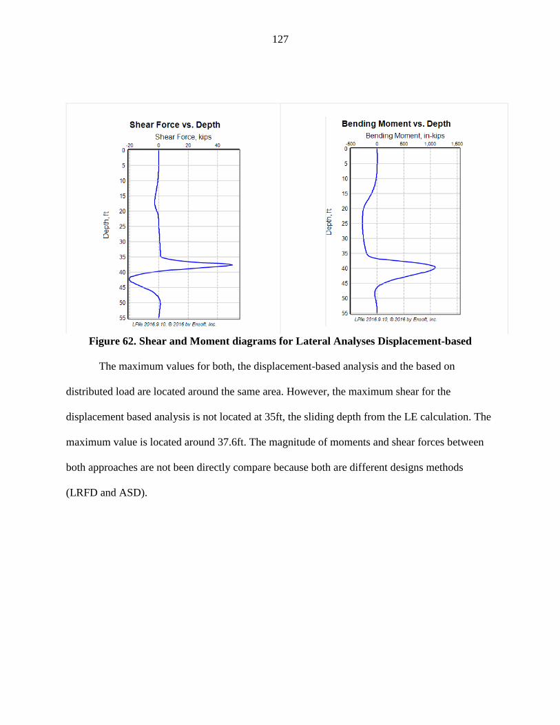
127
Figure 62. Shear and Moment diagrams for Lateral Analyses Displacement-based
The maximum values for both, the displacement-based analysis and the based on
distributed load are located around the same area. However, the maximum shear for the
displacement based analysis is not located at 35ft, the sliding depth from the LE calculation. The
maximum value is located around 37.6ft. The magnitude of moments and shear forces between
both approaches are not been directly compare because both are different designs methods
(LRFD and ASD).

128
3.4.2 Coupled Analysis
For this analysis, the unreinforced analysis will also be performed to verify the value of
the minimum factor of safety for the given soil conditions. Furthermore, the reinforced analysis
will then be conducted after placing the reinforcing pile as in the uncouple analysis.
3.4.2.1 Unreinforced Analysis
The unreinforced factor of safety for this condition is determined from the 2-dimensional
elasto-plastic finite element analysis by the shear strength reduction method using Phase2.
However, because the soil parameters used for this analysis come from the calibration of the
failure surface to 1.0, the minimum SSR was found smaller than 1.0. This indicates that the slope
is instable and no reduction of the shear strength could actually be done. Figure 63 presents the
critical SSR as well as the fitted critical slide surface from the LE analysis performed with Slide
7.0 in the uncoupled analysis. The critical region with the highest amount of soil movement is
represented by the orange-red zone and matches for both the Slide 7.0 and the Phase2 results.
If the critical slide for the factor of safety equal to 1.0 is superposed to Phase2’s results
for SSR equal to 1.0, agreement on the location of the critical zones in terms of soil movement is
also found as presented in Figure 64. The results indicate that the model should be calibrated to
1.0 in the FE program, hence, the soil properties from the uncoupled condition should vary until
the target F.S. is achieved.

129
Figure 63. Unreinforced Analysis Phase2
Figure 64. Unreinforced Analysis Phase2 for SSR equal to 1.0 and F.S. equal to 1.0 from
Slide 7.0

130
3.4.2.2 Reinforced Analysis
Because this model corresponds to an active failure, analysis in Phase2 found not
recommended. As presented in Figure 65, the value of the critical SSR from the unreinforced to
the reinforced analysis remains almost the same after the reinforcement is been placed. Results
from FLAC will be used as referenced of the couple analysis to compare with the uncoupled
section in future research.
Figure 65. Reinforced Analysis Phase2

131
3.4.3 Summary Results Coupled and Uncoupled Analyses Problem III
The overall results from this problem are presented in Table 32. The results indicate that
uncoupled analysis could be more advantageous when piles are located in an active failure zone.
This is because the assumptions of the location of the sliding surface are eliminated. The
displacement-based method when inclinometer data is available offers a reliable way of verifying
the results for pile structural analysis validating with the distributed load method.
Table 32. General Summary Problem III
Condition Unreinforced
F.S.
Reinforced
F.S.
Shear
Force
(kN/m)
Max. Shear
from
LPILE
(kN/m)
Max.
Moment
(kN.m)
Zicko et al.
(2011) 1.0 1.30 75 48 1,740.0
Slide 7 1.0 1.305
75
48.1(1)
50.1(2)
1,740.4(1)
1,084.3(2)
SLOPE/W 1.0 1.31
Phase2 0.7 - - - -
(1) Distributed load method
(2) Displacement-based
The accuracy of coupled analysis in active landslide should be investigated in detail with
different FE or FD programs.

132
CHAPTER 4. CONCLUSIONS AND RECOMMENDATIONS
4.1 Conclusions
In this study, comparative analyses has been conducted in order to investigate the relative
advantages, limitations, and accuracy of the current approaches for pile-reinforced slopes. The
analyses have been focused on determining the most advantageous option between coupled (pile
and slope in a sole analysis) and uncoupled (pile and slope in two different analysis) approach. In
addition, several sensitivity analyses were conducted for understanding the primary factors when
slopes reinforced by the means of pile elements are analyzed/design. From the results several
conclusions can be drawn:
(1) For unreinforced slopes, coupled and uncoupled analyses are equally recommended
regarding accuracy and reliability of the results.
(2) For reinforced slopes, the uncoupled analysis yields marginally more conservative
results when performed by the distributed load approach than by the displacement-
based method. However, the displacement-based method is better recommended
when in situ information is available. Overall, coupled and uncoupled analyses
produced similar factors of safety. In this study, the coupled approach is suggested as
the most beneficial. This is because several assumptions regarding location of sliding
depth, empirical representation of the soil (p-y curves for lateral analysis),
introduction of modifiers, and duplication of geotechnical and structural factors of
safety can be avoided. Moreover, when performing coupled analysis a unique
analysis is performed, iterations to determined optimum length and pile location are
easily done without distressing about assumptions of pile shear.

133
(3) In this study, the uncoupled approached is recommended when piles are analyzed as
mitigation alternative (active landslide), especially if the slope is instrumented and
displacement information is available.
(4) The coupled analysis required more parameters than the uncoupled. However, taking
into account the degree of effort to perform two separate analyses and to classify the
soil to develop p-y curves for the lateral analysis, the two approaches could be
considered equivalent or even more, if simple FE or FD models are studied, relative
little effort in terms of time consumption for model development is needed.
(5) The key factor to ensure accurate results from a coupled analysis is to represent the
studied condition as close as possible. This includes the soil conditions, the
constitutive model, and reliable values of the soil properties.
(6) If repeatability of the results is pursued, a coupled analysis can be performed and
either the shear resistance or soil displacement can be used into a limit equilibrium or
laterally loaded pile analysis program to verify the similarity of the results.
(7) Regarding the important factors when analyzing a pile-reinforced, because most
authors have previously presented consistent results regarding pile spacing, pile head
condition, pile length and number of rows, in this study the focus of the sensitivity
analysis was to determine the optimum pile location.
(8) The optimum location was found to depend on the critical surface location which at
the same time depends on the material within the slope. The weakest material
determine the location of the critical surface, if the sliding depth is considerably
shallow the piles must be located from the quarter to the upper portion of the slope
varying regarding the frictional characteristic of the materials (pure friction; middle,
134
friction and cohesion; generally from the quarter to the top, pure cohesion; generally
the toe but not very significant the factor of safety improvement with location). The
combination weak and soft material was found to produce similar effects on the
sliding depth for soft clay-stiff clay, soft clay-sand and sand-stiff clay.
(9) The recommended technique to determine optimum pile length is by performing
sensitivity analysis since the optimum length greatly depends on the slope
configuration. If an uncoupled analysis is conducted the optimum length should be
taken as the smaller depth at which the required shear is minimized and the factor of
safety is improved. In this study, to achieve a 1.4 factor of safety the optimum ratio
sliding depth/ pile length was found around 0.3 and around 0.45 to achieve a 1.5
factor of safety. From the coupled analysis, the optimum length could be seen from
the sensitivity analysis lying in a range where a sudden amount of shear resistance is
developed by the pile.
4.2 Recommendations for Future Research
The following recommendations are proposed to enhance the analytical work:
(1) To verify the equivalency of coupled and uncoupled factors of safety additional case
studies should be analyzed.
(2) To validate the results regarding optimum pile location several analyses must be
conducted using different computer programs, especially for combined materials
(with friction and cohesion) to separate the responses of the factor of safety to
variations in friction and cohesion.

135
(3) The efficiency of the coupled approach to analyze mitigation alternatives for an
active landslide must be studied to compare with the results of the uncoupled
approach.
(4) The group effect on piles, 3D effects, and soil arching by the coupled approach
should be studied since the investigations conducted in this analysis were mainly
focused on the analysis of piles in row and 2D analyses.
136
REFERENCES
American Institute of Steel Construction. (2016). “Specification for Structural Steel Buildings,
ANSI / AISC 360-16.” AMERICAN INSTITUTE OF STEEL CONSTRUCTION.
Ausilio, E., Conte, E., and Dente, G. (2001). “Stability analysis of slopes reinforced with piles.”
Computers and Geotechnics, 28(8), 591–611.
De Beer, E., and Wallays, M. (1970). “Stabilization of slopes in schist by means of bored piles
reinforced with steel beams.” In. 2th International Congress on Rock Mechnics, 361–9.
Brown, D. A., Turner, J. P., and Castelli, R. (2010). Drilled shafts: Construction procedures and
design methods. NHI COURSE NO. 132014 GEOTECHNICAL ENGINEERING
CIRCULAR NO. 10, Washington, D.C.
Byrne, P. M., Anderson, D. L., and Janzen, W. (1984). “Response of Pile and Casings to
Horizontal Free-Filed Soil Displacements.” Canadian Geotechnical Journal, 21, 720–725.
Cai, F., and Ugai, K. (2000). “Numerical analysis oh the stability of a slope reinforced with
piles.” Soils and Foundations, 40(1), 73–84.
Carter, J. P., Desai, C. S., Potts, D. M., Schweiger, H. F., and Sloan, S. W. (2000). “Computing
and Computer Modelling in Geotechnical Engineering.” GeoEng2000, (February 2016), 96.
Chen, C., and Martin, G. R. (2002). “Soil – structure interaction for landslide stabilizing piles.”
29(26), 363–386.
Chen, L. T., and Poulos, H. G. (1997). “Piles Subjected to Lateral Soil Movements.” Journal of
Geotechnical and Geoenvironmental Engineering, 123(9), 802–811.
Chow, Y. (1996). “Analysis of piles used for slope stabilization.” International Journal for
Numerical and Analytical Methods in Geomechanics, 20(December 1995), 635–646.
Christian, J. T. (1998). “What Has the Finite Element Method Done for (or to) Geotechnical
Engineering.” ASCE National convention, 73–74.
Cornforth, D. (2005). Landslides in practice : investigations,aAnalysis, and remedial/preventive
Options in soils. Hoboken, N.J. : J. Wiley, Hoboken, N.J.
Cruden, D. M., and Varnes, D. J. (1996). Landslide Types and Processes. Landslides:
Investigation and Mitigation. Special Report 247, Nacional Academy Press, Washington,
D.C.
Cruikshank, K. M. (2002). Theory of Slope Stability. Portlant.
137
CSI. (2016). “SAP2000 structural analysis program v 18.1.1.” Computers and Structures Inc;06.
www.csiberkeley.com, Berkeley (California).
Dawson, E. M., Roth, W. H., and Drescher, A. (2015). “Slope stability analysis by strength
reduction.” (January 1999).
Desai, B. C. S., and Asce, M. (1985). “Constitutive m o d e l for (geological) materials.”
110(19107), 1391–1408.
Desai, C. S., and Christian, J. T. (1977). “Numerical Methods in Geotechnical Engineering.”
McGraw-Hill, New York.
Duncan, J. M. (1998). “Applying the Finite Element to Practical Use in Geotechnical
Engineering.” ASCE National convention, 75–80.
Duncan, J. M., Evans, L. ., and Ooi, P. S. . (1994). “Lateral Load Analysis of Single Piles and
Drilled Shafts.” Journal of Geotechnical Engineering, 120(6), 1018–1033.
Duncan, J. M., and Wright, S. G. (2005). “Soil Strength and Slope Stability.”
Duncan, M. (1996). “State of the art: Limit equilibrium and Finite element analysis of slopes.”
Journal of Geotechnical Engineering, 122(7), 577–596.
Ensoft, I. (2005). “LPile plus. Aprogram for the Analysis of Piles and Drilled Shafts under
Lateral Loads.” Version 5.0.
Esser, A. J., and Vanden Berge, D. (2010). “Rational Analysis of Slope Stabilization With Piers
and Determination of Unfactored Pier Load.” GeoFlorida 2010: Advanced in Analysis,
Modeling & Design, (Gsp 199), 1885–1894.
Evans, L. T., and Duncan, J. M. (1982). Simplified Analysis of Laterally Loaded Piles. Berkeley:
University of California, Dept. of Civil Engineering.
Fu, W., and Liao, Y. (2010). “Computers and Geotechnics Non-linear shear strength reduction
technique in slope stability calculation.” Computers and Geotechnics, Elsevier Ltd, 37(3),
288–298.
Fukuoka, M. (1977). “The effects of horizontal loads on piles due to landslide.” Proc. 10th Spec.
Session, 9th Int. Conf. on SMFE, Tokyo, 27–42.
Gabr, M. A., Borden, R. H., Cho, K. H., Clark, S. C., and Nixon, J. B. (2002). “Py curves for
laterally loaded drilled shafts embedded in weathered rock.” Online.
Geo-Slope. (2013). “Stress-Deformation Modeling with SIGMA / W.” GEO-SLOPE
International, Ltd.

138
Geo-Slope International. (2010). “Stability Modeling with SLOPE / W 2007.” (February), 355.
Gregory. (2005). “Geotechnical Software.” GSTABL7 with STEDwin, Slope Stability Analysis
System, Version 2.
Griffiths, D. V., and Lane, P. A. (1999). “Slope stability analysis by finite elements.”
Geotechnique, 49(3), 387–403.
Guo, W. D., and Lee, F. H. (2001). “Load transfer approach for laterally loaded piles.”
International Journal for Numerical and Analytical Methods in Geomechanics, 25(11),
1101–1129.
Hammah, R., Yacoub, T., Corkum, B., and Curran, J. (2005). “A comparison of finite element
slope stability analysis with conventional limit-equilibrium investigation.” Proceedings of
the 58th Canadian Geotechnical and 6th Joint IAH-CNC and CGS Groundwater Specialty
Conferences–GeoSask.
Hassiotis, S., Chameau, J., and Gunaratne, M. (1997). “Design method for stabilization of slopes
with piles.” Journal of Geotechnical and Geoenvironmental Engineering.
Hetenyi, M. (1946). “Beam on Elastic Foundation.” The University of Michigan Press, Ann
Arbor, Michigan.
Huang, Y. H. (2014). Slope Stability Analysis by the Limit Equilibrium Method: Fundamentals
and Methods.
Isenhower, W. M., Wang, S.-T., and Vasquez, L. G. (2016). Technical Manual for LPile 2016.
Itasca. (2005). “Computer Programs FLAC and FLAC/Slope 5.0.” Minnesota: Itasca.
Ito, T., and Matsui, T. (1975). “Design method for the stability analysis of the slope with landing
pier.” Soils and Foundations, 19(4), 43–57.
Ito, T., Matsui, T., and Hong, W. P. (1979). “Design method for the stability analysis of slope
with landing pier.” soils and Foundations, 117, 44–57.
Ito, T., Matsui, T., and Hong, W. P. (1982). “Extended design method for multi-row stabilizing
piles against landslide.” Japanese Society of Soil Mechanics and Foundation Engineering,
22(1), 1–13.
Jeong, S., Kim, B., Won, J., and Lee, J. (2003). “Uncoupled analysis of stabilizing piles in
weathered slopes.” Computers and Geotechnics, 30(8), 671–682.
Kanungo, D. P., Pain, A., and Sharma, S. (2013). “Finite element modeling approach to assess
the stability of debris and rock slopes: A case study from the Indian Himalayas.” Natural
Hazards, 69(1), 1–24.
139
Kourdey, A., Aiheib, M., and Piguet, J. (2001). “Evaluation of Slope Stability by Numerical
Methods.” (1), 705–710.
Labuz, J. F., and Zang, A. (2012). “Mohr-Coulomb failure criterion.” Rock Mechanics and Rock
Engineering, 45(6), 975–979.
Lade, P. V. (2005). “Overview of constitutive models for soils.” In Soil constitutive models:
Evaluation, selection, and calibration, 1–34.
Lambe, T. W. (1969). Soil mechanics [by] T. William Lambe [and] Robert V. Whitman. (R. V
Whitman, ed.), New York, Wiley, New York.
Lee, C. Y., Hull, T. S., and Poulos, H. G. (1995). “Simplified pile-slope stability analysis.”
Computers and Geotechnics, 17(1), 1–16.
Marr, W. A. (1999). “Effective uses of Finite element analysis in Geotechnical Engineering.”
Civil Engineering Practice, Boston.
Matlock, H. (1970). “Correlations for Design of Laterally Loaded Piles in Soft Clay.” Presented
at the Second Annual Offshore Technology Conference, Houston, Texas, 1, 577–588.
NAVFAC. (1986). Design Manual 7.0.1. (U. S. N. F. E. Command, ed.), Dept. of the Navy,
Naval Facilities Engineering Command, Virginia.
Nethero, M. F. (1982). “Slide control by drilled pier walls.In Application of walls to landslide
control problems.” Edited by R.B. Reeves. American Society of Civil Engineers, 61–66.
Nian, T. K., Chen, G. Q., Luan, M. T., Yang, Q., and Zheng, D. F. (2008). “Limit analysis of the
stability of slopes reinforced with piles against landslide in nonhomogeneous and
anisotropic soils.” Canadian Geotechnical Journal, 45(8), 1092–1103.
Poulos, H. G. (1973). “Analysis of piles in soil undergoing lateral movement.” Journal of Soil
Mechanics and Foundation Engineering, ASCE, 99(SM5), 391–406.
Poulos, H. G. (1995). “Design of reinforcing piles to increase slope stability.” Canadian
Geotechnical Journal, 32(5), 808–818.
Pradel, D., and Chang, K. (2011). Practical Design of Stabilizing Piles.
Pradel, D., Garner, J., and Lei Kwok, A. (2010). “Design of Drilled Shafts to enhance slope
stability.” Earth Retention Conference, American Society of Civil Engineers, 920–927.
Reese, L. C., Cooley, L., and Radhakrishnan, N. (1984). Laterally loaded piles and computer
program COM624G. Austin, Texas.
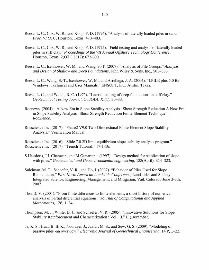
140
Reese, L. C., Cox, W. R., and Koop, F. D. (1974). “Analysis of laterally loaded piles in sand.”
Proc. VI OTC, Houston, Texas, 473–483.
Reese, L. C., Cox, W. R., and Koop, F. D. (1975). “Field testing and analysis of laterally loaded
piles in stiff clay.” Proceedings of the VII Annual Offshore Technology Conference,
Houston, Texas, 2(OTC 2312): 672-690.
Reese, L. C., Isenhower, W. M., and Wang, S.-T. (2007). “Analysis of Pile Groups.” Analysis
and Design of Shallow and Deep Foundations, John Wiley & Sons, Inc., 503–536.
Reese, L. C., Wang, S.-T., Isenhower, W. M., and Arrellaga, J. A. (2004). “LPILE plus 5.0 for
Windows, Technical and User Manuals.” ENSOFT, Inc., Austin, Texas.
Reese, L. C., and Welch, R. C. (1975). “Lateral loading of deep foundations in stiff clay.”
Geotechnical Testing Journal, GTJODJ, XI(1), 30–38.
Rocnews. (2004). “A New Era in Slope Stability Analysis : Shear Strength Reduction A New Era
in Slope Stability Analysis : Shear Strength Reduction Finite Element Technique.”
RocSience.
Rocscience Inc. (2017). “Phase2 V9.0 Two-Dimensional Finite Element Slope Stability
Analysis.” Verification Manual.
Rocscience Inc. (2016). “Slide 7.0 2D limit equilibrium slope stability analysis program.”
Rocscience Inc. (2017). “Trench Tutorial.” 17-1-16.
S.Hassiotis, J.L.Chamean, and M.Gunaratne. (1997). “Design method for stablization of slope
with piles.” Geotechnical and Geoenvironmental engineering, 123(April), 314–323.
Suleiman, M. T., Schaefer, V. R., and Ho, I. (2007). “Behavior of Piles Used for Slope
Remediation.” First North American Landslide Conference, Landslides and Society:
Integrated Science, Engineering, Management, and Mitigation, Vail, Colorado June 3-8th,
2007.
Thomã, V. (2001). “From finite diferences to finite elements; a short history of numerical
analysis of partial diferential equations.” Journal of Computational and Applied
Mathematics, 128, 1–54.
Thompson, M. J., White, D. J., and Schaefer, V. R. (2005). “Innovative Solutions for Slope
Stability Reinforcement and Characterization : Vol . II.” II (December).
Ti, K. S., Huat, B. B. K., Noorzaei, J., Jaafar, M. S., and Sew, G. S. (2009). “Modeling of
passive piles -an overview.” Electronic Journal of Geotechnical Engineering, 14 P, 1–22.

141
Turner, A. K., and Schuster, R. L. (1996). Landslides investigation and mitigation. (E. A. Keith
Turner, Robert L. Schuster, ed.), Transportation Research Board, Special report 247,
Washington, D.C.
USACE. (1995). Geotechnical Analisys by the Finite Element Method. Washington, DC.
Varnes, D. J. (1978). Slope Movements types and Processes. Chapter 2. Landslides: Analysis
and Control, Special Report, Transportation Research Board, Nacional Academy of
Sciences, Washington, D.C.
Vessely, A., Yamasaki, K., and Strom, R. (2007). “Landslide stabilization using piles.” 1st North
American Landslide Conference, V. R. Schaefer, R. L. Schuster, and A. K. Turner, eds.,
Omnipress, Vail, Colorado June 3-8th, 2007., 1–11.
Viggiani, C. (1981). “Ultimate lateral load on piles used to stabilzed landslides.” 10th In
ternational Conference on Soil Mechanics and Foundation Engineering, Stockolm, Vol. 3,
pp 555-560.
Whittle, A. J. (1999). “Role of finite element methods in geotechnical engineering.” BSCES
Journal of Civil Engineering Practice, 14(2), 81–88.
Won, J., You, K., Jeong, S., and Kim, S. (2005). “Coupled effects in stability analysis of pile-
slope systems.” Computers and Geotechnics, 32(4), 304–315.
Zhang, G., and Wang, L. (2010). “Stability analyis of strain-softening slope reinforced with
stabilizing piles.” Journal of Geotechnical and Geoenvironmental Engineering, 136(11),
1578–1588.
Zicko, K. E., Fleming, G., Hill, C., Lewis, P. J., Fleming, G., Hill, C., Hackenberg, E. A.,
Fleming, G., and Hill, C. (2011). “Slope Stabilization of Mill Creek Landslide Using Steel
H-Piles.” Deep Foundation Magazine, (May), 43–52.
Zienkiewicz, O., Humpheson, C., and Lewis, R. (1975). “Associated and nonassociated
viscoplasticity in soil mechanics.” Géotechnique, 25(4), 671–89.
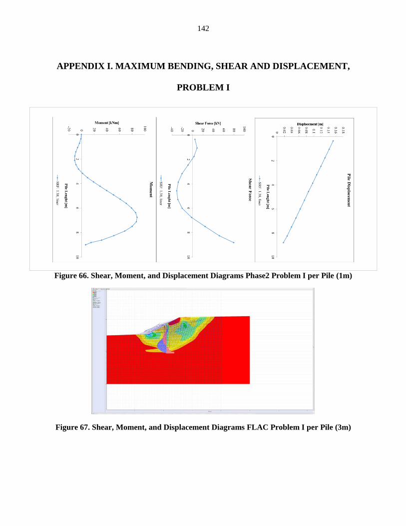
142
APPENDIX I. MAXIMUM BENDING, SHEAR AND DISPLACEMENT,
PROBLEM I
Figure 66. Shear, Moment, and Displacement Diagrams Phase2 Problem I per Pile (1m)
Figure 67. Shear, Moment, and Displacement Diagrams FLAC Problem I per Pile (3m)

143
APPENDIX II. NOMINAL BENDING AND SHEAR STRENGTH MILL
CREEK LANDSLIDE
The properties of the reduced section are presented in Figure 63. The nominal
parameters were calculated by following American Institute of Steel Construction (2016) for
non-compact section suggested to shear and flexural stresses as follows:
The Manual of Steel Construction by American Institute of Steel Construction (2016)
requires that steel structures and structural elements be design so that the strength limit state is
not exceeded when subjected to all required factored load combinations. For the strength limit
state, axial, flexural, shear strength are investigated.
Bending strength
In flexure design, the basic requirement is expressed as:
For LRFD design
𝑴𝒖 ≤ ∅𝑴𝒏 = 𝑴𝒓
For ASD design
𝑴𝒖 ≤𝑴𝒏
Ω= 𝑴𝒂
𝑀𝑢 𝑖𝑠 𝑡ℎ𝑒 𝑓𝑎𝑐𝑡𝑜𝑟𝑒𝑑 𝑚𝑜𝑚𝑒𝑛𝑡 𝑜𝑓 𝑡ℎ𝑒 𝑠𝑒𝑐𝑡𝑖𝑜𝑛 𝑎𝑛𝑑 𝑀𝑟 𝑖𝑠 𝑡ℎ𝑒 𝑓𝑎𝑐𝑡𝑜𝑟𝑒𝑑 𝑓𝑙𝑒𝑥𝑢𝑟𝑎𝑙 𝑟𝑒𝑠𝑖𝑠𝑡𝑎𝑛𝑐𝑒
𝑀𝑢 𝑖𝑠 𝑡ℎ𝑒 𝑚𝑜𝑚𝑒𝑛𝑡 𝑜𝑓 𝑡ℎ𝑒 𝑠𝑒𝑐𝑡𝑖𝑜𝑛 𝑎𝑛𝑑 𝑀𝑎 𝑖𝑠 𝑡ℎ𝑒 𝑎𝑙𝑙𝑜𝑎𝑏𝑙𝑒 𝑓𝑙𝑒𝑥𝑢𝑟𝑎𝑙 𝑟𝑒𝑠𝑖𝑠𝑡𝑎𝑛𝑐𝑒
LRFD resistance factor =0.90 ASD factor of safety=1.67

144
Because the HP section that have been analyzed is a non-compact section the nominal
moment strength should be the smallest value between lateral torsional buckling and the limit
state of yielding. However, because no axial compression load takes place and the bending
moment is considered to occur about the strong axis and loaded at the symmetry plane, the
nominal moment strength of the section will be:
𝑴𝒏 = 𝒇𝒚𝑺𝒙
𝑴𝒏 = 𝟓𝟎𝒌𝒔𝒊(𝟒𝟔. 𝟕𝟗𝟖) = 𝟐, 𝟑𝟒𝟎 𝒌𝒊𝒑𝒔 − 𝒊𝒏
Where 𝑓𝑦 the yield is stress of the section and 𝑆𝑥 is the elastic modulus of the section in in3.
Hence, the factored flexural resistance will be:
𝑀𝑟 = (𝟎. 𝟗) 𝟐, 𝟑𝟒𝟎 = 𝟐𝟏𝟎𝟔 𝒌𝒊𝒑𝒔 − 𝒊𝒏,
And the allowable bending moment;
𝑀𝑟 =𝟐𝟑𝟒𝟎
𝟏. 𝟔𝟕= 𝟏, 𝟒𝟎𝟏 𝒌𝒊𝒑𝒔 − 𝒊𝒏
Shear strength
As in the bending case, the design shear strength, ∅𝑽𝒏, and the allowable shear
strength,𝑽𝒏
Ω, will be found from determining the nominal shear strength as follows for I-
shaped members and channels:
LRFD resistance factor =0.90 ASD factor of safety=1.5
𝑉𝑛 = 0.6𝑓𝑦𝐴𝑤𝐶𝑣𝑤
𝑉𝑛 = 0.6(50𝑘𝑠𝑖)(11.66 𝑖𝑛𝑥0.31 𝑖𝑛)(1) = 108.4𝑘𝑖𝑝𝑠
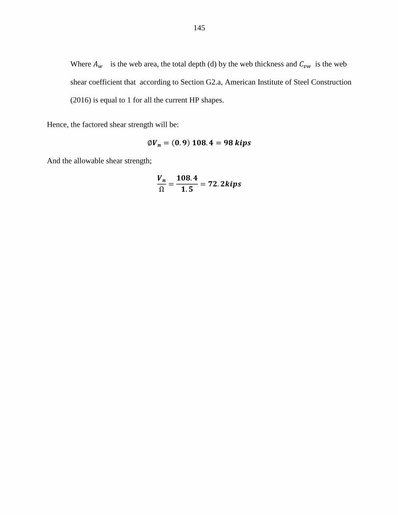
145
Where 𝐴𝑤 is the web area, the total depth (d) by the web thickness and 𝐶𝑣𝑤 is the web
shear coefficient that according to Section G2.a, American Institute of Steel Construction
(2016) is equal to 1 for all the current HP shapes.
Hence, the factored shear strength will be:
∅𝑽𝒏 = (𝟎. 𝟗) 𝟏𝟎𝟖. 𝟒 = 𝟗𝟖 𝒌𝒊𝒑𝒔
And the allowable shear strength;
𝑽𝒏Ω=𝟏𝟎𝟖. 𝟒
𝟏. 𝟓= 𝟕𝟐. 𝟐𝒌𝒊𝒑𝒔

146
Figure 68. Geometry and properties reduced HP12x53 section from SAP200 v 18.1.1 by
CSI (2016)