Comparison of continuous and discrete-timedata-based modeling for hypoelliptic systems

Fei Lu∗, Kevin K. Lin†, and Alexandre J. Chorin∗

Abstract

We compare two approaches to the predictive modeling of dynamical systems frompartial observations at discrete times. The first is continuous in time, where one usesdata to infer a model in the form of stochastic differential equations, which are thendiscretized for numerical solution. The second is discrete in time, where one directlyinfers a discrete-time model in the form of a nonlinear autoregression moving averagemodel. The comparison is performed in a special case where the observations areknown to have been obtained from a hypoelliptic stochastic differential equation. Weshow that the discrete-time approach has better predictive skills, especially when thedata are relatively sparse in time. We discuss open questions as well as the broadersignificance of the results.

Keywords: Hypoellipticity; stochastic parametrization; Kramers oscillator; statisticalinference; discrete partial data; NARMA.

1 Introduction

We examine the problem of inferring predictive stochastic models for a dynamical system,given partial observations of the system at a discrete sequence of times. This inferenceproblem arises in applications ranging from molecular dynamics to climate modeling (see,e.g. [10, 12] and references therein). The observations may come from a stochastic or adeterministic chaotic system. This inference process, often called stochastic parametrization,is useful both for reducing computational cost by constructing effective lower-dimensionalmodels, and for making prediction possible when fully-resolved measurements of initial dataand/or a full model are not available.

Typical approaches to stochastic parametrization begin by identifying a continuous-timemodel, usually in the form of stochastic differential equations (SDEs), then discretizing theresulting model to make predictions. One difficulty with this standard approach is that itoften leads to hypoelliptic systems [19, 22, 28], in which the noise acts on a proper subset ofstate space directions. As we will explain, this degeneracy can make parameter estimationfor hypoelliptic systems particularly difficult [28,30,33], makiing the resulting model a poorpredictor for the system at hand.

∗Department of Mathematics, University of California, Berkeley and Lawrence Berkeley National Labo-ratory. E-mail addresses: feilu@berkeley.edu (FL); chorin@math.berkeley.edu (AC)†School of Mathematical Sciences, University of Arizona. E-mail address: klin@math.arizona.edu

1

Recent work [8,21] has shown that fully discrete-time approaches to stochastic parametriza-tion, in which one considers a discrete-time parametric model and infers its parameters fromdata, have certain advantages over continuous-time methods. In this paper, we comparethe standard, continuous-time approach with a fully discrete-time approach, in a special casewhere the observations are known in advance to have been produced by a hypoelliptic systemwhose form is known, and only some parameters remain to be inferred. We hope that thiscomparison, in a relatively simple and well-understood context, will clarify some of the ad-vantages and disadvantages of discrete-time modeling for dynamical systems. We note thatour discussion here leaves in abeyance the question of what to do in cases where much lessis known about the origin of the data; in general, there is no reason to believe that a givenset of observations was generated by any stochastic differential equation or by a Markovianmodel of any kind.

A major difficulty in discrete modeling is the derivation of the structure, i.e. of the termsin the discrete-time model. We show that when the form of the differential equation givingrise to the data is known, one can deduce possible terms for the discrete model, but notnecessarily the associated coefficients, from numerical schemes. Note that the use of thisidea places the discrete and continuous models we compare on an equal footing, in that bothapproaches produce models directly derived from the assumed form of the model.

Model and goals. The specific hypoelliptic stochastic differential equations we work withhave the form

dxt = yt dt, (1.1)

dyt =(− γyt − V ′(xt)

)dt+ σdBt ,

where Bt is a standard Wiener process. When the potential V is quadratic, i.e.,

V (x) =α

2x2 , α > 0,

we get a linear Langevin equation. When the potential has the form

V (x) =β

4x4 − α

2x2 , α, β > 0,

this is the Kramers oscillator [3,15,20,31]. It describes the motion of a particle in a double-well potential driven by white noise, with xt and yt being the position and the velocityof the particle; γ > 0 is a damping constant. The white noise represents the thermalfluctuations of a surrounding “heat bath”, the temperature of which is connected to γand σ via the Einstein relation T = σ2

2γ. This system is ergodic, with stationary density

p(x, y) ∝ exp(− 2γσ2

(12y2 + V (x)

)). It has multiple time scales and can be highly nonlinear,

but is simple enough to permit detailed numerical study. Parameter estimation for this sys-tem is also rather well-studied [28, 30]. These properties make Eq. (1.1) a natural examplefor this paper.

One of our goals is to construct a model that can make short-time forecasts of the evolutionof the variable x based on past observations {xnh}Nn=1, where h > 0 is the observation spacing,in the situation where the parameters γ, α, β, and σ are unknown. (The variable y is notobserved, hence even when the parameters are known, the initial value of y is missing whenone tries to solve the SDEs to make predictions.) We also require that the constructedmodel be able to reproduce long-term statistics of the data, e.g., marginals of the stationarydistribution. In part, this is because the form of the model (either continuous or discrete-time)

2

is generally unknown, and reproduction of long-term statistics provides a useful criterion forselecting a particular model. But even more important, in order for a model to be useful fortasks like data assimilation and uncertainty quantification, it must faithfully capture relevantstatistics on time scales ranging from the short term (on which trajectory-wise forecasting ispossible) to longer time scales.

Our main finding is that the discrete-time approach makes predictions as reliably asthe true system that gave rise to the data (which is of course unknown in general), even forrelatively large observation spacings, while a continuous-time approach is only accurate whenthe observation spacing h is small, even in very low-dimensional examples such as ours.

Paper organization. We briefly review some basic facts about hypoelliptic systems in Sec-tion 2, including the parameter estimation technique we use to implement the continuous-timeapproach. In Section 3, we discuss the discrete-time approach. Section 4 presents numericalresults, and in Section 5 we summarize our findings and discuss broader implications of ourresults. For the convenience of the reader, we collect a number of standard results aboutSDEs and their numerical solutions in the Appendices.

2 Brief review of the continuous-time approach

2.1 Inference for partially observed hypoelliptic systems

Consider a stochastic differential equation of the form

dX = f(X, Y ) dtdY = a(X, Y ) dt+ b(X, Y ) dWt .

(2.1)

Observe that only the Y equation is stochastically forced. Because of this, the second-orderoperator in the Fokker-Planck equation

∂

∂tp(x, y, t) = − ∂

∂x[f(x, y)p(x, y, t)]− ∂

∂y[a(x, y)p(x, y, t)] +

1

2

∂2

∂y2[b2(x, y)p(x, y, t)] (2.2)

for the time evolution of probability densities is not elliptic. This means that without anyfurther assumptions on Eq. (2.1), the solutions of the Fokker-Planck equation, and hencethe transition probability associated with the SDE, might be singular in the X direction.Hypoellipticity is a condition that guarantees the existence of smooth solutions for Eq. (2.2)despite this degeneracy. Roughly speaking, a system is hypoelliptic if the drift terms (i.e.,the vector fields f(x, y) and a(x, y)) help to spread the noise to all phase space directions,so that the system has a nondegenerate transition density. Technically, hypoellipticity re-quires certain conditions involving the Lie brackets of drift and diffusion fields, known asHormander’s conditions [26]; when these conditions are satisfied, the system can be shownto possess smooth transition densities.

Our interest is in systems for which only discrete observations of x are available, and weuse these observations to estimate the parameters in the functions f, a, b. While parameterestimation for completely observed nondegenerate systems has been widely investigated (seee.g. [29, 33]), and there has been recent progress toward parameter estimation for partially-observed nondegenerate systems [16], parameter estimation from discrete partial observationsfor hypoelliptic systems remains challenging.

There are three main categories of methods for parameter estimation (see, e.g., the surveys[32], and [33]):

3

(i) Likelihood-type methods, where the likelihood is analytically or numerically approx-imated, or a likelihood-type function is constructed based on approximate equations.These methods lead to maximum likelihood estimators (MLE).

(ii) Bayesian methods, in which one combines a prior with a likelihood, and one uses theposterior mean as estimator. Bayesian methods are important when the likelihood hasmultiple maxima. However, suitable priors may not always be available.

(iii) Estimating function methods, or generalized moments methods, where estimators arefound by estimating functions of parameters and observations. These methods gen-eralize likelihood-type methods, and are useful when transition densities (and hencelikelihoods) are difficult to compute. Estimating functions can be constructed usingassociated martingales or moments.

Because projections of Markov processes are typically not Markov, and the system is hypoel-liptic, all three of the above approaches face difficulties for systems like (1.1): the likelihoodfunction is difficult to compute either analytically or numerically, because only partial ob-servations are available, and likelihood-type functions based on approximate equations oftenlead to biased estimators [11,28,30]. There are also no easily calculated martingales on whichto base estimating functions [9].

There are two special cases that have been well-studied. When the system is linear, theobserved process is a continuous-time autoregression process. Parameter estimation for thiscase is well-understood, see, e.g., the review papers [5, 7]. When the observations constitutean integrated diffusion (that is, f(x, y) = y and the Y equation is autonomous, so that Xis an integral of the diffusion process Y ), consistent, asymptotically normal estimators areconstructed in [9] using prediction-based estimating functions, and in [11] using a likelihoodtype method based on Euler approximation. However, these approaches rely on the systembeing linear or the unobserved process being autonomous, and are not adapted to generalhypoelliptic systems.

To our knowledge, for general hypoelliptic systems with discrete partial observation, onlyBayesian type methods [28] and a likelihood type method [30] have been proposed whenf(x, y) is such that Eq. (2.1) can be written in the form of Eq. (1.1) by a change of variables.In [28] Euler and Ito-Taylor approximations are combined in a deterministic scan Gibbssampler alternating between parameters and missing data in the unobserved variables. Thereason for combining Euler and Ito-Taylor approximation is that Euler approximation leadsto underestimated MLE of diffusion but is effective for drift estimation, whereas Ito-Taylorexpansion leads to unbiased MLE of diffusion but is inappropriate for drift estimation. In [30]explicit consistent maximum likelihood-type estimators are constructed. However, all thesemethods require the observation spacing h to be small and the number of observations N tobe large. For example, the estimators in [30] are only guaranteed to converge if, as N →∞,h → 0 in such a way that Nh2 → 0 and Nh → ∞. In practice, the observation spacingh > 0 is fixed, and large biases have been observed when h is not sufficiently small [28, 30].We show in this paper that the bias can be so large that the prediction from the estimatedsystem may be unreliable.

2.2 Continuous-time stochastic parametrization

The continuous-time approach starts by proposing a parametric hypoelliptic system andestimating parameters in the system from discrete partial observations. In the present paper,the form of the hypoelliptic system is assumed to be known. Based on the Euler scheme

4

approximation of the second equation in the system, Samson and Thieullen [30] constructedthe following likelihood-type function, or “contrast”

LN(θ) =N−3∑n=1

3

2

[y(n+2)h − y(n+1)h + h(γynh + V ′(xnh))

]2hσ2

+ (N − 3) log σ2,

where θ = (γ, β, α, σ2) and

yn =x(n+1)h − xnh

h. (2.3)

Note that a shift in time in the drift term, i.e. the time index of γynh + V ′(xnh) is nhinstead of (n + 1)h, is introduced to avoid a

√h correlation between y(n+2)h − y(n+1)h and

γy(n+1)h + V ′(x(n+1)h). Note also that there is a weighting factor 32

in the sum, because themaximum likelihood estimator based on Euler approximation underestimates the variance(see, e.g., [11, 28]).

The estimator is the minimizer of the contrast

θN = arg minθLN(θ). (2.4)

The estimator θN converges to the true parameter value θ = (γ, β, α, σ2) under the conditionthat h→ 0, Nh→∞ and Nh2 → 0. However, if h is not small enough, the estimator θN canhave a large bias (see in [30] and in the later sections), and the bias can be so large that theestimated system may have dynamics very different from the true system, and its predictionbecomes unreliable.

Remark 2.1 In the case V ′(x) = αx, the Langevin system (1.1) is linear. The process{xt, t ≥ 0} is a continuous-time autoregressive process of order two, and there are variousways to estimate the parameters (see the review [6]), e.g., the likelihood method using a state-space representation and a Kalman recursion [17], or methods for fitting discrete-time ARMAmodels [27]. However, none of these approaches can be extended to nonlinear Langevinsystems. In this section we focus on methods that work for nonlinear systems.

Once the parameters have been estimated, one numerically solves the estimated systemto make predictions. In this paper, to make predictions for time t > Nh (where N isthe number of observations), we use the initial condition (xNh, yN) in solving the estimatedsystem, with yN being an estimate of yNh based on observations x. Since the system isstochastic, we use an “ensemble forecasting” method to make predictions. We start a numberof trajectories from the same initial condition, and evolve each member of this ensembleindependently. The ensemble characterizes the possible motions of the particle conditionalon past observations, and the ensemble mean provides a specific prediction. For the purposeof short-term prediction, the estimated system can be solved with small time steps, hence alow order scheme such as the Euler scheme may be used.

However, in many practical applications, the true system is unknown [8,21], and one has tovalidate the continuous-time model by its ability to reproduce the long-term statistics of data.For this purpose, one has to compute the ergodic limits of the estimated system. The Eulerscheme may be numerically unstable when the system is not globally Lipschitz, and a betterscheme such as implicit Euler (see e.g. [23, 24, 34]) or the quasi-symplectic integrator [25], isneeded. In our study, the Euler scheme is numerically unstable, while the Ito-Taylor schemeof strong order 2.0 in (C.2) produces long-term statistics close to those produced by theimplicit Euler scheme. We use the Ito-Taylor scheme, since it has the advantage of beingexplicit and was used in [28].

5

In summary, the continuous-time approach uses the following algorithm to generate aforecasting ensemble of trajectories.

Algorithm 2.1 (Continuous-time approach) With data {xnh}Nn=1,Step 1. Estimate the parameters using (2.4);Step 2. Select a numerical scheme for the SDE, e.g. the Ito-Taylor scheme in the

appendix;Step 3. Solve the SDE (1.1) with estimated parameters, using small time steps dt and

initial data(xNh,

xNh−xNh−hh

), to generate the forecasting ensemble.

3 The discrete-time approach

3.1 NARMA representation

In the discrete-time approach, the goal is to infer a discrete-time predictive model for xfrom the data. Following [8], we choose a discrete-time system in the form of a nonlinearautoregression moving average (NARMA) model of the following form:

Xn = Φn + ξn, (3.1)

Φn :=µ+

p∑j=1

ajXn−j +r∑

k=1

bkQk(Xn−p:n−1, ξn−q:n−1) +

q∑j=1

cjξn−j, (3.2)

where p is the order of the autoregression, q is the order of the moving average, and the Qk

are given nonlinear functions (see below) of (Xn−p:n−1, ξn−q:n−1). Here {ξn} is a sequence ofi.i.d Gaussian random variables with mean zero and variance c2

0 (denoted by N (0, c20)). The

numbers p, q, r, as well as the coefficients aj, bj, and cj are to be determined from data.A main challenge in designing NARMA models is the choice of the functions Qk, a process

we call “structure selection” or “structure derivation”. Good structure design leads to modelsthat fit data well and have good predictive capabilities. Using too many unnecessary terms,on the other hand, can lead to overfitting or inefficiency, while too few terms can lead to anineffective model. As before, we assume that a parametric family containing the true modelis known, and we show that suitable structures for NARMA can be derived from numericalschemes for solving SDEs. We propose the following practical criteria for structure selection:(i) the model should be numerically stable; (ii) we select the model that makes the bestpredictions (in practice, the predictions can be tested using the given data.); (iii) the large-time statistics of the model should agree with those of the data. These criteria are notsufficient to uniquely specify a viable model, and we shall return to this issue when wediscuss the numerical experiments.

Once the Qk have been chosen, the coefficients (aj, bj, cj) are estimated from data usingthe following conditional likelihood method. Conditional on ξ1, . . . , ξm, the log-likelihood of{Xn = xnh}Nn=m+1 is

LN(ϑ|ξ1, . . . , ξm) =N∑

n=m+1

(Xn − Φn)2

2c20

+N − q

2log c2

0, (3.3)

where m = max{p, q} and ϑ = (aj, bj, cj, c20), and Φn is defined in Eq. (3.2). The log-

likelihood is computed as follows. Conditionally on given values of {ξ1, . . . , ξm}, one cancompute Φm+1 from data {Xn = xnh}mn=1 using Eq. (3.2). With the value of ξm+1 followingfrom (3.1), one can then compute Φm+2. Repeating this recursive procedure, one obtains the

6

values of {Φn}Nn=m+1 that are needed to evaluate the log-likelihood. The estimator of theparameter ϑ = (aj, bj, cj, c

20) is the minimizer of the log-likelihood

ϑN = arg minϑLN(ϑ|ξ1, . . . , ξm).

If the system is ergodic, the conditional maximum likelihood estimator ϑN can be provedto be consistent (see e.g. [1, 13]), which means that it converges almost surely to the trueparameter value as N →∞. Note that the estimator requires the values of ξ1, · · · , ξm, whichis in general not available. But ergodicity implies that if N is large, ϑN forgets about thevalues of ξ1, · · · , ξm quickly anyway, and in practice, we can simply set ξ1 = · · · = ξm = 0.Also, in practice, we initialize the optimization with c1 = · · · = cq = 0 and with the valuesof (aj, bj) computed by least-squares.

Note that in the case q = 0, the estimator is the same as the nonlinear least-squares esti-mator. The noise sequence {ξn} does not have to be Gaussian for the conditional likelihoodmethod to work, so long as the expression in Eq. (3.3) is adjusted accordingly.

In summary, the discrete-time approach uses the following algorithm to a generate aforecasting ensemble.

Algorithm 3.1 (Discrete-time approach) With data {xnh}Nn=1,Step 1. Find possible structures for NARMA;Step 2. Estimate the parameters in NARMA for each possible structure;Step 3. Select the structure that fits the data best, in the sense that it reproduces best

the long-term statistics and makes the best predictions;Step 4. Use the resulting model to generate a forecasting ensemble.

3.2 Structure derivation for the linear Langevin equation

The main difficulty in the discrete-time approach is the derivation of the structure of theNARMA model. In this section we discuss how to derive this structure from the SDEs, firstin the linear case.

For the linear Langevin equation, the discrete-time system should be linear. Hence weset r = 0 in (3.1) and obtain an ARMA(p, q) model. The linear Langevin equation{

dx = ydt,

dy = (−γy − αx)dt+ σdBt,(3.4)

can be solved analytically. The solution xt at discrete times satisfies (see Appendix A)

x(n+2)h = a1x(n+1)h + a2xnh − a22Wn+1,1 +Wn+2,1 + a12Wn+1,2, (3.5)

where {Wn,i} are defined in (A.1), and

a1 = trace(eAh), a2 = −e−γh, aij =(eAh)ij, for A =

(0 1−α−γ

). (3.6)

The process {xnh} defined in Eq. (3.5) is, strictly speaking, not an ARMA process (seeAppendix B for all relevant, standard definitions used in this section), because {Wn,1}∞n=1

and {Wn,2}∞n=1 are not linearly dependent and would require at least two independent noisesequences to represent, while an ARMA process requires only one. However, as the followingproposition shows, there is an ARMA process with the same distribution as the process{xnh}. Since the minimum mean-square-error state predictor of a stationary Gaussian processdepends only on its autocovariance function (see, e.g., [4, Chapter 5]), an ARMA processequal in distribution to the discrete-time Langevin equation is what we need here.

7

Proposition 3.2 The ARMA(2, 1) process

Xn+2 = a1Xn+1 + a2Xn +Wn + θ1Wn−1, (3.7)

where a1, a2 are given in (3.6) and the {Wn} are i.i.d N (0, σ2W ), is the unique process in

the family of invertible ARMA processes that has the same distribution as the process {xnh}.Here σ2

W and θ1 (θ1 < 1 so that the process is invertible) satisfy the equations

σ2W

(1 + θ2

1 + θ1a1

)= γ0 − γ1a1 − γ2a2,

σ2W θ1 = γ1 (1− a2)− γ0a1,

where {γj}2j=0 are the autocovariances of the process {xnh} and are given in Lemma A.1.

Proof. Since the stationary process {xnh} is a centered Gaussian process, we only need to findan ARMA(p, q) process with the same autocovariance function as {xnh}. The autocovariancefunction of {xnh}, denoted by {γn}∞n=0, is given by (see Lemma A.1)

γn = γ0 ×

{1

λ1−λ2 (λ1eλ2nh − λ2e

λ1nh), if γ2 − 4α 6= 0;

eλ0nh(1− λ0nh), if γ2 − 4α = 0,

where (λ1, λ2, or λ0) are the roots of the characteristic polynomial λ2 + γλ + α = 0 of thematrix A in (3.6).

On the other hand, the autocovariance function of an ARMA(p, q) process

Xn − φ1Xn−1 − · · · − φpXn−p = Wn + θ1Wn−1 + · · ·+ θqWn−q,

denoted as {γ (n)}∞n=0, is given by (see Eq. (B.4))

γ(n) =k∑i=1

ri−1∑j=0

βijnjζ−ni , for n ≥ max{p, q + 1} − p,

where (ζi, i = 1, . . . , k) are the distinct zeros of φ(z) := 1 − φ1z − · · · − φpzp, and ri is the

multiplicity of ζi (hence∑k

i=1 ri = p), and {βij} are constants.Since {γn}∞n=0 only provides two possible roots, ζi = e−λih or ζi = e−λ0h for i = 1, 2, the

order p must be that p = 2. From these two roots, one can compute the coefficients φ1 andφ2 in the ARMA(2, q) process:

φ1 = ζ−11 + ζ−1

2 = trace(eAh) = a1, φ2 = −ζ−11 ζ−1

2 = −e−γh = a2.

Since γk − φ1γk−1 − φ2γk−2 = 0 for any k ≥ 2, we have q ≤ 1. Since γ1 − φ1γ0 − φ2γ1 6= 0,Example B.2 indicates that q 6= 0. Hence q = 1 and the above ARMA(2, 1) is the uniqueprocess in the family of invertible ARMA(p, q) processes that has the same distribution as{xnh}. The equations for σ2

W and θ1 follow from Example B.3.

This proposition indicates that the discrete-time system for the linear Langevin systemshould be an ARMA(2, 1) model.

Example 3.3 Suppose ∆ := γ2 − 4α < 0. Then the parameters in the ARMA(2, 1) process

(3.7) are given by a1 = 2e−γ2h cos(

√−∆2h), a2 = −e−γh and

θ1 =c− a1 −

√(c− a1)2 − 4

2, σ2

w =γ1(1− a2)− γ0a1

θ1

.

where c = γ0−γ1a1−γ2a2γ1(1−a2)−γ0a1 , and γn = σ2

2γα

(cos(

√−∆2nh) + γ√

−∆sin(

√−∆2nh))

for n ≥ 0.

8

Remark 3.4 The maximum likelihood estimators of ARMA parameters can also be com-puted using a state-space representation and a Kalman recursion (see e.g. [4]). This approachis essentially the same as the conditional likelihood method in our discrete-time approach.

Remark 3.5 The proposition indicates that the parameters in the linear Langevin equationcan also be computed from the ARMA(2, 1) estimators, because from the proof we have

γ = − ln(−a2)h

= −λ1 − λ2, α = λ1λ2, and σ2 = 2γασ2W , where (λi, i = 1, 2) satisfies that

(e−λih, i = 1, 2) are the two roots of φ(z) = 1− a1z − a2z.

3.3 Structure derivation for the Kramers oscillator

For nonlinear Langevin systems, in general there is no analytical solution, so the approachof Section 3.2 cannot be used. Instead, we derive structures from the numerical schemes forsolving stochastic differential equations. For simplicity, we choose to focus on explicit termsin a discrete-time system, so implicit schemes (in e.g. [23, 25, 34]) are not suitable. Here wefocus on deriving structures from two explicit schemes: the Euler–Maruyama scheme andthe Ito-Taylor scheme of order 2.0; see Appendix C for a brief review of these schemes. Asmentioned before, we expect our approach to extend to other explicit schemes, e.g., thatof [2]. While we consider specifically Eq. (1.1), the method used in this section extends tosituations when f(x, y) is such that Eq. (2.1) can be rewritten in form Eq. (1.1) and itshigher-dimensional analogs by a change of variables.

As warm-up, we begin with the Euler–Maruyama scheme. Applying this scheme (C.1) tothe system (1.1), we find:

xn+1 =xn + ynh,

yn+1 = yn(1− γh)− hV ′(xn) +Wn+1,

where Wn = σh1/2ζn, with {ζn} is an i.id. sequence of N (0, 1) random variables. Straight-forward substitutions yield a closed system for x

xn = (2− γh)xn−1 − (1− γh)xn−2 − h2V ′(xn−2) + hWn−1.

Since V ′(x) = βx3 − αx, this leads to the following possible structure for NARMA:Model (M1):

Xn = a1Xn−1 + a2Xn−2 + b1X3n−2 + ξn +

q∑j=1

cjξn−j + µ. (3.8)

Next, we derive a structure from the Ito-Taylor scheme of order 2.0. Applying the scheme(C.2) to the system (1.1), we find

xn+1 =xn + h (1− 0.5γh) yn − 0.5h2V ′ (xn) + Zn+1,

yn+1 = yn[1− γh+ 0.5γ2h2 − 0.5h2V ′′ (xn)

]− h (1− 0.5γh)V ′ (xn) +Wn+1 − γZn+1,

where Zn = σh3/2(ζn + ηn/

√3), with {ηn} being an i.id. N (0, 1) sequence independent of

{ζn}. Straightforward substitutions yield a closed system for x :

xn =xn−1

[2− γh+ 0.5γ2h2 − h2V ′′ (xn−2)

]− 0.5h2V ′ (xn−1) + Zn

+[1− γh+ 0.5γ2h2 − 0.5h2V ′′ (xn−2)

] (−xn−2 + 0.5h2V ′ (xn−2)− Zn−1

)−h2 (1− 0.5γh)2 V ′ (xn−2) + h (1− 0.5γh) (Wn−1 − γZn−1) .

9

Note that Wn is of order h1/2 and Zn is of order h3/2. Writing the terms in descending order,we obtain

xn =(2− γh+ 0.5γ2h2

)xn−1 −

(1− γh+ 0.5γ2h2

)xn−2 (3.9)

+Zn − Zn−1 + h (1− 0.5γh)Wn−1 − 0.5h2V ′ (xn−1) + 0.5h2V ′′ (xn−2) (xn−1 − xn−2)

+0.5γh3V ′ (xn−2) + 0.5h2V ′′ (xn−2)Zn−1 − 0.5h4V ′′ (xn−2)V ′ (xn−2) .

This equation suggests that p = 2 and q = 0 or 1. The noise term Zn−Zn−1+h (1− 0.5γh)Wn−1

is of order h1.5, and involves two independent noise sequences {ζn} and {ηn}, hence the aboveequation for xn is not a NARMA model. However, it suggests possible structures for NARMAmodels. In comparison to model (M1), the above equation has (i) different nonlinear termsof order h2: h2V ′ (xn−1) and h2V ′′ (xn−2) (xn−1 − xn−2); (ii) additional nonlinear terms oforders three and larger: h3V ′ (xn−2), h2Zn−1V

′′ (xn−2), and h4V ′′ (xn−2)V ′ (xn−2). It is notclear which terms should be used, and one may be tempted to include as many terms aspossible. However, this can lead to overfitting. Hence, we consider different structures bysuccessively adding more and more terms, and select the one that fits data the best. Usingthe fact that V ′(x) = βx3 − αx, these terms lead to the following possible structures forNARMA:Model (M2):

Xn = a1Xn−1 + a2Xn−2 + b1X3n−1 + b2X

2n−2 (Xn−1 −Xn−2)︸ ︷︷ ︸+ξn +

q∑j=1

cjξn−j + µ,

where b1 and b2 are of order h2, and q ≥ 0;Model (M3):

Xn = a1Xn−1 + a2Xn−2 + b1X3n−1 + b2X

2n−2 (Xn−1 −Xn−2)︸ ︷︷ ︸

+ b3X3n−2︸ ︷︷ ︸+ξn +

q∑j=1

cjξn−j + µ,

where b3 is of order h3, and q ≥ 0;Model (M4):

Xn = a1Xn−1 + a2Xn−2 + b1X3n−1 + b2X

2n−2Xn−1︸ ︷︷ ︸+ b3X

3n−2︸ ︷︷ ︸+ b4X

5n−2︸ ︷︷ ︸

+ b5X2n−2ξn−1︸ ︷︷ ︸+ξn +

q∑j=1

cjξn−j + µ,

where b4 is of order h4, and b5 is of order h3.5, and q ≥ 1. (For the reader’s convenience, wehave highlighted all higher-order terms derived from V ′(x).)

From the model (M2)–(M4), the number of nonlinear terms increases as their order in-creases in the numerical scheme. Following [8,21], we use only the form of the terms derivedfrom numerical analysis, and not their coefficients; we estimate new coefficients from data.

4 Numerical study

We test the continuous and discrete-time approaches for data sets with different observationintervals h. The data are generated by solving the general Langevin Eq. (1.1) using a second-order Ito-Taylor scheme, with a small step size dt = 1/1024, and making observations with

10

Table 1: Mean and standard deviation of the estimators of the parameters (γ, α, σ) of thelinear Langevin equation in the continuous-time approach, computed on 100 simulations.

Estimator True value h = 1/32 h = 1/16 h = 1/8γ 0.5 0.7313 (0.0106) 0.9538 (0.0104) 1.3493 (0.0098)α 4 3.8917 (0.0193) 3.7540 (0.0187) 3.3984 (0.0172)σ 1 0.9879 (0.0014) 0.9729 (0.0019) 0.9411 (0.0023)

time intervals h = 1/32, 1/16, and 1/8; the value of time step dt in the integration has beenchosen to be sufficiently small to guarantee reasonable accuracy. For each one of the datasets, we estimate the parameters in the SDE and in the NARMA models. We then comparethe estimated SDE and the NARMA model by their ability to reproduce long-term statisticsand to perform short-term prediction.

4.1 The linear Langevin equation

We first discuss numerical results in the linear case. Both approaches start by computingthe estimators. The estimator θ = (γ, α, σ) of the parameters (γ, α, σ) of the linear LangevinEq. (3.4) is given by

θ = arg minθ=(γ,α,σ)

[N−3∑n=1

3

2

[yn+2 − yn+1 + h(γyn + αxn)]2

hσ2+ (N − 3) log σ2

], (4.1)

where yn is computed from data using (2.3).Following Eq. (3.7), we use the ARMA(2, 1) model in the discrete-time approach:

Xn+2 = a1Xn+1 + a2Xn +Wn + θ1Wn−1,

We estimate the parameters a1, a2, θ1, and σ2W from data using the conditional likelihood

method of Section 3.1.First, we investigate the reliability of the estimators. A hundred simulated data sets

are generated from Eq. (3.4) with true parameters γ = 0.5, α = 4, and σ = 1, and withinitial condition x0 = y0 = 1

2and time interval [0, 104]. The estimators, of (γ, α, σ) in the

linear Langevin equation and of (a1, a2, θ1, σW ) in the ARMA(2, 1) model, are computed foreach data set. Empirical mean and standard deviation of the estimators are reported inTable 1 for the continuous-time approach, and Table 2 for the discrete-time approach. In thecontinuous-time approach, the biases of the estimators grow as h increases. In particular,large biases occur for the estimators of γ: the bias of γ increases from 0.2313 when h = 1/32to 0.4879 when h = 1/8, while the true value is γ = 0.5; similarly large biases were alsonoticed in [30]. In contrast, the biases are much smaller for the discrete-time approach. The“theoretical value” (denoted by “T-value”) of a1, a2 , θ1 and σ2

W are computed analyticallyas in Example 3.3. Table 2 shows that the estimators in the discrete-time approach havenegligible differences from the theoretical values.

In practice, the above test of the reliability of estimators cannot be performed, becauseone has only a single data set and the true system that generated the data is unknown.

We now compare the two approaches in a practical setting, by assuming that we areonly given a single data set from discrete observations of a long trajectory on time interval[0, T ] with T = 217 ≈ 1.31 × 105. We estimate the parameters in the SDE and the ARMAmodel, and again investigate the performance of the estimated SDE and ARMA model in

11

Table 2: Mean and standard deviation of the estimators of the parameters (a1, a2, θ1, σW )of the ARMA(2, 1) model in the discrete-time approach, computed on 100 simulations. Thetheoretical value (denoted by T-value) of the parameters are computed from proposition 3.2.

Estimator h = 1/32 h = 1/16 h = 1/8T-value Est. value T-value Est. value T-value Est. value

a1 1.9806 1.9807 (0.0003) 1.9539 1.9541 (0.0007) 1.8791 1.8796 (0.0014)−a2 0.9845 0.9846 (0.0003) 0.9692 0.9695 (0.0007) 0.9394 0.9399 (0.0014)

θ1 0.2681 0.2667 (0.0017) 0.2684 0.2680 (0.0025) 0.2698 0.2700 (0.0037)σW 0.0043 0.0043 (0.0000) 0.0121 0.0121 (0.0000) 0.0336 0.0336 (0.0001)

reproducing long-term statistics and in predicting the short-term evolution of x. The long-term statistics are computed by time-averaging. The first half of the data set is used tocompute the estimators, and the second half of the data set is used to test the prediction.

The long-term statistics, i.e., the empirical probability density function (PDF) and theautocorrelation function (ACF), are shown in Figure 1. For all the three values of h, theARMA models reproduce the empirical PDF and ACF almost perfectly. The estimated SDEsmiss the spread of the PDF and the amplitude of oscillation in the ACF, and these errorbecome larger as h increases.

Next, we use an ensemble of trajectories to predict the motion of x. For each ensemble,we calculate the mean trajectory and compare it with the true trajectory from the data. Wemeasure the performance of the prediction by computing the root-mean-square-error (RMSE)of a large number of ensembles as follows: take N0 short pieces of data from the second half of

the long trajectory, denoted by{(x(ni+1)h, . . . , x(ni+K)h

)}N0

i=1, where ni = Ki. For each short

piece of data(x(ni+1)h, . . . , x(ni+K)h

), we generate Nens trajectories

{(X i,j

1 , . . . , X i,jK

)}Nensj=1

using a prediction system (i.e., the NARMA(p, q), the estimated Langevin system, or thetrue Langevin system), starting all ensemble members from the same several-step initialcondition

(x(ni+1)h, . . . , x(ni+m)h

), where m = 2 max {p, q} + 1. For the NARMA(p, q) we

start with ξ1 = · · · = ξq = 0. For the estimated Langevin system and the true Langevin

system, we start with initial condition(x(ni+m)h, yni

)with yni =

x(ni+m)h−x(ni+m−1)h

hand solve

the equations using the Ito-Taylor scheme of order 2.0 with a time step dt = 1/64 and recordthe trajectories every h/dt steps to get the prediction trajectories

(X i,j

1 , . . . , X i,jK

).

We then calculate the mean trajectory for each ensemble, Xi

k = 1Nens

∑Nensj=1 X i,j

k , k =1, . . . , K. The RMSE measures, in an average sense, the difference between the mean ensem-ble trajectory and the true data trajectory:

RMSE(kh) :=

(1

N0

N0∑i=1

∣∣∣X i

k − x(ni+k)h

∣∣∣2)1/2

.

The RMSE measures the accuracy of the mean ensemble prediction; RMSE = 0 correspondsto a perfect prediction, and small RMSEs are desired.

The computed RMSEs for N0 = 104 ensembles with Nens = 20 are shown in Figure 2.The ARMA(2, 1) model reproduces almost exactly the RMSEs of the true system for allthree observation step-sizes, while the estimated system has RMSEs deviating from that ofthe true system as h increases. The estimated system has smaller RMSEs than the truesystem, because it underestimates the variance of the true process xt (that is, σ2

2αγ< σ2

2αγ)

and because the means of xt decay exponential to zero. The steady increase in RMSE,

12

-2 -1 0 1 2x

0

0.2

0.4

0.6

0.8

1

1.2PD

FDataARMAEst. SDE

-2 -1 0 1 2x

DataARMAEst. SDE

-2 -1 0 1 2x

DataARMAEst. SDE

0 5 10time

-0.5

0

0.5

1

ACF

DataARMAEst. SDE

0 5 10time

DataARMAEst. SDE

0 5 10time

DataARMAEst. SDE

Figure 1: Empirical PDF and ACF of the ARMA(2, 1) models and the estimated linearLangevin system (denoted by Est. SDE), in the cases h = 1/32 (left column), h = 1/16(middle column) and h = 1/8 (right column). The ARMA models reproduce the PDF andACF almost perfectly, much better than the estimated SDEs.

0 1 2 3 40

0.1

0.2

0.3

0.4

0.5

0.6

0.7

0.8

time

RM

SE

True SDEARMAEst. SDE

0 1 2 3 4time

True SDEARMAEst. SDE

0 1 2 3 4time

True SDEARMAEst. SDE

h=1/32 h=1/16 h=1/8

Figure 2: The linear Langevin system: RMSEs of 104 forecasting ensembles with sizeNens = 20, produced by the true system (denoted by True SDE), the system with estimatedparameters (denoted by Est. SDE), and the ARMA model.

13

Table 3: Mean and standard deviation of the estimators of the parameters (γ, β, σ) of theKramers equation in the continuous-time approach, computed on 100 simulations.

Estimator True value h = 1/32 h = 1/16 h = 1/8γ 0.5 0.8726 (0.0063) 1.2049 (0.0057) 1.7003 (0.0088)

β 0.3162 0.3501 (0.0007) 0.3662 (0.0007) 0.4225 (0.0009)σ 1 0.9964 (0.0014) 1.0132 (0.0027) 1.1150 (0.0065)

even for the true system, is entirely expected because the forecasting ensemble is driven byindependent realizations of the forcing, as one cannot infer the white noise driving the systemthat originally generated the data.

4.2 The Kramers oscillator

We consider the Kramers equation in the following form

dxt = ytdt,

dyt = (−γyt − β−2x3t + xt)dt+ σdBt, (4.2)

for which there are two potential wells located at x = ±β.

In the continuous-time approach, the estimator θ =(γ, β, σ

)is given by

θ = arg minθ=(γ,β,σ)

[N−3∑n=1

3

2

[yn+2 − yn+1 + h(γyn + β−2x3n − xn)]

2

hσ2+ (N − 3) log σ2

]. (4.3)

As for the linear Langevin system case, we begin by investigating the reliability of theestimators. A hundred simulated data sets are generated from the above Kramers oscillatorwith true parameters γ = 0.5, β = 1/

√10, σ = 1, and with initial condition x0 = y0 = 1/2

and integration time interval [0, 104]. The estimators of (γ, β, σ) are computed for each dataset. Empirical mean and standard deviation of the estimators are shown in Table 3. Weobserve that the biases in the estimators increase as h increases, in particular, the estimatorof γ has a very large bias.

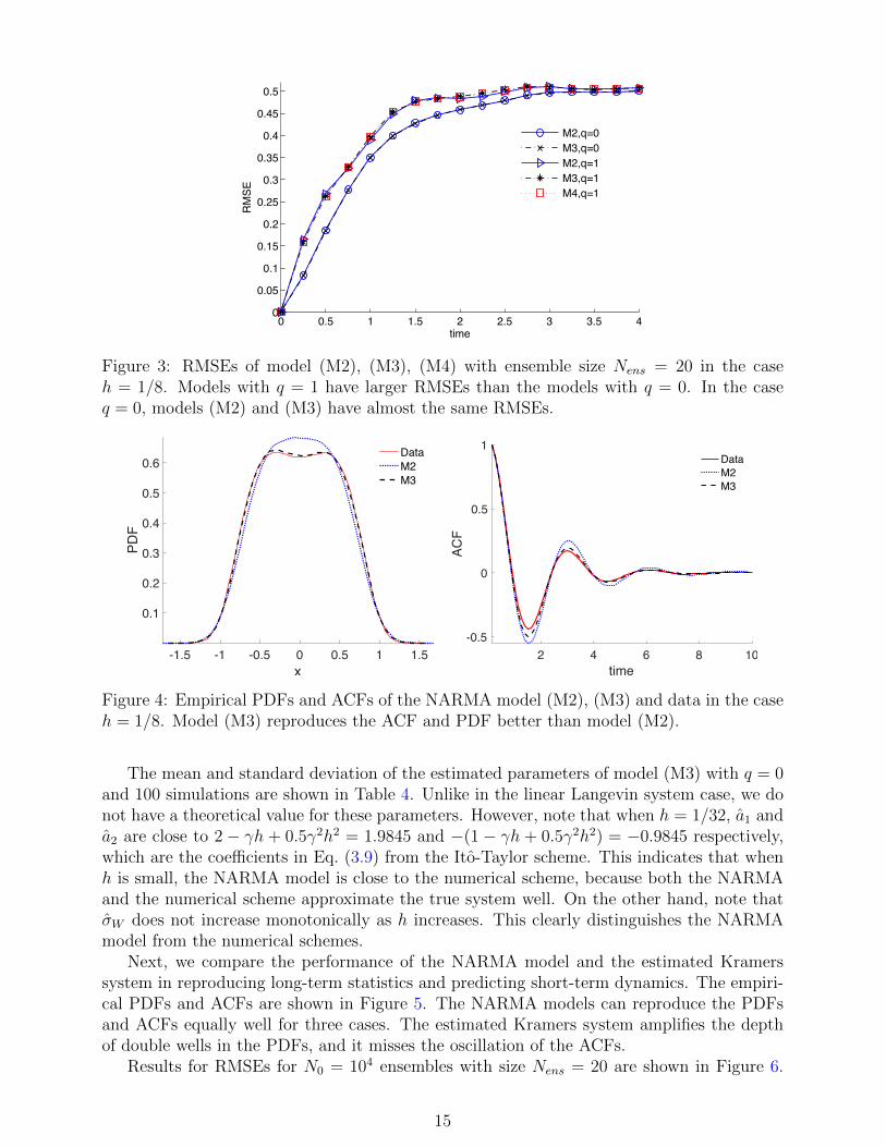
For the discrete-time approach, we have to select one of the four NARMA(2, q) models,Model (M1)–(M4). We make the selection using data only from a single long trajectory (e.g.from the time interval [0, T ] with T = 218 ≈ 2 × 105), and we use the first half of the datato estimate the parameters. We first estimate the parameters for each NARMA model withq = 0 and q = 1, using the conditional likelihood method described in Section 3.1. Then wemake a selection by the criteria proposed in Section 3.1. First, we test numerical stabilityby running the model for a large time for different realizations of the noise sequence. Wefind that for our model, using the values of h tested here, Model (M1) is often numericallyunstable, so we do not compare it to the other schemes here. (In situations where the Eulerscheme is more stable, e.g., for smaller values of h or for other models, we would expect it tobe useful as the basis of a NARMA approximation.) Next, we test the performance of eachof the models (M2)–(M4). The RMSEs of models (M2), (M3) with q = 0 and q = 1 andModel (M4) with q = 1 are shown in Figure 3. In the case q = 1, the RMSEs for models(M2)–(M4) are very close, but they are larger than the RMSEs of models (M2) and (M3)with q = 0. To make further selection between models (M2) and (M3) with q = 0, we testtheir reproduction of the long-term statistics. Figure 4 shows that model (M3) reproducesthe ACFs and PDFs better than model (M2), hence model (M3) with q = 0 is selected.

14

0 0.5 1 1.5 2 2.5 3 3.5 40

0.05

0.1

0.15

0.2

0.25

0.3

0.35

0.4

0.45

0.5

time

RM

SE

M2,q=0M3,q=0M2,q=1M3,q=1M4,q=1

Figure 3: RMSEs of model (M2), (M3), (M4) with ensemble size Nens = 20 in the caseh = 1/8. Models with q = 1 have larger RMSEs than the models with q = 0. In the caseq = 0, models (M2) and (M3) have almost the same RMSEs.

-1.5 -1 -0.5 0 0.5 1 1.5x

0.1

0.2

0.3

0.4

0.5

0.6

PDF

DataM2M3

2 4 6 8 10time

-0.5

0

0.5

1AC

FDataM2M3

Figure 4: Empirical PDFs and ACFs of the NARMA model (M2), (M3) and data in the caseh = 1/8. Model (M3) reproduces the ACF and PDF better than model (M2).

The mean and standard deviation of the estimated parameters of model (M3) with q = 0and 100 simulations are shown in Table 4. Unlike in the linear Langevin system case, we donot have a theoretical value for these parameters. However, note that when h = 1/32, a1 anda2 are close to 2 − γh + 0.5γ2h2 = 1.9845 and −(1 − γh + 0.5γ2h2) = −0.9845 respectively,which are the coefficients in Eq. (3.9) from the Ito-Taylor scheme. This indicates that whenh is small, the NARMA model is close to the numerical scheme, because both the NARMAand the numerical scheme approximate the true system well. On the other hand, note thatσW does not increase monotonically as h increases. This clearly distinguishes the NARMAmodel from the numerical schemes.

Next, we compare the performance of the NARMA model and the estimated Kramerssystem in reproducing long-term statistics and predicting short-term dynamics. The empiri-cal PDFs and ACFs are shown in Figure 5. The NARMA models can reproduce the PDFsand ACFs equally well for three cases. The estimated Kramers system amplifies the depthof double wells in the PDFs, and it misses the oscillation of the ACFs.

Results for RMSEs for N0 = 104 ensembles with size Nens = 20 are shown in Figure 6.

15

Table 4: Mean and standard deviation of the estimators of the parameters of the NARMAmodel (M3) with q = 0 in the discrete-time approach, computed from 100 simulations.

Estimator h = 1/32 h = 1/16 h = 1/8a1 1.9906 (0.0004) 1.9829 (0.0007) 1.9696 (0.0014)−a2 0.9896(0.0004) 0.9792 (0.0007) 0.9562 (0.0014)

−b1 0.3388 (0.1572) 0.6927 (0.0785) 1.2988 (0.0389)

b2 0.0300 (0.1572) 0.0864 (0.0785) 0.1462 (0.0386)

b3 0.0307 (0.1569) 0.0887 (0.0777) 0.1655 (0.0372)−µ (×10−5) 0.0377 (0.0000) 0.1478 (0.0000) 0.5469 (0.0001)

σW 0.0045 (0.0000) 0.1119 (0.0001) 0.0012 (0.0000)

-1 0 1x

0

0.1

0.2

0.3

0.4

0.5

0.6

0.7

PDF

DataNARMAEst. SDE

-1 0 1x

DataNARMAEst. SDE

-1 0 1x

DataNARMAEst. SDE

0 5 10time

-0.5

0

0.5

1

ACF

DataNARMAEst. SDE

0 5 10time

DataNARMAEst. SDE

0 5 10time

DataNARMAEst. SDE

Figure 5: Empirical PDFs and ACFs of the NARMA model (M3) with q = 0 and theestimated Kramers system, in the cases h = 1/32 (left column), h = 1/16 (middle column)and h = 1/8 (right column). These statistics are better reproduced by the NARMA modelsthan by the estimated Kramers systems.

16

0 1 2 3 40

0.1

0.2

0.3

0.4

0.5

0.6

time

RM

SE

True SDENARMAEst. SDE

0 1 2 3 4time

True SDENARMAEst. SDE

0 1 2 3 4time

True SDENARMAEst. SDE

h=1/32 h=1/16 h=1/8

Figure 6: The Kramers system: RMSEs of 104 forecasting ensembles with size Nens = 20,produced by the true Kramers system, the Kramers system with estimated parameters, andthe NARMA model (M3) with q = 0. The NARMA model has almost the same RMSEsas the true system for all the observation spacings, while the estimated system has largerRMSEs.

Table 5: Consistency test. Values of the estimators in the NARMA models (M2) and (M3)with q = 0. The data come from a long trajectory with observation spacing h = 1/32. HereN = 222 ≈ 4× 106. As the length of data increases, the estimators of model (M2) have muchsmaller oscillation than the estimators of model (M3).

Data length Model (M2) Model (M3)

(×N) −b1 −b2 −b1 b2 b3

1/8 0.3090 0.3032 0.3622 0.0532 0.05631/4 0.3082 0.3049 0.3290 0.0208 0.02171/2 0.3088 0.3083 0.3956 0.0868 0.08451 0.3087 0.3054 0.3778 0.0691 0.0697

The NARMA model reproduces almost exactly the RMSEs of the true Kramers system forall three step-sizes, while the estimated Kramers system has increasing error as h increases,due to the increasing biases in the estimators.

Finally, in Figure 7, we show some results using a much smaller observation spacing,h = 1/1024. Figure 7(a) shows the estimated parameters, for both the continuous anddiscrete-time models. (Here, the discrete-time model is M2.) Consistent with the theoryin [30], our parameter estimates for the continuous time model are close to their true valuesfor this small value of h. Figure 7(b) compares the RMSE of the continuous-time anddiscrete-time models on the same forecasting task as before. The continuous-time approachnow performs much better, essentially as well as the true model. Even in this regime, however,the discrete-time approach remains competitive.

4.3 Criteria for structure design

In the above structure selection between model (M2) and (M3), we followed the criterion ofselecting the one that fits the long-term statistics best. However, there is another practicalcriterion, namely whether the estimators converge as the number of samples increases. Thisis important because the estimators should converge to the true values of the parameters ifthe model is correct, due to the consistency discussed in Section 3.1. Convergence can be

17

Continuous-time model parameters

γ −β σ0.5163 0.3435 1.0006

Discrete-time model parameters

a1 −a2 −b1

1.9997 0.9997 0.0097

−b2 −µ(×10−8) σW (×10−10)0.0169 2.0388 6.2165 0 0.5 1 1.5 2 2.5 3 3.5

0.1

0.2

0.3

0.4

0.5

time

RM

SE

True SDENARMAEst. SDE

(a) Estimated parameter values (b) h = 1/1024

Figure 7: (a) Estimated parameters for the continuous-time and discrete-time models. (b)RMSEs of 103 forecasting ensembles with size Nens = 20, produced by the true Kramerssystem (True SDE), the Kramers system with estimated parameters(Est. SDE), and theNARMA model (M2) with q = 0. Since h = 1/1024 is relatively small, the NARMA modeland the estimated system have almost the same RMSEs as the true system. Here the datais generated by the Ito-Taylor solver with step size dt = 2−15 ≈ 3× 10−5, and data length isN = 222 ≈ 4× 106.

tested by checking the oscillations of estimators as data length increases: if the oscillationsare large, the estimators are likely not to converge, at least not quickly. Table 5 shows theestimators of the coefficients of the nonlinear terms in model (M2) and (M3), for differentlengths of data. The estimators b1, b2 and b3 of model (M3) are unlikely to be convergent,since they vary a lot for long data sets. On the contrary, the estimators b1 and b2 of model(M2) have much smaller oscillations, and hence they are likely to be convergent.

These convergence tests agree with the statistics of the estimators on 100 simulations inTables 4 and 6. Table 4 shows that the standard deviations of the estimators b1, b2 and b3 ofmodel (M3) are reduced by half as h doubles, which is the opposite of what is supposed tohappen for an accurate model. On the contrary, Table 6 shows that the standard deviationsof the parameters of model (M2) increase as h doubles, as is supposed to happen for anaccurate model.

In short, model (M3) reproduces better long-term statistics than model (M2), but theestimators of model (M2) are statistically better (e.g. in rate of convergence) than theestimators of model (M3). However, the two have almost the same prediction skill as shownin Figure 3, and both are much better than the continuous-time approach. It is unclearwhich model approximates the true process better, and it is likely that neither of them isoptimal. Also, it is unclear which criterion is better for structure selection: fitting the long-term statistics or consistency of estimators. We leave these issues to be addressed in futurework.

18

Table 6: Mean and standard deviation of the estimators of the parameters(a1, a2, b1, b2, µ, σW ) of the NARMA model (M2) with q = 0 in the discrete-time approach,computed on 100 simulations.

Estimator h = 1/32 h = 1/16 h = 1/8a1 1.9905 (0.0003) 1.9820 (0.0007) 1.9567 (0.0013)−a2 0.9896 (0.0003) 0.9788 (0.0007) 0.9508 (0.0014)

−b1 0.3088 (0.0021) 0.6058 (0.0040) 1.1362 (0.0079)

−b2 0.3067 (0.0134) 0.5847 (0.0139) 0.9884 (0.0144)−µ (×10−5) 0.0340 (0.0000) 0.1193 (0.0000) 0.2620 (0.0001)

σW 0.0045 (0.0000) 0.1119 (0.0001) 0.0012 (0.0000)

5 Concluding discussion

We have compared a discrete-time approach and a continuous-time approach to the data-based stochastic parametrization of a dynamical system, in a situation where the data areknown to have been generated by hypoelliptic stochastic system of a given form. In thecontinuous time case, we first estimated the coefficients in the given equations using thedata, and then solved the resulting differential equations; in the discrete-time model, wechose structures with terms suggested by numerical algorithms for solving the equations ofthe given form, with coefficients estimated using the data.

As discussed in our earlier papers [8, 21], the discrete-time approach has several a prioriadvantages:

(i) the inverse problem of estimating the parameters in a model from discrete data is ingeneral better-posed in a discrete-time than in a continuous-time model. In particular,the discrete time representation is more tolerant of relatively large observation spacings.

(ii) once the discrete-time parametrization has been derived, it can be used directly innumerical computation, there is no need of further approximation. This is not a majorissue in the present paper where the equations are relatively simple, but we expect itto grow in significance as the size of problems increases.

Our example validates the first of these points; the discrete-time approximations generallyhave better prediction skills than the continuous-time parametrization, especially when theobservation spacing is relatively large. This was also the main source of error in the continuousmodels discussed in [8]; note that the method for parameter estimation in that earlier paperwas completely different. Our discrete-time models also have better numerical properties,e.g., when all else is equal, they are more stable and produce more accurate long termstatistics than their continuous-time counterparts.

We expect the advantages of the discrete-time approach to become more marked as oneproceeds to analyze systems of growing complexity, particularly larger, more chaotic dynam-ical systems. A number of questions remain, first and foremost being the identification ofeffective structures; this is of course a special case of the difficulty in identifying effectivebases in the statistical modeling of complex phenomena. In the present paper we introducedthe idea of using terms derived from numerical approximations; different ideas were intro-duced in our earlier work [21]. More work is needed to generate general tools for structuredetermination.

Another challenge is that, even when one has derived a small number of potential struc-tures, we currently do not have a systematic way to identify the most effective model. Thus,

19

the selection of a suitable discrete-time model can be labor-intensive, especially comparedto the continuous-time approach in situations where a parametric family containing the truemodel (or a good approximation thereof) is known. On the other hand, continuous-timeapproaches, in situations where no good family of models is known, would face similar diffi-culties.

Finally, another open question is whether discrete-time approaches generally producemore accurate predictions than continuous-time approaches for strongly chaotic systems.Previous work has suggested that the answer may be yes. We plan to address this questionmore systematically in future work.

Acknowledgments. We would like to thank the anonymous referee and Dr. Robert Sayefor helpful suggestions. KKL is supported in part by the National Science Foundation undergrant DMS-1418775. AJC and FL are supported in part by the Director, Office of Science,Computational and Technology Research, U.S. Department of Energy, under Contract No.DE-AC02-05CH11231, and by the National Science Foundation under grant DMS-1419044.

A Solutions to the linear Langevin equation

Denoting

Xt=

(xtyt

),A =

(0 1−α−γ

), e =

(0σ

),

we can write Eq. (3.4) asdXt= AXtdt+ edBt.

Its solution is

Xt = eAtX0 +

∫ t

0

eA(t−u)edBu.

The solution at discrete times can be written as

x(n+1)h = a11xnh + a12ynh +Wn+1,1,

y(n+1)h = a21xnh + a22ynh +Wn+1,2,

where aij =(eAh)ij

for i, j = 1, 2, and

Wn+1,i = σ

∫ h

0

ai2(u)dB (nh+ u) (A.1)

with ai2(u) =(eA(h−u)

)i2

for i = 1, 2. Note that if a12 6= 0, then from the first equation

we get ynh =(x(n+1)h − a11xnh − Vn+1,1

)/a12. Substituting it into the second equation we

obtain

x(n+2)h = (a11 + a22)x(n+1)h + (a12a21 − a11a22)xnh

−a22Wn+1,1 + a12Wn+1,2 +Wn+2,1.

Combining with the fact that a11 + a22 = trace(eAh) and a12a21 − a11a22 = −e−γh, we have

x(n+2)h = trace(eAh)x(n+1)h − e−γhxnh − a22Wn+1,1 +Wn+2,1 + a12Wn+1,2. (A.2)

Clearly, the process {xnh} is a centered Gaussian process, and its distribution is de-termined by its autocovariance function. Conditionally on X0, the distribution of Xt isN (eAtX0,Σ(t)), where Σ(t) :=

∫ t0eAueeT eATudu. Since α, γ > 0, the real parts of the

20

eigenvalues of the A, denoted by λ1 and λ2, are negative. The stationary distribution isN (0,Σ(∞)), where Σ(∞) = limt→∞Σ(t). If X0 has distribution N (0,Σ(∞)), then the pro-cess (Xt) is stationary, and so is the observed process {xnh}. The following lemma computesthe autocorrelation function of the stationary process {xnh}.

Lemma A.1 Assume that the system (3.4) is stationary. Denote by {γj}∞j=1 the autoco-variance function of the stationary process {xnh}, i.e. γj := E[xkhx(k+j)h] for j ≥ 0. Then

γ0 = σ2

2αγ, and γj can be represented as

γj = γ0 ×{

1λ1−λ2 (λ1e

λ2jh − λ2eλ1jh), if γ2 − 4α 6= 0;

eλ0jh(1− λ0jh), if γ2 − 4α = 0

for all j ≥ 0, where λ1 and λ2 are the different solutions to λ2 +γλ+α = 0 when γ2−4α 6= 0,and λ0 = −γ/2.

Proof. Let Γ(j) := E[XkhXT(k+j)h] = Σ(∞)eAT jh for j ≥ 0. Note that γj = Γ11(j), i.e., γj is

the first element of the matrix Γ(j). Then it follows that

γ0 = Σ11(∞), γj =(Σ(∞)eAT jh

)11.

If γ2 − 4α 6= 0, then A has two different eigenvalues λ1 and λ2, and it can be written as

A = QΛQ−1 with Q =

(1 1λ1 λ2

),Λ =

(λ1 00 λ2

).

The covariance matrix Σ(∞) can be computed as

Σ(∞) = limt→∞

∫ t

0

QeΛuQ−1eeTQ−T eΛTuQTdu = σ2

(1

2ab0

0 − 12b

). (A.3)

This gives γ0 = Σ11(∞) = σ2

2γαand for j > 0,

γj = Σ11(∞)(eAT jh

)11

=1

λ1 − λ2

(λ1eλ2jh − λ2e

λ1jh)γ(0).

In the case γ2 − 4α = 0, A has a single eigenvalue λ0 = −γ2, and it can be transformed

to a Jordan block

A = QΛQ−1 with Q =

(1 0λ0 1

),Λ =

(λ0 10 λ0

).

This leads to the same Σ(∞) as in (A.3). Similarly, we have γ0 = σ2

2γαand

γj = Σ11(∞)(eAT jh

)11

= eλ0jh(1− λ0jh)γ0.

21

B ARMA processes

We review the definition and computation of autocovariance function of ARMA processes inthis subsection. For more details, we refer to [4, Section 3.3].

Definition B.1 The process {Xn, n ∈ Z} is said to be an ARMA(p, q) process if it is sta-tionary process satisfying

Xn − φ1Xn−1 − · · · − φpXn−p = Wn + θ1Wn−1 + · · ·+ θqWn−q, (B.1)

for every n, where {Wn} are i.i.d N (0, σ2W ), and if the polynomials φ(z) := 1−φ1z−· · ·−φpzp

and θ(z) := 1 + θ1z + · · · + θqzq have no common factors. If {Xn − µ} is an ARMA(p, q)

process, then {Xn} is said to be an ARMA(p, q) process with mean µ. The process is causalif φ(z) 6= 0 for all |z| ≤ 1. The process is invertible if θ(z) 6= 0 for all |z| ≤ 1.

The autocovariance function {γ(k)}∞k=1 of an ARMA(p, q) can be computed from thefollowing difference equations, which are obtained by multiplying each side of (B.1) by Xn−kand taking expectations,

γ(k)− φ1γ(k − 1)− · · · − φpγ(k − p) =σ2W

∑k≤j≤q

θjψj−k, 0 ≤ k < max{p, q + 1}, (B.2)

γ(k)− φ1γ(k − 1)− · · · − φpγ(k − p) = 0, k ≥ max{p, q + 1}, (B.3)

where ψj in (B.2) is computed as follows (letting θ0 := 1 and θj = 0 if j > q)

ψj =

{θj +

∑0<k≤j φkψj−k, for j < max{p, q + 1};∑

0<k≤p φkψj−k, for j ≥ max{p, q + 1}.Denote (ζi, i = 1, . . . , k) the distinct zeros of φ(z) := 1− φ1z − · · · − φpzp, and let ri be the

multiplicity of ζi (hence∑k

i=1 ri = p). The general solution of the difference Eq. (B.3) is

γ(n) =k∑i=1

ri−1∑j=0

βijnjζ−ni , for n ≥ max{p, q + 1} − p, (B.4)

where the p constants βij (and hence the values of γ(j) for 0 ≤ j < max{p, q + 1} − p ) aredetermined from (B.2).

Example B.2 (ARMA(2, 0)) . For an ARMA(2,0) process Xn−φ1Xn−1−φ2Xn−2 = Wn,its autocovariance function is

γ(n) =

{β1ζ

−n1 + β2ζ

−n2 , if φ2

1 + 4φ2 6= 0;(β1 + β2n) ζ−n, if φ2

1 + 4φ2 = 0

for n ≥ 0, where ζ1, ζ2 or ζ are the zeros of φ(z) = 1− φ1z − φ2z2. The constants β1 and β2

are computed from the equations

γ(0)− φ1γ(1)− φ2γ(2) =σ2W ,

γ(1)− φ1γ(0)− φ2γ(1) = 0.

Example B.3 (ARMA(2, 1)) . For an ARMA(2,1) process Xn − φ1Xn−1 − φ2Xn−2 =Wn + θ1Wn−1, we have ψ0 = 1, ψ1 = φ1. Its autocovariance function is of the same form asthat in (B.2), where the constants β1 and β2 are computed from the equations

γ(0)− φ1γ(1)− φ2γ(2) =σ2W (1 + θ2

1 + θ1φ1),

γ(1)− φ1γ(0)− φ2γ(1) =σ2W θ1.

22

C Numerical schemes for hypoelliptic SDEs with additive noise

Here we briefly review the two numerical schemes, the Euler-Maruyama scheme and theIto-Taylor scheme of strong order 2.0, for hypoelliptic systems with additive noise

dx= ydt,

dy= a(x, y)dt+ σdBt,

where a : R2 → R satisfies suitable conditions so that the system is ergodic.In the following, the step size of all schemes is h, andWn = σ

√hξn, Zn = σh3/2

(ξn + ηn/

√3),

where {ξn} and {ηn} are two i.i.d sequences of N (0, 1) random variables.Euler-Maruyama (EM):

xn+1 =xn + ynh, (C.1)

yn+1 = yn + ha(xn, yn) +Wn+1.

Ito-Taylor scheme of strong order 2.0 (IT2):

xn+1 =xn + hyn + 0.5h2a (xn, yn) + Zn+1,

yn+1 = yn + ha (xn, yn) + 0.5h2[ax(xn, yn)yn +

(aay + 0.5σ2ayy

)(xn, yn)

](C.2)

+Wn+1 + ay(xn, yn)Zn+1 + ayy(xn, yn)σ2h

6(W 2

n+1 − h).

The Ito-Taylor scheme of order 2.0 can be derived as follows (see e.g. Kloeden andPlaten [14,18] ). The differential equation can be rewritten in the integral form:

xt =xt0 +

∫ t

t0

ysds,

yt = yt0 +

∫ t

t0

a(xs, ys)ds+ σ (Bt −Bt0) .

We start from the Ito-Taylor expansion of x :

xtn+1 =xtn + hytn +

∫ tn+1

tn

∫ t

tn

a(xs, ys)dsdt+ σIn+110

=xtn + hytn + 0.5h2a(xtn , ytn) + σIn+110 +O(h5/2),

where In+110 :=

∫ tn+1

tn(Bt −Btn) dt. To get higher order scheme for y, we apply Ito’s chain

rule to a(xt, yt):

a (xt, yt) = a (xs, ys) +

∫ t

s

[ax(xr, yr)yr + (aay + 0.5σ2ayy)(xr, yr)]dr + σ

∫ t

s

ay (xr, yr) dBr.

This leads to Ito-Taylor expansion for y (up to the order 2.0):

ytn+1 = ytn +

∫ tn+1

tn

a(xs, ys)ds+ σ(Btn+1 −Btn

)= ytn + ha (xtn , ytn) + σ

(Btn+1 −Btn

)+ ay(xtn , ytn)σIn+1

10 + ayy(xtn , ytn)σ2In+1110

+0.5h2[ax(xtn , ytn)ytn + (aay + 0.5σ2ayy)(xtn , ytn)] +O(h5/2

),

where In+1110 =

∫ tn+1

tn

∫ ttn

(Bs −Btn) dBsdt. Representing σ(Btn+1 −Btn

), σIn+1

10 and In+1110 by

Wn+1, Zn+1 and h6(W 2

n+1 − h) respectively, we obtain the scheme (C.2).

23

References

[1] E. B. Andersen. Asymptotic properties of conditional maximum-likelihood estimators.J. R. Stat. Soc. Series B, pages 283–301, 1970.

[2] D. F. Anderson and J. C. Mattingly. A weak trapezoidal method for a class of stochasticdifferential equations. Commun. Math. Sci., 9(1), 2011.

[3] L. Arnold and P. Imkeller. The Kramers oscillator revisited. In J. Freund and T. Poschel,editors, Stochastic Processes in Physics, Chemistry, and Biology, volume 557 of LectureNotes in Physics, page 280. Springer, Berlin, 2000.

[4] P. Brockwell and R. Davis. Time series: theory and methods. Springer, New York, 2ndedition, 1991.

[5] P. J. Brockwell. Continuous-time ARMA processes. Handbook of Statistics, 19:249–276,2001.

[6] P. J. Brockwell. Recent results in the theory and applications of CARMA processes.Ann. Inst. Stat. Math., 66(4):647–685, 2014.

[7] P. J. Brockwell, R. Davis, and Y. Yang. Continuous-time Gaussian autoregression.Statistica Sinica, 17(1):63, 2007.

[8] A. J. Chorin and F. Lu. Discrete approach to stochastic parametrization and dimensionreduction in nonlinear dynamics. Proc. Natl. Acad. Sci. USA, 112(32):9804–9809, 2015.

[9] S. Ditlevsen and M. Sørensen. Inference for observations of integrated diffusion processes.Scand. J. Statist., 31(3):417–429, 2004.

[10] D. Frenkel and B. Smit. Understanding molecular simulation: from algorithms to appli-cations, volume 1. Academic press, 2001.

[11] A. Gloter. Parameter estimation for a discretely observed integrated diffusion process.Scand. J. Statist., 33(1):83–104, 2006.

[12] G. A. Gottwald, D. Crommelin, and C. Franzke. Stochastic climate theory. In Nonlinearand Stochastic Climate Dynamics. Cambridge University Press, 2015.

[13] J. D. Hamilton. Time Series Analysis. Princeton University Press, Princeton, NJ, 1994.[14] Y. Hu. Strong and weak order of time discretization schemes of stochastic differential

equations. In Seminaire de Probabilites XXX, pages 218–227. Springer, 1996.[15] G. Hummer. Position-dependent diffusion coefficients and free energies from Bayesian

analysis of equilibrium and replica molecular dynamics simulations. New J. Phys.,7(1):34, 2005.

[16] A. C. Jensen. Statistical Inference for Partially Observed Diffusion Processes. PhD the-sis, University of Copenhagen, Faculty of Science, Department of Mathematical Sciences,2014.

[17] R. H. Jones. Jones fitting a continuous time autoregressive to discrete data. In D. F.Findley, editor, Applied Time Series Analysis II, pages 651–682. Academic Press, NewYork, 1981.

[18] P. E. Kloeden and E. Platen. Numerical Solution of Stochastic Differential Equations.Springer, Berlin, 3rd edition, 1999.

[19] D. Kondrashov, M. D. Chekroun, and M. Ghil. Data-driven non-Markovian closuremodels. Physica D, 297:33–55, 2015.

[20] H. A. Kramers. Brownian motion in a field of force and the diffusion model of chemicalreactions. Physica, 7(4):284–304, 1940.

[21] F. Lu, K. K. Lin, and A. J. Chorin. Data-based stochastic model reduction for theKuramoto–Sivashinsky equation. arXiv:1509.09279, 2015.

[22] A. J. Majda and J. Harlim. Physics constrained nonlinear regression models for time

24

series. Nonlinearity, 26(1):201–217, 2013.[23] J. C. Mattingly, A. M. Stuart, and D. J. Higham. Ergodicity for SDEs and approxi-

mations: locally Lipschitz vector fields and degenerate noise. Stochastic Process. Appl.,101:185–232, 2002.

[24] J. C. Mattingly, A. M. Stuart, and M. V. Tretyakov. Convergence of numerical time-averaging and stationary measures via Poisson equations. SIAM J. Numer. Anal.,48(2):552–577, 2010.

[25] G. N. Milstein and M. V. Tretyakov. Computing ergodic limits for Langevin equations.Physica D: Nonlinear Phenomena, 229(1):81–95, 2007.

[26] D. Nualart. The Malliavin calculus and related topics. Springer-Verlag, 2nd edition,2006.

[27] A. W. Phillips. The estimation of parameters in systems of stochastic differential equa-tions. Biometrika, 46(1-2):67–76, 1959.

[28] Y. Pokern, A. M. Stuart, and P. Wiberg. Parameter estimation for partially observedhypoelliptic diffusions. J. Roy. Statis. Soc. B, 71(1):49–73, 2009.

[29] P. B.L.S. Rao. Statistical Inference for Diffusion Type Processes. Oxford UniversityPress, 1999.

[30] A. Samson and M. Thieullen. A contrast estimator for completely or partially observedhypoelliptic diffusion. Stochastic Process. Appl., 122(7):2521–2552, 2012.

[31] L. Schimansky-Geier and H. Herzel. Positive Lyapunov exponents in the Kramers oscil-lator. J. Stat. Phys., 70(1-2):141–147, 1993.

[32] H. Sørensen. Parametric inference for diffusion processes observed at discrete points intime: a survey. Int. Stat. Rev., 72(3):337–354, 2004.

[33] M. Sørensen. Estimating functions for diffusion-type processes. In M. Kessler, A. Lind-ner, and M. Sørensen, editors, Statistical Methods for Stochastic Differential Equations.Oxford University Press, London, 2012.

[34] D. Talay. Stochastic Hamiltonian systems: exponential convergence to the invariantmeasure, and discretization by the implicit Euler scheme. Markov Process. RelatedFields, 8(2):163 – 198, 2002.

25