TRANSPORTATION RESEARCH RECORD 1293 6t

Comparison of Computer Predictions and Field Data for Dynamic Analysis of Falling Weight Deflectometer Data

ALLEN H. MAGNUSON, ROBERT L. LYTTON, AND ROBERT C. BRIGGS

The extraction of e11ginee ring properties of pavemen t layers by dynamic analy ·is of falling weight deflectometer (PWD) dati1 is demon tratecl. FWD data fr m two in- ervicc highway ections were analyzed. The FWD data consist of time record of urface load.ing and surface deflections at a range of disiance . A Texas Transportation ]nstitu te pavement dynamics computer pr gram

ALPOT, wa used to generate predicred responses. Physical properties of the pavement were generated by n tria l-and-error backcalculation and a ysrcm Identification computer pro ram . The pavement surface vertiC<ll deflection were .charncterized by 11 ·ing frequency re. ponse functions in the form of magnitude and phase angle plot as a famction of frequency. 1l1e magnitude plot. represent vertical pavement surface deformation re ulting from a steady- tale inu oidal urface loadi ng. The pha e angle data repre enr the lag angle between the loading and the surface d -tlections. The asphallic concrete surrace layer wa represe nted as a three-parameter viscoelastk medium. The base cour e, subgrade layer ', and bedrock layers if any. were treated as d<imped ela tic olids. These phy ical pr pertie · were backcalculated by marching

approximately the frequency-analyzed field da ta with computed val ues by varying ihe CALP T input dar, set. Go d agreem nt between experimental and computer-predicted responses was b­rained using th ba kcalculated pavement lnyer pr pertic . One ite with near- urface bedrock was analyzed and good agreem nt

was obtained .

Dynamic analysis is governed by various forms of Newton's second law. In continuum mechanics Newton 's law is usually expre sed as the Navier vector field equati n. For an axisym­metric, horizontally laye red, viscoelastic medium (a highway pavement ection), th vector fie ld equation can be separated into two scala r reduced wave equations, each having its own calar potential. The equations can be solved readily by u ·ing

separation of variables and a suitable rth n rm al eigen­function cxpansi n. T he expanded lut ion can be evaluated numerically with specially formulated computer algorithms which may be implemented in one or more computer pro­grams. Thi proce s has been completed for the pavement dynamics problem , and some initial re ult a re presented.

Dynamic ana lysis require · unde r landing of ere p compli­ance function complex moduli, wave phen me na, dynamic vector fie ld equations compre ional wave , hear waves laye red media and many Olher physical phenomena , as well as variou applied mathematics disciplines and num rical methods. By contra t sta tic analysis i · u ua lly formulated

A. H. Magnuson and R. L. Lytton, Texas Transportation Institute, Texas A&M University System, College Station , Tex. 77843. R. C. Briggs, Texas State Department of Highways and Public Transpor· talion, Austin, Tex . 78701.

using the biharmonic operator, which is a special case (zero frequency) of the two reduced wave operators in the corre­sponding dynamic formulation.

NEED FOR PAVEMENT DYNAMIC ANALYSIS

One may well a k, Why u e dynamic analysis when tahc analy i me thods are readil available? Whal, if anything, is wrong wiih existing stntic analy ·i pr cedurcs? These ques­tions can be answered as follows:

• Dynamic analysis is more accurate and physically real­istic, becaus it takes into account transient (time-dependent) wave phenomena in the pavement layers .

• More inf rmation on pav men t layer properties can be extracted, because all the information in the falling weight deflectometer (FWD) time-pulse data is used in the backcal­culati n procedure (as oppo ed to only peak value f the pulses, a is current! done in e la. to-static analysis).

• Wit11 dynamic Malysis , the viscoela tic propertie. of chc asphaltic concre te (A ) ·urface layer can be characterized by creep c mpliance functi n in the time domain and complex moduli in the frequency domain. ta tic analy ·i · i limited to elastic modeling because viscoelastic phenomena are inher­ently dynamic.

•More phy ical insight into the pavement section ( .g. , lhe presence of bedrock , moda l respon e . . and reflection and refractio.n between layers) can be obtained from dynamic analysis.

• Dynamic analy ·is is more . ensitive to pavement laye r properties because of the additi nal data available. Thi · means tha t , in principle, more accurate backcalculation re:-ult can be obtained.

Dynam ic a naly i. I o r ntially offers the following benefit : cost avings, fa t response time , and additional ngineering infonnation. Among the inh rent advantage of FWD dy­namic analysis are nondestructive testing of the pavement surface and inexp nsive, fast automated data acqui ·ilion and analysis .

BACKGROUND

In September 1987 the Materials , Pavements and Construc­tion Division of Texas Transportation Institute (TII) started

62

work on a 4-year research project, " Dynamic Analysis of Falling-Weight Deflectometer Data." The project is admin­istered by the Texas State Department of Highways and Public Transportation as part of FHWA's Cooperative Research Program. The project's purpose is to develop a computer model of pavement dynamic response and to apply it in the prediction and evaluation of pavement performance.

The division is using mechanistic approaches to characterize pavement failu1e aIHJ aging associated with cracking and rut­ting. The dynamic analysis of FWD data can, in principle, be used to backcalculate pavement layer properties related to remaining pavement life.

FWD (or drop weight force impulse) devices are in wide­spread use for in-service pavement evaluation and backcal­culation of moduli. However, pavement response data are currently analyzed with static models.

In static analysis the dynamic <leflection basin caused by the FWD is assumed to be static, whereby the instantaneous pavement deflection at a given point is assumed to be pro­portional to the instantaneous force on the pavement surface. In static analysis, therefore , only the peak values of the force and deflection pulses are used.

The FWD time-pulse data contain much more information on the pavement layers; however , this information cannot be extracted without a working pavement dynamic analysis pro­gram. Static analysis methods are used because no one has yet developed a practical working dynamic analysis program for pavements.

RELATED WORK

Pavement impulse testing is described by Lytton et al. (1) and Uzan et al. (2). Dynamic response of geophysical and geo­technical systems started with the work of Lamb (J) , who solved the problem of the dynamic response of a uniform half­space to describe the main features of earthquake tremors. Ewing et al. ( 4) is a standard reference in seismology for dynamic analysis of multilaye1eu elastic media. The analysis used in TTI's SCALPOT computer program is a direct ex­tension of this work.

Magnuson (5 ,6) developed a matrix recurrence relation to solve the multilayered viscoelastic problem for another ap­plication. The recurrence relation reduced the matrix rela­tions to a series of 4 x 4 matrix manipulations that could easily be programmed on a computer. He also introduced viscoelastic complex moduli into the multilayer problem by using the correspondence p1inciple. Each layer's response was characterized by two scalar potentials , one for the compres­sional wave and the other for the vertical shear wave. The solution is expressed as a Fourier-Bessel integral expansion. This expression is an improper integral having one or more pole singularities near the path of integration and an infinite upper limit. The integral is particularly difficult to evaluate accurately because of the slow convergence as the upper limit approaches infinity . Magnuson (7) describes an integration algorithm developed for the pavement dynamics problem. The algorithm is an extension of Zhongjin's analysis (8). The multilayered medium's matrix algebra (6) and the integration algorithm (7) have been incorporated into the SCALPOT computer program, which was developed for the dynamic analysis of pavement responses.

TRANSPORTATION RESEARCH RECORD 1293

SCALPOT AND FWD-FFT

The SCALPOT (scalar potential) program developed at TTI computes the dynamic response of a horizontally layered vis­coelastic half-space to a time-dependent surface pressure dis­tribution. Vertical surface deflections resulting from the os­cillatory surface pressure distribution can be obtained for a range of frequencies and distances from the surface pressure distribution .

SCALPOT has been modified to incorporate a surface layer. Additional modifications were made to treat pavement sec­tions with stiff layers and near-surface bedrock. The input data set for SCALPOT consists of the ge metrical configu­ration of the FWD apparatus and the physical properties of each pavement layer. The properties of each layer include thickness, weight density, viscoelastic parameters, Young's modulus, damping ratio, and Poisson 's ratio. SCALPOT is currently programmed to treat each layer as a damped elastic solid or as a three-parameter viscoelastic medium.

Another computer program developed at TTI, FWD-FFT, was used for analyzing the FWD data. The methods used to analyze the FWD data are described elsewhere (9). The pro­gram scans the time series data, makes the pulse " tail cor­rection ," computes averages, and performs a Fast Fourier Transform (FFT) of the corrected and averaged pulse data. FWD frequency response functions are then computed by performing a complex division of the FFT of the surface de­flections by the FFT of the surface loading. The frequency response functions are computed for the seven displacements at each site, and the results are written to data files and plotted.

FREQUENCY DOMAIN ANALYSIS

FWD time pulses are transformed to the frequency domain by using the superposition principle. The transient pulses are expressed as a sum of time-harmonic functions interfering with each other in such a way as to closely replicate the original pulse shape. This process is performed efficiently using FFTs, which are based on an algorithm formulated by Cooley and Tukey in the 1960s.

This study was conducted using frequency domain analysis, whereby the pavement surface vertical deflections were char­acterized with steady-state frequency response functions. At a given frequency, the vertical surface deflections are repres­ented as the response to a sinusoidal vertical surface loading. The data are presented in the form of magnitude and phase angle plots as a function of frequency. The phase angle repres­ents the lag angle (at a given frequency) between the loading and the surface deflections.

PAVE-SID

PAVE-SID, a computer program ba ed on the System IDen­tification (SID) methodology was developed to extra t pave­ment properties by using FWD data and dynamic analysi · techni.qu . PA VE-SlD is described by Torpunuri (10). The input to the program are the FWD experimental frequency response functions and computed responses generated by the

Magnuson et al.

ALPOT program. The SID method i · described in detail elsewher (U ,12). PAVE- ID uses S ALPOT t generate <L

data base for constructing a ensitivity matrix . lncrem 111 · in pavement layer propenie are computed from the field data and the ·cnsitivity matdx. The updated parameter are input into SCALPOT and the re. p nse is compu ted and compared against the field data. Tl) process is repeated until conver­gence is obtained.

PAVEMENT VISCOELASTIC PROPERTIES

An early study of viscoelastic properties of A materi.als wa conducted by Papazian (l 3). Papazian performed lab ratory creep tests on A core . am pies and used a lin ar Voigt-chain­Maxwell vise elastic representation (14) 10 m del the train data in both the time and frequency domain . Lai and An­der. on (15) used a nonlinear Voigt-chain-Maxwell viscoelastic representation to model Lhe creep and recovery of A material.

Paris' law gove rning crack propagation in a vi coelastic medium provides a direct link between pavement cracking and phy ical properties of the A material. chap ry (/6) put Paris' law on a sound mechanistic footing and developed a nonlinear fracture theory for viscoela, tic comp ite materials applicable to A pavement .

Pavement rutting re ulLing from permanent deformation f the A layer is characterized by Kenis's viscoelas tic system (YE YS) mu-alpha f rmulation (17). The VE YS f rmula­tion can be applied to the viscoelastic characleriw tion r th pavemenL to estimate remaining li fe before failure from rutting.

ANALYSIS OF FWD DATA

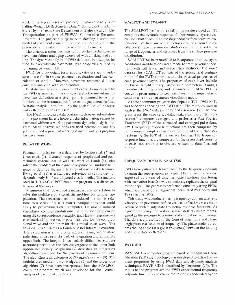
Figure 1 is a time plot of the FWD f rces and su rface de­flections for the District 1, Site 3 (DOl S3) pavemen t section

63

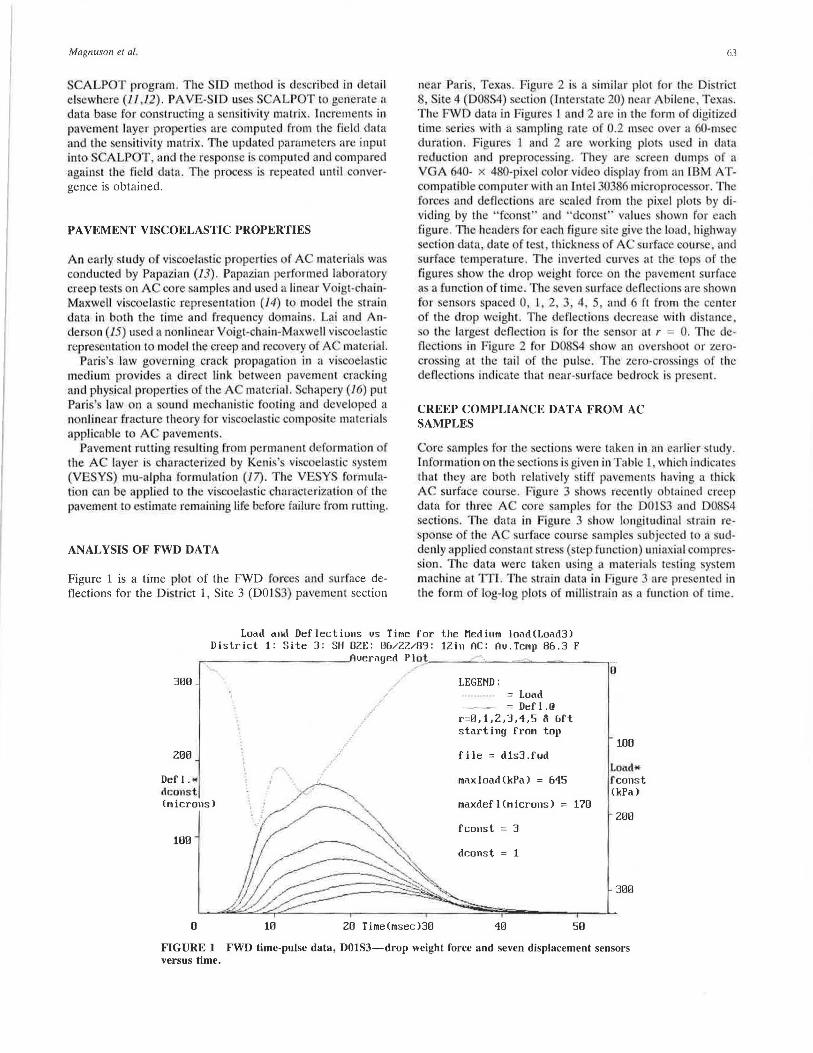
near Paris Texas. igure 2 is a similar pl t for the Di. trict 8 ite 4 (008 4) ection Interstat • 20) n ar Abil ne , Texas. The FWD data in Figures 1 and 2 ar in the form of digitized time series with a sampling rate of .2 msec over a 60-ms durnti n. Figure l and 2 are working plot · u cl in data reduction and preprocessing. They ar , creen dumps of a VGA 640- x 4 0-pixel color video di play from an IBM AT­c mpatible computer with an Inte l .10386 microproce ·s r. The forces and deflec1i n arc ·caled from the pixel plots by di­viding by the 'fcon t" and " dconst" values shown for each figure. The header· for each figure site give the load , highway ection data, date f tcsl , lhickness of A urface cours . and

surface temperature. The inverted curve · at the I. p ol' the figures show the drop weight force on the pavement urfac a a function of time. Th seven urface deflections are hown for sensors spaced 0, I , 2, 3, 4 5, an I 6 ft from the center of the drop weight. The dc(lections decrease with distance. o the largest deflection i: f r the sen or at r -= 0. The de­

flections in Figur 2 for DO S4 . how an ver ·ho L or z · ro­cro si ng at th tai l of the pulse. The zcro-cro sings of the deflections indicate that near-surface bedrock i. pr . ent.

CREEP COMPLIANCE DAT A FROM AC SAMPLES

Core samples for the section wer taken in an arlier s tud . Information on the sections is given in Table L which indicate, that they are both relatively tiff pavements ha ing a thick AC surface cour ·e. Figure 3 show recently obtained creep data for three A core sample. for the DO I 3 and 008. 4 section . The data in · igurc 3 show longi tudinal strain rc­·ponse of the A surface course amples ·ubjected to a ·ud­denJy applied con tant stre s ( tep function) uniaxial c mpre -·ion. The data were taken using a materials te. ting ystem machine at ITI. The strain data in Figure 3 arc presented in the form of log-log plot o f milli ·train as a function of time.

Load and Deflections vs Time for the Medium load(Load3) District 1: Site 3: SH 8ZE: 06/ZZ/89: 1Zin AC: Av.Temp 86 .3 F ~-----------'· veraged Plot,,__ ___ ~-~~-----..-

300

200

Def 1." dconst (microns)

100

0

,/

10 20 T ime(msec)30

LEGEND: = Load = Def!.@

r=0,1,2,3,1,5 a 6ft starting from top

file = d1s3. fwd

maxload(kPa) = 615

maxdefl(microns)

fconst = 3

dconst = 1

10

0

100

Load* fconst CkPa)

170 zoo

300

50

FIGURE 1 FWD time-pulse data, D01S3-drop weight force and seven displacement sensors versus time.

64 TRANSPORTA TION RESEARCH RECORD 1293

Load and Deflections us Time for the Medium load(Load3) District 8: Site 1: IH 20: 08/16/89: Win AC: Au.Temp 87 F

....----------~·ueraged P lo.t _ _ _ _ -..:.-~~-----.

300

200

Def I . " dcons t (microns)

100

0 10 20

LEGEND: = Load = Defl .@

r=0,1,2,3,1,5 a 6ft starting from top

file = d8s1 .fwd

maxload(kPa) = 517

maxdef I (microns) 181

fconst = 3

dconst = 1

so

0

um

Load* fconst CkPa)

200

300

FIGURE 2 FWD time-pulse data, D08S4-drop weight force and seven displacement sensors versus time.

TABLE 1 PAVEMENT SECTION CHARACTERISTICS (FROM CORE SAMPLING LOG)

Section Surface Course Base Course Subqrade

D01-S3 12 in thk AC 22

D08-S4 10 in thk AC 11

0 • • ! . 0 .......... : .. . ...... . . -:-··------··· : · .. .. ..... : ... . .. ..... :··~----

~ -- ; J / ~l~ ~ ~ ·····-~ r·;~" r:~ :;~ ' · 2 ,i;- ~ : ; + DD8S4- 1

N I

0

t . . x 00854-2 ······ ····-· .... .. .. ... .

10 - 2 10 -1 100 10 1 102 103 Time , s e c .

FlGUltE 3 Log-log 1>lot of millistrain from laboratory compressional creep le.st -one samplr. from DOIS3 and lwo sam11ll's from DOS '4.

PAVEMENT FREQUENCY RESPONSE FUNCTIONS

104

in

in

Figure 4 and 5 repre ent the frequency re ponse functions for pavement vertical surface defl ections resulting fr Ill a ver­tical ' urface pressur di. tri bution cau. eel by the · WD appa­ratu ·. or convenience, the magnitude re. p nscs are given in

(Sandy) Clay

LS CR Clay:Rock@ 9.75 ft

units of mil p r 10 kips in Figures 4a, 4c, 5a and Sc. Figure 4 how D01S3 fr quency re -ponse function. computed fr m FWD da ra using th FWD-FFr computer program. Data are hown or di placements a t r = 0, J. 2, 3 4, 5 and 6 ft .

Magnitude response· fo r rhe inner sen. or , phn e angles for rhe inner sensors, magnitude for the out r sen r. , and pha, e angle fo r the out r sensors arc hown in Figur s 4a 4b, 4c, ;md 4d resp ctively . T he magnitudes in Figures 4a and 4c decrease 1 ich r, o the r = 0 curve i on top , the r = 1 ft curve is immediately below it and o on. The phase angle cmves in Figure. 4b and 4d tart with the smalle. t r on top and work down as r increa. es. .

The e FWD frequency respome curve. b have the smn for all the sections examined so fa r· the general arrangem nt of the respon ·e curves in Figure 4 i the same for other sec­tions. The magnitude curv decrea e with frequency becau. e of the effect of the ma s through ewt n' law. imilarly the pba · angles increase with frequency.

The DOIS3 phase angle curves fo r r = 5 and 6 ft show a jump at the higher frequencies. The;: jump coincide · with a dip or parti al null in the rresponding magnitude curves. This beha ior indica t s wa e interference, or poss ibl modal re ·ponse caused by repeated back refl ection ff lower layers.

Figure 5 shows D08. 4 frequency rcspon e function com­put ct from FWD data using the FWD-FFT c mpu ter pro­gram. Data, whi h ar hown for the same displacement a f r · igure 4 are arranged in the ame way as the data in

001 , Site 3; r= 0, 1, 2 & 3 ft a:: 10 .----------------. :i 0 v ........ .!!! .E -Q.

"' 0

CIJ

°' c <

8

6

4

2

0 0 20 40 60 80 100 120 140

Frequency, Hz.

(a) Magnitudes, Inner Sensors

- 60 ''"'<:: : . :

·· ···: '""' ',':"""'-' ... .. . .. : ..... : ..... -: ; ' :' . ~ . :- ..+ - ;-: :'- '.\ • .. ;- . .. : .. . _:. .

· ··· · : ···••" · ·· ·~· ·"-- : ·····:···--; · ···· CIJ - 120 Ill 0 .t: ~

I O O - - o I

~ ~ ~ -=- - ~' . . . . -180,____.. _ _.__.....__~__.. _ _.___.. 0 20 40 60 80 100 120 140

Frequency , Hz.

(b) Phase Angles, Inner Sensors

001, Site 3; r= 4, 5 & 6 ft a:: 3 ..---- .----------.., :;;: - : 0 • )....

.::.. 2 . :: ,,; : -~- -~·-··· ···· ···- ·· · ··· .. ':;, - . ·. " E ... ) _: .. -:-: : :.~:·,',·: .. ··.~:;-- ···· ········· ··· . ; . ~ :· .. -.,.., : ~ ' : ;·t-... ·;. 0 0 ' I '

0 20 40 60 BO 100 120 140 Frequency, Hz.

(c) Magnitudes, Outer Sensors

Cl ., o, : : ·~ .... : .. .. "O

~ - 120 ····-~· ''\::~:·::.:. ("··~· .. ··( .. ~ : : ' : • .. .. ': . ......: ., - 240 .... . ~ ... .. ~ . ... ~ .. . . :. ?: ! '.'. : • ••. : .. . .. "' : . ; '-; ' .. : 0 . • • • •••

.r. : : ' :-~ - 360'----'"--'--~·-......... -~·-_._· ___,

0 20 40 60 BO 100 120 140 Frequency, Hz.

(d) Phase Angles, Outer Sensors

FIGURE 4 D01S3 frequency response functions (computed from FWD data) .

0 08 , Site 4; r= 0 , 1, 2 & 3 f t a:: 10 .-------- --- -----. :i 0 v ........ "' .E -Q.

"' 0

Cl CIJ

"O

CIJ

8

6

4

2

0 0

. . : . : : . .. .. ;. .. . ··\. · ....... .. ~ · ... . ; ..... ; .... . . ..... J,~ ; .i, .. : .. .. .. ~ . . ~ .... : ... .. ,,, . .., ~ -· . . .... . : .... --~- ~-;.~~ . ~ -~ ':'"~- -~ - ....

: : - : - :'~~·

20 40 60 BO 100 120 140 Frequency, Hz.

(a) Magnitudes, Inner Sensors

60..------- --- -------.

0. c ~ 60 ·····r ·--~~-.:~ ~--.t ·~ -~- -~: ;~ ---<

~ - 120 ·· · ··:-- - ······· · - ~ ·:,,,; ·~· :..: -,· ·· ... ··:, ···· 0 .t: ~

. . ..... ,, ., : : : ;.. ... . - 180 ,____.. _ _.__.....__~_.. _ _._~

0 20 40 60 80 100 120 140 Frequency, Hz.

(b) Phase Angles, Inner Sensors

008, Site 4; r= 4, 5 & 6 ft a:: 4,.-------------, :i S? 3 .. ... :.~ . .... ~ . .... : ..... : ..... : .. . . . ....., f · ·· \ : : : : ':;, 2 _ J.,~;. :. -~~ ... i. .... ; .... - ~ · .. ) ... .. .E ,.:f .\ ..... [ .. ~Y:-.\ .; .. ... t .. ) .... . ~ ··.::.:-.. ;:~. : .... 0 0 . . - . .

0 20 40 60 80 100 120 140 Frequency, Hz.

(c) Magnitudes, Outer Sensors

120 .-------------~

"' CIJ 'O

20 40 60 80 100 120 140 Frequency, Hz.

(d) Phase Angles, Outer Sensors

FIGURE S DOSS4 frequency response functions (computed from FWD data).

66

Figure 4. The magnitude <1nd pha. · angle curves differ con­siderably from the DOl S3 re pons s because of the near­surface bedrock. The magnitude response hav a pronounced peak at about 30 Hz. he peaking increase · f r increa ing distance r. There are two or three partial nulls in magnitude and corre ponding jumps in phas angle. In add ition the pha e angles of the inner enso rs how a cro sover a t about 2S Hz followed by a lead angle for lower frequencies. There i tip­

parently a nnection between the unu ua l behavior f the fr quency re ponse curves in the presence of bedr ck and th , time-pulse overshoot or zc~o -cros ing seen in Figure 2.

VISCOELASTIC REPRESENTATION OF AC MATERIAL

The simple t way to interpret the data in Figure 3 is to use a two-parameter power-law r presemaiion, as follows:

D(t) =At" (1)

wller /1 is the log-log slope and A is the intercept a t t = J sec. A three-parameter repre ·enrntion , n generalized time­domain power-law repre enta tion , i ' a l in ex te nsive u e. The ge ne ralized power-law or three-parameter repres "ntation eparatc. the viscoelastic pan fr m the (a ·umcd) e la tic re­p nse , and may be written as follow :

(2)

where D 0 is the elastic compliance and D 1 is the viscoelastic term evaluated at t = 1 sec.

Becau e f the reciprocal re lationship between compliances and mod uli , the first and second compliances in Equa tion 2 can b written a. fo llows:

(3a)

and

(3b)

wber £ 0 is the elastic modulus and £ 1 is the viscoelastic m du lus at t = 1 sec.

~ xpressing Equation 2 in terms of the moduli in Equation 3 give.

D(t) = 1/£0 + t"/E 1 (4)

This representation, when evaluated at t = 1 sec, is equivalent to two springs in series.

FREQUENCY DOMAIN REPRESENTATION OF AC CREEP COMPLIANCE

The time-domain creep compliance functions (Equations 1 and 2) must be transformed into the frequency domain for use in pavement dynamic analysis programs. The frequency­domain representation is called the complex compliance be­cause it can be expressed as a complex number having a real

TRANSPORTATION RESEARCH RECORD 1293

part and an imagi nary part. Performing a ·ourier imegral tra11sform on - quations l and 2 gives th following for the two- and three-parameter complex c mpliancc , respectively:

D(w) = Af(l + n)w-"[cos (mr/2) - isin (mr/2)] (5a)

D(w) = D 0 + D 1f(l + n)w-"[cos (mr/2)

- isin (mr/2)] (Sb)

where i = \/=T, w is the radian frequency, and r represents lhe gamma function.

Equation Sb, for the three-parameter representation, has been coded into the SCALP T pr gra m.

LABORATORY CREEP COMPLIANCE DATA

The D01S3 and DO S4 creep data in Figure 3 were u ed to obtain the viscoelastic parameters for the tbree-pararneter model hown in Equation 2. For th at representation th con­stant D 0 for the elastic component is an assumed value. The viscoelastic comp n nt wa obtai ned b subtracting o ut th a surned e la tic term fr m the l()tal creep data in Figure 3 and rcplotting the remaining train on a log-I g cale. T he vi coelastic parameter. 11 and 0 1 are o tain d from lh ·lope and int rcept, re peccively, of the log-log plots.

DESCRIPTION OF COMPARISON STUDY

The comparison study pre ented here wa onducted on cc­tion 00153 and 00854 because core sample. from the e ection w re left ver from a previous inve tigati n. The

sample were tested in uniaxia.I con · iant st rc s iu compre si n. This a llowed the invesiigators to ompnr backcalculated vis coelastic parameter brained from FWD data with laboratory te t re ult .

The frequency response functions . hown in · igure I and 2 w r c mparecl ~ ith corresponding compur I value gen­enned by th ALP program. The backcalculation study wa · performed by c ·ti mating lhe S A POT data set using creep data for A material and modulu dat ·1 gen rat d from tatic backcalculation efforts. The estimated data et was used

in the A P T program to obtain a first approximation t the surfac defl ·cti n . Followi 11 • the initial c tinrntes, the moduli, vi coela tic c n rnnts, and unknown layer thickness •s for ea h layer were ad ju t cl one at a lime on a trial-and-error ba. i until ·•n isfactory agreement with field data was achie ed.

Genern lly speaking. th re ponse. at th I \ frcquencie:. are d<>minated by the lowest layer. This ob. erva ti n led t th imroducti n f n.e\ ublayers by splining the subgrad or the bcd r ck , r both. int two. ublaycrs , with m du!tt in­creasing with depth. Thi subdivi ion improved the correla­tion at lo\ freq uencie · .

Section D01S3 was further subjected to an automated back­calcu lalion proced ure using the PA ~ - ID computer pr -gram . The fD study significantly impr ved agrcem~nt f the field data with compu l d re ' r onses. The SID stud' u. eel fre­quencic from <lpproxi mm ly I 0 to 130 Hz in I 0-Hz . icps.

Magnuson et al.

RESULTS OF COMPARISON STUDY

D01S3 Results

Figure 6 compares SCALPOT-computed values using the backcalculated three-parameter viscoelastic representation with frequency-analyzed FWD data. The symbols represent com­puted values and the solid line represents the FWD data. The FWD data are the same as in Figure 4. Figures 6a, 6b, 6c , and 6d show the magnitude response at r = 1 ft, the phase angle response at r = 1 ft, the magnitude response at r = 4 ft, and the phase angle response at r = 4 ft, respectively. There is good correlation of phase angle at both r = 1 ft and r = 4 ft. Magnitude correlation is good for r = 1 ft; however, some discrepancy is apparent at r = 4 ft. Nevertheless, the discrepancy is within 1 mil per 10 kips.

Figure 7 compares, for all displacement sensors at Section D01S3, the SCALPOT-computed values and the frequency­analyzed FWD data shown in Figure 4. It appears here to show the full data set used in the actual backcalculation pro­cess. The symbols represent computed values, and the solid lines represent the FWD data. Figures 7a and 7b show the magnitude and phase angle responses, respectively, at r = 0, 1, 2, and 3 ft; Figures 7c and 7d show the magnitude and phase angle responses, respectively , at r = 4, 5, and 6 ft. There is good agreement for both magnitude and phase angle at all values of r. At a given frequency the magnitudes are larger for smaller values of r, and the phase angles increase with r.

The agreement of the outer sensors in Figure 7c does not appear to be as good as the inner sensors' correlation . This

D01, Site 3; r = 1 ft a: 10..----------------. :;;:

s a ... ·- ....... . . ~·· ..•.... . .... •.... ...._.. 6 • . : . . '-. 6 . A. ·~ ..... .. ~ .... : .•• • : . • • ·~ •. ..

"' .E

a. .!!? 0 0 ..___.. _ _,__....._____..____.._ ........ __,

0

(a)

20 40 60 80 100 120 140

Frequency, Hz.

Magnitude, r = 1 ft Sensor

o.---------------. O'I Q)

-o -JO Q)

O'I c:: -60 <(

Q) (/) -90 Cl

..c:: ~ -120..___... _ _._ _ _,__.___.... _ _.___.

0 20 40 60 BO 100 120 140

Frequency, Hz.

(b) Phase Angle, r = 1 ft Sensor

67

is because the magnitudes are shown on an expanded scale. The absolute correlation for all the magnitudes is within 0.5 to 1 mil per 10 kips , which is the limit of resolution of the geophones. The good overall agreement can be attributed to the use of the PA VE-SID program in the backcalculation.

Table 2 shows pavement layer thicknesses, including the backcalculated thickness of the upper subgrade layer. Table 3 shows viscoelastic parameters £ 0 , £ 1, and n for the AC surface course; backcalculated values for Young's modulus; and damping for the base course and both subgrade layers. Table 4 compares viscoelastic parameters obtained from lab­oratory tests with those obtained from backcalculation.

D08S4 Results

Figures 8 and 9, respectively, show information for Section D08S4 corresponding to that shown in Figures 6 and 7 for Section D01S3. Again there is good agreement for both mag­nitude and phase angle for all values of r. Agreement at frequencies below approximately 10 Hz is poor, apparently because of the hyperbolic behavior of the complex modulus in Equation Sb. To avoid this, a four-parameter model for the AC surface course would be necessary.

From coring data, this section was known to have a near­surface bedrock layer at a depth of 9.75 ft (see Table 1). For this reason, the section was initially treated as a four-layered section, with a three-parameter viscoelastic AC layer, a base course, a subgrade layer, and the infinitely deep bedrock layer. In addition to the moduli of the top three layers, the depth to bedrock and the bedrock 's modulus were backcal-

D01, Site 3; r = 4 ft a: 4..----------------, :.;; . . . . ~ 3 ll" .. ~ •. • ·:· . - . ~ · - - • ~ - • - - : - .•. ~ ..• •

' .6 : • • ~ 2 · · ·· ~· · : . . 4 . ~····'. .... : .... ~ · · · · E

a. .!!?

: "' ~---..· ..;.· .:.:···""····

. " a o .__. _ __.__.....__..____.. _ _.____.

O'I Q) -0

o

(c)

Cl> -120

°' c:: <(

Q) -240 (/)

Cl ..c::

20 40 60 80 100 120 140

Frequency, Hz.

Magnitude, r = 4 ft Sensor

-· .. ;. --- .:. -- --:-.. -.-: ·-·· i- --- :· - ~-. . . . . . o • I t

" ' I '

~ -360'-----~-...._-~----~~ 0 20 40 60 BO 100 120 140

Frequency, Hz.

(d) Phase Angles, r = 4 ft Sensor

FIGURE 6 D01S3 frequency response functions for r = 1 ft and r = 4 ft: comparison between computed values (symbols) using backcalculated three-parameter viscoelastic representation and frequency-analyzed FWD data (li11es).

001, Site 3; r= 0, 1, 2 & 3 ft Cl:: 12.-~~~~~~~~~~~--. :.;<

10 ' 0 I 0

•••• :- . . • -:- • . • -: • - •• ~ .. . . . i • • - • :- - - •• . . . . . .

20 4-0 60 BO 100 120 1+0

Frequency, Hz.

(a) Magnitudes, Inner Sensors

-60

Ol c - 120

<{

ii) V> -160 0

.<:

.... ;: . , ~ .. ._ .~ . O-R .0 . 9 ... ~ . . ; ·: ... o-1 -.... : ~"' ~6 -~· o.

: : : :t::: I:: : f · Q '. r'. ~ T ;J~ :: : ~ -240L---'~-'-~-'-~ ....... ~.._~.____,

0 20 40 60 80 100 120 140

Frequency, Hz .

(b) Phase Angles, Inner Sensors

001, Site 3; r= 4, 5 & 6 ft a: 4.-~~~~~~~~~~~~ :.;<

C1 3 A·· -~ · • • .• . .. .. • ,: • · · · ; · · · ·: · · · · ~ • · · · ~ ~~ .. : : . :

~ 2 ;o:,~:'m~-~-~·-- - ~ - - -· ; ··· · ~ · -·· E ~ ~ ~ • .. ~-, ~~ i._ ~ i : : 0.. 1 ••• ·:· • . ·--;· ·' •• :.;~ ."''-V 'O:." . ~ ... . (/) : : ~ ~ ~:· ··.:-: <!~-· i5 0 -

Ol ii)

"O

0 20 +o 60 BO 100 120 140

Frequency, Hz.

(c) Magnitudes, Outer Sensors

ii) - 120

°' c <{

20 40 60 BO 100 120 140

Frequency, Hz.

(d) Phase Angles, Outer Sensors

FIGURE 7 DOIS3 frequency response functions for all displacement sensors: comparison between computed values (symbols) using backcalculated three-parameter viscoelastic representation and frequency-analyzed FWD data (lines).

TABLE 2 PAVEMENT LAYER THICKNESS (INCHES)

Site D01S3 DOBS4

Laver Thickness Deoth Thickness Death

AC Surf ace 12 12 10 10

Base 22 34 11 21

Subgrade 20* 54 72* 93

SG-2/BR-1 "' - 48* 141

Bedrock-2 - - "' -

* Back-Calculated Value

Note: SG indicates subgrade; BR indicates bedrock.

TABLE 3 BACKCALCULATED PAVEMENT LAYER MODULI AND DAMPING

Site D01S3 D08S4

Layer Modulus Damping Modulus Damping (KSil (KSI)

AC Surf. (3-Par) 0.296* 0.30*

EO 834.0 1250.0

El 1516.4 1250.0

E @ 10 msec 731 999.0

Base Course 45.11 0.015 104.2 0.015

Subgrade l 20 . 17 0.015 31.3 0.075

SG2/BR-l 48.61 0.075 83.33 0.015

Bedrock-2 - - 111. l 0.015

* Slope of Log-Log Creep Curve

Note: SG indicates subgrade; BR indicates bedrock.

TABLE 4 AC SURFACE COURSE VISCOELASTIC PARAMETERS­LABORATORY DATA AND BACKCALCULATED VALUES

Site

D01S3 a) Lab, 104°F b) Back-Calculated

D08S4 a) Lab, 104°F b) Back-Calculated

DOB, Site 4; r = 1 ft Cl: 10 ........ -----------. :.i

B · ·· · • · · · ·;·· ··~ ·- · · :··--:·· · · : ···· . . . ::;;:: 6

. . Ill

E

0.. "' a

Q)

O>

. . 4 ····7 .. ··:·· ·· ·· · · ··· · :· ·· ·: · ···

' . . . . .

o..__ ........ _.....__.._ ........ _ _.__..____. 0 20 40 60 BO 100 120 140

Frequency, Hz.

(a) Magn itude, r = 1 ft Sensor

-JO

c:: -60 <{

~ -90 c .c a.. -120------_._ ____ __.

0 20 40 60 80 100 120 140

Frequency, Hz .

(b) Phase Angle, r = 1 ft Sensor

EO (KSI l

2000.0 834.0

1250.0 1250 .0

El (KSil n(slooel

1666.67 0.5407 1516.4

312.5 1250.0

,......, 4 a.

:.i

S2 ::;;:: ..!!1 .E

a. Ill

0

0.296

0.6029 0.30

DOB, Site 4; r = 4 ft

20 40 60 BO 100 120 140

Frequency, Hz.

(c) Magn itude, r = 4 ft Sensor

Ol Q)

"O

~ -120 Ol c:: <{ Q) -240 • .. • ; .. .. .; .. . . , . .•. , ..•. ,..

"' : : : : c . . . .c ' . • ~ -360....__.__~·-_._· -~· _.....___.____.

o 20 40 60 BO 100 120 140

Frequency, Hz.

(d) Phase Angles, r = 4 ft Sensor

FIGURE 8 D08S4 frequency response functions for r = 1 ft and r = 4 ft: comparison between computed values (symbols) using backcalculated three-parameter viscoelastic representation and frequency-analyzed FWD data (lines).

70

DOB, Site 4; r= 0, 1, 2 & 3 ft a: 12.---------------.

:.i 10 .. • -:· •••• ; •• ••• : .... - ~ •... : ••• . ~ • • •. 0 . . . . •

a . . -~ .- -- ·---- ~- ... : . ... ~ - •.. : . .. . ' " .. :t . ~ : .t . i .. .. ;_ ... : .... ~ ... .

(/) 6 \Iv ;... .R ...... ~ • • : :

E 4 ~-,;r-h•_\.).:.<i· .o · . · . .. ; .... v : ?'{; ..... ~-.-. : 0

~ 2 · • · ·: · • · ·:· · - :i··~·.; ··i 'l t;&:T . o a,____. _ _._ _ _.__,____._~__, 0 20 40 60 ea 100 120 140

Frequency, Hz.

(a) Magnitudes, Inner Sensors

g' -120 <(

~ -180 a

.i:::.

"1 .<LO . . Q .o.o. .o.o .. : • ... ..-..t . . . .• . .... ... d Ill' , . l - - ...

. . . - ~ .... :.'.·.·.-.CC..,"._;. : .• ~- .•.·-"'-.•-. . : ... · : .o .. .. ~ ~. ~· I 0 o 0 , .... < 0

····'-········ •<I· .. · · · ···· · ····""·· ·· I 0 I I I t

I 0 I 0

' a._ -240 ,______. _ _._ _ _.___,____. ____ __,

0 20 40 60 80 100 120 140

Frequency, Hz.

(b) Phase Angles, Inner Sensors

TRANSPORTATION RESEARCH RECO RD 1293

008, Site 4; r= 4, 5 & 6 ft a: 4..--------------. ~ : 6 : . : : :

s 3 ~~·-(;,:1·:·-~----~----:- -- -~----' • D' ,_ ~· : : : : ~ 2 ~ .7-.. ·:~-:~ ... ; .... ~ ... -~ . ---

: ... ; ... --:-- -~·~:, .... -e--·::. --~ -... 0.. Cl) : : : · , .... L-o, o e o o,_____. _ _.._~_,__...___. _ _.___,

0 20 40 60 80 100 120 140

Frequency, Hz.

(c) Magnitudes, Outer Sensors

~ -120 O> c <(

Q) -240 Cl)

a .i:::.

I I I 0

·-__ ;_ .. :~ • 4 -~· -·-i-. -- : .. .. ; .... : !''if ~ • ' . : ; ·' "Ji: .,. * ... ,. • . . : ' .• 9-"' . o' ,+ • .... :· .... :-... ·: -~ ..... ,_ ·,; . : . ~ -~ · .. ..

. . '\. :' _, !\ ~ : . c

: : . ~ '· a._ -360'----'--'---'--'----'-....:zr..--'

0 20 40 60 80 100 120 140

Frequency, Hz.

(d) Phase Angles, Outer Sensors

FIGURE 9 D08S4 frequency response functions for all displacement sensors: comparison between computed values (symbols) using backcalculated three-parameter viscoelastic representation and frequency-analyzed FWD data (li11es).

culated. To improve low-frequency agreement, the bedrock half-space was then divided into two layers, as indicated in Table 2. The improved agreement (except at the very low frequencies) is evident in Figures 8 and 9. The good agreement indicates that dynamic analysis can be used to backcalculate pavement layer physical properties , even in the presence of near-surface bedrock. Tt is dear from the values of the bed­rock moduli in Table 3 that any attempt to backcalculate layer properties for this section without taking into account the shallow bedrock would lead to erroneous results.

Comparison Between Laboratory Data and Backcalculated Values

Table 4 compares backcalculated AC viscoelastic parameters and laboratory creep data. The log-log slope (11) for the lab­oratory data was about twice the backcalculated value for both sections. The backcalculated elastic modulus £ 0 was about half the laboratory data value for D01S3 , whereas the back­calculated and laboratory data were the same for D08S4 . The backcalculated viscoelastic modulus£, was about equal to the laboratory data value for D01S3, whereas the backcalculated value was about four times the laboratory data value for D08S4.

Two Versus Three Parameters

The three-parameter viscoelastic model was used instead of the two-parameter model because agreement between labo­ratory data and backcalculated values was poor for the two-

parameter model. The backcalculated slope (n) was typically one-half to one-fifth of the laboratory data value. The back­calculated intercept (A in Equation 1) was typically 1/ioth to Y20th of the laboratory data value. Such large disagreement indicates that the two-parameter model is not physically realistic.

Effective Modulus for AC Surface Layer

The time domain three-parameter complex modulus in Equa­tion 2 may, for comparative purposes, be evaluated at some representative time . The time can be taken at the peak of the FWD drop weight time pulse, which occurs at approximately 10 msec, or 0.01 sec after the start of the pulse (see Figures 1 and 2). Table 3 shows a modulus denoted as " E @ 10 msec" for the AC layer. This representative modulus at the pulse peak can be used to compare with resilient moduli obtained from cyclic loading and resonant column tests.

CONCLUSIONS

The Tfl-developed SCALPOT program using a viscoelastic model for the AC surface course has been shown to describe or predict accurately the dynamic responses of the two pave­ment sections under study, 001S3 and D08S4. For both sec­tions, the program backcalculated pavement layer properties, including moduli, lower layer thicknesses, and, for the AC surface course, the three viscoelastic parameters . On Section D01S3 the subgrade was split into two sublayers for which stiffness increased with depth. This was done to achieve better correlation with the low-frequency FWD data.

Magnuson et al.

The dynamic analysis procedure was used successfully on a pavement section known to have near-surface bedrock, Sec­tion D08S4. The FWD responses were shown to be strongly affected by the presence of the near-surface bedrock layer. Nevertheless, the backcalculation produced realistic values for the moduli and the viscoelastic parameters for each layer (including the bedrock layers) . The bedrock layer was divided into two sublayers to improve agreement between FWD field data and computed responses at the lower frequencies.

The results described indicate that this dynamic analysis method shows promise for use in the testing and evaluation of AC pavements. The comparison study indicates that pave­ment dynamic responses can be accurately modeled by adjust­ment of the physical properties of each layer in the SCALPOT program's input data set.

RECOMMENDATIONS

An extensive validation study is needed to establish the range of pavement types that can be treated by dynamic analysis and the amount and form of engineering information that can be extracted for each type . In such a study laboratory data from samples should be compared with backcalculated pave­ment layer properties obtained from FWD data, as in Table 4.

Backcalculation studies of 25 Texas pavement sections in the TTI dynamic analysis project are now in progress . The TTI PA VE-SID program will be used to perform automated backcalculations for these sections.

Creep compliance and creep recovery data for AC samples are needed for time scales down to the tens of milliseconds range. These data are required for the three-parameter com­plex compliance model defined in Equation Sb. The elastic component must be separated from the viscoelastic compo­nent. In addition, recoverable deformation must be separated from permanent deformation. The shorter time scales are needed because they are the time scales of the pavement design axle loads at speed. It is not known whether the power­law exponent (n) at the smaller time scales is the same as the exponent at the long time scales customarily used in labora­tory creep and creep recovery tests.

This dynamic analysis procedure must be evaluated on its ability to predict layer moduli and viscoelastic parameters, layer thicknesses, and cracking and rutting as they relate to viscoelastic linear and nonlinear properties.

ACKNOWLEDGMENTS

The first author wishes to acknowledge the enthusiastic sup­port, on both technical and financial matters, of his coauthor, the project's technical coordinator, R. C. Briggs of the Texas State Department of Highways and Public Transportation. The first author also wishes to acknowledge his other coau­thor , R. L. Lytton, head of TTI's Materials, Pavements and Construction Division, for his guidance on technical matters, encouragement, and support .

George J. Bakas performed the creep tests and provided the creep compliance data. Ajay R. Karkala performed the

71

FWD data reduction and computed the pavement section frequency response functions using the FWD-FFT computer program he developed. Vikram Torpunuri computed the pavement layer properties for Section D01S3 using the PA VE­SID computer program he developed.

REFERENCES

1. R. L. Lytton, F. P. Germann, Y. J. Chou, and S. M. Stoffels. NCH RP R eport 327: De1crmi11i11g Asphaltic Concrl!lt! Pavement Structural Propel'lie, by No11tl1!. lr1tctive Testing. TRB, National Research Council, Washington, D.C., 1990 .

2. J. Uzan, R. L. Lytton, and F. P. Germann. General Procedure for Backcalculating Layer Moduli. First Symposium on Nonde­structive Testing of Pavements and Backcalculation of Moduli, ASTM, Baltimore, Md., 1988.

3. H. Lamb. On the Propagation of Tremors over the Surface of an Elastic Solid. Philosophical Transactions of the Royal Society, Vol. 203, 1904, pp. 1-42.

4. W. M. Ewing, W. S. Jardetzky , and F. Press. Elastic Waves in Layered Media . McGraw-Hill Book Company, Inc., New York, 1957.

5. A. H. Magnuson. The Acoustic Response in a Liquid Layer Overlying a Multilaycred Viscoelastic I lal f-Space. Journal of 01111<1 and Vibration, Vol. 43, No. 4, 1975, pp. 659-669.

6. A. H. Magnuson. Sound Propagation in a Liquid Overlying a Viscoelastic Hal/space. Ph.D. thesis. University of New Hamp­shire, Durham, 1972.

7. A. H. Magnuson. Computer Analysis of Fal/ing-Weighr Deflec­/omeler Data, Part I: Vertical Displacement Complllations on the Surface of a Uniform (One-Layer) Half-Space due to an Oscil­lating Surface Pressure Distribution. Resea rch Report 1215-lF. Texas Transportation Institute, Texas A&M University, College Station, Nov. 1988.

8. Y. Zhongjin. A Method of Finite Integrals of Oscillating Func­tions. Communications in Applied Numerical Methods. Vol. 3, .1987. pp. l - 4.

9. A . U. Mftgnu. n. Dynamic Analysis of Falling-Wei1:!1t Deflec­rom eter Oal<I . Rc ·earch Report 1175-1. Texas Tran portation In­stitute, Texas A&M University, College Station, Nov. 1988.

10. V. S. Torpunuri. A Mi!rlwdolugy To Identify Material l'ro1Jerties in Layered Viscoelastic llalj!.pa1Jes. M.S. thesis. Texas A M Uni­versity, College Station, 1990.

11. W. Menke. Geophysical Data Analysis: Discrete Inverse Theory. International Geophysics Series, Vol. 45, 1989.

12. H. G. Natke and J. T. P. Yao. Structural Safety Evaluation Based on System Identification Approaches. Proceedings of the Struc­tural Safely Evaluation Based on System Identification Ap­proaches, Lambrecht, Germany, 1988.

13. H. S. Papazian. The Response of Linear Viscoelastic Materials in the Frequency Domain. Report 172-2. Transportation Engineer­ing Center , Engineering Experiment Station , Ohio State Uni­versity, Columbus, 1961.

14. Y. C. Fung. Foundations of Solid Mechanics. Prentice-Hall, Inc .. Englewood Cliffs, N.J .. 1965.

15. J. S. Lai and D. Anderson . Irrecoverable and Recoverable Non­linear Viscoelastic Properties of Asphalt Concrete. In Highway Research Record 468, HRB, National Research Council, Wash­ington, D.C. , 1973, pp. 73-88.

16. R. A. chapery . Nonlinear Fracture Analysis of Viscoelastic Composite Materials B<tSed on a Generalized J Integral T heory. Proc., l11pr111-U.S. 011/erence on Composite Materials, okyo. Jan. 1981.

17. W. J. Kenis. Predictive Design Procedures, VESYS Users' Manual-An lnrerim Design Method for Flexible Pavement Using the VESYS Structural Subsystem. Report FHWA-RE-77-154. FHWA, U.S. Departmen t of Transportation. 1978.