comparison of centroid computation algorithms in a …atokovin/papers/wfs_apr28.pdfmon. not. r....

Comparison of centroid computation algorithms in a Shack-Hartmann sensor

Journal: Monthly Notices of the Royal Astronomical Society

Manuscript ID: MN-06-0231-MJ.R1

Manuscript Type: Main Journal

Date Submitted by the Author:

28-Apr-2006

Complete List of Authors: Thomas, Sandrine; AURA/NOAO Fusco, Thierry; ONERA, DOTA Tokovinin, Andrei; AURA/CTIO Nicolle, Magalie; ONERA, DOTA Michau, vincent; ONERA, DOTA Rousset, Gerard; Observatoire de Paris, LESIA

Keywords:instrumentation: adaptive optics < Astronomical instrumentation, methods, and techniques, instrumentation: high angular resolution < Astronomical instrumentation, methods, and techniques

Mon. Not. R. Astron. Soc. 000, 000–000 (0000) Printed 28 April 2006 (MN LATEX style file v2.2)

Comparison of centroid computation algorithms in a

Shack-Hartmann sensor

S. Thomas1?, T. Fusco2, A. Tokovinin1, M. Nicolle2, V. Michau2 and G. Rousset21Cerro Tololo Inter-American Observatories, Casilla 603, La Serena, Chile

2ONERA, BP 72, 92322 Chatillon France

Accepted . Received ; in original form

ABSTRACTAnalytical theory is combined with extensive numerical simulations to compare dif-

ferent flavors of centroiding algorithms: thresholding, weighted centroid, correlation,

quad cell. For each method, optimal parameters are defined in function of photon

flux, readout noise, and turbulence level. We find that at very low flux the noise

of quad cell and weighted centroid leads the best result, but the latter method can

provide linear and optimal response if the weight follows spot displacements. Both

methods can work with average flux as low as 10 photons per sub-aperture under

a readout noise of 3 electrons. At high flux levels, the dominant errors come from

non-linearity of response, from spot truncations and distortions and from detector

pixel sampling. It is shown that at high flux, CoG and correlation methods are equiv-

alent (and provide better results than QC) as soon as their parameters are optimized.

Finally, examples of applications are given to illustrate the results obtained in the

paper.

Key words: Atmospheric turbulence, Adaptive Optics, Wavefront sensing, Shack-

Hartmann

1 INTRODUCTION

Adaptive Optics (AO) is nowadays a mature astronomical technique. New varieties of AO, such

as multi-object AO (MOAO) (Gendron et al. 2005) or extreme AO (ExAO) (Fusco et al. 2005)

are being studied. These developments, in turn, put new requirements on wave-front sensing de-

? E-mail: [email protected]

c© 0000 RAS

Page 1 of 36

123456789101112131415161718192021222324252627282930313233343536373839404142434445464748495051525354555657585960

2 S. Thomas, T. Fusco, A. Tokovinin, M. Nicolle, V. Michau and G. Rousset

vices (WFS) in terms of their sensitivity, precision, and linearity. New ideas like pyramid WFS

(Ragazzoni & Farinato 1999; Esposito & Riccardi 2001) are being proposed. Yet, the classical

Shack-Hartmann WFS (SHWFS), used for example in NACO the AO installed at the VLT (Rous-

set 2003), remains a workhorse of astronomical AO systems now and in the near future.

A SHWFS samples the incident wavefront by mean of a lenslet array; the telescope aperture is

divided into an array of square subapetures, which produces an array of spots on a detector. The

wavefront is then analyzed by measuring, in real time, the displacements of the centroids of those

spots which are directly proportional to the local wavefront slopes averaged over sub-apertures.

A good estimation of the wavefront distortion is therefore obtained from a good measurement of

the spots positions. The accuracy of such measurements depends on the strength of the different

noise source as well as on a non-negligible number of WFS parameters such as the detector size,

the sampling factor, Field of View (FoV) size, etc.

The goal of this study is to compare quantitatively different estimators of spot positions and

suggest best suitable methods in cases of low and high photon fluxes. In this paper, three main

classes of algorithms are considered: quad-cell estimator (QC), center of gravity approaches (CoG)

and correlation methods (Corr).

Centroid measurements are usually corrupted by the coarse sampling of the CCD, photon

noise from the guide star, readout noise (RON) of the CCD, and speckle noise introduced by

the atmosphere. In case of strong RON and weak signal, the spot can be completely lost in the

detector noise, at least occasionally. This presents a problem to common centroid algorithms like

thresholding that rely on the brightest pixel(s) to determine approximate center of the spot. When

the spot is not detected, the centroid calculation with such methods is completely wrong. Thus, the

lowest useful signal is determined by spot detection rather than by centroiding noise.

Concerning the CoG approaches, different types of algorithms have been developed to improve

the basic centroid calculation in a SHWFS: Mean-Square-Error estimator (van Dam & Lane 2000),

Maximum A Posteriori estimator (Sallberg et al. 1997) or Gram-Charlier matched filter (Ruggiu

et al. 1998). Arines & Ares (2002) analyzed the thresholding method. On the other hand, many

parameters are involved in the estimation of the centroid calculation error as explained below, and

therefore there are many ways to approach this problem. For example, Irwan & Lane (1999) just

considered the size of the CCD and the related truncation problem. They concentrated on photon

noise only using different models of spot shape (Gaussian or diffraction-limited spot), neglecting

readout noise or other parameters. In this paper, we choose to focus on various causes of errors

such as detector, photon noises or turbulence as well as WFS parameters. Most previous studies

c© 0000 RAS, MNRAS 000, 000–000

Page 2 of 36

123456789101112131415161718192021222324252627282930313233343536373839404142434445464748495051525354555657585960

Comparison of centroid computation algorithms in a Shack-Hartmann sensor 3

remained theoretical or compared performance to simple centroiding. Despite a large number of

papers on this subject, the ultimate performance of SHWFS and a recipe of the best slope estima-

tion method (at least in the framework of an AO loop) are still debated. Moreover, there are no

clear results concerning detection limits and linearity.

As for the linearity, it is often assumed that an AO system working in a closed loop scheme

keeps the spots well centered, hence linearity is not essential. However, in any real AO instrument

the spots can be offset intentionally to compensate for the non-common-path aberrations (Blanc

et al. 2003; Hartung et al. 2003; Sauvage et al. 2005). In critical applications such as planet de-

tection by means of ExAO with coronagraph, a linearity of the response becomes important. It is

interesting to add thatit will also drive the selection of the sensing technique towards a SHWFS, as

opposed to curvature sensing or pyramid (Fusco et al. 2004). The same is true for MOAO, where

turbulence will be compensated in open loop relying on a SHWFS with a perfectly linear response.

Our study is thus of relevance to these new developments.

Finally, an AO system working with faint natural guide stars (for low or medium correction

level) requires a WFS with highest possible sensitivity, whereas linearity becomes less critical.

Here, simple quad-cell centroiding is often used (e.g. Herriot et al. (2000)), despite its non-

linearity. Are there any better options? As shown below, the weighted centroiding method (Nicolle

et al. 2004) offers comparable noise performance while being linear.

Correlation approaches are another way to measure a spot position. Such approaches are partic-

ularly well adapted when complex and extended objects are considered (c.f. Michau et al. (1992);

Rimmele & Radick (1998); Poyneer et al. (2003)). They have been widely used in solar AO for

more than 10 years. Here we apply correlation centroiding to the case of a point source, select best

variants of calculating the position of the correlation peak, and compare it to also other algorithms.

We begin by introducing relevant parameters and relations and by describing our technique of

numerical simulations in Sect. 2 . Different techniques of centroid measurements are discussed in

detail in Sect. 3 (for the simple CoG), Sect. 4 (for the improved CoG algorithms) and Sect. 5 (for

the correlation method). Finally, a comparison of the different methods for an ideal case and for

more realistic systems is given in Sect. 6.

c© 0000 RAS, MNRAS 000, 000–000

Page 3 of 36

123456789101112131415161718192021222324252627282930313233343536373839404142434445464748495051525354555657585960


ji

(x ,y )0 0

NT

x

y W

P(x,y)

I(x , y )

Figure 1. Some notations used in the paper. Intensity distribution in the spot P (x, y) is transformed by the detector into a discrete array of pixelvalues Ii,j .

2 THE METHOD OF STUDY

2.1 Definitions

Throughout the paper, we consider only one spot in one sub-aperture of a SHWFS (Fig. 1). The

spot is sampled by the detector within a Field-of-View (FoV) of the width Wp pixels. A spot

intensity distribution P (x, y) is first transformed into an array of pixel intensity values Ii,j of the

size Wp × Wp, and then corrupted by photon and detector noise. These data are used to compute

the spot centroid (x, y), whereas the true centroid of P (x, y) is located at (x0, y0). The Full Width

at Half Maximum (FWHM) of the spot is NT pixels.

Let d be the size of a square sub-aperture and λ the sensing wavelength. The parameter

Nsamp = (λ/d)/p conveniently relates the angular pixel size p to the half-width of the diffraction-

limited spot, λ/d. The condition Nsamp = 2 corresponds to the Nyquist sampling of the spots and

is used throughout this paper, unless stated otherwise. It means that for diffraction-limited spots

NT = Nsamp = 2. Such sampling is close to optimum at medium or high flux (Winick 1986).

When spot images are very noisy, the optimum sampling corresponds to a spot FWHM of 1 to 2

pixels. Selecting an even coarser sampling, Nsamp < 1, only increases the error. Over-sampling

(Nsamp > 2) does not bring any additional information but increases the effect of detector noise

and thus the final centroid error.

In the following, Wp is used for the FoV of the subaperture expressed in pixels and W for the

same FoV expressed in λ/d.

c© 0000 RAS, MNRAS 000, 000–000

Page 4 of 36

123456789101112131415161718192021222324252627282930313233343536373839404142434445464748495051525354555657585960


2.2 Spot profile

Two spot models were used. The first is a 2-dimensional Gaussian function:

P (x, y) =Nph

2πσ2spot

exp

[

−(x − x0)2 + (y − y0)

2

2σ2spot

]

, (1)

where (x0, y0) is the true centroid position. We introduce a random jitter of the spot center with rms

amplitude σt = 0.1 pixels, with the average spot position centered in the field. The FWHM of such

spot is NT = 2√

2 ln 2σspot ≈ 2.3548σspot. Gaussian spots are convenient for analytical derivations

and as a benchmark for comparison with our simulations. In the following, we assimilate NT with

λ/d for convenience, using the fact that the first rough approximation of a diffraction spot is a

Gaussian.

Diffraction spots formed by a square d × d sub-aperture and distorted by atmospheric turbu-

lence represent a second, more realistic model. In this case, P (x, y) becomes a random function

and its parameters, like NT , can be defined only in statistical sense. Atmospheric phase distortion

was generated for each realization from a Kolmogorov power spectrum with a Fried parameter r0

(at the sensing wavelength λ). The overall tilt was subtracted, and a monochromatic spot image

was calculated. The true centroids (x0, y0) were computed for each distorted spot. We call this re-

alistic spot model throughout the paper. The strength of spot distortion depends on the ratio d/r0:

for d/r0 < 1 the spots are practically diffraction-limited (hence NT = Nsamp),

P (x, y) = Nph sinc2

(

x

Nsamp

)

sinc2

(

y

Nsamp

)

, (2)

where sinc(y) = sin(πy)/(πy). On the other hand, for d/r0 > 3 the central maximum begins to

split randomly into multiple speckles.

2.3 Measurement error

As mentionned in the introduction, light intensity in each detector pixel is first corrupted by the

photon noise (following a Poisson statistics) and by the additive Gaussian readout noise (RON)

with variance N 2r . Moreover, centroiding errors arise from coarse sampling of the spot by CCD

pixels, from truncation of the spot wings by finite size of the sub-aperture field, from the spot

distortions produced by atmospheric turbulence, etc. The error variance of the estimated centroid

position (x) can be expressed as

σ2x =

⟨

(x − x0)2⟩

, (3)

where 〈.〉 represents a statistical (ensemble) average, x0 is the real centroid position in pixels and

x is the centroid position estimated by a given algorithm. We write the estimate in a general form

c© 0000 RAS, MNRAS 000, 000–000

Page 5 of 36

123456789101112131415161718192021222324252627282930313233343536373839404142434445464748495051525354555657585960


as

x = αrx0 + fnl(x0) + ε + noise, (4)

where αr is a response coefficient (it remains the same whatever the spot motion), fnl describes

the non-linearity of the centroid algorithm, and ε gathers all errors due to spot shape, including

truncations by the finite FoV (we often refer to these effects as “turbulence”). Finally, noise stands

for errors caused by the readout and photon noise. Including Eq. 4 in Eq. 3 leads to

σ2x =

⟨

[(αr − 1)x0 + fnl(x0) + ε + noise]2⟩

. (5)

The function fnl(x) can be represented as Taylor expansion around x = x0. The constant and

linear terms are zero by definition. Assuming that fnl(x) is symmetric around x = x0, the quadratic

term vanishes as well, and we can model the non-linearity by a cubic term with a coefficient β,

fnl(x0) ≈ βx30. (6)

We can safely assume that photon and detector noises are not correlated with the shape and

position of the spot. We make further, less certain assumptions that ε and x0 are uncorrelated

(not strictly true for truncation error) and that the response coefficient αr is constant (true for un-

distorted spots, d/r0 < 1, and for Gaussian spots). To simplify further, we will assume here that

the centroid calculation algorithm is always adjusted to unit response, αr = 1. Then Eq. 5 becomes

σ2x = β2

⟨

x60

⟩

+⟨

ε2⟩

+ σ2noise. (7)

If the residual spot motion in a SHWFS is Gaussian with zero average and variance σ2t = 〈x2

0〉pixels2, then 〈x6

0〉 which is the 6th moment of the Gaussian function is equal to 15σ6t . The variance

σ2noise contains two independent terms related to detector (σ2

Nr) and photon (σ2

Nph) noises. Hence

σ2x = 15β2σ6

t + σ2ε + σ2

Nr+ σ2

Nph. (8)

It is important to remind that σ2noise is defined here for unit response, αr = 1. The relative

importance of each noise source changes depending on the conditions of use of the SHWFS. The

strategy was to identify major noise contributors in each case and to select most appropriate cen-

troiding algorithms. Whenever possible, the modelization of different terms in Eq.8 is provided.

For example, a well-known theoretical result is that the minimum possible centroid noise for

an un-biased estimator, considering a Gaussian spot with rms size σspot pixels and pure photon

noise, is equal to σNph= σspot/

√

Nph (Irwan & Lane 1999; Winick 1986), where Nph is the

average number of photons per spot and per frame. Moreover, this boundary is reached by a simple

centroid (Rousset 1999), which is thus the maximum likelihood estimator in this case.

c© 0000 RAS, MNRAS 000, 000–000

Page 6 of 36

123456789101112131415161718192021222324252627282930313233343536373839404142434445464748495051525354555657585960


Here we also adopt the common practice of expressing centroid errors in units of phase differ-

ence across sub-aperture (in radians). Thus, the relation between the rms phase error σφ and the

centroid error σx is

σφ =2πdp

λσx =

2π

Nsampσx, (9)

where λ is the sensing wavelength, d is the sub-aperture size and p is the angular size of the

CCD pixel. We caution the reader that σφ is computed in radians for one sub-aperture at the

WFS wavelength. To be used in calculations of AO performance, it has to be re-scaled to the

imaging wavelength and to the full telescope aperture, and filtered by the AO loop rejection transfer

function (Madec 1999). Thus, errors exceeding 1 rad are perfectly acceptable for IR imaging when

a visible-band WFS is considered. However, when, for a Gaussian spot, we reach a condition

σx > σspot, centroid measurements become meaningless because they fail to localize spots better

than the spot size. Given that Nsamp = NT = 2.355σspot, this condition corresponds to σφ =

2π/2.355 = 2.67 rad, or a variance of 7.1 rad2.

2.4 Simulations

Our main technique to study various centroid algorithms consists in numerical simulation. We

generate series of 1000 independent spot realizations. The intensity distribution P (x, y) (either

Gaussian or realistic) is computed without noise first. The pixel signals are then replaced by the

Poisson random variable, with the average of Nph photons per spot on a FoV Wp pixels. A zero-

mean normal noise with variance N 2r is added to simulate the RON.

At very low light level, each simulated spot is tested for detectability. The first possible check

is to have the maximum well above the RON, Imax > 2Nr. A second one is to reject the centroids

with measured |x − x0| > σspot or |y − y0| > σspot as spurious (outside the spot). If one of those

checks is not passed, the measure is assumed to have failed and therefore rejected. The number of

rejected cases gives us information on the detectability limit: when more than a certain fraction of

images are rejected, we consider that the centroid measurements have failed and are not reliable

for those light conditions. Otherwise, the rms centroid error σx is computed on the retained images.

A certain fraction of frames with undetected spots is acceptable because an AO system will

then simply use centroid measurements from previous frames (this only leads to an additional

delay in the closed loop scheme). We set this fraction to 50% and determine for each method the

minimum number of photons Nph,min when this limit is reached. Adopting a somewhat more strict

c© 0000 RAS, MNRAS 000, 000–000

Page 7 of 36

123456789101112131415161718192021222324252627282930313233343536373839404142434445464748495051525354555657585960


criterion (say, 10% invalid frames) would increase the detection threshold. The robustness of each

centroiding method is characterized here by Nph,min.

In the following we will describe the centroid algorithms considered in this study. For each

method, we give a short explanation and then we focus on their advantages and drawbacks.

3 SIMPLE CENTROID (COG)

The Center of Gravity (CoG) is the simplest and most direct way to calculate the position of a

symmetric spot:

xCoG =

∑

xIx,y∑

Ix,y. (10)

This formula is widely used in AO. However, it has some limitations when using a real spot

(diffraction or seeing limited) and in presence of readout noise. In the following, those limitations

are described.

3.1 Centroid noise

Let us first recall well-known results concerning the noise of the CoG estimator. Rousset (1999)

shows that for a Gaussian spot, the photon-noise and RON contributions to phase variance are,

respectively,

σ2φ,Nph

=π2

2 ln 2

1

Nph

(

NT

Nsamp

)2

, (11)

σ2φ,Nr

=π2

3

N2r

N2ph

N4s

N2samp

, (12)

where NT is the FWHM of the spot in pixels, Nr is the readout noise, and N 2s the total number of

pixels used in the CoG calculation. It is interesting to note here that for NT = Nsamp, the photon-

noise contribution σ2φ,Nph

reaches its Cramer-Rao bound (Sect. 6.1). At low light levels, the RON

contribution is dominant. It can be decreased by using the smallest number of pixels N 2s possible

in the CoG calculation. This leads to the quad-cell method and to other modifications of the CoG

considered below.

Two main hypothesis have been used to derive Eq. 11. Firstly, a Gaussian spot shape has been

considered whereas diffraction spots are described by Eq. 2. Compared to the Gaussian function,

the sinc2 function decreases slower in the field. In the case of a Poisson statistics (photon noise

case) and considering the diffraction spot, it can be shown that (c.f. Appendix A):

σ2φ,Nph

≈ 2W

Nph, (13)

c© 0000 RAS, MNRAS 000, 000–000

Page 8 of 36

123456789101112131415161718192021222324252627282930313233343536373839404142434445464748495051525354555657585960


Figure 2. Error variance as a function of the FoV in presence of photon noise for a spot with a sinc2 distribution.

where W is the sub-aperture FoV expressed in λ/d units (W = Wp.dp/λ, with p the pixel size in

radians).

In this context and in presence of photon noise only, this means that the size of the window

will become important for a realistic spot, while the error variance does not depend on the size

of the window for a Gaussian spot. When taking into account the diffraction, the error variance

increases linearly with the FoV of one lenslet. Thus, for an infinite window size we get an infinite

error variance. This result can be explained by the non-integrability of the function x2 sinc2(x).

It is therefore obvious that the noise depends on the structure of the spot. This structure changes

for different configurations – Gaussian spot, diffraction spot, turbulent spot, – which adds some

difficulties in the determination of a general theoretical expression. On the other hand, in presence

of RON, the noise does not depend on the structure of the spot, since when the FoV is increased,

the error due to the RON dominates the photon error.

Secondly, a Nyquist sampling criterion (Nsamp > 2) is implicitly assumed. As shown in Fig.

3, increasing Nsamp (typically Nsamp > 1.25) does not modify the noise variance. On the other

hand, taking Nsamp smaller than 1.25 induces an additional error related to the under-sampling

c© 0000 RAS, MNRAS 000, 000–000

Page 9 of 36

123456789101112131415161718192021222324252627282930313233343536373839404142434445464748495051525354555657585960


Figure 3. Validity of the analytical expression (11) for the noise influence on CoG measurements in case of Gaussian spots. Error variance as afunction of the spot sampling (i.e the number of pixels per FWHM). 2 pixels corresponds to a Nyquist sampling. Photon-noise case (100 photonsper sub-aperture and per frame).

Figure 4. Linearity of the simple CoG as a function of the spot motion for different FoV sizes. The unit used here is NT , FWHM of the spot.

effect. This error can be explained by non-linearity for under-sampled images, as shown in the

next section and in Fig. 3.

c© 0000 RAS, MNRAS 000, 000–000

Page 10 of 36

123456789101112131415161718192021222324252627282930313233343536373839404142434445464748495051525354555657585960


3.2 Response coefficient and non-linearity

Non-linear CoG response appears when the FoV is too small in comparison to the spot size. In-

deed, it is straightforward to show that the CoG is perfectly linear for infinite FoV and adequate

sampling. The smaller the FoV, the larger the deviation from linearity (Fig. 4). We can easily

quantify this effect for a Gaussian spot of rms size σspot centered on (x0, 0). The CoG estimate x

calculated on the finite window of size Wp pixels is (c.f. Appendix B):

x = x0 − σspot

√

2

π

eζ − eη

Φ(ζ) + Φ(η), (14)

where ζ = (Wp/2−x0)/(√

2σspot), η = (Wp/2−x0)/(√

2σspot), and Φ(t) = 2/√

π∫ t

0exp(−u2) du.

It is interesting to note that if Wp → ∞ then x = x0, in other words the CoG algorithm is

asymptotically unbiased. For moderately large FoV size, Wp/2 > 2√

2σspot, we can develop (14)

in series around x0 = 0, up to the 3rd order:

x ' x0 − σspot

√

2

πe−

(Wp/2)2

2σ2spot

(

Wpx0√2σspot

+1

6

(

Wpx0√2σspot

)3)

(15)

We recognize here a small deviation of the response coefficient from 1 (2nd term) and a non-

linearity proportional to x30 (3rd term). The difference of αr from 1 is less than 2.5% for a W = 2

(or Wp = 4 for a Nyquist sampling) and < 0.04% for a W = 3 (or Wp = 6 for a Nyquist sampling)

.

Apart from the FoV size, the linearity of response is affected by sampling (Hardy 1998). This

error is periodic, with the period of 1 pixel. We verified that CoG non-linearity is extremely small

for reasonably well sampled spots, Nsamp > 1, and becomes obvious only for very coarse sam-

pling, Nsamp = 0.5

3.3 Atmospheric effects

The behavior of all centroiding methods changes when we go from the Gaussian spot to a realistic

diffraction spot distorted by atmospheric turbulence. In order to isolate the contribution of the

atmosphere itself, we simulated recentered and noiseless spots. All methods effectively truncate

outer parts of the spots and thus lead to a difference between calculated position and real CoG.

This difference mainly depends on the Shack-Hartmann FoV size W relative to λ/d and on the

turbulence strength. It can be modeled as:

σ2φ,Atm = K W−2(d/r0)

5/3, (16)

c© 0000 RAS, MNRAS 000, 000–000

Page 11 of 36

123456789101112131415161718192021222324252627282930313233343536373839404142434445464748495051525354555657585960


Figure 5. Illustration of the dependence of the CoG error variance on the turbulence and the sub-aperture FoV. The different curves representdifferent turbulence strengths (i.e various d/r0). A Nyquist-sampled spot is considered.

Fits to our simulation results (Fig. 5) show that K ' 0.5 for well-sampled (Nsamp > 1.5) spots

(the error increases for coarser samplings). This fits has been done empirically from the simulation

curves.

The origin of atmospheric centroid error can be understood as follows. The maximum inten-

sity in the spot corresponds to a position in the FoV where the waves from sub-aperture interfere

constructively or, in other words, to a minimum rms residual phase perturbation. The best-fitting

plane approximating a given wave-front corresponds to the Zernike tilt, while the true spot cen-

troid corresponds to the average phase gradient over the sub-aperture, called G-tilt (Tyler 1994).

Formulae for both tilts and their difference are well known in case of circular apertures and lead

to the expression σ2φ,Atm = 0.241(d/r0)

5/3 (see Eq. 4.25, Sasiela 1994). Most of this difference is

related to the coma aberration in the wavefront over each sub-aperture, never corrected by the AO.

Thus, even in the worst case where only the spot maximum is measured (e.g. high threshold), the

atmospheric error should not exceed 0.25(d/r0)5/3.

The residual fitting error in an AO system with sub-aperture size d is of the order 0.3(d/r0)5/3 rad2

(Noll 1976). It might seem that reducing the WFS measuring error much below this quantity is

useless as it will not improve the Strehl ratio. However, fitting errors contain mostly high spatial

frequencies and hence scatter light into the distant wings of the compensated PSF. The residual

PSF intensity at distances from λi/D to λi/d (where D is the telescope diameter and λi is the

imaging wavelength) is directly related to the WFS errors, dominated by σ2φ,Atm in case of bright

stars and unfortunate choice of centroiding algorithm.

3.4 CoG: the necessary trade-offs

The trade-offs needed to optimize a simple CoG concern the FoV and the sampling factor.

c© 0000 RAS, MNRAS 000, 000–000

Page 12 of 36

123456789101112131415161718192021222324252627282930313233343536373839404142434445464748495051525354555657585960


In presence of photon noise only, Nyquist-sampled images are required. Then a trade-off in

terms of FoV W is needed. This trade-off depends on the photon noise error, which increases with

W (cf. Sect. 3.1), and the atmospheric error, which decreases as W −2. In this case, one can define

the optimal FoV size Wopt by minimizing the sum of Eqs. 13 and 16.

σ2noise+atm = 2

W

Nph+ 0.5W−2(d/r0)

5/3. (17)

This leads to an analytical expression for Wopt:

Wopt = 1.26 N1/2ph (d/r0)

5/9. (18)

Taking, for example, d/r0 = 2 and Nph = 50, we obtain the best FoV of 6.8 λ/d.

This zero-read-noise case corresponds to electron multiplication CCDs or L3CCD, with half

of the flux because of the multiple amplification stages. Eqs. 17 and 18 can be used with a factor

2 in front.

In presence of detector noise, we want to decrease the number of pixels to minimize the noise at

low flux. However, this configuration is not optimal at high flux, as explained earlier. It is therefore

interesting to improve the simple CoG algorithm, adapting it to a large range of flux and readout

noise. We present some optimization methods in the following.

4 IMPROVED CENTER-OF-GRAVITY ALGORITHMS

Centroid errors due to detector noise can be reduced if we take into account only pixels with signal

above certain threshold. The thresholding approach is detailed in Sect. 4.1. Recently, it has been

proposed to weight pixels depending on their flux and readout noise. This method is called the

weighted CoG (WCOG) (Nicolle et al. 2004) and is detailed in Sect. 4.2.

4.1 Thresholding (TCoG)

Compared to the simple CoG, the thresholding method is used to follow the spot and therefore

avoids the non-linearity problems (if the threshold value is not too high). However, the truncation

effects are still present since we take into account only a fraction of all pixels.

There are many ways to select pixels with high flux. We could consider a fixed number of

brightest pixels or choose pixels with values above some threshold. We use the following method.

The pixel with the maximum value Imax is first determined, then the threshold IT is set to IT =

c© 0000 RAS, MNRAS 000, 000–000

Page 13 of 36

123456789101112131415161718192021222324252627282930313233343536373839404142434445464748495051525354555657585960


TImax, where T is a parameter to optimized. IT is then subtracted from the spot image and the

centroid is computed using only pixels with non-negative values, such as

xTCoG =

∑

I>ITx(I − IT )

∑

I>IT(I − IT )

. (19)

It is important to subtract the threshold before the CoG calculation. Indeed, it can be shown

that otherwise, the response coefficient αr will be less than 1, i.e. the estimate xTCoG will be

intrinsically biased.

In the low-flux regime, it may be difficult to detect spot maximum against the RON. Therefore,

we add the following condition: the threshold is set to IT = max(TImax, mNr). The choice of m

depends on a trade-off between robustness (m > 3 required) and sensitivity (m ∼ 1 is better). We

choose m = 3

The noise of thresholded CoG can still be computed with Eqs. 11, 12, where N 2s represents the

average number of pixels above threshold. By reducing N 2s , we diminish σ2

φ,Nrbut increase the

error due to the atmospheric turbulence. Hence, there is a compromise to find for T to optimize

the threshold IT as a function of Nph.

In conclusion, thresholding resolves only part of our problems, such as the noise at medium

flux. It is also very simple to implement. However, it is not optimal as it is difficult for example

to choose pixels to be considered and their number (Arines & Ares 2002). In the next section we

present a more efficient method proposed recently.

4.2 The Weighted Center of Gravity (WCoG)

The idea of the Weighted Center of Gravity (WCoG) is to give weight to the different pixels

depending on their flux – a kind of “soft” thresholding. The contribution of the noisy pixels with

very little signal – outside the core of the spot – is attenuated but not eliminated. Let’s define

(Fw)x,y the weighting function of FWHM Nw. Then the WCoG centroid is computed as

xWCoG = γ

∑

xIx,y(Fw)x,y∑

Ix,y(Fw)x,y. (20)

The coefficient γ is needed to ensure unit response, αr = 1. We can simply specify a circular

window of radius r, (Fw)x,y = 1 for√

x2 + y2 < r, or a square window. However, a better

choice of the weighting function (Fw)x,y ( i.e different from a constant) is needed to optimize the

performance of the centroid algorithm, as shown by Nicolle et al. (2004).

The WCoG method exists in two versions. The weight (Fw)x,y can either be fixed, or re-

c© 0000 RAS, MNRAS 000, 000–000

Page 14 of 36

123456789101112131415161718192021222324252627282930313233343536373839404142434445464748495051525354555657585960


centered on the spot (“following weight”), in a manner similar to thresholding. The properties of

these two algorithms are different. Here, we consider only a fixed weight, centered on the most

likely spot position, which can be seen as an a priori information for centroid measurement. This

WCoG flavor is well suited for closed-loop AO systems where the spots are always centered.

4.2.1 Response coefficient and non-linearity

The result of the estimation of the spot position using the WCoG with fixed window would be

biased if we set γ = 1. For a Gaussian spot and Gaussian weight, the WCoG response can be

calculated analytically, similarly to the CoG:

xWCOG = γσ2

eq

σ2spot

x0 − γσeq

√

2

π

eζ − eη

Φ(ζ) + Φ(η), (21)

where if σ2w is the rms size of the weighting function, σeq is defined as σ2

eq = σ2spotσ

2w/(σ2

spot +σ2w),

and the variables ζ and η are the same as in Eq. 14 with σspot replaced by σeq.

In order to obtain unit response, we have to set

γ =σ2

spot

σ2eq

=N2

T + N2w

N2w

. (22)

On the other hand, this method is linear.

4.2.2 Noise of WCoG

The noise of WcoG with unit response is obtained from the study of Nicolle et al., corrected by

the factor γ2:

σ2Nph,WCoG =

π2

2ln2Nph

(

NT

Nsamp

)2(N2

T + N2w)

4

(2N2T + N2

w)2N4

w

(23)

σ2Nr ,WCoG =

π3

32 (ln2)2

(

Nr

Nph

)2(N2

T + N2w)

4

N2sampN

4w

(24)

Eqs. 23 and 24 were derived by assuming a Gaussian spot, a Gaussian weight, and a good sam-

pling.

We see from those formulae that for photon noise only and Nw = NT , the error variance is

1.78 times larger than for simple CoG (11). This factor tends to 1 when Nw increases. Therefore

there is no real interest to use this method when the spot is Gaussian and in presence of photon

noise only. This ideal case is only useful as an illustration. In the following we will present the

advantages of WCoG.

4.2.2.1 Sampling. The analytical formulae have been obtained for a well-sampled spot. A com-

parison between theory and simulation is given in Fig. 6. A good match is obtained for Nsamp > 2,

c© 0000 RAS, MNRAS 000, 000–000

Page 15 of 36

123456789101112131415161718192021222324252627282930313233343536373839404142434445464748495051525354555657585960


Figure 6. Error variance of WCoG as a function of the sampling, for photon noise (dashed line) and RON with Nr = 3 (full line). Nph = 20 andNT = Nw . The analytical expressions are plotted in dotted lines.

but for coarser samplings the errors are larger than given by Eqs. 23 and 24. The error due to RON,

σ2Nr ,WCoG, reaches a minimum for Nsamp = 1.5. Our simulations show that by reducing sampling

from Nsamp = 2 to 1.5, the σ2Nr ,WCoG is reduced by 1.35 times, not 1.77 as predicted by Eq. 23.

4.2.2.2 Spot shape. The contribution of RON noise to WCoG (Eq. 24) does not depend on

the spot shape, as for the simple CoG. However, the photon noise (Eq. 23) does. We observe

differences between analytical formulae and simulations, both for a Gaussian and for diffraction

spots, and the noise depends on the FoV size (Fig. 7).

The behaviors of WCoG and simple CoG with respect to photon noise are radically different.

By weighting pixels with a Gaussian function Fw, we reduce the dependence of photon noise on

the FoV size (as long as it is large enough, W > 2). There is an optimal width of the weight-

ing function, Nw,opt ' 4.5 pixel (for Nyquist sampling Nsamp = 2), cf. Fig. 7, that ensures the

minimum photon-noise centroid variance of

σ2Nph,lin,opt =

7.1

Nph≈(

2π

Nsamp

)2 σ2spot

Nph. (25)

Therefore, by using the WCOG algorithm with diffraction spot, we can reach the same level of

c© 0000 RAS, MNRAS 000, 000–000

Page 16 of 36

123456789101112131415161718192021222324252627282930313233343536373839404142434445464748495051525354555657585960


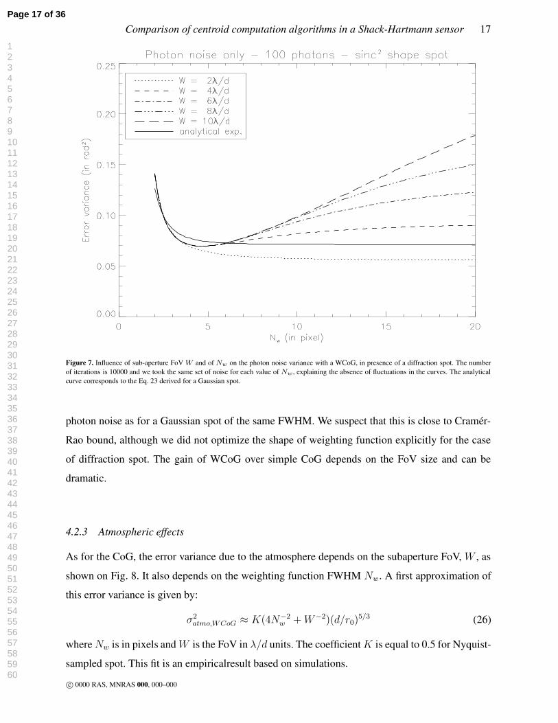
Figure 7. Influence of sub-aperture FoV W and of Nw on the photon noise variance with a WCoG, in presence of a diffraction spot. The numberof iterations is 10000 and we took the same set of noise for each value of Nw , explaining the absence of fluctuations in the curves. The analyticalcurve corresponds to the Eq. 23 derived for a Gaussian spot.

photon noise as for a Gaussian spot of the same FWHM. We suspect that this is close to Cramer-

Rao bound, although we did not optimize the shape of weighting function explicitly for the case

of diffraction spot. The gain of WCoG over simple CoG depends on the FoV size and can be

dramatic.

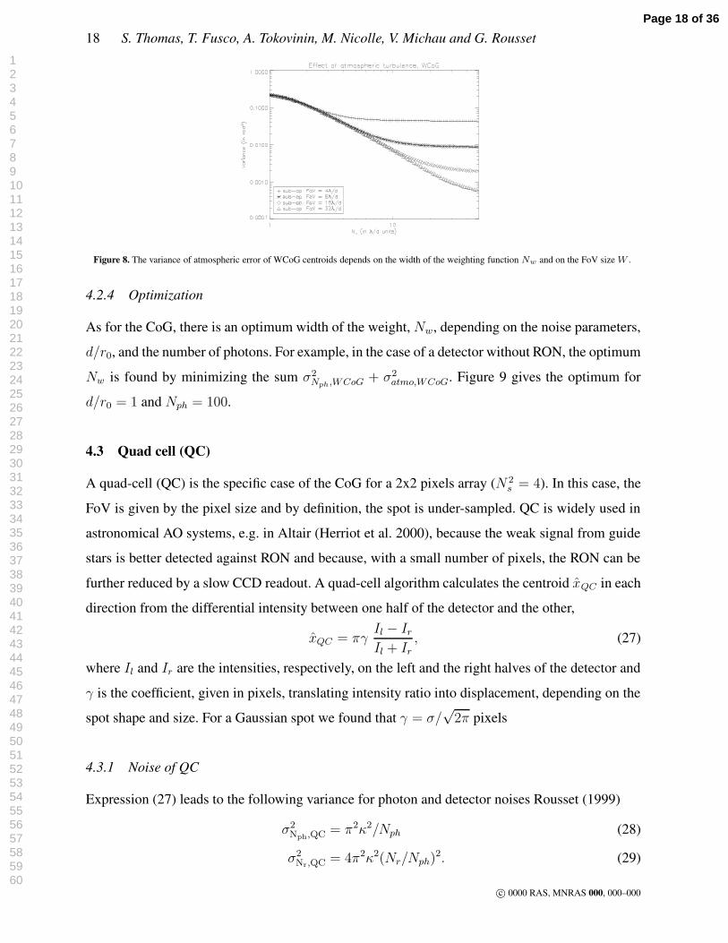
4.2.3 Atmospheric effects

As for the CoG, the error variance due to the atmosphere depends on the subaperture FoV, W , as

shown on Fig. 8. It also depends on the weighting function FWHM Nw. A first approximation of

this error variance is given by:

σ2atmo,WCoG ≈ K(4N−2

w + W−2)(d/r0)5/3 (26)

where Nw is in pixels and W is the FoV in λ/d units. The coefficient K is equal to 0.5 for Nyquist-

sampled spot. This fit is an empiricalresult based on simulations.

c© 0000 RAS, MNRAS 000, 000–000

Page 17 of 36

123456789101112131415161718192021222324252627282930313233343536373839404142434445464748495051525354555657585960


Figure 8. The variance of atmospheric error of WCoG centroids depends on the width of the weighting function Nw and on the FoV size W .

4.2.4 Optimization

As for the CoG, there is an optimum width of the weight, Nw, depending on the noise parameters,

d/r0, and the number of photons. For example, in the case of a detector without RON, the optimum

Nw is found by minimizing the sum σ2Nph,WCoG + σ2

atmo,WCoG. Figure 9 gives the optimum for

d/r0 = 1 and Nph = 100.

4.3 Quad cell (QC)

A quad-cell (QC) is the specific case of the CoG for a 2x2 pixels array (N 2s = 4). In this case, the

FoV is given by the pixel size and by definition, the spot is under-sampled. QC is widely used in

astronomical AO systems, e.g. in Altair (Herriot et al. 2000), because the weak signal from guide

stars is better detected against RON and because, with a small number of pixels, the RON can be

further reduced by a slow CCD readout. A quad-cell algorithm calculates the centroid xQC in each

direction from the differential intensity between one half of the detector and the other,

xQC = πγIl − Ir

Il + Ir

, (27)

where Il and Ir are the intensities, respectively, on the left and the right halves of the detector and

γ is the coefficient, given in pixels, translating intensity ratio into displacement, depending on the

spot shape and size. For a Gaussian spot we found that γ = σ/√

2π pixels

4.3.1 Noise of QC

Expression (27) leads to the following variance for photon and detector noises Rousset (1999)

σ2Nph,QC = π2κ2/Nph (28)

σ2Nr,QC = 4π2κ2(Nr/Nph)

2. (29)

c© 0000 RAS, MNRAS 000, 000–000

Page 18 of 36

123456789101112131415161718192021222324252627282930313233343536373839404142434445464748495051525354555657585960


Figure 9. Trade-off for the FHWM of the weighting function. Photon-noise (dashed line) and atmospheric (dotted line) variances are plotted as afunction of Nw (in pixels) for the following conditions: d/r0 = 1, Nph = 100 and W = 8λ/d. The variance sum (solid line) shows a minimumaround Nw = 7. Nyquist-sampled spot is considered.

For a diffraction-limited spot, κ = 1. For a Gaussian spot, κ depends on the rms size of the spot.

Following our definition for a Gaussian spot, the rms size is defined by σ and is given in radians

in this case (and in this paper for this case only). Therefore κ = γ 2π/(λ/d) =√

2π σ/(λ/d).

In real AO systems γ is usually variable, and considerable effort has been invested in developing

methods of real-time QC calibration (Veran & Herriot 2000).

In the following, we will assume that we are able to correct for γ fluctuations, e.g. the rms

size fluctuations. In our simulation, the estimation of γ has been made by first calculating the

long-exposure PSF and then do linear fitting by Fourier method in order to get σ.

It is also interesting to note that nowadays, detectors in SHWFS can be photon-noise limited.

In that case, the error variance ratio of the QC and the simple CoG is:

σ2Nph,QC

σ2Nph,CoG

= 2ln2 (

√2π

2√

2ln2)2 =

π

2. (30)

The QC’s error variance is 1.57 times greater than the simple CoG’s one.

c© 0000 RAS, MNRAS 000, 000–000

Page 19 of 36

123456789101112131415161718192021222324252627282930313233343536373839404142434445464748495051525354555657585960


Figure 10. Atmospheric error variance of QC centroids: simulations (symbols) and models (lines).

4.3.2 Non-linearity of QC

The response of the QC algorithm is non-linear. Elementary calculation for a Gaussian spot leads

to β = −1/σ2spot. Hence, the non-linearity centroid error (in pixels) is σNL =

√15 σspot(σt/σspot)

3

(cf. eq. 8) It may quickly dominate other error sources even at moderate Nph. On top of that, if the

FoV size becomes smaller than the spot, additional non-linearity appears, similar to simple CoG.

4.3.3 Atmospheric noise

As for the previous algorithms, we study the atmospheric component of QC noise by ignoring

both RON and photon-noise contributions, as well as any residual spot motion. Figure 10 shows

the error variance as a function of d/r0 for different FoV. A fit of the data leads to the following

expression:

σ2φ,Atm ≈ KW (d/r0)

5/3, (31)

with KW depending on the FoV. When the FoV is very small, the error is higher (KW = 0.2)

because the spot is truncated. At larger FoV, the error variance saturates at KW = 0.07. This

model, however, works only for low turbulence, d/r0 < 1. As we see in Fig. 10, the dependence

on d/r0 becomes steeper than 5/3 power under strong turbulence. One explanation comes from the

noise of γ’s fluctuations when d/r0 > 1.

The atmospheric error barely depends on the FoV size (as soon as it is larger than a few λ/d).

Even in the low-turbulence case (KW = 0.07), it is 1.4W 2 times larger than for simple CoG (cf.

Eq. 16). In conclusion, using QC centroiding is only efficient for a noisy detector under low-flux

conditions and considering small d/r0 values. For accurate wavefront measurement and photon-

noise-limited detectors other CoG methods are better.

c© 0000 RAS, MNRAS 000, 000–000

Page 20 of 36

123456789101112131415161718192021222324252627282930313233343536373839404142434445464748495051525354555657585960


5 CORRELATION ALGORITHM

The use of the correlation in imagery is not new and has been already proposed for AO systems

that use extended reference objects, e.g. in solar observations (Rimmele & Radick 1998; Michau

et al. 1992; Keller et al. 2003; Poyneer et al. 2003). In this study, we apply correlation algorithm

(COR) to a point source. First, we compute the cross-correlation function (CCF) C between the

spot image I and some template Fw.

C(x, y) = I ⊗ Fw =∑

i,j

Ii,jFw(xi + x, yj + y) (32)

and then determine the spot center from the maximum of C(x, y). The methods of finding this

position are discussed below. Since the COR method is not based on the centroid calculation, it

appears to be very good at suppressing the noise from pixels outside the spot. Moreover, corre-

lation is known to be the best method of signal detection (“matched filtering”). We note that the

coordinates x, y are continuous, unlike discrete image pixels, hence C(x, y) can be computed with

arbitrarily high resolution.

A correlation template Fw(x, y) can be either a mean spot image, some analytical function or

the image in one subaperture, like in solar AO systems (Keller et al. 2003).

In practice, the CCF has been calculated using Fourier Transform (FT). In that case, the image

has to be put in a support at least twice as big as the image size to avoid aliasing effects. The

sampling of the computed CCF can be made arbitrarily fine. One way to do this is to plunge the

FT product into a grid Ke times larger, where Ke is the over-sampling factor.

The behavior of correlation centroiding with respect to the image sampling is not different

from other centroid methods. At low flux – for example Nph = 30 for Nr = 3e− – it is slightly

better to use Nsamp = 1.5. However, for higher flux, under-sampling (Nsamp < 2) leads to a worse

error variance, while for over-sampling (Nsamp > 2) the error variance stays the same.

We remind the reader that NT is the FWHM of the spot image, Nw the FWHM of the template

Fw. Furthermore, we will call δ the FWHM of CCF.

5.1 Determination of the CCF peak

Once the CCF is computed, it is not trivial to determine the precise position of its maximum xcorr.

To do this, we studied three methods: simple CoG with threshold (Noel 1997), parabola fitting and

Gaussian fitting.

For the thresholding method, xcorr is computed by Eq. 19 where I is replaced by C and IT by

CT = Tcorr max(C). The value of Tcorr has been optimized in parallel with Ke. Figure 11 shows

c© 0000 RAS, MNRAS 000, 000–000

Page 21 of 36

123456789101112131415161718192021222324252627282930313233343536373839404142434445464748495051525354555657585960


Figure 11. Error variance of xcorr determined by estimation of correlation maximum using a thresholded center of gravity with Gaussian shapespots (with FWHM = 2 pixels). The spot motion is 0.1 pixel rms. Both photon and readout (Nr = 3) noises are considered. Various values ofthreshold are used. The template image is a noise-free Gaussian (P(x)).

the behavior of the error variance for different thresholds (from T = 0 or T = 0.9).

For the parabola fitting, the determination of xcorr was done separately in x and y. Three points

around the maximum x∗, y∗ of C along either x or y define a parabola, and its maximum leads to

the xcorr estimate (Poyneer et al. 2003) as

xcorr = x∗ −0.5[C(x∗ + 1, y∗) − C(x∗ − 1, y∗)]

C(x∗ + 1, y∗) + C(x∗ − 1, y∗) − 2C(x∗, y∗). (33)

In this case, a resampling of Ke = 4 is necessary and sufficient. For the Gaussian fitting, the

one-dimensional cut through the maximum C(x∗, y∗) is fitted by a Gaussian curve to find xcorr.

We found that all methods of peak determination are almost identical and linear (Fig. 12) when

using a Gaussian spot.

However, while the determination of the correlation peak using a few pixels around the maxi-

mum position is the best method to use in presence of readout noise, it is not the case in presence

of atmospherical turbulence. In this latest case, information contained in the wings of the CCF is

important as well. For this reason, the methods using a given function fit, such as the parabola

fitting, will not be optimum.

The thresholding method on the other hand can be optimized by adapting the threshold value

in function of the dominant noise. If the readout noise is dominant, we will use a high value of

threshold to be sensitive only to the information contained in the peak. If the atmospherical noise

is dominant, we will use a very low threshold to also be sensitive to the information contained in

the wings of the CCF and therefore the image itself.

Thus, for comparison with other centroid algorithms, we will use the thresholding method with

a adaptable threshold.

c© 0000 RAS, MNRAS 000, 000–000

Page 22 of 36

123456789101112131415161718192021222324252627282930313233343536373839404142434445464748495051525354555657585960


Figure 12. Comparison of three different cases of peak determination for a Gaussian spot: the thresholding, the parabola fitting and the Gaussianfitting. All methods use an oversampling factor Ke = 8. There is photon noise and readout noise (Nr = 3). The theory corresponds to the sum ofEq.C7 and Eq.35.

5.2 Noise of correlation centroiding

It is possible to derive a theoretical expression of the error variance for the correlation method.

The derivation in presence of readout noise is given in Appendix C (Michau et al. 1992).

A simplified expression of Eq. C7 is:

σ2x,COR,Nr

=4δ2N2

r

N2ph

, (34)

where δ is the FWHM of C〈Fw〉, the autocorrelation function of Fw. σ2x,COR,Nr

is given in pixels2.

The photon noise derivation is more complex, we studied is by simulation only. Fig. 13 shows

the behavior of the correlation error variance in presence of photon noise only. A fit of the curve

corresponding to the best thresholding gives:

σ2x,COR,NPh

≈ π2

2 ln(2)Nph

(

NT

Nsamp

)2

(35)

This expression is equivalent to the error variance found in presence of photon noise only for the

simple CoG. It can be shown (Cabanillas 2000) that the correlation is similar to the CoG, the

optimal centroid estimator (Maximum likelihood) for a Gaussian spot in presence of photon noise

only, if the template is the logarithm of the same Gaussian Fw. We found however that using the

Gaussian distribution or the logarithm of this distribution gives very similar results.

5.3 Response coefficient and non-linearity

The response coefficient of COR used with any of the optimized peak determination methods is

equal to 1. Moreover, the linearity is very good, even when using the thresholding. Indeed, C(x, y)

is a function which can be resampled, as explained before. This allows to increase the value of the

threshold to select only the region very close to the maximum without considering only one pixel.

c© 0000 RAS, MNRAS 000, 000–000

Page 23 of 36

123456789101112131415161718192021222324252627282930313233343536373839404142434445464748495051525354555657585960


Figure 13. Error variance as a function of the number of photons for the correlation method, in presence of photon noise only, for different thresholdvalues. The spot and template are Gaussian.

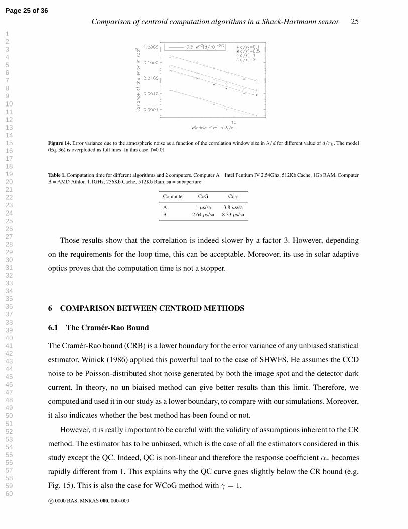
5.4 Atmospheric noise

In this section, we study the behavior of the correlation method in function of the size of the

window used in the CCF peak determination Wcor and the FWHM of the template, in presence of

atmospheric turbulence only. The CCF peak is determined by thresholding with T = 0.01, which

is the best method in this particular case; it gives lower errors at high flux. It is important to also

notice that using the thresholding method to determine the CCF peak allows the adaptation of the

threshold value depending on the flux and readout noise. Hence, the results are more accurate than

for other CCF peak determination method for any flux.

We find the same dependence of the error variance on the window size Wcor and the strength

of the turbulence as for the simple CoG, which is:

σ2φ,cor,Atm = KWcor

−2(d/r0)5/3. (36)

A fit to the data of Fig. 14 gives K ' 0.5 for well-sampled spots (Nsamp = 2). These results are

valid as long as the correlation function is not truncated (due to a high threshold for example). This

K value depends obviously on the method used to determine the peak position of the correlation

function. For example, the parabolic fitting is worse than the thresholding with a low threshold by

a factor 2. Indeed, the parabolic fitting take into account only the few pixels around the maximum.

We saw in section 5.1 that this was not the optimum method.

The main conclusion here is that in presence of only atmospheric turbulence, the correlation

method is identical to the CoG.

5.5 Computation time

We did some timing test for the CoG and the correlation for two different type of computer. The

results are given in table 1.

c© 0000 RAS, MNRAS 000, 000–000

Page 24 of 36

123456789101112131415161718192021222324252627282930313233343536373839404142434445464748495051525354555657585960


Figure 14. Error variance due to the atmospheric noise as a function of the correlation window size in λ/d for different value of d/r0. The model(Eq. 36) is overplotted as full lines. In this case T=0.01

Table 1. Computation time for different algorithms and 2 computers. Computer A = Intel Pentium IV 2.54Ghz, 512Kb Cache, 1Gb RAM. ComputerB = AMD Athlon 1.1GHz, 256Kb Cache, 512Kb Ram. sa = subaperture

Computer CoG Corr

A 1 µs/sa 3.8 µs/saB 2.64 µs/sa 8.33 µs/sa

Those results show that the correlation is indeed slower by a factor 3. However, depending

on the requirements for the loop time, this can be acceptable. Moreover, its use in solar adaptive

optics proves that the computation time is not a stopper.

6 COMPARISON BETWEEN CENTROID METHODS

6.1 The Cramer-Rao Bound

The Cramer-Rao bound (CRB) is a lower boundary for the error variance of any unbiased statistical

estimator. Winick (1986) applied this powerful tool to the case of SHWFS. He assumes the CCD

noise to be Poisson-distributed shot noise generated by both the image spot and the detector dark

current. In theory, no un-biaised method can give better results than this limit. Therefore, we

computed and used it in our study as a lower boundary, to compare with our simulations. Moreover,

it also indicates whether the best method has been found or not.

However, it is really important to be careful with the validity of assumptions inherent to the CR

method. The estimator has to be unbiased, which is the case of all the estimators considered in this

study except the QC. Indeed, QC is non-linear and therefore the response coefficient αr becomes

rapidly different from 1. This explains why the QC curve goes slightly below the CR bound (e.g.

Fig. 15). This is also the case for WCoG method with γ = 1.

c© 0000 RAS, MNRAS 000, 000–000

Page 25 of 36

123456789101112131415161718192021222324252627282930313233343536373839404142434445464748495051525354555657585960


Figure 15. Comparaison of different methods. Variance of the error in rad2 in presence of photon noise and readout noise (Nr = 3). The Gaussianspot moves randomly of 0.1 pixels rms in each direction. The plain line is the Cramer-Rao bound. The values of Nw and the FoV are given inλ/d for reference. If Tcorr = 0.6 for the correlation, the error variance decreases at low flux but the noise at high flux is higher. The best way istherefore to adapt the threshold as a function of the flux and noise.

6.2 Robustness at low flux

In Fig. 15 we compare centroid methods for a Gaussian spot, at different levels of flux. The upper

limit of reliable centroiding corresponds to the centroid variance equal to the rms spot size, or

phase variance of 7.1 rad2. It turns out that the most robust method is the Quad Cell, which can

give a good estimation of the spot position at 10 photons when Nr =3. We recall that detection

test has been implemented at low flux, explaining the behavior (saturation) of the curves.

6.3 Comparison for a Gaussian spot

After studying in detail centroiding methods independently, the methods are inter-compared. The

conclusions are:

• In presence of photon noise only, all methods after optimization are equivalent, with the

exception of the QC where the error variance saturates at high flux due to the non-linearity. The

motion of the spot is 0.1 pixel rms, leading to a non-linearity component equal to about 5 10−4

rad2.

• In presence of both readout and photon noise however, the best method depends on the flux,

as shown in Fig. 15. At low flux, the QC is the optimum method. Then, its error variance saturates

at around 5 10−4 rad2 for higher flux. At higher flux, the photon noise dominates and all methods

except the QC are identical. Fig. 15 shows a comparison with the CRB as well. The sampling is

equal to Nsamp = 2, which is the optimum for all methods at high flux. At low flux, Nsamp = 1.5

gives only marginally better results, which explains why we did not consider this value.

c© 0000 RAS, MNRAS 000, 000–000

Page 26 of 36

123456789101112131415161718192021222324252627282930313233343536373839404142434445464748495051525354555657585960


Table 2. Parameters of the study. Note that the minimum number of photons is lower for PF because of the lower detector RON value for thissystem.

d/r0 Nr Nph Nsamp

PF 1 0.5 [2-104] 2SAM 2 5 [10-104] 1

It is possible to adapt the values of the different method’s parameter as a function of flux

and readout noise to get lower error variances. In the following, we used this adaptation in the

comparison of the different methods in presence of atmospherical turbulence.

6.4 Example of results for real AO systems

Considering the high number of parameters of this study, using one method with one set of param-

eters only is an utopia. The solution is to adapt the parameters of each method depending on the

turbulence strength, the readout noise and the flux.

We will give a comparison of performance for two real systems, Planet Finder (PF) (Fusco et

al. 2005) and the SOAR Adaptive Module (SAM) (Tokovinin et al. 2004), working in two different

configurations (Table 2). PF is a second generation extreme AO for the VLT and SAM is an AO

being built for the SOAR telescope using the Ground Layer AO concept.

The first example (PF) almost can be assimilated to the case of photon noise only, which can

be reached by using a new type of CCD detectors with internal multiplication, L3CCD (Basden

et al. 2003). As said in section 3.4, the expected noise is then doubled since equivalent to what

would be found with half the flux for conventional CCD. The second example (SAM) shows the

case of common detectors where both photon and readout noise are present. The last difference is

the sampling: Nyquist for PF and half-Nyquist for SAM. For each case, we compared the different

methods described before, adapting their parameters in order to reach the best performance.

We will first comment on the detectability limit. Just as a reminder, the detectability limit is

calculated from the occurence of the maximum signal being higher than 2Nr over 1000 iterations

(c.f section 2.4. Here we will show the limit for which the maximum signal is lower than 2Nr

at least once. To give an idea for SAM, the maximum intensity of an average image is equal to

about 8% of the total flux when Nyquist sampled and 14% when half Nyquist sampled (assuming

that the center of the spot is in between 4 pixels). We then conclude that for Nph,min = 70, the

maximum intensity of the spot is too low compared to the readout noise, and all methods relying

on this maximum (like the thresholding) are useless. This limit is equal to Nph,min = 8 for the case

c© 0000 RAS, MNRAS 000, 000–000

Page 27 of 36

123456789101112131415161718192021222324252627282930313233343536373839404142434445464748495051525354555657585960


Figure 16. PF: Variance of the error in rad2 in presence of the atmospheric turbulence (d/r0 = 1) for different centroid methods. Only photonnoise is considered. The vertical dotted line (Nph = 8) represents the limit for which the signal in the brightest pixel is always greater than 2Nr .The correlation method gives the same results as the WCoG when the same paramters are used.

of PF. The values of Nph,min decrease to a few photons for FP and to about 20 photons when we

set the purcentage of occurence to 50%.

In the following we will concentrate on the WCoG, the correlation and the QC. On the figures,

we disgarded thresholding and simple CoG to avoid confusion. Those two methods are not optimal

at low flux and similar to correlation and WCoG at high flux.

Case of PF. Without RON (Fig. 16), all method are equivalent except the QC, as expected.

Considering the computation time down-side of the correlation, it is better to use the simple or

weighted CoG.

The vertical dotted line (Nph = 8) represents the limit for which the signal in the brightest

pixel is always greater than 2Nr. If the signal happens to be lower for one iteration, we remind

that the measure is not taking into account (see section 2.4).

Case of SAM. If the RON increases (Fig. 17), the results do not change when the number

of photons is high enough – NPh > 300 for Nr = 5 – since the error variance is limited by the

atmospheric turbulence.

To reduce the impact of the noise, we used a positivity constraint (use a theshold such as

T = 0) on the images before applying any method.

For low flux, the QC is 1.5 times better, assuming the optimistic case where the FWHM and

hence the response coefficient γ are known. This is linked to the high readout noise and the under-

sampling. The two other methods however either do not rely on the knowledge of the FWHM or

allow to measure the FWHM with accuracy since we have a direct access to the shape of spot,

which is not the case for QC. Moreover, the results are better at high flux. Therefore, if the error

budget allows it, the simplest and more reliable method, which is the WCoG, must be chosen, even

if it is not the best at low flux.

c© 0000 RAS, MNRAS 000, 000–000

Page 28 of 36

123456789101112131415161718192021222324252627282930313233343536373839404142434445464748495051525354555657585960


Figure 17. SAM: Variance of the error in rad2 in presence of atmospheric turbulence (d/r0 = 2) for SAM with a sampling of Nsamp = 1. Bothphoton and readout noise are present. The vertical dotted line (Nph = 70) represents the limit for which the signal in the brightest pixel is alwaysgreater than 2Nr .

6.5 Implementation issues

From those results, it is essential to consider the implementation issues of the WFS before making

a final choice. In the following we will give some comments for the different methods.

• The QC. The advantage of this method is the low number of pixels (only 2 × 2), even if in

practice we often use more pixels. However, there is an unknown which is the exact FWHM of the

spot in presence of turbulence. This FWHM must be known to get a response coefficient γ = 1.

Considering the poor sampling of the image, it is difficult to calculate the spot size from the data.

Moreover, this method is non-linear. The QC method can be interesting though in case of a very

high readout noise and small values of d/r0.

• The CoG and its improvements. The subaperture field is typically of 6 × 6 or 8 × 8 pixels.

The pure CoG is very sensitive to noisy pixels when the signal is low compared to the readout

noise or when the turbulence is high. Improvement can be achieved by optimizing the threshold

or by using a WCoG. The last one gives the best results when adapting the rms size of the Fw as a

function of flux and readout noise.

Moreover, the response coefficient γ depends on the FWHM of the spot like for the QC. How-

ever, in that case it will be easier to determine γ since we have a direct measurement of the spot.

The procedure will be to recenter and average off-line individual frames in order to obtain a re-

centered long exposure image and then derive the FWHM value from this direct data. Then, this

value of FWHM will be used in the next measurement.

• The correlation. The computation for this method is more complex, especially when over

sampling is needed to estimate the peak position of the correlation function. The thresholded CoG

gives the best estimation of the peak position of the correlation function, since the adaptation

c© 0000 RAS, MNRAS 000, 000–000

Page 29 of 36

123456789101112131415161718192021222324252627282930313233343536373839404142434445464748495051525354555657585960


of the threshold allows to deal with either high readout noise or high atmospheric turbulence.

Other methods are not as robust and give higher error in presence of atmospheric turbulence. The

advantage of COR is that the response coefficient does not depend on the spot size and shape.

7 CONCLUSIONS AND FUTURE WORK

In this paper, we gave a practical comparison of different methods of centroid calculation in a

Shack-Hartmann wavefront sensor. We studied some variations of the center of gravity such as

WCoG, thresholding and quad cell. We also considered the use of the correlation to determine

the spot positions. The first part of the paper was focused on the simplified case of Gaussian spot

or diffraction-limited spot without atmospheric turbulence, while the second part considered all

sources of error.

We are not presenting here a real recipe but a methodology to calculate the error of a SH

wavefront sensor. This study can be applied to different domains by changing the parameters and

the shape of the spot.

We first show a good understanding of the theory in the case of a Gaussian spot. For this

particular case, the formulae can be used directly to estimate the noise in the WFS.

For diffraction-limited spot and spots distorted by atmospheric turbulence, the derivation of

such formulae is more challenging. Therefore, we have studied the methods mainly by simulation.

The comparison is given in two different cases: with and without readout noise for a strength of

turbulence equal to d/r0 = 2. The best method would be the WCoG, with adapting the size of the

weighting function, which does not require a complicated implementation.

The correlation gives also good results and good detectability by adapting the threshold value

to the flux and the RON considered. One can notice as well that at high flux, the correlation

and the simple CoG give smallest errors and are similar. It is safe to say that for point sources the

correlation method is not worth using, considering the complexity of its implementation. However,

in presence of elongated spots it is the best method (Poyneer et al. 2003). We are planning to

continue this study.

For lower turbulence, the QC is very efficient for high readout noise and leads to simpler

detectors.

The conclusion though is that we do not have a magic method. However, the WCoG gives

the optimum results independently of the signal to noise ratio when adjusting the FWHM of the

weighting function. The study was made in the context of detailed designs and trade-offs where

c© 0000 RAS, MNRAS 000, 000–000

Page 30 of 36

123456789101112131415161718192021222324252627282930313233343536373839404142434445464748495051525354555657585960


simplified analytical formula do not apply in the prediction of the WFS behavior. We also show

the complexity of the problem and the importance of the contribution of each error in the budget

for the comparison of different methods (or more generally different type of WFS).

ACKNOWLEDGEMENTS

This study has been financed by NOAO. We thank Lisa Poyneer and Rolando Cantarutti for useful

discussions. Jean-Marc Conan and Laurent Mugnier as well were very helpful in this study.

APPENDIX A: PHOTON NOISE EXPRESSION IN THE CASE OF A DIFFRACTION

LIMITED SPOT

In the case of a diffraction limited spot and a Poisson statistics (photon noise case), the eq. 11 is

no longer valid. Indeed, there is some signal contained in the wings of the PSF leading to photon

noise. The size of the window has to be optimized. The photon noise variance (for one direction)

can be expressed for this case as

σ2φ,Nph

=

(

2πd

λ

)21

N2ph

∫ w/2

−w/2

∫ w/2

−w/2

α2〈P 2(α, β)〉dαdβ (A1)

with P (α, β) the sinc2 shape of the spot (cf Eq. 2) and w the size of the subaperture in radians.

Because we are in presence of photon noise only in this case, 〈P 2(α, β)〉 = P (α, β) and therefore

we can write:

σ2φ,Nph

=

(

2πd

λ

)21

Nph

∫ w/2

−w/2

α2sinc2

(

α

λ/d

)

dα

∫ w/2

−w/2

sinc2

(

β

λ/d

)

dβ. (A2)

We have∫ w/2

−w/2

α2sinc2

(

α

λ/d

)

dα = 2λ2

(πd)2

∫ w/2

0

sin2

(

πdα

λ

)

dα

=

(

λ

πd

)2w

2

[

1 − sinc

(

dw

λ

)]

, (A3)

and∫ w/2

−w/2

sinc2

(

β

λ/d

)

dβ =λ

πd

∫ πdλ

w2

0

sinc2 (γ) dγ, (A4)

where, γ = βλ/d

.

c© 0000 RAS, MNRAS 000, 000–000

Page 31 of 36

123456789101112131415161718192021222324252627282930313233343536373839404142434445464748495051525354555657585960


Thus,

σ2φ,Nph

=

(

2πd

λ

)21

Nph

(

λ

πd

)2w

2

[

1 − sinc

(

dw

λ

)]

λ

πd

∫ πdλ

w2

0

sinc2 (γ) dγ, (A5)

The function[

1 − sinc(

πdwλ

)]

tends to 1 (with some oscillations) and∫ πd

λw2

0sinc2(γ) dγ tends

to π/2 when w tends to infinity (or at least if w >> λd

). In that case, Eq. A5 can be approximated

by

σ2φ,Nph

≈(

2πd

λ

)21

Nph

w

2

(

λ

πd

)3

π ≈ 2W

Nph

, (A6)

with W = wλ/d, the size of the subaperture in λ/d unit.

APPENDIX B: DERIVATION OF THE COG ESTIMATE CALCULATED ON A FINITE

WINDOW

The definition of the center of gravity of P (x, y) on a finite window of size Wp is:

x =1

P0

∫∫ Wp/2

−Wp/2

x P (x, y) dx dy, (B1)

with

P0 =

∫∫ Wp/2

−Wp/2

P (x, y) dx dy (B2)

=

∫∫ Wp/2

−Wp/2

Nph

2πσ2spot

e−((x−x0)2+y2)/2σ2

spot dx dy (B3)

=Nph

2πσ2spot

∫ Wp/2

−Wp/2

e−(x−x0)2/2σ2

spot dx (B4)

∫ Wp/2

−Wp/2

e−y2/2σ2spot dy. (B5)

We first get by deriving the expression of I0

P0 =Nph

2[ Φ (η) + Φ (ζ)] × Φ

(

Wp/2

σspot

√2

)

(B6)

where ζ = (Wp/2−x0)/(√

2σspot), η = (Wp/2−x0)/(√

2σspot), and Φ(t) = 2/√

π∫ t

0exp(−u2) du.

c© 0000 RAS, MNRAS 000, 000–000

Page 32 of 36

123456789101112131415161718192021222324252627282930313233343536373839404142434445464748495051525354555657585960


Then from Eq.B1, we obtain:

x =1

P0

∫∫ Wp/2

−Wp/2

xNph

2πσ2spot

e−

(x−x0)2+y2

2σ2spot dx dy (B7)

=1

P0

∫ Wp/2

−Wp/2

x e−(x−x0)2/2σ2

spot dx (B8)

∫ Wp/2

−Wp/2

e−y2/2σ2spot dy. (B9)

This leads to:

x = x0 − σspot

√

2

π

eζ − eη

Φ(ζ) + Φ(η). (B10)

The derivation for the WCoG is similar, taking:

x =1

P0

∫∫ Wp/2

−Wp/2

x P (x, y)Fw (x, y) dx dy (B11)

where Fw is the weighting function, and

P0 =

∫∫ Wp/2

−Wp/2

P (x, y)Fw (x, y) dx dy. (B12)

APPENDIX C: READOUT NOISE CALCULATION FOR THE CORRELATION

METHOD

Here, we consider the case where the reference Fw is a known, deterministic function. Let’s s be

the threshold and D the domain where C(x, y) > s, and Dc the domain where the functions are

defined. Then

xcorr =

∫

Dx [C(x, y) − s] dxdy

∫

D[C(x, y) − s] dxdy

=Ng

Dg

, (C1)

where Ng is the numerator and Dg the denominator. If we assume that the fluctuations of Dg are

negligible compared to those of Ng, we find that:

σ2x,COR =

〈N2g 〉 − 〈Ng〉2〈Dg〉2

, (C2)

where

〈N2g 〉 − 〈Ng〉2 =

∫

D

∫

D

xx′σ2C(x, y, x′, y′)dxdydx′dy′, (C3)

where σ2C(x, y, x′, y′) is the variance of the correlation function. We can show that

σ2C(x, y, x′, y′) =∫

Dc

∫

Dc

Fw(u, v)Fw(u′, v′) [〈I(u + x, v + y)I(u′ + x′, v′ + y′)〉

− 〈I(u + x, v + y)〉〈I(u′ + x′, v′ + y′)〉] dudvdu′dv′. (C4)

c© 0000 RAS, MNRAS 000, 000–000

Page 33 of 36

123456789101112131415161718192021222324252627282930313233343536373839404142434445464748495051525354555657585960


Since

[〈I(x, y)I(x′, y′)〉 − 〈I(x, y)〉〈I(x′, y′)〉] =

σ2b (x, y), if (x, y) = (x′, y′)

0, if (x, y) 6= (x′, y′)(C5)

where σb(x, y) is the noise density. In presence of readout noise, which is a white noise, σb is

a constant equal to Nr.

σ2C(x, y, x′, y′) = N2

r

∫

Dc

Fw(u, v)Fw(u + x − x′, v + y − y′)dudv (C6)

Therefore, a development of Eq. C2 gives:

σ2x,COR,Nr

= N2r

∫

D

∫

Dxx′[

C〈Fw〉(x − x′, y − y′)]

dxdydx′dy′

〈Dg〉2, (C7)

where C〈Fw〉 is the autocorrelation function of Fw. σ2x,COR,Nr

is given in pixels2.

A simplified expression of Eq. C7 can be derived using the following approximation:

C〈Fw〉(x, y) ≈ CI(x, y)(Dc ⊗ Dc)(x, y) (C8)

close to the maximum. Then, we can fit the function near the maximum by a parabola as:

CI(x, y) = N2ph

(

1 − x2 + y2

2δ2

)

(C9)

where δ is the FWHM of C〈Fw〉.

We finally find

σ2x,COR,Nr

=4δ2N2

r

N2ph

. (C10)

REFERENCES

Arines J., Ares J., 2002, Opt. Let., 27, 497

Basden A. G., Haniff C. A., Mackay C. D., 2003, MNRAS, 345, 985

Blanc A., Fusco T., Hartung M., Mugnier L. M., Rousset G., 2003, A&A, 399, 373

Cabanillas S., 2000, Thesis from Aix-Marseille University

Esposito S. , Riccardi A., 2001, A&A, 369, L9

Fusco T., Nicolle M., Rousset G., Michau V., Beuzit J.-L., Mouillet D., 2004, Proc. SPIE, 5490,

p. 1155

Fusco T., Rousset G., Beuzit J.-L., Mouillet D., Dohlen K., Conan R., Petit C., Montagnier G.,

2005, Proc. SPIE, 5903, p.148

Gendron E. et al., 2005, C. R. Physique 6, in press

Guillaume M., Melon P., Refregier P., Llebaria A., 1998, J.Opt.Soc.Amer(A), 15, p.2841

c© 0000 RAS, MNRAS 000, 000–000

Page 34 of 36

123456789101112131415161718192021222324252627282930313233343536373839404142434445464748495051525354555657585960


Hardy J.W., Adaptive Optics for Astronomical Telescope, 1998, Oxford University Press, p.147

Hartung M. , Blanc A., Fusco T., Lacombe F., Mugnier L. M., Rousset G., Lenzen R., 2003,

A&A, 399, 385

Herriot G., Morris S., Anthon A., 2000, Proc. SPIE, 4007, p. 115

Irwan R., Lane R. G., 1999, Appl. Opt., 38, 6737

Keller Ch. U., Plymate C., Ammons S.M., 2003, Proc. SPIE, 4853, p. 351

Madec P.Y., 1999, in F. Roddier, ed., Adaptive optics in Astronomy. Cambridge University press,

p. 131

Michau V., Rousset G., Fontanella J.C., 1992, in Real time and post facto solar image correction,

Sunspot, New Mexico, p. 124

Nicolle M., Fusco T., Rousset G., Michau V., 2004, Opt. Let., 29, 2743

Noel T., 1997, Thesis ONERA, Paris

Noll R.J., 1976, J.Opt.Soc.Amer(A), 66, p. 207

Poyneer L. A., LaFortune K., Awwal A.A.S., 2003, Lawrence Livermore National Lab Report

(Livermore, CA 94551)

Ragazzoni, R., Farinato, J., 1999, A&A, 350, L23

Rimmele T. R., Radick R. R., 1998, Proc. SPIE, 3353, p.72

Rousset G., 1999, in F. Roddier, ed., Adaptive optics in Astronomy, Cambridge University press,

p.115

Rousset G., Lacombe F., Puget P., Hubin N. N., Gendron E., Fusco T., Arsenault R., Charton J.

et al., 2003, Proc. SPIE, 4839, p. 140

Ruggiu J.-M., Solomon C. J.,Loos G., 1998, Opt. Let., 23, 235

Sallberg S.A., Welsh B.M., Roggemann M.C., 1997, J.Opt.Soc.Amer(A) , 14, 1347

Sandler D., 1999, in F. Roddier, ed., Adaptive optics in Astronomy. Cambridge University press,

p.294

Sasiela R.J., Electromagnetic wavepropagation in turbulence, 1994, Springer-Verlag, Berlin

Sauvage J.-F., Fusco T., Rousset G., Petit C., Neichel B., Blanc A., Beuzit J.-L., 2005, Proc.

SPIE, 5903, 100

Tokovinin A., Thomas S., Gregory B., van der Bliek N., Schurter P., Cantarutti R., Mondaca E.,

2004, Proc. SPIE, 5490, 870

Tyler G.A., 1994, J.Opt.Soc.Amer(A), 11, 358

van Dam M. A. & Lane R. G., 2000, J.Opt.Soc.Amer(A), 17, 1319

Veran J.-P., Herriot G., 2000, J.Opt.Soc.Amer(A), 17, 1430

c© 0000 RAS, MNRAS 000, 000–000

Page 35 of 36

123456789101112131415161718192021222324252627282930313233343536373839404142434445464748495051525354555657585960


Winick K.A., 1986, J.Opt.Soc.Amer(A), 3, 1809

c© 0000 RAS, MNRAS 000, 000–000

Page 36 of 36

123456789101112131415161718192021222324252627282930313233343536373839404142434445464748495051525354555657585960

comparison of centroid computation algorithms in a …atokovin/papers/wfs_apr28.pdfmon. not. r....

Documents