comparison of azimuthal seismic anisotropy from surface...
TRANSCRIPT

Geophys. J. Int. (XXXX) XXX, XXX–XXX
Comparison of azimuthal seismic anisotropy from surface wavesand finite-strain from global mantle-circulation models
T.W. Becker1 � , J.B. Kellogg2, G. Ekstrom2, and R.J. O’Connell21Cecil H. and Ida M. Green Institute of Geophysics and Planetary Physics,Scripps Institution of Oceanography, University of California, San Diego, 9500 Gilman Drive, La Jolla CA 92093, USA2Department of Earth and Planetary Sciences, Harvard University, 20 Oxford Street, Cambridge MA 02138, USA
Submitted to Geophysical Journal International on January 7, 2003
SUMMARY
We present global models of strain accumulation in mantle flow to compare the pre-dicted finite-strain ellipsoid (FSE) orientations with observed seismic anisotropy. Thegeographic focus is on oceanic and young continental regions where we expect ourmodels to agree best with azimuthal anisotropy from surface waves. Finite-strain de-rived models and alignment with the largest FSE axes leads to better model fits thanthe hypothesis of alignment of fast propagation orientation with absolute plate mo-tions. Our modeling approach is simplified in that we are using a linear viscosity forflow and assume a simple relationship between strain and anisotropy. However, resultsare encouraging and suggest that similar models can be used to assess the validity of as-sumptions inherent in the modeling of mantle convection and lithospheric deformation.Our results substantiate the hypothesis that seismic anisotropy can be used as an indi-cator for mantle flow; circulation-derived models can contribute to the establishmentof a quantitative functional relationship between the two.
Key words:mantle convection – seismic anisotropy – finite strain – plate driving forces – intraplatedeformation
1 INTRODUCTION
Seismic wave propagation in the uppermost mantle isanisotropic, as has been demonstrated using a variety ofmethods and datasets (e.g. Hess 1964; Forsyth 1975; An-derson & Dziewonski 1982; Vinnik et al. 1989; Montagner& Tanimoto 1991; Schulte-Pelkum et al. 2001). Verticallypolarized waves propagate more slowly than horizontallypolarized waves in the upper � 220 km of the mantle, imply-ing widespread transverse isotropy with a vertical symme-try axis. Surface-wave studies have established lateral varia-tions in the pattern of this radial anisotropy (e.g. Ekstrom& Dziewonski 1998). Inverting for azimuthal anisotropy(where the fast propagation axis lies within the horizon-tal) is more difficult, partly because of severe trade-offs be-tween model parameters (e.g. Tanimoto & Anderson 1985;Laske & Masters 1998). Ongoing efforts to map azimuthalanisotropy in 3-D using surface waves (e.g. Montagner
& Tanimoto 1991) are reviewed by Montagner & Guillot(2000).
The existence of anisotropy in upper-mantle rocks canbe associated with accumulated strain due to mantle con-vection (e.g. McKenzie 1979), as reviewed by Montagner(1998). The use of seismic anisotropy as an indicator formantle and lithospheric flow is therefore an important av-enue to pursue since other constraints for deep mantle floware scarce. There are currently few quantitative models thatconnect anisotropy observations to the three-dimensional (3-D) geometry of mantle convection, and this paper describesour attempts to fill that gap using Rayleigh wave data andglobal circulation models.
Surface waves studies can place constraints on varia-tions of anisotropy with depth, but the lateral data resolutionis limited. Alternative datasets such as shear-wave splittingmeasurements have the potential to image smaller-scale lat-eral variations, though they lack depth resolution (e.g. Sil-ver 1996; Savage 1999). However, an initial comparisonbetween observations and synthetic splitting from surface-wave models showed poor agreement between results from

2 T.W. Becker, J.B. Kellogg, G. Ekstrom, and R.J. O’Connell
both approaches (Montagner et al. 2000). Possible reasonsfor this finding include that the modeling of shear-wave split-ting measurements needs to take variations of anisotropywith depth into account (e.g. Schulte-Pelkum & Black-man 2002). The predicted variations of finite-strain withdepth from geodynamic models can be quite large (e.g. Hallet al. 2000; Becker 2002), implying that a careful treatmentof each set of SKS measurements might be required. We willthus focus on surface-wave based observations of azimuthalanisotropy for this paper and try to establish a general un-derstanding of strain accumulation in 3-D flow. In subse-quent models, other observations of anisotropy should alsobe taken into account.
1.1 Causes of seismic anisotropy
Anisotropy in the deep lithosphere and upper mantle is mostlikely predominantly caused by the alignment of intrinsi-cally anisotropic olivine crystals (lattice-preferred orienta-tion, LPO) in mantle flow (e.g. Nicolas & Christensen 1987;Mainprice et al. 2000). Seismic anisotropy can thereforebe interpreted as a measure of flow or velocity-gradients inthe mantle and has thus received great attention as a possi-ble indicator for mantle convection (e.g. McKenzie 1979;Ribe 1989; Chastel et al. 1993; Russo & Silver 1994;Tommasi 1998; Buttles & Olson 1998; Hall et al. 2000;Blackman & Kendall 2002). There is observational (Ben Is-mail & Mainprice 1998) and theoretical (Wenk et al. 1991;Ribe 1992) evidence that rock fabric and the fast shear-wavepolarization axis will line up with the orientation of maxi-mum extensional strain. (We shall distinguish between di-rections, which refer to vectors with azimuths between 0
�and 360
�, and orientations, which refer to two-headed vec-
tors with azimuths that are 180�-periodic. We will also use
fabric loosely for the alignment of mineral assemblages inmantle rocks such that there is a pronounced spatial cluster-ing of particular crystallographic axes around a specific ori-entation, or in a well-defined plane.) More specifically, weexpect that for a general strain state, the fast (a), intermediate(c), and slow (b) axes of olivine aggregates will align, to firstorder, with the longest, intermediate, and shortest axes of thefinite strain ellipsoid (Ribe 1992). The degree to which thefast axes cluster around the largest principal axis of the fi-nite strain ellipsoid (FSE), or, alternatively, the orientationof the shear plane, will vary and may depend on the exactstrain history, temperature, mineral assemblage of the rock,and possibly other factors (e.g. Savage 1999; Tommasiet al. 2000; Blackman et al. 2002; Kaminski & Ribe 2002).The simple correlation between FSE and fabric may there-fore not be universally valid. For large-strain experiments,the fast propagation orientations were found to rotate into theshear plane of the experiment (Zhang & Karato 1995), aneffect that was caused partly by dynamic recrystallization ofgrains and that is accounted for in some of the newer theoret-ical models for fabric formation (e.g. Wenk & Tome 1999;Kaminski & Ribe 2001, 2002). Further complications forLPO alignment could be induced by the presence of water(Jung & Karato 2001).
Instead of trying to account for all of the proposedanisotropy formation mechanisms at once, we approach theproblem by using global flow models to predict the orien-tation of finite strain in the mantle. We then compare the
anisotropy produced by these strains to the seismic data, us-ing a simplified version of Ribe’s (1992) model. We focuson oceanic plates where the lithosphere should be less af-fected by inherited deformation (not included in our model)than in continental areas. The agreement between predictedmaximum extensional strain and the fast axes of anisotropyis found to be good in most regions which supports the in-ferred relationship between strain and fabric in the mantle.We envision that future, improved global circulation modelscan be used as an independent argument for the validity andthe appropriate parameter range of fabric development mod-els such as that of Kaminski & Ribe (2001), and intend toexpand on our basic model in a next step.
2 AZIMUTHAL ANISOTROPY FROM RAYLEIGHWAVES
Tomographic models with 3-D variations of anisotropybased on surface waves exist (Montagner & Tanimoto 1991;Montagner & Guillot 2000). However, since there are someconcerns about the resolving power of such models (e.g.Laske & Masters 1998), we prefer to directly compareour geodynamic models with a few azimuthally-anisotropicphase-velocity maps from inversions by Ekstrom (2001). Inthis way, we can avoid the complications that are involved ina 3-D inversion.
Phase velocity perturbations, δc, for weak anisotropycan be expressed as a series of isotropic, D0, and az-imuthally anisotropic terms with π-periodicity, D2φ, andπ�2-periodicity, D4φ, (Smith & Dahlen 1973):
δc � dcc � D0 � D2φ
C cos � 2φ � D2φS sin � 2φ �
D4φC cos � 4φ � D4φ
S sin � 4φ � (1)
where φ denotes azimuth. D2φ and D4φ anisotropy implythat there are one and two fast propagation orientations in thehorizontal plane, respectively. As discussed in the Appendix,fundamental mode Rayleigh waves are typically more sensi-tive to anisotropy variations with 2φ-dependence than Lovewaves; we will thus focus on Rayleigh waves.
The kernels for surface wave sensitivity to 2φ-anisotropy have a depth dependence for Rayleigh waves thatis similar to their sensitivity to variations in vSV (Montag-ner & Nataf 1986) with maximum sensitivity at � 70 km, �120 km, � 200 km depth for periods of 50 s, 100 s, and 150 s,respectively (see Appendix). Figure 1 shows phase-velocitymaps from inversions by Ekstrom (2001) for those periods.Ekstrom used a large dataset ( � 120 000 measurements) anda surface-spline parameterization (1442 nodes, correspond-ing to � 5
�spacing at the equator) to invert for lateral varia-
tions in the D terms of (1). To counter the trade-off betweenisotropic and anisotropic structure, Ekstrom (2001) damped2φ and 4φ-terms 10 times more than the isotropic D0 param-eters. The inversion method will be discussed in more detailin a forthcoming publication, and the resolving power forD2φ anisotropy will be addressed in sec. 5.1. Here, we shallonly briefly discuss some of the features of the anisotropymaps.
The isotropic and 2φ-anisotropic shallow structure im-aged in Figure 1 appears to be dominated by plate-tectonic

Seismic anisotropy and mantle flow 3
(a) T � 50 s (peak D2φ-sensitivity: 70 km depth)0˚ 60˚ 120˚ 180˚ 240˚ 300˚ 360˚
-60˚
-30˚
0˚
30˚
60˚
D4φ: 1.8%D2φ: 2.5%inversion:
-6
-4
-2
0
2
4
6
D0 [%]
(b) T � 100 s (peak D2φ-sensitivity: 120 km depth)0˚ 60˚ 120˚ 180˚ 240˚ 300˚ 360˚
-60˚
-30˚
0˚
30˚
60˚
D4φ: 2.0%D2φ: 2.9%inversion:
-4
-2
0
2
4
D0 [%]
(c) T � 150 s (peak D2φ-sensitivity: 200 km depth)0˚ 60˚ 120˚ 180˚ 240˚ 300˚ 360˚
-60˚
-30˚
0˚
30˚
60˚
D4φ: 1.7%D2φ: 2.1%inversion:
-2
0
2
D0 [%]
Figure 1. Isotropic and anisotropic variations of phase velocity for Rayleigh waves at periods, T , of 50 s (a), 100 s (b), and 150 s (c) from Ekstrom (2001).We show isotropic anomalies as background shading (D0 term in (1)), D2φ fast orientations as sticks, and D4φ terms as crosses with maximum amplitude asindicated in the legend. D2φ sensitivity peaks at � 70 km, � 120 km, and � 200 km depth for 50 s, 100 s, and 150 s, respectively (see Appendix).

4 T.W. Becker, J.B. Kellogg, G. Ekstrom, and R.J. O’Connell
50 s recovery
-0.4 -0.2 0 0.2 0.4
r
|vh | avg
|vr | avg
rum
continent
craton
seafloor_age
iso vs. D 2φ
Dr2φ
50 s
-0.4 -0.2 0 0.2 0.4
r
D0 D0vs.D2φ D2φ D4φ100 s
-0.4 -0.2 0 0.2 0.4
r
150 s
-0.4 -0.2 0 0.2 0.4
r
Figure 2. Correlation coefficient, r, for T � 50 s recovery test and surface wave models of Figure 1 at periods of 50 s, 100 s, and 150 s. We show isotropicanomaly (D0, circles), 2φ-anisotropy (D2φ amplitude, filled triangles), and 4φ-anisotropy (D4φ amplitude, squares) correlations with seafloor-age, cratons, andcontinental regionalizations (from Nataf & Ricard 1996), uppermost mantle slabs (rum, average upper 400 km from Gudmundsson & Sambridge 1998),average absolute radial ( � vr � avg) and horizontal ( � vh � avg) velocities from a flow calculation based on plate motions (upper 400 km average, no-net-rotationframe) and smean nt (sec. 3.1). Stars indicate r between the isotropic and D2φ-signal, and open triangles for the leftmost plot the correlations of surfacewave inversion’s D2φ amplitude-recovery, D2φ
r � log10 � D2φrecovered � D2φ
model � , as discussed in sec. 5.1. All fields are expanded up to spherical harmonic degree�max � 31 before calculating r; vertical dashed lines indicate the corresponding 99% significance level assuming bi-normal distributions.
features such as the well-known seafloor spreading-patternclose to the ridges (e.g. Forsyth 1975; Montagner & Tani-moto 1991). There are, however, deviations from this sim-ple signal, and the D2φ pattern in the Western Pacific andsouth-western parts of the Nazca plate has no obvious rela-tion to current plate motions. The patterns in anomaly ampli-tudes are quantified in Figure 2. We show the correlation ofD0, D2φ, and D4φ-variations with tectonic regionalizationsand plate-motion amplitudes. The isotropic signal shows apositive correlation with sea-floor age for T � 50 s, sinceridges are where slow wave-speeds are found; this signalis lost for deeper sensing phases. Especially for T � 50 s,both convergent and divergent plate boundaries are foundto be seismically slow, which is reflected in a negative cor-relation coefficient, r, with the radial velocities from flowmodels, � vr � avg. D0 is also positively correlated with cratonsfor all periods, because the continental tectosphere is gen-erally imaged as fast structure by tomography. There is anegative correlation of D0 with horizontal velocities; thisis partly the consequence of positive r with continental re-gions because oceanic plates move faster than continentalones. The D2φ-signal has a negative correlation with cratonsfor all T , and a positive correlation with horizontal and ra-dial velocities for T � 100 s. The observed weaker regionalanisotropy underneath cratons might be due to the higherviscosity of continental keels (and hence less rapid shear-ing) and/or frozen in fabric with rapidly varying orientationswhich is averaged out by the surface wave inversion. Posi-tive r for D2φ with plate speeds in turn may be caused bymore rapid shearing underneath oceanic plates. However,especially this last conclusion is weakened by the unevenraypath coverage which limits tomographic inversions. Theability of Ekstrom’s (2001) dataset to recover synthetic D2φ-structure is reflected by the correlation of the D2φ-recoveryfunction, D2φ
r , from sec. 5.1, shown in open triangles in Fig-ure 2. As a consequence of the event-receiver geometry, re-
covery of azimuthal anisotropy is better in the oceanic platesthan in the continents, which leads to a positive and nega-tive r of D2φ
r with horizontal plate speeds and the continentalfunction, respectively.
If anisotropy were purely due to a clearly defined fastpropagation axis in the horizontal plane, we would expectthe D4φ signal to be much smaller than D2φ for fundamentalmode Rayleigh waves (see Montagner & Nataf 1986, andAppendix). The 4φ-signal in Figure 1 is indeed smaller thanthat from 2φ, but it is not negligible. Both 4φ and 2φ ampli-tudes are positively correlated with plate boundaries ( � vr � avg
in Figure 2), especially with convergent margins where slabsare found (rum in Figure 2). This might indicate that thepredominantly vertical orientation of strain in these regions(sec. 3.4) causes the symmetry axis of anisotropy to have alarge radial component. However, we will proceed to inter-pret only the D2φ signal for simplicity, and compare the ob-served fast axes with the horizontal projection of the longestaxis of the flow-derived FSEs. Some of the largest deviationsbetween our models and observations are in the regions oflarge D4φ (sec. 5.2). This could be caused by either poor res-olution of the data or a breakdown of our model assumptionsabout anisotropy, or both.
3 MODELING STRAIN AND LPO ANISOTROPY
We predict seismic anisotropy by calculating the finite strainthat a rock would accumulate during its advection throughmantle flow (e.g. McKenzie 1979). Given a velocity fieldthat is known as a function of time and space, the passive-tracer method lends itself to the problem of determiningstrain as outlined below.
Seismic anisotropy and mantle flow 5
0
500
1000
1500
2000
2500
0.01 0.1 1 10 100
dept
h [k
m]
viscosity η [1021 Pas]
ηD (Hager & Clayton, 1989)
ηF (Steinberger, 2000)
ηG (Mitrovica & Forte, 1997)
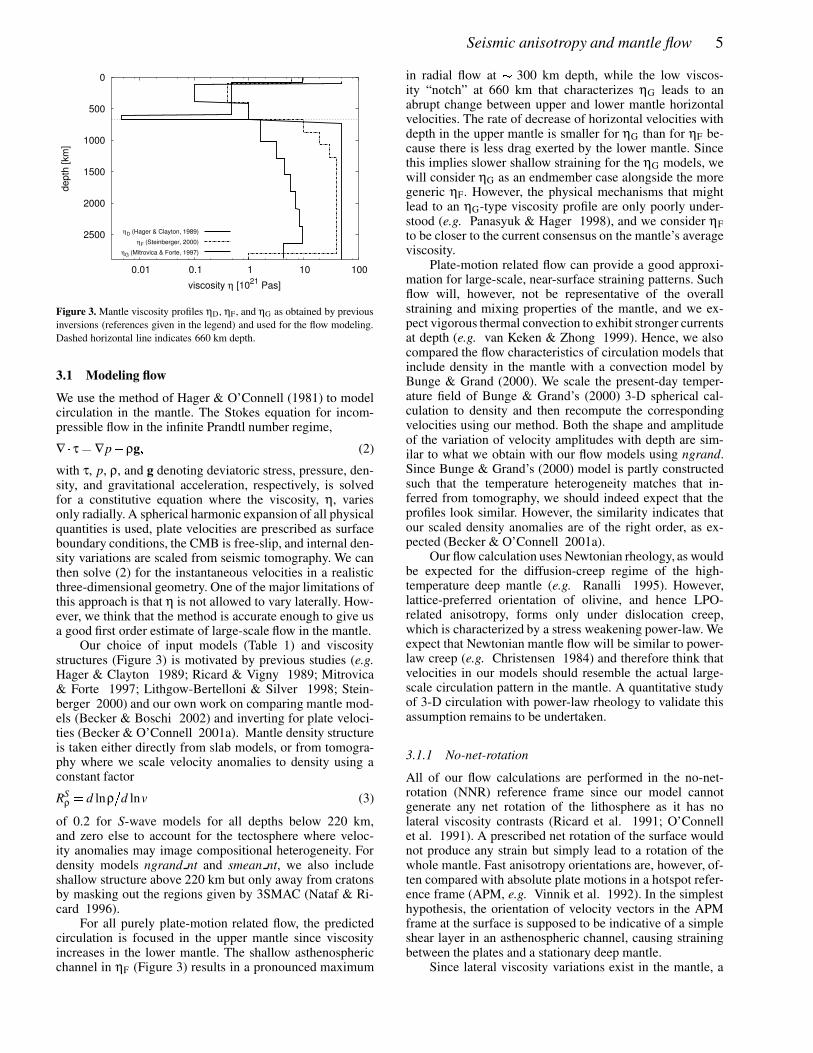
Figure 3. Mantle viscosity profiles ηD, ηF, and ηG as obtained by previousinversions (references given in the legend) and used for the flow modeling.Dashed horizontal line indicates 660 km depth.
3.1 Modeling flow
We use the method of Hager & O’Connell (1981) to modelcirculation in the mantle. The Stokes equation for incom-pressible flow in the infinite Prandtl number regime,
∇ � τ � ∇p � ρg (2)
with τ, p, ρ, and g denoting deviatoric stress, pressure, den-sity, and gravitational acceleration, respectively, is solvedfor a constitutive equation where the viscosity, η, variesonly radially. A spherical harmonic expansion of all physicalquantities is used, plate velocities are prescribed as surfaceboundary conditions, the CMB is free-slip, and internal den-sity variations are scaled from seismic tomography. We canthen solve (2) for the instantaneous velocities in a realisticthree-dimensional geometry. One of the major limitations ofthis approach is that η is not allowed to vary laterally. How-ever, we think that the method is accurate enough to give usa good first order estimate of large-scale flow in the mantle.
Our choice of input models (Table 1) and viscositystructures (Figure 3) is motivated by previous studies (e.g.Hager & Clayton 1989; Ricard & Vigny 1989; Mitrovica& Forte 1997; Lithgow-Bertelloni & Silver 1998; Stein-berger 2000) and our own work on comparing mantle mod-els (Becker & Boschi 2002) and inverting for plate veloci-ties (Becker & O’Connell 2001a). Mantle density structureis taken either directly from slab models, or from tomogra-phy where we scale velocity anomalies to density using aconstant factor
RSρ � d lnρ
�d lnv (3)
of 0.2 for S-wave models for all depths below 220 km,and zero else to account for the tectosphere where veloc-ity anomalies may image compositional heterogeneity. Fordensity models ngrand nt and smean nt, we also includeshallow structure above 220 km but only away from cratonsby masking out the regions given by 3SMAC (Nataf & Ri-card 1996).
For all purely plate-motion related flow, the predictedcirculation is focused in the upper mantle since viscosityincreases in the lower mantle. The shallow asthenosphericchannel in ηF (Figure 3) results in a pronounced maximum
in radial flow at � 300 km depth, while the low viscos-ity “notch” at 660 km that characterizes ηG leads to anabrupt change between upper and lower mantle horizontalvelocities. The rate of decrease of horizontal velocities withdepth in the upper mantle is smaller for ηG than for ηF be-cause there is less drag exerted by the lower mantle. Sincethis implies slower shallow straining for the ηG models, wewill consider ηG as an endmember case alongside the moregeneric ηF. However, the physical mechanisms that mightlead to an ηG-type viscosity profile are only poorly under-stood (e.g. Panasyuk & Hager 1998), and we consider ηFto be closer to the current consensus on the mantle’s averageviscosity.
Plate-motion related flow can provide a good approxi-mation for large-scale, near-surface straining patterns. Suchflow will, however, not be representative of the overallstraining and mixing properties of the mantle, and we ex-pect vigorous thermal convection to exhibit stronger currentsat depth (e.g. van Keken & Zhong 1999). Hence, we alsocompared the flow characteristics of circulation models thatinclude density in the mantle with a convection model byBunge & Grand (2000). We scale the present-day temper-ature field of Bunge & Grand’s (2000) 3-D spherical cal-culation to density and then recompute the correspondingvelocities using our method. Both the shape and amplitudeof the variation of velocity amplitudes with depth are sim-ilar to what we obtain with our flow models using ngrand.Since Bunge & Grand’s (2000) model is partly constructedsuch that the temperature heterogeneity matches that in-ferred from tomography, we should indeed expect that theprofiles look similar. However, the similarity indicates thatour scaled density anomalies are of the right order, as ex-pected (Becker & O’Connell 2001a).
Our flow calculation uses Newtonian rheology, as wouldbe expected for the diffusion-creep regime of the high-temperature deep mantle (e.g. Ranalli 1995). However,lattice-preferred orientation of olivine, and hence LPO-related anisotropy, forms only under dislocation creep,which is characterized by a stress weakening power-law. Weexpect that Newtonian mantle flow will be similar to power-law creep (e.g. Christensen 1984) and therefore think thatvelocities in our models should resemble the actual large-scale circulation pattern in the mantle. A quantitative studyof 3-D circulation with power-law rheology to validate thisassumption remains to be undertaken.
3.1.1 No-net-rotation
All of our flow calculations are performed in the no-net-rotation (NNR) reference frame since our model cannotgenerate any net rotation of the lithosphere as it has nolateral viscosity contrasts (Ricard et al. 1991; O’Connellet al. 1991). A prescribed net rotation of the surface wouldnot produce any strain but simply lead to a rotation of thewhole mantle. Fast anisotropy orientations are, however, of-ten compared with absolute plate motions in a hotspot refer-ence frame (APM, e.g. Vinnik et al. 1992). In the simplesthypothesis, the orientation of velocity vectors in the APMframe at the surface is supposed to be indicative of a simpleshear layer in an asthenospheric channel, causing strainingbetween the plates and a stationary deep mantle.
Since lateral viscosity variations exist in the mantle, a

6 T.W. Becker, J.B. Kellogg, G. Ekstrom, and R.J. O’Connell
Table 1. Mantle density models used for the flow calculations (see Becker & Boschi 2002, for details), z indicates depth. We use the tectonic regionalizationsfrom 3SMAC by Nataf & Ricard (1996).
name type RSρ density scaling for source
tomography
lrr98d slab model, slablets sink at parameterized – Lithgow-Bertelloni & Richards (1998)speeds –
stb00d slab model, includes advection in 3-D flow – Steinberger (2000)
ngrand S-wave tomography 0.2 for z � 220 km S. Grand’s web site as of June 20010.0 for z � 220 km
ngrand nt ngrand with anomalies in cratonic regions 0.2 ngrandfrom 3SMAC removed
smean mean S-wave model based on published 0.2 for z � 220 km Becker & Boschi (2002)models 0.0 for z � 220 km
smean nt smean with anomalies in cratonic regions 0.2 smeanfrom 3SMAC removed
net rotation may be generated by convection. However, asshown by Steinberger & O’Connell (1998), the net rotationcomponent in hotspot reference frames may be biased ow-ing to the relative motion of hotspots. We will compare ourNNR-frame derived strains with the quasi-null hypothesis ofa correlation between anisotropy and surface-velocity ori-entations below. A better fit is obtained for strain-derivedanisotropy, leading us to question the hypothesis of align-ment with surface velocities alone, both for the APM andNNR reference frames.
3.1.2 Reconstructing past mantle circulation
We show in sec. 4.2 that strain accumulation at most depthsis sufficiently fast that, under the assumption of ongoing re-working of fabric, the last tens of Myr are likely to domi-nate present-day strain and anisotropy. However, we includeresults where our velocity fields are not steady-state butchange with time according to plate-motion reconstructionsand backward-advected density fields. We use reconstruc-tions from Gordon & Jurdy (1986) and Lithgow-Bertelloniet al. (1993) within the original time-periods without in-terpolating between plate configurations during any givenstage. To avoid discontinuities in the velocity field, the tran-sition at the end of each tectonic period is smoothed over� 1% of the respective stage length; velocities change to thatof the next stage according to a cos2-tapered interpolation.The width of this smoothing interval was found to have littleeffect on the predicted long-term strain accumulation.
While we can infer the current density anomalies in themantle from seismic tomography, estimates of the past dis-tributions of buoyancy sources are more uncertain. To modelcirculation patterns for past convection, we also advect den-sity anomalies backward in time using the field method ofSteinberger (2000). We neglect diffusion, heat production,and phase changes and assume adiabatic conditions. Thesesimplifications make the problem more tractable, but advec-tion can be numerically unstable under certain conditions(e.g. Press et al. (1993), p. 834ff). To damp some short-wavelength structure which is artificially introduced into thedensity spectrum at shallow depths, we taper the densitytime-derivative using a cos2 filter for ��� 0 � 75 � ρmax. With
this approximate method, we obtain satisfactory results forbackward advection when compared with a passive tracermethod in terms of overall structure. However, tracers are,as expected, better at preserving sharp contrasts, because thefield method suffers from numerical diffusion.
While active tracer methods (e.g. Schott et al. 2000)would be better suited for problems in which the detaileddistribution of density anomalies matters, we shall not beconcerned with any improvement of the backward advectionscheme at this point. The results from inversions that pursuea formal search for optimal mantle-flow histories such thatthe current density field emerges (Bunge et al. 1998, 2001)should eventually be used for strain modeling. However, iffabric does not influence the pattern of convection signifi-cantly, the method we present next is completely general; itcan also be applied to a velocity field that has been generatedwith more sophisticated methods than we employ here.
3.2 The tracer method
We use a fourth-order Runge-Kutta scheme with adaptivestepsize control (e.g. Press et al. 1993, p. 710) to numer-ically integrate the tracer paths through the flow field. Allfractional errors are required to be smaller than 10 � 7 for allunknowns, including the finite strain matrix as outlined be-low. For this procedure, we need to determine the velocityat arbitrary locations within the mantle. Velocities and theirfirst spatial derivatives are thus interpolated with cubic poly-nomials (e.g. Fornberg 1996, p. 168) from a grid expansionof the global flow fields. Mantle velocities are expanded on1� �
1�
grids with typical radial spacing of � 100 km; theyare based on flow calculations with maximum spherical har-monic degree � max � 63 for plate motions and � max � 31 fordensity fields (tomographic models are typically limited tolong wavelengths, cf. Becker & Boschi 2002). To suppressringing introduced by truncation at finite � , we use a cos2 ta-per for the plate motions. We conducted several tests of ourtracer advection scheme, and found that we could accuratelyfollow closed streamlines for several overturns.

Seismic anisotropy and mantle flow 7
3.3 Finite strain
The strain accumulation from an initial x to a final posi-tion r can be estimated by following an initial infinitesimaldisplacement vector dx to its final state dr (e.g. Dahlen &Tromp 1998, p. 26ff). We define the deformation-rate tensorG based on the velocity v as
G �!� ∇rv T � (4)
Here, ∇r is the gradient with respect to r and T indicates thetranspose. For finite strains, we are interested in the defor-mation tensor F,
F �"� ∇xr T (5)
where ∇x is the gradient with respect to the tracer x, becauseF transforms dx into dr as
dr � F � dx or dx � F � 1 � dr � (6)
The latter form with the inverse of F, F � 1, (which exists forrealistic flow) allows us to solve for the deformation that cor-responds to the reverse path from r to x. To obtain F numer-ically, we make use of the relation between G and F:
∂∂t
F � G � F (7)
where ∂�∂t denotes the time derivative. Our algorithm cal-
culates G at each timestep to integrate (7) (starting fromF # I at x, where I denotes the identity matrix) with the sameRunge-Kutta algorithm that is used to integrate the tracer po-sition from x to r. To ensure that volume is conserved, we setthe trace of G to zero by subtracting any small non-zero di-vergence of v that might result from having to interpolatev. We tested our procedure of estimating F against analyti-cal solutions for simple and pure shear (McKenzie & Jack-son 1983).
The deformation matrix can be polar-decomposed intoan orthogonal rotation Q and a symmetric stretching matrixin the rotated reference frame, the left-stretch matrix L, as
F � L � Q with L �"� F � FT 12 � (8)
For the comparison with seismic anisotropy, we are only in-terested in L which transforms an unstrained sphere at r intoan ellipsoid that characterizes the deformation that materialaccumulated on its path from x to r. The eigenvalues of L,
λ1 $ λ2 $ λ3 (9)
measure the length and the eigenvectors the orientation ofthe axes of that finite strain ellipsoid at r after the materialhas undergone rotations.
Our approach is similar to that of McKenzie (1979), asapplied to subduction models by Hall et al. (2000). However,those workers solve (7) by central differences while we useRunge-Kutta integration. Moreover, Hall et al. calculate theFSE based on B � 1 where
B � 1 �&% F � 1 ' T � F � 1 � (10)
Hall et al. define a stretching ratio, si, from the deformedto the undeformed state in the direction of the i-th eigen-vector of B � 1 with eigenvalue γi as si � 1
�)(γi. Since B is
equivalent to L2, and B as well as L are symmetric, both ap-proaches yield the same results when we identify the λi with
the si after sorting accordingly. Numerically, L2 is faster tocalculate since it does not involve finding the inverse of F.
3.3.1 Anisotropy based on the FSE
We introduce natural strains as a convenient measure ofstretching
ζ � ln * λ1
λ2 + and ξ � ln * λ2
λ3 + (11)
following Ribe (1992) who shows that the orientations offast shear wave propagation rapidly align with maximumstretching eigenvectors in numerical deformation experi-ments, regardless of the initial conditions. After ζ and ξ $�0 � 3, there are essentially no further fluctuations in fast ori-entations. Using a logarithmic measure of strain is also ap-propriate based on the other result of Ribe (1992) that theamplitude of seismic anisotropy grows rapidly with smalllinear strain and levels off at larger values, above ζ � 0 � 7.When we average fast strain orientations with depth for thecomparison with seismic anisotropy, we weight by ζ to in-corporate these findings. This is a simplification since someof Ribe’s (1992) experiments indicate a more rapid satura-tion of anisotropy amplitude at large strains. However, dif-ferences between logarithmic and linear averaging of strainorientations are usually not large. We therefore defer a moredetailed treatment of the anisotropy amplitudes to futurework when we can incorporate fabric development more re-alistically, e.g. using Kaminski & Ribe’s (2001) approach.
We formulate the following ad hoc rules to determinethe finite strain from circulation models.
(i) Follow a tracer that starts at r backward in time for aconstant interval τ to location x while keeping track of thedeformation F , (τ � 5 Myr). Then, calculate the strain thatwould have accumulated if the tracer were to move from anunstrained state at x to r, given by � F , � 1. Such an approachwould be appropriate if fabric formation were only time-dependent; the τ - 0 result is related to the instantaneousstrain rates.
(ii) Alternatively, define a threshold strain ζc above whichany initial fabric gets erased, as would be expected from theresults of Ribe (1992) (ζc � 0 � 5). In this case, we only haveto advect backward until ζ or ξ, as based on � F ,. � 1, reachesζc; we match ζ � r to ζc within 2%. The tracer trajectory willcorrespond to different time intervals depending on the ini-tial position of the tracer (sec. 4.2).
We stop backward advection in both schemes if tracers orig-inate below 410 km depth, where we expect that the phasetransition from olivine to the β-phase (e.g. Agee 1998) willerase all previous fabric. For most of the models, we willconsider the flow field as steady-state but not advect back intime for more than 43 Ma, the age of the bend in the Hawaii-Emperor seamount chain that marks a major reorganizationof plate motions (e.g. Gordon & Jurdy 1986). Changes inplate motions affect only the very shallowest strains for con-tinuous strain accumulation (sec. 4.2).

8 T.W. Becker, J.B. Kellogg, G. Ekstrom, and R.J. O’Connell
3.4 Examples of finite strain accumulation
We examine strain accumulation by following individualtracers close to plate boundaries in order to develop an un-derstanding of the global, convection-related strain field. Ourexamples are similar, and should be compared to, previouswork (e.g. McKenzie 1979; Ribe 1989; Hall et al. 2000)but they are unique in that they are fully 3-D and based onestimates of mantle circulation that include realistic plate ge-ometries.
For simplicity, the flow field used for our divergent mar-gin example for the East Pacific Rise (EPR, Figure 4) in-cludes only plate-motion related flow, calculated by pre-scribing NUVEL1 (DeMets et al. 1990) NNR veloci-ties at the surface using viscosity profile ηF. The largeststretching axes align roughly perpendicular to the ridge andmostly in the horizontal plane. The ridge-related strain pat-tern has been observed globally for surface waves (e.g.Forsyth 1975; Nishimura & Forsyth 1989; Montagner &Tanimoto 1991) and SKS splitting (Wolfe & Solomon 1998)and can be readily interpreted in terms of a general plate tec-tonic framework (e.g. Montagner 1994).
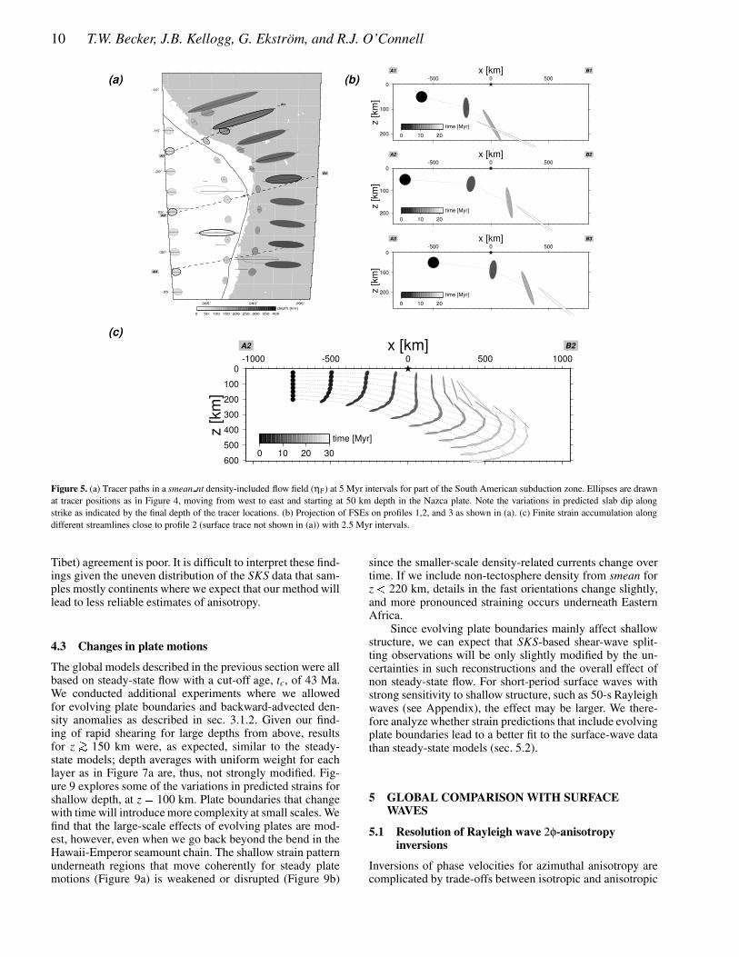
For the strain evolution example at convergent margins(Figure 5), we include ngrand nt density in the flow calcula-tion. The strain development can be divided into two stages:first, we see compression in the plane of the slab as materialenters the mantle. The largest stretching axes are nearly ra-dial, and the horizontal part of the FSE shows trench-parallelelongation. In the second stage, for greater depths and partic-ularly owing to the inclusion of slab pull forces, deep stretch-ing becomes more important and leads to deformations suchthat the largest stretching axes rotate mostly perpendicularto the trench and become more horizontal (Figure 5c).
Where the largest eigenvector points in a nearly ra-dial direction, the elongated horizontal part of the FSE ap-proximately follows the trench geometry and shows vary-ing degrees of trench-parallel alignment. In regions wheremeasurements for SKS waves, traveling nearly radially,yield zero or small anisotropy but where more horizontallypropagating local S phases show splitting (Fouch & Fis-cher 1998), this small horizontal deformation componentmay be important. This is particularly the case if crystallo-graphic fast axes are distributed in a ring rather than tightlyclustered around the largest FSE eigendirection, in whichcase the resolved anisotropy may be trench parallel. How-ever, Hall et al. (2000) show that synthetic splitting is mostlytrench-perpendicular in the back-arc region for simple flowgeometries, if fast wave propagation is assumed to be alwaysoriented with the largest FSE axis. Escape flow around a slabthat impedes large-scale currents in the mantle is thereforeusually invoked as an explanation for trench-parallel split-ting (e.g. Russo & Silver 1994; Buttles & Olson 1998).Yet, at least for some regions, 3-D circulation that is notdue to slab impediment might be invoked alternatively (Hallet al. 2000; Becker 2002).
4 GLOBAL FINITE-STRAIN MAPS
4.1 Plate-scale circulation
Figure 6a shows the global, τ � 10 Myr time interval, depth-averaged strain field for a circulation calculation that incor-
porates only plate-related flow using ηF. For simplicity, platemotions are assumed to be constant in time for 43 Myr. Wefocus on the horizontal projection of the largest stretchingdirection of L, showing the orientation of the FSE axis assticks whose lengths scale with ζ. The background shad-ing in Figure 6 shows ∆Lrr � Lrr � 1 as an indication ofstretching in the radial, r, direction. Strain was calculatedfor � 10 000 approximately evenly distributed tracers ( � 2
�spacing at equator) for each layer, which were placed from50 km through 400 km depth at 50 km intervals to sample theupper mantle above the 410-km phase transition. The hori-zontal projections of the largest axes of the FSE are depth av-eraged after weighting them with the ζ-scaled strain at eachlocation (sec. 3.3), while the radial, ∆Lrr, part is obtainedfrom a simple depth average. The horizontal strain orienta-tions will be interpreted as a measure of the depth-averagedazimuthal anisotropy as imaged by Rayleigh waves.
The finite-strain field of Figure 6a is similar to instanta-neous strain-rates in terms of the orientations of largest ex-tension, which are dominated by the shearing of the uppermantle due to plate motions. However, orientations are notidentical to those expected to be produced directly from thesurface velocities because of 3-D flow effects. The depth-averaged strain for τ � 10 Myr is furthermore dominated byradial extension (positive ∆Lrr) at both ridges and trenches,unlike for instantaneous strain (or small τ) where ridges areunder average radial compression. This effect is due to theradial stretching of material that rises underneath the ridgesbefore being pulled apart sideways and radially compressedat the surface. This effect has been invoked in qualitativemodels of radial anisotropy (e.g. Karato 1998) and may ex-plain the fast vSV (vSV $ vSH at � 200 km depths) anomaly insurface wave models for the EPR (Boschi & Ekstrom 2002).Not surprisingly, strain accumulation for constant τ modelsis strongest underneath the fast-moving oceanic plates.
Figure 6b shows results for constant strain, ζc � 0 � 5, as-suming that this is a relevant reworking strain after whichall previous fabric is erased (Ribe 1992). As a conse-quence, most horizontal strains are of comparable strength,with some exceptions, such as the Antarctic plate around30�
W/60�
S. There, shearing is sufficiently slow that itwould take more than our cutoff value of 43 Ma to accu-mulate the ζc strain.
4.2 Mantle density driven flow
Figure 7 shows ζc � 0 � 5 depth-averaged strain for flow thatincludes the effect of plate-related motion plus internal den-sities as derived from tomography model smean (Table 1).With the caveat that we are interpreting the instantaneousflow that should be characteristic of mantle convection at thepresent day as steady state for several tens of Myr, we findthat the inclusion of mantle density leads to a concentrationof radial flow and deformation underneath South Americaand parts of East Asia. These features are related to sub-duction where the circum-Pacific downwellings exert strongforces on the overlying plates (cf. Steinberger et al. 2001;Becker & O’Connell 2001b). For ηF (Figure 7a), smaller-scale structure owing to density anomalies is most clearlyvisible within continental plates, which were characterizedby large-scale trends for plate motions alone. Other patternsinclude a west-east extensional orientation in East Africa,

Seismic anisotropy and mantle flow 9
(c)
(b)(a)
230˚ 235˚ 240˚ 245˚ 250˚ 255˚ 260˚ 265˚
-30˚
-25˚
-20˚
-15˚
-10˚
-5˚
0˚
A1 B1
A2
B2
A3
B3
0 50 100 150 200 250 300 350 400
depth [km]
0
100
200
300
z [k
m]
-1500 -1000 -500 0 500 1000 1500x [km]
0 10 20 30
time [Myr]
A2 B2
0
100
200
300
z [k
m]
-1500 -1000 -500 0 500 1000 1500x [km]
0 10 20
time [Myr]
A2 B2
0
100
200
300
z [k
m]
-1500 -1000 -500 0 500 1000 1500x [km]
0 10 20
time [Myr]
A1 B1
0
100
200
300
z [k
m]
-1500 -1000 -500 0 500 1000 1500x [km]
0 10 20
time [Myr]
A3 B3
Figure 4. (a) Projection of the largest principal axes of strain ellipsoids (sticks) and horizontal cut through FSEs (ellipses), shown centered at tracer positionsin purely plate-motion driven flow (ηF) around the East Pacific Rise. Tracer positions are shown at 5 Myr intervals, starting at 300 km depth, with depthgrayscale-coded. (b) Projection of FSEs for profiles 1, 2, and 3 as indicated by dashed lines in (a), ellipse shading corresponds to time. (c) Time evolution ofstrain for an expanded set of tracers along profile 2 (surface projection not shown in (a)) with 2.5 Myr time intervals.
related to an upwelling that correlates with the rift-zone tec-tonics. The predicted strain for ηG (Figure 7b) is, expectedly,more complex. Since the low viscosity notch of ηG partlydecouples the upper and lower mantle in terms of shearing,upwellings such as the one in the southwestern Pacific (thesuperswell region) are able to cause a stronger anisotropysignal than for the ηF model.
In contrast to the plate-motion only models, finite strainfrom density-driven flow is quite sensitive to the input mod-els and viscosity structures in terms of the local orienta-tions of the largest stretching axes. This is to be expected,given that tracer advection will amplify small differences be-tween tomographic models. Figure 7 is therefore only an il-lustration of the large-scale features predicted by the lowest-common-denominator tomography model smean; individualhigh resolution models (e.g. ngrand) lead to more irregularstrain predictions, but not to better model fits (sec. 5.2).
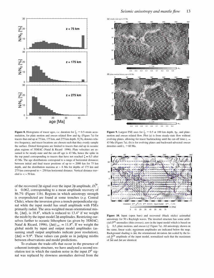
Figures 8 shows histograms for the time required toachieve ζc � 0 � 5 (“age”) for different depths based on themodel shown in Figure 7a. We find that many of the shallowstrain markers (within the high-viscosity lithospheric layer)have our age-limit of tc � 43 Ma, implying that strain accu-mulation is slow within the “plates” that move coherentlywithout large interior velocity gradients. For deeper lay-
ers, where shearing is stronger, strain is accumulated morerapidly such that ζ � 0 � 5 is reached by most tracers before20 Myr and at smaller horizontal advection distances thanat shallow depth. Most regions of slow strain accumulationare underneath continents where minima in the amplitudesof surface velocities are found. In general, however, ζ � 0 � 5strains are accumulated in a few Myr and small advectiondistances � O � 500 km / for all but the shallowest depths.
The depth average of Figure 7 hides variations of theorientation of the largest strain with depth. The rotation ofthe horizontal projection of the largest FSE axis between400 km depth and the surface can be in excess of 180
�(Becker 2002). Such complexity in strain is strong in, butnot limited to, regions of predominantly radial flow (cf.Figure 5). This finding may complicate the interpretationof anisotropy measurements, especially shear-wave splitting(Saltzer et al. 2000; Schulte-Pelkum & Blackman 2002).However, comparisons of our global horizontal projectionsof the largest principal axes of the FSE with observed split-ting orientations indicate agreement between strain and split-ting in (sparsely sampled) oceanic and in young continentalregions, e.g. the western US (Becker 2002). In older conti-nental regions (e.g. the eastern US and eastern South Amer-ica) and shear-dominated regions (e.g. New Zealand and NE
10 T.W. Becker, J.B. Kellogg, G. Ekstrom, and R.J. O’Connell
(c)
(b)(a)
0
100
200
300
400
500
600
z [k
m]
-1000 -500 0 500 1000x [km]
0 10 20 30
time [Myr]
A2 B2
0
100
200
z [k
m]
-500 0 500x [km]
0 10 20
time [Myr]
A1 B1
0
100
200z [k
m]
-500 0 500x [km]
0 10 20
time [Myr]
A3 B3
0
100
200
z [k
m]
-500 0 500x [km]
0 10 20
time [Myr]
A2 B2
285˚ 290˚ 295˚
-35˚
-30˚
-25˚
-20˚
-15˚
-10˚
A1
B1
A2
B2
A3
B3
0 50 100 150 200 250 300 350 400
depth [km]
Figure 5. (a) Tracer paths in a smean nt density-included flow field (ηF) at 5 Myr intervals for part of the South American subduction zone. Ellipses are drawnat tracer positions as in Figure 4, moving from west to east and starting at 50 km depth in the Nazca plate. Note the variations in predicted slab dip alongstrike as indicated by the final depth of the tracer locations. (b) Projection of FSEs on profiles 1,2, and 3 as shown in (a). (c) Finite strain accumulation alongdifferent streamlines close to profile 2 (surface trace not shown in (a)) with 2.5 Myr intervals.
Tibet) agreement is poor. It is difficult to interpret these find-ings given the uneven distribution of the SKS data that sam-ples mostly continents where we expect that our method willlead to less reliable estimates of anisotropy.
4.3 Changes in plate motions
The global models described in the previous section were allbased on steady-state flow with a cut-off age, tc, of 43 Ma.We conducted additional experiments where we allowedfor evolving plate boundaries and backward-advected den-sity anomalies as described in sec. 3.1.2. Given our find-ing of rapid shearing for large depths from above, resultsfor z $� 150 km were, as expected, similar to the steady-state models; depth averages with uniform weight for eachlayer as in Figure 7a are, thus, not strongly modified. Fig-ure 9 explores some of the variations in predicted strains forshallow depth, at z � 100 km. Plate boundaries that changewith time will introduce more complexity at small scales. Wefind that the large-scale effects of evolving plates are mod-est, however, even when we go back beyond the bend in theHawaii-Emperor seamount chain. The shallow strain patternunderneath regions that move coherently for steady platemotions (Figure 9a) is weakened or disrupted (Figure 9b)
since the smaller-scale density-related currents change overtime. If we include non-tectosphere density from smean forz 0 220 km, details in the fast orientations change slightly,and more pronounced straining occurs underneath EasternAfrica.
Since evolving plate boundaries mainly affect shallowstructure, we can expect that SKS-based shear-wave split-ting observations will be only slightly modified by the un-certainties in such reconstructions and the overall effect ofnon steady-state flow. For short-period surface waves withstrong sensitivity to shallow structure, such as 50-s Rayleighwaves (see Appendix), the effect may be larger. We there-fore analyze whether strain predictions that include evolvingplate boundaries lead to a better fit to the surface-wave datathan steady-state models (sec. 5.2).
5 GLOBAL COMPARISON WITH SURFACEWAVES
5.1 Resolution of Rayleigh wave 2φ-anisotropyinversions
Inversions of phase velocities for azimuthal anisotropy arecomplicated by trade-offs between isotropic and anisotropic

Seismic anisotropy and mantle flow 11
(a) τ 1 10 Myr0˚ 60˚ 120˚ 180˚ 240˚ 300˚ 360˚
-60˚
-30˚
0˚
30˚
60˚
-0.5 0.0 0.5
∆Lrr
ζ = 0.93
(b) ζc 1 0 2 50˚ 60˚ 120˚ 180˚ 240˚ 300˚ 360˚
-60˚
-30˚
0˚
30˚
60˚
-0.3 -0.2 -0.1 -0.0 0.1 0.2 0.3
∆Lrr
ζ = 0.46
Figure 6. Depth-averaged (upper mantle, 50 km � z � 400 km) finite strain for τ � 10 Myr (a) and ζc � 0 3 5 (b) strain accumulation. We use plate-motion relatedflow only and viscosity profile ηF. Thick sticks are plotted centered at every � 5th tracer location and indicate the orientation of the horizontal projection of thelargest axis of the FSE, scaled with the logarithmic strain ζ (see legend). Background shading denotes ∆Lrr � Lrr 4 1, and thin sticks denote the orientation ofsurface plate motions from NUVEL1-NNR. Colorscale for ∆Lrr is clipped at 70% of the maximum absolute value.
structure (e.g. Laske & Masters 1998) and the uneven ray-path coverage might map itself into apparent anisotropicstructure (e.g. Tanimoto & Anderson 1985). To ad-dress these issues, we performed recovery tests, shown forRayleigh waves at T � 50 s in Figure 10. The same inversionprocedure that was used to obtain the phase-velocity mapsshown in Figure 1 was employed to test our ability to recovera synthetic input model using the available data coverage.To make structure in the input model as realistic as possible,
2φ-anisotropy was inferred from the steady-state circulationmodel using smean, ηF, and ζc � 0 � 5 (cf. Figure 7a). Thehorizontal projections of the largest FSE axes were scaledwith ζ to roughly account for the strength of inferred seis-mic anisotropy; we additionally weighted each layer ac-cording to the 50-s Rayleigh wave sensitivity-kernel of Fig-ure A1. Maximum predicted strains were scaled to a 1.5%2φ-anisotropy amplitude (resulting in 0.6% RMS variation)and the isotropic and D4φ variations were set to zero. Ran-

12 T.W. Becker, J.B. Kellogg, G. Ekstrom, and R.J. O’Connell
(a) ηF
0˚ 60˚ 120˚ 180˚ 240˚ 300˚ 360˚
-60˚
-30˚
0˚
30˚
60˚
-0.3 -0.2 -0.1 -0.0 0.1 0.2 0.3
∆Lrr
ζ = 0.46
(b) ηG
0˚ 60˚ 120˚ 180˚ 240˚ 300˚ 360˚
-60˚
-30˚
0˚
30˚
60˚
-0.3 -0.2 -0.1 -0.0 0.1 0.2 0.3
∆Lrr
ζ = 0.47
Figure 7. Depth-averaged finite-strain for ζc � 0 3 5 strain accumulation in plate-motion and smean-driven flow for viscosity profiles ηF (a, cf. Figure 6b) andηG (b). Thin sticks in background are NNR plate velocities as in Figure 6.
dom noise was added to mimic the observational uncertain-ties. The resulting variance reduction of the inversion wasonly 14% for D0, implying that little of the spurious signalwas fit. Figure 10 shows that the orientations of azimuthalanisotropy of the input model are generally well recovered.Exceptions are found in the Middle East, in the Aleutians,the Cocos-Nazca plate area, and along the northern mid-Atlantic ridge system. To quantify these azimuthal devia-tions, we calculate the angular misfit ∆α (0
�65∆α
590�),
shown in a histogram in Figure 11a. We also compute 7∆α by
multiplying ∆α with the input model amplitudes to give lessweight to small-signal regions; 7∆α is shown as backgroundshading in Figure 10 and normalized such that weighted andoriginal maximum deviations are identical.
The amplitude recovery of the test inversion is not asgood as the azimuthal one. As shown in Figure 2, recoveryis worse on average in continental regions than in oceanicones; there, regions of poor recovery are found in the south-west Indian Ocean, the northern Atlantic, the Scotia plateregion, and the north-west Pacific. The average of the log10
Seismic anisotropy and mantle flow 13
0
10
20
30
N/N
0 [%
]
0 10 20 30 40
age [Ma]
z = 275 km
0
10
20
30
N/N
0 [%
]
z = 175 km
0
10
20
30N
/N0
[%]
z = 75 km
Figure 8. Histograms of tracer ages, i.e. duration for ζc � 0 3 5-strain accu-mulation, for plate motion and smean related flow and ηF (Figure 7a) fortracers that end up at 75 km, 175 km, and 275 km depth. N � N0 denotes rela-tive frequency, and tracer locations are chosen such that they evenly samplethe surface. Dotted histograms are limited to tracers that end up in oceanicplate regions of 3SMAC (Nataf & Ricard 1996). Plate velocities are as-sumed to be steady-state and the cut-off age is 43 Ma, hence the spike inthe top panel corresponding to tracers that have not reached ζ � 0 3 5 after43 Ma. The age distributions correspond to a range of horizontal distancesbetween initial and final tracer positions of up to � 2000 km for 75 kmdepth, and the distribution maxima at � 6 Ma for depths of 175 km and275 km correspond to � 250 km horizontal distance. Vertical distance trav-eled is 89� 50 km.
of the recovered 2φ signal over the input 2φ amplitude, D2φr ,
is � 0 � 062, corresponding to a mean amplitude recovery of86.7% (Figure 11b). Regions in which anisotropy strengthis overpredicted are found at some trenches (e.g. CentralChile), where the inversion gives a trench-perpendicular sig-nal while the input model has small amplitude with FSEsprimarily radial. The area-weighted mean orientational mis-fit, : ∆α ; , is 18.8
�, which is reduced to 13 � 4 � if we weight
the misfit by the input-model 2φ amplitudes. Restricting our-selves further to oceanic lithosphere (as given by 3SMAC;Nataf & Ricard, 1996), : ∆α ;<� oc = � 11 � 8 � . If we weight theglobal misfit by input and output model amplitudes (as-suming small output amplitudes indicate poor resolution),: ∆α ;>� 9 � 9 � . These values can guide us in judging misfitsbetween observations and model predictions.
To evaluate the trade-offs that occur in the presence ofcoherent isotropic structure, we have analyzed a second res-olution test in which the random noise in the input D0 sig-nal was replaced by slowness anomalies derived from the
(a) steady-state up to 43 Ma
0˚ 60˚ 120˚ 180˚ 240˚ 300˚ 360˚
-60˚
-30˚
0˚
30˚
60˚
-0.4 -0.3 -0.2 -0.1 0.0 0.1 0.2 0.3 0.4
∆Lrr
ζ = 0.50
(b) plate-motion history up to 60 Ma
0˚ 60˚ 120˚ 180˚ 240˚ 300˚ 360˚
-60˚
-30˚
0˚
30˚
60˚
-0.4 -0.3 -0.2 -0.1 0.0 0.1 0.2 0.3 0.4
∆Lrr
ζ = 0.50
Figure 9. Largest FSE axes for ζc � 0 3 5 at 100 km depth, ηF, and plate-motion and smean related flow. Plot (a) is from steady-state flow withoutevolving plates, allowing for tracer backtracking until the cut-off time tc �43 Ma (Figure 7a), (b) is for evolving plates and backward-advected smeandensities until tc � 60 Ma.
0˚ 60˚ 120˚ 180˚ 240˚ 300˚ 360˚
-60˚
-30˚
0˚
30˚
60˚
D4φ: 0.8%D2φ: 1.5%inversion: D2φ: 1.5%input model:
0 10 20 30 40 50 60 70∆α [deg]
Figure 10. Input (open bars) and recovered (black sticks) azimuthalanisotropy for 50 s Rayleigh waves. The inverted structure has some artifi-cial D4φ-anomalies (thin crosses), zero in the input model which is based onζc � 0 3 5, plate motions, and smean (cf. Figure 7a). All anisotropy shown onthe same, linear scale; maximum amplitudes are indicated below the map.Background shading is ?∆α, the orientational deviation ∆α scaled by the lo-cal D2φ amplitude of the input model, normalized such that the maximumof ?∆α and ∆α are identical.

14 T.W. Becker, J.B. Kellogg, G. Ekstrom, and R.J. O’Connell
(a)
0
10
20
N/N
0 [%
]
0 10 20 30 40 50 60 70 80 90
∆α [deg]
(b)
0
10
20
30
N/N
0 [%
]
-1 0 1
log10(D2φout/D2φ
in)
Figure 11. (a) Orientational misfit histogram ∆α (gray bars) for equal-areaspatial sampling of the recovery test of Figure 10, N � N0 denotes relativefrequency. Open bars show misfit when restricted to regions with input D2φ-amplitudes @ 25% of the maximum input. Dashed horizontal line denotesthe expected random distribution of misfit. (b) Histogram of amplitude re-covery, D2φ
r , as expressed by the decadic logarithm of inversion D2φ overinput D2φ-amplitudes (gray bars, open bars restricted to strong-amplitudeinput as in (a)).
crustal model CRUST5.1 (Mooney et al. 1998). The recov-ered anisotropic signal is similar to that of the first experi-ment, with mean azimuthal misfit : ∆α ;>� 13 � 7 � (weightedby input D2φ) and mean amplitude recovery of 87.1% forD2φ. If the 4φ-terms are suppressed by damping them muchmore strongly than D2φ, the result is, again, similar to thatshown in Figure 10, but the azimuthal misfit and amplituderecovery are slightly improved to : ∆α ;A� 12 � 5 � (weightedby input D2φ) and 90.3%, respectively. Assuming that theT � 50 s results are representative of deeper-sensing waves,the resolution tests are encouraging since they imply that Ek-strom’s (2001) inversions for azimuthal anisotropy are ro-bust. The number of parameters of an inversion for D2φ islarger than that of an isotropic inversion and the correspond-ing increase in degrees of freedom cannot be justified basedon the improvement in variance reduction alone (Laske &Masters 1998). However, the pattern that such an anisotropicinversion predicts is likely to be a real feature of the Earthand not an artifact.
5.2 Global azimuthal-anisotropy model fit
Figure 12 compares maps for Rayleigh wave 2φ anisotropyfrom Ekstrom’s (2001) inversions (Figure 1) with predic-tions from our preferred geodynamic model, obtained bydepth averaging (using the appropriate kernels) of the ζ-
0
10
20
N/N
0 [%
]
0 10 20 30 40 50 60 70 80 90
∆α [deg]
Figure 13. Histogram of orientational misfit, ∆α, between T � 50 sRayleigh wave 2φ anisotropy and model prediction for ζc � 0 3 5 strain, ηF,evolving plates (tc � 60 Ma), and smean nt advected density as in Fig-ure 12a. Solid bars: all data; open bars: data restricted to regions whereD2φ of the inversion is @ 0 3 25 times its maximum; and open bars with dot-ted lines: further restricted to oceanic lithosphere. Dashed horizontal lineindicates the expected random distribution of ∆α.
scaled horizontal projection of the largest axes of the FSE.The calculation uses ζc � 0 � 5-strain and includes the effectsof evolving plate motions, smean nt buoyancy, and changesin plate-configurations for tc � 60 Ma. We find that much ofthe measured signal in the oceans can be explained by LPOorientations and finite strain as predicted from our global cir-culation model. We show a histogram of the angular misfitfor T � 50 s in Figure 13; the largest misfits are typicallyfound in regions of small D2φ-amplitudes or in the conti-nents, where anisotropy may be related to past deformationepisodes.
The laterally averaged misfits are compared for severaldifferent models in Figure 14a and b for T � 50 s and T �150 s, respectively. We tried weighting the misfit in a num-ber of ways but think that, in general, accounting for both theinversion’s and the model’s D2φ-amplitudes is most appro-priate in order to avoid having poorly sampled regions bias: ∆α ; . For consistency, we have also weighted the surfaceplate-velocity derived misfits (APM and NNR) by the model(i.e. plate-velocity) amplitudes. However, such velocity-weighted misfits are biased toward the oceanic plates, whichmove faster than continental ones, relative to ζc � 0 � 5-strainmodels, which show a more uniform anisotropy-amplitudeglobally (e.g. Figure 7).
We find that most circulation-based strain models out-perform the hypotheses of alignment with NNR or APMplate motions. This distinction in model quality supportsour modeling approach and indicates that further study offinite strain models could lead to a better understanding oflithospheric deformation and mantle flow. The average fitto Ekstrom’s (2001) anisotropy maps is better for shorter(T � 50 s in Figure 14a) than for longer periods (T � 150 sin Figure 14b). This could be due to differences in resolutionof the surface waves, or the dominance of the plate-relatedstrains at shallow depths, presumably the best-constrainedlarge-scale features. We also observe a wider range in : ∆α ;for different types of models at T � 50 s than at T � 150 s.This is expected, given that strains accumulate more rapidlyat depth, so that it is, for instance, less important whether

Seismic anisotropy and mantle flow 15
(a) T B 50 s (peak D2φ-sensitivity: C 70 km depth)0˚ 60˚ 120˚ 180˚ 240˚ 300˚ 360˚
-60˚
-30˚
0˚
30˚
60˚
D2φ: 2.5%inversion: D2φ: 2.2%model:
0
10
20
30
40
50
60
70
∆αinvn [deg]
(b) T B 150 s (peak D2φ-sensitivity: C 200 km depth)0˚ 60˚ 120˚ 180˚ 240˚ 300˚ 360˚
-60˚
-30˚
0˚
30˚
60˚
D2φ: 2.1%inversion: D2φ: 1.6%model:
0
10
20
30
40
50
60
70
∆αinvn [deg]
Figure 12. Comparison of Rayleigh wave 2φ-azimuthal anisotropy for T � 50 s (a) and T � 150 s (b), shown as black sticks (maximum D2φ values shown toscale below map) and model anisotropy for ζc � 0 3 5, evolving plates (tc � 60 Ma), ηF, and smean nt advected density, shown as open bars. We omit D4φ fromthe inversions and scale the predicted anisotropy such that the RMS D2φ are identical to those from the inversions. Background shading indicates azimuthalmisfit scaled by the inverted D2φ amplitude such that maximum ∆α remains constant.

16 T.W. Becker, J.B. Kellogg, G. Ekstrom, and R.J. O’Connell
(a) T D 50 s (b) T D 150 s
25 30 35 40 45 50
⟨∆α⟩ [deg]
ηG tc = 60 Ma ngrand_nt
nuvel
nuvel.nnr
ηG tc = 60 Ma smean
base model
tc = 120 Ma
tc = 60 Ma
tc = 60 Ma ngrand_nt
ηG smean
ngrand_nt
tc = 60 Ma stb00d
ηG
ηG tc = 120 Ma tc = 60 Ma
smean
stb00d
lrr98d
tc = 60 Ma smean_nt
smean_nt
tc = 60 Ma smean
area
⟨∆α⟩recovery
ocean
D2φinv
D2φinv D2φ
mod
D2φinv D2φ
mod oc.
30 35 40 45 50
⟨∆α⟩ [deg]
ηG tc = 60 Ma ngrand_nt
ηG tc = 60 Ma smean
ηG smean
tc = 60 Ma ngrand_nt
ngrand_nt
nuvel
nuvel.nnr
tc = 60 Ma stb00d
ηG
stb00d
tc = 120 Ma
tc = 60 Ma
base model
smean
lrr98d
ηG tc = 120 Ma tc = 60 Ma
tc = 60 Ma smean_nt
smean_nt
tc = 60 Ma smean
area
⟨∆α⟩recovery
ocean
D2φinv
D2φinv D2φ
mod
D2φinv D2φ
mod oc.
Figure 14. Mean orientational misfit between 2φ anisotropy of Rayleigh waves at T � 50 s (a, cf. Figures 12a and 13) and T � 150 s (b) for a selection ofcirculation-derived, ζc � 0 3 5 finite-strain models, and surface plate-velocity orientations. The y-axis indicates different flow models; all models based on platemotions and viscosity profile ηF unless indicated otherwise. Types of density models abbreviated as in Table 1. If no time interval is specified, velocities aresteady-state with a cut-off in backward advection time, tc, of 43 Ma; tc � 60 Ma or tc � 120 Ma implies backward advection using evolving plate-boundariesand possibly density sources until tc. nuvel and nuvel.nnr refer to the azimuthal misfit as calculated from surface plate-velocity orientations for hotspot (HS2,APM) or NNR reference frames, respectively. The misfits, E ∆α F , are obtained by area-weighted averaging over a grid interpolation of predicted and observedanisotropy (filled stars). We additionally weight models by the surface-wave recovery function ?∆α as shown in the background of Figure 12 (open stars, mostlyhidden by filled ones), restrict misfit to oceanic regions (open diamonds), weight by the inversion’s D2φ-amplitude (filled circles), the inversion’s and themodel’s D2φ-amplitudes (filled boxes), and the latter quantity furthermore restricted to oceanic plates (open boxes). (For APM and NNR velocities, weightingby the model amplitudes implies a strong bias toward the oceanic plates relative to ζc � 0 3 5-models.) If we randomize the 2φ orientations of our models, wefind a standard deviation of G 0 3 4 H indicating that E ∆α FI89� 43 H is significantly different from the random mean of 45 H at the 5σ-level.
flow is treated as steady-state or with evolving plate bound-aries. For ηF, models that include buoyancy-driven flow leadto : ∆α ; improvements of � 6
�compared to those with plate
motions only. Comparing different density models, smeantypically leads to better results than higher resolution to-mography (ngrand) or models that are based on slabs only(stb00d or lrr98d). Including shallow density variations un-derneath younger plate regions (non-tectosphere models,“nt”), slightly improves the model fit.
Globally weighted results typically show the same de-pendence on model type as those that include only theoceanic lithosphere, : ∆α ;<� oc = ; the latter misfits are, however,generally smaller than the global estimates by � 4
�. The best
models yield : ∆α ;J� oc = � 24�
for T � 50 s and : ∆α ;<� oc = � 28�
for T � 100 s and T � 150 s, to be compared with 45�
for
random alignment and � 35�
for alignment with plate ve-locities. Taking the resolution of the surface wave inversionas imaged by the 7∆α function in Figure 10 into account im-proves the misfit, but not significantly. Regional variationsin misfit might therefore be due to poor surface-wave reso-lution but, globally, ∆α is independent of the surface-waveresolution pattern.
There are a number of second-order observations thathave guided us in the choice of the preferred model shownin Figure 12. τ-limited (time limited) strain-accumulationmodels lead to results that are similar to those of ζ-models(strain limited) without weighting. Results from τ calcu-lations with D2φ model-amplitude weighted : ∆α ; are al-ways, as expected, better than ζ-models because of the ad-ditional bias that is introduced toward the oceans (where

Seismic anisotropy and mantle flow 17
all models are more similar to the inversions). We there-fore limit consideration to ζc-models, for which we find thatdensity-included flow calculations lead to better results forηF than for ηG ( � 2
�difference in average : ∆α ; ). For shal-
low (T � 50 s) structure where strain accumulation is rep-resentative of a longer timespan, : ∆α ; values are slightlyimproved (not shown) when we include a “freezing” mech-anism for strains at shallow depths where the temperaturein the lithosphere might be too low for continuous fabricreworking (Becker 2002) but this is, again, partly due tothe resulting bias toward the oceanic regions. We cannotfind any significant global improvement compared to contin-uous strain-accumulation models. Comparing models withsteady-state velocities or evolving plates in Figure 14 we do,however, see a small ( � 2
�) decrease in global misfit when
the last 60 Ma of plate reconfiguration and density advectionare taken into account.
In summary, we find that the strain produced byglobal mantle circulation is a valid explanation for the az-imuthal anisotropy mapped by surface waves, and that suchcirculation-produced strain explains the pattern of azimuthalanisotropy better than does the pattern of absolute plate mo-tions. Further exploration of regional and global model per-formance can guide us in our understanding of anisotropy inthe upper mantle. While some of the regions where our mod-els disagree with anisotropy observations might be due tolimitations in our method (such as the assumptions about therelationship between strain and imaged anisotropy, sec. 2),others might indicate real effects such as intraplate deforma-tion (e.g. in the Australian plate) for which we have not ac-counted so far. Short-period surface-waves with good shal-low sensitivity may be able to provide us with constraints onthe strain history for times longer than a few tens of Myr andwill allow us to evaluate the degree of mantle-lithospherecoupling in different tectonic settings.
6 CONCLUSIONS
Observations of seismic anisotropy in the upper mantle canbe explained by global circulation models under the assump-tion that fast orientations are aligned with the largest axis ofthe finite strain ellipsoid, as suggested by the theory of Ribe(1992). Our models are very simplified in that we are usinga linear viscosity for the flow calculations and assume thatanisotropy obeys a straightforward relationship with finite-strain. However, it is encouraging that mantle-flow derivedmodels lead to smaller misfits with azimuthal anisotropyfrom surface waves than models based on alignment withsurface velocities. A coupled model that uses the strain his-tory predicted from a, possibly more sophisticated, circula-tion model as input for fabric development algorithms suchas that of Kaminski & Ribe (2001) should be attempted next.In this way, we should be able to both evaluate the validity ofour model assumptions and the generality of theories aboutthe origin of seismic anisotropy and tectonic deformation inthe upper mantle.
ACKNOWLEDGMENTS
All figures were produced with the GMT software by Wes-sel & Smith (1991). Bernhard Steinberger provided the orig-inal version of the flow code used for the circulation cal-culation, which would not have been possible without nu-merous authors’ willingness to share inversion and modelresults. Discussions with Karen Fischer and Paul Silver fur-thered our understanding of the implications of shear-wavesplitting measurements.
REFERENCES
Agee, C. B., 1998. Phase transformations and seismicstructure in the upper mantle and transition zone, inUltrahigh-Pressure Mineralogy. Physics and Chemistry ofthe Earth’s Deep Interior, edited by R. J. Hemley, vol. 37of Reviews in Mineralogy, pp. 165–203, MineralogicalSociety of America, Washington DC.
Anderson, D. L. & Dziewonski, A. M., 1982. Upper mantleanisotropy: evidence from free oscillations, Geophys. J. R.astr. Soc., 69, 383–404.
Becker, T. W., 2002. Lithosphere–Mantle Interactions,Ph.D. thesis, Harvard University, Cambridge MA.
Becker, T. W. & Boschi, L., 2002. A comparison of tomo-graphic and geodynamic mantle models, Geochemistry,Geophysics, Geosystems, 3(2001GC000168).
Becker, T. W. & O’Connell, R. J., 2001. Predicting platevelocities with geodynamic models, Geochemistry, Geo-physics, Geosystems, 2(2001GC000171).
Becker, T. W. & O’Connell, R. J., 2001. Lithosphericstresses caused by mantle convection: The role of platerheology (abstract), EOS Trans. AGU, 82(47), T12C–0921.
Ben Ismail, W. & Mainprice, D., 1998. An olivine fabricdatabase; an overview of upper mantle fabrics and seismicanisotropy, Tectonophysics, 296, 145–157.
Blackman, D. K. & Kendall, J.-M., 2002. Seismicanisotropy of the upper mantle: 2. Predictions for currentplate boundary flow models, Geochemistry, Geophysics,Geosystems, 3(2001GC000247).
Blackman, D. K., Wenk, H.-R., & Kendall, J.-M., 2002.Seismic anisotropy of the upper mantle: 1. Factors that af-fect mineral texture and effective elastic properties, Geo-chemistry, Geophysics, Geosystems, 3(2001GC000248).
Boschi, L. & Ekstrom, G., 2002. New images of the Earth’supper mantle from measurements of surface-wave phasevelocity anomalies, J. Geophys. Res., in press.
Bunge, H.-P. & Grand, S. P., 2000. Mesozoic plate-motionhistory below the northeast Pacific Ocean from seismicimages of the subducted Farallon slab, Nature, 405, 337–340.
Bunge, H.-P., Richards, M. A., Lithgow-Bertelloni, C.,Baumgardner, J. R., Grand, S. P., & Romanowicz, B. A.,1998. Time scales and heterogeneous structure in geody-namic earth models, Science, 280, 91–95.
Bunge, H.-P., Hagelberg, C., & Travis, B., 2001. Mantlecirculation models with variational data assimilation: In-ferring past mantle flow and structure from plate motionhistories and seismic tomography (abstract), EOS Trans.AGU, 82(47), NG51C–07.

18 T.W. Becker, J.B. Kellogg, G. Ekstrom, and R.J. O’Connell
Buttles, J. & Olson, P., 1998. A laboratory model of sub-duction zone anisotropy, Earth Planet. Sci. Lett., 164,245–262.
Chastel, Y. B., Dawson, P. R., Wenk, H.-R., & Bennett,K., 1993. Anisotropic convection with implications for theupper mantle, J. Geophys. Res., 98, 17757–17771.
Christensen, U. R., 1984. Convection with pressure- andtemperature-dependent non-newtonian rheology, Geo-phys. J. R. astr. Soc., 77, 343–384.
Dahlen, F. A. & Tromp, J., 1998. Theoretical Global Seis-mology, Princeton University Press, Princeton, New Jer-sey.
DeMets, C., Gordon, R. G., Argus, D. F., & Stein, S., 1990.Current plate motions, Geophys. J. Int., 101, 425–478.
Ekstrom, G., 2001. Mapping azimuthal anisotropy ofintermediate-period surface waves (abstract), EOS Trans.AGU, 82(47), S51E–06.
Ekstrom, G. & Dziewonski, A. M., 1998. The uniqueanisotropy of the Pacific upper mantle, Nature, 394, 168–172.
Fornberg, B., 1996. A practical guide to pseudospectralmethods, Cambridge University Press, Cambridge UK.
Forsyth, D. W., 1975. The early structural evolution andanisotropy of the oceanic upper mantle, Geophys. J. R.astr. Soc., 43, 103–162.
Fouch, M. J. & Fischer, K. M., 1998. Shear waveanisotropy in the Mariana subduction zone, Geophys. Res.Lett., 25, 1221–1224.
Gordon, R. G. & Jurdy, D. M., 1986. Cenozoic global platemotions, J. Geophys. Res., 91, 12389–12406.
Gudmundsson, O. & Sambridge, M., 1998. A regionalizedupper mantle (RUM) seismic model, J. Geophys. Res.,103, 7121–7136.
Hager, B. H. & Clayton, R. W., 1989. Constraints on thestructure of mantle convection using seismic observations,flow models, and the geoid, in Mantle convection; platetectonics and global dynamics, edited by W. R. Peltier,vol. 4 of The Fluid Mechanics of Astrophysics andGeophysics, pp. 657–763, Gordon and Breach SciencePublishers, New York, NY.
Hager, B. H. & O’Connell, R. J., 1981. A simple globalmodel of plate dynamics and mantle convection, J. Geo-phys. Res., 86, 4843–4867.
Hall, C. E., Fischer, K. M., & Parmentier, E. M., 2000. Theinfluence of plate motions on three-dimensional back arcmantle flow and shear wave splitting, J. Geophys. Res.,105, 28009–28033.
Hess, H. H., 1964. Seismic anisotropy of the uppermostmantle under oceans, Nature, 203, 629–631.
Ji, S., Zhao, X., & Francis, D., 1994. Calibration of shear-wave splitting in the subcontinental upper mantle beneathactive orogenic belts using ultramafic xenoliths from theCanadian Cordillera and Alaska, Tectonophysics, 239, 1–27.
Jung, H. & Karato, S.-i., 2001. Water-induced fabric tran-sitions in olivine, Science, 293, 1460–1463.
Kaminski, E. & Ribe, N. M., 2001. A kinematic model forfor recrystallization and texture development in olivinepolycrystals, Earth Planet. Sci. Lett., 189, 253–267.
Kaminski, E. & Ribe, N. M., 2002. Time scales for the evo-lution of seismic anisotropy in mantle flow, Geochemistry,Geophysics, Geosystems, 3(2001GC000222).
Karato, S.-i., 1998. Seismic anisotropy in the deep man-tle, boundary layers and the geometry of convection, PureAppl. Geophys., 151, 565–587.
Laske, G. & Masters, G., 1998. Surface-wave polarizationdata and global anisotropic structure, Geophys. J. Int.,132, 508–520.
Lithgow-Bertelloni, C. & Richards, M. A., 1998. The dy-namics of Cenozoic and Mesozoic plate motions, Rev.Geophys., 36, 27–78.
Lithgow-Bertelloni, C. & Silver, P. G., 1998. Dynamic to-pography, plate driving forces and the African superswell,Nature, 395, 269–272.
Lithgow-Bertelloni, C., Richards, M. A., Ricard, Y.,O’Connell, R. J., & Engebretson, D. C., 1993. Toroidal-poloidal partitioning of plate motions since 120 Ma, Geo-phys. Res. Lett., 20, 375–378.
Love, A. E. H., 1927. A Treatise on the Mathematical The-ory of Elasticity, Cambridge University Press, Cambridge,Reprinted in 1944 by Dover Publications, New York.
Mainprice, D., Barruol, G., & Ben Ismail, W., 2000. Theseimic anisotropy of the Earth’s mantle: From singlecrystal to polycrystal, in Earth’s deep interior. Mineralphysics and tomography from the atomic to the globalscale, edited by S.-i. Karato, A. M. Forte, R. C. Lieber-mann, G. Masters, & L. Stixrude, vol. 117 of GeophysicalMonograph, pp. 237–264, American Geophysical Union,Washington DC.
McKenzie, D. & Jackson, J., 1983. The relationship be-tween strain rates, crustal thickening, paleomagnetism, fi-nite strain and fault movements within a deforming zone,Earth Planet. Sci. Lett., 65, 182–202.
McKenzie, D. P., 1979. Finite deformation during fluidflow, Geophys. J. R. astr. Soc., 58, 689–715.
Mitrovica, J. X. & Forte, A. M., 1997. Radial profile ofmantle viscosity: results from the joint inversion of con-vection and postglacial rebound observables, J. Geophys.Res., 102, 2751–2769.
Montagner, J.-P., 1994. What can seismology tell us aboutmantle convection?, Rev. Geophys,, 32, 115–137.
Montagner, J.-P., 1998. Where can seismic anisotropy bedetected in the Earth’s mantle? in boundary layers, PureAppl. Geophys., 151, 223–256.
Montagner, J.-P. & Guillot, L., 2000. Seismic anisotropyin the Earth’s mantle, in Problems in Geophysics forthe New Millenium, edited by E. Boschi, G. Ekstrom, &A. Morelli, pp. 217–253, Istituto Nazionale di Geofisica eVulcanologia, Editrice Compositori, Bologna, Italy.
Montagner, J.-P. & Nataf, H.-C., 1986. A simple methodfor inverting the azimuthal anisotropy of surface waves, J.Geophys. Res., 91, 511–520.
Montagner, J.-P. & Tanimoto, T., 1991. Global upper man-tle tomography of seismic velocities and anisotropies, J.Geophys. Res., 96, 20337–20351.
Montagner, J.-P., Griot-Pommera, D.-A., & Lavee, J., 2000.How to relate body wave and surface wave anisotropy?, J.Geophys. Res., 105, 19015–19027.
Mooney, W. D., Laske, G., & Masters, G., 1998. CRUST5.1: a global crustal model at 5 degrees
�5 degrees, J.
Geophys. Res., 103, 727–747.Nataf, H.-C. & Ricard, Y., 1996. 3SMAC: an a priori tomo-
graphic model of the upper mantle based on geophysicalmodeling, Phys. Earth Planet. Inter., 95, 101–122.

Seismic anisotropy and mantle flow 19
Nicolas, A. & Christensen, N. I., 1987. Formation ofanisotropy in upper mantle peridotites; a review, inComposition, structure and dynamics of the lithosphere-asthenosphere system, edited by K. Fuchs & C. Froide-vaux, vol. 16 of Geodynamics, pp. 111–123, AmericanGeophysical Union, Washington DC.
Nishimura, C. E. & Forsyth, D. W., 1989. The anisotropicstructure of the upper mantle in the Pacific, Geophys. J.,96, 203–229.
O’Connell, R. J., Gable, C. W., & Hager, B. H., 1991.Toroidal-poloidal partitioning of lithospheric plate mo-tions, in Glacial Isostasy, Sea-Level and Mantle Rheology,edited by R. Sabadini, pp. 535–551, Kluwer AcademicPublishers, Amsterdam.
Panasyuk, S. V. & Hager, B. H., 1998. A model of transfor-mational superplasticity of the upper mantle, Geophys. J.Int., 133, 741–755.
Peselnick, L. & Nicolas, A., 1978. Seismic anisotropy in anophiolite peridotite. Application to oceanic upper mantle,Geophys. Res. Lett., 83, 1227–1235.
Press, W. H., Teukolsky, S. A., Vetterling, W. T., & Flan-nery, B. P., 1993. Numerical Recipes in C: The Art ofScientific Computing, Cambridge University Press, Cam-bridge, 2nd edn.
Ranalli, G., 1995. Rheology of the Earth, Chapman & Hall,London, 2nd edn.
Ribe, N. M., 1989. Seismic anisotropy and mantle flow, J.Geophys. Res., 94, 4213–4223.
Ribe, N. M., 1992. On the relation between seismicanisotropy and finite strain, J. Geophys. Res., 97, 8737–8747.
Ricard, Y. & Vigny, C., 1989. Mantle dynamics with in-duced plate tectonics, J. Geophys. Res., 94, 17543–17559.
Ricard, Y., Doglioni, C., & Sabadini, R., 1991. Differentialrotation between lithosphere and mantle: A consequenceof lateral mantle viscosity variations, J. Geophys. Res., 96,8407–8415.
Romanowicz, B. & Snieder, R., 1988. A new formalismfor the effect of lateral heterogeneity on normal modesand surface waves. II. General anisotropic perturbation,Geophys. J., 93, 91–99.
Russo, R. M. & Silver, P. G., 1994. Trench-parallel flowbeneath the Nazca plate from seismic anisotropy, Science,263, 1105–1111.
Saltzer, R. L., Gaherty, J. B., & Jordan, T. H., 2000. Howare vertical shear wave splitting measurements affected byvariations in the orientation of azimuthal anisotropy withdepth?, Geophys. J. Int., 141, 374–390.
Savage, M. K., 1999. Seismic anisotropy and mantle defor-mation: What have we learned from shear wave splitting?,Rev. Geophys., 37, 65–106.
Schott, B., Yuen, D. A., & Schmeling, H., 2000. The signif-icance of shear heating in continental delamination, Phys.Earth Planet. Inter., 118, 273–290.
Schulte-Pelkum, V. & Blackman, D. K., 2002. A synthesisof seismic P and S anisotropy, Geophys. J. Int., submit-ted.
Schulte-Pelkum, V., Masters, G., & Shearer, P. M., 2001.Upper mantle anistropy from long-period P polarization,J. Geophys. Res., 106, 21917–21934.
Silver, P. G., 1996. Seismic anisotropy beneath the con-tinents: probing the depths of geology, Ann. Rev. Earth
Planet. Sci., 24, 385–432.Smith, M. L. & Dahlen, F. A., 1973. The azimuthal de-
pendence of Love and Rayleigh wave propagation in aslightly anisotropic medium, J. Geophys. Res., 78, 3321–3333.
Steinberger, B., 2000. Slabs in the lower mantle – results ofdynamic modelling compared with tomographic imagesand the geoid, Phys. Earth Planet. Inter., 118, 241–257.
Steinberger, B. & O’Connell, R. J., 1998. Advection ofplumes in mantle flow: implications for hotspot motion,mantle viscosity, and plume distribution, Geophys. J. Int.,132, 412–434.
Steinberger, B., Schmeling, H., & Marquart, G., 2001.Large-scale lithospheric stress field and topography in-duced by global mantle circulation, Earth Planet. Sci.Lett., 186, 75–91.
Tanimoto, T. & Anderson, D. L., 1985. Lateral heterogene-ity and azimuthal anisotropy of the upper mantle: Loveand Rayleigh waves 100–250 s, J. Geophys. Res., 90,1842–1858.
Tommasi, A., 1998. Forward modeling of the developmentof seismic anisotropy in the upper mantle, Earth Planet.Sci. Lett., 160, 1–13.
Tommasi, A., Mainprice, D., Canova, G., & Chastel, Y.,2000. Viscoplastic self-consistent and equilibrium-basedmodelling of olivine lattice preferred orientation. 1. Im-plications for the upper mantle seismic anisotropy, J. Geo-phys. Res., 105, 7893–7908.
van Keken, P. & Zhong, S., 1999. Mixing in a 3D spheri-cal model of present-day mantle convection, Earth Planet.Sci. Lett., 171, 533–547.
Vinnik, L. P., Farra, V., & Romanowicz, B., 1989. Az-imuthal anisotropy in the Earth from observations of SKSat Geoscope and Nars broadband stations, Bull. seism.Soc. Am., 79, 1542–1558.
Vinnik, L. P., Makeyeva, L. I., Milev, A., & Usenko, Y.,1992. Global patterns of azimuthal anisotropy and defor-mation in the continental mantle, Geophys. J. Int., 111,433–447.
Wenk, H.-R. & Tome, C. N., 1999. Modeling dynamic re-crystallization of olivine aggregates deformed in simpleshear, J. Geophys. Res., 104, 25513–25527.
Wenk, R., Bennett, K., Canova, G. R., & Molinari, A.,1991. Modelling plastic deformation of peridotite with theself-consistent theory, J. Geophys. Res., 96, 8337–8349.
Wessel, P. & Smith, W. H. F., 1991. Free software helpsmap and display data, EOS Trans. AGU, 72, 445–446.
Wolfe, C. J. & Solomon, S. C., 1998. Shear-wave splittingand implications for mantle flow beneath the MELT re-gion of the East Pacific rise, Science, 280, 1230–1232.
Zhang, S. & Karato, S.-I., 1995. Lattice preferred orienta-tion of olivine aggregates deformed in simple shear, Na-ture, 375, 774–777.
APPENDIX A: DEPTH SENSITIVITY OF SURFACEWAVES TO AZIMUTHAL ANISOTROPY
Our treatment closely follows that of Montagner & Nataf(1986) and Montagner & Tanimoto (1991). The eigenfunc-tions of high- � normal modes can be used to construct

20 T.W. Becker, J.B. Kellogg, G. Ekstrom, and R.J. O’Connell
Frechet derivatives (or sensitivity kernels), Km, that charac-terize the effect of small perturbations in a parameter m at acertain depth r on changing the phase velocity c of a surfacewave:
km � c r K� mKm � m∂c∂m� (A1)
Here, m stands for an elastic modulus or density ρ (e.g.Dahlen & Tromp 1998, p. 335ff). For a transverselyisotropic Earth model such as PREM, the elasticity tensoris reduced from its most general form with 21 independentcomponents to five constants, A, C, F , L, and N in the no-tation of Love (1927). We write the perturbations in c in atransversely isotropic medium as
dc �ML R
0 N dCC
kC� dA
AkA� dL
LkL� (A2)
dNN
kN� dF
FkF� dρ
ρkρ O �
For wave propagation in an elastic medium that has the mostgeneral form of anisotropy, Smith & Dahlen (1973) showedthat the azimuthal dependence of Love and Rayleigh wavespeed anomalies can be expanded as given in (1). Montagner& Nataf (1986) demonstrated that the sensitivity kernels forthe D-terms can be retrieved from the kernels already con-structed for transversely isotropic models as in (A2). Mon-tagner & Nataf also found that the 4φ terms should gener-ally be small for predominantly horizontal alignment of fastpropagation axes based on measurements of elasticity ten-sors from the field. Rayleigh waves are more sensitive tothe 2φ component than Love waves, and only the 2φ termis readily interpreted in terms of fast horizontal propagationaxes in a strained medium with lattice-preferred orientation.Following our expectations, the observed 4φ signal is smallerthan the 2φ signal in most regions, with aforementioned ex-ception in regions of radial flow (sec. 2).
We shall therefore focus on D2φ for Rayleigh waves.Montagner & Nataf (1986) find that sensitivity kernels forthe cos � 2φ and sin � 2φ terms can be written as
kRayleighcos P 2φ QSR sin P 2φ Q � BC R S
AkA� HC R S
FkF� GC R S
LkL � (A3)
The six fractions with BC R S, HC R S, and GC R S are simple func-tions of Ci j (Montagner & Nataf 1986, eq. 5) and determinethe relative weights of the kA R F R L kernels. While Montagner& Nataf’s (1986) analysis of the effect of anisotropy was re-stricted to a flat Earth, Romanowicz & Snieder (1988) wereable to recover Montagner & Nataf’s approximation asymp-totically for large � in a more complete treatment. Follow-ing Montagner & Tanimoto (1991), we can therefore ob-tain the depth sensitivity of Rayleigh waves to azimuthalanisotropy with (A3) if we use elastic moduli for some rep-resentative anisotropic material whose fast propagation axisis assumed to be in the horizontal plane. Table A1 lists therelevant parameters for an oceanic sample from Peselnick &Nicolas (1978) (as used by Montagner & Nataf 1986) andfor Nunuvak from Ji et al.’s (1994) data (as used by Sav-age 1999). The BC R S and GC R S ratios are consistently largerthan the HC R S ratio. Since the kL kernel is additionally some-what larger than kA and kF , the GC R S � LkL term is mostly re-sponsible for the depth sensitivity of Rayleigh waves to the
Table A1. Ratios of elastic coefficients for 2φ contributions as in (A3)for two different rock samples from the indicated sources. cos and sin de-note the C T S constants. Since the partitioning of these ratios depends on thehorizontal coordinate frame, we also give the amplitude U cos2 V sin2
norm,normalized by the maximum ratio in each row.
type BC W SA
HC W SF
GC W SL
Peselnick & Nicolas (1978)cos 0 3 034 0 3 003 0 3 028sin 4 0 3 002 0 3 006 4 0 3 008U cos2 V sin2
norm 1 3 0 0 3 176 0 3 853Nunuvak (Ji et al. 1994)
cos 0 3 075 0 3 014 0 3 054sin 4 0 3 009 4 0 3 004 4 0 3 009U cos2 V sin2
norm 1 3 0 0 3 197 0 3 724
0
100
200
300
400
500
600
700 0 0.2 0.4 0.6 0.8 1
dept
h [k
m]
normalized sensitivity [A.U.]
50 s (0S202)100 s (0S97)150 s (0S62)
Figure A1. D2φ sensitivity kernels for Rayleigh waves with periods of 50 s,100 s, and 150 s for anisotropic PREM, normalized to their respective max-imum value. Kernels are shown for the amplitude of all 2φ terms and arecalculated from (A3) and the data of Peselnick & Nicolas (1978) in Ta-ble A1.
2φ anisotropy, shown in Figure A1 for surface waves withperiods of T � 50 s, T � 100 s, and T � 150 s.
Phase-velocity sensitivity kernels were estimated basedon normal-mode eigenfunctions computed for radiallyanisotropic PREM with the MINEOS program by G. Masters(e.g. Dahlen & Tromp 1998, p. 335). For the elastic param-eters under consideration, the sensitivity of Rayleigh wavesto azimuthal anisotropy has a depth dependence that is verysimilar to their kVSV kernels. We use the 2φ kernels to averagethe horizontal projections of the inferred fast-propagationaxes from strain at each depth when we compare our model-ing results with surface-wave based anisotropy.