comparing three error criteria for selecting radial basis function network topology

Comput. Methods Appl. Mech. Engrg. 198 (2009) 2137–2150

Contents lists available at ScienceDirect

Comput. Methods Appl. Mech. Engrg.

journal homepage: www.elsevier .com/locate /cma

Comparing three error criteria for selecting radial basis functionnetwork topology

Tushar Goel *, Nielen StanderLivermore Software Technology Corporation, 7374 Las Positas Road, Livermore, CA 94551, United States

a r t i c l e i n f o a b s t r a c t

Article history:Received 20 August 2008Received in revised form 15 January 2009Accepted 7 February 2009Available online 20 February 2009

Keywords:Radial basis functions networkCross-validationCrashworthinessMetamodelsTopology selection criterion

0045-7825/$ - see front matter � 2009 Elsevier B.V. Adoi:10.1016/j.cma.2009.02.016

* Corresponding author. Tel.: +1 925 245 4547; faxE-mail address: [email protected] (T. Goel).

The performance of radial basis function networks largely depends on the choice of topology i.e., locationand number of centers, radius of influence, etc. Thus finding the best network is a multi-level optimiza-tion problem. It is obvious that different criteria for optimization would result in different network topol-ogies. A systematic study is carried out to compare the most widely used root mean square error criterionfor topology selection with cross-validation based methods like PRESS or PRESS-ratio. The main focushere is to find the best criterion to select RBF network topology. Based on a suite of analytical examplesand crashworthiness simulation problems, it was concluded that the PRESS-based selection criterion per-forms the best and offers the least variation with the choice of experimental design, sampling density,and the nature of the problem.

� 2009 Elsevier B.V. All rights reserved.

1. Introduction

Most engineering problems of practical significance are com-putationally expensive. This phenomenon is common in crash-worthiness optimization due to the high cost of the finiteelement simulations. To alleviate high computational cost, theuse of meta-models has become increasingly popular. In this ap-proach, meta-models are developed using the limited data andoptimization is carried out using these computationally inexpen-sive surrogate models. There are many types of meta-modelsavailable in literature with polynomial response surfaces beingthe most popular due to their simplicity. Radial basis functionnetworks (RBFs) have been gaining popularity for approximationbecause of their ability to model highly non-linear responseswith low fitting cost.

Numerous instances have been reported of the use of radialbasis functions in engineering applications. A small representa-tive sample of some engineering applications is given as follows.Kurdila and Peterson [1], Li et al. [2] and Young et al. [3] usedradial basis functions to approximate control conditions of non-linear systems applied to aircraft and rockets. Wheeler et al. [4]used radial basis functions to model high pressure oxidizer dis-charge temperature for a space shuttle main engine. Papilaet al. [5], Shyy et al. [6], Karakasis and Giannakoglou [7] used ra-dial basis functions to design turbo-machinery and propulsioncomponents. Meckesheimer et al. [8] used radial basis functions

ll rights reserved.

: +1 925 449 2507.

to approximate discrete/continuous responses in the design of adesk lamp. Rocha et al. [9] found RBFs to perform the best toapproximate wing weight of subsonic transport vehicle. Zhanget al. [10] used radial basis functions to optimize a microelec-tronic packaging system. Reddy and Ganguli [11] used radial ba-sis functions to assess structural damage in helicopter rotorblades. Glaz et al. [12] used RBFs to approximate vibration loadswhile designing the helicopter rotor blades. Panda et al. [13]used RBFs to predict flank wear in drills. Lanzi et al. [14] usedRBFs to approximate crash capabilities of composite absorbers.Fang et al. [15] found that RBFs approximate different responsesin crashworthiness simulations very well.

While numerous successful applications of RBFs are reported, itis important to note that the quality of an RBF approximation de-pends heavily on the topology of the network i.e., the number ofradial basis functions (neurons), location of centers of neurons,and radius of influence. Orr [16–20] and the references within dis-cusses different issues in the selection of the number and locationof centers and the radius of influence of neurons. To date, there isno consensus on the best method of selecting network topologythough it is agreed that network topology has a large bearing onthe output.

While generalized cross-validation error (also known as pre-dicted residual sum of squares or PRESS) has been demonstratedfor selecting neural network topology [21–25], a radial basis func-tion network typically minimizes the root mean square error crite-rion [16–20,26,27]. The influence of different criteria on theselection of RBF network topology is studied in this paper. Specif-ically, the most popular PRESS error criterion is compared with

mailto:[email protected]

http://www.sciencedirect.com/science/journal/00457825

http://www.elsevier.com/locate/cma

2138 T. Goel, N. Stander / Comput. Methods Appl. Mech. Engrg. 198 (2009) 2137–2150

other criteria like root mean square error, and integrated pointwiseratio of generalization error that is defined as PRESS-ratio in asubsequent Section. A few analytical test examples and engineer-ing application problems from crashworthiness simulations areused to compare the different methods.

The paper is arranged as follows. The theoretical model andstepwise procedure of the RBF model construction is described inthe next section. Performance metrics to appraise different criteriaand test problems used to validate the proposed approach are de-scribed in Section 3. The test procedure and numerical setup foreach example are detailed in Section 4. Results obtained for differ-ent examples are given in Section 5. Finally, the main conclusionsderived from this study are summarized in Section 6.

2. Radial basis function theoretical model

A response function f(x) is approximated using a metamodel ofthe response f ðxÞ as,

f ðxÞ ¼ f ðxÞ þ e; ð1Þ

where e is the error in approximation.

2.1. Regression problem

Radial basis functions (RBFs) were introduced as approximationfunctions by Hardy [28] in 1971 for approximation of topographi-cal data. This is a non-parametric approximation technique be-cause no global form of the approximation function is assumed apriori. Instead, the approximation f ðxÞ is represented as a linearcombination of NRBF radially symmetric functions (radial basisfunctions) h(x) as,

f ðxÞ ¼ w0 þXNRBF

i¼1

wihiðxÞ; ð2Þ

where wi is the weight associated with the ith radial basis function.While many monotonically radially varying functions have

been used as RBFs, the Gaussian function is the most commonlyused radial basis function. A typical Gaussian function h(x) at pointx is given as follows:

hðxÞ ¼ expð� x� ck k2=d2

c Þ ¼ expð�ðr=dcÞ2Þ; dc ¼ s� rc; ð3Þ

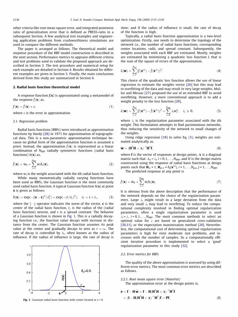
where the k � k operator indicates the norm of the vector, c is thecenter of the radial basis function, rc is the radius of the (radialbasis function) neuron, and s is a spread constant. The behaviorof a Gaussian function is shown in Fig. 1. This is a radially decay-ing function i.e., the function value decays with increase in dis-tance from the center. The Gaussian function assumes its peakvalue at the center and gradually decays to zero as r ?1. Therate of decay is controlled by dc, often known as the radius ofinfluence. If the radius of influence is large, the rate of decay is

Fig. 1. Gaussian radial basis function with center located at x = 0.

slow; and if the radius of influence is small, the rate of decayof the function is high.

Typically, a radial basis function approximation is a two-leveloptimization. Firstly, one needs to determine the topology of thenetwork i.e., the number of radial basis functions, correspondingcenter locations, radii, and spread constant. Subsequently, theweights associated with each RBF are estimated. Mostly, weightsare estimated by minimizing a quadratic loss function L that isthe sum of the square of errors of the approximation.

LðwÞ ¼XNpts

i¼1

ðf ðxðiÞÞ � f ðxðiÞÞÞ2: ð4Þ

This choice of the quadratic loss function allows the use of linearregression to estimate the weights vector [26] but this may leadto overfitting of the data and may result in very large weights. Mul-lur and Messac [27] proposed the use of an extended RBF to avoidoverfitting. However, a more conventional approach is to add aweight penalty to the loss function [29],

LðwÞ ¼XNpts

i¼1

ðf ðxðiÞÞ � f ðxðiÞÞÞ2 þXNRBF

i¼0

kiw2i ; ki P 0; ð5Þ

where ki is the regularization parameter associated with the ithweight. This formulation attempts to find parsimonious networks,thus reducing the sensitivity of the network to small changes ofthe weights.

Using ridge regression [18] to solve Eq. (5), weights are esti-mated analytically as,

w ¼ ðHT Hþ KÞ�1HT f; ð6Þ

where f is the vector of responses at design points, K is a diagonalmatrix such that Kii = ki, i = 0,1, . . . ,NRBF, and H is the design matrixconstructed using the response of radial basis functions at designpoints such that Hi1 = 1, Hij+1 = hj(x(i)), i = 1, . . . ,Npts, j = 1, . . . ,NRBF.

The predicted response at any point is

f ðxÞ ¼ w0 þXNRBF

i¼1

wihiðxÞ: ð7Þ

It is obvious from the above description that the performance ofthe network depends on the choice of the regularization param-eters. Large ki might result in a large deviation from the dataand very small ki may lead to overfitting. To reduce the compu-tational complexity involved in finding optimal regularizationparameters, often a single regularization parameter is usedki = k, i = 0,1, . . . ,NRBF. The most common methods to select anoptimal value for k are based on generalized cross-validation[30,31], or the expectation maximization method [20]. Neverthe-less, the computational cost of determining optimal regularizationparameters is high for even moderate size problems, and in-creases with the number of samples. So a computationally effi-cient iterative procedure is implemented to select a ‘good’regularization parameter in this study [32].

2.2. Error metrics for RBFs

The quality of the above approximation is assessed by using dif-ferent error metrics. The most common error metrics are describedas follows.

2.2.1. Root mean square error (NoiseVar)The approximation error at the design points is,

e ¼ f �H w_¼ f �HðHT Hþ KÞ�1HT f

¼ ðI�HðHT Hþ KÞ�1HTÞf ¼ Pf; ð8Þ

T. Goel, N. Stander / Comput. Methods Appl. Mech. Engrg. 198 (2009) 2137–2150 2139

where I is an identity matrix of size Npt and P = I � H(HTH + K)�1HT.P is known as the projection matrix. The root mean square error(also an estimate of square root of noise variance) [18] is,

r ¼ffiffiffiffiffiffiffiffiffiffiffiffiffiffiffiffiffiffiffiffiffiffiffiffiffiffiffiffiffiffiffiffiðeT eÞ=traceðPÞ

q: ð9Þ

2.2.2. Predicted residual sum of squares (PRESS)Leave-one-out cross-validation error or PRESS is another popu-

lar and effective error measure [33,34]. To compute PRESS, the re-sponse is approximated using the data at Npt � 1 points and thisapproximation is used to compute the actual error at the left outpoint. This procedure is repeated for all Npt points by leaving outeach point exactly once. The expression for PRESS is

PRESS ¼XNpts

i¼1

ðePRESSi Þ2 ¼

XNpts

i¼1

ðf ðxðiÞÞ � f�iðxðiÞÞÞ2; ð10Þ

where f�iðxðiÞÞ is the predicted response at design point x(i) whichwas not used to construct the approximation f�i. The need to fitmany networks to estimate PRESS can be obviated by using the pro-jection matrix [18] and the vector of leave-one-out cross-validationerror is computed as follows:

ePRESS ¼ ðdiagðPÞÞ�1Pf: ð11ÞThe root mean square of the PRESS which is compared to other errormeasures is

rPRESS ¼ffiffiffiffiffiffiffiffiffiffiffiffiffiffiffiffiffiffiffiffiffiffiffiffiPRESS=Npts

q: ð12Þ

2.2.3. Mean pointwise cross-validation error ratio (PRESS-ratio)While the leave-one-out cross-validation error is a good mea-

sure of actual error, it might be susceptible to the large magnitudeof individual error values. To avoid contamination of the predictionerror, a leave-one-out cross-validation error ratio based criterion isgiven as follows:

rratio ¼1

Npts

XNpts

i¼1

f ðxðiÞÞ � f�iðxðiÞÞf�iðxðiÞÞ

��: ð13Þ

This criterion scales the magnitude of the errors thus eliminatingthe influence of a few large errors on the predictions but assignsmore importance to the errors in the prediction of small values.

It is noted that additional cost is incurred to compute cross-val-idation error criteria (PRESS or PRESS-ratio). However, the cost isusually very small compared to the time required to acquire simu-lation response data.

2.3. RBF network topology selection

As discussed earlier, RBF network selection is a two-level opti-mization. The theoretical model for the second step, that is, theselection of weights for a given topology is well developed butthe optimal selection of network topology (first step) still requiressignificant effort. Consequently, a trial and error procedure is usedto select the suitable RBF network topology and optimal weightsare selected for the best topology.

A stepwise procedure to construct a radial basis function net-work that is adopted in LSOPT� [32] is given as follows.

1. Sample design points;2. Evaluate responses at design points;3. Select a criterion to select network topology;4. Select the number of neurons;

(a) Select a spread constant between 1.0 and 2.0;(i) Determine the location of centers and correspondingradii [32] of the neurons;

(ii) Estimate the best regularization parameter(s) usingan iterative scheme [32] with the chosen topology selec-tion criterion;(iii)Estimate the error measure according to the selectioncriterion;

(b) Repeat the loop over different spread constants;5. Select the best spread using the chosen topology selection

criterion;6. Repeat the loop (Step 4) for a different number of neurons;7. Select the network topology that results in the best perfor-

mance according to the chosen criterion.

There are three optimization steps in the selection of the RBFnetwork topology, (i) estimation of the regularization parameter,(ii) estimation of the spread constant, and (iii) choice of the num-ber of neurons. While the choice of selection criterion can be differ-ent at each step, a consistent choice is maintained here. A differentcriterion can be used as objective function of the optimization pro-cess, e.g., minimization of the root mean square error, PRESS error,or PRESS-ratio.

In this paper, a comparison of the above-mentioned three errorcriteria to select RBF network topology is carried out. To isolate theinfluence of the error criterion on the prediction performance, theorder in which a design point is selected as the center and corre-sponding radius of the neuron is fixed for the chosen experimentaldesign [32]. For the sake of simplicity, a single regularizationparameter is used for all weights ki = k "i.

3. Performance metrics and test problems

The performance of different RBF networks obtained by usingdifferent topology selection criteria is studied using a suite of ana-lytical and crashworthiness test problems on a few error metrics.The relevant error metrics and examples are given as follows.The performance metrics are based on independent test points.

3.1. Performance metrics

The performance of the predictions is compared using the fol-lowing four metrics.

3.1.1. Correlation between predicted and observed responsesThe correlation coefficient is calculated as

Rðf ; f Þ ¼ 1

V rðf Þrðf Þ� � Z

Vðf � �f Þðf � �

f ÞdV ; ð14Þ

where �f and r(f) are the mean and standard deviation of actual re-sponses, �

f and rðf Þ are the mean and standard deviation of the pre-dicted responses, and V is the volume of the domain. The mean andstandard deviations are computed as

�f ¼ 1V

ZV

fdV ; rðf Þ ¼

ffiffiffiffiffiffiffiffiffiffiffiffiffiffiffiffiffiffiffiffiffiffiffiffiffiffiffiffiffiffiffiffiffi1V

ZVðf � �f Þ2dV

s: ð15Þ

A high correlation coefficient is desired for a good quality ofapproximation.

The above equations are numerically evaluated using the dataat test points by implementing quadrature for the integration[42] as follows:

�f ¼XNtest

i¼1

cifi

,XNtest

i¼1

ci; rðf Þ ¼

ffiffiffiffiffiffiffiffiffiffiffiffiffiffiffiffiffiffiffiffiffiffiffiffiffiffiffiffiffiffiffiffiffiffiffiffiffiffiffiffiffiffiffiffiffiffiXNtest

i¼1

ciðfi � �f Þ2XNtest

i¼1

ci

,vuut ; ð16Þ

1V

ZV

f f dV ¼XNtest

i¼1

cifi f i

XNtest

i¼1

ci

,: ð17Þ


In the above equations, ci represents the weight associated with theith test point, as determined by the quadrature for integration. Foruniform grid of points, Simpson’s integration rule is used whereasfor non-uniform grids, the Monte Carlo integration method is used.

The correlation coefficient captures the prediction trends butyields no information about the actual errors of approximation,which can be high despite a high correlation. So the approximationerrors are quantified using two error-based criteria.

3.1.2. Root mean square error in the predictionsThe root mean square error at the test points is given as

RMSE ¼

ffiffiffiffiffiffiffiffiffiffiffiffiffiffiffiffiffiffiffiffiffiffiffiffiffiffiffiffiffiffiffiffiffi1V

ZVðf � f Þ2dV

s: ð18Þ

Using the quadrature, the RMSE is estimated as

RMSE ¼

ffiffiffiffiffiffiffiffiffiffiffiffiffiffiffiffiffiffiffiffiffiffiffiffiffiffiffiffiffiffiffiffiffiffiffiffiffiffiffiffiffiffiffiffiffiffiffiXNtest

i¼1

ciðfi � f iÞ2XNtest

i¼1

ci

,vuut : ð19Þ

3.1.3. Average relative error in the predictionsThe average relative error at the test points is given as

ARE ¼ 1V

ZV

f=f � 1� �

dV : ð20Þ

Using the quadrature, the average relative error is estimated as

ARE ¼XNtest

i¼1

ci fi=f i � 1� � XNtest

i¼1

ci

,: ð21Þ

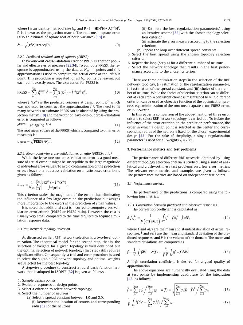
Table 1Parameters in the Hartman problem with three design variables.

i aij ci pij

1 3.0 10.0 30.0 1.0 0.3689 0.1170 0.26732 0.1 10.0 35.0 1.2 0.4699 0.4387 0.74703 3.0 10.0 30.0 3.0 0.1091 0.8732 0.55474 0.1 10.0 35.0 3.2 0.03815 0.5743 0.8828

Table 2Parameters in the Hartman problem with six design variables.

i aij ci

1 10.0 3.0 17.0 3.5 1.7 8.0 1.0

3.1.4. Maximum absolute error in the predictionsAnother measure of the quality of any approximation is the

maximum absolute error:

MaxE ¼maxi

fi � f i

�� : ð22Þ

A good approximation yields low errors and high correlation.

3.2. Test problems

Two types of test problems are used in this study,

1. Analytical examples2. Engineering problems from crashworthiness simulations

2 0.05 10.0 17.0 0.1 8.0 14.0 1.23 3.0 3.5 1.7 10.0 17.0 8.0 3.04 17.0 8.0 0.05 10.0 0.1 14.0 3.2

pij

1 0.1312 0.1696 0.5569 0.0124 0.8283 0.58862 0.2329 0.4135 0.8307 0.3736 0.1004 0.99913 0.2348 0.1451 0.3522 0.2883 0.3047 0.66504 0.4047 0.8828 0.8732 0.5743 0.1091 0.0381

3.2.1. Branin–Hoo function [35]

f ðx1; x2Þ ¼ �10þ 10 1� 18p

� �cosðx1Þ

þ x2 �5:14p2 x2

1 þ5:0p

x1 � 6� �

;

� 5 6 x1 6 10; 0 6 x2 6 15: ð23Þ

Table 3Parameters used in the JIN-10 function.

Value

t �6.089

3.2.2. Camelback function [35]

f ðx1; x2Þ ¼x4

1

3� 2:1x2

1 þ 4� �

x21 þ x1x2 þ 4x2

2 � 4�

x22;

� 3 6 x1 6 3; �2 6 x2 6 2: ð24Þ
1
t2 �17.164t3 �34.054t4 �5.914t5 �24.721t6 �14.986t7 �24.100t8 �10.708t9 �26.662t �22.179

3.2.3. Goldstein–Price [35]

f ðx1;x2Þ ¼ � 1þðx1þ x2þ1Þ2ð19�4x1þ3x21�14x2þ6x1x2þ3x2

2Þh i� 30þð2x1�3x2Þ2ð18�32x1þ12x2

1þ48x2�36x1x2þ27x22Þ

h i;

�26 x1 6 2; �26 x2 6 2: ð25Þ

3.2.4. Hartman [35]

f ðxÞ ¼ �X4

i¼1

ci exp �XNv

j¼1

aijðxj � pijÞ2

!; 0 6 xj 6 1; j ¼ 1;Nv :

ð26Þ

1. Three variables: Nv = 3, The parameters are given in Table 1.2. Six variables: Nv = 6, The parameters are given in Table 2. For

this example, all variables were allowed to vary between 0and 0.5.

3.2.5. Jin et al. [36] – two variables JIN2

f ðx1; x2Þ ¼ 30þ x1 sinðx1Þð Þ 4þ expð�x22Þ

� ;

0 6 x1 6 10; 0 6 x2 6 6: ð27Þ

3.2.6. Jin et al. [36] – 10 variables J10a

f ðxÞ ¼X10

j¼1

expðxjÞ tj þ xj � lnX10

i¼1

expðxiÞ ! !

;

0:5 6 xi 6 1; j ¼ 1;Nv : ð28Þ

The parameters used in this function are given in Table 3. This prob-lem is not really non-linear.

10

Fig. 2. Finite element models of a National Highway Transport and Safety Association vehicle.

Fig. 3. Exploded view of structural components in NHTSA vehicle influenced bydesign variables.

Table 4Design variables used for the multi-disciplinary crashworthiness simulation ofNational Highway Transport and Safety Association (NHTSA) vehicle.

Variable name Lower bound Baseline design Upper bound

Rail inner 1.0 2.0 3.0Rail outer 1.0 1.5 3.0Cradle rails 1.0 1.93 3.0Aprons 1.0 1.3 2.5Shotgun inner 1.0 1.3 2.5Shotgun outer 1.0 1.3 2.5Cradle cross member 1.0 1.93 3.0

Gauge

Radius

GaugeWidth

Width

DepthDepth

Depth

Width

Gauge Radius

Gauge

Radius

GaugeWidth

Width

DepthDepth

Depth

Width

Gauge Radius

Fig. 5. Design variables of the knee bolster system.

Fig. 4. Automotive instrument panel with knee bolster system used for knee-impact analysis (Courtesy: Ford Motor Company).


3.2.7. Giunta and Watson [37]

f ðxÞ ¼X10

j¼1

0:3þ sin1615

xj � 1� �

þ sin2 1615

xj � 1� ��

;

� 1 6 xi 6 1; j ¼ 1; Nv ; when Nv ¼ 5;0 6 xi 6 1; j ¼ 1; Nv ; when Nv ¼ 10: ð29Þ

This problem is studied for two instances of 5 and 10 variables.

3.2.8. Multi-disciplinary analysis of a NHTSA vehicle undergoing full-frontal crash

Next, a multi-objective optimization problem of the crashwor-thiness simulation of a National Highway Transportation andSafety Association (NHTSA) vehicle undergoing full-frontal impactwas analyzed. The goal of the optimization was to simultaneouslyreduce mass and intrusion, while satisfying the constraints on thetorsional frequency, maximum intrusion, and different stage pulses[38]. For this multi-disciplinary analysis, the finite element model,containing approximately 30,000 elements, was obtained from theNational Crash Analysis Center (NCAC website) [39]. A modal anal-ysis of the vehicle was conducted on the so-called ‘body-in-white’model with approximately 18,000 elements. The crash and vibra-tion finite element models are shown in Fig. 2 and the crash is sim-ulated for 90 ms.

The design variables were the gauges of different structuralmembers that were affected. These members included aprons, out-er and inner rails, inner and outer shotguns, cradle rail, and cradle

Table 5Design variables used for the simulation of automotive instrument panel structure(knee-impact) analysis.


L-Bracket gauge 0.7 1.1 3.0T-Flange depth 20.0 28.3 50.0


cross-members (Fig. 3). The description and ranges of these sevendesign variables is given in Table 4. The mathematical formulationof the optimization problem is as follows:

MinimizeMassIntrusion (xcrash)

F-Flange depth 20.0 27.5 50.0B-Flange depth 15.0 22.3 50.0I-Flange width 5.0 7.0 25.0L-Flange width 20.0 32.0 50.0R-Bracket gauge 0.7 1.1 3.0R-Flange width 20.0 32.0 50.0R-Bracket radius 10.0 15.0 25.0Bolster gauge 1.0 3.5 6.0Yolk radius 2.0 4.0 8.0

0 ms

Rib

TrimA-pillar

0 ms

Rib

TrimA-pillar

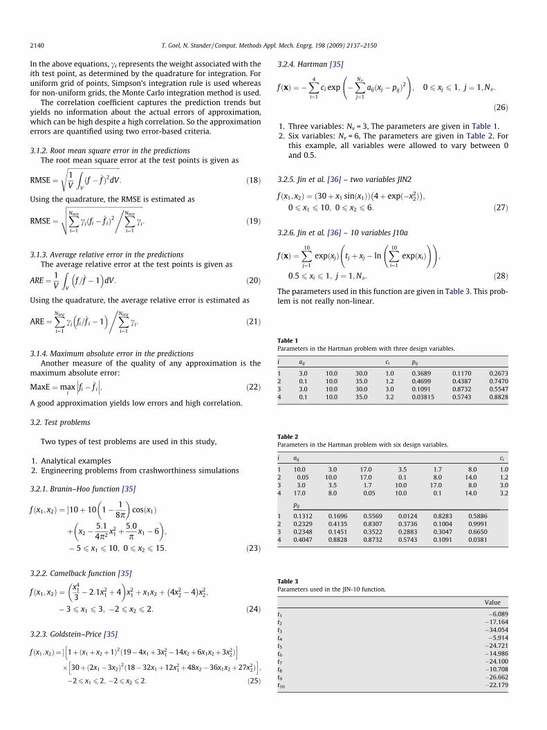
Fig. 6. Head impact of A-pillar with trim.

Table 6Design variables in head-impact analysis simulation.


Trim thickness 2.0 2.0 3.5Number of ribs 3 3 15Rib thickness 0.8 1.0 2.0Rib height 5.0 6.0 20.0Span 130.0 180 180

Subject to:Maximum intrusion <=551.27 mmStage 1 pulse (SP1) >=14.512 gStage 2 pulse (SP2) >=17.586 gStage 3 pulse (SP3) >=20.745 g41.385 Hz <=Torsional mode frequency <=42.38 Hz

The stage pulses are calculated from the SAE filtered (60 Hz)acceleration €x and displacement x of a left rear sill node as

Stage i pulse ¼ �kZ d2

d1

€xdxZ d2

d1

,dx

!; ð30Þ

where k = 0.5 for i = 1, otherwise k = 1. The minus sign was used toconvert acceleration to deceleration. The limits on the integrationfor different stage pulse were (0:184) for i = 1, (184:334) for i = 2,and (334: maximum displacement) for i = 3. LS-DYNA� [40] wasused to simulate different designs. It took approximately 50 minto run a single crashworthiness simulation on a dual-core IntelXeon (2.66 GHz) processor with 4 GB memory.

3.2.9. Automotive instrument panel structure (Knee-impact)simulation

The second crashworthiness example employs a finite elementsimulation of a typical automotive instrument panel (shown inFig. 4) impacting the knees [41]. The spherical object that repre-sents knee moves in the direction determined from prior physicaltests. The instrument panel (IP) comprises of a knee bolster thatalso serves as a steering column cover with a styled surface, andtwo energy absorption brackets attached to the cross vehicle IPstructure. A significant portion of the lower torso energy of theoccupant is absorbed by appropriate deformation of these brackets.The wrap-around of the knee around the steering column is de-layed by adding a device, known as the yoke, to the knee bolstersystem. The shape of the brackets and yoke are optimized withoutinterfering with the styled elements. The eleven design variablesare shown in Fig. 5 and the ranges are given in Table 5. To keepthe computational expense low, only the driver side instrumentpanel was modeled using 25,000 elements and the crash was sim-ulated for 40 ms, by which time the knees have been brought torest. The design optimization problem accounting for the optimaloccupant kinematics is formulated as follows:

MinimizeMass

Table 7Numerical setup for different examples. Nv is the number of variables, Npts is thenumber of samples used for approximation, NLHS is the number of basis points usedfor the D-optimality criterion, Npoly is the order of polynomial used for estimatingD-optimality, and Ntest is the number of test points.

Example Nv Npts NLHS Npoly Ntest

Branin–Hoo 2 20 100 3 150Camelback 2 30 150 4 150Goldstein–Price 2 42 200 5 150Jin-2 2 30 150 4 150Hartman-3 3 70 250 3 500GW5 5 100 400 3 2000Hartman-6 6 56 200 2 2000Jin-10a 10 150 450 2 5000GW10 10 150 450 2 5000NHTSAa 7 250 4847 – 4847Knee-impacta 11 100 851 – 851Head-impacta 5 42 1289 – 1289

a Experimental points are selected randomly from all the data points.

Subject to:Left knee force <=3250Right knee force <=3250Left knee displacement <=115Right knee displacement <=115Yoke displacement <=85Kinetic energy (KE) <=154,000

All responses are scaled. Knee forces are the peak SAE filtered(60 Hz) forces whereas all the displacements are represented bythe maximum intrusion. LS-DYNA [40] was used to simulate the dif-ferent designs. Each simulation requires approximately 60 minuteson a dual-core Intel Xeon (2.66 GHz) processor with 4 GB memory.

3.2.10. Head-impact analysisFinally, the impact of an occupant head form against an A-pillar

of a vehicle was analyzed. An interior trim cover with interior ribswas provided to soften the impact (Fig. 6). The design was required

Table 8Mean values of response at test points used to normalize errors.

Analytical NHTSA example Knee-impact example

BH 56 Mass 1.08 L-Force 1.35CB 20.3 Intrusion 522 R-Force 1.33GPR 3.64E+04 SP-1 15.5 L-Disp 0.841JIN2 128 SP-2 18.8 R-Disp 0.775HM3 1.79 SP-3 22.6 YokeDisp 0.651GW5 0.959 Freq 42.4 K.E. 0.39HM6 0.651 Head-impact example Mass 1.02GW10 1.27 HIC 584J10a 311 HIC_d 607


to minimize a head injury criterion (HIC-d) that was obtained fromthe head injury coefficient obtained at 15 ms (HIC). The designvariables for this example are given in Table 6. A single analysiswas completed in approximately 20 min on a dual-core Intel Xeon(2.66 GHz) processor with 4 GB memory.

4. Test procedure and numerical setup

4.1. Test procedure

For each test example, the stepwise test procedure to identifythe best topology selection criterion is outlined as follows:

1. Select an experimental design [43].2. Conduct function evaluations at the design points.3. Select different RBF network topologies using the following

criteria,
a. Minimize the root mean square error in prediction;b. Minimize the root mean square of the PRESS error;c. Minimize the mean PRESS-ratio.
4. For each RBF network, estimate the predicted responses anderrors at the independent test points.

5. For each network, compute the test metrics.6. Repeat the procedure starting from Step 1, 1000 times for each

example to minimize the influence of randomness in experi-mental designs.

7. Summarize the results using mean, median and 10th and 90thpercentiles of test metrics.

4.2. Numerical setup

The numerical setup used to analyze the different examples issummarized in Table 7. The number of sampling points was takensuch that a reasonable approximation of the underlying functioncould be obtained. For all the analytical examples, the experimen-tal designs were selected in two steps. Firstly, a large set with NLHS

points was generated using a Latin hypercube sampling (LHS)1 cri-terion. This set was used as the basis set to select Npts points usingthe D-optimality criterion2 [43,44]. 1000 such experimental designswere used to minimize the sensitivity of the results due to the ran-dom selection of experimental designs. Ntest independent test pointsselected using Latin hypercube sampling were used to compare dif-ferent approximations.

For the multi-disciplinary crashworthiness example, 4800+ de-signs were analyzed during a multi-objective optimization using a

1 The Matlab� routine ‘lhsdesign’ with ‘maximin’ criterion that maximizes theminimum distance between points is used to generate LHS designs. Five hundrediterations were used to find an optimum design.

2 The order of the polynomial to estimate D-optimality is chosen such that thenumber of points is approximately twice the number of coefficients. Duplicate pointswere not allowed. The Matlab� routine ‘candexch’ with a maximum of 100 iterationswere used to find the optimal experimental design.

genetic algorithm [45]. This data set was used as a basis set to se-lect NS experimental designs randomly. One thousand experimen-tal designs were used to study the influence of the experimentaldesigns. All the points were used as test points. For the instrumentpanel knee-impact simulation, the data for a total of 851 uniquesimulations was available. This set was used to randomly selectexperimental designs and test points. Similarly, for the head im-pact analysis, the experimental designs and test points were se-lected from a pool of 1289 unique points.

To facilitate easy comparison among all problems with differentranges for responses, the predicted and actual errors are normal-ized by the mean of the corresponding responses at the test points.The mean of the responses is given in Table 8.

5. Results

The numerical implementation was verified by comparing thePRESS predictions obtained using the LS-OPT implementation withthe direct computations for the GW10 example. The results aresummarized in the Appendix. In this section, the results of compar-ison of the different criteria for RBF network topology selection aresummarized for analytical examples and crashworthiness simula-tions in Figs. 7–11.

5.1. Number of neurons

The number of neurons is the best indicator of the topology of aRBF network. To provide a uniform measure across different prob-lems with varying numbers of training points, the ratio of the num-ber of neurons to the number of training points was calculated. Themean value of this ratio, based on 1000 experimental designs, isshown in the left hand charts of Fig. 7. The error bars on the meanvalues show the 10th and 90th percentiles ratio data. As expected,the RBF networks chose a high number of neurons (�90%) to min-imize the noise variance whereas the PRESS or PRESS-ratio criteriafor topology selection resulted in relatively sparse RBF networks(fewer neurons). The variability of the ratio of the number of neu-rons and the number of training points with respect to experimen-tal design and the responses was also very low for the noisevariance criterion compared to the other criteria.

The influence of the number of neurons can be directly assessedby comparing the effect on the goodness of the noise variance. Theratio of predicted root mean square error (r in Eq. (9)) to the actualRMSE is calculated for all the examples. The mean value of the ra-tio, along with the 10th and 90th percentile data, is shown in theright hand side charts of Fig. 7. The PRESS-ratio selection criterionresults in similar performance as obtained with the PRESS criterionand hence are not shown for the sake of brevity. It is clear from theresults in Fig. 7 that the predicted RMS error mostly underesti-mates the actual RMSE. The severity of the under estimate is muchworse when the network is selected using the noise variance crite-rion i.e., has more neurons in the network, compared to the casewhen the RBF network is selected using the PRESS criterion.

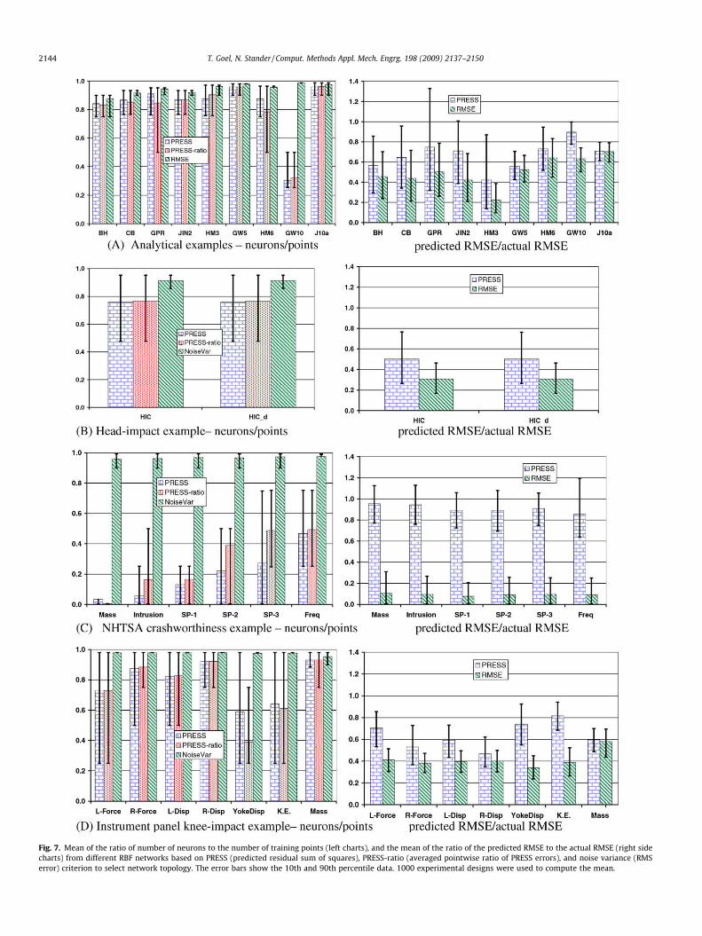
Fig. 7. Mean of the ratio of number of neurons to the number of training points (left charts), and the mean of the ratio of the predicted RMSE to the actual RMSE (right sidecharts) from different RBF networks based on PRESS (predicted residual sum of squares), PRESS-ratio (averaged pointwise ratio of PRESS errors), and noise variance (RMSerror) criterion to select network topology. The error bars show the 10th and 90th percentile data. 1000 experimental designs were used to compute the mean.


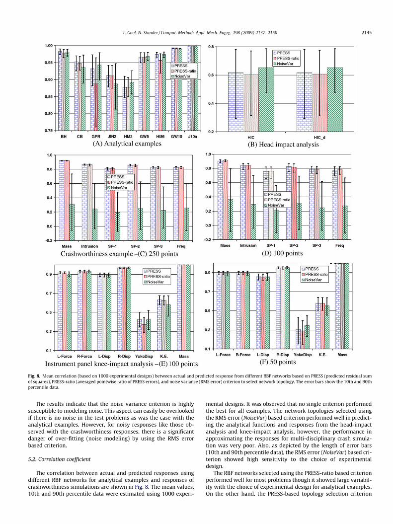
Fig. 8. Mean correlation (based on 1000 experimental designs) between actual and predicted response from different RBF networks based on PRESS (predicted residual sumof squares), PRESS-ratio (averaged pointwise ratio of PRESS errors), and noise variance (RMS error) criterion to select network topology. The error bars show the 10th and 90thpercentile data.


The results indicate that the noise variance criterion is highlysusceptible to modeling noise. This aspect can easily be overlookedif there is no noise in the test problems as was the case with theanalytical examples. However, for noisy responses like those ob-served with the crashworthiness responses, there is a significantdanger of over-fitting (noise modeling) by using the RMS errorbased criterion.

5.2. Correlation coefficient

The correlation between actual and predicted responses usingdifferent RBF networks for analytical examples and responses ofcrashworthiness simulations are shown in Fig. 8. The mean values,10th and 90th percentile data were estimated using 1000 experi-

mental designs. It was observed that no single criterion performedthe best for all examples. The network topologies selected usingthe RMS error (NoiseVar) based criterion performed well in predict-ing the analytical functions and responses from the head-impactanalysis and knee-impact analysis, however, the performance inapproximating the responses for multi-disciplinary crash simula-tion was very poor. Also, as depicted by the length of error bars(10th and 90th percentile data), the RMS error (NoiseVar) based cri-terion showed high sensitivity to the choice of experimentaldesign.

The RBF networks selected using the PRESS-ratio based criterionperformed well for most problems though it showed large variabil-ity with the choice of experimental design for analytical examples.On the other hand, the PRESS-based topology selection criterion

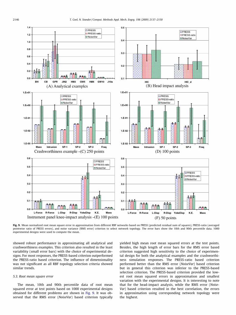
Fig. 9. Mean normalized root mean square error in approximation from different RBF networks based on PRESS (predicted residual sum of squares), PRESS-ratio (averagedpointwise ratio of PRESS errors), and noise variance (RMS error) criterion to select network topology. The error bars show the 10th and 90th percentile data. 1000experimental designs were used to compute the mean.


showed robust performance in approximating all analytical andcrashworthiness examples. This criterion also resulted in the leastvariability (small error bars) with the choice of experimental de-signs. For most responses, the PRESS-based criterion outperformedthe PRESS-ratio based criterion. The influence of dimensionalitywas not significant as all RBF topology selection criteria showedsimilar trends.

5.3. Root mean square error

The mean, 10th and 90th percentile data of root meansquared error at test points based on 1000 experimental designsobtained for different problems are shown in Fig. 9. It was ob-served that the RMS error (NoiseVar) based criterion typically

yielded high mean root mean squared errors at the test points.Besides, the high length of error bars for the RMS error basedcriterion suggested high sensitivity to the choice of experimen-tal design for both the analytical examples and the crashworthi-ness simulation responses. The PRESS-ratio based criterionperformed better than the RMS error (NoiseVar) based criterionbut in general this criterion was inferior to the PRESS-basedselection criterion. The PRESS-based criterion provided the low-est root mean squared errors in approximation and smallestvariation with the experimental designs. It is interesting to notethat for the head-impact analysis, while the RMS error (Noise-Var) based criterion resulted in the best correlation, the errorsin approximation using corresponding network topology werethe highest.

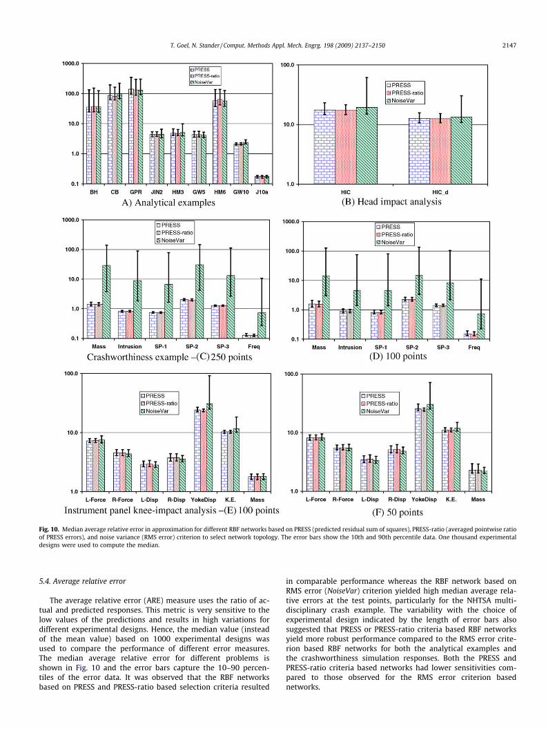
Fig. 10. Median average relative error in approximation for different RBF networks based on PRESS (predicted residual sum of squares), PRESS-ratio (averaged pointwise ratioof PRESS errors), and noise variance (RMS error) criterion to select network topology. The error bars show the 10th and 90th percentile data. One thousand experimentaldesigns were used to compute the median.


5.4. Average relative error

The average relative error (ARE) measure uses the ratio of ac-tual and predicted responses. This metric is very sensitive to thelow values of the predictions and results in high variations fordifferent experimental designs. Hence, the median value (insteadof the mean value) based on 1000 experimental designs wasused to compare the performance of different error measures.The median average relative error for different problems isshown in Fig. 10 and the error bars capture the 10–90 percen-tiles of the error data. It was observed that the RBF networksbased on PRESS and PRESS-ratio based selection criteria resulted

in comparable performance whereas the RBF network based onRMS error (NoiseVar) criterion yielded high median average rela-tive errors at the test points, particularly for the NHTSA multi-disciplinary crash example. The variability with the choice ofexperimental design indicated by the length of error bars alsosuggested that PRESS or PRESS-ratio criteria based RBF networksyield more robust performance compared to the RMS error crite-rion based RBF networks for both the analytical examples andthe crashworthiness simulation responses. Both the PRESS andPRESS-ratio criteria based networks had lower sensitivities com-pared to those observed for the RMS error criterion basednetworks.

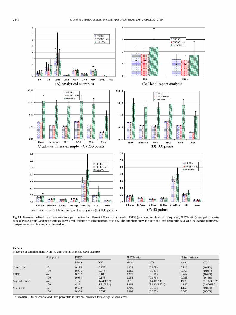
Fig. 11. Mean normalized maximum error in approximation for different RBF networks based on PRESS (predicted residual sum of squares), PRESS-ratio (averaged pointwiseratio of PRESS errors), and noise variance (RMS error) criterion to select network topology. The error bars show the 10th and 90th percentile data. One thousand experimentaldesigns were used to compute the median.

Table 9Influence of sampling density on the approximation of the GW5 example.

# of points PRESS PRESS-ratio Noise variance

Mean COV Mean COV Mean COV

Correlation 42 0.336 (0.572) 0.324 (0.603) 0.317 (0.482)100 0.966 (0.014) 0.966 (0.013) 0.969 (0.011)

RMSE 42 0.207 (0.106) 0.220 (0.321) 0.262 (0.473)100 0.055 (0.178) 0.055 (0.176) 0.053 (0.166)

Avg. rel. errora 42 16.2 (14.4/17.2) 16.1 (14.4/17.1) 19.7 (16.1/35.32)100 4.35 (3.61/5.52) 4.355 (3.610/5.521) 4.180 (3.470/5.211)

Max error 42 0.698 (0.160) 0.796 (0.585) 1.155 (0.884)100 0.308 (0.337) 0.308 (0.335) 0.303 (0.335)

a Median, 10th percentile and 90th percentile results are provided for average relative error.



5.5. Maximum absolute error

The results obtained for root mean square approximation errorswere also valid for the maximum absolute error test metric(Fig. 11).

It can be concluded that the PRESS criterion to select networktopology yielded robust and the best performance for all analyticaland crashworthiness simulation responses. Other criteria (PRESS-ratio and RMS error based criteria) performed well for selected re-sponses only and were more susceptible to the nature of theunderlying response and the choice of experimental designs. It isnoted that the PRESS criterion can be used with any strategy to se-lect RBF network topology.

5.6. Influence of sampling density

Since crashworthiness computations are expensive, mostapproximations are carried out using data from a few simulations.It is important to compare the three RBF topology selection criteriafor a small number of data points.

The analytical example GW5 was approximated with 42 pointsand predictions were carried out at the same set of test points. Themean and coefficient of variation of correlation, RMS error andmaximum absolute error, and median and 10–90th percentileaverage relative error based on 1000 experimental designs werecompared with the approximations based on 100 points in Table9. As expected, low point density resulted in higher RMS and max-imum errors, and lower correlation compared to the approxima-tion based on 100 points. Nevertheless, the PRESS-based criterionperformed significantly better (higher correlation, lower errors,lower coefficient of variations) than the PRESS-ratio and RMS error(NoiseVar) based criterion among all RBF networks constructedusing the same number of design points. It is important to notethat this example did not have any noise so the results for theRBF network selected using the NoiseVar criterion were not ad-versely affected.

To assess the influence of low sampling density on crashworthi-ness simulations, the multi-disciplinary crashworthiness examplewas approximated with 100 points and the IP structure knee im-pact problem was modeled using 50 points. The correlation, RMS,average relative, and maximum errors for the two examples withreduced sampling density are shown in Figs. 8–11. Comparingthe MDO crashworthiness example results from Fig. 8C, Fig. 9C,Fig. 10C, Fig. 11C (250 points experimental design) and Fig. 8D,Fig. 9D, Fig. 10D, Fig. 11D (100 points experimental design); andthe knee-impact example results from Fig. 8E, Fig. 9E, Fig. 10E,Fig. 11E (100 points experimental design) and Fig. 8F, Fig. 9F,Fig. 10F, Fig. 11F (50 points experimental design), it can be con-cluded that the PRESS based criterion was the best and the RMS er-ror (NoiseVar) based criterion was the worst even when a smallernumber of points was available. As expected, the approximationsbased on higher sampling density were mostly better (higher cor-relation, lower errors, smaller range depicted by 10–90 percentiles)however, the quality of the approximations for some responses(e.g., SP2 for NHTSA example) improved with reduction in sam-pling density when the RMS error (NoiseVar) criterion was usedto optimize RBF topology. This behavior is attributed to the noisein response.

Fig. 12. Comparing direct and equivalent computation of pointwise PRESS errors.

6. Conclusions

In this study, three criteria to select optimal RBF network topol-ogy for crashworthiness response approximation were comparedusing a number of analytical and crashworthiness simulation prob-lems ranging from two to eleven variables. The influence of sam-

pling density and choice of experimental designs were assessedsimultaneously. PRESS or PRESS-ratio criteria based RBF networkshad fewer neurons compared to the network determined usingthe RMS error (NoiseVar) criterion. The results indicated that thechoice of best network topology selection criterion depends onthe problem and experimental design. However, the PRESS-basedcriterion to select RBF network topology resulted in the robust per-formance for all examples, experimental designs, and samplingdensities. The PRESS-ratio based selection criterion also performedreasonably well, but it had high sensitivity to the choice of exper-imental design for the analytical examples. Often the network se-lected using the PRESS criterion, outperformed the networkselected using the PRESS-ratio based criterion. It was observed thatthe RMS error (NoiseVar) based criterion was the worst of the threecriteria for crashworthiness response approximation. The perfor-mance of the RMS error based criterion was very sensitive to thechoice of experimental design and sampling density. Also withthe increase in the number of points used for approximation, theRMS error selection criterion resulted in networks that over-fittedthe data. In summary, the PRESS-based selection criterion is rec-ommended for the selection of network topologies. This resultagrees with the studies by Sanchez et al. [46], and Viana and Haftka[47] who concluded that PRESS is a good criterion to select highquality approximations. The PRESS criterion has therefore beenchosen as the default criterion for RBF topology selection in LS-OPT�.

Acknowledgements

Authors sincerely thank Prof. Raphael Haftka and the reviewersfor their constructive comments that significantly improved thispaper.

Appendix. Verifying the accuracy of computations

PRESS error at some design point is evaluated using Eq. (11). Forlarge number of points, there is potential of ill-conditioning of theP matrix and hence the singular value decomposition based meth-odology adopted here [20] may result in wrong results. The accu-racy of pointwise PRESS error computation was verified bycomparing the results from the methodology with an exact compu-tation (P matrix was constructed in MATLAB and direct inverse wasused to compute pointwise PRESS errors). A single experimentaldesign for analytical example GW10, that was approximated using150 points, was used. The pointwise PRESS error values from the


two approaches are plotted in Fig. 12. The maximum absolute dif-ference in results was 2.8079e�10 (2.5025e�8%). It is clear thatthe methodology used in this paper accurately calculates pointwisePRESS errors.

References

[1] A.J. Kurdila, J.L. Peterson, Adaptation of centers of approximation for nonlineartracking control, J. Guidance Control Dyn. 19 (2) (1996) 363–369.

[2] Y. Li, N. Sundarajan, P. Saratchandran, Stable neuro-flight controller using fullytuned radial basis function neural networks, J. Guidance Control Dyn. 24 (4)(2001).

[3] A. Young, C. Cao, V. Patel, N. Hovakimyan, E. Lavertsky, Adaptive control designmethodology for nonlinear-in-control systems in aircraft application, J.Guidance Control Dyn. 30 (6) (2007).

[4] K.R. Wheeler, A.P. Dhawan, C.M. Meyer, Space shuttle main engine sensormodeling using radial basis function neural networks, J. Spacecraft Rockets 31(6) (1994) 1054–1060.

[5] N. Papila, W. Shyy, L. Griffin, D.J. Dorney, Shape optimization of supersonicturbines using global approximation methods, J. Prop. Power 18 (3) (2002)509–518.

[6] W. Shyy, N. Papila, R. Vaidyanathan, K. Tucker, Global design optimization foraerodynamics and rocket propulsion components, Prog. Aerospace Sci. 37 (1)(2001) 59–118.

[7] M.K. Karakasis, K.C. Giannakoglou, On the use of metamodel assisted multi-objective evolutionary algorithms, Engrg. Optim. 38 (8) (2006) 941–957.

[8] M. Meckesheimer, R.R. Barton, T. Simpson, F. Limayen, B. Yannou,Metamodeling of discrete/continuous responses, AIAA J. 39 (10) (2001)1950–1959.

[9] H. Rocha, W. Li, A. Hahn, Principal component regression for fitting wingweight data of subsonic transports, J. Aircraft 43 (6) (2006) 1925–1936.

[10] T. Zhang, K.K. Choi, S. Rahman, K. Cho, P. Baker, M. Shakil, D. Heitkamp, Ahybrid surrogate and pattern search optimization method and application tomicroelectronics, Struct. Multidiscip. Optim. 32 (4) (2006) 327–345.

[11] R.R.K. Reddy, R. Ganguli, Structural damage detection in a helicopter rotorblade using radial basis function neural networks, Smart Mater. Struct. 12(2003) 232–241.

[12] B. Glaz, P.P. Friedmann, L. Liu, Surrogate based optimization of helicopter rotorblades for vibration reduction in forward flight, Struct. Multidiscip. Optim. 35(4) (2008) 341–363.

[13] S.S. Panda, D. Chakraborty, S.K. Pal, Flank wear prediction in drilling using backpropagation neural networks and radial basis function network, Appl. SoftComput. 8 (2) (2008) 858–871.

[14] L. Lanzi, L.M.L. Castelletti, M. Anghileri, Multi-objective optimization ofcomposite absorber shape under crashworthiness requirements, Compos.Struct. 65 (3–4) (2004) 433–441.

[15] H. Fang, M. Rais-Rohani, A. Liu, M.F. Horstemeyer, A comparative study ofmetamodeling methods for multi-objective crashworthiness optimization,Comput. Struct. 83 (25–26) (2005) 2121–2136.

[16] M.J.L. Orr, Local Smoothing of Radial Basis Function Networks, Center forCognitive Science, University of Edinburgh, 1995.

[17] M.J.L. Orr, Regularization in the Selection of Radial Basis Function, CentersCenter for Cognitive Science, University of Edinburgh, 1995.

[18] M.J.L. Orr, Introduction to Radial Basis Function Networks, Center for CognitiveScience, University of Edinburgh, 1996.

[19] M.J.L. Orr, Optimizing the Widths of Radial Basis Functions, Center forCognitive Science, University of Edinburgh, 1998.

[20] M.J.L. Orr, Recent Advances in Radial Basis Function Networks, Institute ofAdaptive and Neural Computation, University of Edinburgh, 1999.

[21] J. Utans, J. Moody, Selecting neural network architecture via the predictionrisk: application to corporate bond rating prediction, in: Proceedings of theFirst International Conference on Artificial Intelligence Applications on WallStreet, IEEE Computer Society Press, Los Alamitos CA, 1991.

[22] P. Zhang, Model selection via multifold cross validation, Ann. Stat. 21 (1)(1993) 299–313.

[23] J. Moody, J. Utans, Architecture selection strategies for neural networks:application to corporate bond rating prediction, in: , A.N. Refenes (Ed.), NeuralNetworks in the Capital Markets, Wiley, 1994.

[24] T. Anderson, T. Martinez, Cross validation and MLP architecture selection,Neural Networks 3 (1999) 1614–1619.

[25] C.E. Vasios, G.K. Matsopoulos, E.M. Ventouras, K.S. Nikita, N. Uzunoglu, Cross-validation and neural network architecture selection for the classification ofintracranial current sources, in: Proceedings of 7th Neural NetworkApplications in Electrical Engineering (NEUREL 2004), Belgrade, September2004, pp. 151–185.

[26] S. Chen, C.F.N. Cowan, P.M. Grant, Orthogonal least squares learning algorithmfor radial basis function networks, IEEE Transactions on Neural Networks 2 (2)(1991) 302–309.

[27] A.A. Mullur, A. Messac, Extended radial basis functions: more flexible andeffective metamodeling, AIAA J. 43 (6) (2005) 1306–1315.

[28] R.L. Hardy, Multiquadrics equations of topography and other irregularsurfaces, J. Geophys. Res. 76 (1991) 1905–1915.

[29] A.N. Tikhonov, V.Y. Arsenin, Solutions to Ill-Posed Problems, Wiley, New York,1977.

[30] G. Golub, M. Heath, G. Wahba, Generalized cross-validation as a method forchoosing a good ridge parameter, Technometrics 21 (2) (1979) 215–223.

[31] G.H. Golub, U. von Matt, Generalized cross-validation for large scale problems,J. Comput. Graphical Stat. 6 (1) (1997) 1–34.

[32] N. Stander, W. Roux, T. Goel, T. Eggleston, K. Craig, LS-OPT Manual, vol. 3.4,Livermore Software Technology Corporation, Livermore CA, 2007.

[33] T. Goel, R.T. Haftka, W. Shyy, N.V. Queipo, Ensemble of Surrogates, Struct.Multidiscip. Optim. 33 (2007) 199–216.

[34] T. Goel, R.T. Haftka, W. Shyy, Error measures on surrogate approximationbased on noise-free data, in: Proceedings of 46th AIA Aerospace SciencesMeeting and Exhibit, Reno NV, 2008, AIAA-2008-0901.

[35] L.C.W. Dixon, G.P. Szego, Towards Global Optimization, vol. 2, North Holland,Amsterdam, 1978.

[36] R. Jin, W. Chen, T. Simpson, Comparative studies of metamodeling techniquesunder multiple modeling criteria, Struct. Multidiscip. Optim. 23 (1) (2001)385–398.

[37] A.A. Giunta, L.T. Watson, A comparison of approximation modelingtechniques: polynomial versus interpolating models, in: Proceedings of 7thAIAA/UAF/NASA/ISSMO Symposium on Multidisciplinary Analysis andOptimization, St. Louis MO, 1998, AIAA-98-4758.

[38] K.J. Craig, N. Stander, D.A. Dooge, S. Varadappa, Automotive crashworthinessdesign using response surface-based variable screening and optimization,Engrg. Optim. 22 (1) (2005) 38–61.

[39] National Crash Analysis Center (NCAC), Public Finite Element Model Archive,2001. <www.ncac.gmu.edu/archives/model/index.html>.

[40] Livermore Software Technology Corporation, LS-Dyna Manual, vol. 971,Livermore CA, 2007.

[41] A. Akkerman, R. Thyagarajan, N. Stander, M. Burger, R. Kuhm, H. Rajic, Shapeoptimization for crashworthiness design using response surfaces, in:Proceedings of the International Workshop on Multidisciplinary DesignOptimization, Pretoria SA, 2000, pp. 270–279.

[42] C.W. Ueberhuber, Numerical computation 2: methods, software, and analysis,Springer, New York, p 71.

[43] R.H. Myers, D.C. Montgomery, Response Surface Methodology, Wiley, NewYork, 2002.

[44] T. Goel, R.T. Haftka, W. Shyy, L.T. Watson, Pitfalls of using a single criterion forselecting experimental designs, Int. J. Numer. Methods Engrg. 75 (2) (2008)127–155.

[45] G. Li, T. Goel, N. Stander, Assessing the convergence properties of NSGA-II fordirect crashworthiness optimization, in: Proceedings of the 10th InternationalLS-DYNA Users Conference, Detroit MI, June, 2008, pp. 8–10.

[46] E. Sanchez, S. Pintos, N.V. Queipo, Toward an optimal ensemble of kernel-based approximations with engineering applications, Struct. Multidiscip.Optim. 36 (3) (2008) 247–261.

[47] F.A.C. Viana, R.T. Haftka, Using multiple surrogates for minimization of theRMS error in meta-modeling, in: Proceedings of the ASME 2008 InternationalDesign Engineering Technical Conferences & Computers and Information inEngineering Conference – IDETC/CIE 2008, New York NY, August 3–6, 2008.

http://www.ncac.gmu.edu/archives/model/index.html

comparing three error criteria for selecting radial basis function network topology

Documents