comparing subsidies, loans, and standards for improving

253Cityscape: A Journal of Policy Development and Research • Volume 16, Number 1 • 2014U.S. Department of Housing and Urban Development • Office of Policy Development and Research

Cityscape

Comparing Subsidies, Loans, and Standards for Improving Home Energy EfficiencyMargaret WallsResources for the Future

Abstract

Residential buildings use approximately 20 percent of the total U.S. energy consump-tion, and single-family homes alone account for about 16 percent. Older homes are less energy efficient than newer ones, and, although many experts have identified upgrades and improvements that can yield significant energy savings at relatively low costs, it has proven to be difficult to spur most homeowners into making these investments. In this article, I analyze the energy and carbon dioxide (CO

2) effects from three policies aimed

at improving home energy efficiency: (1) a subsidy for the purchase of efficient space heating, cooling, and water-heating equipment; (2) a loan for the same purchases; and (3) efficiency standards for such equipment. I use a version of the U.S. Department of Energy (DOE), Energy Information Administration’s (EIA’s) National Energy Modeling System, NEMS-RFF,1 to compute the energy and CO

2 effects and standard formulas in

economics to calculate the welfare costs of the policies. I find that the loan option is quite cost effective but provides only a very small reduction in CO

2 emissions and energy use.

The subsidy and the standards both are more costly but generate CO2 emissions reduc-

tions seven times greater than the loan option. The subsidy promotes consumer adoption of very high-efficiency equipment, but the standards do not; they lead to purchases of equipment that just reaches the standards. The discount rate used to discount energy savings from the policies has a large effect on the welfare cost estimates.

1 RFF in NEMS-RFF stands for Resources for the Future, as the small changes to the model inputs and assumptions were made for modeling runs completed for Resources for the Future. The views expressed in this article do not necessarily reflect the views of EIA or DOE. EIA makes the model available for use by others, but only select firms and some academics have the expertise to run the model. OnLocation, Inc. (http://www.onlocationinc.com/) ran NEMS-RFF for the purposes of this study.

http://www.onlocationinc.com/

254

Walls

Refereed Papers

IntroductionCommercial and residential buildings account for 42 percent of energy consumption in the United States, and residential buildings alone are responsible for one-half of this amount. Building codes, appliance standards, and general technological improvements have vastly improved the energy ef - ficiency of new homes, but older homes lag behind newer homes in efficiency. A home built in the 1940s consumes, on average, 50.8 thousand British thermal units (Btus) per square foot, even with improvements made since it was built. An average home built in the 1990s, on the other hand, con - sumes only 37.7 thousand Btus per square foot (DOE/EIA, 2008). With 75 percent of the existing housing stock built before 1990, to make a serious dent in residential energy consumption will require policies that target retrofit and upgrade options to existing properties.

Experts have disagreed about the best approaches for spurring homeowners to use retrofit options, and current policy takes a somewhat scattershot approach. Since the mid-1980s, the federal govern - ment has set mandatory minimum efficiency standards for a variety of appliances and equipment and, in President Barack Obama’s June 2013 Climate Action Plan, he proposed tightening those standards for a number of products (Executive Office of the President, 2013). In addition, the gov - ernment operates the voluntary ENERGY STAR certification program for equipment and new homes that reach even higher levels of efficiency. Many state and local governments encourage building retrofit options in a variety of ways. Approximately 250 energy-efficiency-financing programs are in operation at the state, local, and utility level (Palmer, Walls, and Gerarden, 2012). These programs provide low-interest loans to consumers (and businesses) who upgrade their properties. The Rural Utilities Service also has long operated an energy-efficiency loan program, implemented by rural electric cooperatives, and President Obama also proposed an increase to this program (Executive Office of the President, 2013). Tax credits, rebates, and direct subsidies have also been available to varying degrees in different locations and at different times; in fact, these financial incentives were key components of the 2009 American Recovery and Reinvestment Act stimulus bill. Also, some cities recently adopted energy-disclosure requirements for commercial and multifamily residential buildings, on the premise that making energy information publicly available will spur improvements.

Studies of the effectiveness and cost effectiveness of policies that focus on end-use energy efficiency are limited. The often cited McKinsey & Company (2009) report identifies a number of building retrofit options with discounted streams of energy savings that more than offset the upfront costs of the improvements. These measures would purportedly yield 12.4 quadrillion Btus in energy savings in 2020, 29 percent of predicted baseline energy use in buildings in that year. The study does not describe or analyze policy options that will bring these changes about, however. A similar comment can be made about a 2010 National Academy of Sciences study (NAS, 2010). Brown et al. (2009) do focus on policies; they look at building codes, energy-performance-rating systems, mandated disclosure of energy use, and “on-bill” energy-efficiency-financing programs, as well as three poli-cies targeted to utilities. The authors estimate energy savings and costs for each option, but these estimates are based on the authors’ assumptions and results from other studies, not from detailed statistical or simulation modeling. Krupnick et al. (2010) estimate the costs and effectiveness of a variety of policies to reduce energy use and carbon dioxide (CO

2) emissions, including four

end-use energy-efficiency policies: building energy codes; building energy codes combined with other policies, as specified in the 2009 Waxman-Markey climate bill (H.R. 2454); and two smaller

Comparing Subsidies, Loans, and Standards for Improving Home Energy Efficiency

255Cityscape

scale policies, one using a subsidy and the other a loan, for the purchase of geothermal heat pumps (GHPs). Krupnick et al. (2010) use a version of the National Energy Modeling System (NEMS), the market equilibrium simulation model used by the U.S. Department of Energy (DOE)/Energy Infor-mation Administration (EIA) for its short- and long-term energy-use forecasts (DOE/EIA, 2011) to have a consistent framework with which to evaluate energy and CO

2 reductions across policies. The

authors then use standard methodologies from public economics to calculate the costs of each policy.

This article takes an approach similar to that of Krupnick et al. (2010), using a version of NEMS (NEMS-RFF, in which small changes to the NEMS inputs and assumptions were made for model-ing runs completed for Resources for the Future) to analyze three policy options to reduce home energy use—two incentive-based instruments and a command-and-control approach. The study focuses on heating and air-conditioning equipment and water heaters, which together account for approximately 70 percent of an average home’s energy use. I compare a subsidy for the purchase of high-efficiency equipment with a zero-interest loan of the same initial amount. I then contrast these two economic incentive-based policies with a policy that is of a more command-and-control nature—efficiency standards for new equipment.

NEMS-RFF has a high level of technological detail in the four end-use energy sectors—residential, commercial, industrial, and transportation—as well as the electricity sector, making possible detailed modeling of alternative policies. By using a consistent modeling framework with the same baseline assumptions for comparison, I am able to make an apples-to-apples comparison of the three policy options and contrast the results to those in Krupnick et al. (2010). I also can compare with baseline forecasts that are consistent with EIA’s Annual Energy Outlook (AEO). I use model output to calculate the welfare costs of the policies; this approach, in turn, enables me to estimate the cost effectiveness of each policy in reducing CO

2 emissions—that is, the welfare costs per ton

of CO2 emissions reduced.

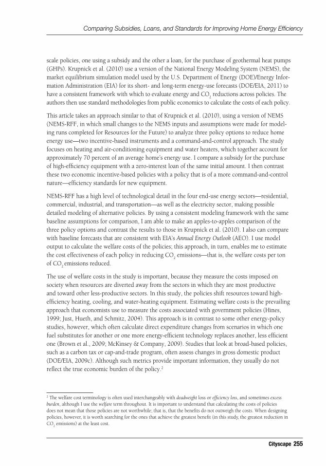
The use of welfare costs in the study is important, because they measure the costs imposed on society when resources are diverted away from the sectors in which they are most productive and toward other less-productive sectors. In this study, the policies shift resources toward high-efficiency heating, cooling, and water-heating equipment. Estimating welfare costs is the prevailing approach that economists use to measure the costs associated with government policies (Hines, 1999; Just, Hueth, and Schmitz, 2004). This approach is in contrast to some other energy-policy studies, however, which often calculate direct expenditure changes from scenarios in which one fuel substitutes for another or one more energy-efficient technology replaces another, less efficient one (Brown et al., 2009; McKinsey & Company, 2009). Studies that look at broad-based policies, such as a carbon tax or cap-and-trade program, often assess changes in gross domestic product (DOE/EIA, 2009c). Although such metrics provide important information, they usually do not reflect the true economic burden of the policy.2

2 The welfare cost terminology is often used interchangeably with deadweight loss or efficiency loss, and sometimes excess burden, although I use the welfare term throughout. It is important to understand that calculating the costs of policies does not mean that those policies are not worthwhile; that is, that the benefits do not outweigh the costs. When designing policies, however, it is worth searching for the ones that achieve the greatest benefit (in this study, the greatest reduction in CO

2 emissions) at the least cost.

256

Walls

Refereed Papers

I find the loan policy to be more cost effective than the subsidy, and, with low enough discount rates, the costs are even negative—that is, the discounted stream of future energy savings offsets the welfare cost in the equipment market to generate an overall negative net welfare cost. The loan achieves only a very small reduction in energy use and CO

2 emissions, however. The financial

incentive to switch to high-efficiency equipment options is simply not that great because the loan has to be repaid. This result appears to be consistent with findings in the loan programs that have been operated to date, which have had quite low participation rates (Palmer, Walls, and Gerarden, 2012). Consumers respond more to the subsidy, and thus energy and CO

2 emissions reductions

are much greater with this policy. CO2 reductions are more than seven times greater than with the

loan. This policy comes with higher welfare costs, however; thus, policymakers face a tradeoff.

The modeling results show the efficiency standards achieving CO2 emissions and energy reductions

approximately equal to those of the subsidy, but the costs of this policy option are greater. This finding highlights the importance of using a measure of welfare costs to analyze policies. Because a standard essentially removes a large number of product choices from the marketplace—all of the relatively low-efficiency space heating and cooling and water-heating equipment—it generates a larger welfare cost than the subsidy. Moreover, because the subsidy incentivizes purchases of all high-efficiency equipment, including the very high-efficiency but higher cost options, it generates somewhat greater CO

2 emissions reductions per dollar of welfare cost. The standard leads to more

equipment that just meets the level of the standard.

The loan and subsidy policies compare favorably on a cost-effectiveness basis with the policies analyzed in Krupnick et al. (2010), with the exception of the broad cap-and-trade and carbon tax policies. In particular, they are more effective than building energy codes—that is, they provide a greater reduction in CO

2 emissions—primarily because they have a more immediate effect, where-

as building codes provide energy and CO2 reductions more gradually as new buildings replace

older ones. On a cost-effectiveness basis, the building codes and subsidy policy are very similar. The subsidy is less cost effective than some other approaches, such as a clean-energy standard applied to electricity generation, but the very low cost of the loan option makes it compare favor-ably with almost all other options analyzed in the Krupnick et al. (2010) study,3 although, again, it achieves very small reductions in CO

2 emissions. It is interesting that Krupnick et al. (2010)

look at subsidies and loans for geothermal heat pumps, a very high-efficiency but high-cost space heating and cooling option, and find the policies were more cost effective than the more broadly applied policies analyzed in this article. These results suggest that, if the government is going to implement energy-efficiency policies, careful targeting of those policies may be appropriate from a cost-effectiveness standpoint.

In this article, the following section describes NEMS-RFF, with special attention to the residential module and how heating and air-conditioning equipment and water heaters are incorporated in the model. The subsequent section shows baseline results—forecasts of annual residential-sector energy consumption and CO

2 emissions to 2035 and the distribution of technologies in use during

the period under a business-as-usual scenario. The next section describes the specific loan and

3 A clean-energy standard requires electric utilities to use a certain share of clean sources of fuel (for example, wind, solar, nuclear, and sometimes natural gas) for the electricity they produce (see Mignone et al., 2012).


257Cityscape

subsidy policies and shows results from the model, along with the welfare cost calculations. I then compare the subsidy results with an equivalent technology standard in the section that follows. The penultimate section compares my cost-effectiveness results for the three energy-efficiency poli-cies with cost-effectiveness estimates for alternative policies from other studies. The final section provides some concluding remarks.

The NEMS-RFF ModelNEMS is the primary model that the U.S. Energy Information Administration uses in its Annual Energy Outlook forecasts of future energy prices, supply, and demand (DOE/EIA, 2011). Some model modifications were made to represent the policy cases, thus we refer to the model through-out as NEMS-RFF. In this section, we provide a brief overview of the model.

Model OverviewNEMS-RFF is an energy-systems model, also often referred to as a bottom-up model. As in most energy-systems models, NEMS-RFF incorporates considerable detail on a wide spectrum of exist-ing and emerging technologies across the energy system, while also balancing supply and demand in all (energy and other) markets. The model is modular in nature (exhibit 1), with each module representing individual fuel supply, conversion, and end-use consumption. The model solves

Exhibit 1

Visual Representation of NEMS

NEMS = National Energy Modeling System.

Source: DOE/EIA (2009a)

Oil and gassupply module

Natural gas transmission

and distribution module

Coal market module

Renewable fuels module

Supply Conversion Demand

Macroeconomic activity module

Electricity market module

Petroleum market module

International energy module

Residential demand module

Commercial demand module

Transportation demand module

Industrial demand module

Integrating Module

258

Walls

Refereed Papers

iteratively until the delivered prices of energy are in equilibrium. Many of the modules contain ex-tensive data: industrial demand is represented for 21 industry groups, for example, and light-duty vehicles are disaggregated into 12 classes and are distinguished by vintage. The model also has regional disaggregation, taking into account, for example, state electric utility regulations. It also incorporates existing regulations, taxes, and tax credits, all of which are updated regularly.

NEMS-RFF incorporates a fair amount of economic behavioral assumptions in its various modules. These assumptions allow for the model to be used to capture the effects of various economic incentive-based policies, such as taxes and subsidies. The model will also measure the effects policies that are of a more command-and-control nature have on some fuel and electricity prices, although the model has some limitations in this regard. Price elasticities of demand, payback periods for capital investments, and other economic factors are chosen based on extensive reviews of the literature and evidence from equipment and fuel markets.

The Residential ModuleThe NEMS-RFF Residential Sector Demand Module4 starts with exogenously given population and housing construction input data from the NEMS Macroeconomic Activity Module. The module contains housing and equipment stock flow algorithms, a technology choice and housing shell effi-ciency algorithm, end-use energy consumption, and distributed electricity generation. Equipment purchases are based on a nested choice methodology with the first stage determining the fuel and technology—for example, an electric heat pump or a natural gas furnace for space heating—for both new and replacement equipment. After the technology and fuel choice are selected, the second stage determines the efficiency of the equipment. Most equipment has several different efficiency types available in the model, and generally more efficient equipment has a higher upfront cost. Market shares of each type are based on installed capital and operating costs; parameters of these functions are calibrated to market data. It is possible to calculate observed discount rates from the model based on the calibrations; these rates can reach as high as 30 percent. For the space heating, cooling, and water-heating equipment, rates are approximately 20 percent. Thus, incentive-based policies directed at high-efficiency equipment are expected to have somewhat limited effects on consumer purchase behavior as these relatively high discount rates imply that consumers need to see a quick payback (large energy savings) from the more efficient equipment or they will not pur-chase it. This intrinsic feature of the NEMS-RFF model is based on the DOE-EIA study of observed consumer behavior.

4 For more detailed information, see DOE/EIA (2009b).


259Cityscape

For the policy analyses in this study, I modify the capital and operating costs of the different types of heating, cooling, and water-heating equipment, and this shifts the share of purchases toward the subsidized technology types (within the limits of the model structure). For the technology standard policy, I remove the lower efficiency options from the choice set, as explained in more detail in the following section. NEMS-RFF assumes consumers replace equipment when it wears out, using typical lifetimes observed in the marketplace. Thus, the policies spur consumers to buy equipment that is more efficient than what they otherwise would have purchased, but they do not lead them to replace equipment before it wears out. For this reason, it is possible that NEMS underestimates the energy and CO

2 emissions reduction effects of the policies, although the extent to which

consumers would replace earlier in response to the policies is unclear.

Space Heating and Cooling and Water-Heating Technologies in the ModelThe NEMS-RFF model incorporates six different fuel types for space heating—(1) natural gas, (2) electricity, (3) liquefied petroleum gas (LPG), (4) kerosene, (5) distillate heating oil, and (6) wood— and four different types of heating technologies—(1) heat pumps, (2) radiant heat, (3) forced-air furnaces, and (4) geothermal heat pumps, or GHPs. In 2010, nearly 54 percent of the space heat-ing equipment stock in place in the United States was natural gas forced-air furnaces. Electric heat pumps accounted for 9.5 percent. By 2035, the NEMS-RFF baseline predictions with no policy changes are that relatively more space heating will be supplied by natural gas forced air furnaces and electric heat pumps—the shares increase to 55.4 and 14.1 percent, respectively.

NEMS-RFF builds in five basic technology types for natural gas furnaces, each of which has dif-ferent efficiencies and costs that vary somewhat over time and by region of the country. Improve-ments over time are also built in for most of the other space heating technologies in the model, including the four basic types of electric heat pumps and the four different types of central air-conditioning systems. In addition, NEMS-RFF incorporates any federal tax credits that are in place for specific technologies (GHPs are an important example) and phases them out if the legislation specifies a particular date at which they sunset. NEMS-RFF also includes room air-conditioners, which account for 41.6 percent of the air-conditioning equipment stock in 2010. As I explain in the discussion of the policy scenarios that follow, the focus in this study is on forced-air furnaces, electric heat pumps, GHPs, and central air-conditioning systems.5 Exhibit 2 shows a breakdown of the different technology types in the NEMS-RFF model for the major sources of residential space heating and cooling and water heating. The high-efficiency models are the targets of these policies.6

5 Natural gas radiant heat makes up only about 7 percent of heating-equipment purchases in a given year, a percentage that is expected to decline in the future; that technology is not incentivized in the policy scenarios here.6 For ease of interpretation, I categorize the technologies, which in NEMS are distinguished by efficiency factors and costs, and give them the labels in exhibit 2.

260

Walls

Refereed Papers

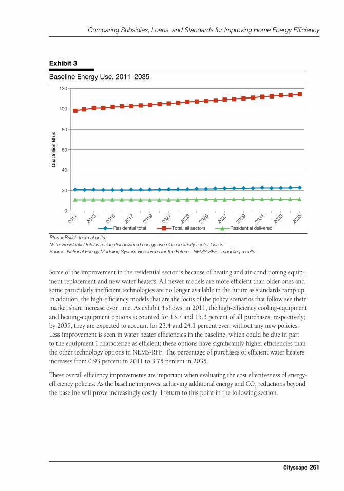
Baseline Modeling ResultsExhibit 3 shows the forecast of total energy consumption and residential energy consumption during the 2011-to-2035 forecast period under the baseline scenario. This baseline is consistent with the reference case in EIA’s 2011 AEO (DOE/EIA, 2011). As the exhibit makes clear, residential sector energy use—both delivered energy and total residential, including electricity sector losses—is pre - dicted to change very little, despite a forecasted growth of 28 percent in the number of U.S. house-holds by 2035. Delivered energy consumption is only 5.2 percent higher in 2035 than in 2011. This relatively small increase is because of improvements in energy efficiency in the building sector over time. The improvements result from the replacement of older equipment and appliances with newer, more efficient models and newly constructed houses that have improved building shells and other efficiency upgrades. Energy intensity in the residential sector—measured as millions of Btus of energy used per household—declines by more than 20 percent between 2010 and 2035. On a per-square-foot basis, energy intensity declines even more—by 31.3 percent during the 2010-to-2035 period.

Space Heating and Cooling Equipment Type Energy Efficiency

Exhibit 2

Space Heating and Cooling Technologies in the NEMS-RFF Model

Heat pumps HSPFLow-efficiency models 7.7High-efficiency models

Current ENERGY STAR 8.2Very high-efficiency ~ 9.5Ultra high-efficiency 10.7–10.9GHPs (all high-efficiency) 11.9–17.1

Natural gas, LPG, and oil furnaces AFUELow-efficiency models 80–83%High-efficiency models

Current ENERGY STAR 90%Very high-efficiency 96%

Central air-conditioners SEERLow-efficiency models 13.0–14.0High-efficiency models

Current ENERGY STAR 14.5Very high-efficiency 16.0Ultra high-efficiency 23.0

AFUE = annual fuel utilization efficiency. GHP = geothermal heat pump. HSPF = heating seasonal-performance factor. LPG = liquefied petroleum gas. NEMS = National Energy Modeling System. RFF = Resources for the Future. SEER = seasonal energy efficiency ratio.

Notes: HSPF measures a heat pump’s energy efficiency during one heating season. It is heating output, in British thermal units (Btus), divided by total electricity consumed in watt-hours. AFUE measures the amount of fuel converted to space heat in proportion to the amount entering the furnace; it is typically represented as a percentage. SEER measures an air-conditioner’s cooling output, in Btus, divided by total electric energy input in watt-hours. Information on ENERGY STAR requirements for heating, ventilation, and air-conditioning equipment, water heaters, and other equipment and appliances is available at http://www.energystar.gov/index.cfm?c=products.pr_find_es_products.

http://www.energystar.gov/index.cfm?c=products.pr_find_es_products


261Cityscape

Some of the improvement in the residential sector is because of heating and air-conditioning equip - ment replacement and new water heaters. All newer models are more efficient than older ones and some particularly inefficient technologies are no longer available in the future as standards ramp up. In addition, the high-efficiency models that are the focus of the policy scenarios that follow see their market share increase over time. As exhibit 4 shows, in 2011, the high-efficiency cooling-equipment and heating-equipment options accounted for 13.7 and 15.3 percent of all purchases, respectively; by 2035, they are expected to account for 23.4 and 24.1 percent even without any new policies. Less improvement is seen in water heater efficiencies in the baseline, which could be due in part to the equipment I characterize as efficient; these options have significantly higher effi ciencies than the other technology options in NEMS-RFF. The percentage of purchases of efficient water heaters increases from 0.93 percent in 2011 to 3.75 percent in 2035.

These overall efficiency improvements are important when evaluating the cost effectiveness of energy-efficiency policies. As the baseline improves, achieving additional energy and CO

2 reductions beyond

the baseline will prove increasingly costly. I return to this point in the following section.

120

0

20

40

2011

2013

2015

2017

2019

2021

2023

2025

2027

2029

2031

2033

2035

60

80

100

Residential total Total, all sectors Residential delivered

Qua

dri

llio

n B

tus

Exhibit 3

Baseline Energy Use, 2011–2035

Btus = British thermal units.

Note: Residential total is residential delivered energy use plus electricity sector losses.

Source: National Energy Modeling System-Resources for the Future—NEMS-RFF—modeling results

262

Walls

Refereed Papers

Loan and Subsidy Policy ScenariosThis section compares a subsidy for high-efficiency equipment with a zero-interest loan. The subsidy and loan are applied to all high-efficiency options, as specified in exhibit 2, and the high-efficiency water heaters. The modeled subsidy lowers the upfront capital cost of new and replace-ment equipment by 50 percent more than the baseline NEMS-RFF assumptions. This percentage reduction means that the dollar amount of the subsidy is larger for higher cost equipment and that the subsidy falls in size if costs come down over time, as occurs for some of the technologies in NEMS-RFF. I choose a subsidy of this magnitude in an effort to spur a significant move toward high-efficiency purchases in the policy scenarios, while acknowledging that a government subsidy (or tax credit) that would reduce prices by 50 percent may be unrealistic.7

The loan policy reduces the capital cost (to the equipment purchaser) by exactly the same amount as the subsidy, 50 percent of the baseline cost, but assumes that the loan is fully paid back during a 3-year period, with no interest. The 3-year period is arbitrary, but, because the loan amounts are not large and zero interest is charged on the loan, a relatively short payback period seems appro-priate. Most energy-efficiency loan programs that cover a wide range of home retrofit and upgrade options do not have a 0-percent interest rate; in fact, some loans have rates as high as 14 percent.8

13.7315.26

23.4224.10

0

5

10

15

20

25

0

10

20

30

40

50

60

Cooling

Per

cent

age

Per

cent

age

Heating

Cooling Heating Water heating

2011

Baseline Subsidy Loan

2035

20.622.2

3.2

50.847.9

39.7

33.529.5

5.5

Exhibit 4

High-Efficiency Heating and Cooling Equipment Sales As a Percentage of Total Sales, Baseline Case


7 Because running NEMS-RFF for alternative scenarios is time consuming and costly, I was unable to conduct sensitivity analyses with different-sized subsidies. In the results that follow, however, I do discuss how the cost effectiveness varies with discount rates, loan default rates, and other factors.8 The Fannie Mae Energy Loan program is one example. Many state and utility programs use the Fannie Mae program but buy down the interest rate to a more acceptable level, often about 7 percent (Palmer, Walls, and Gerarden, 2012).


263Cityscape

Thus, this zero-interest loan is a generous feature of the policy. On the other hand, 3 years is a relatively short term for the loan. Most energy-efficiency-financing programs have terms of around 10 years, although these longer terms are typically available only for much larger loans (Palmer, Walls, and Gerarden, 2012). In the NEMS-RFF model, the subsidy simply lowers the upfront equipment cost, leaving annual operating costs unchanged; the loan lowers the upfront cost by the same amount as the subsidy but effectively increases operating costs for the first 3 years of the equipment’s life. I assume a 2-percent default rate on loans. Existing loan programs have average default rates of less than 2 percent, but they tend to serve customers with very high credit scores.9 In a national program available to all consumers, one would expect the default rate to be higher.

Policy Modeling Results: Loans Versus SubsidiesBy lowering the purchase cost of high-efficiency heating, cooling, and water-heating equipment, the subsidy and the loan both shift purchases of new equipment toward the more efficient options over time. Exhibit 5 shows all efficient equipment purchases as a percentage of total equipment purchases during the 2011-to-2035 period. With the subsidy, more than one-half of all cooling equipment and nearly one-half of heating equipment purchased during this 25-year period are high-efficiency models; just less than 40 percent of water heaters are high-efficiency models. These increases are significant over the baseline case. Loans have less of an effect: high-efficiency cooling

9 Default rates on current loan programs are not widely available, but a program in Pennsylvania has had an average rate of 0.60 percent (State Energy Efficiency Action Network, 2011). The rate varies greatly by borrowers’ credit scores, however, and those with credit scores (FICO credit score model) of less than 650 have an average default rate of 4.33 percent.

13.7315.26

23.4224.10

0

5

10

15

20

25

0

10

20

30

40

50

60

Cooling

Per

cent

age

Per

cent

age

Heating

Cooling Heating Water heating

2011


2035

20.622.2

3.2

50.847.9

39.7

33.529.5

5.5

Exhibit 5

High-Efficiency Equipment Purchases, 2011–2035, As a Percentage of All Equipment Purchases


264

Walls

Refereed Papers

equipment purchases increase from 20.6 to 33.5 percent and high-efficiency heating equipment purchases increase from 22.2 to 29.5 percent. The loan policy has a much smaller effect on water heater purchases than does the subsidy.

As the new efficient equipment purchases gradually replace older equipment, energy use for heating and cooling declines relative to the baseline. Exhibit 6 shows residential delivered energy use during the 2011-to-2035 period under the baseline and the two policy cases. The subsidy has a much larger effect on residential energy use than does the loan. In fact, the loan is almost indistinguishable from the baseline. Neither policy has a large effect on energy use, however.10 By 2035, delivered energy use under the subsidy is 0.66 quadrillion Btus less than the baseline, a difference of only 5.6 percent.

Energy use eventually increases in all three scenarios because of population growth, but with the subsidy, total energy use in 2035 is slightly less than the 2011 level. Energy use falls, on a per-household basis, by 16.8 percent in the baseline between 2011 and 2035, by 17.4 percent with the loan, and by 21 percent with the subsidy. Thus the energy-efficiency policies work in reducing residential energy use, and accompanying CO

2 emissions, but the forces of population

and economic growth offset much of those reductions.

10 Note that the scale of the vertical axis is compressed in exhibit 6 so that the differences show up. By contrast, the scale in exhibit 3 is much wider.

P

P

0 S

P1 S’

D

Q0

Q1

Q

10.6

10.8

11.0

11.2

11.4

11.6

11.8

Qua

dri

llio

n B

tus

2011

2013

2015

2017

2019

2021

2023

2025

2027

2029

2031

2033

2035


Exhibit 6

Residential Delivered Energy Use, 2011–2035




265Cityscape

Cumulative energy-related CO2 emissions reductions during the 25-year forecast period from the

subsidy are 672.5 million metric tons (mmtons), seven times greater than the 94.9 mmton reduc-tion from the loan. With economywide CO

2 emissions during the same time period in the baseline

case at 148 billion metric tons, however, neither residential energy-efficiency policy makes a major dent in the problem, reducing CO

2 emissions by less than 0.5 percent in the case of the subsidy

and by a much smaller percentage with the loan. This result is expected: with heating, cooling, and water-heating equipment responsible for approximately 70 percent of the energy consumed in a residential building, and the residential sector as a whole accounting for approximately 20 percent of total energy use, these kinds of targeted energy-efficiency policies can make only a small contri-bution toward U.S. climate reduction goals. Nonetheless, in the absence of a broad-based carbon tax or cap-and-trade program, sector-specific policies may be the next-best solution, and thus it is important to assess their potential.

Welfare Costs and Cost Effectiveness of Loans and SubsidiesAs explained in the introduction, I focus on welfare costs to measure the economic burden of the policies rather than simple expenditure changes or other measures of costs. Welfare costs are the costs imposed on society when resources are diverted toward the production of high-efficiency heating, cooling, and water-heating equipment and away from other sectors in the economy.

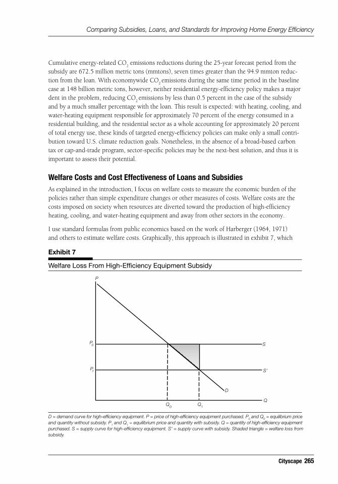
I use standard formulas from public economics based on the work of Harberger (1964, 1971) and others to estimate welfare costs. Graphically, this approach is illustrated in exhibit 7, which

P

P

0 S

P1 S’

D

Q0

Q1

Q

10.6

10.8

11.0

11.2

11.4

11.6

11.8

Qua

dri

llio

n B

tus

2011

2013

2015

2017

2019

2021

2023

2025

2027

2029

2031

2033

2035


Exhibit 7

Welfare Loss From High-Efficiency Equipment Subsidy

D = demand curve for high-efficiency equipment. P = price of high-efficiency equipment purchased. P0 and Q0 = equilibrium price and quantity without subsidy. P1 and Q1 = equilibrium price and quantity with subsidy. Q = quantity of high-efficiency equipment purchased. S = supply curve for high-efficiency equipment. S’ = supply curve with subsidy. Shaded triangle = welfare loss from subsidy.

266

Walls

Refereed Papers

shows the market for efficient heating, cooling, and water-heating equipment. The supply curve, S, shows the additional units of high-efficiency equipment, Q, that will be supplied to the market as the price, P, increases.11 The subsidy is shown as a horizontal shift downward in the supply curve. It lowers the net price to consumers, from P

0 to P

1, and it leads to a greater quantity purchased in

equilibrium, Q1. Consumers are better off as the subsidy lowers the purchase price they pay, but

the shift of resources to this sector of the economy and away from other sectors imposes a welfare cost equal to the shaded triangle. This area measures the additional government subsidy payments above and beyond the benefit to consumers from lower prices.12

I treat the loan policy as having exactly the same effect in the market for high-efficiency equip-ment, but the loan shifts the supply curve downward by a smaller amount than does the subsidy. Rather than shifting it down by the per-dollar subsidy amount, it shifts it down by the discounted present value of the forgone interest earnings on the loan. I compute this value using a 5-percent interest rate and the 3-year loan term. The welfare losses for both policies are calculated for each forecast year and the discounted present value of these losses is then computed using a 5-percent discount rate.13

One final adjustment to the welfare cost calculations is important. If one believes that a market failure exists in the market for energy efficiency because of information barriers, myopic consumers, credit rationing, risk, and uncertainty about new types of equipment, or any of a host of other rea-sons for the so-called efficiency gap, or energy paradox (Alcott and Greenstone, 2012; Gillingham, Newell, and Palmer, 2009; Jaffe and Stavins, 1994), then these welfare costs in the equipment market may overstate the true welfare costs of the policies. To allow for the possibility of these market failures, I calculate the discounted stream of future energy savings from the policies under alternative discount rate assumptions. A 20-percent rate, consistent with underlying assumptions in the NEMS-RFF model, implies no market failure—in other words, the relatively high rate may capture hidden costs associated with the high-efficiency equipment, such as reduced quality, per-formance, or durability. Although high-efficiency equipment yields energy savings, these savings are assumed to be accurately reflected in consumers’ decisionmaking. In this case, the welfare loss triangle in the equipment market is a full measure of welfare costs. I analyze using a rate as high as 25 percent to account for extra hidden costs not captured in the equipment market. At the other

11 The supply is drawn as perfectly elastic. This elasticity assumption simplifies the analysis and is consistent with the NEMS-RFF model, which does not include increasing marginal costs of production and changes in equilibrium prices as a result of demand shifts. In addition, for ease of graphical exposition, I show a single market for high-efficiency equipment, but the NEMS-RFF model, as explained previously, contains multiple equipment types.12 The government will likely have to raise distortionary taxes to obtain funds to make the subsidy payments. Thus, econo-mists often add in the marginal cost of public funds to the welfare cost shown in exhibit 7 (Browning, 1976). I ignore that additional cost here.13 Although the subsidy may shift demand and supply curves in other markets, these pecuniary effects are not part of the standard welfare loss formula (Harberger, 1971; Hines, 1999). In this case, for example, the demand for low-efficiency equip - ment options should decrease in response to the subsidy, but changes in this market are not part of the welfare calculations.


267Cityscape

end of the spectrum, I calculate energy savings using a 5-percent discount rate, which implies that the efficiency gap is due completely to market failures. I also calculate costs for discount rates between these two extremes.14

Exhibit 8 shows the total present discounted value of the net welfare costs during the 2011-to-2035 period for the two policy options under three alternative discount rates—5 percent, 10 percent, and 20 percent—as well as the net welfare costs per ton of CO

2 emissions reduced. Exhibit 9 shows the

cost-per-ton numbers graphically across the full range of alternative discount rates.

The discount rate has a profound effect on both the total welfare costs and the cost per ton of CO2

emissions reduced for both policies. A 5-percent discount rate, which reflects the belief that the market for residential high-efficiency equipment contains significant market failures, leads to nega-tive policy costs—that is, the discounted stream of future energy savings offsets the welfare losses the policies impose in the equipment market. In the case of the loan, the energy costs far outweigh the deadweight loss in the equipment market: the policy generates a net welfare gain to society of $113 per ton of CO

2 emissions reduced. Higher discount rates lead to higher costs for both policies,

although the loan option still has negative costs at a 10-percent discount rate. The estimated cost per ton of CO

2 emissions reduced becomes positive only for the loan policy at a discount rate of

approximately 11.5 percent. The subsidy’s cost per ton becomes positive at a 6-percent discount rate.

Increasing the discount rate increases the cost per ton of CO2 reduced, but it does so at a decreas-

ing rate. At lower discount rates, the stream of energy savings over time has a relatively larger effect on the overall cost calculation, thus changes in that component of welfare costs can have a sizeable effect. At higher discount rates, on the other hand, the upfront welfare loss in the equipment market is relatively more important, and this component is insensitive to the discount rate. Exhibit 9 also

Exhibit 8

Discount Rate (%)

PDV Welfare Costs, 2011–2035Cost per Ton of

Carbon Dioxide Reduced

Subsidy Loan Subsidy Loan

Welfare Costs and Cost Effectiveness of Subsidy and Loan Policies Using Alternative Discount Rates for Energy Savings

5 – 16.1 – 10.7 – 24 – 11310 22.9 – 1.2 34 – 1320 44.3 4.0 66 42

PDV = present discounted value.

Notes: PDV welfare costs are in billions of 2009 U.S. dollars. The cost per ton is the PDV welfare costs divided by cumulative carbon dioxide emissions reduced.

Sources: Author’s calculations; National Energy Modeling System-Resources for the Future—NEMS-RFF—modeling results

14 Krupnick et al. (2010) provided a detailed discussion of the market failure versus hidden costs debate with respect to the energy-efficiency gap and how varying the discount rate used to calculate the present value of energy savings can capture these different beliefs. A 5-percent rate is generally considered an (approximate) social rate of discount—the rate used to discount future costs and benefits associated with government spending (Cowen, 2008). It is important to understand that these alternative discount rates are applied only to the energy savings component of the welfare cost calculations. The normal discounting associated with converting future dollars to a present value, which is necessary for computing the discounted present value of welfare costs, remains at a 5-percent social rate throughout this analysis.

268

Walls

Refereed Papers

shows that the costs of the loan policy increase by a greater amount than do those of the subsidy as the discount rate is increased; the two policies’ costs per ton gradually approach one another.

The loan policy has lower costs per ton of CO2 reduced than does the subsidy across the range

of discount rates for two reasons. First, because it provides a smaller financial incentive than the subsidy, the loan induces less switching to high-efficiency equipment; this approach keeps down the cost of the policy (although it also limits the benefits in terms of energy and CO

2 emissions

reductions). Second, because the loan is repaid, the welfare loss triangle in the equipment market is calculated using only the forgone interest earnings on the money that is loaned to consumers. This amount clearly is significantly less than the full subsidy amount.15

The loan achieves a far smaller reduction in CO2 emissions, however, as described in the previous

section. This result highlights the policy tradeoff: the loan is a low-cost policy, but it does not reduce CO

2 emissions by as much as the subsidy. It is unlikely that any loan policy would ever

80

60

40

20

5

2011

2013

2015

2017

2019

2021

2023

2025

2027

2029

2031

2033

2035

7 9 11 13 15 17 19 21 23 25

0

– 20

– 40

– 60

– 80

U.S

. do

llars

per

to

n, 2

009

11.8

11.6

11.4

11.2

11.0

10.8

10.6

Qua

dri

llio

n B

tus

Discount rate (percent)

Subsidy Loan

Baseline Subsidy Standard

Exhibit 9

Cost Effectiveness of the Subsidy and Loan Policies for Reducing Carbon Dioxide Emissions, Under Alternative Discount Rates for Energy Savings

Sources: Author’s calculations; National Energy Modeling System-Resources for the Future—NEMS-RFF—modeling results

15 I used a 5-percent interest rate to calculate those forgone earnings, which is consistent with the social rate used to discount future equipment costs and a reasonable rate in today’s economic environment. It is important to note, however, that the loan policy costs could be higher if a higher interest rate is used to compute these forgone earnings. I do not include any administrative costs for either policy.


269Cityscape

have as great an effect on energy use and CO2 emissions as a subsidy. This message appears to

be lost in some of the discussions about energy-efficiency financing as a policy approach. Some advocates for efficiency financing—from the government sector, the financial industry, and the environmental community—seem to hold out hope that widespread availability of low-cost loans will spur significant reductions in energy use (Hayes et al., 2011; Hinkle and Schiller, 2009). My results suggest that, although loans may provide CO

2 emissions reductions with very low costs to

the economy—perhaps even negative costs—those CO2 emissions reductions are relatively small.

A Policy Alternative: Efficiency StandardsThe loan and subsidy policies provide financial incentives for consumers to change their behavior. By lowering the costs of high-efficiency heating, cooling, and water-heating equipment, the policies spur greater purchases of those types of equipment and thereby reduce energy use and CO

2 emis -

sions. Some efficiency advocates view the incentive-based policy approach with some skepticism and prefer instead that government tighten efficiency standards. Appliance and equipment standards have been in place since the mid-1980s in the United States and, by some estimates, have led to significant energy savings. Gold et al. (2011) estimate that energy use in 2010 was 3.6 percent less than what it would have been in the absence of standards. In an earlier study, Meyers et al. (2003) combine energy prices with engineering estimates of energy savings from appliance standards in place during the 1987-through-2000 period and find a cumulative net benefit of $17.4 billion (in 2003 dollars).

I use the NEMS-RFF model to investigate the effects of tighter standards for heating, cooling, and water-heating equipment and compare those results with my findings for the loan and subsidy poli-cies. The standard I model sets a requirement that all new equipment purchases be high-efficiency. It removes the low-efficiency options in NEMS-RFF from the choice sets, leaving only the high- efficiency options listed in exhibit 2 available for purchase. Multiple equipment options are available, but they all are greater than the minimum efficiency level set by the policy. The prices consumers face are the same as in the baseline—that is, the model does not provide the function to adjust equipment prices in response to the removal of the low-efficiency technology.16

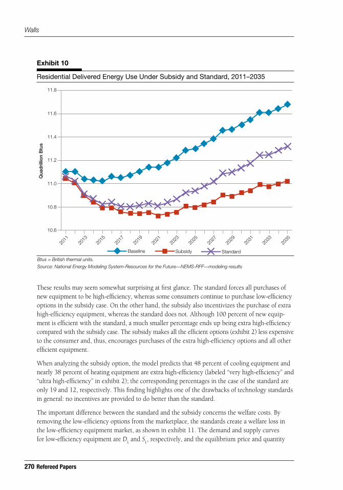
Exhibit 10 shows residential delivered energy use during the 2011-to-2035 period under the subsidy and the standard, with the baseline case shown for reference and the loan omitted for simplicity. The difference in energy use between the two policies is quite small. The standard has a smaller effect on energy use than does the subsidy, but cumulative residential delivered energy consump-tion during the 2011-to-2035 period is only 1.2 percent higher with the standard than with the subsidy. Cumulative economywide CO

2 emissions are nearly identical for the two policies. The

standard reduces CO2 emissions by 671.1 mmtons, compared with 672.5 mmtons for the subsidy.

Before 2027, the standard reduces CO2 emissions by slightly more than the subsidy in each year;

however, this outcome is reversed in the latter part of the forecast period, from 2027 to 2035. As a result, overall cumulative CO

2 emissions are roughly the same.

16 This lack of adjustment in equipment prices is a potential limitation of the modeling framework. In reality, an increase in demand for the high-efficiency equipment, forced by removal of the lower efficiency options, could increase prices (although to what extent is unclear). These market movements are not captured in my framework.

270

Walls

Refereed Papers

These results may seem somewhat surprising at first glance. The standard forces all purchases of new equipment to be high-efficiency, whereas some consumers continue to purchase low-efficiency options in the subsidy case. On the other hand, the subsidy also incentivizes the purchase of extra high-efficiency equipment, whereas the standard does not. Although 100 percent of new equip-ment is efficient with the standard, a much smaller percentage ends up being extra high-efficiency compared with the subsidy case. The subsidy makes all the efficient options (exhibit 2) less expensive to the consumer and, thus, encourages purchases of the extra high-efficiency options and all other efficient equipment.

When analyzing the subsidy option, the model predicts that 48 percent of cooling equipment and nearly 38 percent of heating equipment are extra high-efficiency (labeled “very high-efficiency” and “ultra high-efficiency” in exhibit 2); the corresponding percentages in the case of the standard are only 19 and 12, respectively. This finding highlights one of the drawbacks of technology standards in general: no incentives are provided to do better than the standard.

The important difference between the standard and the subsidy concerns the welfare costs. By removing the low-efficiency options from the marketplace, the standards create a welfare loss in the low-efficiency equipment market, as shown in exhibit 11. The demand and supply curves for low-efficiency equipment are D

L and S

L, respectively, and the equilibrium price and quantity

80

60

40

20

5

2011

2013

2015

2017

2019

2021

2023

2025

2027

2029

2031

2033

2035

7 9 11 13 15 17 19 21 23 25

0

– 20

– 40

– 60

– 80

U.S

. do

llars

per

to

n, 2

009

11.8

11.6

11.4

11.2

11.0

10.8

10.6

Qua

dri

llio

n B

tus

Discount rate (percent)

Subsidy Loan

Baseline Subsidy Standard

Exhibit 10

Residential Delivered Energy Use Under Subsidy and Standard, 2011–2035




271Cityscape

of low-efficiency equipment in the baseline, no-policy case are P0, L

and Q0, L

.17 Mandating that all equipment have the efficiency levels of the high-efficiency equipment effectively removes the low- efficiency options from the marketplace, which leads to a welfare loss illustrated by the shaded triangle in exhibit 11. This welfare loss is a measure of the cost to the economy from shifting re - sources away from these low-efficiency equipment options to the high-efficiency equipment market.

Calculating this area is not straightforward as I do not know the price at which the demand for low-efficiency equipment drops to zero. I assume it is equal to the equilibrium price of high-efficiency equipment—in other words, if consumers can buy high-efficiency equipment for the price of low-efficiency equipment, then demand for the latter should fall to zero. In the NEMS framework, this drop to zero actually does not happen. The market shares specification in the residential module will keep some low-efficiency models in the market even if their prices increase to more than the price of higher efficiency equipment. In this sense, my estimates understate the welfare costs. On the other hand, one would expect the price at which low-efficiency equipment demand falls to zero to be more than the high-efficiency equipment price because the latter options have lower energy costs. I simply point out the great deal of uncertainty in this reservation price and thus in my welfare cost calculations.

DL = demand curve for low-efficiency equipment. P = price of low-efficiency equipment purchased. P0, L and Q0, L = equilibrium price and quantity without standard. Q = quantity of low-efficiency equipment purchased. SL = supply curve for low-efficiency equipment. Shaded triangle = welfare loss from standard.

P

P0, L SL

D L

0 Q 0, L Q

Exhibit 11

Welfare Loss From Efficiency Standard

17 For ease of graphical exposition, I show a single market for low-efficiency equipment (as I did for high-efficiency equipment previously), but the NEMS-RFF model contains multiple equipment types.

272

Walls

Refereed Papers

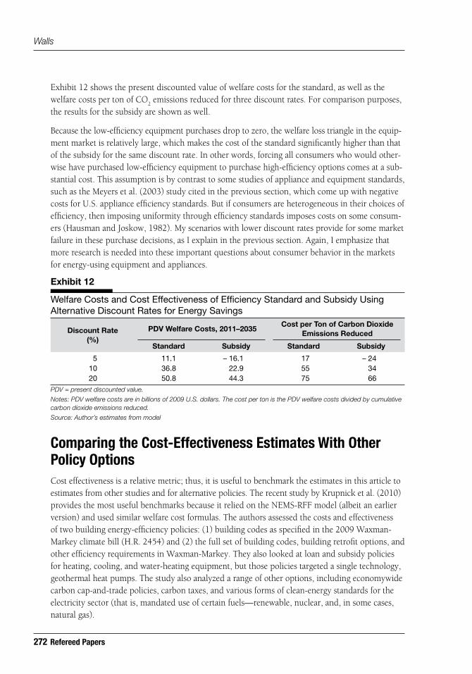
Exhibit 12 shows the present discounted value of welfare costs for the standard, as well as the welfare costs per ton of CO

2 emissions reduced for three discount rates. For comparison purposes,

the results for the subsidy are shown as well.

Because the low-efficiency equipment purchases drop to zero, the welfare loss triangle in the equip - ment market is relatively large, which makes the cost of the standard significantly higher than that of the subsidy for the same discount rate. In other words, forcing all consumers who would other - wise have purchased low-efficiency equipment to purchase high-efficiency options comes at a sub-stantial cost. This assumption is by contrast to some studies of appliance and equipment standards, such as the Meyers et al. (2003) study cited in the previous section, which come up with negative costs for U.S. appliance efficiency standards. But if consumers are heterogeneous in their choices of efficiency, then imposing uniformity through efficiency standards imposes costs on some consum-ers (Hausman and Joskow, 1982). My scenarios with lower discount rates provide for some market failure in these purchase decisions, as I explain in the previous section. Again, I emphasize that more research is needed into these important questions about consumer behavior in the markets for energy-using equipment and appliances.

Exhibit 12

Discount Rate (%)

PDV Welfare Costs, 2011–2035Cost per Ton of Carbon Dioxide

Emissions Reduced

Standard Subsidy Standard Subsidy

Welfare Costs and Cost Effectiveness of Efficiency Standard and Subsidy Using Alternative Discount Rates for Energy Savings

5 11.1 – 16.1 17 – 2410 36.8 22.9 55 3420 50.8 44.3 75 66

PDV = present discounted value.

Notes: PDV welfare costs are in billions of 2009 U.S. dollars. The cost per ton is the PDV welfare costs divided by cumulative carbon dioxide emissions reduced.

Source: Author’s estimates from model

Comparing the Cost-Effectiveness Estimates With Other Policy OptionsCost effectiveness is a relative metric; thus, it is useful to benchmark the estimates in this article to estimates from other studies and for alternative policies. The recent study by Krupnick et al. (2010) provides the most useful benchmarks because it relied on the NEMS-RFF model (albeit an earlier version) and used similar welfare cost formulas. The authors assessed the costs and effectiveness of two building energy-efficiency policies: (1) building codes as specified in the 2009 Waxman-Markey climate bill (H.R. 2454) and (2) the full set of building codes, building retrofit options, and other efficiency requirements in Waxman-Markey. They also looked at loan and subsidy policies for heating, cooling, and water-heating equipment, but those policies targeted a single technology, geothermal heat pumps. The study also analyzed a range of other options, including economywide carbon cap-and-trade policies, carbon taxes, and various forms of clean-energy standards for the electricity sector (that is, mandated use of certain fuels—renewable, nuclear, and, in some cases, natural gas).


273Cityscape

The Waxman-Markey building codes provision called for a 30-percent reduction in energy use in new buildings upon enactment of the law, a 50-percent reduction for residential buildings by 2014 and for commercial buildings by 2015, and a 5-percent reduction at 3-year intervals thereafter up until 2029 (residential) and 2030 (commercial). The retrofit provision required the U.S. Environ-mental Protection Agency to develop building retrofit policies to achieve the utmost cost-effective energy-efficiency improvements; the programs were to be administered through the states, which would receive CO

2 emissions allowances under the cap-and-trade program in H.R. 2454 to help

finance the programs. The bill also contained lighting provisions that created new standards for outdoor lighting, portable light fixtures, and incandescent reflector lamps and some provisions covering institutional appliances.

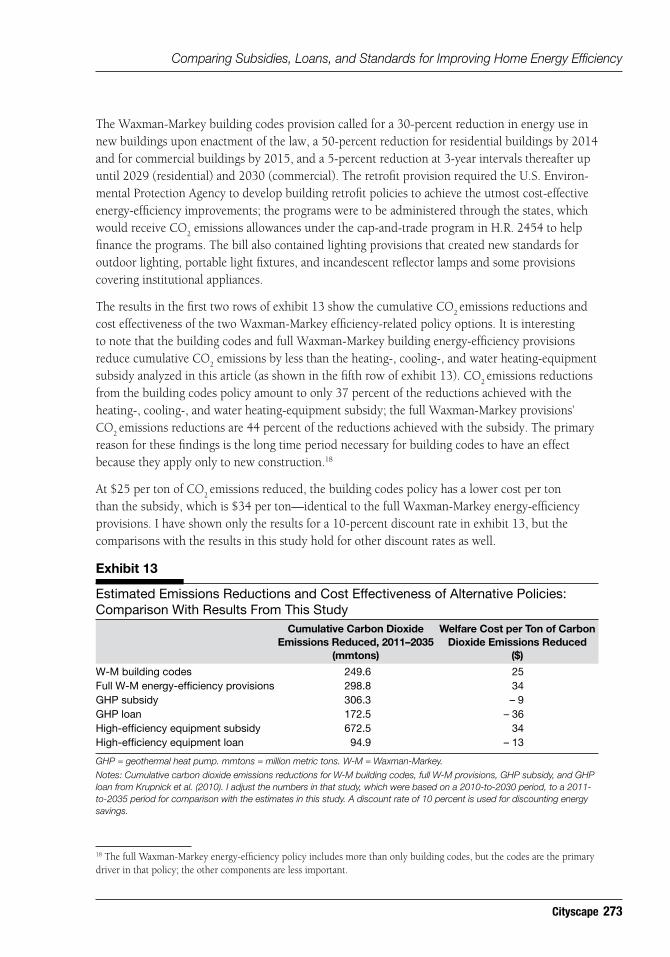
The results in the first two rows of exhibit 13 show the cumulative CO2 emissions reductions and

cost effectiveness of the two Waxman-Markey efficiency-related policy options. It is interesting to note that the building codes and full Waxman-Markey building energy-efficiency provisions reduce cumulative CO

2 emissions by less than the heating-, cooling-, and water heating-equipment

subsidy analyzed in this article (as shown in the fifth row of exhibit 13). CO2 emissions reductions

from the building codes policy amount to only 37 percent of the reductions achieved with the heating-, cooling-, and water heating-equipment subsidy; the full Waxman-Markey provisions’ CO

2 emissions reductions are 44 percent of the reductions achieved with the subsidy. The primary

reason for these findings is the long time period necessary for building codes to have an effect because they apply only to new construction.18

At $25 per ton of CO2 emissions reduced, the building codes policy has a lower cost per ton

than the subsidy, which is $34 per ton—identical to the full Waxman-Markey energy-efficiency provisions. I have shown only the results for a 10-percent discount rate in exhibit 13, but the comparisons with the results in this study hold for other discount rates as well.

18 The full Waxman-Markey energy-efficiency policy includes more than only building codes, but the codes are the primary driver in that policy; the other components are less important.

Exhibit 13

Cumulative Carbon Dioxide Emissions Reduced, 2011–2035

(mmtons)

Welfare Cost per Ton of Carbon Dioxide Emissions Reduced

($)

Estimated Emissions Reductions and Cost Effectiveness of Alternative Policies: Comparison With Results From This Study

W-M building codes 249.6 25Full W-M energy-efficiency provisions 298.8 34GHP subsidy 306.3 – 9GHP loan 172.5 – 36High-efficiency equipment subsidy 672.5 34High-efficiency equipment loan 94.9 – 13

GHP = geothermal heat pump. mmtons = million metric tons. W-M = Waxman-Markey.

Notes: Cumulative carbon dioxide emissions reductions for W-M building codes, full W-M provisions, GHP subsidy, and GHP loan from Krupnick et al. (2010). I adjust the numbers in that study, which were based on a 2010-to-2030 period, to a 2011-to-2035 period for comparison with the estimates in this study. A discount rate of 10 percent is used for discounting energy savings.

274

Walls

Refereed Papers

Rows 3 and 4 of exhibit 13 show the results for the GHP subsidy and loan policies analyzed in Krupnick et al. (2010). It is interesting to note the GHP subsidy is more cost effective at reducing CO

2 emissions than the broader equipment subsidy I analyze in this article, and likewise, the

GHP loan is more cost effective than my broader loan policy. These findings suggest that targeting subsidies and loans to very high-efficiency options—of which GHPs are one option—might be a more cost-effective approach. The GHP subsidy achieves smaller CO

2 emissions reductions than

the broader subsidy policy, but the GHP loan achieves slightly larger reductions.19

Compared with the other policy options analyzed by Krupnick et al. (2010)—particularly the econ - omywide cap-and-trade policies and the various types of clean-energy standards in the electricity sector—these building energy-efficiency policies are much less effective at reducing emissions and, except for the loan policy, less cost effective as well. The cap-and-trade policy, or an equivalent carbon tax, obviously is the most cost-effective instrument and the policy that generates the biggest reduction in CO

2 emissions because it targets all sources of CO

2 emissions. In Krupnick et al. (2010),

the estimated cost per ton of CO2 emissions reduced for the cap-and-trade policy was $12. The

clean-energy standards evaluated in Krupnick et al. (2010) are the next best options. These stand - ards require electricity generators to use clean sources for a specific share of the electricity they produce. Krupnick et al. (2010) found that a policy that incentivizes all fuels except coal (renewables, nuclear, and natural gas) in inverse proportion to their carbon content provides the largest reduction in CO

2 emissions and does so at a cost per ton of $15, very close to that of the cap-and-trade policy.

Cumulative CO2 emissions reductions for both policies are several times what can be achieved with

the energy-efficiency policies evaluated in this article.

Concluding RemarksEnergy experts have identified a number of improvement, upgrade, and retrofit options that homeowners can adopt to reduce their home’s energy use, and several of these changes seem to more than pay for themselves in the stream of energy savings they yield over time. Nonetheless, it has proved difficult to get homeowners to make these changes. One important barrier may be the upfront costs of new furnaces, additional insulation, more efficient windows and doors, upgraded appliances, and other options. In this study, I analyzed two policies to reduce the upfront cost of high-efficiency heating, cooling, and water-heating equipment—a direct subsidy and a zero-interest loan. Using the NEMS-RFF energy-market simulation model, I found that a subsidy that reduces upfront costs by 50 percent would cause a substantial shift in purchases toward high-efficiency options: during the 2011-to-2035 forecast period, approximately one-half of all heating and cooling equipment purchases are predicted to be high-efficiency units versus only about 20 percent in the baseline case. By 2035, the residential delivered energy-use forecast is 5.6 percent less than the baseline; on a per-household basis, the reduction is much larger, approximately 21 percent. Because residential buildings account for only about one-fifth of total CO

2 emissions in

the economy, however, economywide CO2 emissions during the 2011-to-2035 period are only 0.5

percent less than the baseline predictions for that period.

19 The subsidy and loan policies in Krupnick et al. (2010) are not exactly the same as the ones analyzed here. The GHP subsidy was $4,000 (more than the amount applied to GHPs here) and the loan was financed at 0 percent for 7 years, rather than the 3 years in this study.


275Cityscape

The welfare costs of the subsidy policy are fairly large: $34 per ton of CO2 emissions reduced when

future energy savings are discounted at a 10-percent annual rate. The cost estimate is highly sensi-tive to this discount rate, however: at 5 percent, the cost is negative—that is, the discounted stream of energy savings offsets the welfare loss from higher equipment costs—and, at 20 percent, the cost is as high as $66 per ton of CO

2 emissions reduced. Deciding which discount rate is the correct

one depends on one’s belief about the extent to which the efficiency gap, or energy paradox, is due to market failures. My 10-percent discount rate provides for the possibility of some market failure because that rate is higher than the 5-percent social discount rate but lower than the 20-percent rate in NEMS-RFF that reflects actual consumer behavior. More research is needed, however, into reasons for the energy paradox and how to discount costs and benefits.

The welfare costs are much lower for an energy-efficiency loan policy. I analyzed an option that reduces the upfront cost by 50 percent, exactly like the subsidy, but consumers must pay this money back during a 3-year period at a 0-percent interest rate. Estimated welfare costs for this policy option are -$13 per ton of CO

2 emissions reduced at a 10-percent discount rate, less than

-$100 at 5 percent, and +$42 at 20 percent. The negative costs mean that the discounted stream of energy savings offsets the welfare loss from higher upfront equipment costs. The loan policy does not make a noticeable dent in energy consumption and CO

2 emissions, how ever: the reduction is

one-tenth of the reduction that the subsidy accomplishes. Nonetheless, these results suggest that energy-efficiency-financing programs could be very cost effective. In reality, such programs have not accomplished much thus far (Palmer, Walls, and Gerarden, 2012), but it is possible that a large-scale national program could provide some CO

2 emissions reductions at relatively low cost.

I compared these incentive-based approaches with a command-and-control option—an efficiency standard applied to heating, cooling, and water-heating equipment. The specific policy I analyzed removes the low-efficiency options from the marketplace, thus all consumers are forced to buy high-efficiency equipment (that is, equipment that is at least as efficient as current ENERGY STAR models). This option reduces CO

2 emissions by about the same amount as the subsidy but at a

much higher cost. The welfare costs of a standard are higher because all consumers who purchase low-efficiency options in the baseline must now buy high-efficiency equipment at a higher price. I estimate that CO

2 emissions are reduced at a cost of $55 per ton when the discount rate is 10

percent, more than $20 higher than the cost of the subsidy.

The strength of the NEMS modeling framework is that it is benchmarked to national EIA forecasts and is continuously modified and updated to reflect current market and policy conditions. It captures economic behavior to some extent, thus one can see the incentive effects of policies that change effective prices. Moreover, by using a consistent modeling framework, an apples-to-apples com-parison of the three policies is possible. But like any simulation model, NEMS is not perfect. Some experts have criticized it for being conservative in its forecasts—that is, the responsiveness to policies is less than some believe is realistic. If NEMS should turn out to be excessively conservative, the es-timated CO

2 emissions reductions in this study may be biased downward. In addition, because of its

complexity, it is difficult to know what features of the model are central to the results one obtains. The model is costly to run, thus it is virtually impossible to run it under alternative assump tions to conduct sensitivity analyses on key parameters. Finally, my loan and subsidy policies targeted only

276

Walls

Refereed Papers

heating, cooling, and water-heating equipment; thus, the results do not necessarily carry over to other equipment or to whole-house retrofit options. A whole-house retrofit loan or subsidy policy would be difficult to model precisely in NEMS.

The findings about the relative effectiveness and cost effectiveness of the loan, subsidy, and stan-dard policy options are useful for providing a starting point for further discussions. In the absence of an economywide carbon tax or cap-and-trade policy, policymakers may be searching for options to deal with individual energy-using sectors one at a time. Improving the efficiency of residential and commercial buildings should be high on the list because these sectors account for more than 40 percent of current energy use, and many experts have identified a number of examples of low-hanging fruit in the building sectors. The retrofit problem, however, remains a challenging one. Further analysis is needed through modeling, case studies, and empirical-econometric studies to identify the most cost-effective and effective options for spurring building owners to adopt energy-saving retrofits and improvements.

Acknowledgments

The author thanks Todd Gerarden, Alan Krupnick, and Karen Palmer for their helpful comments on an earlier draft of this article. She also acknowledges the assistance of Frances Wood of OnLocation, Inc., in defining the policy scenarios and running the National Energy Modeling System—NEMS—model. The author also gratefully acknowledges funding from the S. D. Bechtel, Jr. Foundation.

Author

Margaret Walls is a research director and senior fellow at Resources for the Future.

References

Allcott, Hunt, and Michael Greenstone. 2012. “Is There an Energy Efficiency Gap?” Journal of Economic Perspectives 26 (1): 3–28.

Brown, Marilyn, Jess Chandler, Melissa Lapsa, and Moonis Ally. 2009. Making Homes Part of the Climate Solution: Policy Options To Promote Energy Efficiency. Oak Ridge, TN: Oak Ridge National Laboratory.

Browning, Edgar. 1976. “The Marginal Cost of Public Funds,” Journal of Political Economy 84 (2): 283–298.

Cowen, Tyler. 2008. “Social Discount Rate.” In New Palgrave Dictionary of Economics, 2nd ed., edited by Steven N. Durlauf and Lawrence E. Blume. Basingstoke, United Kingdom: Palgrave Macmillan.

Executive Office of the President. 2013. The President’s Climate Action Plan. Washington, DC: The White House. Also available at http://www.whitehouse.gov/sites/default/files/image/president27sclimateactionplan.pdf.

http://www.whitehouse.gov/sites/default/files/image/president27sclimateactionplan.pdf

http://www.whitehouse.gov/sites/default/files/image/president27sclimateactionplan.pdf


277Cityscape

Gillingham, Kenneth, Richard Newell, and Karen Palmer. 2009. “Energy Efficiency Economics and Policy,” Annual Review of Resource Economics 1: 597–619.

Gold, Rachel, Steve Nadel, John A. “Skip” Laitner, and Andrew DeLaski. 2011. Appliance and Equipment Efficiency Standards: A Money-Maker and Job-Creator. Report No. ASAP-8/ACEEE-A111. Washington, DC: American Council for an Energy Efficient Economy.

Harberger, Arnold C. 1971. “Three Basic Postulates for Applied Welfare Economics: An Interpre-tive Essay,” Journal of Economic Literature 9 (3): 785–797.

———. 1964. “The Measurement of Waste,” American Economic Review Papers and Proceedings 54: 58–76.

Hausman, Jerry, and Paul Joskow. 1982. “Evaluating the Costs and Benefits of Appliance Efficiency Standards,” American Economic Review 72: 220–225.

Hayes, Sara, Steven Nadel, Chris Granda, and Kathryn Hottel. 2011. What Have We Learned From Energy Efficiency Financing Programs? Report No. U115. Washington, DC: American Council for an Energy Efficient Economy.

Hines, James R., Jr. 1999. “Three Sides of Harberger Triangles,” The Journal of Economic Perspectives 13 (2): 167–188.

Hinkle, Bob, and Steve Schiller. 2009. New Business Models for Energy Efficiency. San Francisco, CA: CalCEF Innovations. Also available at http://calcef.org/files/20090301_Hinkle.pdf.

Jaffe, Adam, and Robert Stavins. 1994. “The Energy Paradox and the Diffusion of Conservation Technology,” Resources and Energy Economics 16: 91–122.

Just, Richard, Darrell Hueth, and Andrew Schmitz. 2004. The Welfare Economics of Public Policy. Northampton, MA: Edward Elgar.

Krupnick, Alan, Ian Parry, Margaret Walls, Tony Knowles, and Kristin Hayes. 2010. Toward a New National Energy Policy: Assessing the Options. Washington, DC: Resources for the Future.

McKinsey & Company. 2009. Unlocking Energy Efficiency in the U.S. Economy. New York; London, United Kingdom: McKinsey & Company.

Meyers, Stephen, James E. McMahon, Michael McNeil, and Xiaomin Liu. 2003. “Impacts of U.S. Federal Energy Efficiency Standards for Residential Appliances,” Energy 28: 755–767.

Mignone, Bryan, Thomas Alfstad, Aaron Bergman, Kenneth Dubin, Richard Duke, Paul Friley, Andrew Martinez, Matthew Mowers, Karen Palmer, Anthony Paul, Sharon Showalter, Daniel Steinberg, Matt Woerman, and Frances Wood. 2012. “Cost-Effectiveness and Economic Incidence of a Clean Energy Standard,” Economics of Energy and Environmental Policy 1 (3): 59–86.

National Academy of Sciences (NAS). 2010. Real Prospects for Energy Efficiency in the United States. Washington, DC: The National Academies Press.

Palmer, Karen, Margaret Walls, and Todd Gerarden. 2012. Borrowing To Save Energy: An Assessment of Energy Efficiency Financing Programs. Washington, DC: Resources for the Future.

http://calcef.org/files/20090301_Hinkle.pdf

278

Walls

Refereed Papers

State Energy Efficiency Action Network. 2011. “Residential Energy Efficiency Financing: Credit, Motivations and Products.” Slide presentation. February 7.

U.S. Department of Energy, Energy Information Administration (DOE/EIA). 2011. 2011 Annual Energy Outlook. Washington, DC: U.S. Department of Energy, Energy Information Administration.

———. 2009a. The National Energy Modeling System: An Overview. Washington, DC: U.S. Department of Energy, Energy Information Administration. Also available at www.eia.gov/oiaf/aeo/overview.

———. 2009b. Model Documentation Report: Residential Sector Demand Module of the National Energy Modeling System. Washington, DC: U.S. Department of Energy, Energy Information Administration, Office of Integrated Analysis and Forecasting.

______. 2009c. Energy Market and Economic Impacts of H.R. 2454, the American Clean Energy and Security Act of 2009. Washington, DC: U.S. Department of Energy, Energy Information Administra-tion, Office of Integrated Analysis and Forecasting.

———. 2008. 2005 Residential Energy Consumption Survey (RECS): Housing Unit Characteristics and Energy Usage Indicators. Washington, DC: U.S. Department of Energy, Energy Information Administration.

http://www.eia.gov/oiaf/aeo/overview

comparing subsidies, loans, and standards for improving

Documents