comparing rubber modified asphalt to conventional...
TRANSCRIPT

Department of Civil and Environmental Engineering Division of GeoEngineering Research Group Road and Traffic CHALMERS UNIVERSITY OF TECHNOLOGY Gothenburg, Sweden 2015 Master’s Thesis 2015:33
Comparing rubber modified asphalt to conventional asphalt Assessment of Trafikverket’s road survey tool Master’s Thesis in the Master’s Programme Infrastructure and Environmental Engineering
SANDRA HELLWIG ABDULLAH KARRI

MASTER’S THESIS 2015:33
Comparing rubber modified asphalt to conventional
asphalt
Assessment of Trafikverket’s road survey tool
Master’s Thesis in the Master’s Programme Infrastructure and Environmental
Engineering
SANDRA HELLWIG
ABDULLAH KARRI
Department of Civil and Environmental Engineering
Division of GeoEngineering
Research Group Road and Traffic
CHALMERS UNIVERSITY OF TECHNOLOGY
Göteborg, Sweden 2015


Comparing rubber modified asphalt to conventional asphalt
Assessment of Trafikverket’s road survey tool
Master’s Thesis in the Master’s Programme Infrastructure and Environmental
Engineering
SANDRA HELLWIG
ABDULLAH KARRI
© Sandra Hellwig & Abdullah Karri, 2015
Examensarbete 2015:33/ Institutionen för bygg- och miljöteknik,
Chalmers tekniska högskola 2015
Department of Civil and Environmental Engineering
Division of GeoEngineering
Research Group Road and Traffic
Chalmers University of Technology
SE-412 96 Göteborg
Sweden
Telephone: + 46 (0)31-772 1000
Cover:
The way of rubber tyres to asphalt (HNA, 2012) (ecore Athletic, n.d.) (RuBind inc.,
n.d.)
Department of Civil and Environmental Engineering. Göteborg, Sweden, 2015


I
Comparing rubber modified asphalt to conventional asphalt
Assessment of Trafikverket’s road survey tool
Master’s thesis in the Master’s Programme Infrastructure and Environmental
Engineering
SANDRA HELLWIG
ABDULLAH KARRI
Department of Civil and Environmental Engineering
Division of GeoEngineering
Research Group Road and Traffic
Chalmers University of Technology
ABSTRACT
Asphalt is more than a black material that covers our roads. It is a complex material that
contains various aggregates, fillers, bituminous binders and additives and can be
produced with different modifications. One of the latest modifications is asphalt with
rubber crumbs from recycled tyres. According to studies from the USA, rubber
increases the road surface’s resistance against wearing, plastic deformation and cracks,
which provides a longer lifetime compared to conventional asphalt.
The aim was to analyse if rubber modified asphalt (RMA) also would have the same
benefits on Swedish roads, considering the different climate zones and the use of
studded tyres during the winter period. The quality of the road surfaces was determined
by the condition of texture and rut depths. The results were based on annual surface
measurements on roads within the same climate zone, similar paving date and traffic
volumes. The suitability of the Swedish road administration’s tool (PMSV3) for road
surveys was also to be assessed. Comparing the measurements from PMSV3 to more
accurate measurements determined the quality of the survey data.
The RMA was best suited in climate zone 1 with a longer lifetime on most of the
analysed roads. In climate zone 2 the results were not clear enough for a certain
conclusion and in climate zones 4 and 5 no clear results were obtained due to
insufficient measurements. In climate zone 3 no roads were analysed. The texture on
rubber modified asphalts was better on most of the analysed roads in the south of
Sweden. The suitability of PMSV3 as a survey tool was analysed by comparing the
measurements on the E4 in Uppsala and the principle road 47 in Falköping. The values
differed by ±7% in Uppsala and ±18% in Falköping.
To conclude from the results PMSV3 is suitable as a survey tool regarding accuracy
and cost, but needs further revision. The rubber modified asphalt contributes with better
texture and increased rut resistance especially in climate zone 1. It has a good potential
and needs further measurements for clearer results.
Key words: Rubber modified asphalt, RMA, GAP, polymer modified asphalt, PMSV3,
Objektsmätning, rutting, texture, MPD, ABS

II
Jämförelse av gummimodifierad asfalt med konventionell asfalt
Bedömning av Trafikverkets analysverktyg för vägbeläggningar
Examensarbete inom master programmet Infrastructure and Environmental
Engineering
SANDRA HELLWIG
ABDULLAH KARRI
Institutionen för bygg- och miljöteknik
Avdelningen för geologi och geoteknik
Forskargrupp Väg och trafik
Chalmers tekniska högskola
SAMMANFATTNING
Asfalt är mer än ett svart material som täcker våra vägar. Produktionsprocessen är
väldig komplex då asfalt består olika aggregat, filler, bituminösa bindemedel och
tillsatser som gör att många olika modifieringar kan tillämpas. En av de senaste
modifieringar är asfalt med gummigranulat från återvunna däck. Enligt amerikanska
studier ökar gummimodifierade asfaltbeläggningars motståndskraft mot slitage,
plastiska deformationer och sprickor som resulterar i en ökad livslängd jämfört med
vanlig asfalt.
Syftet var att analysera om gummimodifierad asfalt (RMA) har samma förmåner på de
svenska vägarna med tanke på att klimatet skiljer sig och att dubbdäck används under
vinterperioden. Vägbeläggningens tillstånd bedömdes utifrån textur och spårdjup som
analyserades från mätningar på vägar i samma klimatzon, likartad beläggningsdatum
och trafikflöden. I den andra delen av arbetet bedömdes hur lämpligt Trafikverkets
analysverktyg (PMSV3) är för mätningar på asfaltytans tillstånd. Bedömningen
byggdes på jämförelsen av PMSV3’s mätvärden med värden från mer avancerade
mätmetoder.
Enligt beräkningarna lämpar sig användningen av RMA bäst i klimatzon 1, där texturen
var bättre och livslängden var längre än vanlig asfalt. I klimatzon 2 var resultaten inte
entydiga för en slutgiltig slutsats och i klimatzon 4 och 5 var värdena otillräckliga föra
att få tydliga resultat. I klimatzon 3 analyserades inte någon sträcka. För att bedöma
lämpligheten för PMSV3 jämfördes mätvärdena för E4:an i Uppsala och riksväg 47 i
Falköping, där mätvärdena skilde sig med ±7% respektive ±18%.
Slutsatserna är att PMSV3 väl lämpar sig för bedömningen av asfaltytans tillstånd ur
noggrannhets- och kostnadssynpunkt. Gummiasfalt uppvisade potential för bättre textur
och ökad slitagemotstånd främst i klimatzon 1 och behöver ytterligare mätningar för
tydligare resultat.
Nyckelord: Gummimodifierad asfalt RMA, GAP, polymermodifierad asfalt, PMSV3,
objektsmätning, spårdjup, textur, MPD, ABS

CHALMERS Civil and Environmental Engineering, Master’s Thesis 2015:33 III
Contents 1 INTRODUCTION 1
1.1 Background 1
1.2 Problem 1
1.3 Aim and objectives 2
1.4 Limitations of the report 2
1.5 Methods 2
2 LITERATURE REVIEW 3
2.1 Asphalt types 3
2.1.1 Conventional Asphalt 3
2.1.2 Modified Asphalt 5
2.2 Production methods 8
2.2.1 Job Mix formula 8
2.2.2 Conventional process 10
2.2.3 Rubber modified process 11
2.2.4 KGOIII 12
2.3 Deformation types 13
2.3.1 Rutting 13
2.3.2 MPD - Mean Profile Depth 13
2.3.3 Bleeding 15
2.4 Testing methods 15
2.4.1 Laboratory tests for aggregates 15
2.4.2 Laboratory tests for bitumen 17
2.4.3 Laboratory tests for asphalt sample 17
2.4.4 Field tests 20
2.5 Trafikverket system 23
2.6 Road surveys 24
2.6.1 PMSV3 Road network measurement 24
2.6.2 Object measurement (Objektsmätning) 24
2.6.3 VTI 24
2.7 Requirements from Trafikverket and VTI 25
2.7.1 Aggregates 25
2.7.2 Deformations 26
3 METHOD 27
4 ANALYSIS AND VERIFICATION OF RESULTS FOR ASPHALT 28
4.1 Climate Zone 1 30
4.1.1 E4 Kropp- Hyllinge med 30
4.1.2 E6 Fredriksberg- Lockarp KF10 & 20 mot 34

CHALMERS, Civil and Environmental Engineering, Master’s Thesis 2015:33 IV
4.1.3 E6 Kronetorp- Salerup mot 37
4.1.4 E6 Petersborg- Vellinge KF10 & 20 mot 40
4.1.5 E6 Sunnanå- Kronetorp KF10 & 20 med 43
4.2 Climate Zone 2 45
4.2.1 E6 Ullevi- Kallebäck 45
4.2.2 RV47 Falköping med 48
4.2.3 E4 Uppsala-Knivsta 52
4.2.4 E4 Viby- Sollentuna (Stockholm) KF30 mot 59
4.3 Climate Zone 4 61
4.3.1 Västerbotten - E4 Broänge-Hökmark K10 61
4.4 Climate Zone 5 64
4.4.1 Västerbotten - E12 Lycksele K10 64
4.4.2 Västerbotten - E12 Storuman- Stensele K10 med 70
4.4.3 Norrbotten - E4 Gäddvik-Nickbyn K10 73
4.5 Result overview 79
5 DISCUSSION 81
6 CONCLUSIONS AND FUTURE RECOMMENDATIONS 87
7 REFERENCES 89
8 LIST OF FIGURES 93
9 LIST OF TABLES 98
10 LIST OF EQUATIONS 100
APPENDIX 101
Appendix I: E4 Kropp-Hyllinge 101
Appendix II: E6 Fredriksberg-Lockarp 105
Appendix III: E6 Kronetorp-Salerup 108
Appendix IV: E6 Petersborg-Vellinge 111
Appendix V: E6 Sunnanå-Kronetorp 114
Appendix VI: E6 Ullevi-Kallebäck 117
Appendix VII: RV47 Falköping 120
Appendix VIII: E4 Uppsala-Knivsta 121
Appendix IV: E4 Viby-Sollentuna (Stockholm) 124
Appendix X: E12 Lycksele 126
Appendix XI: E12 Storuman-Stensele 127
Appendix XII: E4 Gäddvik-Nickbyn 129
Appendix XIII 131

CHALMERS Civil and Environmental Engineering, Master’s Thesis 2015:33 V
Preface
We are proud to have finished our education in Civil Engineering with a Master’s in
Infrastructural and Environmental Engineering with this thesis.
This thesis is an attempt to support the Swedish transport administration with its
maintenance work on asphalt pavements. It had also the goal to be part of the rubber
asphalt development that currently is going on in Sweden. Our role in this development
was to analyze the current state of the performance of rubber asphalt test sections in
Swedish climate conditions and provide a base for future analyses and working
procedure. All conclusions made in this report are our own and were based on the results
and experience we have gathered during our work.
We want to thank our supervisors Jan Englund at Skanska and Torsten Nordgren at the
Swedish transport administration for making this thesis possible and for the support and
material they have provided during our work. We would also like to thank our
supervisor and examiner Gunnar Lannér at Chalmers University of Technology for his
help and advice.
Finally we want to thank all the people that have answered our questions, contributed
with ideas and showed interest for our work.
June 2015
Sandra Hellwig and Abdullah Karri

CHALMERS, Civil and Environmental Engineering, Master’s Thesis 2015:33 VI
Notations
ABS Asphalt concrete, high percentage of stones, standard type
ABT Asphalt concrete, dense
B Bituminous binder (bitumen)
GAP Dense rubber modified asphalt
GMB Rubber modified bitumen
HABT Asphalt concrete, hard and dense
IRI International roughness index
KF10 First lane from the right
KF20 Second lane from the right
KF30 Third lane from the right
KGOIII Karl Gunnar Olsson asphalt mixing method
Med Driving direction, south to north, west to east
Mot Driving direction, north to south, east to west
MPD Mean profile depth, describes the texture of the road surface
measured in mm
MPD left MPD on the left side of the lane
MPD middle MPD on the middle part of the lane
MPD right MPD on the right side of the lane
Objektsmätning Special measurement for a road test section under regulated
conditions
PMB Polymer modified bitumen
PMSV3 Pavement Management System volume 3, Trafikverket’s
database for road data
RMA Rubber modified asphalt
Rubber crumbs Product from used car and truck tires used in RMA
Rutting, rut depth Vertical compression or wearing of asphalt caused by tires,
measured in mm
Rutting max 15 Rutting measured with maximum 15 lasers on the measuring car
RV Riksväg, principal road
Trafikverket Swedish Transport Administration
VTI State road- and transport research institution
ÅDT Total annual traffic divided on one day, vehicles per day

CHALMERS Civil and Environmental Engineering, Master’s Thesis 2015:33 VII

CHALMERS, Civil and Environmental Engineering, Master’s Thesis 2015:33 VIII

CHALMERS Civil and Environmental Engineering, Master’s Thesis 2015:33 1
1 Introduction
1.1 Background
For a country the road network is as vital as the veins for the human body. All forms of
transport, whether it is public transport, goods or car traffic rely on roads that provide
safety, comfort and mobility. Since most of the roads are paved with asphalt, this
material has a crucial effect on the driving quality and can be influenced in many
different ways, ranging from the production process to material composition (Nordgren,
2015).
Asphalt has been used for a very long time as a sealer and construction material and
could be tracked back to 3200 BC. The first modern use of this material occurred in
1829 in Lyon as a road surface for walkways. In Sweden asphalt was introduced in
Stockholm for the very first time in 1876 at Stora Nygatan (Asfaltskolan, n.d.).
Even though asphalt is a very resistive material it can offer high performance under a
limited time and tolerate loads to a certain degree. If lifetime or bearing capacity are
exceeded, wearing appears in different forms and sizes. The most common
deformations are rutting, decreased skid resistance and surface cracks. Typical causes
include high axle loads (trucks), extreme temperature alterations or wrong material
composition. In order to prevent these kinds of damages or to minimise the extent of
their impact on the asphalt, several modifications have been developed in the material
composition, material properties and in the production process. Today there are many
different asphalt types optimized for different purposes and areas of use. More details
and asphalt properties will be described further on in the project.
1.2 Problem
The Swedish transport administration (Trafikverket) is responsible for maintaining the
public road network in order to provide safe, fast and comfortable every day driving.
With annual surveys the road condition is controlled and investigated for any kind of
damage. All data that is collected during these surveys is stored in a system called
Pavement Management System (PMSV3), which is the Swedish transport
administration’s main tool for assessing the current road surface condition and is
available as open source.
The VTI survey is a special ordered road survey using more advanced techniques and
equipment. Roads are closed down for public traffic during these surveys in order to
avoid any outer disturbance for the best possible results. Typical areas of use for VTI
surveys are surface property analysis for new asphalt types, asphalt modifications and
their comparison with standard asphalt. Another survey used is an object measurement
(Objektsmätning), which uses the average value of three measurements for the same
road section.
A new asphalt type that recently has been tested on Swedish roads is rubber modified
asphalt. Many test tracks were constructed all around Sweden to determine if rubber
modified asphalts are suitable for the country’s roads and climate and if they result in
longer lifetime, better surface properties and less wearing and deformation.

CHALMERS, Civil and Environmental Engineering, Master’s Thesis 2015:33 2
For this project the focus will be on the questions mentioned below.
1. Is PMSV3 convenient for road surveys?
2. Is rubber modified asphalt more resistant than conventional asphalt regarding
rutting and change in texture over time?
3. Is rubber modified asphalt more profitable from a long term perspective?
1.3 Aim and objectives
The aim with this project consists of two parts. The first part is the comparison of rubber
modified asphalt to conventional asphalt from a life time perspective. The second part
is the suitability assessment of PMSV3 as an analytical tool
1.4 Limitations of the report
Trafikverket judges the road condition by four aspects, which are rutting, texture, IRI
and deformation of the road edge. The comparison of the asphalt types and the
analytical tools will be limited to two parameters, namely rutting and texture as well as
to Swedish roads. Other deformations will be excluded in the results section. Moreover,
the focus will be on rubber modified asphalt and standard asphalt despite other asphalt
types appearing in the report.
1.5 Methods
Literature will be the base for the theoretical background of the project to gain
understanding for the different asphalt types, production processes as well as
deformations and how these are measured.
In order to establish the comparison of rubber modified asphalt to standard asphalt
following steps will be used:
Gather data from PMSV3
Sort the data by date of placement, asphalt type and traffic volumes
Calculate average rut depth and texture for each year and asphalt type
Calculate the annual increase/ decrease for rut depths and texture for each type
After these steps the results will be presented in diagrams which enable a direct
comparison. Furthermore, the results will be controlled if they fulfil Trafikverket’s and
VTI’s requirements regarding rut depth and texture, as well as the remaining time
before maintenance based on the latest measurement and average annual increase in rut
depth.
PMSV3’s suitability as an analysis tool will be assessed by comparing the rut depths
measured by PMSV3 to Objektsmätning and VTI.

CHALMERS Civil and Environmental Engineering, Master’s Thesis 2015:33 3
2 Literature review
In this chapter information about different asphalt types and production processes will
be provided. The information has been retrieved from technical books, reports, studies
and from the internet. Moreover, the testing methods and deformation types will be
presented as a support to aid the understanding of the results in further chapters.
2.1 Asphalt types
Each asphalt type has a special purpose, area of use or specifications, which can be
influenced in many ways during the production process. Most of the asphalt properties
rely on the gradation, which is the aggregate size distribution, as well as the bitumen
quality.
2.1.1 Conventional Asphalt
Asphalt is composed of the three main ingredients, aggregates, fillers and a binder
(Bitumen). Air voids are also present in the mass depending on the grade of compaction.
Other additives, such as cement occur also as ingredients. The mixture influences the
quality and life time of the pavement (O'Flaherty, 2002).
Aggregates
Aggregates are crushed hard stones of different fractions. The main requirements for
aggregates are the particle size distribution curve, the flakiness index and Ball-Mill
value (Parhamifar, 2014). Aggregates are the most important part within an asphalt
concrete surface to provide the essential resistance to the load and wearing. That is the
reason why aggregates are present in a high amount in the asphalt concrete pavement.
Figure 1: Different sizes of aggregates (Werner Corporation, n.d.)
They can be classified in different ways either by their origin or type of preparation. Pit
or bank aggregates are natural aggregates, which only need to be screened to the desired
size and washed before using for asphalt production. Processed aggregates on the other
hand are also natural stones, however they need to be blasted, crushed and screened to
an accurate size, see Figure 1. The crushing process enables to shape the particles to an
accurate size range. Another type of aggregates is synthetic, which are produced by
changing the properties of the stone material (APAI, n.d.). This is either done to
produce aggregates or can be a by-product.

CHALMERS, Civil and Environmental Engineering, Master’s Thesis 2015:33 4
Furthermore, aggregates can have different properties beside size and shape, such as
roundness, surface texture, hardness and absorption.
Trafikverket has requirements concerning aggregates, which are closer described in
Chapter 2.7.1.
Bitumen
The key ingredient of the asphalt mixture is bitumen (binding material). It is a bi-
product from the oil production and is necessary to keep the aggregates attached to each
other, see Figure 2. Additional functions of the bitumen are to prevent the aggregates
from crushing, giving it strength to shape itself without failing, as well as giving the
asphalt its bearing capacity (Parhamifar, 2014).
Figure 2: Aggregates covered in bitumen (Petro Asian FZC, n.d)
The properties of bitumen depend on the crude oil properties which vary with the origin.
One property is viscosity, which relies on temperature; at high temperature bitumen is
liquid and becomes solid at a low temperature (Persson, 2014). The most common
process is the refining of crude oil with atmospheric and vacuum distillation. Here
lighter fractions, liquid petroleum gas, are separated first in atmospheric distillation and
remaining fractions are removed within the vacuum distillation. The last step is done to
prevent overheating. Further processes are available to achieve a variety of different
properties (Persson, 2014).
To obtain the main properties of the bitumen different test are available, the softening
point test, also called ring and ball method, and the needle penetration rate test, further
described in Chapter 2.4.2.
In colder climate a softer binder shall be used due to its properties, and harder binder in
warmer climate. In order to choose the correct binder type it is necessary to know the
different climate zones in Sweden and in which one the asphalt will be used, see Chapter
4.
The price of bitumen is related to the price of HSFO, refining High Sulphur Fuel Oil;
and additional costs of production, storage, packaging and additives.

CHALMERS Civil and Environmental Engineering, Master’s Thesis 2015:33 5
2.1.2 Modified Asphalt
Changing demands on roads, pavements and additional climate changes have made it
necessary to look deeper into the asphalt properties. The aim was to modify bitumen
and asphalt so that the properties fulfil the higher demands and can meet these changes.
One solution was additives, which are added to the bitumen or to the final asphalt mix.
Below two different types of modification are described.
Polymer Modified Asphalt
Due to an increasing traffic load and a rapidly changing climate new kinds of asphalt
need to be developed to resist these changes. One solution is to add polymers to either
asphalt or bitumen (Persson, 2014).
These modifications were firstly patented during the mid-19th century with natural and
synthetic polymers, mainly using neoprene latex and during subsequent-centuries the
modification was further developed. Therefore in the 1970s PMA was commonly used
in Europe due to lower maintenance cost, however further development of polymers
made it more attractive to use in the US and other parts of the world (Yildirim, 2005).
The most common polymers that are styrene-butadiene rubber (SBR), styrene-
butadiene – styrene (SBS), ethylene-vinyl-acetate (EVA), polyethylene and rubber
(Yildirim, 2005).
This modification can increase the resistance of the pavement to withstand the
increasing traffic load (Persson, 2014). Additionally, the main aim of PMA is to achieve
greater elastic recovery of the binder, a higher softening point and viscosity as well as
improving the cohesive strength and ductility when compared to conventional asphalt
(Yildirim, 2005).
Rubber modified asphalt (RMA)
The modification of bitumen with rubber started in the early 1840’s in the USA with
the purpose to develop a road surface treatment with higher elasticity. The goal was to
enhance the elastic properties of the binder through the addition of natural (latex) and
synthetic rubber (crude oil based polymers). Since then, on-going development had
continued until the early 1960s, when Charles McDonald, materials engineer for the
City of Phoenix, succeeded in creating an asphalt mix with rubber crumbs.
Sweden also performed some tests in the 1950s with the goal of improving the road
surface properties in addition to solving the environmental issue with scrapped tires
(Asfaltskolan, n.d). They came up with a technique later on, the dry process, which is
described later on in the report.
McDonald’s success initiated entire projects to test the new surface treatment,
whereupon many new asphalt products were developed such as Stress Absorbing
Membranes (SAM) and Stress Absorbing Membrane Interlayers (SAMI) (Heitzman,
1992). As illustrated in Figure 3, the SAM layer is a chip- seal coat using asphalt-rubber
instead of pure bitumen binders in the conventional method. When the SAM is overlaid
with a coat of hot mix asphalt it is referred to as SAMI (FHWA, 2012).

CHALMERS, Civil and Environmental Engineering, Master’s Thesis 2015:33 6
Figure 3: Schematic design SAM & SAMI (Way, George, 2012)
In the chip seal coating procedure the hot asphalt- rubber liquid is sprayed on the road
surface, followed by aggregate material. The hot liquid is sprayed with a special
distributor truck and the aggregates are spread out immediately and evened out with a
roller as illustrated in Figure 4 (Carlson & Zhu, 1999). This technique however is
mainly used in the US and not common in Europe, due to the bad working environment
including fumes (Nordgren, 2015).
Figure 4: Chip seal coating. Spreading out aggregates on hot asphalt- rubber liquid (City of Mankano, n.d)
The main functions of the layers with rubber modified asphalt are:
Absorption of stress caused by traffic and impact reduction on the remaining
road construction
Decrease reflective cracking
Decrease noise
Higher tolerance to thermal changes
Decrease overall costs
Better skid resistance
RMA’s are produced in two different processes, the wet process and the dry process
which give the asphalt different final performance- and working properties. These are
described in the coming chapters of this report.
Advantages
Studies in northern and central Arizona on asphalt-rubber mixes showed that these
modifications increase resistance against aging to a small degree. Moreover, increased
resistance to hardening and improved fatigue life has been indicated as well as
decreased sensitivity to temperature changes. The softening point for the asphalt-

CHALMERS Civil and Environmental Engineering, Master’s Thesis 2015:33 7
rubber increased by 11-14 °C, which is an important factor for rutting during warmer
periods of the year (FHWA, 2012). Another benefit is the increased skid resistance and
binder elasticity, which reduces the risk for rutting and cracking (Amirkhanian, 2013).
The greatest benefits of asphalt- rubber hot mix overlays were the reduced layer
thicknesses and the associated reduction in the material usage and maintenance costs.
Both chip seals and the hot mix overlays were found to have a great effect on reducing
the reflection of alligator cracks, however the hot mix overlay provided a better riding
surface and decreased traffic noise (FHWA, 2012). In general, RMA provides a longer
overall pavement life and the possibility to use standard HMA paving and compaction
equipment facilitates the work for contractors (Amirkhanian, 2013).
Disadvantages
Despite all benefits from RMA it also comes with some disadvantages. The use of RMA
implies higher initial costs, which were twice the price of conventional asphalt. When
the patents ended the price went down continuously and nowadays RMA costs 10-20
% more than conventional asphalt in the USA (Way, et al., 2011). Another drawback
is the need for a blending unit and an agitated binder storage tank, if terminal blending
is not used, which implies additional costs (Amirkhanian, 2013).
Not all contractors are familiar with the use of RMA, since the workability, binder
storage stability and the emission of fumes is different than conventional asphalt. In
addition to that it needs to be placed within a very short time, since the temperature
must not sink too much (Lo Presti, et al., 2012).
Costs for rubber modified asphalt
Asphalt types come with various properties and can be made in different qualities. The
choice of the asphalt type depends then on the cost. Rubber modified asphalt in Sweden
is in general 20 to 30% more expensive than conventional asphalt (Nordgren, 2015).
The additional costs emerge from the extra steps in the manufacturing process such as:
Cost for rubber crumbs
Complex manufacturing
Higher amount of bitumen
Lower production capacity for the mixing unit
For these reasons the modified asphalt layers need to provide longer lifetime in order
to compensate for the additional costs. How much longer it needs to last depends on the
designed lifetime and varies from road to road.

CHALMERS, Civil and Environmental Engineering, Master’s Thesis 2015:33 8
2.2 Production methods
The production process starts outside the factory. The requirements on the asphalt, such
as amount of traffic, axle loads and climate zone determine the choice of type and
amount of aggregates as well as binder. The next steps in the process occur in the
factory where the mixing begins.
There are a variety of production processes, each with advantages and disadvantages.
In the sections below the conventional process is presented in addition to a recently
applied process with the name KGOIII.
2.2.1 Job Mix formula
The job mix formula is the first step in the production and can be compared to a recipe,
where size and distribution of aggregates are determined in addition to the type and
amount of binder. As previously explained each component comes with special
properties, which are chosen according to the requirements for the new asphalt. Since
achieving a perfect mix is very hard, upper and lower gradation limits are set as a range
to keep the desired properties of an asphalt mix (Parhamifar, 2014).
Trafikverket has established guidelines and requirements on the material and asphalt to
make sure the least allowed quality is maintained. More details about guidelines are
available at Trafikverket’s website with the search word underhållsstandard.
Gradation of asphalt concrete mixes
Asphalt mixes are divided into different gradations, each to fulfil certain properties of
a road project or maintenance. The differences are shown in Figure 5.
Figure 5: Aggregate structure in dense-, gap- and open graded asphalts (Tariq, 2013)
Dense-graded
Dense graded asphalt contains a well proportioned mixture of bituminous binder,
aggregates, filler material, and/or some additives to change the final properties
(Queensland Government, 2009). In dense graded rubber asphalts the rubber content
varies between 5-10% by binder weight (Amirkhanian, 2013). It can be used in several
layers of the road body as an almost impermeable layer to let water run off the road
surface and improving the riding quality of the road, if used as a surface layer. The
drawbacks though, are its sensitivity to hot climate and temperature variations, which
could cause thermal cracking and a high risk of mirroring and less effective
retroflection. In Figure 6 below, an example of a dense- graded asphalt concrete mix
composition can be observed.

CHALMERS Civil and Environmental Engineering, Master’s Thesis 2015:33 9
Figure 6: Dense graded asphalt mix (Way, George, 2012)
Open-graded
Open graded asphalt is composed of bituminous binder, aggregates and filler with or
without additives (Queensland Government, 2009). It usually contains 12% to 20%
rubber of the total binder mass if rubber asphalt is mixed (Amirkhanian, 2013). Only
small amounts of fine material are used in order to achieve a high percentage of air
voids. Figure 7 clarifies the proportions in an open gradation, especially the high
content of larger aggregates. This type of asphalt is applied as a friction course with the
purpose to decrease noise, increase skid resistance and increase surface drainage for
higher safety.
Figure 7: Aggregate content in open graded asphalt mix (Way, George, 2012)
Gap-graded
The structural differences of the gradations are shown in Figure 5. Gap- graded asphalt
contains a large amount of coarse and fine aggregates, but a very small proportion of
medium- sized aggregates. It has performance properties similar to the dense-graded
asphalt mix; the difference though lies in the void distribution. The gap gradation
creates a few large voids, whereas the dense gradation creates many small voids
(Clemson University, 2002). In the rubber modified version the added amount of rubber
should range from 18-20% (Amirkhanian, 2013). This type of gradation has good
drainage for use in residential areas. Due to the porous structure more maintenance is
necessary during the life time.

CHALMERS, Civil and Environmental Engineering, Master’s Thesis 2015:33 10
2.2.2 Conventional process
The conventional hot asphalt mix production process consists of many steps in order to
reach the highest quality for the final product. In this process coarse and fine aggregates
are mixed together with mineral filler and finally bitumen as the binder. The optimal
proportion is obtained in a so called Job Mix Formula, which has specifications for each
aggregate size and binder content. Once the asphalt mix is processed the aggregates
contribute to 92% of the total weight (EPA, 1995).
There are many different hot mix asphalt plants such as Batch Mix Plants, Parallel Flow
Drum Mix Plants and Counter flow Drum Mix Plants that use different techniques for
asphalt production. To stay within the scope of this project, only the batch mix plant
will be described since it is the most common mixing plant in Europe (Nordgren, 2015).
In batch mix plants (Figure 8) the aggregates are placed in hoppers of the cold feed unit
and transported to a dryer. In the next step the aggregates have to pass vibrating screens
that separate the aggregates into different sizes. Afterwards the aggregates are stored,
according to their size, in heated containers. While the aggregates are weighed and
mixed according to the recipe, hot liquid bitumen is pumped into an asphalt bucket in
the proper aggregate bitumen ratio. The aggregates are then dropped into the mixer and
mixed for 6 to 10 seconds before the hot liquid bitumen is added and mixed with the
aggregates for usually less than 60 seconds. Finally the hot mixture is either stored in a
hot storage silo or dropped in a truck and transported to the job site (EPA, 1995).
Figure 8: Batch Mix Plant (EPG, 2007)

CHALMERS Civil and Environmental Engineering, Master’s Thesis 2015:33 11
2.2.3 Rubber modified process
For modified asphalt two mixing types exist; the wet and the dry process. Both are
explained further in the Chapters below.
Wet process
In Sweden the most common method for rubber modified bitumen is the wet process.
In the wet process, crumb rubber is used as a modifier for the bitumen. When the rubber
is added to the asphalt and blended together a reaction starts, during which the rubber
swells and softens. Continuous agitation (high viscosity process) is necessary in order
to keep a homogenous mass and avoid a non-uniform distribution of the rubber crumbs
in the mix (Lo Presti, et al., 2012). During the production of polymer modified bitumen
the same process is used (Nordgren, 2015).
This process is influenced by the temperature and time and even the components of the
materials used in the mix. The recommendations from the FHWA1 are to keep the
mixing temperature between 166˚C and 204˚C, and a reaction time between ten minutes
up to two hours. The amount of crumb rubber, which is added to the bitumen can range
from 18 to 25%.
According to the California Department of Transportation road overlays of a wet-
process are less sensitive to distress, deflections and require less maintenance compared
to conventional asphalt concrete (FHWA, 2012).
Another form of the wet- process is also known as the terminal blend or field- blend.
In the refinery, the bitumen and rubber crumbs are mixed together at higher shear stress
(up to 8000 revolutions per minute) at higher temperature (200 to 260˚C) until the
rubber crumbs are completely digested in the binder, by depolymerisation. The
difference between the two processes becomes clear in Figure 9. Terminal blend- binder
can then be delivered as a conventional binder to the asphalt plant, which can use it
without any modifications for the asphalt production (Lo Presti, et al., 2012).
Figure 9: Rubber modified bitumen- high viscosity (left) and terminal blend (right) (Lo Presti, et al., 2012)
Dry process
In the late 1970s the dry process was developed and patented under the name PlusRide
by EnviroTire. Here the granulated or crumbed rubber (1 to 3 weight percentage of the
total mix) is added as part of the fine aggregates, not part of the binder as it is in the wet
process. The size of the rubber particles varies from 2.0 mm to 4.2 mm. The difference
from conventional asphalt methods is that this process produces denser asphalt with a
void content of 2 to 4%, instead of 7.5 to 9%. Moreover, this process creates asphalt
1 Federal Highway Administration, USA
CHALMERS, Civil and Environmental Engineering, Master’s Thesis 2015:33 12
with higher binder content, usually 10 to 20% higher than conventional asphalt
(FHWA, 2012).
The addition of rubber requires both increased mixing time and temperature, which lies
between 149˚C to 177˚C including preheating of the aggregates and rubber crumbs. The
mixture is paved at 121˚C and needs continuous compacting until it decreases below
60˚C, otherwise the mixture would swell and be deformed (FHWA, 2012).
2.2.4 KGOIII
The KGOIII (named after its developer, Karl Gunnar Olsson) is a mixing process,
developed to increase the level of homogenisation in the asphalt mixture. This process
provides a thicker binder film (bitumen) and enables a complete coverage of the coarse
stone material compared to conventional mixing methods (Andersson, 2008).
The process needs to follow a certain order to reach the best possible consistency and
homogeneousness. First, the coarse ballast material (larger than 4mm) and the bitumen
are added in the mixer followed by filler material, which is evenly spread in the mix.
Finally the smaller ballast components (0 to 4 mm) are added, hence allowing the filler
and the bitumen to distribute more evenly throughout the whole mass (Andersson,
2008).
Asphalt mixes for the KGOIII process have to follow strict guidelines in order to meet
the standards for pavements. Compared to conventional processes the mixture in the
KGOIII process should have higher content of material larger than 4mm. In addition to
that the material passing through the 2 and 4 mm sieve must not exceed 8% and material
passing through the 4 and 8 mm sieve should maximum be 18% (Andersson, 2008).
Heat and temperature are crucial in the mixing process. The temperature should be kept
between 130°C and 140°C and temperatures over 150°C must be avoided in order to
prevent the asphalt mix from damaging (Andersson, 2008).
Advantages with KGOIII
The advantage with this method is to achieve a better and more complete coverage of
the stone material and a thicker bitumen film around them. This makes the asphalt more
resistant to wearing. Moreover the process requires lower temperatures and lower
binder content (0.5% less binder) without compromising compaction and pavement
properties, which enables saving energy and decreasing environmental impacts.
Disadvantages with KGOIII
This method has some drawbacks, however not in the quality. The drawbacks lie in the
production capacity of the asphalt plant and the workability of the mass. The longer
mixing processes lower the capacity of some asphalt plants, causing losses or forcing
them to extend the production facility in order to compromise the slowdown.
Another point is that the KGOIII asphalt is more sensitive to failures in the mixing
process and therefore requires careful management, as well as it is tougher to work with
than conventional asphalt. In the paving process also problems with joints, roller cracks
and fat parts (when temperature is too high) were indicated.

CHALMERS Civil and Environmental Engineering, Master’s Thesis 2015:33 13
2.3 Deformation types
A variety of deformations can appear due to external and internal influences, such as
traffic load, climate and the E-Moduli of the subgrade. These are also reasons for a
change in road surface properties and performance, which make it necessary to maintain
the roads on a regularly base.
2.3.1 Rutting
Rutting appears in form of surface depression or compression in wheel tracks. This can
be caused by deformations of any of the pavement layers or subgrade. This occurs either
as a result of bad compaction during construction or plastic movement during warmer
temperatures and high traffic loads, see Figure 10 (Huang, 2003). In Nordic countries
the use of studded tires is common, which also cause rutting by wearing out material
each time a vehicle passes over the surface (Nordgren, 2015).
This deformation is especially visible after heavy rains and known as hydroplaning,
which can be a high risk for car drivers.
Figure 10: Extreme rutting in wheel paths (Auto Vina, 2012)
It can be measured as rut depth in mm with a dipstick every 15 meters or with help of
a photographic distress survey (Huang, 2003). Nowadays, the rut depth is measured
with either 15 or 17 lasers on a measurement car. The data for 17 lasers may be incorrect
when measuring on smaller roads, due to driving on the road side marking and
measuring from the wrong origin. There the measurement with 15 lasers is
recommended considering that the lanes in Sweden are getting more narrow (Nordgren,
2015).
Requirements from Trafikverket concerning rut depth are shown in Chapter 2.7.2.
2.3.2 MPD - Mean Profile Depth
The road surface is described in different forms of texture. In year 2005, Trafikverket
decided that the macro texture has to be measured by mean profile depth (MPD) as a
standard requirement. MPD is used internationally as a standardized measurement.
From 2010 the mega texture has to be measured as well in order to identify irregularities

CHALMERS, Civil and Environmental Engineering, Master’s Thesis 2015:33 14
such as potholes or bridge edges. Macro texture is supposed to measure the road
surface’s homogeneity for the distribution of aggregates and binder.
The surface texture has great influence on many road properties and affects friction,
intern- and extern noise emission, rolling resistance, tire wear, dewatering, drainage,
light reflection as well as possibly the generation of particles. Macro texture is
measured between 0.5 and 50 mm and affect properties as illustrated in Figure 11.
Figure 11: Micro-, macro-, and mega texture with respective wavelength interval as well as irregularities after
(Lundberg, et al., 2011)
The quality of a road surface can be affected already during planning and choice of
mixture. The production process can affect the final product as well as the transport to
construction site, where temperature has to be kept at a certain level. The packing is
also important and has to be done in a proper way.
The main properties that should be controlled for macro texture are grip and amount of
binder. Low MPD implies low grip and high MPD implies low amount of binder. For
a new placed pavement the results can be bleeding (excessive amount of binder) and
release of aggregates (insufficient amount of binder). On the longer run the damages
could develop to potholes due to bad mixing of the product and bad placing during
construction. Damages are also caused by the climate especially during winter and
longer exposer to precipitation in form of increased wearing. This could lead to
polishing the surface where a loss of aggregate would follow. Low temperatures cause
ground frost, which in turn results in ground lifting. Uneven ground lifting can cause
cracks in the pavement. Finally aging also affects the surface, since the binder oxidizes
with time and releases the aggregates.
MPD can be measured independent of car velocity within the interval 30 to 70 km/h
without any effects on the measurements.
Requirements from Trafikverket and VTI concerning MPD are shown in Chapter 2.7.2.

CHALMERS Civil and Environmental Engineering, Master’s Thesis 2015:33 15
2.3.3 Bleeding
Bleeding on the pavement occurs when the bituminous part of the asphalt liquefies and
appears on the surface, see Figure 12. This can be due to a high amount of binder or
low amount of air voids in the asphalt mixture. It can decrease the skid resistance and
make the surface appear shiny, reflecting and sticky (Huang, 2003).
Figure 12: Bleeding in the wheel paths (Pavement Interactive, 2010)
2.4 Testing methods
There are different tests available for aggregates, bitumen and finished asphalt, as well
as tests can be used in the laboratory and field. Further on test methods from VTI are
explained in this Chapter.
2.4.1 Laboratory tests for aggregates
For aggregate testing there are a variety of methods available, these are explained
below.
Los Angeles abrasion test
The Los Angeles test is performed to attain a measure of degradation of the aggregates.
Aggregates must resist heavy load and crushing if used for roads. Therefore steel balls
are put together with aggregates in a drum and rotated. The material is then sieved with
a 1.70 mm sieve and dried in an oven. The percent loss is received after taking the new
and original weight (Haseeb, n.d.).
Nordic abrasion test
This test is used to determine the aggregates’ resistance to wearing and is optimized to
the Nordic countries due to the use of studded tires. It is a modified version of the
internationally spread Micro Deval test. Water, aggregates and steel balls are added into
the drum and rotated. The calculated loss rate gives the abrasion of the aggregates due
to studded tyres (Test International, 2014).
Sieve analysis - Grain size distribution
To receive a good mixture between aggregates and voids the grain size distribution is
composed according to requirements. One test therefore is the sieve analysis, here the
aggregates are dried and weighted afterwards. Then the aggregates are sieved, see

CHALMERS, Civil and Environmental Engineering, Master’s Thesis 2015:33 16
Figure 13, and the remaining aggregates in each sieve are weighted and the cumulative
weight is calculated as a percentage of the total weight (Civil Engineering Portal, n.d.).
Afterwards all percentages are summed up and divided by 100 to receive a fineness
modulus.
Flakiness index
The Flakiness index is the ratio between grain width and thickness. Therefore the
weight of the stone material is measured, then added into a sieve and sieved for 10
minutes. Afterwards the remained material of each sieve is measured (Lund University
, 2014). Thereafter, a calculation for each proportion should be done and plotted in a
sieve curve using Equation 1, Equation 2 and Equation 3. The resulting index should
be below 1.55.
Equation 1: Flakiness index 1
𝑘 =𝑎 − 50
50 − 𝑏
where,
a …proportion material passing over 50 %
b…proportion on material passing under 50 %
Equation 2: Flakiness index 2
𝑥 =3 ∗ 𝑘 + 1
4 ∗ (𝑘 + 1)
Equation 3: Flakiness index 3
𝑓 = 2𝑋
Figure 13: Bar sieves for flakiness index (Controls Group, n.d.)

CHALMERS Civil and Environmental Engineering, Master’s Thesis 2015:33 17
2.4.2 Laboratory tests for bitumen
Main tests for bitumen are the ring ball method and the needle penetration test as
described below.
Ring and ball
Figure 14: Ring and Ball method (Bieder & Jenzer , 2011)
With this method the temperature for the bitumen’s softening point is determined, see
Figure 14. Bitumen is filled into a ring, cooling down to room temperature and a steel
ball is placed on it. Than the sample is placed in a beaker full with water and heated up
until the ball falls through the binder. The achieved temperature gives the value of the
softening point (Lund University , 2014).
Needle penetration
The needle penetration rate of the binder is achieved by placing a needle for 5 seconds
on the sample of bitumen with a weight of 100g. The sample should have a temperature
of 25°C. This will be repeated three times and a mean value can be calculated. It is
measured in 1/10mm (Lund University , 2014). Typical penetration rates are 50/70 and
70/100 meaning that the needle penetrated the bitumen by 5 to 7 and 7 to 10 mm.
2.4.3 Laboratory tests for asphalt sample
Beside the aggregates and the binder also the finished asphalt can be tested of stability
and for future performance.
CBR- California Bearing Ratio/ Marshall Compaction test and stability
For this test first an asphalt specimen needs to be produced, with the Marshall
compaction. Then the hot mixed asphalt is paced in a plate cylinder and a hammer is
dropped onto the asphalt 50 times from both sides. 50 Strikes reflect medium traffic
load (Lund University , 2014). After cooling down, the height of the specimen is
measured and put into 60°C hot water. Then the sample is put into the Marshall press
with a pressure applied until failure in order to determine the specimen’s strength, see
Figure 15.
Figure 15: Marshall/ CBR Compression (Matest, n.d.)

CHALMERS, Civil and Environmental Engineering, Master’s Thesis 2015:33 18
Void content
Another parameter, which can be calculated, is the void content using Equation 7.
Therefore the bulk density and the true density of the aggregates need to be calculated,
with Equation 4, Equation 5 and Equation 6. The specimen and the aggregates need to
be weighted within air then put into water and weighted again after draining (Lund
University , 2014).
Equation 4: Bulk density
𝐵 =𝑚1 ∗ 𝐶
𝑚2 − 𝑚3
Where,
B … sample bulk density in g/cm3
C… density of water
m1… dry weight in g
m2… water stored weight in air in g
m3… water stored weight in water in g
Equation 5: True density 1
𝐴1 = 𝑚4 ∗ 𝐶
𝑚4 − 𝑚5
Where,
A1 … compacted density
m4 …sample weight in air
m5 …sample weight in water
Equation 6: True density 2
A =1
(PbDb
) + (PsA1)
Where,
A … compacted density
Pb …percent binder determined from table
Db …density of binder determined from table
Ps … percent stone material (100-Pb)
Equation 7: Void content
𝐻 = 100 ∗𝐴 − 𝐵
𝐴
CHALMERS Civil and Environmental Engineering, Master’s Thesis 2015:33 19
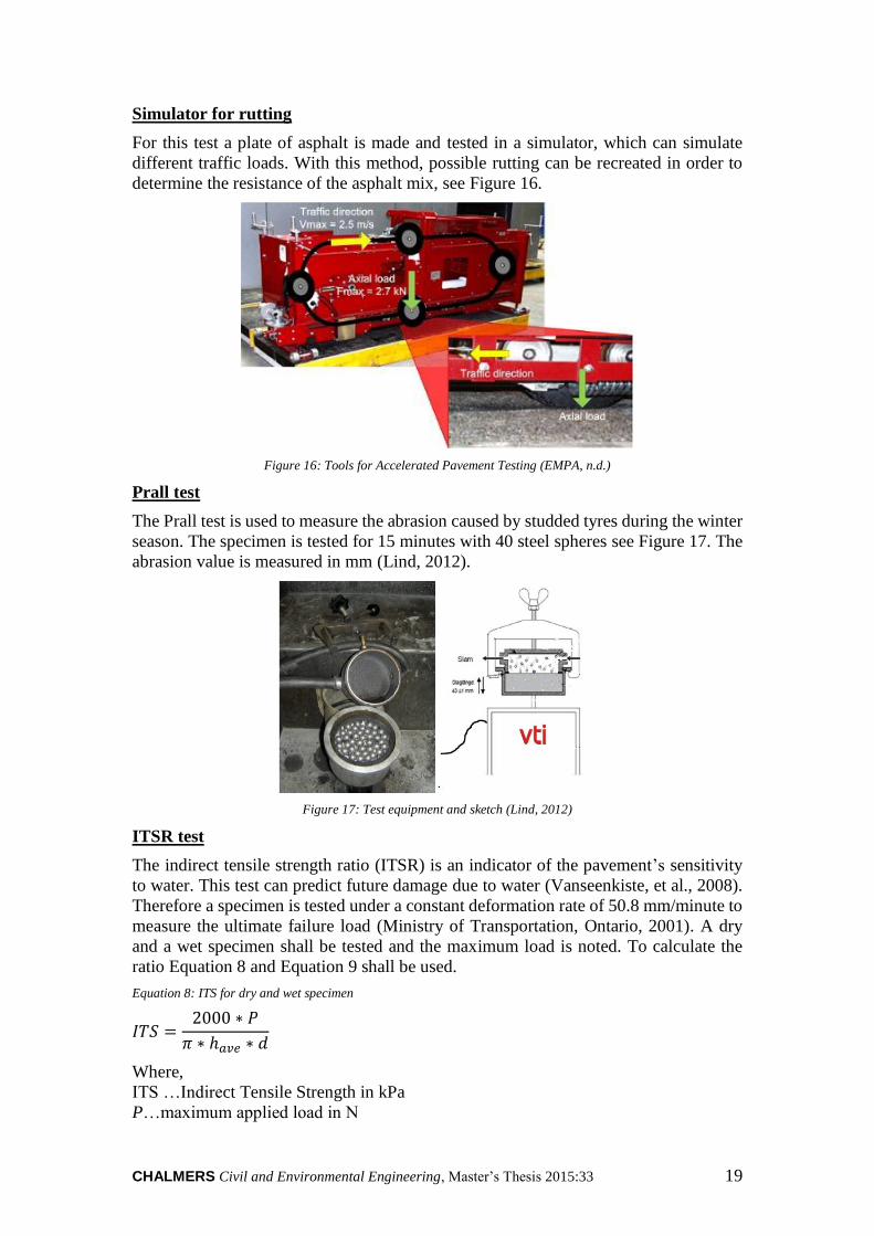
Simulator for rutting
For this test a plate of asphalt is made and tested in a simulator, which can simulate
different traffic loads. With this method, possible rutting can be recreated in order to
determine the resistance of the asphalt mix, see Figure 16.
Figure 16: Tools for Accelerated Pavement Testing (EMPA, n.d.)
Prall test
The Prall test is used to measure the abrasion caused by studded tyres during the winter
season. The specimen is tested for 15 minutes with 40 steel spheres see Figure 17. The
abrasion value is measured in mm (Lind, 2012).
Figure 17: Test equipment and sketch (Lind, 2012)
ITSR test
The indirect tensile strength ratio (ITSR) is an indicator of the pavement’s sensitivity
to water. This test can predict future damage due to water (Vanseenkiste, et al., 2008).
Therefore a specimen is tested under a constant deformation rate of 50.8 mm/minute to
measure the ultimate failure load (Ministry of Transportation, Ontario, 2001). A dry
and a wet specimen shall be tested and the maximum load is noted. To calculate the
ratio Equation 8 and Equation 9 shall be used.
Equation 8: ITS for dry and wet specimen
𝐼𝑇𝑆 =2000 ∗ 𝑃
𝜋 ∗ ℎ𝑎𝑣𝑒 ∗ 𝑑
Where,
ITS …Indirect Tensile Strength in kPa
P…maximum applied load in N

CHALMERS, Civil and Environmental Engineering, Master’s Thesis 2015:33 20
have … average height of the specimen in mm to one decimal place
d …diameter of the specimen in mm to one decimal place
Equation 9: Indirect tensile strength ratio
𝑇𝑆𝑅 = (𝐼𝑇𝑆𝑤𝑒𝑡
𝐼𝑇𝑆𝑑𝑟𝑦) ∗ 100%
Where,
ITSwet … average ITS of all wet specimens in the set
ITSdry … average ITS of all dry specimens in the set
2.4.4 Field tests
Field tests are available for different sub-layers of the road. Three are mentioned below.
Static plate bearing test
This test is for the bearing capacity of the aggregates in field. A hydraulic strength is
added to the plates and the settlements are measured depending on added load, see
Figure 18. After that a graph settlements against bearing pressure gives the bearing
capacity (Subadra Consulting Ltd, n.d.).
Figure 18: Hydraulic Jack for plate bearing capactity measurement (Iowa State University, 2015)
Falling weight deflectometer
This test can be used for the road infrastructure and each layer. It is measured to identify
the structural capacity and performance, load capacity of the road as well as it can be
used for maintenance purposes (Roadway Inventory & Testing Section (RITS), 2005)
A weight is dropped onto a load surface and the deflection of the drops is measured
with sensors in a series. A principal sketch is shown in Figure 19.
Figure 19: Sketch of FWD principal (Bast, 2010)

CHALMERS Civil and Environmental Engineering, Master’s Thesis 2015:33 21
Rutting/ Rut depth
The manual method for measuring rut depth of the road is the straightedge method,
shown in Figure 20. The maximum depth between the straightedge and the bottom of
the pavement at gauge are measured. The straightedge shall have a minimum length of
1.73 m and should be laid at the two highest points on the sides of the rut, called contact
areas, where the gauge is laid perpendicular to the straightedge and the distance can be
measures. The measurement shall be done at various places to receive the greatest
distance.
Figure 20: Rut measurement ( ASTM International, 2011)
Another option is the automatic method where laser or ultrasonic transducers, also
called profilometer, are used to measure the rut depth in mm of the transverse road
profile.
There are various technologies available including ultrasonic lasers, point lasers,
scanning lasers and optical systems. The amount of lasers can vary, for Trafikverket 15
or 17 lasers are used for the measurement. Figure 21 shows such a transducer with
lasers, however due to the amount of lasers the positions are changing. The measuring
steps vary depending on the speed of the measuring car (Mellela & Wang, 2006).
Figure 21: Multilaser/ Profilometer laser positioning (Mellela & Wang, 2006)

CHALMERS, Civil and Environmental Engineering, Master’s Thesis 2015:33 22
MPD- Mean Profile Depth
The mean profile depth can also be measured manually or with different technologies.
The manual method is the Sand patch test, in which 25 cm³ of sand are filled into the
apertures and spread (Kim, et al., 2013), shown in Figure 22. Further on the mean
texture depth (MTD) can be calculated with Equation 10. Nowadays, glass is used
instead of sand for the patch method due to it being less sensitive to moisture (Nordgren,
2015).
Figure 22: Sand Patch Test (Kim, et al., 2013)
Equation 10: Mean Texture Depth (Kim, et al., 2013)
𝑀𝑇𝐷 = 4 𝑉
𝜋 𝐷²; 𝑉 =
𝜋 𝑑² ℎ
4
where,
d … Sand diameter
h … Sand Cylinder height
Another option to measure the MPD is the portable laser profile. For this test the time
is measured, which the emitted laser needs to reflect from the pavement surface and
back to the car (Kim, et al., 2013).

CHALMERS Civil and Environmental Engineering, Master’s Thesis 2015:33 23
2.5 Trafikverket system
Trafikverket has an internal system, which is used for starting new projects, for their
follow up and for the evaluation of projects related to maintenance. This system is
composed of VU+, VUH and PMSV3 which are smaller individual, yet connected
systems, see Figure 23 (Darabian, 2015).
Figure 23: Systems in Trafikverket's working routines after (Darabian, 2015)
VU+
VU+ stands for road maintenance planning management maintenance system. It has
recently been developed and renamed to PLS paving, which means Project
Management System for paving. PLS is the tool for planning, cost estimation and
project planning as well as project follow-ups, where the stored data provides a base
for future decision making and result handling. It was developed according to
Trafikverket’s requirements in order to provide an effective tool for project leaders to
work in a uniform method (Darabian, 2015).
VUH
VUH (vägunderhållsdata) is an abbreviation for road maintenance data and forms the
database where all paving data is stored and used as input for other systems (Darabian,
2015).
PMSV3
PMSV3 (Pavement Management System) is the third part of the system and provides
information about the state road-network surface conditions. The data stored in VUH
and other databases forms the input for several querying functions, such as IRI, rut
depth, texture and other forms of deformation. Data can be retrieved for many stretches
and illustrated in form of tables, graphs, maps and pictures. This enables the assessment
of necessary maintenance measures at the right place and right time. Moreover it is
Trafikverket’s tool for following up previous projects and evaluating maintenance
methods as well as it is open to the public (Trafikverket, 2014).

CHALMERS, Civil and Environmental Engineering, Master’s Thesis 2015:33 24
2.6 Road surveys
The road surveys are necessary to determine the current state of the road. The roads are
investigated for different deformations and damages such as cracks, texture, rut depths,
IRI and many other parameters. In the chapter below the most relevant survey methods
for this project are presented, as well as their differences.
2.6.1 PMSV3 Road network measurement
The data in the PMSV3 are recorded from a single measurement, using a specially
equipped car with 17 lasers. However, measurements from 15 lasers exclude possible
measurements from the verges and other irregularities. Moreover, the lane widths are
shrinking which makes measurements with 15 lasers more suitable (Nordgren, 2015).
The measurements are done during normal traffic conditions. The lasers record one
value for rutting (rut max15) and MPD right, middle and left (mean profile depth) each
20 meters (Nordgren, 2015).
2.6.2 Object measurement (Objektsmätning)
For the Objektsmätning a car with similar equipment is used as for the survey for
PMSV3. The difference is that each section is measured 3 times, which provides a
higher degree of certainty for the measurements. From these three measurements an
average value is determined. The measuring car is driven at traffic speed, without
closing down the road in usual traffic condition. The cost for this survey type lies
between 20,000 to 30,000 SEK for 5 to 10 km of measured track (Nordgren, 2015).
2.6.3 VTI
VTI uses more advanced measurements. The roads are closed in order to avoid any
disturbances from traffic. For measuring the surface wearing (especially from studded
tires) a laser profile meter is used that measures the profiles in estimated 1240 points
per cross section (415 points per meter) see Figure 24. Moreover an area of 1m2 is
marked and divided into 11 lines, which is measured each year. The goal with these
procedures is to help identifying how much aggregates are torn out each year and how
resilient the wearing course is.
Figure 24: Laser profile meters (Karlsson, 2015)
Profiles are measured with Primal (Figure 25), a method where sampling points are
marked with colour and a steel nail to be sure the same spot is measured each time. A

CHALMERS Civil and Environmental Engineering, Master’s Thesis 2015:33 25
robot rolls from the middle line between the lanes and moves towards the verge, taking
measurements each 4th millimetre. The cost for this survey is much higher than for the
Objektsmätning and can be for 5 to 10 km up to 100’000 SEK on a high traffic road
(Nordgren, 2015).
Figure 25: Profile cross section measurement with Primal (Karlsson, 2015)
2.7 Requirements from Trafikverket and VTI
Trafikverket’s standards and regulations for the entire production process of asphalt
products are based on the European standards. These regulations define material
properties and proportions in asphalt mixtures. Testing methods and the paving
procedures have to be performed in a regulated and secure way. Moreover, once the
road is constructed it should fulfil required qualities and last for the planned time frame.
The work is controlled frequently with sampling, laboratory tests and onsite tests to
assure the correct quality of the material, material composition and implementation of
working routines.
2.7.1 Aggregates
The mixing process is very crucial in the asphalt production regarding the product. In
the mixing process time and temperature are very important regarding the binding
properties and have to be monitored with great care. Binding ability for asphalt,
independent of type, deteriorates the longer it is stored and it should therefore be
transported to the working site as soon as possible (Nordgren, 2014).
Conventional hot mix- asphalt has the requirement to be produced in a batch- or drum
mix plant with a temperature exceeding 120˚C (Trafikverket, 2005).
Table 1 below shows the required standards for stone aggregates in the asphalt mix.
Table 1: Testing standards for stone aggregates (Trafikverket, 2005)
Testing method Standard
SS-EN
Tested stone material
Test fraction
Nordic abrasion test 1097-9 11,2 - 16 mm
Micro Deval value 1097-1 10 – 14 mm
Los Angeles value 1097-2 10 – 14 mm
Flakiness index 933-3 ≥ 4 mm
Proportion of grains with broken and
crushed surface 933-5 ≥ 4 mm

CHALMERS, Civil and Environmental Engineering, Master’s Thesis 2015:33 26
2.7.2 Deformations
Mean profile depth (MPD) and rutting
Trafikverket and VTI have assembled requirements for the mean profile depth and rut
depth to make a classification of MPD and rutting values possible.
In the tables below the quality of the road and the effects are presented related to MPD
intervals.
Table 2: VTI classification of MPD with speed limits, considering texture (Lundberg, et al., 2011)
MPD- area in mm Velocity 90-100
km/h Velocity 70 km/h Velocity 30-50 km/h
0-0.30 mm Bad
0,31–0,50 mm Bad Good
0,51–0,70 mm Bad Excellent Excellent
0,71–1,00 mm Excellent Acceptable Acceptable
1,01–1,50 mm Excellent Bad Bad
1,51–2,00 mm Acceptable Bad
2,01–mm Bad
There are many more measurements that can be used for classification; however we
chose to limit our choice to these in order to stay within the scope of the study.
Table 2 above is retrieved from VTI and modified so they fit this study. Modified means
data that is not relevant for MPD or rutting was removed (Lundberg, et al., 2011).
Trafikverket has requirements and standards for MPD and rutting as well, which are
presented in the Table 3 and Table 4 below (Trafikverket Underhållsstandard, 2012).
Table 3: Trafikverket requirements for MPD based on traffic volumes and speed limits (Trafikverket
Underhållsstandard, 2012)
Traffic (vehicles/day)
Lowest MPD [mm] according to speed limit (km/h)
120 110 100 90 80 70 60 50
0-250
250- 500
500- 1000
1000- 2000
2000- 4000
4000- 8000
>8000
≥ 0.20 ≥ 0.20 ≥ 0.20 ≥ 0.20 ≥ 0.20 ≥ 0.20 ≥ 0.20
≥ 0.25 ≥ 0.25 ≥ 0.25 ≥ 0.25 ≥ 0.20 ≥ 0.20 ≥ 0.20
≥ 0.30 ≥ 0.30 ≥ 0.30 ≥ 0.25 ≥ 0.25 ≥ 0.25 ≥ 0.25
≥ 0.33 ≥ 0.33 ≥ 0.33 ≥ 0.28 ≥ 0.28 ≥ 0.28 ≥ 0.28
≥ 0.35 ≥ 0.35 ≥ 0.35 ≥ 0.35 ≥ 0.30 ≥ 0.30 ≥ 0.30 ≥ 0.30
≥ 0.35 ≥ 0.35 ≥ 0.35 ≥ 0.35 ≥ 0.30 ≥ 0.30 ≥ 0.30 ≥ 0.30
≥ 0.40 ≥ 0.40 ≥ 0.40 ≥ 0.40 ≥ 0.35 ≥ 0.35 ≥ 0.35 ≥ 0.35
Table 4: Trafikverket requirements for rutting based on traffic volumes and speed limits (Trafikverket
Underhållsstandard, 2012)
Traffic (vehicles/day) Maximum rutting [mm] according to speed limit (km/h)
120 110 100 90 80 70 60 50
0-250
250- 500
500- 1000
1000- 2000
2000- 4000
4000- 8000
>8000
≤ 18.0 ≤ 18.0 ≤ 24.0 ≤ 24.0 ≤ 30.0 ≤ 30.0 ≤ 30.0
≤ 18.0 ≤ 18.0 ≤ 22.0 ≤ 22.0 ≤ 22.0 ≤ 22.0 ≤ 22.0
≤ 18.0 ≤ 18.0 ≤ 20.0 ≤ 20.0 ≤ 24.0 ≤ 24.0 ≤ 24.0
≤ 15.0 ≤ 16.0 ≤ 17.0 ≤ 18.0 ≤ 20.0 ≤ 21.0 ≤ 21.0
≤ 13.0 ≤ 13.0 ≤ 14.0 ≤ 14.0 ≤ 16.0 ≤ 16.0 ≤ 18.0 ≤ 18.0
≤ 13.0 ≤ 13.0 ≤ 14.0 ≤ 14.0 ≤ 16.0 ≤ 16.0 ≤ 18.0 ≤ 18.0
≤ 13.0 ≤ 13.0 ≤ 14.0 ≤ 14.0 ≤ 16.0 ≤ 16.0 ≤ 18.0 ≤ 18.0

CHALMERS Civil and Environmental Engineering, Master’s Thesis 2015:33 27
3 Method
The project was mainly built up on collecting literature from Trafikverket, VTI and
international road administrations. With this data a literature review was formed with
necessary information to understand the results.
Afterwards tracks with RMA were searched with help of the analysis tool in PMSV3,
which can filter out tracks according to properties such as wearing course type. For the
analysis on the parameters texture (MPD) and rut depth were used, since these two
parameters are the most important ones for Trafikverket to determine the quality and
condition of the wearing course. These properties are also used for the comparison of
different asphalt types.
An analysis template in excel was programed to analyse and sort the data according to
asphalt type, years and traffic volumes. Sorting the data by these variables enabled
filtering out the sections, which were placed on the same date and had similar, if not
equal traffic volumes. When this was achieved the two asphalt types could be compared
for rut depth and texture with equal conditions. Since most of the sections included
thousands of values, the average values for each section were calculated in addition to
the average annual increase/ decrease, standard deviation, maximum and minimum
value as well as the variance.
Afterwards the results were controlled if they fulfilled Trafikverket’s and VTI’s
requirements for maximum allowed rut depth and minimum allowed MPD and when
the next maintenance would be necessary. The years until next maintenance were
calculated according to Equation 11 below and helped determine, which asphalt type
lasts longer.
Equation 11: Years until next maintenance based on rut depth
𝑙𝑎𝑠𝑡 𝑚𝑒𝑎𝑠𝑢𝑟𝑒𝑑 𝑟𝑢𝑡 𝑑𝑒𝑝𝑡ℎ [𝑚𝑚] − 𝑚𝑎𝑥𝑖𝑚𝑢𝑚 𝑎𝑙𝑙𝑜𝑤𝑒𝑑 𝑟𝑢𝑡 𝑑𝑒𝑝𝑡ℎ[𝑚𝑚]
𝑎𝑣𝑒𝑟𝑎𝑔𝑒 𝑣𝑎𝑙𝑢𝑒 𝑓𝑜𝑟 𝑎𝑛𝑛𝑢𝑎𝑙 𝑐ℎ𝑎𝑛𝑔𝑒 𝑠𝑖𝑛𝑐𝑒 𝑙𝑎𝑡𝑒𝑠𝑡 𝑚𝑎𝑖𝑛𝑡𝑒𝑛𝑎𝑛𝑐𝑒 [𝑚𝑚/𝑦𝑒𝑎𝑟]
The classification of the texture was based on the last measured left and right MPD,
which were in the contact areas of the tires on the asphalt. MPD middle could be used
as an indicator for the climate impact on the surface, since this area is not exposed to
the same contact frequency with tyres as the left and right side.
The next step was the assessment of PMSV3 as an analysis tool, where the measured
results were compared to those from Objektsmätning on the E4 in Uppsala and from
the analysis on the RV47 in Falköping from VTI. The results were expressed as a
deviation in form of percent. Depending on the outcome PMSV3 was judged for its
suitability for further analysis.
CHALMERS, Civil and Environmental Engineering, Master’s Thesis 2015:33 28
4 Analysis and verification of results for asphalt
All data that has been analysed will be gathered in this chapter and explained. The
results will mainly be presented in form of diagrams and tables, with focus on rut depth
and MPD. The rubber modified asphalt and the standard asphalt will be compared
according to their resistance against wearing caused by traffic. Moreover the sections
will be checked for Trafikverket’s (Table 3 & Table 4) and VTI’s (Table 2)
classification and requirements in addition to the remaining time before the next
maintenance. The majority of the investigated tracks were covered with standard
asphalt and rubber modified asphalt, since they were the focus of study for this thesis.
Other types were nevertheless also included, such as polymer modified asphalt, partly
due to their presence in the analysed sections and partly due to curiosity.
The data for most of the tracks was retrieved from PMSV3 in this project. Additionally
for the quality verification of PMSV3, measurements from Objektsmätning were used.
The comparison to Objektsmätning will be mentioned; otherwise the results are based
on PMSV3. More details about the measurement procedure and equipment are
explained in Chapter 2.6
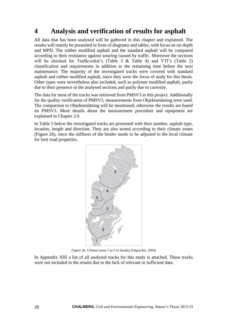
In Table 5 below the investigated tracks are presented with their number, asphalt type,
location, length and direction. They are also sorted according to their climate zones
(Figure 26), since the stiffness of the binder needs to be adjusted to the local climate
for best road properties.
Figure 26: Climate zones 1 to 5 in Sweden (Vägverket, 2004)
In Appendix XIII a list of all analysed tracks for this study is attached. These tracks
were not included in the results due to the lack of relevant or sufficient data.

CHALMERS Civil and Environmental Engineering, Master’s Thesis 2015:33 29
Table 5: List of tracks used for the investigation according to climate zone
Road
no.
Climate
zone
Location Direction Start-and
Stoppoint
Asphalt type Lanes Speed
limit
[km/h]
E4 1 Kropp-Hyllinge Med 15870-
20415
ABS 70/100 B
GAP 70/100 B 10, 20 110
E6 1 Fredriksberg-
Lockarp Mot
108091-
112673
ABS 70/100 B
GAP 70/100 B 10, 20 110
E6 1 Kronetorp-Salerup Mot 98965-
105524
ABS 70/100 B
GAP 70/100 B 10, 20 110
E6 1 Petersborg-
Vellinge South Mot
115947-
125955
ABS 70/100 B
GAP 70/100 B 10, 20 110
E6 1 Sunnanå-
Kronetorp Med
36016-
41005
ABS 70/100 B
GAP 70/100 B 10, 20 110
E6 2 Ullevi-Kallebäck Med 176896-
179689
ABS 70/100 PMB
GAP 70/100 B 10, 20 70
RV47 2 Falköping Med 21220-
23720
ABT 70/100 B
PMB, 6 types 10 80
E4 2 Uppsala-Knivsta Med 84720-
101445
GAP16 0.6% Wetfix
10, 20 110
GAP16 0.6% Wetfix
Pt2
GAP 16% 0.3%
Wetfix 1% Cement
GAP 16% Increased
Temp
ABS 70/100
ABS 50/70
GAP 16 Increased
Temp Pt2
E4 2 Viby-Sollentuna,
Stockholm Mot
27317-
30873
ABS 70/100 B
GAP 70/100 B 30 110
E4 4 Broänge-Hökmark Med 156720-
164260
GAP16 100/150
ABS 16 100/150 10 90
E12 4 Lycksele Med 151932-
158798
ABTS 11
ABTS 11 GMB 10 50-90
E12 4 Lycksele Mot 307155-
309235
ABTS 11
ABTS 11 GMB 10 50-90
E12 4 Storuman-Stensele Med 245181-
252932
GAP 16
ABT 16 GMB
ABT 16 B 160/220
10 50-90
E4 5 Gäddvik-Nickbyn Med 72795-
89450
GAP 16
ABS 16 100/150 10 110
E4 5 Gäddvik-Nickbyn Mot 112038-
130608
ABS 16 GMB
ABS 16 100/150 10 110

CHALMERS, Civil and Environmental Engineering, Master’s Thesis 2015:33 30
4.1 Climate Zone 1
Climate zone 1 is the southernmost zone in Sweden with the warmest temperatures
during the year. In this zone cities such as Malmö, Helsingborg and Kristianstad are
located.
4.1.1 E4 Kropp- Hyllinge med
This road section is located north east of Helsingborg with a length of 13.4 kilometres
(Figure 27). The speed limit is 110 km/h and the traffic volume varies between 4500,
13383 and 11734 vehicles per day, (Trafikverket, 2015). A standard asphalt ABS
70/100 B and a rubber- modified asphalt GAP 70/100 B were placed in June 2010. In
the figures below the results are sorted according to traffic to enable a direct
comparison.
Figure 27: E4 Kropp- Hyllinge, 15870- 20415 (Trafikverket PMSV3, 2015)

CHALMERS Civil and Environmental Engineering, Master’s Thesis 2015:33 31
KF 10
Figure 82 and Figure 83 in Appendix I: E4 Kropp-Hyllinge provide an overall picture
of the average rutting and MPD values along the road. In general the road is covered
with GAP and the part with ABS is relatively small, which can influence the average
values. The rut depths are greater for GAP, while the MPD is higher for ABS. The
peaks in the graph could not be related to potholes or major deformations on the road
surface since PMSV3 did not show such.
The values in Figure 28 and Figure 29 deviate between 18- 40% from the average
values, which indicates an uneven rut pattern.
Figure 28: Average values and Standard deviation of rutting on GAP and ABS, high traffic volumes
Figure 29: Average values and standard deviation of rutting on GAP and ABS, low traffic volume
In Figure 30 below the sections for standard ABS and the rubber- modified asphalt were
sorted by the traffic volume and compared. The ABS was placed in 2010 after the road
measurement, which explains the high values in 2010. Thereafter the increase in rut
depth can be followed for each year.

CHALMERS, Civil and Environmental Engineering, Master’s Thesis 2015:33 32
Figure 30: Average values and annual change for rutting on standard ABS and GAP
According to the figure above the rut depth on the GAP increased more slowly than the
ABS in 2011 and 2012. It increased on an average of 1 mm per year. In 2014 the rut
depths on the GAP became higher than on the ABS on the section with 4500 vehicles
per day, however on the other sections the rutting on the ABS remained higher although
the traffic there is lower.
In Appendix I: E4 Kropp-Hyllinge Figure 84, Figure 85 and Figure 86 the mean profile
depth was measured for the left, middle and right part of the lane. In all three figures
the MPD values are higher for the ABS than for the GAP, independent of traffic.
Table 6 below shows the current state for the investigated road and if VTI’s and
Trafikverket’s recommendations are fulfilled. The average value from all years for the
rate of change on rutting will be used to estimate when the next maintenance is
necessary, starting from the last measured year.
Table 6: Current state and classification for E4 Kropp- Hyllinge KF10 according to VTI and Trafikverket
Section
Trafikverket VTI
(0.71-2.00
mm)
Years to next
maintenance Rutting
(13mm)
MPD
(0.40mm/
0.35mm)
GAP 13383 Yes Yes Bad 7
ABS 11734 Yes Yes Excellent 7
GAP 4500 Yes Yes Bad/Excellent 14.5
ABS 4500 Yes Yes Excellent 23
Comparing the remaining years to maintenance, the GAP and ABS have equal lifetime
although the traffic is higher on the section with GAP. On the section with 4500
vehicles per day the lifetime for the ABS is longer by 8.5 years.

CHALMERS Civil and Environmental Engineering, Master’s Thesis 2015:33 33
KF 20
The same description applies to this lane as for the first lane regarding location, traffic
and materials.
According to Figure 87 and Figure 88 in Appendix I: E4 Kropp-Hyllinge the rutting is
more extreme for the ABS than for the GAP. However, the difference is related to the
age of the ABS, which was placed in 1994 compared to the GAP in 2010 according to
PMSV3. To approve this statement these dates have to be verified since the measured
values resemble those of newer asphalt compared to the other sections.
The measurements on this lane differ from those on the first lane. The ABS has much
higher rutting and a much higher standard deviation than the GAP (Figure 31).
Figure 31: Average values and standard deviations for rutting, MPD left, middle and right on ABS and GAP
Knowing that there was a difference in time when the asphalts were laid, the average
values are not comparable. On the other hand the rate of change in Figure 32 provides
information on how fast the two surface layers deteriorate. According to the rate of
change in 2012 the rut depth increases by 0.73 mm for the GAP and 0.56 mm for the
ABS in two years. In 2014 the rut depth increased by 0.74 mm for the GAP and 0.87
mm for the ABS in two years.
Figure 32: Average values and rate of change for rutting on GAP and ABS

CHALMERS, Civil and Environmental Engineering, Master’s Thesis 2015:33 34
In Appendix I: E4 Kropp-Hyllinge Figure 89, Figure 90 and Figure 91 the MPD’s were
measured. In general ABS has higher values than the GAP except for the right MPD;
however for both there was no significant change visible through the years.
Table 7: Current state and classification for E4 Kropp- Hyllinge KF20 med, according to VTI and Trafikverket
Section
Trafikverket VTI
(0.71-2.00
mm)
Years to next
maintenance Rutting
(13mm)
MPD
(0.40mm)
GAP 13383 Yes Yes Excellent 27.8
ABS 11734 Yes Yes Excellent 28.1
GAP 4500 Yes Yes Excellent 33.4
ABS 4500 Yes Yes Excellent 22.9
According to Table 7 the GAP 13383 lasts two years less than the ABS 11734. At 4500
vehicles per day the GAP has 10.5 years longer lifetime than ABS. According to last
years’ measurements the texture is very similar for both types and in excellent
condition.
4.1.2 E6 Fredriksberg- Lockarp KF10 & 20 mot
This section of the E6 is located in the south of Malmö and has a speed limit of 110
km/h (Figure 33). The road is covered with a standard ABS 70/100 B and rubber-
modified asphalt GAP 70/100 B. The road was separated in sections with traffic
volumes of 7157, 17064 and 19089 vehicles per day (Trafikverket, 2015). The ABS
was placed in 2010 and the GAP in 2009.
Figure 33: E6 Fredriksberg- Lockarp, 108091- 112673 (Trafikverket PMSV3, 2015)

CHALMERS Civil and Environmental Engineering, Master’s Thesis 2015:33 35
KF 10
Figure 92 and Figure 93 in Appendix II: E6 Fredriksberg-Lockarp Appendix II: E6
Fredriksberg-Lockarp demonstrate the road condition regarding rutting and MPD and
were separated according to similar traffic in order to evaluate each asphalt type’s
resistance to wearing. The reason for the high peak in the end of each measurement for
the GAP is unknown.
Figure 34: Average values and rate of change for rutting on GAP and ABS with traffic volume of 7157 vehicles per
day
The difference between GAP and ABS becomes clear in Figure 34. The initial rutting
for the GAP is higher than the initial rutting for the ABS (2010). Apart from that the
GAP deteriorates faster than the ABS as the average rate of change proves.
In the sections with higher traffic the picture changes. As illustrated in Figure 35 the
rutting is larger for ABS than for GAP, however this can be related to the higher traffic
on the ABS section.
Figure 35: Average values and rate of change for rutting on GAP and ABS with traffic volume of 17064 and 19089
vehicles per day
Figure 94, Figure 95 and Figure 96 in Appendix II: E6 Fredriksberg-Lockarp represent
the average MPD values on the left, middle and right part of the lane. The values on the
section with 19089 vehicles per day are lower for the ABS, which can be related to the
high traffic intensity compared to the other sections. The remaining sections have a

CHALMERS, Civil and Environmental Engineering, Master’s Thesis 2015:33 36
more or less constant average value and a low changing rate. Another observation is
higher rutting on the GAP at lower traffic volumes.
Table 8: Current state and classification for E6 Fredriksberg- Lockarp KF10 mot, according to VTI and
Trafikverket
Section
Trafikverket VTI
(0.71-2.00
mm)
Years to next
maintenance Rutting
(13mm)
MPD
(0.40mm)
GAP 17064 Yes Yes Excellent 29,6
ABS 19089 Yes Yes Bad 13
GAP 7157 Yes Yes Excellent 24.2
ABS 7157 Yes Yes Excellent 21.6
In Table 8 the sections are put into classes according to the VTI classification system.
All sections are rated with excellent except for the ABS on with 19089 vehicles per day
on the left and right MPD. On that section the road quality was severely degraded after
2010.
At the sections with higher traffic the GAP lasts over 16 years longer than the ABS. On
the section with lower traffic the GAP provides a longer lifetime as well, by 2.6 years.
KF 20
The measurements for the second lane are made each second year. In Figure 36 below
the rut depths from 2010 to 2014 can be compared for the different sections. On the
sections with higher traffic, the rut depths on the rubber modified asphalt are smaller
than on the standard asphalt. The rate of change is larger for the ABS, which is an
indicator for faster deterioration. On the other sections the rut depth are very similar.
Figure 36: Average values and rate of change for rutting on GAP and ABS
Figure 97 and Figure 98 in Appendix II: E6 Fredriksberg-Lockarp show the MPD
values for the left and middle track. On the right MPD the ABS at 19089 vehicles per
day is significantly low compared to the others in Figure 99 (Appendix II: E6
Fredriksberg-Lockarp), but still within the interval for excellent quality. The ABS at
19089 vehicles per day has the lowest values for texture.
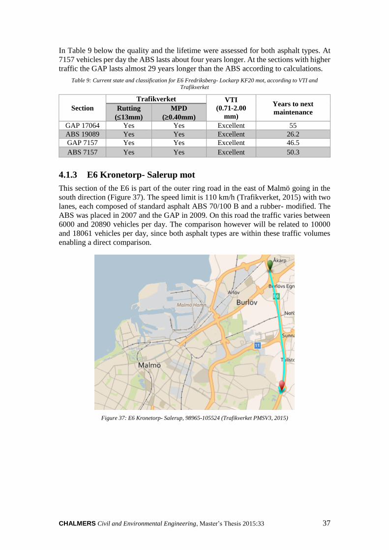
CHALMERS Civil and Environmental Engineering, Master’s Thesis 2015:33 37
In Table 9 below the quality and the lifetime were assessed for both asphalt types. At
7157 vehicles per day the ABS lasts about four years longer. At the sections with higher
traffic the GAP lasts almost 29 years longer than the ABS according to calculations.
Table 9: Current state and classification for E6 Fredriksberg- Lockarp KF20 mot, according to VTI and
Trafikverket
Section
Trafikverket VTI
(0.71-2.00
mm)
Years to next
maintenance Rutting
(13mm)
MPD
(0.40mm)
GAP 17064 Yes Yes Excellent 55
ABS 19089 Yes Yes Excellent 26.2
GAP 7157 Yes Yes Excellent 46.5
ABS 7157 Yes Yes Excellent 50.3
4.1.3 E6 Kronetorp- Salerup mot
This section of the E6 is part of the outer ring road in the east of Malmö going in the
south direction (Figure 37). The speed limit is 110 km/h (Trafikverket, 2015) with two
lanes, each composed of standard asphalt ABS 70/100 B and a rubber- modified. The
ABS was placed in 2007 and the GAP in 2009. On this road the traffic varies between
6000 and 20890 vehicles per day. The comparison however will be related to 10000
and 18061 vehicles per day, since both asphalt types are within these traffic volumes
enabling a direct comparison.
Figure 37: E6 Kronetorp- Salerup, 98965-105524 (Trafikverket PMSV3, 2015)

CHALMERS, Civil and Environmental Engineering, Master’s Thesis 2015:33 38
KF10
Figure 38: Average values and rate of change for rutting on GAP and ABS
From Figure 38 above it is possible to see that the ABS has higher rut depths than the
GAP at both traffic volumes and all years, except for 2010 where the rubber modified
asphalt has higher initial rutting. Another observation is that the rut depth is higher for
the GAP at lower traffic volumes.
According to Figure 100, Figure 101 and Figure 102 in Appendix III: E6 Kronetorp-
Salerup the MPD values for the left, middle and the right part of the lane are excellent
for GAP according to VTI (>0.71 mm), approximately 1.1 mm. The ABS (0.55 mm) is
under the lower limit required by VTI and classified as bad. Both however fulfil
Trafikverket’s requirements to be larger than 0.4 mm.
In Table 10 the tracks are evaluated according to Trafikverket’s and VTI’s classification
system. The rubber modified asphalt offers better texture and rut resistance according
to the calculated values. Comparing it to the standard asphalt it has 16 years longer
lifetime at 18618 vehicles per day and 14.1 years longer lifetime at 10000 vehicles per
day.
Table 10: Current state and classification for E6 Kronetorp- Salerup KF10 mot, according to VTI and Trafikverket
Section
Trafikverket VTI
(0.71-2.00
mm)
Years to next
maintenance Rutting
(13mm)
MPD
(0.40mm)
GAP 18618 Yes Yes Excellent 26.3
ABS 18618 Yes Yes Bad 10.3
GAP 10000 Yes Yes Excellent 23.8
ABS 10610 Yes Yes Bad 9.7

CHALMERS Civil and Environmental Engineering, Master’s Thesis 2015:33 39
KF20
For the second lane measurements are made each second year. The results are presented
in the figures and tables below. From the data it can be seen that for the second lane,
the results are the other way round (Figure 39). The ABS indicates lower rut depths for
both traffic volumes throughout the years.
Figure 39: Average values and rate of change for rutting on ABS and GAP
Both asphalt types fulfil Trafikverket’s and VTI’s requirements for excellent texture.
The rubber modified asphalt has yet greater MPD’s. As Figure 103, Figure 104 and
Figure 105 in Appendix III: E6 Kronetorp-Salerup indicate, the ABS and GAP have
similar quality in the section with 10000 vehicles per day. Table 11 below summarizes
the results. At the section with 18618 vehicles per day the standard asphalt lasts almost
14 years longer, while the lifetime is the same (26.4 years) at 10000 vehicles per day.
Table 11: Current state and classification for E6 Kronetorp- Salerup KF20 mot, according to VTI and Trafikverket
Section
Trafikverket VTI
(0.71-2.00
mm)
Years to next
maintenance Rutting
(13mm)
MPD
(0.40mm)
GAP 18618 Yes Yes Excellent 26.1
ABS 18618 Yes Yes Excellent 40.4
GAP 10000 Yes Yes Excellent 26.4
ABS 10610 Yes Yes Excellent 26.4

CHALMERS, Civil and Environmental Engineering, Master’s Thesis 2015:33 40
4.1.4 E6 Petersborg- Vellinge KF10 & 20 mot
This track is located in Skåne, in the South of Malmö with coordinates between 115947
and 125955 (Figure 40). The road has two lanes with a speed limit of 110 km/h
(Trafikverket, 2015). A standard ABS 70/100 B and a rubber modified asphalt GAP
70/100 B were used and placed in 2009. The traffic varies between 3250 vehicles per
day and 19364 vehicles per day. The sections with equal traffic are at 17132 vehicles
per day, which is the reason why only this section will be analysed and compared. On
this section the length of the GAP part is 600 meters and 600 meters for the ABS.
Figure 40: E6 Petersborg- Vellinge, 115947-125955 (Trafikverket PMSV3, 2015)
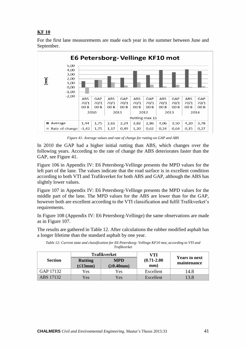
CHALMERS Civil and Environmental Engineering, Master’s Thesis 2015:33 41
KF 10
For the first lane measurements are made each year in the summer between June and
September.
Figure 41: Average values and rate of change for rutting on GAP and ABS
In 2010 the GAP had a higher initial rutting than ABS, which changes over the
following years. According to the rate of change the ABS deteriorates faster than the
GAP, see Figure 41.
Figure 106 in Appendix IV: E6 Petersborg-Vellinge presents the MPD values for the
left part of the lane. The values indicate that the road surface is in excellent condition
according to both VTI and Trafikverket for both ABS and GAP, although the ABS has
slightly lower values.
Figure 107 in Appendix IV: E6 Petersborg-Vellinge presents the MPD values for the
middle part of the lane. The MPD values for the ABS are lower than for the GAP,
however both are excellent according to the VTI classification and fulfil Trafikverket’s
requirements.
In Figure 108 (Appendix IV: E6 Petersborg-Vellinge) the same observations are made
as in Figure 107.
The results are gathered in Table 12. After calculations the rubber modified asphalt has
a longer lifetime than the standard asphalt by one year.
Table 12: Current state and classification for E6 Petersborg- Vellinge KF10 mot, according to VTI and
Trafikverket
Section
Trafikverket VTI
(0.71-2.00
mm)
Years to next
maintenance Rutting
(13mm)
MPD
(0.40mm)
GAP 17132 Yes Yes Excellent 14.8
ABS 17132 Yes Yes Excellent 13.8

CHALMERS, Civil and Environmental Engineering, Master’s Thesis 2015:33 42
KF20
On the second lane the road is measured each second year.
Figure 42: Average values and rate of change for rutting on GAP and ABS
Figure 42 above provides the same results as in Figure 41. Here as well, the rubber-
modified asphalt has lower rutting than the ABS, in addition to a lower rate of change
Figure 109, Figure 110 and Figure 111 in Appendix IV: E6 Petersborg-Vellinge prove
the same results as the MPD values in the first lane. Both asphalt types fulfil
Trafikverket’s and VTI’s requirements except the ABS in the middle part, which is
lower than the VTI requirements.
Table 13: Current state and classification for E6 Petersborg- Vellinge KF20 mot, according to VTI and
Trafikverket
Section
Trafikverket VTI
(0.71-2.00
mm)
Years to next
maintenance Rutting
(13mm)
MPD
(0.40mm)
GAP 17132 Yes Yes Excellent 36.8
ABS 17132 Yes Yes Excellent 29.2
Both asphalt types offer a good performance according to Trafikverket’s requirements
and fulfil the VTI requirements for excellent classification, regarding MPD as well
(Table 13). The rubber modified asphalt proved to be more resilient than the ABS both
in rutting and texture on both lanes and lasts 7.6 years longer.

CHALMERS Civil and Environmental Engineering, Master’s Thesis 2015:33 43
4.1.5 E6 Sunnanå- Kronetorp KF10 & 20 med
This track is located in the north of Malmö going in the north direction (Figure 43). The
coordinates stretch from 36016 to 41005 with a standard asphalt ABS 70/100 B and a
rubber modified asphalt GAP 70/100 B. The speed limit is 110 km/h along the whole
track and has a traffic volume varying between 6000 and 20683 vehicles per day
(Trafikverket, 2015). It is only relevant to compare sections with the same or similar
traffic, therefore a section with 17012 vehicles per day was chosen for the ABS and a
section with 18294 for the GAP. At these traffic volumes the ABS section is 1020
meters long and the GAP section is 886 meters long. The ABS was placed in 2006 and
the GAP was placed in 2009.
Figure 43: E6 Sunnanå- Kronetorp, 36016-41005 (Trafikverket PMSV3, 2015)
KF 10
Figure 44: Average values and rate of change for rutting on GAP and ABS

CHALMERS, Civil and Environmental Engineering, Master’s Thesis 2015:33 44
In Figure 44 the rate of change is presented for GAP and ABS in addition to the rut
depths. A comparison for the rut depths on these sections is difficult due to the different
paving dates. Another way to compare them is analysing the rates of change. In 2011
and 2013 the rate of change on ABS is higher than on GAP. In 2012 and 2014 however
it is the other way around.
Figure 112, Figure 113 and Figure 114 in Appendix V: E6 Sunnanå-Kronetorp show
that the changes in MPD are very small during years.
Table 14: Current state and classification for E6 Sunnanå- Kronetorp KF10 med, according to VTI and
Trafikverket
Section
Trafikverket VTI
(0.71-2.00
mm)
Years to next
maintenance Rutting
(13mm)
MPD
(0.40mm)
GAP 18294 Yes Yes Excellent 26.3
ABS 17012 Yes Yes Excellent 6.6
In Table 14 the results are gathered. Both types have an excellent texture according to
classification by VTI, except for the left MPD on the ABS, which is lower than the
limit. Both fulfil Trafikverket’s requirements as well. Considering rutting, the rubber
modified asphalt would last 20 years longer than the standard asphalt.
KF 20
The traffic on the second lane is the same and even the same materials were used in the
same order. Measurements were done each second year. Figure 45 describes the
average values and rate of change for rutting from 2010 to 2014. On this lane the results
are clearer than on the first one. The rate of change for the GAP is higher than for the
ABS indicating that it is deteriorating almost twice as fast. This could once again be
related to the higher traffic, which is higher by more than 1200 vehicles per day.
Figure 45: Average values and rate of change for rutting on GAP and ABS
For the MPD values Figure 115, Figure 116 and Figure 117 in Appendix V: E6
Sunnanå-Kronetorp show the same patter as the first lane. The GAP has higher MPD’s
than the ABS, which means the texture is better and offers better riding quality.
According to Table 15, the ABS lasts over eight years longer than the rubber modified
asphalt. The texture on the other hand is better for the GAP although the traffic is higher.

CHALMERS Civil and Environmental Engineering, Master’s Thesis 2015:33 45
Table 15: Current state and classification for E6 Sunnanå- Kronetorp KF10 med, according to VTI and
Trafikverket
Section
Trafikverket VTI
(0.71-2.00
mm)
Years to next
maintenance Rutting
(13mm)
MPD
(0.40mm)
GAP 18294 Yes Yes Excellent 21.6
ABS 17012 Yes Yes Excellent 30
4.2 Climate Zone 2
Climate zone 2 is located north of the first zone with a milder temperature. Some of
Sweden’s largest cities are located in this area such as Stockholm, Gothenburg, Uppsala
and Jönköping. These cities have the largest traffic flows which puts the highest
demands on the asphalt. In this climate zone both rubber modified and polymer
modified asphalts are tested and evaluated.
4.2.1 E6 Ullevi- Kallebäck
The E6 road is located in Gothenburg stretching from Ullevi to Kallebäck junction
(Figure 46). The first and second lanes are composed of two asphalt types. The first one
is a 70/100- 48 PMB2 asphalt (placed 2011), followed by a rubber modified asphalt
with a 70/100 bitumen binder (placed 2011). The third lane is covered with GAP only
and for this reason will not be included in the analysis since it could not be compared
to another asphalt type.
Figure 46: E6 Ullevi- Kallebäck, 176896-179689 (Trafikverket PMSV3, 2015)
The total track length is approximately 2.8 kilometres long and has a speed limit of 70
km/h (Trafikverket, 2015). The traffic volume varies along the track between 30121
and 52640 vehicles per day. For the sake of comparison, sections with the equal traffic
of 30121 vehicles per day were used.
2 Polymer modified bitumen binder

CHALMERS, Civil and Environmental Engineering, Master’s Thesis 2015:33 46
KF10
In Figure 47 below the average values for rut depth and the annual change are presented.
The initial rutting is larger for the rubber modified asphalt. The following years, rutting
increases for both with different rates of change. The values are slightly higher for the
GAP except for 2012.
Figure 47: Average value and annual change for rutting on PMB and GAP, lane 1
In Appendix VI: E6 Ullevi-Kallebäck Figure 118, Figure 119 and Figure 120 the
differences for MPD for the left, mid and the right parts of the lanes are presented. All
three figures clarify that the MPD did not change remarkably after 2012, which could
mean that excessive binder or aggregates were worn out and that the surface has come
to a uniform state. From Figure 118 it is possible to see that the values for texture on
the left side are higher for the PMB during all years.
On the mid part the texture is higher for the PMB until 2013, and on the right side it is
higher until 2011. After these years the texture values become higher for the GAP,
mainly due to the faster decrease by the PMB (Figure 119 & Figure 120).

CHALMERS Civil and Environmental Engineering, Master’s Thesis 2015:33 47
KF 20
The second lane indicates a different behaviour (Figure 48). The high value for PMB
in 2011 is from the measurement before the new pavement was placed and cannot be
interpreted as initial rutting. Starting the comparison from 2012 the PMB has a higher
rut depth despite being placed after the GAP.
Figure 48: Average value and annual change for rutting on PMB and GAP, lane 2
For the second lane the results are different. The left and middle textures are higher for
the PMB throughout all years (Figure 121 & Figure 122 in Appendix VI: E6 Ullevi-
Kallebäck). On the right side the texture varies from year to year, which does not
provide a clear picture to compare the surface condition between GAP and PMB, see
Figure 123.
In the Table 16 below the MPD values from the latest measurement were used for the
classifying the sections.
Table 16: Current state and classification for E6 Ullevi- Kallebäck, KF10 and 20 med, according to VTI and
Trafikverket
Section Lane
Trafikverket VTI
(0.51- 0.70,
0.71- 1.00
mm)
Years to next
maintenance Rutting
(16mm)
MPD
(0.35mm)
PMB
30121
10 Yes Yes Acceptable 9.3
20 Yes Yes Acceptable 12.4
GAP
30121
10 Yes Yes Acceptable 9.5
20 Yes Yes Acceptable 14.7
According to Table 16 the asphalt types have a similar life length in the first lane. In
the second lane the rubber modified asphalt would last two years more than the PMB.
The texture on this section is acceptable for both types according to VTI and are above
the required 0.35 mm by Trafikverket.

CHALMERS, Civil and Environmental Engineering, Master’s Thesis 2015:33 48
4.2.2 RV47 Falköping med
The RV47 is located in Falköping on the western side of Lake Vättern (Figure 49) was
paved in 2011. The analysed test track is divided into six sections with polymer-
modified bitumen, each with a different material composition. The first and last sections
are standard asphalts, which are used as references during the comparison of the
modified sections. The speed limit on the tested track is 80 km/h and has a total length
of 2500 meters (Trafikverket, 2015).
Figure 49: RV47 Falköping, 21220-23720 (Trafikverket PMSV3, 2015)
The purpose of the analysis of this road was to evaluate the suitability of PMSV3 as an
analysis tool, which was assessed by comparing the measurements from PSMV3 with
the detailed measurements from VTI. The texture (MPD) was not included in this
analysis as previously in this report, since the VTI report only focused on rut depth and
loss of aggregates (Karlsson, 2015).
The test tracks have different material compositions (Table 17) and therefore offer
different performance properties. In the table below, the sections are sorted by traffic
and will be compared in the same order later on.
Table 17: Material composition of test sections on RV47 Falköping
Track Traffic Asphalt Binder Stone abrasion
test
1- Reference 5111 ABT 16, + 10%
recycling B70/100 11/16 25% quartzite
2 5111 Inormix 16 Endura F1 Diabase
3 4489 ABT 16 Nypol 76 – 28 <17 mm,Gneiss
4 4489 ABT 16 B70/100 <17 mm, Gneiss
5 4489 ABT 16 Nypol 76-28 11/16 25% Quartzite
6- Reference 4489 ABT, + 10% recycling B70/100 11/16 25% Quartzite

CHALMERS Civil and Environmental Engineering, Master’s Thesis 2015:33 49
Rutting comparing PMSV3 vs. VTI
In Figure 50 and Figure 51 the rut depths and annual changes are presented, based on
the data from PMSV3. According to Figure 50 in the sections with 5111 vehicles per
day Track 2 shows similar rut depths compared to the reference track except for 2013.
That year the difference is almost 1 mm.
In the sections where the traffic flow is 4489 vehicles/day, the rut depths for tracks 3,
4 and 5 are higher than the reference track as well. The only exception is track 5 in
years 2012 and 2013 where the rut depths were lower. In general the modified asphalts
were more sensitive to rutting compared to the reference asphalts. The difference
between modified and conventional PMB asphalt covers a large range and varies
between -4.4% and 54%.
Figure 50: Average rut depth for test track on RV47, Falköping- PMSV3
Figure 51 below supports the results in Figure 50 by presenting the annual increase in
rut depth. The annual changes are highest for the modified asphalts. The sections with
highest annual increase are tracks 2 and 3.
Figure 51: Annual increase of rut depth for test track on RV47, Falköping- PMSV3

CHALMERS, Civil and Environmental Engineering, Master’s Thesis 2015:33 50
Figure 52 and Figure 53 represent the results from the VTI measurement for the same
road. The results are similar to those from PMSV3, regarding the modified asphalts,
which had higher rut depths than the reference tracks. Only in 2011 and 2012 track 2
was lower in rutting than reference track 1. The increase in rut depth (Figure 53) also
supports the fact that the modified tracks are on an average more sensitive to rutting.
Figure 52: Average value for rut depth for each section 2011, 2012 and 2013 (Karlsson, 2015)
Figure 53: Rut depth increase from 2011- 2012 and 2012- 2013 for each track (Karlsson, 2015)

CHALMERS Civil and Environmental Engineering, Master’s Thesis 2015:33 51
Differences
Due to the fact that the data for PMSV3 and VTI was collected with different techniques
and equipment, differences in the results were expected. In Table 18 below these
differences were calculated for each year and section, where the VTI data was
compared in relation to the PSMV3 data.
Table 18: Result comparison between data from PSMV3 and VTI
Ref 1 Track 2 Track 3 Track 4 Track 5 Ref 2
2011 19% 19% 28% 24% 16% 34%
2012 -13% -14% 19% 19% 0% 1%
2013 -50% -25% 0% -9% -27% -22%
There is a large range for how much the results differ, such as -50% for reference Track
1 in 2013 and 34% in 2011 for the second reference track. On some occasions there is
no difference at all such as the measurement on Track 3 in 2013 and Track 5 in 2012.
Nevertheless, the measured data varies on an average by ± 18% on this road.
The average value for texture is measured in Figure 124, Figure 125 and Figure 126 in
Appendix VII: RV47 Falköping on the left middle and right part of the lane. The main
behaviour for most of the sections on the left and right side is the increase of texture in
2013 followed by a decrease in 2014. In the mid part the texture increases for each year.
Reference tracks 1 and 2 and test track 2 show the highest values for texture, which are
very high compared to the requirements from Trafikverket and VTI. They show a
texture sufficient for speeds at 90-100 km/h.
According to Table 19 the tested sections have a bad or acceptable texture, since the
measured values are above the recommended values. Considering lifetime the reference
tracks and track 5 have the longest lifetime, especially the second reference track with
32.2 years.
Table 19: VTI's proposed classification of MPD with speed limits, considering friction and aquaplaning, RV 47
Falköping
Section
Trafikverket VTI
(0.51- 0.70,
0.71- 1.00 mm)
Years to next
maintenance Rutting
(16mm)
MPD
(0.35mm)
Ref 1 Yes Yes Bad/Acceptable 19.3
Track 2 Yes Yes Excellent 9.6
Track 3 Yes Yes Bad/Acceptable 10.4
Track 4 Yes Yes Acceptable/Acceptable 11.7
Track 5 Yes Yes Bad/Bad 17.7
Ref 2 Yes Yes Bad/Bad 32.2

CHALMERS, Civil and Environmental Engineering, Master’s Thesis 2015:33 52
4.2.3 E4 Uppsala-Knivsta
The analysed part of the E4 is located in climate zone 2 and stretches from Uppsala to
Knivsta towards Stockholm in the south direction. The speed limit is 110 km/h
(Trafikverket, 2015) and the total length is 16725 meters (Figure 54).
Figure 54: E4 Uppsala- Knivsta, 84720-101329 (Trafikverket PMSV3, 2015)
Several types of rubber- modified asphalt were placed in addition to two standard types
of ABS, which were used as reference tracks for comparison (Table 20) in year 2011.
The traffic varies between 10500, 13797 and 16971 vehicles per day. In the table below
the sectioning of the test track is presented according to Svevia, who placed the asphalt
in 2010 (Nordgren, 2015). The whole track was built as a test road in order to evaluate
the modified sections in relation to standard asphalt.
Table 20: Sectioning of test track according to material order
Track Start [m] Stop [m] Length
[m]
Asphalt
type Properties
1 84720 86640 1920 GAP 16 0,6% Wetfix AP173
Bridge 86740 87121 381 GAP 16 0,6% Wetfix AP17
2 87221 87770 549 GAP 16 0,6% Wetfix AP17 Part 2
3 87970 92120 4150 GAP 16 0,3% Wetfix AP17, 1%
Cement
4 92320 94311 1991 GAP 16 Increased Temp.
Ref
70/100 94511 95817 1306 ABS 16 Reference 70/100
Ref 50/70 96017 97129 1112 ABS 16 Reference 50/70
5 97329 101445 4116 GAP 16 Increased Temp. Part 2
3 Wetfix AP 17 is an additive for increasing the binder’s ability to stick to the aggregates (Nordgren &
Tykesson, 2011)

CHALMERS Civil and Environmental Engineering, Master’s Thesis 2015:33 53
In this part of the report not only the GAP was compared to the ABS, but also PMSV3
was compared to Objektsmätning and evaluated for its accuracy and suitability as an
analytic tool. This comparison was based on the values for rut depth. Moreover a
standardized value was determined with the goal of calculate how much rutting studded
tires caused during the winter period. This value was calculating based on the traffic
and annual increase of rut depth and modified to 1 million wheel passages according to
the Equation 12. In Sweden it is assumed that 70% of all cars have studded tires during
winter period (Nordgren, 2015). On this sections also 90% of all traffic was car traffic
and 10% was heavy traffic.
Equation 12: Wearing per 1 million wheel passages with studded tyres during the winter period
𝑎𝑛𝑛𝑢𝑎𝑙 𝑟𝑢𝑡 𝑑𝑒𝑝𝑡ℎ 𝑖𝑛𝑐𝑟𝑒𝑎𝑠𝑒 × 1000000
2 × 𝑡𝑜𝑡𝑎𝑙 𝑡𝑟𝑎𝑓𝑓𝑖𝑐 × 𝑤𝑖𝑛𝑡𝑒𝑟 𝑑𝑎𝑦𝑠 × 0.7 × 0.9
Rutting
The rut depths were compared in sections with equal traffic. In Figure 55 and Figure
56 the first four GAP tracks were compared to the reference track with a 70/100 bitumen
binder with a traffic flow of 16971 vehicles per day. According to the measurements
all four tracks experienced larger rut depths than the reference track. The highest rutting
occurred on tracks 1 and 3 among all the tested sections.
Figure 55: Average values and annual increase of rut depth on Tracks 1, 2 and Reference track 70/100 at 16971
vehicles/day

CHALMERS, Civil and Environmental Engineering, Master’s Thesis 2015:33 54
Figure 56: Average values and annual increase of rut depth on Tracks 3, 4 and Reference track 70/100 at 16971
vehicles/day
In Figure 57 the average rut depths for test track 5 were compared to the second
reference track with a 50/70 binder. In this section the traffic flow was 13979 vehicles
per day. According to the measurements the rut depths were higher for test track 5, just
as it was for the other test tracks on the section with 16971 vehicles per day.
Figure 57: Average values and annual increase of rut depth on Track 5 and reference track 70/100 at 13979
vehicles/day
In order to evaluate the degree of how much the measured rut depths on the test tracks
vary from the reference track, these differences were calculated and gathered in Table
21 and Table 22. The largest differences were calculated for track 1, where the rut
depths were on an average 0.62 mm larger than the reference track. The rut depths on
Track 2, 3 and 4 were 0.15mm, 0.58mm and 0.47mm respectively larger than the
reference track throughout the measured years.

CHALMERS Civil and Environmental Engineering, Master’s Thesis 2015:33 55
Table 21: Comparison of test tracks with reference track 70/100, rutting
2011 2012 2013 2014
Ref 70/100 2,77 3,08 3,69 5,00
Track 1 3.14 3.68 4.43 5.78
Track 2 2.91 2.99 3.85 5.22
Track 3 3.08 3.51 4.30 5.96
Track 4 3.27 3.47 4.17 5.49
For the fifth test track the differences were smaller than in the previous section. The rut
depths on this track were on an average 0.28 mm larger than the reference track except
for 2012 where the rutting was larger in the reference track.
Table 22: Comparison of test track 5 with reference track 50/70, rutting
2011 2012 2013 2014
Ref 50/70 2,87 2,92 3,48 4,46
Track 5 2.57 2.97 3.79 4.97
Texture
On the E4 in Uppsala, the highest measured traffic flow was 16971 vehicles per day.
Since high traffic flow usually implies higher wearing it was most interesting to focus
on this section. Previously the rut depth was measured to analyse deformation and
wearing. To add extra information on the surface condition the texture was analysed
using the MPD values from PMSV3.
Figure 127, Figure 128 and Figure 129 in Appendix VIII: E4 Uppsala-Knivsta present
the current texture condition on the left, middle and right parts of the first lane. All three
figures indicate the highest values in Tracks 2 and 3, while the lowest texture refers to
Track 4 and the reference track. The same pattern can be followed for all years from
2012.
In Table 23 all tracks were analysed according to Trafikverket’s and VTI’s
classification system. Each track fulfils the requirements for rutting to be lower than 13
mm and a MPD value higher than 0.4 mm. According to VTI all sections offer an
excellent texture. In the last column of the table the years before next maintenance were
calculated. The results show that the reference tracks last longer (at least one year) than
the rubber modified asphalts regarding rutting.
Table 23: Classification of E4- Uppsala according to Trafikverket and VTI
Section
Trafikverket VTI
(0.71- 2.00 mm)
Years to next
maintenance Rutting
(13mm)
MPD
(0.4mm)
Track 1 Yes Yes Excellent 5.0
Track 2 Yes Yes Excellent 5.9
Track 3 Yes Yes Excellent 4.7
Track 4 Yes Yes Excellent 5.5
Ref 70/100 Yes Yes Excellent 6.4
Ref 50/70 Yes Yes Excellent 7.7
Track 5 Yes Yes Excellent 6.5

CHALMERS, Civil and Environmental Engineering, Master’s Thesis 2015:33 56
Comparison of PMSV3 to Objektsmätning
For the Objektsmätning, data from measurements done in the autumn and spring of
each year was used. Measuring at these occasions enabled identifying the wearing
caused by studded tires and distinguishing it from the wearing caused by normal tires.
These differences could then be evaluated in a direct comparison.
The data used PMSV3 was retrieved from annual measurements in the summer period
between June and September. For this reason a direct comparison for studded and
normal tires was not possible. The data therefore provides a figure over the asphalt’s
overall deformation and will be used to determine the rutting during winter in
comparison to a whole year.
In Appendix VIII: E4 Uppsala-Knivsta Figure 130 and Figure 131 present the average
values for each track are in form of diagrams from both Objektsmätning and PMSV3.
The measured values are to a large extend in the same magnitude. For a better
understanding the differences were calculated and summarized in the table below.
Table 24: Differences between PMSV3 and Objektsmätning for rut depths on the E4 in Uppsala
2011 2012 2013 2014
GAP16 0.6% Wetfix 25% 19% 0% 7%
GAP16 0.6% Wetfix Pt2 4% -2% -12% -4%
GAP 16% 0.3% Wetfix 1% Cement 8% 3% -10% 3%
GAP 16% Increased Temp 11% 6% -7% 3%
ABS 70/100 13% 7% -7% 10%
ABS 50/70 6% -5% -12% 0%
GAP 16 Increased Temp Pt2 16% 1% -8% 3%
As Table 24 above shows there is large range for the variation in the measured values.
The largest difference was on the first track in 2011 with 25% and the last track with
16% when comparing measurements from PMSV3 to Objektsmätning. Otherwise the
differences lie within a range of ±7% on an average.

CHALMERS Civil and Environmental Engineering, Master’s Thesis 2015:33 57
Wearing per 1,000,000 passage during winter
As previously described it was of interest to analyse the degree of influence from
studded tires on rutting. The data in Objektsmätning enabled studying wearing during
one winter season on the E4. In order to collect the necessary data the road condition
was measured in fall 2011, before the use of studded tires and in spring 2012 when the
winter season was over. The results are presented in the figures below.
Figure 58: Wear of studded tyres caused by 1million wheel passages during winter 2011/2012, lane 1
In the first lane, the first and last sections indicated to be most sensitive to wearing
(Figure 58). According to calculations, the wearing for these sections would be 0.14
mm and 0.16 mm per million wheel passage. Wearing was lowest on the reference
tracks on which rutting was half the size and even less than the values on the first and
last section.
Comparing the wearing caused in winter with the rut depth of a whole year provides a
picture on the effect of studded tires on the road.
Table 25: Proportion between rutting during winter and whole year
Rutting 2011-
2012 [mm]
PMSV3
Wear of
studded tyres
winter 2011-
2012 [mm]
Objektsmätning
Difference
Gap 16 0,6% Wetfix (16971) 0.54 0.55 -0.01
Gap 16 0,6 % Wetfix Pt2 (16971) 0.08 0.37 -0.29
Gap 16 0,3% Wetfix 1% Cement
(16971) 0.42 0.45 -0.03
Gap 16 0,3 Wetfix 1% cement+
increased temp Pt1 (16971) 0.2 0.23 -0.03
ABS 16 70/100 (16971) 0.31 0.30 0.01
ABS 16 70/100 (10500) 0.15 0.06 0.09
ABS 16 50/70 (10500) 0.16 0.16 0
ABS 16 50/70 (13797) 0.05 0.14 -0.09
Gap 16 0,3 Wetfix 1% Cement +
increased temp Pt2 (13797) 0.40 0.50 -0.1

CHALMERS, Civil and Environmental Engineering, Master’s Thesis 2015:33 58
Table 25 above shows the proportion between the winter and the whole year. Most of
the values are negative, meaning that the rutting during winter was larger than the
rutting for the whole year in total. In the sections with a positive difference (mainly
ABS) the wearing during winter was smaller than the total rutting during one year. This
fact could be interpreted that these sections are more resistant to wearing than the
others. In the other sections the results mean that all rutting is caused by studded tyres.
Texture changes per 1 million wheel passage during winter
It was also interesting to analyse the texture changes for each million wheel passage
and what information it would provide. The same formula as for the wearing was used,
Equation 13, with the difference that the MPD values were used instead, as in the
formula below.
Equation 13: Texture change per 1 million wheel passages with studded tyres during the winter period
𝑎𝑛𝑛𝑢𝑎𝑙 𝑡𝑒𝑥𝑡𝑢𝑟𝑒 𝑐ℎ𝑎𝑛𝑔𝑒 × 1000000
2 × 𝑡𝑜𝑡𝑎𝑙 𝑡𝑟𝑎𝑓𝑓𝑖𝑐 × 𝑤𝑖𝑛𝑡𝑒𝑟 𝑑𝑎𝑦𝑠 × 0.7 × 0.9
In Figure 59 the results are presented for texture changes on the different test sections.
The changes on sections with the rubber modified asphalt have a positive change, which
means the profile depth is increasing. The MPD’s on the standard asphalt sections show
a negative change, i.e. the profile depth is decreasing over time. The largest changes
happen on the left part of the road (MPD left) and the least changes happen on the right
side (MPD right).
Figure 59: Texture change during the winter 2011/2012, E4 Uppsala KF10

CHALMERS Civil and Environmental Engineering, Master’s Thesis 2015:33 59
4.2.4 E4 Viby- Sollentuna (Stockholm) KF30 mot
The track is located in climate zone 2 and stretches from Viby to Sollentuna in the north
of Stockholm in the south direction (Figure 60). The speed limit is 110 km/h along the
whole track (Trafikverket, 2015), which is covered with standard ABS 70/100 B (2010)
and rubber modified asphalt GAP 70/100 B (2012). The traffic varies from 33510 and
42380 vehicles per day; however for the comparison the sections with 33510 vehicles
per day were used. The difference in time needs to be considered since ABS already
has been deformed for two years before the GAP was placed. The total length is 4533
meters including the reference ABS.
Figure 60: E4 Viby- Sollentuna, 27317-30873 (Trafikverket PMSV3, 2015)
According to the data in PMSV3 the ABS was place in 2004, however in Figure 132 in
Appendix IV: E4 Viby-Sollentuna (Stockholm) the rutting for ABS is decreased
significantly in 2011, probably due to maintenance. Figure 132 illustrates the
measurements along the track and its variation.
Figure 61: Average values and rate of change for rutting on GAP and ABS

CHALMERS, Civil and Environmental Engineering, Master’s Thesis 2015:33 60
Comparing the initial rutting for ABS (2011) and GAP (2013) clarifies that the GAP
deforms more in the beginning. After the second year the rate of change is larger for
ABS (1.10) compared to GAP (0.73), which could mean that it deforms at a higher rate
(Figure 61).
In Figure 133 in Appendix IV: E4 Viby-Sollentuna (Stockholm) the left MPD values
are compared for ABS and GAP. The initial values are more or less the same for both
materials. From the rate of change one can conclude that the ABS deteriorates faster,
0.24 mm per year for ABS compared to 0.12 mm per year for GAP. The same results
even apply to Figure 134 and Figure 135 for the middle and right MPD.
Both types fulfil Trafikverket’s and VTI’s requirements and standards for the least and
maximum limits. VTI classifies the sections to excellent considering MPD see Table
26 below.
Table 26: Current state and classification for E4 Stockholm, Viby- Sollentuna KF30 mot, according to VTI and
Trafikverket
Section
Trafikverket VTI
(0.71-2.00 mm)
Years to next
maintenance Rutting
(13mm)
MPD
(0.40mm)
GAP 33510 Yes Yes Excellent 6.0
ABS 33510 Yes Yes Excellent 6.6
The results in the table above imply that the ABS is more resistant than the GAP and
that it is better suited for this section on the road. On the other hand, data from three
years measurements are not enough data to base a decision on.

CHALMERS Civil and Environmental Engineering, Master’s Thesis 2015:33 61
4.3 Climate Zone 4
Climate zone 4 is situated in the middle and along the east coast of Sweden. Here the
cities Umeå and Sundsvall are located.
4.3.1 Västerbotten - E4 Broänge-Hökmark K10
The asphalt for the track in Västerbotten E4 between Broänge and Hökmark, through
Mångbyn, see Figure 62, was placed in the beginning of July 2012, however in PMSV3
the track was registered with the date of pavement in the beginning of September 2012.
Figure 62: Mångbyn E4 156720 to 164260 (Trafikverket PMSV3, 2015)
The track consists of GAP 16 100/150 and a reference track of ABS 16 100/150 paved
by the same company over the course of two days. On the road the traffic load is 3808
cars per day including heavy traffic of 885 cars per day. For the analysis the tracks were
divided into type of asphalt. In PMSV3 measurements from the years 2012, 2013 and
2014 for med direction can be found. The track is approximately 6.8 km long and the
road consists mainly of one lane, partially a second overtaking lane and overtaking
within one lane.
On the track the speed limit is 90 km/h and the measurement car had a speed varying
from 55 to 85 km/h with an average of 85 km/h (Trafikverket PMSV3, 2015). The
measurements were done in 1 to 20 m steps, with an average of every 19 m.
Furthermore, the reference track shall be from the starting point 156720 to 157540 and
the GAP track from point 157540 to 164260. These points are also registered in PMSV3
however when looking at the measured data the reference track shows unexpectedly
high values, see Figure 63. It is assumed that the registration is wrong. Therefore no
proper analysis and comparison between the tracks can be done due to the unknown
starting point of the reference track.

CHALMERS, Civil and Environmental Engineering, Master’s Thesis 2015:33 62
Figure 63: PMSV3 history graph and rutting max 15 for E4 med track 156720 to 164260
However to analyse the Gap it was assumed that the track is in the correct position,
further on the transition parts between pavement types were taken away.
Values for the annual change of MPD and rut depth are shown in Figure 64. When
looking at the values for the different MPD tracks it can be seen that MPD right is
higher than middle and left. The changes within the middle track can be due to
overtaking of cars and changing lanes. However after one year the left and right track
increased similar and the middle track value decrease and after the second year all MPD
values increased similar.
For the change of rut depth after the first month the value increased by 1.8 mm and in
the following years the values increased each year by approximately 0.8 mm.

CHALMERS Civil and Environmental Engineering, Master’s Thesis 2015:33 63
Figure 64: E4 Broänge- Hökmark - Annual change for MPD and Rutting
All values are within the limitations of Trafikverket requirements. For the MPD the
values can be classified by VTI requirements, see Table 27. For the traffic load of 3800
cars and speed limit of 90 km/h all MPD values are classified as excellent.
Table 27: Classifications for MPD following VTI
GAP 100/150 B (3800) 90 km/h
MPD left
2012 Excellent
2013 Excellent
2014 Excellent
MPD middle
2012 Excellent
2013 Excellent
2014 Excellent
MPD right
2012 Excellent
2013 Excellent
2014 Excellent
Table 28 shows the current state for the investigated track, as well as the track will need
maintenance in approximately 15 years.
Table 28: Current state and classification for E4 Broänge-Hökmark KF10 according to VTI and Trafikverket
Section
Trafikverket VTI
(0.71-1,5 mm)
Years to next
maintenance Rutting
(14mm)
MPD
(0.35mm)
GAP (3800) Yes Yes Excellent 15

CHALMERS, Civil and Environmental Engineering, Master’s Thesis 2015:33 64
4.4 Climate Zone 5
Climate zone 5 is the most north zone of Sweden. Here cities such as Luleå, Kiruna and
Lycksele are situated. Within this climate zone the demand on asphalt and bitumen are
higher due to colder and rougher climate. As well as the widespread use of studded
tyres requires different properties of the pavement.
4.4.1 Västerbotten - E12 Lycksele K10
Med direction
The asphalt for the track in Västerbotten E12 through Lycksele was placed in July 2012.
For the med direction the track starts at point 151932 until 158798, see Figure 65. The
track consists of ABTS 11 GMB and a reference track of ABTS 11. On the road the
traffic varies from 1000 up to 5000 cars per day including heavy traffic.
Figure 65: Lycksele med direction 151932 to 158798 (Trafikverket PMSV3, 2015)
In PMSV3 measurements in year 2012 and 2014 were done. Additionally, Destia has
made measurements approximately three weeks after asphalting the tracks. The
analysed track is approximately 6.8 km long in both directions.
However, in PMSV3 the pavement types and year are not registered correctly.
Therefore data from the construction company Svevia and the Objektsmätning from
Destia were taken to choose the exact points of the pavement types.
Furthermore, it should be mentioned that the data collected can vary depending on the
testing method for example the speed of the measuring car. Destia used a speed of
around 47 km/h, however at some places the speed had to be reduced to 20 km/h and
the measurements are done in 20 m steps. This is in contrast to the measurements of
PMSV3 where the speed of the measurement car varied from 20 to 70 km/h and the
measurements were done in 1 to 20 m steps, with an average of every 15 m. The speed
limits on the track vary from 50 until 90 km/h. Where the highest amount of traffic is
found the speed limit varies from 50 to 70 km/h.
Table 29 shows a comparison of the data of PMSV3 and Destia for the speed and rutting
max15. Here it can be seen that there are differences between the values, especially for

CHALMERS Civil and Environmental Engineering, Master’s Thesis 2015:33 65
the speed of the measuring cars the values vary. However, the values for rutting vary a
lot at the maximum where the difference is over 2 mm. This can be due to the speed
variance and length of the measuring distance. Within the measurement distance of 20
m values can be missed, therefore data measured within shorter distances can be more
accurate.
Table 29: Speed and Rutting from PMSV3 and Destia for med
Speed PMSV3 Speed
Destia
Rutting Max15
PMSV3
Rutting Max15
Destia
Average 49,7 45,8 1,6 1,5
Maximum 64,0 49,6 9,1 7,3
Median 51,0 47,5 1,8 1,4
Minimum 15,0 18,4 0,8 0,6
Standard deviation 8,7 5,2 0,8 0,5
For a further comparison the data for rutting max 15 from PMSV3 and from Destia are
shown in Figure 66 and Figure 67. Here it is visible that the data from PMSV3 and
Destia are close to each other; however in Table 29 it can be seen that the values vary
at some spots.
Figure 66: Rutting Max 15 and acceptable level of 4 mm from PMSV3
Figure 67: Rutting Max 15 and acceptable level of 4 mm from Destia
For further analysis, data that was unusual and not on a straight track within junctions,
crossings, rail tracks, roundabouts or bridges was excluded. This was because these
values give not exact average values for a comparison with other tracks.

CHALMERS, Civil and Environmental Engineering, Master’s Thesis 2015:33 66
Figure 68 shows the average, standard deviation, maximum, minimum and variance of
rut depth max 15 for the ABTS 11 tracks with rubber for different amounts of traffic
and for years 2012 and 2014. The graphs show that during the first months after
asphalting the average value varies only a little, however the highest value is found at
the track with the highest amount of traffic. After two years the values show a similar
change. This means that parts with the highest traffic have also the highest average
values. Here it must be mentioned that the track with traffic of 3361 has the highest
maximum value and the lowest minimum value and a standard deviation of 1.17, where
for the track with the highest average the standard deviation is only 0.58.
Figure 68: Rutting max 15 (med) for ABTS11 with GMB and different traffic load
Figure 69 shows the reference track and the rubber track, both have the same amount
of traffic. Here it can be seen that during the first months after paving the average values
for rutting changed differently.
Figure 69: Rutting max15 for ABTS11 reference track and ABTS 11 with GMB

CHALMERS Civil and Environmental Engineering, Master’s Thesis 2015:33 67
Moreover, Figure 70 shows values for the annual change of the average values for the
rutting. The reference track has higher values than the rubber track. Further on, when
comparing the ABTS 11 tracks with rubber and different traffic loads the track with the
highest amount of traffic has the highest annual change of rutting.
However, as mentioned above the track with 3300 cars per day has the highest
maximum value and highest standard deviation in values, yet the track with the highest
traffic has values distributed more evenly over the track.
Figure 70: Rutting max 15- annual rate of change for ABTS11 reference track and ABTS 11 with GMB
In Figure 136 in Appendix X: E12 Lycksele the annual change of the MPD left and
right track are illustrated. For the ABTS11 track the change is really low for the second
year and the highest change for the rubber track with the highest traffic. Figure 137 in
Appendix X: E12 Lycksele shows the MPD values for the middle track.
Table 30 shows the classification of the MPD values corresponding to the VTI
requirements. The reference track is excellent and all other values vary from bad to
excellent expect the GMB with highest traffic has only a bad value during the first year
on the left side.
Table 30: Classifications for MPD following VTI (med)
ABTS11
Ref
(1320)
70 km/h
ABTS11
GMB
(1320)
70 km/h
ABTS11
GMB
(3361)
50-70 km/h
ABTS11
GMB
(5600)
50 km/h
ABTS11
GMB
(2000)
50-70 km/h
ABTS11
GMB
(1563)
50-70 km/h
MPD
left
2012 Excellent Bad Bad-Good Bad Bad-Good Bad-Good
2014 Excellent Acceptable Acceptable Acceptable Acceptable Acceptable
MPD
middle
2012 Excellent Bad Bad-Good Good Bad-Good Bad-Good
2014 Excellent Excellent Excellent Excellent Excellent Bad-Good
MPD
right
2012 Excellent Bad Bad-Good Good Bad-Good Bad-Good
2014 Excellent Acceptable Acceptable Acceptable Acceptable Acceptable
Table 31 shows how long each track has until next maintenance. Comparing the
reference track and the GMB track with the same traffic load the GMB will last 14 %
longer than the reference track.

CHALMERS, Civil and Environmental Engineering, Master’s Thesis 2015:33 68
Table 31: Current state and classification for E12 Lycksele med, according to VTI and Trafikverket
Mot direction
In PMSV3 data is only available between a starting point of 307155 to an end point of
309235 and only for the years 2012 and 2013, see Figure 71.
Figure 71: Lycksele mot 307155 to 309235 (Trafikverket PMSV3, 2015)
Figure 72 shows the annual rate of change of the MPD tracks and the rut depth. Here it
can be seen that the values for MPD in all tracks for the reference track changes during
the first month more than for the tracks with rubber, whereas during the first year the
change is lower for the reference track than for the rubber track.
When looking at the rut depth the change for the reference track is lower during the
first year and a greater during the second year compared for the rubber track with the
same traffic. Furthermore it should be noted that the part with the rubber has a varying
speed limit from 50 to 70 km/h, whereas on the reference track the speed limit is 70
km/h. For the extra rubber track with a higher traffic load the initial rutting is lower
than for the part with higher traffic, however the change after one year is much higher.
Section Trafikverket Years to next
maintenance Rutting MPD
ABTS 11 (1320) Yes Yes 30
ABTS 11 GMB (1320) Yes Yes 41
ABTS 11 GMB (1563) Yes Yes 30
ABTS 11 GMB (2000) Yes Yes 17,5
ABTS 11 GMB (3361) Yes Yes 11,5
ABTS 11 GMB (5600) Yes Yes 9

CHALMERS Civil and Environmental Engineering, Master’s Thesis 2015:33 69
Figure 72: Annual rate of change mot
Table 32 illustrates the classifications after VTI for the MPD values as mentioned. The
classification shows that for the reference track and rubber track the values for MPD
left and right are mostly classified as excellent after one year. During the first year the
values for both rubber tracks are classified as good to bad. Moreover, for the second
track with higher traffic the values are acceptable and excellent after one year.
Table 32: Classifications for MPD following VTI (mot)
ABTS11 Ref
(1320)
70 km/h
ABTS11 GMB
(1320)
50-70 km/h
ABTS11 GMB
(3361)
50-70 km/h
MPD left 2012 Excellent Good- Bad Good- Bad
2013 Excellent Excellent Acceptable
MPD
middle
2012 Bad Good- Bad Good- Bad
2013 Bad Good- Bad Excellent
MPD right 2012 Excellent Good- Bad Good- Bad
2013 Excellent Excellent Acceptable
Table 33 shows that the track matches the Trafikverket requirements and the remaining
years until maintenance. Here it is seen that the reference track has a much shorter life
time than the GMB track. This could be due to different speed limits and change of
speed. However, this high value could be due to the reason that only one year of
measurement was available after the initial rutting.
Table 33: Current state and classification for E12 Lycksele mot, according to VTI and Trafikverket
Section Trafikverket
Rutting MPD
ABTS 11 (1320) Yes Yes
ABTS 11 GMB (1320) Yes Yes
ABTS 11 GMB (3361) Yes Yes

CHALMERS, Civil and Environmental Engineering, Master’s Thesis 2015:33 70
4.4.2 Västerbotten - E12 Storuman- Stensele K10 med
The asphalt for the track in Västerbotten E12 through Stensele and Storuman was
placed in May 2011 (Nordgren & Tykesson, 2011). The track consists of Gap 16, ABT
16 GMB and a reference track with ABT 16 B 160/220. On the road the traffic is
varying from 500 to 3000 cars per day including heavy traffic and the track with GMB
is divided into three parts due to a change of traffic.
In PMSV3 measurements from year 2012 and 2014 for med direction are available. The
analysed track is approximately 4.7 km long from starting point 252081 to the endpoint
259558.
Figure 73: Stensele to Storuman 252081 to 259558. (Trafikverket PMSV3, 2015)
However, within PMSV3 the pavement types and year are not registered correctly.
Therefore data from Svevia, pictures from PMSV3 and the Report from Nordgren &
Tykesson, 2011 were taken to choose the exact track of the pavement types, see Figure
73.
Furthermore, the data measured in PMSV3 was measured at a speed of approximately
45 km/h. As well this, the measurements are done in steps between 1 and 21 m, with an
average of 14 m steps. The speed limit on the track is 50 to 90 km/h.

CHALMERS Civil and Environmental Engineering, Master’s Thesis 2015:33 71
Figure 74: Rutting max 15 (med) with different traffic loads
Figure 74 shows the main values for rutting of the different pavements divided by traffic
loads for year 2012 and 2014. Here it can be seen that pavement with ABT has the
lowest average value and a high maximum value after the first year. In 2014 the lowest
average value has also the ABT track. It is also shown that the GAP track has the highest
average value for 2012 and 2014.
Figure 75: Annual rate of change for rutting max15

CHALMERS, Civil and Environmental Engineering, Master’s Thesis 2015:33 72
In Figure 75 the annual change of the average values are shown. The highest average
value is for the pavement with GMB with medium traffic, however the speed limit is
here 90 km/h and 70 km/h for the rest of track. For the reference track the second year
showed the lowest increase.
In Appendix XI: E12 Storuman-Stensele Figure 138, Figure 139 and Figure 140 show
the annual change of the MPD. Table 34 shows a classification of the MPD values for
this track. All values are according to Trafikverket’s standards. Table 34 shows the
classification referring to VTI. Here it can be seen that the ABT reference has bad
values compared to the rest. The best values are for the track with the lowest traffic. As
well this, all values for the right side are classified as bad.
Table 34: Classifications for MPD following VTI (med)
ABT16
B
160/220
Ref
(1987)
50–70
km/h
GAP 16
(1987)
50 km/h
ABTS 16
GMB 1
(1987)
50 km/h
ABTS 16
GMB 2
(2787)
90 km/h
ABTS 16
GMB 2
(3040)
50 km/h
ABTS
16 GMB
2 (534)
50 km/h
MPD
left
2012 Bad Acceptable Excellent Excellent Excellent Excellent
2014 Bad Acceptable Acceptable Acceptable Acceptable Excellent
MPD
middle
2012 Bad Acceptable Good Excellent Good Excellent
2014 Bad Acceptable Good Excellent Good Excellent
MPD
right
2012 Bad Bad Bad Bad Bad Bad
2014 Bad Bad Bad Bad Bad Bad
Table 35 shows that the pavements meet the requirement from Trafikverket and VTI.
Table 35: Current state and classification for E12 Storuman-Stensele med, according to VTI and Trafikverket
Section Trafikverket
Rutting MPD
ABTS 16 160/220 (1987) Yes Yes
Gap 16 (1987) Yes Yes
ABTS 16 GMB 1 (1987) Yes Yes
ABTS 16 GMB 2 (2787) Yes Yes
ABTS 16 GMB 2 (3040) Yes Yes
ABTS 16 GMB 2 (534) Yes Yes

CHALMERS Civil and Environmental Engineering, Master’s Thesis 2015:33 73
4.4.3 Norrbotten - E4 Gäddvik-Nickbyn K10
Med direction
The asphalt for the track in Norrbotten E4 between Gäddvik and Nickbyn passing Luleå
was placed in June 2013. The first measurement for PMSV3 was done in August 2013.
The track consists of Gap16 100/150 and a reference track of ABS 16 100/150. The
traffic load on the road varies from 1810 to 4012 cars per day including heavy traffic
(280 to 563 trucks per day). For the analysis the tracks were divided into type of asphalt
and traffic load.
In PMSV3 measurements are found from year 2013 and 2014 for med direction can be
found. The analysed track is approximately 10 km long from the starting point 72795
to the end point 89450, see Figure 76. The road consists of mainly two lanes and
partially of one lane.
Figure 76: E4 Gäddvik to Nickbyn 72798 to 89450 (Trafikverket PMSV3, 2015)
The speed limit on the road is 110 km/h and the measurement car had a varying speed
from 65 to 90 km/h. The measurements were done in 1 to 20 m steps, with an average
of every 16 m.
Figure 77 and Figure 78 show the values for the rut depth of the reference track and the
Gap tracks divided by traffic loads. When comparing the reference track and the Gap
track with the same traffic load it can be seen that the Gap shows higher initial rutting
after the first month and increased four times more than the ABS reference track.
However the reference track has higher minimum and maximum values than the Gap
track after the first year and a higher standard deviation than the Gap track.

CHALMERS, Civil and Environmental Engineering, Master’s Thesis 2015:33 74
Figure 77: Rutting max 15 (med) with different traffic loads – E4 med
Furthermore, when looking at the Gap depending on traffic load it is shown that the
values vary even with a similar traffic load, for example when looking at the first and
the last Gap track with an similar traffic load of 4000 cars per day the values are also
similar during the first month and after the first year values are varying by 0.50 mm.
The annual change of the last track is nearly double when compared to the first Gap
track. However as seen in Figure 77 these values show a big difference in variance and
standard deviation.
Figure 78: Annual rate of change for rutting max15- E4 med

CHALMERS Civil and Environmental Engineering, Master’s Thesis 2015:33 75
For the MPD the annual change seen in Appendix XII: E4 Gäddvik-Nickbyn Figure
141 and Figure 142 show that the annual change after one year is lower for the reference
track compared to the GAP. The largest increase can be found at the Gap track with the
highest traffic load.
The values are all within the requirements for Trafikverket and Table 36 shows the
classification of the values according to VTI. All values are classified as excellent,
however the MPD right value after the first month for the reference track is the only
one classified as bad.
Table 36: Classifications for MPD following VTI (med)
ABS
100/150 B
Pt1
(4012/563)
GAP
100/150 B
Pt1
(4012/563)
GAP
100/150 B
Pt2
(2836/438)
GAP
100/150 B
Pt2
(1810/280)
GAP
100/150 B
Pt2
(4063/500)
MPD
left
2013 Excellent Excellent Excellent Excellent Excellent
2014 Excellent Excellent Excellent Excellent Excellent
MPD
middle
2013 Excellent Excellent Excellent Excellent Excellent
2014 Excellent Excellent Excellent Excellent Excellent
MPD
right
2013 Bad Excellent Excellent Excellent Excellent
2014 Excellent Excellent Excellent Excellent Excellent
Table 37 shows the performance of the pavement. The best performance shows the
reference track with longer life time than the Gap track. However, when comparing the
Gap tracks, the parts with lower traffic have a shorter life time than the part with 4000
cars per day.
Table 37: Current state and classification for E4 Gäddvik- Nickbyn med, according to VTI and Trafikverket
Mot direction
For the mot direction the track was also placed in June 2013. The first measurement in
PMSV3 was done in August 2013.
The track consists also of ABS 16 GMB and according to PMSV3 is there also a
reference track of ABS 16 100/150 following the GMB. However, when analysing the
data it was visible that the track was already paved in year 2007 and not 2013 see Figure
79. This example shows that the registration in PMSV3 is not always correct and
reliable.
The traffic load varies from 1810 to 4012 cars per day including heavy traffic from 280
to 563 trucks per day. In PMSV3 measurements are found from year 2013 and 2014 for
mot direction. The analysed track is approximately 14.7 km long from the starting point
112038 to the end point 130608. The road consists of mainly two lanes and partially of
one lane.
Section Trafikverket Years to next
maintenance Rutting MPD
ABS Pt 1 (4012) Yes Yes 129
Gap Pt 1 (4012) Yes Yes 31,5
Gap Pt 2 (1810) Yes Yes Not possible
Gap Pt 2 (2836) Yes Yes 17,6
Gap Pt 2 (4063) Yes Yes 16

CHALMERS, Civil and Environmental Engineering, Master’s Thesis 2015:33 76
The speed limit on the road is 110 km/h and the measurement car had a varying speed
from 78 to 90 km/h, with an average of 80 km/h. The measurements were done in 1 to
21 m steps, with an average of every 16 m.
Figure 79: Pavement history for track 112038 to 130608, Norrbotten E4
The values for the rut depth of this track are shown in Figure 80 and Figure 81, in this
case no reference track is available from met direction, however to be able to make an
comparison the reference track from med direction is used, see Figure 78.
The parts with the highest traffic show also the highest rutting after the first
measurement, however the parts with medium traffic of 2000 until 3000 cars per day
show the lowest initial rut depth. After one year the lowest values are for the tracks with
the lowest traffic load. This means that the parts with traffic loads from 2000 until 3000
cars per day have less variation in initial rutting and the highest annual change after the
first year.
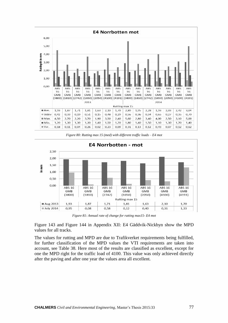
CHALMERS Civil and Environmental Engineering, Master’s Thesis 2015:33 77
Figure 80: Rutting max 15 (med) with different traffic loads – E4 mot
Figure 81: Annual rate of change for rutting max15- E4 mot
Figure 143 and Figure 144 in Appendix XII: E4 Gäddvik-Nickbyn show the MPD
values for all tracks.
The values for rutting and MPD are due to Trafikverket requirements being fulfilled,
for further classification of the MPD values the VTI requirements are taken into
account, see Table 38. Here most of the results are classified as excellent, except for
one the MPD right for the traffic load of 4100. This value was only achieved directly
after the paving and after one year the values area all excellent.

CHALMERS, Civil and Environmental Engineering, Master’s Thesis 2015:33 78
Table 38: Classifications for MPD following VTI (mot)
ABS 16
GMB
(3800)
ABS 16
GMB
(1810)
ABS 16
GMB
(2742)
ABS 16
GMB
(2050)
ABS 16
GMB
(4100)
ABS 16
GMB
(4191)
MPD
left
2013 Excellent Excellent Excellent Excellent Excellent Excellent
2014 Excellent Excellent Excellent Excellent Excellent Excellent
MPD
middle
2013 Excellent Excellent Excellent Excellent Excellent Excellent
2014 Excellent Excellent Excellent Excellent Excellent Excellent
MPD
right
2013 Excellent Excellent Excellent Excellent Bad Excellent
2014 Excellent Excellent Excellent Excellent Excellent Excellent
Table 39 shows the performance of the tracks, when comparing the reference track and
GMB with the same traffic load the reference track shows much higher life time.
However, when only comparing the GMB depending on traffic, the ones with the lowest
amount of traffic show a better performance. This could also be due to only one
available measurement.
Table 39: Current state and classification for E4 Gäddvik- Nickbyn mot, according to VTI and Trafikverket
Section Trafikverket Years to next
maintenance Rutting MPD
ABS Pt 1 (4012) Yes Yes 129
GMB (4100) Yes Yes 41
GMB (4191) Yes Yes 8,77
GMB (3800) Yes Yes 12,7
GMB (2742) Yes Yes 21,4
GMB (2050) Yes Yes 31,5
GMB (1810) Yes Yes 186,5

CHALMERS Civil and Environmental Engineering, Master’s Thesis 2015:33 79
4.5 Result overview
Table 40 shows the pavement type, traffic and needed years until maintenance of all
analysed tracks. CZ is an abbreviation for climate zone.
Table 40: Result overview
C
Z
Road
no. Location Lanes
Speed
limit
[km/h]
Traffic Asphalt type Years until
maintenance
1
E4 Kropp-
Hyllinge
10
110
11734 ABS 70/100 B 7
13383 GAP 70/100 B 7
4500 ABS 70/100 B 23
4500 GAP 70/100 B 14.5
20
11734 ABS 70/100 B 28.1
13383 GAP 70/100 B 27.8
4500 ABS 70/100 B 22.9
4500 GAP 70/100 B 33.4
E6 Fredriksberg
- Lockarp
10
110
7157 ABS 70/100 B 21.6
GAP 70/100 B 24.2
19089 ABS 70/100 B 13
17064 GAP 70/100 B 29.6
20
7157 ABS 70/100 B 50.3
GAP 70/100 B 46.5
19089 ABS 70/100 B 26.2
17064 GAP 70/100 B 55
E6 Kronetorp-
Salerup
10
110
18618 ABS 70/100 B 10.3
GAP 70/100 B 26.3
10610 ABS 70/100 B 9.7
10000 GAP 70/100 B 23.8
20
18618 ABS 70/100 B 40.4
GAP 70/100 B 26.1
10610 ABS 70/100 B 26.4
10000 GAP 70/100 B 26.4
E6
Petersborg-
Vellinge
South
10
110
17132 ABS 70/100 B 13.8
GAP 70/100 B 14.8
20 17132 ABS 70/100 B 29.2
GAP 70/100 B 36.8
E6 Sunnanå-
Kronetorp
10
110
17012 ABS 70/100 B 6.6
18294 GAP 70/100 B 26.3
20 17012 ABS 70/100 B 30
18294 GAP 70/100 B 21.6
2 E6 Ullevi-
Kallebäck
10
70
30121 ABS 70/100 PMB 9.3
GAP 70/100 B 9.5
20 30121 ABS 70/100 PMB 12.4
GAP 70/100 B 14.7

CHALMERS, Civil and Environmental Engineering, Master’s Thesis 2015:33 80
E4 Uppsala-
Knivsta
10
20 110
16971 GAP16 0.6%
Wetfix 5.0
16971 GAP16 0.6%
Wetfix Pt2 5.9
16971
GAP 16% 0.3%
Wetfix 1%
Cement
4.7
16971 GAP 16%
Increased Temp 5.5
16971 ABS 70/100 6.4
13979 ABS 50/70 7.7
13979 GAP 16 Increased
Temp Pt2 6.5
E4
Viby-
Sollentuna
Stockholm
30 110
33510 ABS 70/100 B 6.6
33510 GAP 70/100 B 6
4
E4 Broänge -
Hökmark 10 90 3800 GAP 16 100/150 15
E12 Lycksele
10
med
70 1320 ABTS 11 30
50-70 1320 ABTS 11 GMB 41
50-70 1563 ABTS 11 GMB 30
50-70 2000 ABTS 11 GMB 17,5
50-70 3361 ABTS 11 GMB 11,5
50 5600 ABTS 11 GMB 9
10
mot
70 1320 ABTS 11
50-70 1320 ABTS 11 GMB
50-70 3361 ABTS 11 GMB
E12 Storuman-
Stensele 10
50-70 1987 ABTS 16 160/220
50 1987 Gap 16
50 1987 ABTS 16 GMB 1
90 2787 ABTS 16 GMB 2
50 3040 ABTS 16 GMB 2
50 534 ABTS 16 GMB 2
5 E4 Gäddvik-
Nickbyn
10
med 110
4012 ABS 100/150
4012 Gap Pt 1
1810 Gap Pt 2
2836 Gap Pt 2
4063 Gap Pt 2
10
mot 110
4012 ABS 16 GMB
4100 ABS 16 100/150
4191 ABS 16 100/150
3800 ABS 16 100/150
2742 ABS 16 100/150
2050 ABS 16 100/150
1810 ABS 16 100/150

CHALMERS Civil and Environmental Engineering, Master’s Thesis 2015:33 81
5 Discussion
The discussions were made for each track individually and then gathered together in
order to achieve an overall picture of which asphalt type is more suitable regarding
texture and rutting
E4 Kropp- Hyllinge KF10
In this section the lifetime was equal for both the GAP and the ABS, despite more traffic
on the GAP. From it can be concluded that the GAP is more resistant to rutting than
ABS. On the section with 4500 vehicles per day the ABS lasts 8.5 years longer than the
GAP, meaning it is better suited for this section and traffic volume. The texture for the
standard asphalt is better in both sections.
On this road the use of standard ABS is recommended more regarding rut resistance
and texture. Additional measurements are recommended, since the long- term use of
GAP has not been evaluated yet.
E4 Kropp- Hyllinge KF20
In this section the ABS has a longer lifetime than the GAP at the high traffic volumes.
However, the results would need further consideration since the traffic volumes are not
equal. On the section with 4500 vehicles per day the GAP lasts 10.5 years longer than
the ABS and is clearly better suited for this road with this traffic volume. The texture
was excellent for both, nevertheless higher for ABS.
E6 Fredriksberg- Lockarp KF10 mot
The calculation showed that the GAP provides a longer lifetime at both traffic volumes.
In the section with lower traffic further measurements are necessary for a clearer result.
To judge from the annual changes the wearing varies for each year.
The rubber modified asphalt provided even a better texture and at the higher traffic the
ABS was even rated as bad by the VTI classification. This could however be related to
the higher traffic, which was more by over 2000 vehicles per day on the ABS section.
Both types fulfil Trafikverket’s requirements.
E6 Fredriksberg- Lockarp KF20 mot
All sections fulfilled Trafikverket’s requirements for maximum rut depth and texture.
Compared to the VTI requirements all types have an excellent texture. Judging by the
values the GAP provides a slightly better texture. On the section with ABS at 19089
vehicles per day the texture is lowest compared to the others, which may depend on the
high traffic volume.
E6 Kronetorp- Salerup KF10 mot
The GAP fulfilled Trafikverket’s and VTI’s requirements for rut depth and texture at
both traffic volumes. The ABS on the other hand fulfilled Trafikverket’s requirements,
but had a bad texture according to VTI. The rut depths were much higher for the ABS
and is expected to last 16 years less than the GAP at 18618 vehicles per day and 14
years less at 10000 vehicles per day.

CHALMERS, Civil and Environmental Engineering, Master’s Thesis 2015:33 82
Another observation is that the rut depth is higher for the GAP at lower traffic volumes.
The reason for this could be related to the use of less resistant aggregates on sections
with lower traffic volumes.
E6 Kronetorp- Salerup KF20 mot
The results for this lane differ from the first lane. On the sections with 10000 vehicles
per day the remaining time before maintenance is the same for both types. Since the
traffic for the ABS is 10610 vehicles per day, i.e. slightly higher than for the GAP, one
can say that the ABS is better on this section. At the section with 18618 vehicles per
day the ABS clearly has a greater advantage with an almost 14 years longer lifetime. In
terms of texture the GAP provides a better texture and in addition to this all sections
fulfil Trafikverket and VTI’s requirements.
E6 Petersborg- Vellinge KF10 mot
On this road the rubber modified asphalt has proven to provide better resistance against
rutting and a better texture than the ABS. The GAP is expected to last 1 year longer
than the standard asphalt. Weather this is an advantage sufficient enough to compensate
for the additional cost is something that still has to be investigated. Both types fulfil
Trafikverket’s requirements and are rated as excellent according to VTI’s requirements.
E6 Petersborg- Vellinge KF20 mot
On the second lane the results resemble the ones in the first lane. The GAP provides
better texture and rut resistance here as well. The GAP is expected to last for more than
seven years longer than the ABS. Both types fulfil Trafikverket’s requirements and are
rated as excellent by VTI.
E6 Sunnanå- Kronetorp KF10 med
From 2009 until 2014 the rut depth for rubber-modified asphalt increased with 2.80
mm. After the same time period the standard asphalt’s rut depth was 7.41 mm in 2011.
The difference between the two materials’ rut depth is 4.61 mm, which is almost double
the rut depth for the GAP. Considering rutting, the rubber modified asphalt would last
20 years longer than the standard asphalt, or 17 years if the paving date is taken into
consideration.
Considering texture, the better values are associated with the GAP, although the traffic
is higher on that section. On the other hand the ABS has been placed three years
previously, meaning that it has been exposed for wearing for a longer period. The rate
of change indicates that the ABS has decreased by less than 0.03 mm per year, which
could indicate that the MPD for the ABS has been low from the beginning. Both types
have an excellent texture according to classification by VTI, except for the left MPD
on the ABS, which is lower than the limit. Both fulfil Trafikverket’s requirements as
well.
E6 Sunnanå- Kronetorp KF20 med
On this lane the standard asphalt provides the better material in terms of rutting. The
ABS lasts more than eight years longer than the GAP. Considering texture the rubber
asphalt provides a better surface, despite the higher traffic. One explanation for the low
texture on the ABS could be that it was placed three years earlier. To be more certain,
additional measurements are necessary and time should pass in order to show which

CHALMERS Civil and Environmental Engineering, Master’s Thesis 2015:33 83
type lasts longer since deterioration changes with time. Both fulfil Trafikverket’s
requirements and have an excellent texture according to the VTI rating.
E6 Ullevi- Kallebäck KF10 & 20
On the first lane of the E6 in Gothenburg the measured data was very similar for both
asphalt types. The GAP had a slightly longer life span (by 0.2 years) than the PMB. On
the second lane the difference was clearer, where the rubber modified asphalt indicated
grater resistance against rutting on an average (3 years longer lifetime). The annual
increases in Figure 47 and Figure 48 have a high variation from year to year, which
does not provide an accurate representation of the pavement’s behaviour. There is no
clear picture of how the asphalt types will behave with time, hence further
measurements are needed in order to determine the better suited asphalt type for this
road.
Considering MPD no significant differences were observed in the comparison between
GAP and PMB in lane 1. For lane 1 the MPD values are between 0.55- 0.91 mm for
both types. These values fulfil Trafikverket’s requirements for texture larger than 0,35
mm at 70 km/h. Larger differences were indicated in lane 2 as the MPD value was much
higher for the PMB. Even these values fulfil Trafikverket’s requirements and are on an
average classified as acceptable by VTI.
E 47 Falköping
VTI uses advanced techniques and equipment and closes down the road in order to
achieve very precise measurements. For PMSV3 on the other hand the data is collected
with a single reading with the laser-equipped car. These differences show in the results
with a large variation up to 50% at certain instances. However, regarding the expense
in the measuring procedure and that most of the readings from PMSV3 differed by
±18% from VTI’s measurements it is possible to conclude that PMSV3 is a feasible
tool for road surveys. Since rutting is measured in millimetres it is acceptable to have a
difference of 18%, which otherwise may appear to be a high value. The VTI survey is
more suited for researchers or if certain properties of an asphalt type/mixture are
requested.
As well as being in agreement with the rutting reference tracks 1 and 2 as well as track
2 (which had the lowest rutting), they also appear to have the highest values for texture.
According to the values and the patterns there is a correlation between texture and
wearing on these asphalt types. The asphalt types with good wear resistance offer a
better texture as well. All sections had higher texture than recommended by both
Trafikverket and VTI which in other words means the asphalt types offer a skid
resistance which is too high. This affects the noise emission and fuel consumption,
which increase with too high texture.
Considering lifetime the second reference track offers the best quality by far. From an
economical point of view this asphalt type is the most recommended one.
E4 Uppsala- Knivsta
Evaluation of PMSV3 in comparison to Objektsmätning (Rutting)
The results indicated differences between the two road surveys, regarding rut depths.
On average the data from PMSV3 deviated by ±7% from the data in Objektsmätning,
which is a very acceptable range regarding the expense in the survey method and
equipment. Bearing in mind that the measured values are in millimetres, ±7% is a very

CHALMERS, Civil and Environmental Engineering, Master’s Thesis 2015:33 84
small difference and affects the outcome to a small extent. Many aspects can influence
the measurements such as equipment, driving style, traffic and most important in that
case the different occasions.
The most important factor for differences is the different measuring occasions. While
the Objektsmätning was implemented during spring and autumn, the measurements for
PMSV3 were implemented in summer meaning that the surveys were done either before
or after Objektsmätning. Considering that most of the deformation occurs during winter
time, this time difference has a minor influence on the measurements.
These differences however affected the results when comparing the rutting caused in
winter with the rutting during the whole year. In the calculations almost all
measurements were larger for the winter period to a small degree, which is not logical.
One explanation for why the results are differing is the difference in the measuring
methods. Moreover the small difference indicates that most of the wearing is caused
during the winter period by studded tires.
Conclusion
According to the measurements and results PMSV3 is a feasible analysis tool. In
general there is one drawback with PMSV3, which is the extra editing work in the data
files before the data can be used for analysis.
Comparison of GAP to ABS
Texture
There is a clear difference in texture (MPD) between GAP and ABS. The texture in the
sections with modified asphalt was much higher than the texture for the standard
asphalt. On the GAP sections the MPD values were all above 1 mm during the period
between 2011 and 2014, while MPD on the reference sections was below 1 mm.
Furthermore, the rate of change was higher for the reference sections, meaning the
texture decreased faster.
Rutting
On the test road the rubber modified asphalt was more sensitive to rutting than the
standard asphalts. The standard types would last at least one year longer with the two
traffic volumes according to the last measurement and the average changing rate.
Conclusions
The modified asphalt is more suited for this section regarding texture since the
measured values were larger than the reference track and decreased slower. Therefore
it is possible to conclude that the texture on GAP is more stable and does not change
extremely. The standard ABS on the other hand is more resistant to wearing by studded
tyres, which results in less rutting.
Wearing per 1 million wheel passages
The wearing which was calculated for one million wheel passages enables the
comparison between asphalt types independent of traffic volumes. In this calculation
the number of cars was neutralized. The effect of this neutralization becomes clear
when the values are compared to the results in Figure 56 and Figure 57. In these figures
tracks 3 and 4 have the greatest rutting, however in Figure 58 the last track has the
largest rutting, which only became clear when the traffic amount was neutralized.

CHALMERS Civil and Environmental Engineering, Master’s Thesis 2015:33 85
Texture change per 1 million wheel passages
The results in Figure 59 indicate that the texture for GAP increases, while it decreases
for the ABS. As long as the values are within the required range there is no large
difference between increase and decrease. The values matter when they become
extreme, which may indicate the wearing of the aggregates if the MPD decreases, and
the loss of aggregates if the MPD increases.
In order to verify in which direction the texture is moving it is possible to compare it to
the MPDs in Figure 127, Figure 128 and Figure 129 in Appendix VIII: E4 Uppsala-
Knivsta. In these figures the textures behave in the same way they did in Figure 59.
They decrease for the reference track and increase for the modified tracks. The
following years it starts to decrease for all sections in different degrees. The tracks are
still within the recommendations from Trafikverket according to Figure 127, Figure
128 and Figure 129 in Appendix VIII: E4 Uppsala-Knivsta, hence no judgment can be
made with the present data and further measurements are needed.
The data however provides a hint in which direction the asphalt types are going and in
what way the deterioration occurs. In this case the aggregates in the standard asphalt
seem to be worn out and crushed, while they would loosen and fall out in the rubber
modified asphalt.
Conclusions
Transforming the wearing to a neutral number independent of traffic enables the
comparison of asphalt types in sections with different traffic volumes. In our opinion
this number is an effective way of evaluating wearing on a road.
E4 Viby- Sollentuna (Stockholm) KF30 mot
The results in Table 26 imply that the ABS is more resistant to rutting than the GAP
and that it is better suited for this section on the road. In terms of texture the rubber
modified asphalt was better. On the other hand, there were too few measurements on
this road. Data from three years’ worth of measurements are not enough data to base a
decision on.
E4 Broänge-Hökmark K10 med
In this case the Gap meets the requirements of Trafikverket and is classified as excellent
for all three measurements for approximately 3800 cars per day and 90 km/h. However
due to the incorrectly registered data it is unsure if these values are correct and a
reference track was missing for comparison.
E12 Lycksele K10 med
For the med direction the reference track shows worse results for rutting than the GMB
even with lower traffic load. The track would need maintenance 10 years before the
GMB track. However the texture for the reference track is better classified than for the
GMB.
For the PMSV3, the correct data regarding pavement type and pavement date should
be registered correctly. The modified asphalt could not be found only using the search
function in PMSV3 and no further information.
Additional measurements are recommended, since the long- term use of GMB has not
been evaluated yet.

CHALMERS, Civil and Environmental Engineering, Master’s Thesis 2015:33 86
E12 Lycksele K10 mot
For the mot direction the reference track shows lower values after the first month of
pavement, however during the first year the initial rutting is higher in total for the
reference track than for the GMB.
On the reference track the texture ranks higher in the classification than the GMB.
Additional measurements are recommended since the long- term use of GMB could not
be evaluated with the present amount of data.
E12 Storuman- Stensele K10 med
Here three different pavements could be compared. After the first year the reference
track followed by the GMB show the best results. However in the following two years
the GAP has a lower annual change than the GMB.
For the texture the reference track is classified worst and GMB best. However, for all
three pavements the right side is classified as bad.
For texture and rutting additional measurements are recommended, since the long term
use of GAP and GMB could not been evaluated yet.
Furthermore, for the PMSV3 the correct data regarding pavement type and pavement
date should be registered correctly. The modified asphalt could not be found only using
the search function in PMSV3 or without additional information.
E4 Gäddvik-Nickbyn K10 med and mot
For the med direction the rut depth values vary in some parts more than others and
therefore have a higher range of values concluding in higher average values with similar
traffic load.
While comparing the reference and Gap track, the reference track shows better results
for initial rutting.
For the texture, the classification is excellent according to VTI, it must be mentioned
that the classification ranges are only for speed limit up to 100 km/h, however for this
track the speed limit is 110 km/h. Therefore the classification might be only good for
an overview and not for an actual classification.
For texture and rutting additional measurements are recommended since the long- term
use could not be evaluated yet.
For PMSV3 again it is important to register the pavements correctly due to
misunderstandings if no additional data is provided. In this case, data from the
construction company was available and it was therefore known that no additional
reference track was paved in mot direction.

CHALMERS Civil and Environmental Engineering, Master’s Thesis 2015:33 87
6 Conclusions and future recommendations
During the analysis of the measured data several observations were made regarding
asphalt types, deformation patterns and the use of PMSV3. We expected the RMA to
be more resistant to rutting than our results showed, since the studies from Arizona
clearly promised better performance. The different outcome can mainly be related to
the use of studded tires in Sweden and difference in climate.
The use of PMSV3 for our analysis was helpful. It was both easy to use and
straightforward and provided a high amount of useful data, not only about rut depth and
texture but also about traffic, prognoses, statistics and many other parameters. The
system has the advantage that information on each road is provided with pictures and
graphs and can be changed directly during use, besides the map that shows the current
location. Another advantage is its price efficiency compared to surveys from VTI which
can be three to five times the price of analysis with PMSV3.
There were a few disadvantages as well, such as incorrect reporting in the data base
about pavement type. For some roads there was no information about the pavement
type or it did not correspond to the information provided by the contractors. The same
problem applies to the coordinates for a few sections. Finally, the data editing is time
consuming, especially when there are many different asphalt types and many different
traffic volumes.
Rubber modified asphalt
The evaluation of rubber modified asphalt could have been more comprehensive, if all
information had been available in PMSV3. Most of the tracks that provided data from
many years for a good comparison were located in climate zone 1. In climate zone 2
the available data was limited and no conclusion for which asphalt type is better could
be made. For instance, the E6 in Gothenburg was compared to ABS with PMB, not the
standard binder. Other roads are the E18 and E20 in Örebro, where many different
products can be found as it was in Uppsala. The data from these roads would have been
an important aspect for our comparison; however it was left out since the road was
placed recently and no data was available in PMSV3. These tracks are however good
examples for this kind of analysis in the future.
The surface properties for the GAP showed an increased rut resistance and higher
texture than conventional asphalt, especially in climate zone 1. On the E6 in
Fredriksberg the lifetime of the rubber modified asphalt was up to 29 years longer than
the conventional asphalt. On the E6 in Gothenburg, located in climate zone 2 it
performed better than polymer modified asphalt, which is supposed to be a better option
than conventional asphalt. In Uppsala and Stockholm on the other hand the standard
asphalt only provided better rut resistance. For climate zone 2 it is therefore not clear
which asphalt type performs better and more measurements are necessary in the future.
In the north the provided data was insufficient for a conclusion. Most tracks were
measured only once so would make a good starting point for future studies.
As a last step the wearing for one million wheel passages was calculated, which enabled
the comparison for wearing independent of traffic. This number is very useful for roads
with different traffic volumes and asphalt types. This calculation was applied on the E4
in Uppsala and verified that the GAP was more sensitive to wearing there.

CHALMERS, Civil and Environmental Engineering, Master’s Thesis 2015:33 88
Future recommendations
A clearer reporting of pavement data regarding type and start and stop coordinates
would facilitate the work on a large scale. PMSV3 is a very suitable tool for road
surveys and recommended for future use regarding accuracy and cost. Rubber modified
asphalt has a great potential and could compensate for the extra cost of 20% with longer
lifetime. However, additional measurements are necessary to evaluate GAP for a long
term perspective.

CHALMERS Civil and Environmental Engineering, Master’s Thesis 2015:33 89
7 References
ASTM International, 2011. Standard Test Method for Measuring Rut-Depth of
Pavement Surfaces using a Straightedge, Pennsylvania US: ASTM International.
Amirkhanian, S., 2013. Overview of Rubberized Asphalt Technology. Las Vegas:
Environmental Protection Agency.
Andersson, P., 2008. Technical Description of Flow- Mixed Asphalt- KGO-III. 2008:95
ed. Borlänge: Trafikverket.
APAI, n.d.. Asphalt Paving Design guide. West Des Moines, US: Asphalt Paving
Association of Iowa.
Asfaltskolan, n.d.. Detta är asfalt. [Online] Available at:
http://www.asfaltskolan.se/Allmantomasfalt.htm [Accessed February 2015].
Asfaltskolan, n.d. Asfaltskolan. [Online] Available at:
http://www.asfaltboken.nu/inside/frameset.asp [Accessed February 2015].
Auto Vina, 2012. AutoVina. [Online] Available at: http://autovina.com/article/dai-lo-
dong-tay-doan-duong-nguy-hiem-6650.html [Accessed 04 May 2015].
Bast, 2010. Bundesanstalt für Straßenwesen. [Online] Available at:
http://www.bast.de/DE/FB-S/Technik/FWD.pdf?__blob=publicationFile [Accessed 05
May 2015].
Bieder, A. & Jenzer , L., 2011. Measurement of the softening point using the ring-and-
ball test in the CRD Laboratory, Langenthal: Ammann Group.
Carlson, D. D. & Zhu, H., 1999. Asphalt- Rubber An Anchor to Crumb Rubber Markets,
Veracruz, Mexico: International Rubber Forum.
City of Mankano, n.d. Seal coat program. [Online] Available at: http://www.mankato-
mn.gov/Streets-Seal-Coat/Page.aspx [Accessed February 2015].
Civil Engineering Portal, n.d.. Sieve Analysis of Aggregates. [Online] Available at:
http://www.engineeringcivil.com/sieve-analysis.html [Accessed 19 May 2015].
Clemson University, 2002. Asphalt rubber Technology Service. [Online] Available at:
http://www.clemson.edu/ces/arts/glossary.html [Accessed February 2015].
Controls Group, n.d.. Bar sieves (Grids). [Online] Available at: http://www.controls-
group.com/eng/aggregates-testing-equipment/bar-sieves-grids.php [Accessed 04 May
2015].
Darabian, F., 2015. Project management system. Gothenburg: Trafikverket.
Dr Read, J. & Whiteoak, D., 2003. The shell Bitumen Handbook. 5th ed. UK: Shell UK
Oil Products Limited.
ecore Athletic, n.d.. Exposure to crumb rubber products poses no risk to adult, children
or pets. [Online] Available at: http://ecoreathletic.com/Sustainability/Rubber-Crumb-
Facts [Accessed 27 May 2015].
EMPA, n.d.. Pavement Performance and In-situ testing. [Online] Available at:
http://www.empa.ch/plugin/template/empa/797/*/---/l=2 [Accessed 10 May 2015].
EPA, 1995. AP 42, Fifth edition Compilation of Air Pollutant Emission Factors,
Volume 1: Stationary Point and Area Sources, North Carolina: Research Triangle Park.

CHALMERS, Civil and Environmental Engineering, Master’s Thesis 2015:33 90
EPG, 2007. Batch Component. [Online] Available at:
http://epg.modot.org/index.php?title=Image:460.3.1.1_batch_component.jpg
[Accessed 3 March 2015].
FHWA, 2012. User Guidelines for Waste and Byproduct Materials in Pavement
Construction. [Online] Available at:
http://www.fhwa.dot.gov/publications/research/infrastructure/structures/97148/st2.cf
m [Accessed 30 January 2015].
Haseeb, J., n.d.. Civil Engineering Dictionary. [Online] Available at:
http://www.aboutcivil.org/to-perform-los-angeles-abrasion-test.html [Accessed 03
May 2015].
Heitzman, M., 1992. Design and Construction of Asphalt Paving Materials with Crumb
Rubber Modifier, Washington D.C.: U.S. Department of Transportation- Federal
Highway Administration.
HNA, 2012. Rückgewinnung: Aus Altreifen wird bei der Pyrolyse zum Beispiel ein
Gummigranulat gewonnen. In Homberg könnte eine Pyrolyse-Anlage entstehen..
[Online] Available at: http://www.hna.de/lokales/fritzlar-homberg/maximal-
arbeitsplaetze-2433591.html [Accessed 27 May 2015].
Huang, Y. H., 2003. Pavement analysis and design. 2nd ed. Michigan: Prentice Hall.
Iowa State University, 2015. Institute for Transportation. [Online] Available at:
http://www.ceer.iastate.edu/facilities/plt/ [Accessed 03 May 2015].
Karlsson, H., 2015. Profilmätning på Sträckor med polymermodifierat bitumen på
riksväg 47 Falköping, Linköping: VTI.
Kenenth Lind, 2012. Trafikverket: Abrasion by studded tyres (Prall-value). [Online]
Available at: http://www.nordfou.org/documents/prall/projektlederseminar_prall.pdf
[Accessed 19 May 2015].
Kim, H. B., Lee, S. W., Hyun, H.-S. & Lee, K. H., 2013. Measurement of Texture
Depth of Pavement Using Potable Laser Profile. Proceeding of the Eastern Asia Society
for Transportation Studies Vol. 9.
Lo Presti, D., Airey, G. & Partal, P., 2012. Manufacturing terminal and field bitumen-
tyre rubber blends: the importance of processing conditions. Nottingham, Elsevier Ltd.
Selection, pp. 458-494.
Lund University , 2014. Road Construction- Labratory Instructions, Lund: Lund
University Department of Engineering, Institution for Technique and Society.
Lundberg, T., Sjögren, L., Gustafsson, M. & Ihs, A., 2011. Vägytans makrotextur och
dess variation, Linköping: VTI.
Matest, n.d.. Marshall/CBR Compression frames for bituminous specimens. [Online]
Available at: http://matest.com/en/Products/bitumen-asphalt/MARSHALL-TESTING-
MACHINES-AND-BATHS-/marshallcbr-compression-frames-for-bituminous-
specimens [Accessed 23 May 2015].
Mellela, R. & Wang, H., 2006. Harmonising Automated Rut Depth Measurements-
Stage 2, Wellington: Land Transport New Zealand Research Report 277.
Ministry of Transportation, Ontario, 2001. Labratory Testing Manual: Method of test
for the determination of indirect tensile strength of expanded asphalt mixes, Ontario:
Ministry of Transportation.

CHALMERS Civil and Environmental Engineering, Master’s Thesis 2015:33 91
Nordgren, T., 2014. Handledning för tillverkning av asfaltmassa/beläggning inom FOI-
upphandling med gummi modifierat bitumen 2015, Borlänge: Trafikverket.
Nordgren, T., 2015. Asphalt [Interview] (March 2015).
Nordgren, T. & Tykesson, A., 2011. Dense graded Asphalt rubber in cold climate
conditions, Göteborg: Trafikverket.
O'Flaherty, C. A., 2002. Highways 4 th Edition. Oxford: Butterworth-Heinemann.
Parhamifar, E., 2014. Asphalt Lecture 3rd September 2014. Göteborg: Lund University.
Pavement Interactive, 2010. Maintenance and Rehabilitation. [Online] Available at:
http://www.pavementinteractive.org/article/bituminous-surface-treatments/ [Accessed
03 May 2015].
Persson, K., 2014. Bitumen- Properties and Testing Lecture 10th September 2014.
Göteborg: Total Nordic.
Petro Asian FZC, n.d. PA Petro Asian FZC. [Online] Available at:
http://petroasianfzc.com/OurProducts.php [Accessed 04 May 2015].
Queensland Government, 2009. MRTS30 Dense Graded and Open Graded Asphalt,
Queensland: Department of Transport and Main Roads.
Roadway Inventory & Testing Section (RITS), 2005. Pennsylvania Department of
Transportation. [Online] Available at:
http://www.dot.state.pa.us/Internet/Bureaus/pdBOMO.nsf/DivRoadInventory?OpenFr
ameset [Accessed 05 May 2015].
RuBind inc., n.d.. RuBind inc. elastomeric asphalt extender. [Online] Available at:
http://rubind.com/index.php?id_cat=5&p=page [Accessed 27 May 2015].
Subadra Consulting Ltd, n.d.. Subadra Consulting Ltd. [Online] Available at:
http://www.subadra.com/geotechnical/cbr-and-plate-bearing-tests/ [Accessed 03 May
2015].
Tariq, U., 2013. Slideshare. [Online] Available at:
http://www.slideshare.net/UmairTariq10/open-graded-friction-course-ogfc [Accessed
3 February 2015].
Test International, 2014. Nordic Abrasion Machine. [Online] Available at:
http://testinternational.co.uk/aggregate-testing/nordic-abrasion-machine.php
[Accessed 03 May 2015].
Trafikverket PMSV3, 2015. PMSV3 Analysera Strecka, Borlänge: Trafikverket.
Trafikverket Underhållsstandard, 2012. Underhållsstandard belagd väg 2011,
Borlänge: Trafikverket.
Trafikverket, 2005. ATB Väg 2005 Kapitel F Bitumenbundna lager, Borlänge:
Trafikverket.
Trafikverket, 2014. Användarmanual PMSV3- Information om belagda vägar. 1.2.2 ed.
Borlänge: Trafikverket.
Trafikverket, 2015. Trafikflödeskartan. [Online] Available at:
http://vtf.trafikverket.se/SeTrafikinformation# [Accessed 1 April 2015].

CHALMERS, Civil and Environmental Engineering, Master’s Thesis 2015:33 92
Vanseenkiste, S. et al., 2008. Validation of the indirect tensile strength ratio (ITSR) as
a performance indicator for water sensitivity of asphalt pavements, Copenhagen:
European Asphalt Pavement Association.
Way, George, 2012. History of Asphalt Rubber in Arizona. Tempe, Arizona,
Consulpav.
Way, G. B., Kaloush, K. E. & Biligiri, K. P., 2011. Asphalt- Rubber Standard Practice
Guide, Arizona: Rubber Pavement Association.
Werner Corporation, n.d. Asphalt Maintenance Aggregates. [Online] Available at:
http://www.wernercorp.net/asphalt-maintenance-aggregates/ [Accessed 04 May 2015].
Vägverket, 2004. Allmän teknisk beskrivning för vägkonstruktion - ATB Väg 2004 -
Kapitel A Gemensamma förutsättningar, Borlänge: Vägverket.
Yildirim, Y., 2005. Polymer modified asphalt binders , Austin, Texas: Department of
Civil Engineering, University of Texas at Austin.

CHALMERS Civil and Environmental Engineering, Master’s Thesis 2015:33 93
8 List of figures
Figure 1: Different sizes of aggregates (Werner Corporation, n.d.) ............................ 3
Figure 2: Aggregates covered in bitumen (Petro Asian FZC, n.d) .............................. 4
Figure 3: Schematic design SAM & SAMI (Way, George, 2012) .............................. 6
Figure 4: Chip seal coating. Spreading out aggregates on hot asphalt- rubber liquid (City
of Mankano, n.d) ....................................................................................................... 6
Figure 5: Aggregate structure in dense-, gap- and open graded asphalts (Tariq, 2013) 8
Figure 6: Dense graded asphalt mix (Way, George, 2012) ......................................... 9
Figure 7: Aggregate content in open graded asphalt mix (Way, George, 2012) .......... 9
Figure 8: Batch Mix Plant (EPG, 2007) ................................................................... 10
Figure 9: Rubber modified bitumen- high viscosity (left) and terminal blend (right) (Lo
Presti, et al., 2012) ................................................................................................... 11
Figure 10: Extreme rutting in wheel paths (Auto Vina, 2012) .................................. 13
Figure 11: Micro-, macro-, and mega texture with respective wavelength interval as
well as irregularities after (Lundberg, et al., 2011) ................................................... 14
Figure 12: Bleeding in the wheel paths (Pavement Interactive, 2010) ...................... 15
Figure 13: Bar sieves for flakiness index (Controls Group, n.d.) .............................. 16
Figure 14: Ring and Ball method (Bieder & Jenzer , 2011) ...................................... 17
Figure 15: Marshall/ CBR Compression (Matest, n.d.) ............................................ 17
Figure 16: Tools for Accelerated Pavement Testing (EMPA, n.d.) ........................... 19
Figure 17: Test equipment and sketch (Lind, 2012) ................................................. 19
Figure 18: Hydraulic Jack for plate bearing capactity measurement (Iowa State
University, 2015) ..................................................................................................... 20
Figure 19: Sketch of FWD principal (Bast, 2010) .................................................... 20
Figure 20: Rut measurement ( ASTM International, 2011) ...................................... 21
Figure 21: Multilaser/ Profilometer laser positioning (Mellela & Wang, 2006) ........ 21
Figure 22: Sand Patch Test (Kim, et al., 2013) ......................................................... 22
Figure 23: Systems in Trafikverket's working routines after (Darabian, 2015) ......... 23
Figure 24: Laser profile meters (Karlsson, 2015) ..................................................... 24
Figure 25: Profile cross section measurement with Primal (Karlsson, 2015) ............ 25
Figure 26: Climate zones 1 to 5 in Sweden (Vägverket, 2004) ................................. 28
Figure 27: E4 Kropp- Hyllinge, 15870- 20415 (Trafikverket PMSV3, 2015) ........... 30
Figure 28: Average values and Standard deviation of rutting on GAP and ABS, high
traffic volumes ........................................................................................................ 31
Figure 29: Average values and standard deviation of rutting on GAP and ABS, low
traffic volume .......................................................................................................... 31

CHALMERS, Civil and Environmental Engineering, Master’s Thesis 2015:33 94
Figure 30: Average values and annual change for rutting on standard ABS and GAP
................................................................................................................................ 32
Figure 31: Average values and standard deviations for rutting, MPD left, middle and
right on ABS and GAP ............................................................................................ 33
Figure 32: Average values and rate of change for rutting on GAP and ABS ............. 33
Figure 33: E6 Fredriksberg- Lockarp, 108091- 112673 (Trafikverket PMSV3, 2015)
................................................................................................................................ 34
Figure 34: Average values and rate of change for rutting on GAP and ABS with traffic
volume of 7157 vehicles per day ............................................................................. 35
Figure 35: Average values and rate of change for rutting on GAP and ABS with traffic
volume of 17064 and 19089 vehicles per day .......................................................... 35
Figure 36: Average values and rate of change for rutting on GAP and ABS ............. 36
Figure 37: E6 Kronetorp- Salerup, 98965-105524 (Trafikverket PMSV3, 2015) ...... 37
Figure 38: Average values and rate of change for rutting on GAP and ABS ............. 38
Figure 39: Average values and rate of change for rutting on ABS and GAP ............. 39
Figure 40: E6 Petersborg- Vellinge, 115947-125955 (Trafikverket PMSV3, 2015) .. 40
Figure 41: Average values and rate of change for rutting on GAP and ABS ............. 41
Figure 42: Average values and rate of change for rutting on GAP and ABS ............. 42
Figure 43: E6 Sunnanå- Kronetorp, 36016-41005 (Trafikverket PMSV3, 2015) ...... 43
Figure 44: Average values and rate of change for rutting on GAP and ABS ............. 43
Figure 45: Average values and rate of change for rutting on GAP and ABS ............. 44
Figure 46: E6 Ullevi- Kallebäck, 176896-179689 (Trafikverket PMSV3, 2015) ...... 45
Figure 47: Average value and annual change for rutting on PMB and GAP, lane 1 .. 46
Figure 48: Average value and annual change for rutting on PMB and GAP, lane 2 .. 47
Figure 49: RV47 Falköping, 21220-23720 (Trafikverket PMSV3, 2015) ................. 48
Figure 50: Average rut depth for test track on RV47, Falköping- PMSV3 ................ 49
Figure 51: Annual increase of rut depth for test track on RV47, Falköping- PMSV3 49
Figure 52: Average value for rut depth for each section 2011, 2012 and 2013 (Karlsson,
2015) ....................................................................................................................... 50
Figure 53: Rut depth increase from 2011- 2012 and 2012- 2013 for each track
(Karlsson, 2015) ...................................................................................................... 50
Figure 54: E4 Uppsala- Knivsta, 84720-101329 (Trafikverket PMSV3, 2015) ......... 52
Figure 55: Average values and annual increase of rut depth on Tracks 1, 2 and
Reference track 70/100 at 16971 vehicles/day ......................................................... 53
Figure 56: Average values and annual increase of rut depth on Tracks 3, 4 and
Reference track 70/100 at 16971 vehicles/day ......................................................... 54
Figure 57: Average values and annual increase of rut depth on Track 5 and reference
track 70/100 at 13979 vehicles/day .......................................................................... 54

CHALMERS Civil and Environmental Engineering, Master’s Thesis 2015:33 95
Figure 58: Wear of studded tyres caused by 1million wheel passages during winter
2011/2012, lane 1 .................................................................................................... 57
Figure 59: Texture change during the winter 2011/2012, E4 Uppsala KF10 ............. 58
Figure 60: E4 Viby- Sollentuna, 27317-30873 (Trafikverket PMSV3, 2015) ........... 59
Figure 61: Average values and rate of change for rutting on GAP and ABS ............. 59
Figure 62: Mångbyn E4 156720 to 164260 (Trafikverket PMSV3, 2015) ................ 61
Figure 63: PMSV3 history graph and rutting max 15 for E4 med track 156720 to 164260
................................................................................................................................ 62
Figure 64: E4 Broänge- Hökmark - Annual change for MPD and Rutting ................ 63
Figure 65: Lycksele med direction 151932 to 158798 (Trafikverket PMSV3, 2015) 64
Figure 66: Rutting Max 15 and acceptable level of 4 mm from PMSV3 ................... 65
Figure 67: Rutting Max 15 and acceptable level of 4 mm from Destia ..................... 65
Figure 68: Rutting max 15 (med) for ABTS11 with GMB and different traffic load 66
Figure 69: Rutting max15 for ABTS11 reference track and ABTS 11 with GMB .... 66
Figure 70: Rutting max 15- annual rate of change for ABTS11 reference track and
ABTS 11 with GMB ................................................................................................ 67
Figure 71: Lycksele mot 307155 to 309235 (Trafikverket PMSV3, 2015) ............... 68
Figure 72: Annual rate of change mot ...................................................................... 69
Figure 73: Stensele to Storuman 252081 to 259558. (Trafikverket PMSV3, 2015) ... 70
Figure 74: Rutting max 15 (med) with different traffic loads ................................... 71
Figure 75: Annual rate of change for rutting max15 ................................................. 71
Figure 76: E4 Gäddvik to Nickbyn 72798 to 89450 (Trafikverket PMSV3, 2015) ... 73
Figure 77: Rutting max 15 (med) with different traffic loads – E4 med .................... 74
Figure 78: Annual rate of change for rutting max15- E4 med ................................... 74
Figure 79: Pavement history for track 112038 to 130608, Norrbotten E4 ................. 76
Figure 80: Rutting max 15 (med) with different traffic loads – E4 mot .................... 77
Figure 81: Annual rate of change for rutting max15- E4 mot ................................... 77
Figure 82: Average values for rutting, MPD left, middle and right between 2010 and
2014 .......................................................................................................................101
Figure 83: Average values for rutting, MPD left, middle and right between 2010 and
2014 .......................................................................................................................101
Figure 84: Average values and annual change for MPD left for standard ABS and GAP
...............................................................................................................................102
Figure 85: Average values and annual change for MPD middle for standard ABS and
GAP .......................................................................................................................102
Figure 86: Average values and annual change for MPD right for standard ABS and
GAP .......................................................................................................................102
CHALMERS, Civil and Environmental Engineering, Master’s Thesis 2015:33 96
Figure 87: Average values for GAP and ABS along the test track, 11734 & 13383
vehicles per day ......................................................................................................103
Figure 88: Measured values for GAP and ABS along the test track, 4500 vehicles per
day .........................................................................................................................103
Figure 89: Average values and rate of change for MPD left on GAP and ABS........103
Figure 90: Average values and rate of change for MPD middle on GAP and ABS ..104
Figure 91: Average values and rate of change for MPD right on GAP and ABS .....104
Figure 92: Rutting and MPD left, middle and right with traffic volumes 17064 and
19089 vehicles per day ...........................................................................................105
Figure 93: Rutting and MPD left, middle and right with traffic volume 7157 vehicles
per day ...................................................................................................................105
Figure 94: Average values and rate of change for MPD left on GAP and ABS........106
Figure 95: Average values and rate of change for MPD middle on GAP and ABS ..106
Figure 96: Average values and rate of change for MPD right on GAP and ABS .....106
Figure 97: Average values and rate of change for MPD left on GAP and ABS........107
Figure 98: Average values and rate of change for MPD middle on GAP and ABS ..107
Figure 99: Average values and rate of change for MPD right on GAP and ABS .....107
Figure 100: Average values and rate of change for MPD left on GAP and ABS ......108
Figure 101: Average values and rate of change for MPD middle on GAP and ABS 108
Figure 102: Average values and rate of change for MPD right on GAP and ABS ...109
Figure 103: Average values and rate of change for MPD left on GAP and ABS ......109
Figure 104: Average values and rate of change for MPD middle on GAP and ABS 109
Figure 105: Average values and rate of change for MPD right on GAP and ABS ...110
Figure 106: Average values and rate of change for MPD left on GAP and ABS ......111
Figure 107: Average values and rate of change for MPD middle on GAP and ABS 111
Figure 108: Average values and rate of change for MPD right on GAP and ABS ...112
Figure 109: Average values and rate of change for MPD left on GAP and ABS ......112
Figure 110: Average values and rate of change for MPD middle on GAP and ABS 112
Figure 111: Average values and rate of change for MPD right on GAP and ABS ...113
Figure 112: Average values and rate of change for MPD left on GAP and ABS ......114
Figure 113: Average values and rate of change for MPD middle on GAP and ABS 114
Figure 114: Average values and rate of change for MPD right on GAP and ABS ...115
Figure 115: Average values and rate of change for MPD left on GAP and ABS ......115
Figure 116: Average values and rate of change for MPD middle on GAP and ABS 115
Figure 117: Average values and rate of change for MPD right on GAP and ABS ...116
Figure 118: Average value and annual change for MPD left on PMB and GAP, lane 1
...............................................................................................................................117

CHALMERS Civil and Environmental Engineering, Master’s Thesis 2015:33 97
Figure 119: Average value and annual change for MPD middle on PMB and GAP, lane
1 .............................................................................................................................117
Figure 120: Average value and annual change for MPD right on PMB and GAP, lane 1
...............................................................................................................................118
Figure 121: Average value and annual change for MPD left on PMB and GAP, lane 2
...............................................................................................................................118
Figure 122: Average value and annual change for MPD middle on PMB and GAP, lane
2 .............................................................................................................................118
Figure 123: Average value and annual change for MPD right on PMB and GAP, lane 2
...............................................................................................................................119
Figure 124: Average values for left MPD on test sections on RV 47 Falköping ......120
Figure 125: Average values for middle MPD on test sections on RV 47 Falköping .120
Figure 126: Average values for right MPD on test sections on RV 47 Falköping ....120
Figure 127: Average values and annual increase for MPD left on GAP and ABS 70/100
...............................................................................................................................121
Figure 128: Average values and annual increase for MPD middle on GAP and ABS
70/100 ....................................................................................................................121
Figure 129: Average values and annual increase for MPD right on GAP and ABS
70/100 ....................................................................................................................121
Figure 130: Average measurements for rutting on E4 in Uppsala, PMSV3 .............122
Figure 131: Average measurements for rutting on E4 in Uppsala, Objektsmätning .123
Figure 132: Measurements for rutting, MPD left, middle and right on GAP and ABS
...............................................................................................................................124
Figure 133: Average values and rate of change for MPD left on GAP and ABS ......124
Figure 134: Average values and rate of change for MPD middle on GAP and ABS 124
Figure 135: Average values and rate of change for MPD right on GAP and ABS ...125
Figure 136: MPD left and right (med) - annual rate of change for ABTS11 reference
track and ABTS 11 with GMB ...............................................................................126
Figure 137: MPD middle (med) - annual rate of change for ABTS11 reference track
and ABTS 11 with GMB ........................................................................................126
Figure 138: Annual rate of change for MPD left .....................................................127
Figure 139: Annual rate of change for MPD middle ...............................................127
Figure 140: Annual rate of change for MPD right ...................................................128
Figure 141: Annual rate of change for MPD left and right- E4 med ........................129
Figure 142: Annual rate of change for MPD middle – E4 med ................................129
Figure 143: Annual rate of change for MPD left and right- E4 mot .........................130
Figure 144: Annual rate of change for MPD middle – E4 mot ................................130

CHALMERS, Civil and Environmental Engineering, Master’s Thesis 2015:33 98
9 List of tables
Table 1: Testing standards for stone aggregates (Trafikverket, 2005) ....................... 25
Table 2: VTI classification of MPD with speed limits, considering texture (Lundberg,
et al., 2011) ............................................................................................................. 26
Table 3: Trafikverket requirements for MPD based on traffic volumes and speed limits
(Trafikverket Underhållsstandard, 2012) ................................................................. 26
Table 4: Trafikverket requirements for rutting based on traffic volumes and speed limits
(Trafikverket Underhållsstandard, 2012) ................................................................. 26
Table 5: List of tracks used for the investigation according to climate zone ............. 29
Table 6: Current state and classification for E4 Kropp- Hyllinge KF10 according to VTI
and Trafikverket ...................................................................................................... 32
Table 7: Current state and classification for E4 Kropp- Hyllinge KF20 med, according
to VTI and Trafikverket ........................................................................................... 34
Table 8: Current state and classification for E6 Fredriksberg- Lockarp KF10 mot,
according to VTI and Trafikverket........................................................................... 36
Table 9: Current state and classification for E6 Fredriksberg- Lockarp KF20 mot,
according to VTI and Trafikverket........................................................................... 37
Table 10: Current state and classification for E6 Kronetorp- Salerup KF10 mot,
according to VTI and Trafikverket........................................................................... 38
Table 11: Current state and classification for E6 Kronetorp- Salerup KF20 mot,
according to VTI and Trafikverket........................................................................... 39
Table 12: Current state and classification for E6 Petersborg- Vellinge KF10 mot,
according to VTI and Trafikverket........................................................................... 41
Table 13: Current state and classification for E6 Petersborg- Vellinge KF20 mot,
according to VTI and Trafikverket........................................................................... 42
Table 14: Current state and classification for E6 Sunnanå- Kronetorp KF10 med,
according to VTI and Trafikverket........................................................................... 44
Table 15: Current state and classification for E6 Sunnanå- Kronetorp KF10 med,
according to VTI and Trafikverket........................................................................... 45
Table 16: Current state and classification for E6 Ullevi- Kallebäck, KF10 and 20 med,
according to VTI and Trafikverket........................................................................... 47
Table 17: Material composition of test sections on RV47 Falköping ........................ 48
Table 18: Result comparison between data from PSMV3 and VTI........................... 51
Table 19: VTI's proposed classification of MPD with speed limits, considering friction
and aquaplaning, RV 47 Falköping .......................................................................... 51
Table 20: Sectioning of test track according to material order .................................. 52
Table 21: Comparison of test tracks with reference track 70/100, rutting ................. 55
Table 22: Comparison of test track 5 with reference track 50/70, rutting .................. 55
Table 23: Classification of E4- Uppsala according to Trafikverket and VTI ............. 55
CHALMERS Civil and Environmental Engineering, Master’s Thesis 2015:33 99
Table 24: Differences between PMSV3 and Objektsmätning for rut depths on the E4 in
Uppsala ................................................................................................................... 56
Table 25: Proportion between rutting during winter and whole year ........................ 57
Table 26: Current state and classification for E4 Stockholm, Viby- Sollentuna KF30
mot, according to VTI and Trafikverket ................................................................... 60
Table 27: Classifications for MPD following VTI ................................................... 63
Table 28: Current state and classification for E4 Broänge-Hökmark KF10 according to
VTI and Trafikverket ............................................................................................... 63
Table 29: Speed and Rutting from PMSV3 and Destia for med................................ 65
Table 30: Classifications for MPD following VTI (med) ......................................... 67
Table 31: Current state and classification for E12 Lycksele med, according to VTI and
Trafikverket ............................................................................................................ 68
Table 32: Classifications for MPD following VTI (mot) .......................................... 69
Table 33: Current state and classification for E12 Lycksele mot, according to VTI and
Trafikverket ............................................................................................................ 69
Table 34: Classifications for MPD following VTI (med) ......................................... 72
Table 35: Current state and classification for E12 Storuman-Stensele med, according to
VTI and Trafikverket ............................................................................................... 72
Table 36: Classifications for MPD following VTI (med) ......................................... 75
Table 37: Current state and classification for E4 Gäddvik- Nickbyn med, according to
VTI and Trafikverket ............................................................................................... 75
Table 38: Classifications for MPD following VTI (mot) .......................................... 78
Table 39: Current state and classification for E4 Gäddvik- Nickbyn mot, according to
VTI and Trafikverket ............................................................................................... 78
Table 40: Result overview ....................................................................................... 79

CHALMERS, Civil and Environmental Engineering, Master’s Thesis 2015:33 100
10 List of equations
Equation 1: Flakiness index 1 .................................................................................. 16
Equation 2: Flakiness index 2 .................................................................................. 16
Equation 3: Flakiness index 3 .................................................................................. 16
Equation 4: Bulk density ......................................................................................... 18
Equation 5: True density 1 ....................................................................................... 18
Equation 6: True density 2 ....................................................................................... 18
Equation 7: Void content ......................................................................................... 18
Equation 8: ITS for dry and wet specimen ............................................................... 19
Equation 9: Indirect tensile strength ratio ................................................................. 20
Equation 10: Mean Texture Depth (Kim, et al., 2013) .............................................. 22
Equation 11: Years until next maintenance based on rut depth ................................. 27
Equation 12: Wearing per 1 million wheel passages with studded tyres during the winter
period ...................................................................................................................... 53
Equation 13: Wearing per 1 million wheel passages with studded tyres during the winter
period ...................................................................................................................... 58

CHALMERS Civil and Environmental Engineering, Master’s Thesis 2015:33 101
Appendix
Appendix I: E4 Kropp-Hyllinge
KF 10
Figure 82: Average values for rutting, MPD left, middle and right between 2010 and 2014
Figure 83: Average values for rutting, MPD left, middle and right between 2010 and 2014

CHALMERS, Civil and Environmental Engineering, Master’s Thesis 2015:33 102
Figure 84: Average values and annual change for MPD left for standard ABS and GAP
Figure 85: Average values and annual change for MPD middle for standard ABS and GAP
Figure 86: Average values and annual change for MPD right for standard ABS and GAP

CHALMERS Civil and Environmental Engineering, Master’s Thesis 2015:33 103
KF 20
Figure 87: Average values for GAP and ABS along the test track, 11734 & 13383 vehicles per day
Figure 88: Measured values for GAP and ABS along the test track, 4500 vehicles per day
Figure 89: Average values and rate of change for MPD left on GAP and ABS

CHALMERS, Civil and Environmental Engineering, Master’s Thesis 2015:33 104
Figure 90: Average values and rate of change for MPD middle on GAP and ABS
Figure 91: Average values and rate of change for MPD right on GAP and ABS

CHALMERS Civil and Environmental Engineering, Master’s Thesis 2015:33 105
Appendix II: E6 Fredriksberg-Lockarp
KF 10
Figure 92: Rutting and MPD left, middle and right with traffic volumes 17064 and 19089 vehicles per day
Figure 93: Rutting and MPD left, middle and right with traffic volume 7157 vehicles per day

CHALMERS, Civil and Environmental Engineering, Master’s Thesis 2015:33 106
Figure 94: Average values and rate of change for MPD left on GAP and ABS
Figure 95: Average values and rate of change for MPD middle on GAP and ABS
Figure 96: Average values and rate of change for MPD right on GAP and ABS

CHALMERS Civil and Environmental Engineering, Master’s Thesis 2015:33 107
KF 20
Figure 97: Average values and rate of change for MPD left on GAP and ABS
Figure 98: Average values and rate of change for MPD middle on GAP and ABS
Figure 99: Average values and rate of change for MPD right on GAP and ABS

CHALMERS, Civil and Environmental Engineering, Master’s Thesis 2015:33 108
Appendix III: E6 Kronetorp-Salerup
KF 10
Figure 100: Average values and rate of change for MPD left on GAP and ABS
Figure 101: Average values and rate of change for MPD middle on GAP and ABS

CHALMERS Civil and Environmental Engineering, Master’s Thesis 2015:33 109
Figure 102: Average values and rate of change for MPD right on GAP and ABS
KF 20
Figure 103: Average values and rate of change for MPD left on GAP and ABS
Figure 104: Average values and rate of change for MPD middle on GAP and ABS

CHALMERS, Civil and Environmental Engineering, Master’s Thesis 2015:33 110
Figure 105: Average values and rate of change for MPD right on GAP and ABS

CHALMERS Civil and Environmental Engineering, Master’s Thesis 2015:33 111
Appendix IV: E6 Petersborg-Vellinge
KF 10
Figure 106: Average values and rate of change for MPD left on GAP and ABS
Figure 107: Average values and rate of change for MPD middle on GAP and ABS

CHALMERS, Civil and Environmental Engineering, Master’s Thesis 2015:33 112
Figure 108: Average values and rate of change for MPD right on GAP and ABS
KF 20
Figure 109: Average values and rate of change for MPD left on GAP and ABS
Figure 110: Average values and rate of change for MPD middle on GAP and ABS

CHALMERS Civil and Environmental Engineering, Master’s Thesis 2015:33 113
Figure 111: Average values and rate of change for MPD right on GAP and ABS

CHALMERS, Civil and Environmental Engineering, Master’s Thesis 2015:33 114
Appendix V: E6 Sunnanå-Kronetorp
KF 10
Figure 112: Average values and rate of change for MPD left on GAP and ABS
Figure 113: Average values and rate of change for MPD middle on GAP and ABS

CHALMERS Civil and Environmental Engineering, Master’s Thesis 2015:33 115
Figure 114: Average values and rate of change for MPD right on GAP and ABS
KF 20
Figure 115: Average values and rate of change for MPD left on GAP and ABS
Figure 116: Average values and rate of change for MPD middle on GAP and ABS

CHALMERS, Civil and Environmental Engineering, Master’s Thesis 2015:33 116
Figure 117: Average values and rate of change for MPD right on GAP and ABS

CHALMERS Civil and Environmental Engineering, Master’s Thesis 2015:33 117
Appendix VI: E6 Ullevi-Kallebäck
KF 10
Figure 118: Average value and annual change for MPD left on PMB and GAP, lane 1
Figure 119: Average value and annual change for MPD middle on PMB and GAP, lane 1

CHALMERS, Civil and Environmental Engineering, Master’s Thesis 2015:33 118
Figure 120: Average value and annual change for MPD right on PMB and GAP, lane 1
KF 20
Figure 121: Average value and annual change for MPD left on PMB and GAP, lane 2
Figure 122: Average value and annual change for MPD middle on PMB and GAP, lane 2

CHALMERS Civil and Environmental Engineering, Master’s Thesis 2015:33 119
Figure 123: Average value and annual change for MPD right on PMB and GAP, lane 2

CHALMERS, Civil and Environmental Engineering, Master’s Thesis 2015:33 120
Appendix VII: RV47 Falköping
Figure 124: Average values for left MPD on test sections on RV 47 Falköping
Figure 125: Average values for middle MPD on test sections on RV 47 Falköping
Figure 126: Average values for right MPD on test sections on RV 47 Falköping

CHALMERS Civil and Environmental Engineering, Master’s Thesis 2015:33 121
Appendix VIII: E4 Uppsala-Knivsta
Figure 127: Average values and annual increase for MPD left on GAP and ABS 70/100
Figure 128: Average values and annual increase for MPD middle on GAP and ABS 70/100
Figure 129: Average values and annual increase for MPD right on GAP and ABS 70/100

CHALMERS, Civil and Environmental Engineering, Master’s Thesis 2015:33 122
Figure 130: Average measurements for rutting on E4 in Uppsala, PMSV3

CHALMERS Civil and Environmental Engineering, Master’s Thesis 2015:33 123
Figure 131: Average measurements for rutting on E4 in Uppsala, Objektsmätning

CHALMERS, Civil and Environmental Engineering, Master’s Thesis 2015:33 124
Appendix IV: E4 Viby-Sollentuna (Stockholm)
KF 30
Figure 132: Measurements for rutting, MPD left, middle and right on GAP and ABS
Figure 133: Average values and rate of change for MPD left on GAP and ABS
Figure 134: Average values and rate of change for MPD middle on GAP and ABS

CHALMERS Civil and Environmental Engineering, Master’s Thesis 2015:33 125
Figure 135: Average values and rate of change for MPD right on GAP and ABS

CHALMERS, Civil and Environmental Engineering, Master’s Thesis 2015:33 126
Appendix X: E12 Lycksele
Med direction
Figure 136: MPD left and right (med) - annual rate of change for ABTS11 reference track and ABTS 11 with GMB
Figure 137: MPD middle (med) - annual rate of change for ABTS11 reference track and ABTS 11 with GMB

CHALMERS Civil and Environmental Engineering, Master’s Thesis 2015:33 127
Appendix XI: E12 Storuman-Stensele
Figure 138: Annual rate of change for MPD left
Figure 139: Annual rate of change for MPD middle

CHALMERS, Civil and Environmental Engineering, Master’s Thesis 2015:33 128
Figure 140: Annual rate of change for MPD right

CHALMERS Civil and Environmental Engineering, Master’s Thesis 2015:33 129
Appendix XII: E4 Gäddvik-Nickbyn
Med direction
Figure 141: Annual rate of change for MPD left and right- E4 med
Figure 142: Annual rate of change for MPD middle – E4 med

CHALMERS, Civil and Environmental Engineering, Master’s Thesis 2015:33 130
Mot direction
Figure 143: Annual rate of change for MPD left and right- E4 mot
Figure 144: Annual rate of change for MPD middle – E4 mot

CHALMERS Civil and Environmental Engineering, Master’s Thesis 2015:33 131
Appendix XIII
The table below contains information on all analysed roads, whether data was available
or not. Not all of them were included in the project, only the ones with enough data and
a reference track.
Road
no.
Location Direction Lane Start-and
Stoppoint
Asphalt type Date Reasons
E4 Kropp-
Hyllinge Med
10,
20
15870-
20415
ABS 70/100 B
GAP 70/100 B
2011
2010
E6 Fredriksberg-
Lockarp Mot
10,
20
108091-
112673
ABS 70/100 B
GAP 70/100 B
2009
2010
E6 Kronetorp-
Salerup Mot
10,
20
98965-
105524
ABS 70/100 B
GAP 70/100 B
2007
2009
E6
Petersborg-
Vellinge
South
Mot 10,
20
115947-
125955
ABS 70/100 B
GAP 70/100 B 2009
E6 Sunnanå-
Kronetorp Med
10,
20
36016-
41005
ABS 70/100 B
GAP 70/100 B
2006
2009
E22 Blekinge
Rosenholm Med 10
77095-
808300
ABS 70/100 B
ABS 30/60-55 16
GMB
2014 Not enough data
E22 Blekinge
Rosenholm Mot 10
29405-
32700
ABS 70/100 B
ABS 30/60-55 16
GMB
2014 Not enough data
H137 Kalmar Öland Med 10 160-
10700
ABS 30/60 55 GMB
KGO III
ABS 70/100-48 PMB
ABS 70/100 B
2014 Not enough data
E4 Ystad-
Sandskogen Med 10
51430-
54010 GAP 70/100 B 2008
No reference
track
E6 Kropp-
Hyllinge Mot
10,
20
157617-
171000 ABS 70/100 B 2010
No modified
asphalt
E6 Fredriksberg-
Sunnanå Med
10,
20
30092-
36036 GAP 70/100 B
2005/
2010?
Unclear date
No reference
E6 Lockarp-
Fredriksberg Med
10,
20
26394-
30052 GAP 70/100 B 2009
No reference
track
E6
Vellinge
North-
Petersborg
Med 10,
20
18733-
23762 GAP 70/100 B 2008 No refernce
E6
Vellinge
North-
Petersborg
Mot 10,
20 0-1000 ABS 70/100 B 2008
No modified
asphalt
E6
Vellinge
South-
Vellinge
North
Med 10,
20
13953-
18753
GAP 70/100 B
PMB (only 60 m
section)
2008 No reference
track
E6 Ullevi-
Kallebäck Med
10,
20
176896-
179689
ABS 70/100 PMB
GAP 70/100 B 2011
RV47 Falköping Med 10 21220-
23720
ABT 70/100 B
PMB, 6 types 2011
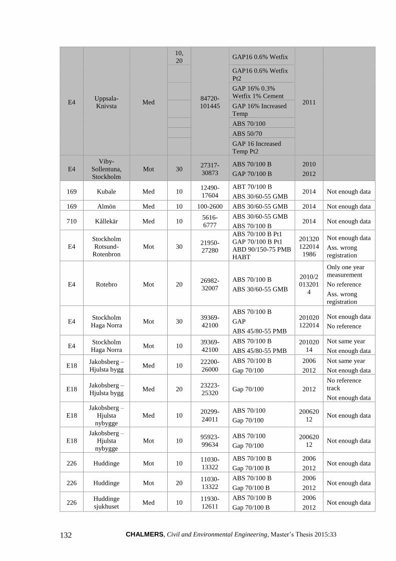
CHALMERS, Civil and Environmental Engineering, Master’s Thesis 2015:33 132
E4 Uppsala-
Knivsta Med
10,
20
84720-
101445
GAP16 0.6% Wetfix
2011
GAP16 0.6% Wetfix
Pt2
GAP 16% 0.3%
Wetfix 1% Cement
GAP 16% Increased
Temp
ABS 70/100
ABS 50/70
GAP 16 Increased
Temp Pt2
E4
Viby-
Sollentuna,
Stockholm
Mot 30 27317-
30873
ABS 70/100 B
GAP 70/100 B
2010
2012
169 Kubale Med 10 12490-
17604
ABT 70/100 B
ABS 30/60-55 GMB 2014 Not enough data
169 Almön Med 10 100-2600 ABS 30/60-55 GMB 2014 Not enough data
710 Kållekär Med 10 5616- 6777
ABS 30/60-55 GMB
ABS 70/100 B 2014 Not enough data
E4
Stockholm
Rotsund-
Rotenbron
Mot 30 21950-
27280
ABS 70/100 B Pt1
GAP 70/100 B Pt1
ABD 90/150-75 PMB
HABT
201320
122014
1986
Not enough data
Ass. wrong
registration
E4 Rotebro Mot 20 26982-
32007
ABS 70/100 B
ABS 30/60-55 GMB
2010/2
013201
4
Only one year
measurement
No reference
Ass. wrong
registration
E4 Stockholm
Haga Norra Mot 30
39369-
42100
ABS 70/100 B
GAP
ABS 45/80-55 PMB
201020
122014
Not enough data
No reference
E4 Stockholm
Haga Norra Mot 10
39369-
42100
ABS 70/100 B
ABS 45/80-55 PMB
201020
14
Not same year
Not enough data
E18 Jakobsberg –
Hjulsta bygg Med 10
22200-
26000
ABS 70/100 B
Gap 70/100
2006
2012
Not same year
Not enough data
E18 Jakobsberg –
Hjulsta bygg Med 20
23223-
25320 Gap 70/100 2012
No reference
track
Not enough data
E18
Jakobsberg –
Hjulsta
nybygge
Med 10 20299-
24011
ABS 70/100
Gap 70/100
200620
12 Not enough data
E18
Jakobsberg –
Hjulsta
nybygge
Mot 10 95923-
99634
ABS 70/100
Gap 70/100
200620
12 Not enough data
226 Huddinge Mot 10 11030-
13322
ABS 70/100 B
Gap 70/100 B
2006
2012 Not enough data
226 Huddinge Mot 20 11030-
13322
ABS 70/100 B
Gap 70/100 B
2006
2012 Not enough data
226 Huddinge
sjukhuset Med 10
11930-
12611
ABS 70/100 B
Gap 70/100 B
2006
2012 Not enough data

CHALMERS Civil and Environmental Engineering, Master’s Thesis 2015:33 133
226
Huddinge
sjukhuset
Med 20 11819-
12120
ABS 70/100 B
Gap 70/100 B
2004
2012 Not enough data
276 Åkersberga Med 10 6656-7700 ABS 70/100 B
Gap 70/100 B
2009
2012 Not enough data
276 Åkersberga Mot 10 45460-
46500
ABS 70/100 B
Gap 70/100 B
2009
2012
Not enough data
ABS data only
one year
E18 Örebro Med 20 71430-
84408
ABS 70/100 B
ABS 30/60-55-GMB 2013
No available
data
E20 Örebro Mot 20 0-23136 ABS 70/100 B
ABS 30/60-55 GMB 2013
Last
measurements
in 2012
6.20 Gothenburg,
Söderleden Mot
10,
20
1940-
10180
ABS 16 GMB
ABS 11 GMB
ABS PMB
2013/
2011 Date not clear
6.20 Gothenburg,
Söderleden Med 10
26432-
34688
ABS 16 GMB
ABS 11 GMB
ABS PMB
2013/
2011 Date not clear
169 Tjörn Med 10 13468-
17643 ABS 30/60-55 GMB 2014
Last
measurements
from 2013
E6/
E20 Sävenäsleden Med 10
15080-
20920
ABS GMB
ABS B
2003
2002
1980
Unreliable date
E4 Broänge-
Hökmark Med 10
156720-
164260
GAP16 100/150
ABS 16 100/150 2012
E12 Lycksele Med 10 151932-
158798
ABTS 11
ABTS 11 GMB 2012
E12 Lycksele Mot 10 307155-
309235
ABTS 11
ABTS 11 GMB 2012
E12 Storuman-
Stensele Med 10
245181-
252932
GAP 16
ABT 16 GMB
ABT 16 B 160/220
2011
E4 Gäddvik-
Nickbyn Med 10
72795-
89450
GAP 16
ABS 16 100/150 2012
E4 Gäddvik-
Nickbyn Mot 10
112038-
130608
ABS 16 GMB
ABS 16 100/150 2013
356 Boden Med 10 36079-
36989 GAP 50/80-55 GMB 2013 Not enough data