comparing phylogenetic and statistical classification methods for dna barcoding frederic austerlitz,...
TRANSCRIPT

Comparing phylogenetic and statistical classification methods
for DNA barcoding
Frederic Austerlitz, Olivier David, Brigitte Schaeffer, Sisi Ye, Michel
Veuille & Catherine Laredo

Testing the assignation methods
• Individual to be tested:– X1 : ATATGTACCTAGTA
– X2 : TTATCTACCTAGAA
• Reference sample :– 1_1: ATATGTACGTAGTA
– 1_2: ATATCTACGAAGTA
– 1_3: ATATCTACTAAGTA
– 2_1: ATATGTACGTAGTT
– 2_2: ATATGTACGAAGTT
– 2_3: ATTTCTACTAAGTT
Species 1
Species 2
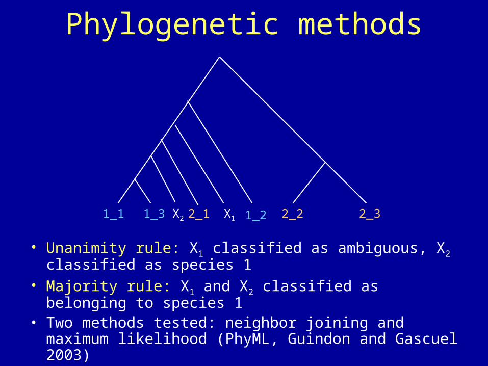
Phylogenetic methods
1_1 1_3 2_1 1_2 2_2 2_3X1
• Unanimity rule: X1 classified as ambiguous, X2 classified as species 1
• Majority rule: X1 and X2 classified as belonging to species 1
• Two methods tested: neighbor joining and maximum likelihood (PhyML, Guindon and Gascuel 2003)
X2

Node 0 Start with all the individualsto reach:
« individuals in each leave belong to the same species »
A: 5 B: 3 C: 8
CART (Classification And Regression Tree)
• Builds a classification tree from the reference sample
(Breiman et al., 1984, 1996)
Node 1
A: 5 B: 0 C: 4
Node 2
A: 0 B: 3 C: 4
Leave 1
A: 5 B: 0 C: 0
Leave 2
A: 0 B: 0 C: 4
Leave 3
A: 0 B: 0 C: 4
Leave 1
A: 0 B: 3 C: 0

node t = subset of individualsp (j | t) = relative proportion of individuals of class j in node t
JJ
1,...,
1 maximum
1,0,...,0,...,0,...,0,1 minimum for
Computing the impurity of the nodes
Impurity criterion at node t:
I(t) = - ∑j p(j|t) log p(j|t) entropy
I(t) = 1 - ∑j p(j|t)² Gini index
))(),...,(),...,1(()( tJptjptptI
PL + PR = 1
t
tLtR
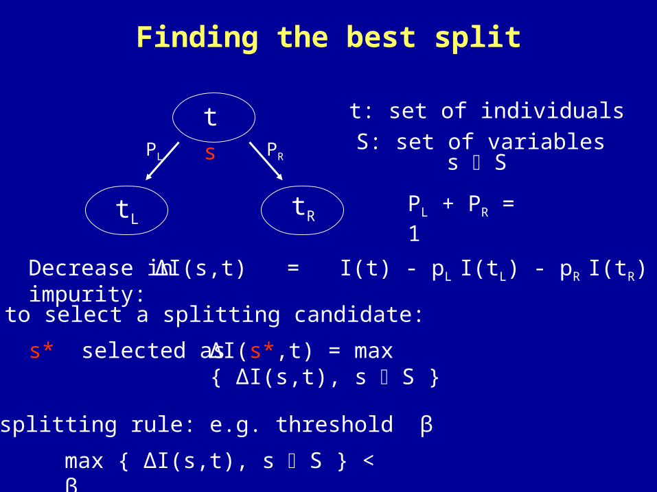
s PRPL s SS: set of variables
t: set of individuals
Finding the best split
ΔI(s*,t) = max { ΔI(s,t), s S }
ΔI(s,t) = I(t) - pL I(tL) - pR I(tR)
Rule to select a splitting candidate:
Decrease in impurity:
s* selected as
Stop splitting rule: e.g. threshold β
max { ΔI(s,t), s S } < β

Example:
I(t) = I(node0) = - ∑j p(j|t) log p(j|t)At node 0:
I(node0) = - [3/10 × log(3/10) + 3/10 × log(3/10) + 4/10 × log(4/10)]
3 species, 10 individuals, 4 variables
I(node0) = 1.0889
Species x1 x2 x3 x4 A a g c g A a g c g A a a a g B t t a g B t t a g B t a c g C a c a g C g c a g C a c a g C a c c g
Node 0A: 3/10, B: 3/10, C: 4/10

I(t) = - ∑j p(j|t) log p(j|t)
Splitting according to x1
Species x1 x2 x3 x4 A a g c g A a g c g A a a a g B t t a g B t t a g B t a c g C a c a g C g c a g C a c a g C a c c g
At node L: Ix1(nodeL) = - [0 + 3/3× log(3/3) + 0] = 0
Ix1(nodeR) = - [3/7× log(3/7) + 0 + 4/7× log(4/7)]At node R:
Ix1(nodeR) = 0.6829
A: 0, B: 3/3, C: 0 A: 3/7, B: 0, C: 4/7
Node 0A: 3/10, B: 3/10, C: 4/10
x1= t
Node L Node R
PR= 7/10PL= 3/10
ΔI(x1,t) = I(node0) - PL *Ix1(nodeL) - PR *Ix1(nodeR)
ΔI(x1,t) = 1.0889 - 0.3 × 0 - 0.7 × 0.6829 = 0.6109

I(t) = - ∑j p(j|t) log p(j|t)
At node L:
Ix2(nodeR) = - [0 + 0 + 4/4*log(4/4)] = 0
Species x1 x2 x3 x4 A a g c g A a g c g A a a a g B t t a g B t t a g B t a c g C a c a g C g c a g C a c a g C a c c g
Ix2(nodeL) = - [3/6*log(3/6) + 3/6*log(3/6) +0]
At node R:
Node 0A: 3/10, B: 3/10, C: 4/10
x2 = a,g,t
Node L Node RA: 3/6, B: 3/6, C: 0 A: 0, B: 0, C: 4/4
PR= 4/10PL= 6/10
ΔI(x2,t) = I(node0) - PL *Ix2(nodeL) - PR *Ix2(nodeR)
ΔI(x2,t) = 1.0889 - 0.6 *0.6931 - 0.4*0 = 0.6730
Ix2(nodeL) = 0.6931
Splitting according to x2

I(t) = - ∑j p(j|t) log p(j|t)
Ix3(nodeR) = - [2/4*log(2/4) + 1/4*log(1/4) + 1/4*log(1/4)] = 1.040
Species x1 x2 x3 x4 A a g c g A a g c g A a a a g B t t a g B t t a g B t a c g C a c a g C g c a g C a c a g C a c c g
At node L: Ix3(nodeL) = - [1/6*log(1/6) + 2/6*log(2/6) + 2/6*log(2/6)] = 1.031
At node R:
Node 0A: 3/10, B: 3/10, C: 4/10
x3 = a
Node L Node RA: 1/6, B: 2/6, C: 1/6 A: 2/4, B: 1/4, C: 1/4
PR= 4/10PL= 6/10
ΔI(x3,t) = I(node0) - PL *Ix2(nodeL) - PR *Ix2(nodeR)
ΔI(x3,t) = 1.0889 - 0.6 *1.031 - 0.4*1.040 = 0.0662
Splitting according to x3
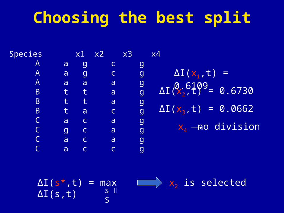
Species x1 x2 x3 x4 A a g c g A a g c g A a a a g B t t a g B t t a g B t a c g C a c a g C g c a g C a c a g C a c c g
ΔI(x2,t) = 0.6730
ΔI(s*,t) = max ΔI(s,t)s S
ΔI(x1,t) = 0.6109
ΔI(x3,t) = 0.0662
x4 no division
x2 is selected
Choosing the best split

Criterion: entropy
Software: RPackage: rpart
Implementation
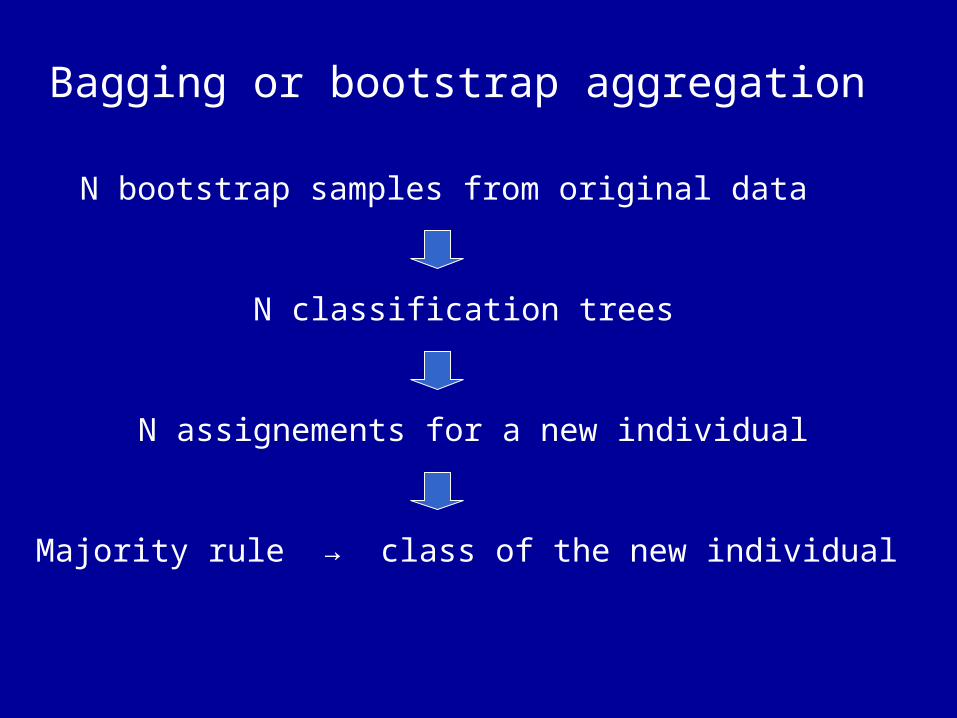
Bagging or bootstrap aggregation
N bootstrap samples from original data
N classification trees
N assignements for a new individual
Majority rule → class of the new individual

Simulation method
• one haploid population that splits into two (or more), T generations in the past.
• The ancestral population and the two new populations of constant size N.
• Sequences with mutation rate parameter of interest = 2N• Simulations performed with simcoal 2.1.2 (Excoffier et al)
T

Evaluation of the different classification methods
• We simulate n +1 individuals in each species.
• n individuals are considered as the reference samples, and the last one as the individual to test.
• Using repeated simulations, we compute the proportion of cases in which each test individual is correctly assigned to its species.
T

Parameters assumed for the simulation study
• = 3 (e.g. Litoria) or 30 (e.g. Astraptes)
• Reference sample size n = 3, 5, 10, 25
• Effective population size: N = 1000
• Separation time T = N/10, N/2, N, 5N or 10N
• Number of newly founded populations: from 2 to 5 In all cases, all populations assumed to be founded
simultaneously.

Comparison between phylogenetic methods
0.0%
20.0%
40.0%
60.0%
80.0%
100.0%
0 10 20 30
reference sample size
go
od
ass
ign
men
t ra
te
neighbor joining
PhyML
• 2 populations • Separation time = 500, = 3.

Effect of the number of populations
• = 3
0.00%
20.00%
40.00%
60.00%
80.00%
100.00%
2 3 4 5
Number of populations
go
od
ass
igm
ent
rate
phylo
cart
bagging
• = 30
0.00%
20.00%
40.00%
60.00%
80.00%
100.00%
2 3 4 5
Number of populations
go
od
ass
igm
ent
rate
phylo
cart
bagging
(Separation time: 500 generations, Reference sample size = 10)

Effect of the separation time
• = 3
• = 30
(4 populations, Reference sample size = 10)
0.00%
20.00%
40.00%
60.00%
80.00%
100.00%
100 1000 10000
Separation time
go
od
ass
igm
ent
rate
phylo
CART
Bagging
0.00%
20.00%
40.00%
60.00%
80.00%
100.00%
100 1000 10000
Separation time
go
od
ass
igm
ent
rate
phylo
CART
Bagging

Effect of the size of the reference sample
• = 3
• = 30
(4 populations, Separation time = 500)
0.00%
20.00%
40.00%
60.00%
80.00%
100.00%
0 5 10 15 20 25
Reference sample size
go
od
ass
igm
ent
rate
phylo
CART
Bagging
0.00%
20.00%
40.00%
60.00%
80.00%
100.00%
0 5 10 15 20 25
Reference sample size
go
od
ass
igm
ent
rate
phylo
CART
Bagging

Adding nuclear genes
• We considered the case where polymorphism of nuclear genes are also available.
• We assumed that– these genes were independent.– they all have the same (= 4N) value, equal
to the value for the cytoplasmic genes.– They do not show intragenic recombination or
they show it at a rate equal to the mutation rate (c = , i.e. 4Nc = ).

Adding nuclear genes
• Phylogenetic method• 2 populations• = 3, separation time = 500, reference sample size = 10
0%
20%
40%
60%
80%
100%
0 1 2 3 4 5
number of nuclear loci
go
od
ass
ign
men
t ra
te
without recombination no cyto
with recombination no cyto
without recombination + cyto
with recombination + cyto

Adding nuclear genes
• Phylogenetic method• = 30, separation time = 500, reference sample size = 10
0%
20%
40%
60%
80%
100%
0 1 2 3 4 5
number of nuclear loci
go
od
ass
ign
men
t ra
te
without recombination no cyto
with recombination no cyto
without recombination + cyto
with recombination + cyto

Application to real data
• Litoria (Schneider et al, 1998, Mol. Ecol. 7, 487–498).
– 4 species– Average sample size: 43.75– average = 1.54
92%
93%
94%
95%
96%
97%
98%
99%
100%
0 2 4 6 8 10 12
reference sample size
go
od
ass
ign
men
t ra
te
phylo
CART

Application to real data
• Astraptes (Hebert et al 2004. Proc. Natl Acad. Sci. USA 101,14812–14817)
– 12 species– Average sample size: 38.8– average = 23.5
90%
91%
92%
93%
94%
95%
96%
97%
98%
99%
100%
3 4 5 6 7 8 9 10
Reference Sample size
Go
od
ass
ign
men
t ra
te
phylo
CART

Application to real data• Cowries (Meyer et al (2005) PLoS Biol 3: e422)
– 357 taxa (species/subspecies)– Average sample size: 5.7– average = 2.93
90%91%92%
93%94%95%96%97%98%
99%100%101%
0 5 10 15 20 25 30
reference sample size
go
od
ass
ign
men
t ra
te
phylo
CART

Conclusions• Regarding phylogenetic methods, the maximum
likelihood method performs better than the neighbor joining.
• CART performs better than phylogenetic methods for poorly informative data (low value)
• but not for more polymorphic data (high value)
• Adding nuclear loci can help, but at a quite high cost.
• Recombination improves the phylogenetic method for low values (Ongoing work for CART).

Perspectives
• Developing a statistical method to put a confidence level on a given assignation.
• Evaluating other classification methods (learning methods)