comparing models for growth and management of forest tracts

2 9 Comparing Models for Growth and Management of Forest Tracts

J.J. Colbert,' Michael Schuckers2 and Desta Fekedu legn2

Abstract

The Stand Damage Model (SDM) is a PC-based model that is easily installed, calibrated and ini- tialized for use in exploring the future growth and management of forest stands or small wood lots. We compare the basic individual tree growth model incorporated in this model with alternative models that predict the basal area growth of trees. The SDM is a gap-type simulator. It is a non-spatial, individual sample-tree diameter growth model, following the work of Botkin, Shugart and others. Within SDM, the basic growth model is adjusted to account for shading, competition and climate. Here we make those adjustments by calibrating the growth model to historical data for individual sample trees. We fit alternative sigmoid growth models to the same historical data and compare these models' ability to predict short-term (5-year) and longer term growth of trees. Accuracy and potential effects of bias are discussed relative to the age and source locations of sample trees used in this study.

Introduction

The Stand Damage Model (SDM), a component of the Gypsy Moth Life System Model, calculates tree diameter growth, current diameter and height, and tree mortality for each year of a simulation. The model is a distance-independent, tree-growth simulator, a gap model based on the work of Botkin (1993), Shugart (1984) and others. Each year, the model calculates the diameter growth of trees as a function of relative stocking (a measure of tree crowding), shading, heat and defoliation. The model can be used to predict future growth of a forest stand or tract that the user wants to con- sider as a homogeneous unit. The user can design tree removals to simulate various kinds of silvicultural regimes at any year of a simulation. The user provides data for management actions, including the year of entry, selection criteria for removals and species-specific targets. The model has the ability to simulate predefined defoliation scenarios over a 20-year period from the initial stand conditions or the user can decide to have defoliation occur at any time and at intensities as input through the

USDA Forest Service, USA Correspondence to: [email protected]

Department of Statistics, West Virginia University, USA

0 CAB International 2003. Modelling Forest Systems (eds A. Amaro, D. Reed and P. Soares)

336 /.I. Colbert et al.

user interface. With the predefined scenarios come a large number of graphs and tables automatically generated to assist the user in assessing possible future impacts of gypsy moth defoliation.

Weather drives photosynthesis and tree growth. Within the model, a cumula- tive heat unit measure, degree-days above a single threshold (4.4"C), is used for all tree species as a primary driver of diameter growth. Default constant weather data can be overridden by entering weather variation for each year simulated. Tree mortality comprises three factors: a base rate, stress-induced mortality and gypsy moth defoliation-induced mortality. The base rate is increased as diameter growth is reduced. Following mortality calculations, tree growth is updated for the residual stems, and new stems are recruited to the smallest classes.

For details on model formulation or computational algorithms, see Colbert and Sheehan (1995). Colbert and Racin (1995,2001) provide users with directions for use of the model, and Racin and Colbert (1995) give a complete description of the program structure for the user interface system. The model interface now includes parameters for 71 tree species or species groups. The user can add up to 10 additional species for a stand simulation; 20 species can be included in a single simulation. Seven additional categories for including non-commercial or other unidentified species (grouped by susceptibility to defoliation as conifers or deciduous trees) allow users to provide a more complete and accurate set of initial conditions. In addition to tree counts by species and diameter class, you can assign one of three soil-moisture categories for the stand. Users supply information on defoliation history (in broad categories by species for the 2 years prior to the simulation) and describe defoliation scenarios for each species each year as a percentage for the overstorey and for the understorey.

State of the Art

As a stand-alone model, the SDM provides the user with the ability to assess the effects of defoliation on a tree and stand level. Through multiple simulations, the model can be used to assess the possible future impacts of a gypsy moth outbreak on a large forested area (Colbert et al., 1997). The model has also been used for a much broader assessment of possible forest impacts of the gypsy moth (Gottschalk et al., forthcoming; Guldin et al., forthcoming). The model can also be used as a stand growth and forest management simulator, disregarding the gypsy moth and associated impacts. Through the user interface, one can describe a forest stand, set growth parameters, design future management entries, and project an initial inven- tory into the future to assist in viewing the effects of various scenarios. The current model can carry a stand through cutting cycles, but the current regeneration algorithms are limited and research is under way to enhance the models for predicting regeneration success and growth of young stands.

General Technical Report NE-211 (Liebhold et al., 1995) was the source for species feeding preference of the gypsy moth; data from Botkin (1993) and Shugart (1984) contributed significantly to the formulations used in the model. To better understand and interpret the current SDM, review the documentation for Version 1.0 (Colbert and Racin, 1995; Colbert and Sheehan, 1995; Racin and Colbert, 1995). The 'HOW-TO' document (Colbert and Racin, 2001) provides an installation diskette and a complete description of the updates and enhancements for Version 2.0 of the model and a tutorial for use of the new data entry system. Plot data from any design of fixed area and prism point samples are converted automatically into both stand- level summary tables and an initial-conditions file for further use in simulations.

Comparing Models for Growth and Management 337

The user interface allows data to be stored and retrieved through the expanded and enhanced menu system. Documentation and software downloads can be found at the US Forest Service website: www.fs.fed.us/ne/morgantown/4557/gypsymth. Available at this website are descriptions of the models and related publications as well as links for downloading this and other models that have been developed.

Included with the 'How-To' document is a PC/Windows installation diskette. Once installed, the user is provided with two example data sets. One is from a series of variable-radius plots from a stand in Ohio. The second is from a fixed area three- plot cluster in Pennsylvania. These example data are used in the tutorial section for learning plot data entry. In addition, there is an Excel file that contains a complete 15-year history of the three-plot cluster for use as a validation and test data set.

Platforms supported by the Stand Damage Model

The model currently runs under MS-DOS and within a DOS window or emulator under Windows 3.1/95/98/NT on Intel or compatible processor^.^ It operates as a DOS package of programs, using a graphical interface for management of input and output data, controlling simulations and viewing results. The model can run on older computers and does not require more than the base 640K of memory, although usage is enhanced by a mouse for easy access and movement within and among windows within the user interface. Instructions are included with the installation package for running the program from Windows 3.1 with the included PIF and icon files or from Windows 95/98/NT.

Related resources

It is possible to completely re-parameterize the model for locations outside North America. The data required for adding species to the model can be found in basic dendrology texts. In North America we used the Textbook of Dendrology (Harlow et al., 1979), the Silvics of North America volumes compiled by Burns and Honkala (1990a, b), and Trees of the Southeastern United States (Duncan and Duncan, 1988) as sources to generate parameters. For scientific and common names, we followed the nomenclature in Checklist of United States Trees (Little, 1979). Oaks of North America (Miller and Lamb, 1985) was a valuable resource for searches within specific families or genera. Knowing Your Trees (Collingwood and Brush, 1978) was used to assess tree-crown shape in assigning stocking classes, and Important Forest Trees of the Eastern United States (USDA Forest Service, 1991) was the source of information for each species. The 'How-To' publication (Colbert and Racin, 2001) provides a complete guide to building parameter files for the model.

Methodology

Forest conditions in the mid-Atlantic region of the USA are quite variable, with con- tinental climate and annual rainfall from 50 to 180+ cm (generally in the range of

The use of trade, firm or corporation names is for the information and convenience of the reader. Such use does not constitute an official endorsement or approval by the US Department of Agriculture or Forest Service of any product or service to the exclusion of others that may be suitable.

338 I.]. Colbert et al .

100-130 cm) in the areas where managed forests are most prevalent. Rainfall is generally well distributed throughout the year. The forests we studied are considered to be mixed mesophytic and consisted of oak-dominated, mixed oak-hickory, or oak-maple forest types. These forest stands are usually quite diverse in canopy com- position and contain from five to 20 or more different tree species. Elevations range from the coastal plains of Delaware, just 2-10 m above sea level, to the forests of the more interior central Pennsylvania and West Virginia mountains, which range from 350 to 900 m above sea level. Here, our study sites range from 400 to 600 m elevation. In Ohio, stands were located on the Dorr Run management unit of the Athens district of the Wayne National Forest, which is 210-320 m elevation.

Analyses of four forest tree basal-area growth models were carried out using data from the states of Delaware (DE), Pennsylvania (PA), West Virginia (WV) and Ohio (OH) in the mid-Atlantic region of the USA. We fitted these with non-linear sigmoid growth models which are described in detail by Fekedulegn et al. (1999). The four-parameter models we chose to utilize in this study have been shown to be adequate for modelling sigmoid growth with sufficient flexibility and good statistical properties (Draper and Smith, 1981; Schnute, 1981; Myers, 1986; Vanclay, 1994). These models were fit to basal-area data derived from radial increment data and estimates of inner radius and age.

Source data

A total of 190 radial growth-increment samples were used. The data were obtained from southern red oak (Quercus falcata) and white oak (Quercus alba) from the coastal plain in central and southern DE; northern red oak (Quercus rubra) from the ridge- and-valley area of central PA; northern red oak on the Coopers Rock State Forest in north central WV; and northern red oak from OH. Table 29.1 provides the numbers of sample data and type. All samples were taken at breast height (137 cm). Increment cores were taken with 4.3 mm borers, and disc samples were taken from felled trees. All increment core samples were taken aiming through the tree centre, attempting to get as close to the pith as possible.

Increment cores were first dried and glued in place with water-soluble glue on top of wood mounts of approximately 18 mm high x 8 mm wide cross-section. The mount top is bevelled so that it contains a groove 4 mm across that runs the length of the mount. Samples were oriented vertically and sanded using fine (400-1200) grit to expose cell structure. Annual radial increments were measured to the nearest 0.001 mm on a measuring stage and the radius and age at the inner edge of the innermost ring were estimated using a 1-mm scaled circular ruler, taking into con- sideration the curvature of the earliest growth rings and the width of those same rings. In some instances, on increment core samples and on all disc samples we were

Table 29.1. Sample counts by location, type and tree species.

Location TY pe Species Number

Delaware (DE) I Ca Quercus falca ta 24 I C Quercus alba 32

Pennsylvania (PA) IC Quercus rubra 26 West Virgina (WV) Disc Quercus rubra 21 West Virginia (WV) IC Quercus rubra 60 Ohio (OH) I C Quercus rubra 28

alC = increment core sample.


able to provide data from the pith at age 0. Basal area (inside bark) series were then produced, assuming circular cross-sections at breast height.

Sigmoid models

The non-linear models fitted were the following:

(1) Richards

(2) Weibull

(3) Chapman-Richards

(4) von Bertalanffy

proposed by (1) Richards (1959), (2) Ratkowsky (1983), (3) Turnbull (1963), Pienaar and Turnbull (1973) and (4) von Bertalanffy (1957). It should be noted that all parameters are assumed to be positive (&, &, P2, P3 > 0) for all models; in Equation 2, PI < Po; in Equation 3, PI < 1; and in both Equations 3 and 4, P3 < 1. For the tree species used, growing in North America, biological bounds were constructed. Maximum basal area for the red oaks is less than 2 m2 and less than 5 m2 for Q. alba. We set the upper bound for & to be 8 m2 and the lower bound to be 0.1 m2 for all runs of each model. We used the NLIN procedure (SAS, 2000) with the Marquardt (1963) method to estimate the parameters for each model and basal-area series, supplying the par- tial derivatives (Fekedulegn et al., 1999). We found convergence to be quite sensitive to the starting values used. We first used modal initial conditions, estimated from the data as described in Fekedulegn et al. (1999). Then we used the distribution of values resulting from the first application of the NLIN procedure to create a new initial search grid (Table 29.2) used for the final runs of the NLIN procedure.

To assess the predictive power of each model, we truncated each data set and refitted the models to each truncated data set. This allowed us to examine differences and produce tests of each model's ability to predict future basal area.

Table 29.2. Initial search grid (L, lower bound; U, upper bound; S, step size).

Model

Richards (R) L U S

Weibull (W) L U S

Chapman-Richards (C-R) L u S

von Bertalanffy (VB) L U S

340 1.1. Colbert et at.

Statistical summaries are provided for parameters for each model. We tested the differences among the models' ability to fit the data by examining the number of samples where the convergence criteria were met. Because the fit residuals are not normally distributed, we used a non-parametric test procedure to test for location and scale differences across a one-way classification (Wilcoxon). We calculated the mean square error (MSE) for each fit and tested difference among the models. We explored parameter interactions and consistency of fits among sites and among species. We also examined the interactions among parameters within models and the values of fi,, among models since this parameter is the asymptotic basal area as the tree reaches maturity.

Results

To judge the quality of models and fitting procedures, we looked at the number of samples where the convergence criteria were met. Of the 380 total series, the Chapman-Richards model consistently converged most often, followed by the Richards, Weibull and finally the von Bertalanffy model (Table 29.3).

For all models, the fitting procedure converged for the majority of these data and there was no significant difference among the numbers of series fitted for each model. It can also be seen that the length of the data series did not have a consistent effect on convergence. There was no data set that was significantly different in the number of series converging (Table 29.4).

Among data sets, the Chapman-Richards model consistently converged most often. It should be noted that we first attempted to use less dense initial grids and found that the procedure did not converge for a very large number of samples, across all models.

We examined MSE for each model, series length and source data set and found that there was no significant difference among these classifications. We found the choice of limits and mesh size to have a large effect on the number of converging series and the quality of the fit (MSE). We found good quality fits (MSE < lop4) in 87.5% of the non-converging samples. It should be noted that since the procedure used did not permit the inclusion of non-constant constraints (boundary conditions) among parameters, there was some data truncation for early growth for some samples when fitting the von Bertalanffy model. It is sufficient that P O 1 P 3 > 4 for i) to be positive for all t. When this condition is not met, i) will remain undefined for small t, and the associated data are ignored during the fitting procedure.

Table 29.3. Adequacy of Marquardt fit to full and reduced series (counts in parentheses).

Full Reduced Total

Model YO

Richards (R) 83 (1 58)

Weibull (W) 71 (1 35)

Chapman-Richards (C-R) 96 (1 82)

von Bertalanffy (VB) 63 (1 20)


Table 29.4. Percentages of Marquardt fit among data sets and models.

Model

Richards (R) 61 85 73 82 74 85 Weibull (W) 87 29 81 85 76 57 Chapman-Richards (C-R) 97 98 88 95 88 100 von Bertalanffy (VB) 62 81 62 64 45 85

Sites: Q.a. - DE, Q. alba; Q.f. - DE, Q. falcata; IC -West Virginia increment core samples; D - West Virginia disc samples.

Model fits: graphs and residual plots

While improvement can be made in obtaining convergence, results obtained on samples that did not converge often appear to be adequate and represent the data well throughout the range of those data. The errors about the non-converged fitted curves are often no worse or even better than another sample taken at another radius from the same tree where convergence criteria were met. The ability to find an adequate fit does not appear to be associated with either the length or starting point of the data series. Figure 29.1 shows the fitted summaries for such a sample. The truncated series did not converge. Convergence was obtained for both series from a second increment core sample taken from the same tree. It was found that problems with convergence did not appear to be associated consistently with either the full or truncated series. Influences such as individual tree release, weather or insect defoliation can cause fluctuations in the growth pattern that are not well represented by these models.

Predictions

We examined 5-, 10- and 15-year predictions. Figure 29.2 shows two trees where the truncated series demonstrates that a prediction from the truncated model can be used for predicting the trend of diameter growth. Table 29.5 shows the values for each of the predictions, along with actual data.

Table 29.5. Actual and predicted basal area for two trees; Y, measured basal area; p, predicted basal area, full data series; t, predicted basal area, truncated data series.

PIa 0 5 10 15

aPrediction interval length in years.

342 1.). Colbert et al.

Model asymptotes (theoretical maximum values)

We examined the parameters for each model. Po was the only parameter that was comparable among models. We f o u n d that the truncated series ( P = 0.0104) a n d the

-0.001 1 6 11 1621 2631 3641 4651 566166

Age (years)

Age (years)

Age (years) -0.001 -

I 6 11 I6 21 26 31 36 41 46 51 56 61 66 Age (years)

Fig. 29.1. Basal area data and Chapman-Richards model, with 95% confidence intervals: (a) converged to the full data set; (b) residuals about Yfrom (a); (c) non-convergence to the truncated data set; (d) residuals for (c). Note that the residuals are clustered closer to the curve in the truncated fit.

-0.05 4 10 16 22 2834404652 58 6470 76

Age (years)

4.10 0 3 9 15 21 27 33 39 45 51 57 63 69

Age (years)

Fig. 29.2. The data, fitted Chapman-Richards model, and 95% confidence intervals (a) using the first 59 years of a Pennsylvania sample and (b) using the first 64 years of an Ohio sample (seeTable 29.5).


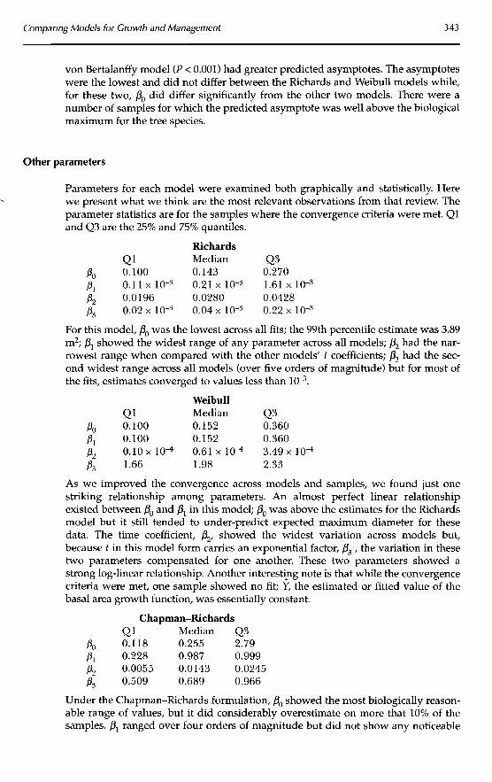
von Bertalanffy model (P < 0.001) had greater predicted asymptotes. The asymptotes were the lowest and did not differ between the Richards and Weibull models while, for these two, Po did differ significantly from the other two models. There were a number of samples for which the predicted asymptote was well above the biological maximum for the tree species.

Other parameters

Parameters for each model were examined both graphically and statistically. Here -, we present what we think are the most relevant observations from that review. The

parameter statistics are for the samples where the convergence criteria were met. Q1 and Q3 are the 25% and 75% quantiles.

Richards Q1 Median Q3

Po 0.100 0.143 0.270 p, 0 . 1 1 ~ 1 0 - ~ 0.21~10-3 i .6 ix io-3 p, 0.0196 0.0280 0.0428 p,, 0.02~10-3 o . o ~ x ~ o - ~ 0.22~10-3

For this model, Po was the lowest across all fits; the 99th percentile estimate was 3.89 m2; 4 showed the widest range of any parameter across all models; & had the nar- rowest range when compared with the other models' t coefficients; P3 had the second widest range across all models (over five orders of magnitude) but for most of the fits, estimates converged to values less than 10".

Weibull Q1 Median Q3

Po 0.100 0.152 0.360 Dl 0.100 0.152 0.360 p, 0 . 1 0 ~ 10-4 0.61 lo4 3 . 4 9 ~ 10-4 p3 1.66 1.98 2.33

As we improved the convergence across models and samples, we found just one striking relationship among parameters. An almost perfect linear relationship existed between Po and PI in this model; Po was above the estimates for the Richards model but it still tended to under-predict expected maximum diameter for these data. The time coefficient, P2, showed the widest variation across models but, because t in this model form carries an exponential factor, P3, the variation in these two parameters compensated for one another. These two parameters showed a strong log-linear relationship. Another interesting note is that while the convergence criteria were met, one sample showed no fit; Y, the estimated or fitted value of the basal area growth function, was essentially constant.

Chapman-Richards Ql Median Q3

Po 0.118 0.255 2.79 p, 0.228 0.987 0.999 p2 0.0055 0.0143 0.0245 p3 0.509 0.689 0.966

Under the Chapman-Richards formulation, Po showed the most biologically reasonable range of values, but it did considerably overestimate on more that 10% of the samples. PI ranged over four orders of magnitude but did not show any noticeable

344 1.1. Colbert et al.

interaction with other parameters. Except for the Weibull form, P3 showed the nar- rowest range of variability, with the exception of one sample.

No consistent pattern emerged among species or among sites in the parame- terization of these models except that P3 in the Weibull model shows some slight location dependence. These differences are mitigated by the fact that the range in differences are similar to what is obtained within West Virginia data between those samples taken from whole-tree dissections and those taken from increment cores.

Discussion and Conclusions

Each of these models will provide reasonable fit to radial increment data and permit estimates of future basal area under nominal conditions. There is consistency between models in terms of MSE. Research to date suggests that MSE is a better screening criterion than meeting SASS PRK NLIN convergence criteria. We attempted to use other fitting methods but found that the Marquardt method performed best. To strengthen our understanding of the power and consistency of these models to perform across this region, we plan to expand the data to include balance among species and to classify our analyses to account for canopy strata and site factor effects within species. We will fit data from older trees to ascertain how tree age affects parameters, particularly the asymptote. We will explore the ranges for parameters of these models that give rise to realistic trends for mature and over-mature trees. As mentioned earlier, convergence is highly dependent on starting values. We found that the use of a starting grid will usually provide good results. When boundary conditions are considered, convergence and the quality of final values can be further ensured. Some care must be taken to deal with non-linear boundary conditions, which may not be used under some procedures. We plan to compare these models with growth models used in forest management in this region and with the diameter growth model used as the basis for predicting diameter increment in forest gap simulators.

References

Botkin, D.B. (1993) Forest Dynamics: an Ecological Model. Oxford University Press, New York, 309 pp.

Burns, R.M. and Honkala, B.H. (technical coordinators) (1990a) Silvics of North America. 1. Conifers. Agriculture Handbook 654. US Department of Agriculture, Washington, DC, 675

PP . Burns, R.M. and Honkala, B.H. (technical coordinators) (1990b) Silvics of North America. 2.

Hardwoods. Agriculture Handbook 654. US Department of Agriculture, Washington, DC, 877 pp.

Colbert, J.J. and Racin, G. (1995) User's Guide to the Stand-Damage Model: a Component of the Gypsy Moth Life System Model (Version 1.1). General Technical Report NE-207. US Department of Agriculture, Forest Service, Northeastern Forest Experiment Station, Radnor, Pennsylvania, 38 pp. 11 computer disk (3$ in.)].

Colbert, J.J. and Racin, G. (2001) How to Use the Stand-Damage Model, Version 2.0. General Technical Report NE-281. US Department of Agriculture, Forest Service, Northeastern Forest Experiment Station, Newtown, Pennsylvania, 79 pp. [I computer disk (3; in.)].

Colbert, J.J. and Sheehan, K.A. (1995) Description of the Stand-Damage Model: Part of the Gypsy Moth Life System Model. General Technical Report NE-208. US Department of Agriculture, Forest Service, Northeastern Forest Experiment Station, Radnor, Pennsylvania, 111 pp.


Colbert, J.J., Perry, P. and Onken, B. (1997) Preparing for the gypsy moth: design and analysis of stand management. Dorr Run, Wayne National Forest. In: Communicating the Role of Silviculture in Managing the National Forests: Proceedings of the National Silviculture Workshop. 19-22 May, Warren, Pennsylvania General Technical Report NE-238. US Department of Agriculture, Forest Service, Northeastern Forest Experiment Station, Radnor, Pennsylvania, pp. 76-84.

Collingwood, G.H. and Brush, W.D. (1978) Knowing Your Trees. American Forestry Association, Washington, DC, 389 pp.

Draper, N.R. and Smith, H. (1981) Applied Regression Analysis, 2nd edn. John Wiley & Sons, New York, 709 pp.

Duncan, W.H. and Duncan, M.B. (1988) Trees of the Southeastern United States. University of Georgia Press, Athens, Georgia, 322 pp.

Fekedulegn, D., Mac Siurtain, M.P. and Colbert, J.J. (1999) Parameter estimation of nonlinear growth models in forestry. Silva Fennica 33,327-336.

Gottschalk, K.W., Colbert, J.J. and Guldin, J.M. (forthcoming). Modeling gypsy moth-related tree mortality under different outbreak and management scenarios in Ozark-Ouachita Interior Highlands forests. In: Proceedings, Upland Oak Ecology, A Symposium on History, Current Conditions, and Sustainability: 8-10 October 2002, Fayetteville, Arkansas. US Department of Agriculture, Forest Service, Southern Research Station, Asheville, North Carolina, GTR-SRS-xx.

Guldin, J.M., Thompson, F.R., Richards, L.L. and Harper, K.C. (forthcoming) Status and trends in vegetation. In: Ozark-Ouachita Highlands Assessment: Terrestrial Vegetation and Wildlife. US Department of Agriculture, Forest Service, Southern Research Station, Asheville, North Carolina.

Harlow, W.M., Harrar, E.S. and White, F.M. (1979) Textbook of Dendrology: Covering the Important Forest Trees of the United States and Canada, 6th edn. McGraw-Hill, New York, 510 pp.

Liebhold, A.M., Gottschalk, K.W., Muzkia, R.-M., Montgomery, M.E., Young, R., O'Day, K. and Kelley, B. (1995) Suitability of North American Tree Species to Gypsy Moth: a Summary of Field and Laboratory Tests. General Technical Report NE-211. US Department of Agriculture, Forest Service, Northeastern Research Station, Radnor, Pennsylvania, 34 pp.

Little, E.L. Jr (1979) Checklist of United States Trees (Native and Naturalized). Agriculture Handbook 541. US Department of Agriculture, Washington, DC, 375 pp.

Marquardt, D.W. (1963) An algorithm for least squares estimation of nonlinear parameters. Journal of the Society of Industrial and Applied Mathematics 11,431-441.

Miller, H. and Lamb, S. (1985) Oaks of North America. Naturegraph Publishers, Happy Camp, California, 327 pp.

Myers, R.H. (1986) Classical and Modern Regression with Applications. Duxbury Press, Boston, Massachusetts, 359 pp.

Pienaar, L.V. and Turnbull, K.J. (1973) The Chapman-Richards generalization of von Bertalanffy's growth model for basal area growth and yield in even-aged stands. Forest Science 19(1), 2-22.

Racin, G. and Colbert, J.J. (1995) Guide to the Stand-Damage Model Interface Management System. General Technical Report NE-209. US Department of Agriculture, Forest Service, Northeastern Research Station, Radnor, Pennsylvania, 149 pp.

Ratkowsky, D.A. (1983) Nonlinear Regression Modelling. Marcel Dekker, New York, 276 pp. Richards, F.J. (1959) A flexible growth function for empirical use. Journal of Experimental Botany

10,290-300. SAS (2000) SAS Online Doc Version 8, February 2000, SAS Institute, Cary, North Carolina. Schnute, J. (1981) A versatile growth model with statistically stable parameters. Canadian

Journal of Fisheries and Aquatic Sciences 38,1128-1140. Shugart, H.H. (1984) A Theory of Forest Dynamics: the Ecological Implications of Forest Succession

Models. Springer-Verlag, New York, 278 pp. Turnbull, K.J. (1963) Population dynamics in mixed forest stands: a system of mathematical

models of mixed growth and structure. PhD dissertation, University of Washington. United States Department of Agriculture, Forest Service (1991) Important Forest Trees of the

Eastern United States. FS-466. US Department of Agriculture, Forest Service, Washington, DC, 111 pp.

346 I.]. Colbert et al.

Vanclay, J.K. (1994) Modelling Forest Growth and Yield. CAB International, Wallingford, UK, pp. 380.

von Bertalanffy, L. (1957) Quantitative laws in metabolism and growth. Quarterly Review of Biology 32,218-231.

comparing models for growth and management of forest tracts

Documents