comparing living costs in australian capital cities · 2008-09-09 · comparing living costs in...

32nd CONFERENCE OF ECONOMISTS

29th September - 1st October 2003

AUSTRALIAN NATIONAL UNIVERSITY

Comparing Living Costs in Australian Capital CitiesA Progress Report on Developing Experimental Spatial Price Indexes

for Australia

Alex Waschka, William Milne, Jonathon KhooTim Quirey and Shiji ZhaoAnalytical Services Branch

Methodology DivisionAustralian Bureau of Statistics

The views expressed in this paper are the authors' and do not necessarily reflect those of the Australian Bureau of Statistics. Where quoted or used, they should be attributed to the authors.

Acknowledgments

This research has been undertaken with enormous support and assistance from both the Analytical Services Branch and the Prices Branch of the Australian Bureau of Statistics. We would like to especially thank Paul McCarthy, Ken Tallis, Keith Woolford and Michael Anderson for their continued guidance and patient advice. We are also very grateful to the staff of the Consumer Price Index Section for their help. In particular, we would like to thank Terry Offner, Margaret Dinan, Lauren Moran, Nadia Dugec, Dana Olejniczak and Sarah Dexter. Of course, we are responsible for any errors or omissions.


for Australia

Contents

Abbreviations

Executive Summary

1. Introduction

2. EKS Index Formula

3. Data Treatment and Index Construction

3.1 Data Structure3.2 Data Treatment Methods3.3 Missing Groups

4. Results

4.1 Spatial Price Indexes4.2 A Brief Analysis4.3 Per Capita Consumption Volumes by CPI Group

5. Summary and Future Research

Endnotes

Bibliography

Appendix 1: EKS Spatial Price Index Formula

Appendix 2: Statistical Properties of a Multilateral Index

Appendix 3: Index Construction Method

Appendix 4: Nominal and Real Per Capita Expenditures

Appendix 5: Household Characteristics of the Eight Capital Cities, 1998 - 99

Appendix 6: The Classification of CPI Data

AbbreviationsABS: Australian Bureau of Statistics

CPI: Consumer Price Index

EA: Elementary Aggregate

EC: Expenditure Class

EKS: Elteto, Koves and Szulc

HES: Household Expenditure Survey

HECS: Higher Education Contribution Scheme

GP: General Practitioner

OECD: Organisation for Economic Cooperation and Development

PPP: Purchasing Power Parities

TAFE: Technical and Further Education

Executive SummaryThe Australian Bureau of Statistics (ABS) has for many years published the Consumer Price Index (Consumer Price Index, Australia cat. no. 6401.0). The Consumer Price Index (CPI) measures the movements in retail prices of goods and services commonly purchased by metropolitan households. Although a separate index is available for each of the 8 capital cities (i.e. Sydney, Melbourne, Brisbane, Adelaide, Perth, Hobart, Darwin and Canberra), the eight indexes cannot be used to compare price levels between the cities.

This project assesses the feasibility of using existing price data collected for the CPI to produce experimental measures of price differences between the eight capital cities (i.e. spatial price indexes). The indexes cover the year ended June 2002 and were calculated using a multilateral EKS formula. This paper seeks comments on our work so far and suggestions for improving the indexes.

Most price observations in the CPI dataset appeared to be suitable for spatial comparisons. However, prices observations for some "services", such as "housing" and "miscellaneous" were found to be unsuitable and have not been included in the spatial indexes for the time being.

Our preliminary assessment suggests that the spatial price indexes look broadly plausible. However, for some "services", the index numbers show wider gaps than expected, which we are still unable to fully explain at the moment.

This paper is a report of our work-in-progress. We admit that the indexes are imperfect (particularly for certain services - such as health, transportation and education). We want to improve the indexes in the future and would be grateful for readers' comments and suggestions for improvements. In the meantime, they should NOT be used for policy or for other purposes until the ABS validates the statistics and publishes them in an official publication.

For further information about this project, contact Alex Waschka on 02 6252 6992 or email [email protected] , or Shiji Zhao on 02 6252 6053 or email [email protected].


for Australia

1. Introduction

The Australian Bureau of Statistics (ABS) has for many years published the Consumer Price Index (Consumer Price Index, Australia cat. no. 6401.0). The Consumer Price Index (CPI) measures the movements in retail prices of goods and services commonly purchased by metropolitan households. Although a separate index is available for each of the 8 capital cities (i.e. Sydney, Melbourne, Brisbane, Adelaide, Perth, Hobart, Darwin and Canberra), the eight indexes cannot be used to compare price levels between the cities.

This project assesses the feasibility of using existing price data collected for the CPI to produce experimental measures of price differences between the eight capital cities (i.e. spatial price indexes). The indexes cover the year ended June 2002 and were calculated using a multilateral EKS formula.

Most price observations in the CPI dataset appeared to be suitable for spatial comparisons. However, prices observations for some "services" (i.e. "housing" and "miscellaneous") were found to be unsuitable and have not been included in the indexes at this stage.

The paper is structured as follows. Section 2 introduces the price index formula used in this study. Section 3 describes the data sources and how we transformed the data into a form that is suitable for spatial comparisons. The results are presented in Section 4, whilst Section 5 summarises the study.

2. EKS Index Formula

This study uses the multilateral EKS formula to construct spatial price indexes (See Appendix 1 for the details of the formula). This formula has been used by the OECD's International Comparison Program (OECD, 1993) in the construction of official PPPs.

We decided to use the EKS index formula for two reasons:

It can be used to derive and compare real consumption statistics between cities (see the factor 1.reversal test in Appendix 2); and

It does not require prices of specific commodities to be available in every city. Rather, price 2.comparisons can be made as long as prices are available in at least two cities. The use of the EKS index, therefore, allowed us to maximise use of available information.

The EKS index has several useful statistical properties (as described in Appendix 2). However, as the EKS index does not pass the "consistency in aggregation" test, readers should not attempt to derive higher-level indexes by aggregating its component indexes.

3. Data Treatment and Index Construction

In this study, spatial price indexes were constructed based on the data which the ABS uses in compiling the quarterly CPI time series. The price samples in the CPI dataset were collected from the eight cities. They are similar in their broad coverage of consumption goods and services but differ in product specifications between cities to take account of local conditions.

A major task of this project was converting this CPI dataset into a form suitable for spatial indexes. This was not a straightforward exercise as the CPI dataset is extremely large and the conversion involved a large amount of complex data adjustment and treatment methods. In this paper we present a brief overview of the methods used to transform the CPI dataset into a spatially comparable dataset.

3.1 Data Structure

The CPI, as a measure of price inflation for the household sector, covers an extensive range of goods and services available for purchase by metropolitan households. It consists of 11 groups, namely:

Food;1.Alcohol and tobacco;2.Clothing and footwear;3.Housing;4.Household furnishings, supplies and services;5.Health;6.Transportation;7.Communication;8.Recreation;9.Education; and10.Miscellaneous.11.

These groups further break down into lower and lower levels of aggregation representing increasing precision in the definition of the goods or services. The lowest level being the actual good or service for which price quotes are collected (See Appendix 6 for a more detailed CPI classification). Figure 3.1 depicts how the Australian CPI is structured. The same structure is common to all eight capital cities.

FIGURE 3.1

All Groups

Groups

Subgroups

Expenditure Classes

Elementary Aggregates

Prices

More precisely, at the lowest level are the 'prices' for a large range of well specified goods and services which are collected from retail outlets (in all, approximately 100,000 price observations). These prices are aggregated up to produce price indexes at higher levels -- Elementary Aggregates (EA), Expenditure Classes (EC), Subgroups, Groups and All Groups.

As mentioned, due to complex issues we have excluded the "Housing and Miscellaneous groups from the index calculations at this stage (see section 3.3 for an explanation why).

3.2 Data Treatment Methods

In constructing the CPI, the consumption basket for each city remains relatively stable over time and so the data collected for CPI compilation purposes are suitable for comparing prices at different points in time. However, when the same data is used to compare price levels between locations, there are some problems which need to be addressed before meaningful results can be obtained.

Table 3.1 provides a hypothetical example of one of such data problems. In this example, "breast

fillets" and "drumsticks" are priced in location A, whilst only "breast fillets" are priced in location B, and "breast fillets" and "chicken wings" are priced in location C.

Table 3.1. A Hypothetical Example for Chicken pieces

Location A Location B Location CDrumsticks PBreast fillets P P PChicken Wings P

There are obvious problems when the prices of Chicken pieces between locations A, B and C are compared, using this sample. That is, different cuts of chicken are different commodities sold for different prices. A comparison of prices without further treatment of the data may introduce distortions in the relative prices which in turn would give misleading results.

Conceptual Issues

Table 3.1 reveals two major problems. First, commodities may be priced in only one city (e.g. drumsticks and chicken wings) and these prices cannot be used in spatial comparison. Therefore, the first step of the data treatment process involved determining whether the existing prices were still useable and, if they were, to transform the price matrix into a useable format.

Second, some commodities, although priced in every city, had different specifications. For example, coffee was priced in every city but the products priced were different in terms of brand, packaging and size. Thus, the second step of the data treatment process involved adjusting for different commodity specifications so that the prices were comparable across cities.

There are three broad reasons why prices may differ between locations. These include, economic factors; varying qualities; and difference in commodity characteristics.

Economic Factors: Economic theory suggests that market prices are influenced by production costs (incurred in the production, transportation, storage, wholesaling and retailing of the good or service), competition of local markets, taxes and other regional regulations. As a result, identical goods may be sold at different prices. And it's this sort of difference, which this study attempts to measure.

Quality Difference: Prices may also be different because commodities differ in 'quality', for which consumers are willing to pay different prices regardless of preferences. For example, a 250g jar of coffee is usually sold at a different price than a 300g jar of coffee (of the same brand and packaging). In this case, it is sensible to standardise the size of the product before calculating their price differences. In this project, adjustments have been made to take account of such differences.

Difference in Characteristics: Conceptually, 'characteristics' are closely related to 'quality'. We use this term to describe certain attributes of particular commodities, for which consumers may or may not be willing to pay different prices depending on their preferences. Again, using coffee as a hypothetical example, the price of a jar of a particular brand of coffee may be different from the price of a jar of a different brand (of identical size, packaging and other specifications). The difference in the prices may simply reflect the tastes and preferences of the local consumers. Alternatively, one commodity might be of better quality than another. Such differences were dealt with on a case by case basis. Adjustments were carried out only when differences in quality appeared to be genuine.

Examples

During the data treatment process, various methods to solve differences in the specifications of the price data were applied. This section outlines some of the methods used based on real examples.

Cooking Oil and Packaged Butter

Within the Cooking oil EA, both vegetable and olive oil were priced. Vegetable oil was priced in containers ranging from 375ml to 2 litres in different cities. In contrast, olive oil was priced in all cities at a standard 500ml. Therefore, a decision was made to only use the prices for olive oil in the index calculation.

Within the Packaged butter EA, different packet sizes were priced. In Sydney, Melbourne and Canberra, 500 gram blocks were priced, while 250 gram blocks were priced in the remaining cities. To solve this problem, we calculated a price per gram (e.g. by dividing Sydney, Melbourne and Canberra's prices by 500) and used this in the price comparison.

During the data treatment process, the following principles were applied to address the issue of comparing prices of commodities differing in package size or weight:

If sizes or weights were similar (e.g. 500 grams vs 250 grams), we compared the prices based oon a common unit (i.e. price per gram in the example of Packaged butter); andIf sizes or weights were significantly different (e.g. 375ml vs 2 litres), either a representative ocommodity for price indexation (i.e. olive oil) was chosen or items were treated as different commodities and separate indexes were constructed.

Education

Within the Education group, prices are collected at all institutional levels. Specifically, preschool, primary and secondary schooling; and tertiary levels. In this study, we treated public and private schooling separately. This was less to do with perceived quality differences, and more to do with the large price variations between the services. For simiar reasons, we further partitioned private schooling into partially subsidised and fully subsidised before comparing the inter-city differences in fees.

With tertiary education, we used the Higher Education Contributions Scheme (HECS) as the indicator for tertiary education. No inter-regional price differences were found.

Ideally, we would like to measure the price differences based on the same quality of education services provided by individual schools. In practice, however, we are unable to assess quality differences or make adjustments. Readers should keep in mind that our index for education implicitly assumes that the education services across the eight capital cities are of a similar quality within the different types of schools.

Health

The Health group includes all expenditures relating to health products and health services such as medical insurance, doctors' and specialists' fees, other medical practitioner fees and hospital charges.

The bulk of the prices collected for this group are net prices (i.e. gross price less Medicare or similar rebates). Of the Health services sub-group, only hospital charges for patients with private health insurance and private health insurance premiums are not recorded as net prices.

Whilst constructing the spatial price indexes, a number of issues worthy of further explanation were encountered. The most prominent of these relates to GP consultation fees and Hospital and medical services.

GP consultation fees: In theory, the price of a GP consultation should be measured using the consultation fee net of Medicare rebates, because these are the true out-of-pocket expenses incurred by the patient. Net prices were used in this study for GP consultation fees. However, using this measure, the indexes became very volatile (i.e. larger inter-regional price variations). Upon examining the data more closely, it was discovered that the prices were mainly determined by the extent to which GPs used bulk billing. For example, Canberra showed considerably higher GP consultation fees than other cities, simply because the rate of bulk billing was relatively lower there.

As with Education, we were unable to assess and determine whether quality significantly differed between the cities. Therefore, readers should keep in mind that our indexes implicitly assume that GP services are comparable in quality across the eight regions.

Hospital and medical services: An unweighted index formula was used to aggregate the prices below the ECs, when constructing our spatial price indexes (See more details in Appendix 3). However, this method proved problematic for certain parts of the Health group. For example, it was discovered that the index for the Hospital and medical services EC, appeared to be far more volatile than initially expected.

Upon examining the data more closely, it was determined that the problem was caused because no weights were attached to the prices at the lower level. That is, the Hospital and medical services EC contained two EAs, namely Net medical fees and Hospital cover. The former accounted for about 30-35% of the EC (on average) and varied significantly between the cities. The latter accounted for about 65-70% (on average), and displayed smaller inter-regional price differences. The index was volatile because the unweighted index formula gave too much weight to the Net medical fees. As a special case, we used expenditure weights below this EC in the construction of our spatial price indexes.

Urban Transport Fares

The Transportation group includes all expenses relating to owning and operating motor vehicles as well as the costs incurred by travelling on all modes of public transport operating in each capital city. Modes of urban transport include buses, trains, ferries, trams and taxis. Urban transport fares is a sub-group within the Transportation group.

Two issues were addressed in relation to urban transport fares.

Transport Mode: Because not all modes of public transport are used in every capital city, we were unable to calculate their individual indexes. As a result, we only used bus and taxi fares in our comparisons of urban transport fares, as prices for these modes were available in all cities. The underlying assumption is that the relative prices of these modes of transport were indicative of the overall costs of urban transport fares in all capital cities.

Measurement Unit: There are two issues in relation to the measurement unit of urban transport fares. First, urban transport fares can be measured by fixed length trips or by representative trips in each city. In this study, urban transport fares were measured by representative trips, because the information on the lengths of trips are not available in the CPI dataset.

Second, there are different methods of pricing the same mode of transport within each region. For example, buses are priced by the trip in Sydney, by the length of time travelled in Melbourne and by the number of zones travelled in Canberra

2. We had to compare the prices based on

different units of measurement. For this study, tickets were grouped by mode of transport and, for each mode, subgroups of "similar" tickets were created. Separate indexes were then calculated at the subgroup level and in turn aggregated up to obtain an aggregate index. Using bus fares as an example, prices were separately grouped into "single tickets", "daily tickets", "weekly tickets" and "monthly tickets". As a result, a reasonable degree of homogeneity and comparability between the eight cities was achieved.

3.3 Missing Groups

At this stage, the Housing and Miscellaneous groups have been excluded from the spatial price indexes.

Within the Housing group, a key Expenditure Class (EC) is House purchase. Within the current CPI dataset, products priced within this EC are limited to the transactions of newly constructed owner-occupied houses. That is, prices are based on specific types and models of project homes and do not include the value of land. This is because land is not a consumption good and therefore not included in CPI calculations.

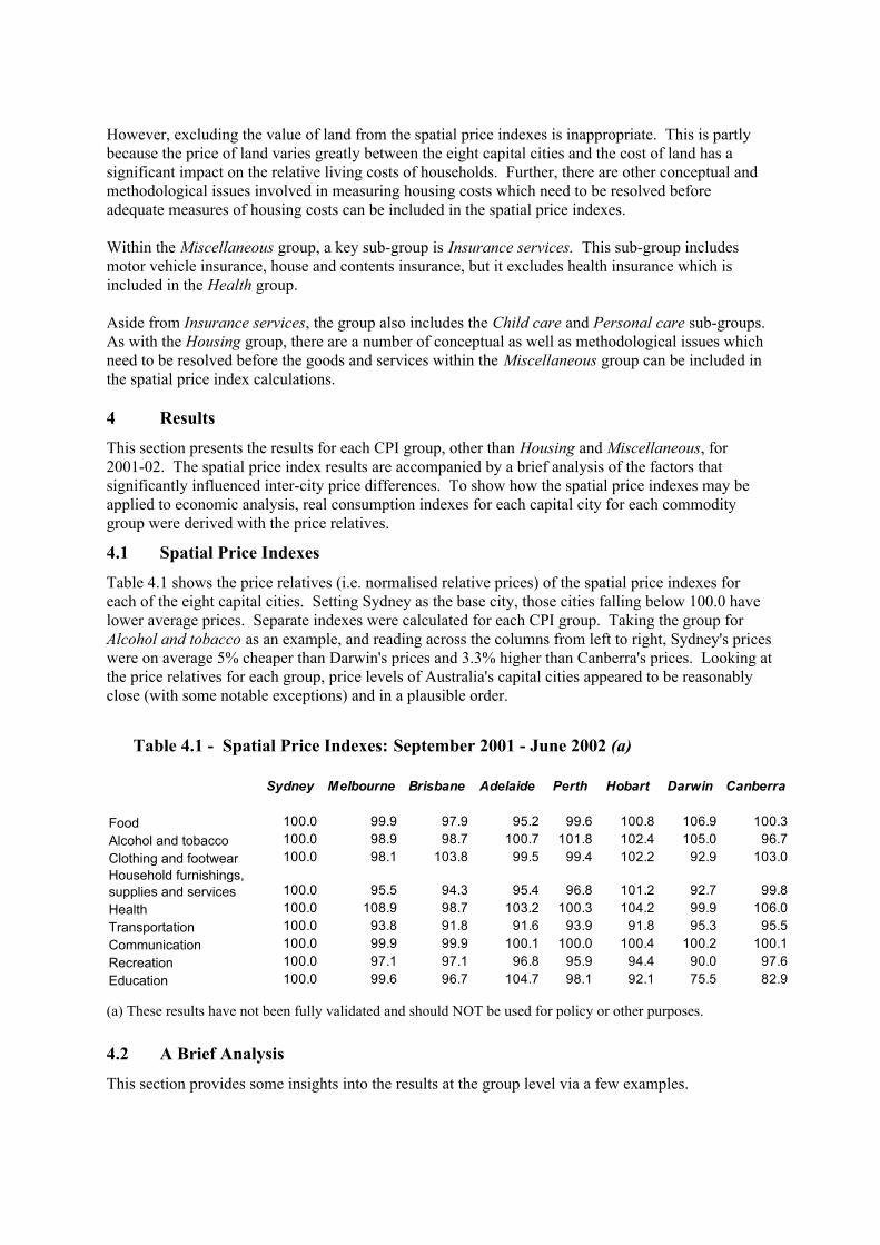
However, excluding the value of land from the spatial price indexes is inappropriate. This is partly because the price of land varies greatly between the eight capital cities and the cost of land has a significant impact on the relative living costs of households. Further, there are other conceptual and methodological issues involved in measuring housing costs which need to be resolved before adequate measures of housing costs can be included in the spatial price indexes.

Within the Miscellaneous group, a key sub-group is Insurance services. This sub-group includes motor vehicle insurance, house and contents insurance, but it excludes health insurance which is included in the Health group.

Aside from Insurance services, the group also includes the Child care and Personal care sub-groups. As with the Housing group, there are a number of conceptual as well as methodological issues which need to be resolved before the goods and services within the Miscellaneous group can be included in the spatial price index calculations.

4 Results

This section presents the results for each CPI group, other than Housing and Miscellaneous, for 2001-02. The spatial price index results are accompanied by a brief analysis of the factors that significantly influenced inter-city price differences. To show how the spatial price indexes may be applied to economic analysis, real consumption indexes for each capital city for each commodity group were derived with the price relatives.

4.1 Spatial Price Indexes

Table 4.1 shows the price relatives (i.e. normalised relative prices) of the spatial price indexes for each of the eight capital cities. Setting Sydney as the base city, those cities falling below 100.0 have lower average prices. Separate indexes were calculated for each CPI group. Taking the group for Alcohol and tobacco as an example, and reading across the columns from left to right, Sydney's prices were on average 5% cheaper than Darwin's prices and 3.3% higher than Canberra's prices. Looking at the price relatives for each group, price levels of Australia's capital cities appeared to be reasonably close (with some notable exceptions) and in a plausible order.

Table 4.1 - Spatial Price Indexes: September 2001 - June 2002 (a)

Sydney Melbourne Brisbane Adelaide Perth Hobart Darwin Canberra

Food 100.0 99.9 97.9 95.2 99.6 100.8 106.9 100.3Alcohol and tobacco 100.0 98.9 98.7 100.7 101.8 102.4 105.0 96.7Clothing and footwear 100.0 98.1 103.8 99.5 99.4 102.2 92.9 103.0Household furnishings, supplies and services 100.0 95.5 94.3 95.4 96.8 101.2 92.7 99.8Health 100.0 108.9 98.7 103.2 100.3 104.2 99.9 106.0Transportation 100.0 93.8 91.8 91.6 93.9 91.8 95.3 95.5Communication 100.0 99.9 99.9 100.1 100.0 100.4 100.2 100.1Recreation 100.0 97.1 97.1 96.8 95.9 94.4 90.0 97.6Education 100.0 99.6 96.7 104.7 98.1 92.1 75.5 82.9

(a) These results have not been fully validated and should NOT be used for policy or other purposes.

4.2 A Brief Analysis

This section provides some insights into the results at the group level via a few examples.

Transportation

Sydney's prices on transport were higher than in Adelaide (+8.4%), Perth (+6.1%), Darwin (+4.7%) and Canberra (+4.5%). The major price differences within this group were mainly attributable to the ECs for Other motoring charges and Urban transport fares. For example, Sydney's prices in the Other motoring charges EC were 54.1% higher than those in Canberra and 34.7% higher than in Perth. These gaps are wider than expected and will be examined further.

The Urban transport fares EC also showed significant price variations. Sydney came out 7.0% cheaper than Canberra and 6.1% cheaper than Melbourne. In contrast, it was more expensive than Hobart (by 40.9%), Darwin (by 34.8%), Perth (by 17.3%), Adelaide (by 16.3%) and Brisbane (by 6.8%).

For Melbourne, this difference may have been caused by the exclusion of (possibly cheaper) tram fares from our indexes. We could not calculate relative price differences for trams because this mode of transport was only available in one capital city. In Canberra, public transport fares were higher partly because they were measured on trips covering multiple zones.

Health

On average, Sydney's prices for health were lower than in Melbourne (-8.9%), Canberra (-6.0%), Hobart (-4.2%) and Adelaide (-3.2%). They were marginally higher than in Darwin (+0.1%) and Brisbane (+1.3%).

In Melbourne, higher health costs were mainly due to the higher prices in the Hospital and medical services EC (+15.8%). Canberra residents also paid more for their Hospital and medical services (+11.9%). In Canberra, this difference is because Canberra GPs tended to bulk bill less than those in other cities. As the index was calculated based on net costs (i.e. total costs net of government subsidies and rebates), the price information showed Canberra as being significantly more expensive than Sydney for a single GP consultation.

Further contributing to the overall health cost differences in Melbourne and Canberra were higher Dental services and Optical services. Melbourne residents paid 5.2% more for Optical services than their Sydney counterparts, whilst Canberrans paid 23.1% more. Canberrans also paid 21.8% more for Dental services than people living in Sydney.

Education

Education was cheaper in Sydney than in Adelaide (+4.7%) but significantly higher than Darwin (-24.5%) and Canberra (-17.1%).

Adelaide's higher prices were partly driven by secondary education fees, which were 14.1% above Sydney's. In contrast, Darwin recorded significantly lower prices in secondary education fees (-51%) as well as cheaper preschool and primary education fees (-48.5%). The relative prices for Darwin are lower than expected and we are still investigating the underlying causes for this. Two factors might have contributed to this difference, namely:

fewer services covered in Darwin; and/or,oDarwin containing more schools at the lower end of the price range. o

However, the sample specifications suggest that Darwin's prices covered a relatively similar range of education services. We are still examining this issue.

4.3 Per Capita Consumption Volumes by CPI Group

To demonstrate how the spatial price indexes may be used to derive other economic statistics, consumption volumes were calculated for each capital city. This section outlines these results and provides some interpretations.

Table 4.2 presents the indexes of the real weekly per capita consumption (or volume measures) for each of the eight capital cities for each group. Volume measures were derived by deflating the nominal weekly per capita expenditure figures with their price relatives. In this study, the nominal expenditure figures from the 1998-99 ABS Household Expenditure Survey were used. This is the most recently available expenditure data for each capital city. The analysis assumes that the relative price structures across the capital cities was the same in 1998-99 as observed in 2001-02. Appendix 4 provides further information on nominal and real per capita expenditures.

Table 4.2 - Real Per Capita Consumption Index 1998-99 (a)



(a) These results have not been fully validated and should NOT be used for policy or other purposes.

Price differences in some groups are worthy of further clarification. Initially, some of the relative price differences looked implausible. However, once these were cross-checked with information from other sources, the real per capita consumption (Table 4.2) figures seemed to reflect the situation on the ground. The information used in this analysis includes household and population characteristics published in the ABS publication HES: Summary of Results (ABS cat. no. 6530.0). A summary of the household and population characteristics is presented in Appendix 5.

Food

The price of Sydney's food was 4.8% higher than in Adelaide, but real weekly consumption was 8% higher in Sydney than in Adelaide. This gap can be put into context by examining Adelaide's household characteristics. For example, Adelaide had the lowest average weekly household income (at $797 compared with $1,022 in Sydney) and the number of people aged 65 years and over in a typical Adelaide household was the largest in the country (at 0.34). This suggests that the population in Adelaide is relatively older, which in turn suggests that they may tend to spend less on food than their Sydney counterparts.

In Hobart, the nominal per capita expenditure on food was $49.46, or 15.3% lower than in Sydney (See Appendix 4). But the price of food in Hobart is slightly higher than in Sydney (Table 4.1) and the gap between Hobart and Sydney (in real consumption terms) was 15.9%. This gap is surprisingly high and cannot be adequately explained by available demographic statistics and, as a result, needs further investigation.

Transportation

Our spatial price indexes indicate that Sydney had Australia's highest transportation costs (Table 4.1). The price differences between Sydney and the other capital cities ranged from 8.4% lower in Adelaide

to 4.5% lower in Canberra. At the same time, Sydney's residents on average spent $47.90 each on transportation in nominal terms (Appendix 4): 28% higher than in Adelaide ($34.20) and 14.5% lower than in Canberra ($54.80). The gaps in real consumption are smaller between Sydney and Adelaide (21.2%) but wider between Sydney and Canberra (19.9%).

The gap in real consumption between Sydney and Adelaide is reasonable, given that Sydney is geographically much larger than Adelaide. However, the big gap between Sydney and Canberra was unexpected -- Sydney's real consumption appeared to be too low in relative terms. This gap may be explained by the differences in the demographic structure of the two cities. For example, Sydney had a much larger proportion of older people than Canberra. According to HES: Summary of Results (Table 4, ABS cat. no. 6530.0.), the average number of persons per household was similar between Sydney (2.70 persons) and Canberra (2.56 persons). But, the number of persons aged 65 years and over was significantly higher in Sydney (0.31 or 11% of an average household) than in Canberra (0.19 or 7% of an average household). It is reasonable to expect that an older population consumes fewer transportation services.

Health

The nominal weekly per capita consumption of Sydney residents on health was, on average, $15.32 per week, while Canberrans each spent $15.39 per week (Appendix 4) on health. However, when these figures were converted into real consumption, Canberrans consumed about 5.2% less than Sydneysiders (Table 5.3). This gap may again be explained by Canberra's younger population.

Education

Darwin's education prices are another example where simply looking at the price relatives gives neither a realistic nor a complete picture. In this group, our spatial price index shows Darwin was 24.5% less expensive than Sydney (Table 4.1), partly because of lower preschool, primary and secondary education fees.

The information contained in HES: Summary Results (ABS cat. no. 6530.0) suggests that residents in Darwin spent significantly less on education than those in other capital cities, in nominal terms (Appendix 4). For example, they spent $5.02 per week on education, or 41.3% less than in Sydney ($8.56). When these numbers were converted into real weekly per capita consumption, the gap was significantly reduced. The real consumption for Darwin became $6.65 or 23.4% lower than in Sydney ($8.56). The discrepancy remains large, however, and this study is unable to provide an adequate explanation for the gap at the moment.

5. Summary and Future Research

This study explored the feasibility of developing experimental spatial price indexes in order to measure the price differences between Australia's eight capital cities. In this paper, indexes are presented at the group level, and their plausibility were examined by comparing real consumption figures (derived from the nominal expenditures and spatial price indexes) for the eight capital cities.

Most price observations in the CPI dataset appear to be suitable for comparisons between cities. However, the data for some services, such as "housing" and "miscellaneous" were found to be unsuitable, and therefore not included in the spatial price indexes at this stage.

Preliminary assessments are that the spatial price indexes look broadly plausible. For services such as "education", the index numbers for certain cities (e.g. between Sydney and Darwin) show wider gaps than expected, which we are unable to fully explain at the moment.

This paper reports our work-in-progress. We admit that the indexes are imperfect (particularly for services, such as health, transportation and education. We will improve the indexes in the future and would be grateful for readers' comments and suggestions on how we may be able to achieve this. In the meantime, readers are warned that the indexes are experimental in nature. As such, they should NOT be used for policy or for other purposes until the ABS validates the statistics and publishes them in an official publication.

The following two areas are considered important for future research:

Improving the quality of the service items currently covered - particularly for health, 1.transportation and education; andExpanding the coverage of the indexes to include Housing and some (or all) of the components 2.within the Miscellaneous group.

The ABS plans to release an information paper in early 2004. This paper will contain updated experimental estimates as well as "Total" indexes so that overall living costs between the capital cities can be compared. Further, the information paper will seek formal comment on the indexes as well as comments on how this project may be enhaned in the future.

Endnotes

1. In the PPP projects, this axiom is called Base-country invariance. A similar test in a time series index is called time reversal test.

2. Canberra�s bus zone system was recently replaced with a flat rate for all of Canberra. However, the data used for this study was for the 2001-02 year, which was before the new scheme was introduced.

Appendix 1: EKS Spatial Price Index formula

The Multilateral EKS index was proposed by Gini (1931), Elteto and Koves (1964) and Szulc (1964) and it is an extension of the bilateral Fisher index. An EKS price index between cities k and b involving J cities in the comparison can be expressed as:

( )1/

1

JJF Fk

kb jk bjjb

PI P PP =

= = ×∏(A1.1)

where Pi ( Π ) is a multiplication sign and FjkP

and F

bjP are the Fisher indexes (Equation A1.2).

( )

1/ 2

1/ 2 1 1

1 1

I I

ki bi ki kiF Las Paas i i

kb kb kb I I

bi bi bi kii i

p q p qP P P

p q p q

= =

= =

= × = ×

∑ ∑

∑ ∑(A1.2)

In Equation (A1.2), the first component in the bracket is called Laspeyres index and the second component Paasche index. For example, in a price comparison involving Sydney (s), Melbourne (m) and Darwin (d), the index between Sydney and Melbourne is given by:

( )( )( )( )1/ 3F F F F F Fssm ss ms ds md ms mm

m

PI P P P P P PP

= = × × ×

or

( )( )1/3F F F Fssm ms ds md ms

m

PI P P P PP

= = × × ×(A1.3)

since F

ssP and F

mmP are always equal to 1. This expression is formed using 3 pairs of bilateral Fisher indexes for the 3 cities under investigation.

Appendix 2: Statistical Properties of a Multilateral Index

In the literature, axiomatic tests have been used to examine the statistical properties that lead to index formulas giving satisfactory results. This approach tests indexes against a predetermined set of statistical criteria (axioms): good indexes are expected to pass important tests. Diewert (1986) suggests more than two dozen axioms for multilateral indexes. In this paper, the focus was on 4 tests considered most important for our purposes. These axioms are:

transitivity (or circularity);oconsistency in aggregation;ofactor reversal; andobase-city invariance.o

Transitivity

The EKS index satisfies the transitivity test (Box A2.1). Transitivity ensures that the indexes are internally consistent across the different locations under investigation. It avoids potential confusion which may otherwise occur as a result of inconsistent index numbers being derived, when cities are compared directly or with a third city. It is a desirable property when the spatial price indexes are used for a variety of purposes.

Box A2.1 Transitivity Test

If a spatial price index is transitive, a consistent result will be achieved whether prices are compared directly between two cities or indirectly through other cities. For example, when comparing Sydney (s) , Melbourne (m) and Darwin (d), the spatial index will be transitive if the following condition holds:

sm sd dmI I I= × (A2.1)

where smI is the index for Sydney and Melbourne, sdI is the index for Sydney and Darwin and

dmI is the index for Darwin and Melbourne.

Consistency in Aggregation

Consistency in aggregation ensures indexes are internally consistent between the different aggregation levels (Box A2.2). Again, this is another desirable property for our spatial price indexes. Unfortunately, the EKS index does not satisfy this test.

Box A2.2 Consistency in Aggregation

A spatial price index is consistent in aggregation if an aggregate index can be derived exactly from its sub-indexes (i.e. indexes at the lower aggregation levels). For example, if the spatial price index between Sydney and Melbourne covers two components (i.e. food and clothing), then in a very simple case, this index is consistent in aggregation, if the following condition holds:

(1 )F Csm sm smI wI w I= + − (A2.2)

where f

smI and csmI are the component indexes for food and clothing and w and 1-w are weights.

Factor Reversal Test

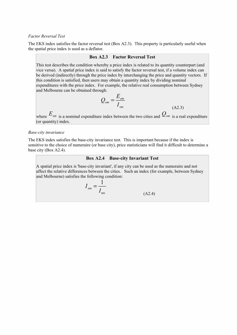
The EKS index satisfies the factor reversal test (Box A2.3). This property is particularly useful when the spatial price index is used as a deflator.

Box A2.3 Factor Reversal Test

This test describes the condition whereby a price index is related to its quantity counterpart (and vice versa). A spatial price index is said to satisfy the factor reversal test, if a volume index can be derived (indirectly) through the price index by interchanging the price and quantity vectors. If this condition is satisfied, then users may obtain a quantity index by dividing nominal expenditures with the price index. For example, the relative real consumption between Sydney and Melbourne can be obtained through:

smsm

sm

EQI

=(A2.3)

where smE is a nominal expenditure index between the two cities and smQ is a real expenditure (or quantity) index.

Base-city invariance

The EKS index satisfies the base-city invariance test. This is important because if the index is sensitive to the choice of numeraire (or base city), price statisticians will find it difficult to determine a base city (Box A2.4).

Box A2.4 Base-city Invariant Test

A spatial price index is 'base-city invariant', if any city can be used as the numeraire and not affect the relative differences between the cities. Such an index (for example, between Sydney and Melbourne) satisfies the following condition:

1sm

ms

II

=(A2.4)

Appendix 3: Index Construction Method

To apply the generic EKS formula (Equation A1.1) to our spatial price indexes, we needed to use expenditure weights. In the CPI dataset, most weights are available only at EC level and above. Consequently, we had to slightly modify the EKS formula in order to apply it to the levels below the ECs.

Within the CPI a standard practice is to use a geometric mean when expenditure weights are not available. At the EA level, the geometric mean (between locations k and b) is defined as:

1/ IIki

kbi bi

pJp

=

∏

(A3.1)

where kip and bip stand for the prices of commodity i sold in locations k and b respectively, Pi ( Π

) is a multiplication sign, (

ki

bi

pp ) is the price relative for commodity i and I is the total number of

commodities.

Our spatial price indexes are constructed based on two variants of the EKS index. Below the EC level, it looks like this:

( )1/

1

JJk

kb jk bjjb

PI J JP =

= = ×∏(A3.2)

Whilst at the EC level and above, we used the normal EKS formula defined in Equation A1.1.

Appendix 4: Nominal and Real Per Capita Expenditures

Nominal Per Capita Expenditures by group: 1998-99 (a)Sydney Melbourne Brisbane Adelaide Perth Hobart Darwin Canberra

($) ($) ($) ($) ($) ($) ($) ($)


(a) the nominal expenditure figures were obtained from the 1998-99 Household Expenditure Survey

Nominal Per Capita Expenditures Index by group: 1998-99 (a)Sydney Melbourne Brisbane Adelaide Perth Hobart Darwin Canberra


(a) the nominal expenditure figures were obtained from the 1998-99 Household Expenditure Survey

Real Per Capita Expenditures by Group: 1998-99 (a) (b)Sydney Melbourne Brisbane Adelaide Perth Hobart Darwin Canberra

($) ($) ($) ($) ($) ($) ($) ($)


(a) Derived by deflating the 1998-99 nominal expenditures by the 2001-02 spatial indexes. This assumes that the observed price relatives in 2001-02 were present in 1998-99.(b) These results have not been fully validated and should NOT be used for policy or other purposes.

Appendix 5: Household Characteristics of the Eight Capital Cities, 1998 - 99


All capitalcitiy

householdsAverage weekly household income ($) 1 021.54 1 010.51 843.61 797.49 889.26 807.53 1 196.07 1 137.05 957.17

Average number of persons in the household Under 18 years 0.65 0.65 0.67 0.55 0.6 0.68 0.9 0.67 0.64 18 to 64 years 1.73 1.77 1.64 1.47 1.63 1.58 2.00 1.69 1.69 65 years and over 0.31 0.29 0.26 0.34 0.25 0.28 0.09 0.19 0.29 Total 2.70 2.70 2.57 2.37 2.48 2.55 2.99 2.56 2.62

Household composition (% of households) Couple, one family Couple only 22.7 24.7 22.3 24.0 20.0 23.2 22.2 24.0 23.0 Couple with dependent children only 24.1 23.9 24.9 19.8 21.6 23.0 34.5 26.7 23.6 Other couple, one familyhouseholds 12.8 15.1 10.1 10.0 13.5 9.5 10.2 8.7 12.7 One parent, one family with dependent children 4.9 6.5 8.1 6.8 6.8 9.7 8.7 5.7 6.3 Other family households 8.9 5.2 6.1 3.8 4.7 3.9 5.6 3.3 6.2 Lone person 21.9 21.8 24.9 30.5 30.2 26.5 13.2 24.1 24.2 Group 4.7 2.9 3.6 5.0 3.2 4.2 5.6 7.4 4.0 Total 100.0 100.0 100.0 100.0 100.0 100.0 100.0 100.0 100.0

Estimated number in population ('000) Households 1 461.9 1 246.3 613.3 448.1 535.3 78.6 31.4 118.1 4 533.0 Persons 3 940.1 3 367.6 1 573.2 1 060.1 1 328.8 200.3 93.8 301.7 11 865.5Number of households in sample 1 327 992 580 420 475 389 335 277 4 795

Source: Table 4, HES: Summary Results, ABS Cat. 6530.0.Note: The figures were derived from the 1998-99 Household Expenditure Survey.

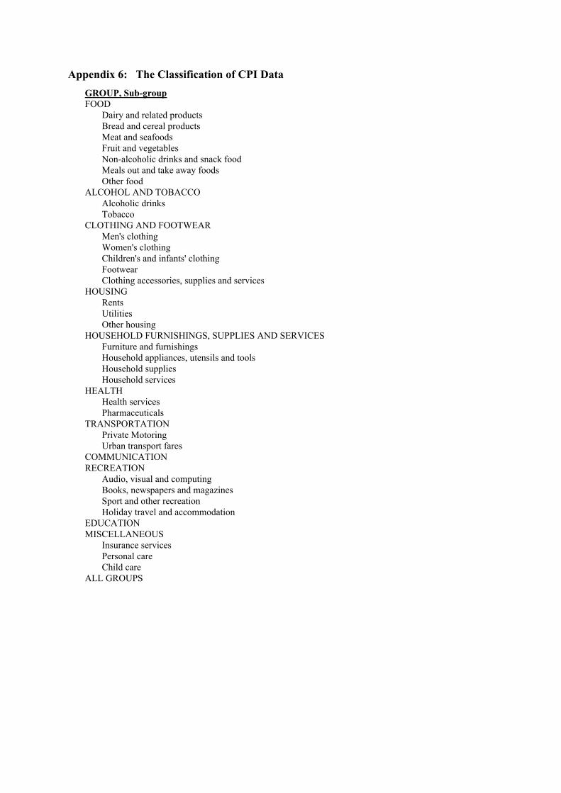
Appendix 6: The Classification of CPI DataGROUP, Sub-groupFOOD

Dairy and related productsBread and cereal productsMeat and seafoodsFruit and vegetablesNon-alcoholic drinks and snack foodMeals out and take away foodsOther food

ALCOHOL AND TOBACCOAlcoholic drinksTobacco

CLOTHING AND FOOTWEARMen's clothingWomen's clothingChildren's and infants' clothingFootwearClothing accessories, supplies and services

HOUSINGRentsUtilitiesOther housing

HOUSEHOLD FURNISHINGS, SUPPLIES AND SERVICESFurniture and furnishingsHousehold appliances, utensils and toolsHousehold suppliesHousehold services

HEALTHHealth servicesPharmaceuticals

TRANSPORTATIONPrivate MotoringUrban transport fares

COMMUNICATIONRECREATION

Audio, visual and computingBooks, newspapers and magazinesSport and other recreationHoliday travel and accommodation

EDUCATIONMISCELLANEOUS

Insurance servicesPersonal careChild care

ALL GROUPS

ReferencesABS (1995) Spending and income, Christmas Island and the Cocos (keeling) Island , Australian Bureau of Statistics, ABS Cat. No. 6552.0.

ABS (2003) Australian Consumer Price Index: Concepts, Sources and Methods, ABS Cat 6461.0, Australian Bureau of Statistics.

Biggeri, Luigi (1998) "Consumer price indices: purposes and definitions: a useful general approach to the construction of the indices and some measures of the divergences between them", Proceedings of the Fourth Meeting of the International Working Group on Price Indices, US Department of Labour, Bureau of Labour Statistics, Washington DC, April 22-24, 1998.

Balk, Bert M. (1996) "A comparison of ten methods for multilateral international price and volume comparison", Journal of Official Statistics, Vol. 12, No. 2 1996, pp. 199 - 222.

Caves, D. W., L. R. Christensen and W. E. Diewert (1982) "Multilateral comparisons of output, input and productivity using superlative index numbers", Economic Journal, Vol. 92, pp. 73-87.

Cuthbert, James R. (1999) "Categorisation of additive purchasing power parities", Review of Income and Wealth, 45, pp 235 - 249.

Cuthbert, James R. (2000) "Theoretical and practical issues in purchasing power parities illustrated with reference to the 1993 Organisation for Economic Co-operation and Development Data", Journal of Royal Statistical Society A (2000), 163, Part 3, pp 421-444.

Diewert, W. E. (1976) "Exact and superlative index numbers", Journal of economics, Vol. 44, No. 3 (May 1976), pp. 115 - 45.

Diewert, W. E. (1986) "Microeconomic approaches to the theory of International Comparisons", Technical Working Paper No. 53, Cambridge MA: National Bureau of Economic Research. Abridged version entitled "Test Approaches to International Comparison", in Eichorn W. (1988) ed. Measurement in Economics, Heidelberg: Physica-Berlag and in Diewert and Nakamura (1993) eds. Essays in Index Number Theory, Volume 1, Amsterdam: North-Holland.

Diewert, W. E. (1987) "Index Numbers", in J. Eatwell, M. Milgate and P. Newman (eds) New Pagrave Dictionary of Economics (Vol. 2), New York: Stockton, Press, pp. 767-780.

Dreschsler L. (1973) "Weighting of Index Numbers in Multilateral International Comparison", Review of Income and Wealth, Ser 19, No. 1, 17 - 34.

Elteto, O. and P. Koves (1964) "On a problem of index number computation relating to international comparison, Statisztikai Szemle, 42, pp. 507-18.

Geary R. C. (1958) "A note on comparisons of exchange rates and purchasing power between countries", Journal of the Royal Statistical Society, Series A, 121, pp. 97-99.

Gini C. (1931) "On the circular test of index numbers", International Review of Statistics, Vol. 9., No. 2, 3 25,

Hill, Robert (1997) "A taxonomy of multilateral method for making international comparisons of prices and quantities", Review of Income and Wealth, Series 43, No. 1, March 1997, pp. 49 -69.

ILO (2001), "International Labour Organisation CPI Manual (v2)", www.ilo.org/publish/english/bureau/stat/download

Khamis, S. H. (1972) "A new system of index numbers for national and international purposes", Journal of the Royal Statistical Society, Series A, 135, pp. 96-121.

Khmais S. H. (1984) " On Aggregation Methods for International Comparisons". The Review of Income and Wealth, 30, 195 - 205

Kokoski M. F. (1987) "Problem in the measurement of consumer cost of living indexes". Journal of Business & Economic Statistics, 5, 39-46.

Kokoski, M. F. Cardiff, P. and Moulton B. R. (1994) "Interarea Prices for Consumer Goods and Services: An Hedonic Approach Using the CPI data", Working Paper 256, US. Department of Labour, Bureau of Labour Statistics.

Kokoski, M. F. Moulton, B. R., and Ziechang, K. D. (1996) "Interarea Price Comparisons of Heterogeneous Goods and Several Level of Commodity Aggregation," Working Paper 291, US. Department of Labour Bureau of Labour Statistics.

Koo, Jahyeong, Keith R. Phillips and Fiona D. Sigalla (2000) "Measuring Regional Cost of Living", Journal of Business & Economics Statistics, Vol. 18. No. 1, pp. 127-136.

Kravis, I. B., Heston, A., and Summers R. (1978) International Comparisons of Real Product and Purchasing Power, Baltimore, MD: Johns Hopkins University Press.

Kravis, I. B., Heston, A., and Summers R. (1982) World Product and Income: International Comparisons of Real Gross Product, Baltimore, MD: Johns Hopkins University Press.

Kravis, I. B., Kenessey, Z., Heston, A., and Summers R. (1975) A System of International Comparisons of Gross Product and Purchasing Power, Maltimore, MD: Johns Hopkins University Press.

Moulton, B. R. (1995) "Interarea indexes of the cost of shelter using hedonic quality adjustment techniques", Journal of Econometrics, 68, pp. 181-204.

OECD (1993) Purchasing Power Parities and Real Expenditures, Statistics Directorate, Organisation for Economic Co-operation and Development 1993.

Pollak, R. A. (1989) The Theory of the Cost of Living Index, New York: Oxford University Press.

Stott, Helen (1998) "The CPI purpose and definition - the Australasian debate", Proceedings of the Fourth Meeting of the International Working Group on Price Indices, US Department of Labour, Bureau of Labour Statistics, Washington DC, April 22-24, 1998.

Szulc B. (1964) "Indices for multiregional comparisons", Przeglad Statystyezny 3, Statistical Review 3, pp. 239-54.

United Nations (1986). World comparisons of Purchasing Power and Real Product for 1980. New York: United Nations

United Nations (1992). Handbook of the International Comparison Programme. Studies in Methods Series F. No. 62. New York: United Nations.

Pollak, Robert (1983) "The Theory of the Cost-of-Living Index", in W. E. Diewert Price Level Measurement: Proceedings from a Conference Sponsored by Statistics Canada, pp. 87-162, Published under the authority of the Minister of Supply and Services Canada.

Van Ijzreren (1983) "Index numbers for binary and multilateral comparison: algebraical and numerical aspects", Statistical Studies, No. 34. The Hague: The Netherlands Central Bureau of Statistics.

Van Ijzeren (1987) Bias in international index numbers: a mathematical elucidation, Eindhoven: CIP-Gegevens Koninklijke Bibliotheek.

comparing living costs in australian capital cities · 2008-09-09 · comparing living costs in...

Documents