Comparing Four Secular Home Price IndicesJacques Friggit1

Working paper, version 92, June 2008

AbstractWe compare four secular home price indices, focusing more on the methods than on the results and asking rather more questions than we bring answers.Differences in perimeter, method and urban and social evolutions impact the values of the indices, in ways which we cannot always measure. Therefore, their comparison is difficult, and their long term trends should be interpreted with caution.On the other hand, the temporary ups and downs of the indices clearly show the impact of some major historical events.

1. The four secular indices 31.1. Herengracht index since 1628 (Eichholtz, 1994) 31.2. Paris indices since 1200 (d’Avenel, 1894), and since 1790 and 1840 (Duon, 1946) and (Friggit, 2001) 3

1.2.1. Prior to 1790: d’Avenel 31.2.2. 1790-1850 and 1840-1944: Gaston Duon 41.2.3. 1944-1999: index based on the price of the previous transaction mentioned in Notaries’ databases 91.2.4. Since 1999: Notaires-INSEE index 10

1.3. Norwegian main city index since 1819 (Eitrheim & Erlandsen, 2004) 111.3.1. 1819-1985: weighted repeat sales 111.3.2. Since 1986: house price per square meter 11

1.4. US index since 1890 (Grebler, Blank and Winnick, 1956) and (Shiller, 2005) 111.4.1. 1890-1934: Grebler, Blank and Winnick 111.4.2. 1934-1953: average of advertised median prices over 5 cities 121.4.3. 1953-1975: home purchase component of the US consumer price index 121.4.4. 1975-1987: OFHEO’s repeat sales index 121.4.5. Since 1987: S&P/Case-Shiller National index 12

2. Comparison: methods 132.1. Main features 13

2.1.1. Areas covered 132.1.2. Dwellings covered 132.1.3. Source of the price 132.1.4. All four indices are at least in large part repeat sales indices 132.1.5. Pure or composite? 14

2.2. In their repeat sales part, all four indices make little adjustment for quality beyond the obvious and beyond Duon’s and Grebler’s global adjustments 14

2.2.1. Building use 142.2.2. Physical improvements 142.2.3. New dwellings 142.2.4. Adjustment for obsolescence or depreciation 15

2.3. Hard to measure changes in the urban and social status of their perimeter impact the indices 152.3.1. Urban evolution 152.3.2. Social evolution 16

3. Comparison: results 173.1. 1200-1628 19

3.1.1. Long term trend 193.1.2. Impact of major events 19

3.2. 1628-1820 203.2.1. Long term trend 203.2.2. Impact of major events 20

3.3. 1820-1900 203.3.1. Long term trend 213.3.2. Impact of major events 21

3.4. 20th century 223.4.1. Long term trend 22

1 Conseil Général des Ponts et Chaussées, Ministry of Ecology, Sustainable Planning and Development, Paris, France.2 Version 9 differs from versions 7 and 8 only concerning d’Avenel’s average Paris home prices prior to 1800 (in particular, in this version we use d’Avenel’s consumer price index to deflate his home price index). Cf. 1.2.1, 1.2.2.5, 3.2.2 and the appendix.

1

3.4.2. Impact of major events 243.5. Home price indices compared to income per household or proxies 27

4. Conclusion 29Appendix: data and sources 30

2

1. The four secular indices We present here the four indices in the chronological order of their publication.The Herengracht index and the Norwegian main city index are described in a quite detailed way by the very persons who calculated them in papers easily available on the web; therefore, we will describe these indices only shortly and refer the reader to these papers for more details.On the contrary, parts of the Paris and of the US index are based on indices produced a long time ago (the 1940’s in the former case, the 1950’s in the latter case) and described in paper documents available only in a few libraries; therefore, we will comment these parts of these indices in more detail.

1.1. Herengracht index since 1628 (Eichholtz, 1994) The construction of this index is described in “A Long Run House Price Index: The Herengracht Index, 1629-1973”, Piet M.A. Eichholtz, University of Limburg, Maastricht and University of Amsterdam, Amsterdam, August 1996.It covers, on a biennial basis, 4873 properties located along the banks of the Herengracht, a canal in Amsterdam. In the Golden Age of this city, the 17 th century, this area was the most fashionable place in the Netherlands. It was urbanized very early: by 1680 nearly all the lots along the canal had been developed.The index was built using a repeat sales method by comparing the successive sale price of buildings.4252 transaction prices for the 1628-1973 period were collected, say on average 12.3 prices per year.The only quality taken into account is the use of the buildings. Beginning in the 19 th century, but especially in the 1920’s and 1930’s, many buildings along the Herengracht were changed into offices, which increased their value. Buildings used as offices have been excluded from the calculation.All other quality effects have not been filtered out. Thus, if for instance central heating was installed between two successive transactions, the resulting effect of this amenity on the price is not filtered out.

1.2. Paris indices since 1200 (d’Avenel, 1894), and since 1790 and 1840 (Duon, 1946) and (Friggit, 2001)

We use here:- d’Avenel’s series of home prices in the centre of Paris from 1200 to 1800,- Duon’s 1625-1850 index for the centre of Paris (cf. 1.2.2.5), which itself uses d’Avenel’s series for 1625-

1790,- and the index since 1840 described in « Reconstitution des prix immobiliers passés à partir des bases de

données notariales et de la série de Gaston Duon, note méthodologique » (« reconstitution of past property prices based on Notaries’ databases and Gaston Duon’s series, methodological note»), Jacques Friggit, working paper, unpublished, January 2002, 49 pages, which is built by connecting Duon’s 1840-1944 index, an index we built on 1944-1999 and the Notaires-INSEE index since 1999.

1.2.1. Prior to 1790: d’Avenel Based on transaction prices he collected, d’Avenel4 provides a series of average home prices (averaged over 25-year periods) from 1200 to 1800 in Paris, which in this case means a more and more extended area in the centre of the present city of Paris. He provides similar series for “towns outside of the Paris region” and for “villages”.He expresses the prices in a currency unit consisting in Francs supposed to contain 4.5 grams of silver.In addition, d’Avenel provides an index of the ”purchasing power” (with respect to the general expenses of the population) of his currency unit, so that a “constant currency” home price series can be calculated.

During such a long period of time, the quality and the structure of the housing stock and of the houses sold changed extensively. Thus d’Avenel’s series is not at all a “constant quality” one. D’Avenel was fully aware of that and comments extensively on it. The same remark applies to the series of the purchasing power of the currency unit.Therefore, and although d’Avenel tried in some measure to correct his index for changes in the structure of the houses sold, this series can only be considered with caution, and used in full knowledge of the way it is calculated (in particular, contrary to the other long-term home price indices compared here, it is not a repeat sale index) and of its limits.

3 487 presently, as opposed to 614 originally, this decrease stemming from the combination of lots to allow for the construction of bigger buildings.4 Georges d’Avenel (1855-1939) began working with the French government, then mostly studied historical economy. Among other works, he wrote an “Economic History of Property, Salaries, Foodstuff, and All Prices in General from Year 1200 to Year 1800” (cf. appendix), based on the collection and analysis of “seventy-five thousand” prices of various items and prized by the Academy of Moral and Political Sciences.

3

Chart 1 : d’Avenel’s series, 1200-1800, nominal silver currency

D'Avenel's seriesCentre of Paris

Nominal silver currency

100

1 000

10 000

100 000

1200 1300 1400 1500 1600 1700 1800

Average house pricein silver Francs

1.2.2. 1790-1850 and 1840-1944: Gaston Duon It seems that Duon5 pioneered repeat sales home price indices6.During WWII, while working with the French statistical office, by comparing the successive transaction prices of Parisian properties gathered from the property registers kept by the Tax Department he calculated yearly home price indices for Paris for years 1840-1944. In addition, by the same method, he calculated a home price index for the centre of Paris by 10- year periods for years 1790-1850.

1.2.2.1. SourcesDuon’s work is presented in three papers:

- « Évolution de la valeur vénale des immeubles parisiens »(« Evolution of the selling price of Parisian buildings »), Journal de la Société de Statistique de Paris, octobre 1943, pages 169-192.

- « Évolution de la valeur vénale des immeubles à Paris de 1840 à 1939 » (« Evolution of the selling price of buildings in Paris from 1840 to 1939 »), Bulletin statistique de la France, décembre 1943, pages 375-378.

- « Documents sur le problème du logement » (« Documents on the problem of housing »), Études Économiques, 1946, n°1, pages 1 to 165.

The first paper describes the data and details the methodology, including the main problems encountered, the solutions chosen and the mathematical formulas used in absence of computers. It also provides a first set of results7.The second paper merely summarizes the first one.5 Gaston Duon (1908-2005) worked with the French statistical office, the United Nations (including a stay in New York in the early 1950’s), Eurostat and Brussels University (source: Mrs. Monique Duon). In spite of his stay in the USA, his work about Paris home prices seems to have remained unknown in that country (cf. note Error: Referencesource not found).6 (Grebler, Blank and Winnick, 1956) (cf. 1.4.1) mentions in Appendix C that “no national house price index covering a reasonably long period of time exists, although house price indices have been constructed for several cities, usually covering a relatively few years” and quotes in a footnote two indices predating Duon’s papers: one for Ann Arbor (Hermann Wyngarden, An Index of Local Real Estate Prices, University of Michigan School of Business Administration, Bureau of Business Research, 1927) and one for Toledo (William Hoad, “Real Estate Prices”, unpublished doctoral dissertation, University of Michigan, 1942). We didn’t look at these two works, but, since they cover “relatively few years”, the likelihood that they are based on a repeat sales method is limited. (Grebler, Blank and Winnick, 1956) does not mention Duon’s work.7 At the end of this paper is also a transcript of its discussion by Duon’s peers at Société de Statistique de Paris. It shows that linear regressions was not unknown of them. One of Duon’s colleagues, Hénon, proposed to use “the method of correlations”, “partial and total correlations”, “analysis of variance”. Hénon also mentioned Roos’ work about construction demand in the USA published in Dynamic Economics (Cowles Commission, 1934, http://www.econ.yale.edu/cowles/P/cm/m01.htm) as a possible source of inspiration for additional work.

4

The third paper recalls the methodology but mostly provides extended results. These results are different from those presented in the first paper (although they are similar), which suggests that in the meantime more data had become available or that the methodology had been improved.The third paper mentions that another paper “in preparation”, titled “Enquêtes diverses sur les immeubles et les logements à Paris”, will provide the method of the calculations and the details of the analysis of the data. We couldn’t find it in spite of searches in various archives. Nevertheless, the first and third papers provide enough information about the data and the method for us to understand most of Duon’s calculations. The details below stem from these papers, except when mentioned otherwise.

1.2.2.2. Perimeter of the indices (1840-1944)Duon provides price indices for whole rented buildings (“maisons de rapport”), apartments and detached houses (which he calls “hôtels particuliers” or “pavillons”), and land. He also provides rent indices and (for the 1914-1944 period) a total return (i.e., including reinvested rent net of expenses) index.There are very few detached houses in Paris; in addition, no apartment was owned or sold by the unit prior to WWI and very few were in the interbellum period. Therefore, we used Duon’s index for whole rented buildings. This index is representative of the price of the homes of almost all Parisians, since in 1944 only 3% of Parisian households owned their home.Duon mentions in his 1943 paper that around 1100 rented buildings (against 400 apartments sold by the unit) are sold every year. In his 1946 paper he uses 1129 sales of rented buildings occurred in 1941, 1277 occurred in 1942, 1215 occurred in 1943 and 768 occurred in 19448. He excludes special types of sales such as auctions9

(forced or not), etc.10

He provides extensive data about rented buildings in Paris, of which we quote the following:- the average surface of the buildings sold was 340 square meters in 1939 and 366 square meters in 1944;- the average number of rooms per dwelling was almost the same in 1891 and in 1936 (2.6);- the average number of persons per building was 27 in 1862, 33 in 1914 (since the average size of the buildings increased in the meantime, one should not conclude that the number of persons per room increased) and 31 in 1944;- the average number of households per building was 13 in 1851 and 14 in 1914 (same remark);- in 1891, 85% of buildings had running water, against 98% in 1944; nevertheless the tap could be common to several dwellings: in 1944, only 80% of dwellings had individual running water;- in 1891, 25% of dwellings had individual toilets, against 46% in 1944.These data show that comfort grew sharply during the period covered by Duon’s indices.

In 1944, rented buildings had an average age of 65 years. Their numbers per year of construction are shown in table 1. One can see that in 1944, fewer than 30% of multi-family buildings (i.e., buildings covered by Duon’s rented building index) had been build prior to 1851.

Table 1 : Number of buildings used as dwellings per year of construction and type.Buildings used as dwellings, 1942

BourgeoisSemi-

bourgeois Workers BourgeoisSemi-

bourgeois Workers

Before 1851 167 207 250 1 107 5 266 14 277 2 136 1 462 46 22 920 27%1851-1880 566 432 786 2 102 5 790 13 862 399 1 084 27 25 048 30%1881-1914 632 677 1 055 3 605 6 288 13 704 12 530 1 029 62 27 594 33%1915-1942 343 545 571 1 511 2 702 2 545 12 98 370 12 8 709 10%Total 1 708 1 861 2 662 8 325 20 046 44 388 26 1 163 3 945 147 84 271 100%% 2,0% 2,2% 3,2% 9,9% 23,8% 52,7% 0,0% 1,4% 4,7% 0,2% 100,0%

Period of construction

Business with a few dwellings

Craftman's with a few dwellings

Total %One-family building Multi-family building Workers'

tenement

Castle and exceptional

house

8 As far as we understand, Duon used almost all the sales by mutual consent occurred in Paris. 9 In 1939, auctions represented 3.5% of property sales in Paris.10 We have no proof that the special circumstances of these years might have impacted the types of buildings sold. We tried to assess whether Duon’s index was significantly impacted by sales which (for racial, political or other motives) were either openly forced, or in practice forced but disguised as sales by mutual consent. Duon explicitly mentions that he excluded auctions. Since he knew the nature of the sale, we believe he excluded from his sample other sales which were openly forced. We tried to extrapolate elements kindly provided to us by Claire Andrieu, from Institut d’Études Politiques de Paris (including her student Johanna Mouyal’s 2004 mémoire de maîtrise). We could not reach a reliable enough conclusion, which only more work could bring.On the contrary, there are concordant reports of considerable price dissimulation during and after WWII to evade transaction taxes (which amounted to 17% to 36% of the price during the Occupation and were still very high in the following years) and to launder black or grey money, particularly abundant in that troubled period and its aftermath.A comparison with what happened in the Herengracht area or in Norway’s main cities in these respects during this period might be interesting. As far as forced sales are concerned, a starting point could be “Spoliation et restitution des biens juifs en Europe au XXe siècle” (C. Goschler, P.Ther & C. Andrieu, published by Autrement, 2007, translated and updated from original German and English versions), which provides many references.

5

Duon’s series on 1840-1944 cover all of Paris in its current borders11.While a specificity of France is that its population grew very slowly from 1840 to 1940, Paris’ population almost trebled in that period. The population of Paris grew much faster than France’s prior to the 1920’s, then slower; it even decreased in the most recent decades12.

Table 2 : population, France and ParisPopulation in thousandYear France ( in its current borders) Paris (in its current borders) Paris / France

1840 35 421 1 049 3%1860 37 943 1 665 4%1880 39 804 2 213 6%1900 41 329 2 679 6%1920 40 069 2 905 7%1940 41 865 2 750 7%1960 46 782 2 809 6%1980 55 173 2 211 4%2000 60 751 2 140 4%2006 63 195 2 155 3%

Source: INSEE.

Paris is administratively divided into 20 “arrondissements”. Duon grouped them into 5 “districts”, the yearly number of transactions of rented buildings in each district being approximately the same (around 200) in his time. For the 1880-1914 period, in addition to his index for all of Paris, Duon provides an index (before adjustment for obsolescence, see below) for each “district”. He mentions that, due to the small number of records, the yearly value of these indices is not very reliable and that only their trend should be considered. The growth in these indices highly depends on the group considered (cf. chart 2 and chart 3).

1.2.2.3. Data (1840-1944)For rented buildings, the property register used by Duon contained the following information:

- number of buildings,- number of floors,- building facing a yard, dead-end,- existence of cellars or underground floor,- existence of an elevator,- materials used for the roof,- materials used for the construction,- “importance” of rents,- date of construction,- surface,- sale price,- “nature” of the sale (which we understand means by auction or not, by mutual consent or forced, etc.),- “income” of the building (rent, minus some expenses).

Duon excluded pairs of transactions between which the building had undergone a transformation, as far as this information was available13. Besides that, he didn’t take into account changes in the quality of buildings, including their use14, except for his global “adjustment for obsolescence” (cf. below).

1.2.2.4. Description of the calculations (1840-1944)First, Duon considered buildings sold around 194115 (in 1939 in the 1943 papers). By comparing their price in that year to their price in former years, back to 1840, (what he calls “triangulation”) he built an first index16.Then, he considered buildings sold at intervals of 20 years:

11 Prior to 1860, Paris did not include what are now its peripheral districts, such as Montmartre.12 Contrary to other large cities such as New York City or London, Paris does not include its suburbs.13 So we may infer that pairs of transactions between which an elevator had been installed were excluded.14 Nevertheless, although many of the “maisons” or “immeubles de rapport” considered may very well have included shops in the ground floor, they were mostly residential.15 From the 1946 paper, it is not completely clear to us whether only buildings sold in 1941 were considered, or whether buildings sold in other recent years were also considered, but the second option seems the most likely. How he calculated the indices for the 1940’s is not completely clear to us, although he seems to have compared the price of buildings purchased in the same year (for instance, 1914) and resold in 1941, 1942, 1943, etc.16 He calculated the truncated average (each building counting for 1) of the ratios: current price / former price, excluding in each district the 25% largest and the 25% smallest ratios. He mentions that he also tried the ratio: sum of current prices / sum of former prices, truncated the same way, that it provided very similar results, and that consequently he chose the former calculation because it was easier. His 1943 paper mentions that the averages were calculated on rolling 3-year periods after WWI and 5-year periods prior to WWI. It’s not clear to us whether the series published in his 1946 paper is smoothed too. Finally, the index is calculated as the inverse of this series.

6

- both in 1858-1862 and 1880,- both in 1878-1882 and 1900,- both in 1898-1902 and 1920,and he found that the price increase measured on these pairs of transactions was 20% larger than the increase in the index just mentioned.In his 1943 paper, he also compared the price of buildings located in the same districts and built in different periods, and observed that buildings built in a given period were losing around 20% of their value every 20 years. He concluded that obsolescence decreases the value of a building by around 20% per 20 year period17.Therefore he produced two series18 on the 1840-1914 period: one aimed at “the owner curious of following the value of his property” which does not filter out this effect, and another one, “adjusted for obsolescence”, aimed at “the economist”, representative of the fluctuations of the price of a house of constant age. The average yearly growth of the first series (series “before adjustment for obsolescence”) is smaller than that of the second series by 0.7% (series “after adjustment for obsolescence”).For the 1914-1944 period, although he mentions an obsolescence of similar magnitude, he provides only one series (before adjustment) in his 1946 paper. In his 1943 paper, both series (corrected, and not corrected, for obsolescence) are equal after WWI, seemingly because of the way he calculates the adjustment. We have not completely understood that.Based on the way it is calculated, this 20% difference in the price increase over 20 years does not only reflect obsolescence, but also includes the effect of improvements (such as the installation of central heating) and any possible bias with respect to the duration of ownership.Since we try, as far as possible, to correct the price for biases as well as for quality effects, we have used Duon’s series after correction for obsolescence in the 1840-1914 period. Nevertheless, on the charts below we have also shown the index before correction for obsolescence, to show the impact of this adjustment.In the 1914-1944 period, we chose to use his series without correction19.

1.2.2.5. Prior to 1840For years 1790-1850, for the centre of Paris (the rest of what is now Paris was mostly mere villages by then), Duon calculated an index by decade (due to the small number of transactions) by the same method (without adjustment for obsolescence).By connecting this index with d’Avenel’s average home price series (cf. 1.2.1), he provides a 1625-1850 series (by 10-, 15-, 25- or 50-year periods) in basis 1914=1000, which is a repeat-sales index (without adjustment for obsolescence) only in the 1790-1850 period.In order to be able to show this index in basis 1970 along the others in the charts of § 3, we have transformed its 1914 basis into a 1970 basis using our index for all of Paris (before adjustment for obsolescence), which amounts to assuming that from 1914 to 1970 home prices have grown at the same rate in the centre in Paris and in all of Paris. This assumption is probably wrong, but it provides a way to represent this index on the same charts as the 1840-1870 index, and we believe it acceptable as long as this proviso is made.Since this index covers only the centre of Paris and since its repeat sales part is not corrected for obsolescence, we have not connected it to Duon’s 1840-1944 index and to our 1840-2006 index.On the charts, we have distinguished the portion of this index which is merely quoted from d’Avenel and the portion actually produced by Gaston Duon using his repeat sales method (without adjustment for obsolescence). For years prior to 1790, we used d’Avenel’s original data instead of merely using Duon’s values20. This led us to values which are slightly different prior to 179021 and allowed us to go back in time to 1200 instead of 1625.Since the methods used to build the two portions (pre-1790 and post-1790) of this index are so different, their values can hardly be compared.Gaston Duon points that “it will be prudent not to see, in the information prior to 1840, much more than a historical curiosity”. This is true on years 1790-1840, and even more so on years prior to 1790 (cf. 1.2.1).

17 This « obsolescence » looks very much like the 1 3/8 % per year “adjustment for depreciation” mentioned in (Grebler, Blank & Winnick, 1956), cf. 2.2.4 below.18 The comparison of the values of the indices before and after adjustment for obsolescence shows what we believe are a few typing errors, notably for year 1868. We have not corrected them, since we didn’t know which values were the right ones.19 Because we were not sure of the depreciation rate to be applied. This choice can be discussed. Applying a 0.7% depreciation rate (as prior to 1914) from 1914 to 1933 would decrease the values of index in basis 2000 by 24% (=1,007^30)-1 for years prior to 1914.20 As we had done in previous versions of this paper.21 While Duon merges d’Avenel’s results for periods 1726-1750 and 1751-1775 into results for the whole 1726-1775 period, we use d’Avenel’s original results for each of the 1726-1750 and 1751-1775 periods. While Duon’s quotes of d’Avenel’s results do not show clearly to which period years which delimit each period (such as years 1725 or 1775) belong, we restore d’Avenel’s exact results. We connect d’Avenel’s and Duon’s series in a way slightly different from Duon’s. Finally, Duon rounds some values whereas we do not. The impact of these changes on the results is not significant given their level of precision.

7

Chart 2: Duon’s indices, nominal currency, 1625-1914

Duon's indicesResidential rented builings

Basis 1914=1000Nominal currency

0

200

400

600

800

1000

1200

1400

1600

1790 1810 1830 1850 1870 1890 1910

Paris before adjustment for obsolescence

Paris after adjustment for obsolescenceCenter of Paris before adjustment for obsolescenceParis arrondissements 1 to 8 before adjustment for obsolescenceParis arrondissements 9 to 12 before adjustment for obsolescenceParis arrondissements 13 to 15 before adjustment for obsolescence

Paris arrondissements 16 and 17 before adjustment for obsolescenceParis arrondissements 18 to 20 before adjustment for obsolescence

Chart 3: Duon’s indices, nominal currency, 1840-1914

Duon's indicesResidential rented builings

Basis 1914=1000Nominal currency

0

200

400

600

800

1000

1200

1400

1600

1840 1850 1860 1870 1880 1890 1900 1910

Paris before adjustment for obsolescenceParis after adjustment for obsolescence

Center of Paris (before adjustment for obsolescence after 1790)Paris arrondissements 1 to 8 before adjustment for obsolescenceParis arrondissements 9 to 12 before adjustment for obsolescenceParis arrondissements 13 to 15 before adjustment for obsolescenceParis arrondissements 16 and 17 before adjustment for obsolescenceParis arrondissements 18 to 20 before adjustment for obsolescence

1.2.3. 1944-1999: index based on the price of the previous transaction mentioned in Notaries’ databases

This index, contrary to the Duon’s 1840-1944 index (which applied to whole rented buildings), applies to apartments sold by the unit. Notaries’ databases, when they record a transaction, record not only the price of the current transaction but also the price of the previous transaction. By comparing these two prices (“current” price

8

and “previous” price) we calculated a price index through a repeat sales method. Changes in quality (installing central heating, creating a bathroom, etc.) are not taken into account.34 594 transaction pairs were used to build this index for Paris. We built a similar index for all of France, using 335 354 transaction pairs.Current transaction years spanned from 1993 to 1999. Previous transaction years spanned from 1931 to 1999.Prior to the 1970’s, when the previous transaction year gets older, the number of records decreases sharply 22, and so does the precision of the index. We could go back only to 1950 for Paris (1936 for France). To connect this index to Duon’s in Paris, we interpolated the 1944-1950 period, using complementary data23.

An important practical difficulty is that, although the database contains much information about the property at the time of the current transaction, it contains no information about it at the time of the previous transaction, except for what can be reconstituted from what is known from the current transaction.For instance, since new properties are more expensive than existing ones, we decided to consider only records for which the building was existing (i.e. older than 5 years) at the time of the previous transaction. This information could be reconstituted based on the year of construction or the period of construction, but these two data were sometimes missing.Also, while the use of the apartment after the current transaction was restricted to residential, as opposed to commercial, use, we could not apply a similar restriction to the use before the current transaction, due to lack of information. It may thus happen that the apartment was used as office between the previous and the current transaction. Nevertheless, this is rare in Paris: in part because there are regulations making it very difficult to change the use from residential into commercial, the price of an apartment authorized for commercial use is much higher than the price of an apartment used as a dwelling, so once an apartment has been used as an office, it is likely to stay so.

Since current transaction years cluster inside a short time span (from 1993 to 1999, say 6 years), the data have a structure quite different from those based on the collection of successive transaction prices of given buildings recorded in property registers, which are usually used for repeat sales indices (including the Herengracht index, Duon’s Paris index, and Norway main city index, or S&P /C-S index). In particular, they contain almost never more than two transactions per property. The method had to take into account this specificity.A major difficulty is the bias with respect to the duration of ownership, as well the bias caused by obsolescence and possible improvements. For the reason just mentioned, the data (contrary to the data usually used to build other repeat sales indices) do not provide a basis on which the bias could be assessed then corrected.When the duration of ownership is short, the price increase between two successive sales is abnormally high. This bias was assessed and corrected by comparing the price increase to the increase in the Notaires-INSEE index mentioned just below.When the duration of ownership is long, we didn’t correct the index. In our opinion, a correction of the type introduced by Duon and Grebler (cf. 2.2.4) would have to be quite smaller than theirs: in the 1950’s, the general state of the housing stock was poor due to lack of maintenance caused by rent controls introduced at the time of WWI and significantly alleviated only in 1948; therefore, building improvements had to be particularly important in the following decades to bring the housing stock to its much better 1990 condition.

1.2.4. Since 1999: Notaires-INSEE index For years posterior to 1999, we use annualized values of the quarterly Notaires-INSEE indices.The methodology of these hedonic indices is detailed in INSEE Méthodes n° 111  (English version coming soon). It is summarized in « Managing Hedonic Housing Price Indices : the French Experience » (in English), C. Gouriéroux & A. Laferrère, OECD-IMF Workshop on Real Estate Price Indexes, Paris, Nov. 2006, http://www.oecd.org/dataoecd/2/24/37583497.pdf, as well as in, « Who is afraid of hedonics? Lessons from the French Experience of Housing Price Indexes », Anne Laferrère, INSEE and CREST, soon on http://www.crest.fr/pageperso/anne.laferrere/anne.laferrere.htm.

Chart 4 shows the resulting index (after adjustment for obsolescence prior to 1914, as mentioned above). NB: while the price index covers Paris only, the disposable income per household used as divider applies to all of France. The income per household may very well have grown at a different pace in Paris and in the rest of the country (cf. 2.3).

22 It decreases by a factor 10 when the previous transaction is older by 10 years.23 We compared average prices per square meter mentioned in Duon to their present equivalents, and we checked that the resulting index was not inconsistent with other sources at our disposal. In the 1940’s and 1950’s, due to this connection, to high transaction taxes (which jointly with the black or grey money accumulated during the war commonly led to understating the official selling price), to rent regulations (which segmented the market, a given building having a different price depending on the regulation applicable), and to the small number of records, the index is less meaningful than in the other years.

9

Chart 4 : Paris home price index

Home price index, Paris, basis 2000=1

0,00001

0,0001

0,001

0,01

0,1

1

10

1840 1860 1880 1900 1920 1940 1960 1980 2000

-10%

0%

10%

20%

30%

40%

50%

60%

70%

80%

90%

100%

110%

120%

130%

140%

150%

160%

170%

180%

190%

200%

210%

220%

230%

In nominal currencyIn real currencyRelative to the average disposable income per French householdInflation (right scale)

1.3. Norwegian main city index since 1819 (Eitrheim & Erlandsen, 2004) The construction of this index is described in “House price indices for Norway 1819–2003”, Øyvind Eitrheim and Solveig K. Erlandsen, chapter 9 of Norges Bank Occasional Papers No 35 "Historical Monetary Statistics for Norway 1819-2003", June 2004, http://www.norges-bank.no/Pages/Article____42332.aspx and in “House prices in Norway 1819–1989”, Øyvind Eitrheim and Solveig K. Erlandsen, Working Paper, Research Department, Norges Bank, November 11, 2004.

It covers four main Norwegian cities.

Table 3 : population, Norway and main citiesPopulation* (in thousands), 1815-2000

Norway Oslo Bergen Trondheim Kristiansand Total 4 cities Total 4 cities as a % of Norway1815 885 11 16 10 7 44 5%1845 1 328 26 22 15 8 71 5%1890 2 001 151 54 25 13 243 12%1930 2 814 253 98 54 19 424 15%1960 3 591 476 116 59 28 679 19%2000 4 503 507 229 149 72 957 21%

*Note that the city boundaries have been enlarged several times over this periodSources: after (Eitrheim & Erlandsen, 2004) based on Statistics Norway, Bratberg and Arntzen (1996), Tvedt (2000), Hagen Hartvedt (1994), www.kristiansand.kommune.no.

1.3.1. 1819-1985: weighted repeat sales For those years, the index is calculated by a hedonic weighted repeat sales method, based on transaction prices reported in the property registers. Nevertheless, the “hedonic” dimension is here limited to allowing differences in the price relatives in the transaction pairs of the different cities: the method does not take into account changes in the quality of properties, except by excluding transaction pairs for which huge changes such as the reconstruction of the house had happened.The sample contains various types of buildings from rental apartment blocks to single-family houses, mainly but not exclusively residential.Only transactions of buildings located in the inner parts of the cities were used, so as to avoid the bias stemming from comparing prices for the same building before and after urbanization of its neighborhood.As a whole 10 827 transaction pairs were used to build the index.This index spans from 1819 to 1985.

1.3.2. Since 1986: house price per square meter

10

From 1986, the index is based on an index of house prices per square meter in Norway published by Norway’s association of real estate agents.

1.4. US index since 1890 (Grebler, Blank and Winnick, 1956) and (Shiller, 2005) The construction of this index is described in “Irrational Exuberance”, Robert J. Shiller, Second Edition, Currency Doubleday, 2005.The US population grew from 63 million in 1890 to 299 million in 2006. Nevertheless, before 1953 (and even more so between 1934 and 1953), the index covers only a small part of the country, constituted of large cities.The index is built by connecting the following indices.

1.4.1. 1890-1934: Grebler, Blank and Winnick This index was published by Grebler24, Blank and Winnick in Appendix C of “Capital Formation in Residential Real Estate: Trends and Prospects”, a study by the National Bureau of Economic Research published by Princeton University Press, Princeton, 1956. We’ll call this source in short “Grebler” thereafter.We quote this source.“The data for the price index was derived from the Financial Survey of Urban Housing (Dept of Commerce, 1937), which collected financial and other information for a sample of 61 cities in 1934. Detailed information in the Survey is available only for 22 cities. The 22 cities are widely scattered geographically, with at least 2 cities representing each of the 9 census divisions except the East South Central division, which had only 1 city in the 22-city sample. One set of questions asked each owner of a residential structure related to: (1) value of property in 1934, (2) year of acquisition by the then-present owner, and (3) original cost to owner at time of acquisition.[…] The data selected for analysis were those relating to single-family owner-occupied houses, on the view that this relatively homogeneous group, which comprises the most important portion of the nonfarm housing stock, would show a more consistent pattern than the other categories. […] A relative for each year was calculated for each city, based on the ratio of the total acquisition cost of the single family owner-occupied houses acquired in each given year in a given city to their value in 1934. The median relative for each year was then determined. This series of median relatives, based on 1934 values equal to 100, was converted to a 1929 base”.The index thus assumes that the acquisition cost and the year of acquisition are accurate. It also assumes the validity of the 1934 value estimate.“The constructed price index applies to both new and old houses. The relative for a given year relates to the acquisition cost of properties purchased in that year to their value in 1934, regardless of whether the acquisition was of a new or an old structure.[…] Somewhat more than half of the properties in the 1934 sample which were acquired in the 1890-1899 decade were new houses, almost one-half in the 1900-1910 decade were new houses, and about one quarter in the remaining years were new houses”.The authors point that this index in this first form “is subject to two major offsetting biases, viz. value losses due to depreciation and obsolescence and value increments in the form of structural additions and alterations”. They estimate that the former is larger than the latter, and estimate that the resulting net effect is a downward bias of 1 3/8 %. By applying this adjustment to the first index, they obtain a second index, “adjusted for depreciation”.

Thus, Grebler produced two indices: one unadjusted and one adjusted for depreciation, i.e. quality changes caused by aging and structural additions and alterations25. The index used in the rest of his book (for instance for comparisons with a construction cost index) is the adjusted index.(Shiller, 2005) uses the unadjusted index. Since we are trying as far as possible to compare prices of homes of constant quality, we would rather use the adjusted index, as Grebler did. Therefore, we will show both versions (unadjusted and adjusted) of this part of the index in the charts below.

Grebler also points the substantial changes in the physical characteristics of dwellings between 1890 and the 1950’s. “The typical dwelling of 1890 had at best a supply of cold running water. However, there were still many houses which had no running water or plumbing whatsoever, and for which water was carried from an outside source”. “According to one report, five out of six dwellers in American cities during the 1880’s had no facilities for bathing other than those provided by pail and sponge.[…] The typical urban dwelling of 1890, whether a single-family house or an apartment building, had no central heating plant.[…] Insulation materials of various types were developed during the twenties, but they did not come into general use in new residential construction before the thirties.”

24 Leo Grebler (1900-1991) immigrated to the USA from Germany in 1937 and worked with the Federal Home Loan Bank Board (1939-1944), the Federal Housing Administration (1944-1946), Columbia University (1948-1958) and UCLA (1958-1966); he was also a consultant to the United Nations, various Presidential commissions and the governors of the Federal Reserve System (source: The New York Times, April 5, 1991).25 As in the case of Duon’s indices, the comparison of the indices before and after this adjustment shows typing errors: the values of the index after adjustment mentioned in Table C-3 of (Grebler, Blank, Winnick, 1956) for 1902 (42.4) and 1907 (37.7) are obviously wrong. We have used corrected values (respectively 44.2 and 57.7).

11

1.4.2. 1934-1953: average of advertised median prices over 5 cities This index is an average over five cities (Chicago, Los Angeles, New Orleans, New York and Washington, D.C.) of median home prices advertised in newpapers. This average was calculated by Shiller’s students from approximately 30 prices for each city and year, except that for Washington, D.C., 1934-1948, data came from a median price series from E.M.Fischer, Urban Real Estate Markets: Characteristics and Financing (New York: National Bureau of Economic Research, 1951). This median series for 1934-1953 does not make any attempt to correct for home quality change. In addition, the variation in the advertised prices used by this index can be different from the variation in actual transaction prices.

1.4.3. 1953-1975: home purchase component of the US consumer price index In order to incorporate home prices into the consumer price index, “the Bureau of Labor Statistics collected data on home prices for those homes that are held constant in age and square footage” (Shiller, 2005).

1.4.4. 1975-1987: OFHEO’s repeat sales index Cf. http://www.ofheo.gov/HPI.aspx.

1.4.5. Since 1987: S&P/Case-Shiller National index Cf. http://www.macromarkets.com/csi_housing/documents/tech_discussion.pdf andhttp://www2.standardandpoors.com/portal/site/sp/en/us/page.topic/indices_csmahp/2,3,4,0,0,0,0,0,0,0,0,0,0,0,0,0.html.This index covers around 70% of US housing stock in value26. Since its perimeter is mostly constituted of urban areas, where home prices are usually higher than elsewhere, we may think that the index covers a smaller share of the US population.

2. Comparison: methods

2.1. Main features Table 4 : main features

Index Period covered

Area covered Dwellings covered

Source of the price

Type of method Pure or composite?

Herengracht 1628-1973 Small district in a large city

Small to medium-sized houses

Transaction Repeat sales Pure

Paris27 1840-2006 Large city Medium-sized to large houses then apartments

Transaction Mostly repeat sales

Composite

Norway main cities

1819-2006 Small to large cities

Miscellaneous Transaction Mostly repeat sales

Almost pure

USA 1890-2006 Cities then all then 70% of country

One-family homes

Transaction, appraisal or advertisement

Repeat sales and average or median price

Composite

2.1.1. Areas covered The four indices compared here cover widely different areas.The Herengracht index covers a single district of a big city. Its population probably always ranged in the few thousands and always represented a marginal percentage of the total population of the Netherlands. The area was relatively unchanged physically during the period studied.The Paris index covers all of a big city. Its population ranged from 1 to 3 millions inhabitants and represented 3% of the population of the entire country at both ends of the period studied (but 7% in the middle of this period). Parts of this area changed relatively little while others went from village to densely populated area in a few decades.The Norwegian main city index covers the inner part of four cities which were small towns at the beginning of the period. Their total population grew more than twenty-fold, and their share of Norway’s population grew from 5% to 21% in the period studied.The US index has the most variable perimeter among the four indices compared here. It covers 22 cities prior to 1935 and 5 cities from 1934 to 1953, then all of the USA from 1953 to 1987 (subject nevertheless at least to caps on the amount of the mortgage for the OFHEO part), then 70% of the housing stock in value. So while the US

26 Source: Ronit Walny, MacroMarkets LLC.27 In this §, we consider only the 1840-2006 index. D’Avenel’s 1200-1800 index (cf. 1.2.1) is built from mere average prices, Duon’s 1790-1850 index (cf. 1.2.2.5) is not corrected for obsolescence, and both indices cover only the centre of Paris.

12

population grew five folds in the period studied, the population of the area covered by the index grew by a much higher factor.

2.1.2. Dwellings covered The indices don’t cover the same types of dwellings:

- small to medium-sized houses along the Herengracht canal;- medium to large rented buildings prior to 1944 then apartments sold by the unit in Paris;- various types of buildings in Norway main cities;- one-family houses in the USA.

These differences reflect differences in the composition of the dominant stock of dwellings in the four cases studied.

2.1.3. Source of the price The Herengracht index, the Paris index and Norway main city index all three use only transaction prices.On the contrary, the US index also uses appraised prices (the 1934 price used in Grebler’s 1890-1934 index is an appraised price, and the OFHEO index used in the 1975-1987 period is computed from both appraised and transaction prices) and advertised prices (1934-1953).

2.1.4. All four indices are at least in large part repeat sales indices When going backwards faraway in time, the only both reliable and feasible solution seems to be to compare successive prices. Therefore, all four indices, except for the most recent part of some of them, are repeat sales indices:

- the Herengracht index is purely a repeat sales index,- the Paris index is a repeat sales index in the 1840-1944 and 1950-1999 periods, and a hedonic index from

1999 (years 1944-1950 are interpolated based on complementary data),- Norway main city index is a repeat sales index from 1819 to 1985, then for the few remaining years a mere

index of price per square meter,- the US index combines the repeat sales method (1890-1934 and 1975-present), a mere average median

advertised price per dwelling (1934-1953) and an aggregate based on the price of homes at constant age and square footage (1953-1975).

Nevertheless, there are variants:- structure of the data: in some cases, the resale year is fixed (Grebler28) or almost fixed (Paris index on

1950-1999: the resale year is comprised between 1993 and 1999), so that a given property is observed never or almost never more than twice; in the other cases the resale years are spread all over the period,

- calculation means (with or without computers).

2.1.5. Pure or composite? Out of the four indices compared here, only the Herengracht index is pure, i.e. applies a single method, to the same type of price, of the same type of building, on the same geographic area consistently on all the period covered (1628-1973). Nevertheless, the Norwegian main city index is almost pure, since from 1819 to 1985 it uses a single method for the same type of building, on a geographic area which is the same (except that the definition of “inner city” changes in 1935).On the contrary, the Paris and US indices are composite, i.e. made by chaining quite different indices.

2.2. In their repeat sales part, all four indices make little adjustment for quality beyond the obvious and beyond Duon’s and Grebler’s global adjustments

Home price indices attempt to filter out quality effects, so as to reflect the price of “constant quality” homes.When comparing successive prices of a given property, at least the location of the property is constant, and the structure of the building remains mostly the same.Beyond that, with the exception of Duon’s and Grebler’s global adjustments, the four indices we compare here make little adjustment for quality changes in their repeat sales part29.Two main sources of quality changes between successive sales of a building are aging (which usually lowers its quality by obsolescence) and physical improvements (which increase its quality via a higher comfort).

28 Actually in this case there is no resale, but an appraisal.29 Another aspect to which the four long term indices considered here give little consideration, at least in the distant past, is that the baskets of homes the indices are supposed to track change in time. It includes, but is much wider than, the question of the survivor’s bias. Its impact on the value of the indices probably depends on the area and the period considered.

13

2.2.1. Building use The indices exclude commercial use totally (US index, Herengracht index), almost totally (Paris index) or mainly (Norway main city index).

2.2.2. Physical improvements The improvement of comfort by the installation of amenities such as running water or central heating has been huge in the 19th and 20th centuries (cf. 1.2.2.2 for Paris and 1.4.1 for the USA), but is mostly not taken into account, except by Duon’s and Grebler’s adjustments (cf. 2.2.4).While several indices include pairs of transactions separated by large transformations (Paris 1950-1999, Grebler), some indices exclude them (the definition of a “large transformation” depending on the index considered), at least when known (Herengracht, Duon, Norwegian main city index).However, we may wonder whether that correction does not let another bias, of opposite sign, persist. Let us consider the example of a building which undergoes four successive sales, A, B, C and D. Let us assume a large transformation occurs between sales B and C. To compute the index, transaction pair (B, C) is excluded, but pairs (A, B) and (C, D) are taken into account. If a large transformation occurs between B and C, it may often be the case that the building quality was under average in B, while it is above average in C. On the contrary, in A and D, the quality of the building must be assumed average, in absence of contrary information. Thus, the quality change between A and B, as well as between C and D, is lower than for the average buildings (for which, in absence of any contrary information, we must assume that the quality is average in A, B, C and D).

2.2.3. New dwellings When a building is new, its quality is higher than when it is an existing building, in principle. At the time of the first sale the building may be new or not, whereas at the time of the resale it is never new 30. Thus, if pairs of transactions for which the building was new at the time of the first sale are taken into account, the growth in the index is biased downwards.Depending on the index, pairs of transactions for which the dwelling was new at the time of the first transaction are taken into account (Herengracht, Norway main city, Duon, Grebler) or not (Paris 1950-1999).(Duon, 1946) mentions that very few buildings were sold immediately after their construction, so the resulting bias on his index should be minimal. On the contrary, in Grebler’s sample the percentage of new dwellings is sometimes very high (around one half before 1910 and one quarter after that year), which is one of the justifications of the global adjustment for depreciation introduced to obtain a constant-quality index (cf. 2.2.4).

2.2.4. Adjustment for obsolescence or depreciation In order to reflect a more or less constant quality, the two oldest indices, Duon’s and Grebler’s, both apply an adjustment to filter out the depreciation of a given building as well as its possible improvements.The conceptual vicinity of their approaches is striking31. In addition, the order of size of both adjustments is similar (0.7% per year for pre-1914 Duon, 1 3/8 % per year for Grebler) 32.Although Duon does not mention it, his “adjustment for obsolescence” de facto includes, like Grebler’s, the possible improvements of buildings (only part of which having been filtered out).It also seems to us that these adjustments also include all the biases with respect to the duration of ownership, biases which are one of the difficulties inherent to the repeat sales method.That Duon’s adjustment is smaller than Grebler’s could be explained by:

- the proportion of buildings new at the time of the first transaction higher in Grebler’s than in Duon’s sample (cf. 2.2.3),

- possibly the fact that commonly wooden US family houses age faster than mostly cement- or concrete-made Paris buildings (subject to confirmation),

- or by many other factors.

When many buildings disappear through aging and/or lack of maintenance, correcting for obsolescence seems an absolute necessity to obtain a constant quality index.Nevertheless, such an adjustment is also necessary when buildings (such as many houses located along the Herengracht or in Bergen, or many Haussmannian late 19 th century buildings in Paris) survive for almost ever: the adjustment for depreciation is close to zero (maintenance work offsetting aging), but the amenities (tap water, central heating, etc.) provided by the dwelling have increased in time. Therefore, to build a constant quality index based on the rough repeat sales index, one should apply a negative adjustment (i.e., the index after adjustment

30 Except for very rare cases of resale just after the purchase of a new building.31 Since Grebler does not quote Duon’s work (cf. note Error: Reference source not found), we may assume that he didn’t know it, and that both authors worked independently. Maybe the vicinity of their approaches stems partly from their lack of computers, and thus their inability to solve complex problems with implicit solutions, which led them to similar basic but sensible solutions.32 It is also close to the cost of large maintenance expenses for Paris buildings in the 1990’s, i.e. 1% per year, as traced by IPD (Investment Property Databank, www.ipdfrance.com).

14

grows slower than the index before adjustment). Were such an adjustment applied for instance to the Herengracht index or Norway main city index, their growth would be even slower.

2.3. Hard to measure changes in the urban and social status of their perimeter impact the indices

Changes in the degree of urbanization and in the social status, and more generally changes in the quality, of a neighborhood, as opposed to the intrinsic quality of the buildings, impact home prices. Usually the effect of such external factors is not filtered out of home price indices, even though they aim at “constant quality”, and actually it is not in the four indices considered here. However, these aspects cannot be set aside when interpreting the variations of a home price index.

2.3.1. Urban evolution The four indices are widely differentiated with respect to the urban and social evolution of the area they cover.The Herengracht index covers an area which had already been urbanized in the 17th century. Many of its houses are several century old. It is thus probably the most homogeneous index with respect to urbanization.The Paris index covers Paris in its current borders, which in 1840 included places which were mere villages (such as Montmartre), but which by WWI already encompassed almost only urban areas. Therefore, urbanization impacts the value of the index significantly in the 19th century, but probably little in the 20th century.The Norwegian main city index is built based on properties located in the inner cities, so one may suspect that the effect of urbanization on the index has been somewhat filtered out.In the case of Grebler’s index, we don’t know but, since urban growth in the USA was very fast at that time, it is not impossible that urbanization impacts the index33. The same is true of the US index in the 1934-1953 period: we don’t know in which measure parts of the cities covered became more urbanized.

2.3.2. Social evolution Any country’s or city’s population shows a mix of social status, a gross proxy for which may be income per person or (better since we study home prices) per household. Home prices are usually higher in areas occupied by households of higher income (cf. an example on chart 534).

Chart 5: average home price as a function of average gross taxable income per household, for the twenty «arrondissements» of Paris

Average home priceas a function of

average gross taxable income per householdby "arrondissement", Paris, 2002 (euros)

01

02 03

0405

06

07

08

09

1011

1213

14 15

16

17

181920

y = 3,7592x + 3512R2 = 0,9832

0

100 000

200 000

300 000

400 000

500 000

0 20 000 40 000 60 000 80 000 100 000 120 000

Average gross taxable income

Averageprice

Source: after notaries’ databases and Direction Générale des Impôts – Filocom.

Thus, if households of higher social status migrate into or out of the area covered by an index, the growth in the index is impacted.It is very difficult to measure the evolution of the areas covered in terms of relative35 social status (cf. § 3.4.2). Nevertheless, hierarchies of home or land prices can be and have been reconstituted inside a given area 36.

33 It is even likely if we consider the high percentage of new houses in Grebler’s sample, cf. § 2.2.3.34 This chart shows the price per apartment; prices per square meter are less widely spread.35 i.e., relative to the social status of all the country.36 In the case of Paris, Duon provides some material to do it. Other sources are available, such as “Hiérarchie des quartiers parisiens depuis Haussmann », Henri Heugas-Darraspen & Patrick Petolat, Eudes Foncières n°79, June 1998.

15

Changes amounting to a factor 2 between different districts over a century, linked to changes in the social status, are not rare and impact the home price index growth by as much37.

Only by studying changes in the income per household in the Herengracht, relative to all of Amsterdam and all of the Netherlands, from the 17th century to now, could we measure whether its relative social status has changed38. In Paris, in the early 17th century, the Marais area (around Place des Vosges, 4th arrondissement) was the most fashionable area; its social status then decreased and by the late 19 th- early 20th century it had become quite low class, inhabited by poor newcomers from the countryside or from foreign countries. Then, in the second half of the 20th century, it was rehabilitated and is now a fashionable place again, although it has not recovered its preeminence of the early 17th century. Since such evolutions have an impact on home prices, an index covering only the Marais would probably exhibit a pattern quite different from the Paris index in the long term. The indices by district calculated by Duon for the 1880-1914 period show clearly diverging trends (cf. chart 3).The same is true for Paris compared to the rest of France: if in the 19 th century peasants flocked to Paris, we guess it was in large part because salaries there were higher than a peasant’s income. If inhabitants of province (France minus the Paris region) don’t migrate to Paris anymore, it may be because the income gap has narrowed. Therefore, we suspect that the average income in Paris is less high compared to that in province than it used to be in the 19th century.On the contrary, Solveig K. Erlandsen mailed us that she thinks that the income gap between the four Norwegian cities she studies on one hand and the rest of the country on the other hand has increased.As for the US index, we don’t know whether the neighbourhoods covered by Grebler’s index and by the 1934-1953 index became richer or poorer than the rest of the country in these periods of time.Since an increase or decrease in the relative social status probably translated in these periods as now into higher or lower home prices, and since we know so little about the relative social status of the areas covered by the four indices, we should refrain from generalizing the Herengracht index into a Netherlands index, the Paris index into an index for France, etc.

3. Comparison: results As mentioned above, this paper focuses more on the methods than on the results. Nevertheless, we comment briefly here on the values of the four home price indices. We do it mainly in order to illustrate the new fields opened to research by the mere existence of these indices; we raise rather more questions than we bring answers, and in many cases we formulate only hypotheses, instead of proper explanations.

We make a distinction between the long term trend on one hand, and the shorter term impact of major historical events on the other hand.In order to identify long term trends, we split the whole period of time into shorter sub-periods which seem relevant to us based on the evolution of the indices and historical circumstances. Our choices while doing this can certainly be discussed39.In addition, the long term trends we identify should be considered bearing in mind the impact of methodological considerations such as the degree to which quality effects are filtered out, or changes in the relative social status of the area considered.Conversely, the small yearly impact of these methodological considerations makes them secondary when considering the periods of time of the order of a few years over which we identify the effect of major historical events.

Chart 6 shows the values of the indices since 1200, in constant40 local currency and in basis 1970=1. Chart 7 and chart 8 show the values of the indices since 1600, in constant local currency and in basis 1970=1 as well. Chart 8 is a mere enlargement of chart 7.1970 was chosen as basis year because it is the last round (i.e., multiple of 10) year of the period covered by the Herengracht index, which doesn’t cover years posterior to 1973.

For Paris, we show four indices:- our index, which is after the adjustment for obsolescence introduced by Duon,- the same index before this adjustment,

37 The more so since the indices we study almost don’t filter out physical quality on their repeat-sales part (or filter it out globally, independently of location, in the case of Duon’s and Grebler’s adjusted indices). On the contrary if, while the social status of a neighbourhood gets lower, its buildings decay, an index which filters out properly physical quality effects may remain constant.38 Our guess is that it has decreased, since the income gap between the average Dutchman and the inhabitant of the Herengracht has probably narrowed, as income inequalities have done generally.39 For instance, the special treatment of the 1792-1800 period for the Herengracht index.40 For years 1625-1790 (as well as for prior years), we calculated “constant currency” values based on d’Avenel’s purchasing power index, contrary to what we had done in previous versions of this paper. Cf. appendix.

16

- Duon’s index for the centre of Paris over 1790-1850 (before adjustment for obsolescence)- D’Avenel’s series of average prices for the centre of Paris over 1200-1790, rebased to be consistent with

Duon’s 1790-1850 index for the centre of Paris.-

For the USA, we show two indices:- Shiller’s index, which is before the adjustment for depreciation introduced by Grebler,- and the same index after this adjustment.

Chart 6 : home price indices, constant local currency, basis 1970=1, since 1200

Home price indicesin constant local currency

Basis 1970=1

0,001

0,01

0,1

1

10

1200 1300 1400 1500 1600 1700 1800 1900 2000

HerengrachtParis before adjustment for obsolescenceParis after adjustment for obsolescenceCentre of Paris 1790-1850 before adjustment for obsolescenceCentre of Paris 1200-1790 (d'Avenel)Norway main citiesUSA before adjustment for depreciationUSA after adjustment for depreciation

17

Chart 7 : home price indices, constant local currency, basis 1970=1, since 1600

Home price indicesin constant local currency

Basis 1970=1

0,01

0,1

1

10

1600 1650 1700 1750 1800 1850 1900 1950 2000

HerengrachtParis before adjustment for obsolescenceParis after adjustment for obsolescenceCentre of Paris1790-1850 before adjustment for obsolescenceCentre of Paris 1200-1790 (d'Avenel)Norway main citiesUSA before adjustment for depreciationUSA after adjustment for depreciation

18

Chart 8 : home price indices, constant local currency, basis 1970=1, since 1600 (enlarged)

Home price indicesin constant local currency

Basis 1970=1

0,1

1

10

1600 1650 1700 1750 1800 1850 1900 1950 2000

HerengrachtParis before adjustment for obsolescenceParis after adjustment for obsolescenceCentre of Paris 1790-1850 before adjustment for obsolescenceCentre of Paris 1200-1790 (d'Avenel)Norw ay main citiesUSA before adjustment for depreciationUSA after adjustment for depreciation

3.1. 1200-1628 For these years, we only have d’Avenel’s series for the centre of Paris (cf. chart 6). Considering the reservations mentioned in § 1.2.1, interpreting the changes in the value of the index is difficult and few lessons can be drawn.

3.1.1. Long term trend The average growth in the index in constant currency is 0.26% per year from 1200 to 1600 (against 0.54% per year from 1200 to 1800). This growth probably reflects a combination of the increase in the average income (in constant currency) of Parisian households and of many other factors such as the transformation of the housing stock and its occupation over several centuries.

3.1.2. Impact of major events The decrease in years 1350-1450 compared to years 1200-1350 might have been caused by the Hundred Year’s War and the Black Plague, the increase from 1450 to 1550 by the return to relative peace, the pause in 1550-1600 by the Wars of Religion, and the following steep rise by the return to relative peace as well as the residence of French kings in the capital, but these are mere speculations.

19

3.2. 1628-1820 Over this period of time, we can only compare the Herengracht index and the index for the centre of Paris, which is subject to the reservations mentioned in § 1.2.1. Cf. chart 7.

3.2.1. Long term trend From 1628 to 1792, the Herengracht index and the index for the centre of Paris follow similar trends, only very slightly (around 0.3%) faster than the CPI. Nevertheless, since the indices were not built the same way, this comparison of their long term trends is not necessarily significant.From 1792 to the 1800-1810 decade, say during the Revolutionary wars and the ensuing French domination and occupation of the Netherlands, the Herengracht index is divided by a factor 2.2 in constant currency, while the index for the centre of Paris increases slightly in constant currency. This fall in the Herengracht index relative to the index for the centre of Paris by a factor around 2.5 in constant currency was never reversed 41. Therefore we incorporate it into the “long term trend” part of this analysis. The reason why this fall was never reversed remains to be found. The disruption of trade by the 1792-1815 wars (including by the Continental System) and the ensuing emergence of London as the dominant trading and financial centre of the 19 th century may have caused more long term damages to the trade- and finance-oriented Herengracht district than to more diversified Paris.

3.2.2. Impact of major events The Herengracht index shows a relatively high level around 1660, because of England’s internal troubles and subsequent eclipse as a competitor (Eichholtz, 1996).The Paris index does not show such a plateau at that time. Nevertheless, if instead of using d’Avenel’s consumers’ price index (cf. appendix) we had assumed constant consumer prices in the 17 th century (as we had done in earlier versions of this paper), such a plateau would have appeared: the uncertainty concerning the consumer price index (as well as the home price index itself) is such that we should consider with caution slight changes in the constant currency index.Then the Herengracht index reaches a low point in the 1770’s at the time of the Dutch defeats against England and France. The index for the centre of Paris decreases slowly in constant currency until it reaches its minimum in the early 18th century (maybe as a consequence of the competition of Versailles as residence of the Court, or of the ruin brought by Louis XIV’s wars in the final years of his reign).As just pointed, from 1792 to the 1800-1810 decade, the Herengracht index and the Paris index clearly diverged: in constant currencies, the former was divided by a factor 2.5 with respect to the latter. On the contrary, in the 1810’s, at the time of the fall of the French empire, the Herengracht index and the index for the centre of Paris show relatively similar troughs.

3.3. 1820-1900 In that period of time, we can compare indices for the Herengracht, Paris and Norway main cities (the US index covering only the last decade of the 19th century).In the 19th century, consumer price indices were almost constant in the long term (cf. chart 10), their yearly fluctuations stemming mostly from food price sensitivity to weather and being often little correlated in space because of poor transportation means. Therefore, it is probably more appropriate to consider changes in home price indices in nominal rather than in constant currencies.

41 Except, temporarily, during the 1914-1965 period, during which rent controls in times of high inflation depreciated Parisian buildings, cf. 3.4.2.

20

Chart 9 : 1800-1914 period, nominal currencies and constant currencies

1800-1914: home price indices, basis 1840=1nominal currencies

0,1

1

10

1800 1810 1820 1830 1840 1850 1860 1870 1880 1890 1900 1910 1920

Herengracht

Paris before adjustment for obsolescence

Paris after adjustment for obsolescence

Centre of Paris before adjustment for obsolescence

Norw ay main cities

1800-1914: home price indices, basis 1840=1constant currencies

0,1

1

10

1800 1810 1820 1830 1840 1850 1860 1870 1880 1890 1900 1910 1920

Herengracht

Paris before adjustment for obsolescence

Paris after adjustment for obsolescence

Center of Paris before adjustment for obsolescence

Norw ay main cities

Chart 10 : 1800-1914 period, consumer price indices

1800-1914: consumer price indices, basis 1840=1

0

0,2

0,4

0,6

0,8

1

1,2

1,4

1,6

1,8

1800 1810 1820 1830 1840 1850 1860 1870 1880 1890 1900 1910

Netherlands

France

Norway

3.3.1. Long term trend From 1815 to the end of the 19th century, all three indices grow at a paces which are in the same range: a multiplication by around 3 to 5, say a yearly growth in the 1.3% - 2% range (in nominal as well as in constant currencies, since CPIs were little changed in that period). Norway main city index grows faster than the other indices, the Herengracht index slower.

3.3.2. Impact of major events The 1820-1900 period is comparatively quiet in Europe, compared to the preceding and following ones. In addition, few events impact the three countries considered in the same way.The first major European event of that period was the 1830 crises. The troubles and the ensuing secession of Belgium from the Netherlands do not seem to have impacted the Herengracht index. The index for the centre of Paris is too smoothed to show an impact of the 1830 revolution if any took place (which is probable, based on what happened to French bond and stock prices). Norway main city index shows a peak in 1830 and 1831, maybe a consequence of a capital inflight from countries more impacted by the 1830 crisis (?), maybe a random effect of the high volatility of this index in that period, maybe for other reasons.The Herengracht index and the Paris index show a moderate drop in value in and immediately after year 1848. Norway main city index doesn’t.

21

The Crimea war (1854-55) seems to have impacted Norway main city index (Eitrheim & Erlandsen, 2004) and maybe the Paris index more than the Herengracht index.While the 1870 French defeat had a clear impact on the Paris index in the 1870’s42, it had few reasons to impact the Herengracht index and Norway main city index, and it did not.

3.4. 20 th century

3.4.1. Long term trend In the 20th century, all indices grow at a slower long term pace than in the 19 th century, not much faster than the CPI. Nevertheless, an exception is the US index after adjustment for depreciation: in that period, it is multiplied by a factor 2 in constant currency, say a growth of 1% per year above inflation.

The reasons why the three European indices compared here have slowed down in constant currency in the 20 th

century after a brisker growth in the 19th century remain to be identified.The slowdown seems to have been taken place around year 1900 rather than in year 1914, which would have been a more obvious turning point.Several possibilities could be explored:

- reasons stemming from the methods used to build the indices,- a slowing of urbanization (seemingly more likely for the Paris index, which covers an area which was still

being urbanized in the 19th century, than for the Herengracht index and Norway main city index, which cover only city centres),

- a slower growth in the 20th century, compared to the 19th century, in the income per household in the three countries considered (invalidated where data are available, and little likely elsewhere) or in the relative social status of the areas covered by the indices (possible but still to be evidenced).

The investigations could be helped by a comparison of the total return of housing investment in the various areas covered by the home price indices to that of other assets (mostly bonds and stocks). Nevertheless, although such a comparison is feasible for Paris43, to our knowledge there are no total return indices (i.e., including reinvested rent44, net of operating expenses) equivalent to the Herengracht index and Norway main city index (nor indeed to the US home price index), nor long term stock total return series for the Netherlands and Norway.

Considering the Paris and US indices before or after Duon’s and Grebler’s adjustments for obsolescence or depreciation makes a huge difference, especially in the US case:

- for the Paris index, from 1840 to 2006 period, the annual average growth above inflation is 1.1% before adjustment and 1.4% after adjustment, say a difference of 0.3% per year,

- for the US index, from 1890 to 2006 the annual average growth above inflation is 0.7% before adjustment and 1.3% after adjustment, say a difference of 0.6% per year.

For the US index, as appears on chart 11, the trend growth above inflation45 over the 1890-2006 period is 0.4% before adjustment and 0.9% after adjustment46, say a difference of 0.5% per year.

42 In order to pay the war indemnity (equal to around 20% of GDP, or 1.6 years of government income) imposed by Germany, the French government borrowed massively in 1871 and 1872, which increased interest rates and thus depreciated government bonds. This in turn depreciated rented buildings, which in that time were priced in large part with respect to government bonds. From 1873, when the war indemnity was paid, government borrowing returned to normal, and in a matter of a few years so did interest rates, government bond prices and rented building prices.43 It shows that the hierarchies of risk and return have been broadly consistent for the main assets in the three periods 1840-1914, 1914-1965 and 1965-2005, cf. « Long term (1800-2005) investment in gold, bonds, stocks and housing in France – with insights into the USA and the UK: a few regularities », J.Friggit, 2007, working paper downloadable on www.adef.org, “statistiques”.44 Received by landlords or saved by owner-occupiers.45 Slope of the regression of the logarithm of the index in constant currency with respect to the year.46 For the Paris index, the equivalent trend growths are 0.3% and 0.6%, say a difference of 0.3% per year; nevertheless in the case of Paris the trend growth measured that way seems to us little significant because of the plunge in the value of the index from 1914 to 1965 (caused by rent controls in periods of high inflation).

22

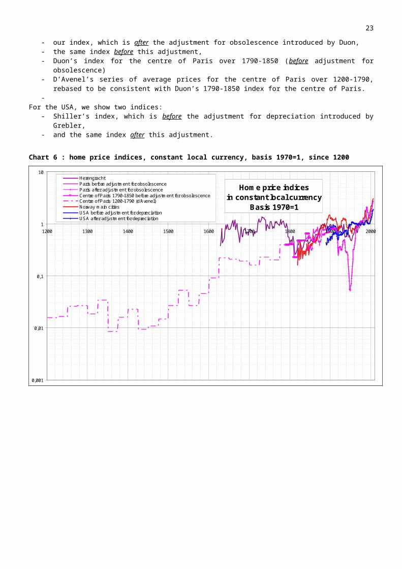
Chart 11 : Paris and US home price indices, constant local currency, basis 1970=1

Paris and USAHome price indices in constant local currency

Basis 1970=1

Exponential trend: US index after adjustmenty = 3E-08e0,0089x

R2 = 0,8588

Exponential trend: US index before adjustmenty = 0,0002e0,0044x

R2 = 0,5121

0,1

1

10

1840 1860 1880 1900 1920 1940 1960 1980 2000

Paris before adjustment for obsolescence

Paris after adjustment for obsolescence

USA before adjustment for depreciation

USA after adjustment for depreciation

Exponentiel (USA after adjustment fordepreciation)Exponentiel (USA before adjustment fordepreciation)

23

3.4.2. Impact of major events 3.4.2.1. WWI

The impact of WWI is much stronger on the Paris index than on the other indices, not only in constant currencies but also in nominal currencies (cf. charts 12).At first sight, this could be expected since Norway and the Netherlands stayed neutral, and the USA joined the war only in its final stages. Nevertheless, a closer analysis would be necessary to interpret properly this phenomenon. The strong impact of WWI on the Paris index was mostly caused by the implementation of rent controls in times of high inflation. During WWI proper47, inflation was not that much lower in Norway, and, though lower, was still considerable in the Netherlands and in the USA (cf. chart 13). It would be interesting to analyze whether similar rent controls were implemented in the Netherlands, Norway and the USA, and whether other factors (for instance, capital flight to supposed Dutch safety from various European countries during the war, or from Germany after the war?) also intervened.

Charts 12 : impact of WWI, nominal currencies and constant currencies

Impact of WWI: home price indices, basis 1914=1nominal currencies

0

0,5

1

1,5

2

2,5

1914 1916 1918 1920 1922 1924 1926

HerengrachtParisNorway main citiesUSA (22 cities) before adjustment for depreciationUSA (22 cities) after adjustment for depreciation

Impact of WWI: home price indices, basis 1914=1constant currencies

0

0,2

0,4

0,6

0,8

1

1,2

1,4

1914 1916 1918 1920 1922 1924 1926

Herengracht

ParisNorway main cities

USA (22 cities) before adjustment for depreciationUSA (22 cities) after adjustment for depreciation

Chart 13 : impact of WWI, consumer price indices

Impact of WWI: consumer price indices, basis 1914=1

0

1

2

3

4

5

6

7

1914 1916 1918 1920 1922 1924 1926 1928 1930

Netherlands

France

Norway

USA

47 The big difference between France and the three other countries considered here is that in the 1920’s the CPI kept increasing sharply in France, whereas it decreased or remained steady in the three other countries.

24

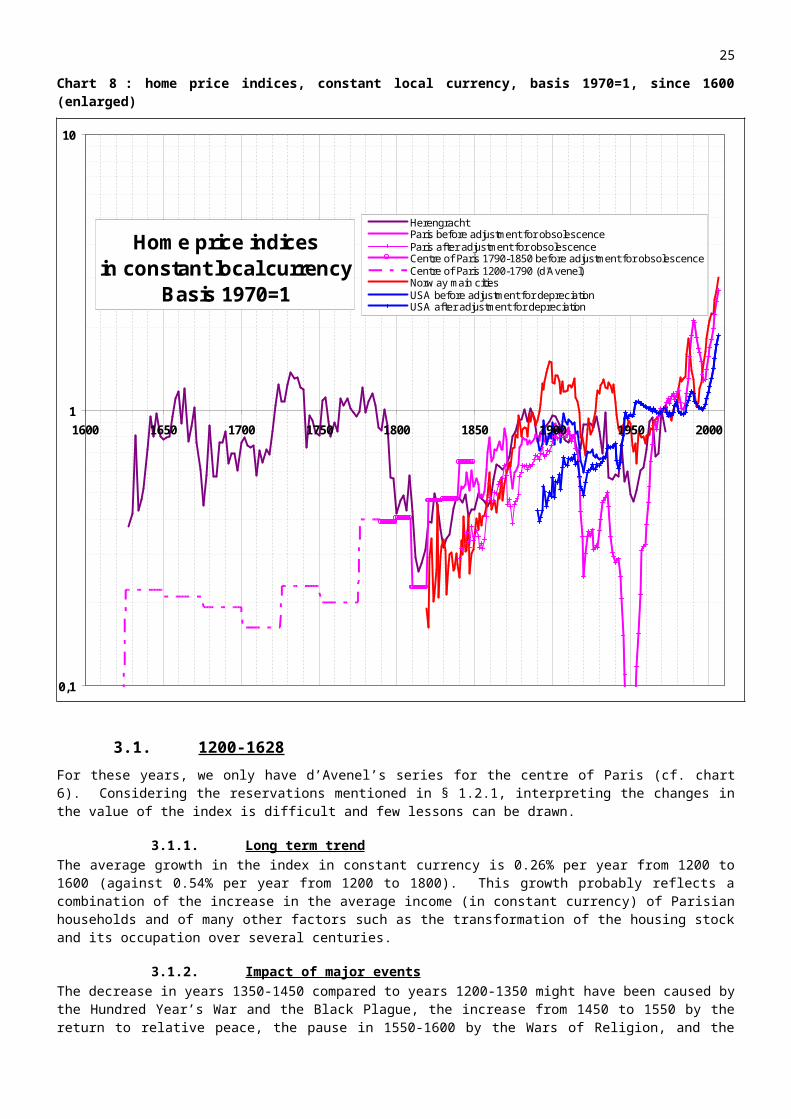
3.4.2.2. The 1929 crisisIn the early 1930’s, the Paris index increased significantly (cf. charts 14). Authors of that time explain this phenomenon partly by a partial relaxation of rent controls in the late 1920’s, but mostly by investors’ flight to the supposed safety of housing investment after the 1929 stock market crash reminded them of stock volatility. This steep price rise was followed by an equivalent fall in constant currency from 1935 to 1938.The three other indices do not show a similar pattern. Maybe this stems from the fact that the Paris index applies (for that period) to a pure investors’ buy-to-let market, whereas the three other indices apply to markets totally (in the case of the USA) or partially (in the cases of the Herengracht and Norway main cities) owner-occupiers’ markets. Maybe it stems from the differences in the timing and the depth of the economic crisis in the various countries. Maybe it stems from other causes, to be found.

Charts 14 : impact of the 1929 crisis, nominal currencies and constant currencies

Impact of the 1929 crisis: home price indices, basis 1928=1nominal currencies

0

0,2

0,4

0,6

0,8

1

1,2

1,4

1,6

1,8

1928 1929 1930 1931 1932 1933 1934 1935 1936 1937 1938

HerengrachtParisNorway main citiesUSA (22 then 5 cities) before adjustment for depreciationUSA (22 then 5 cities) after adjustment for depreciation

Impact of the 1929 crisis: home price indices, basis 1928=1constant currencies

0

0,2

0,4

0,6

0,8

1

1,2

1,4

1,6

1,8

1928 1929 1930 1931 1932 1933 1934 1935 1936 1937 1938

Herengracht

ParisNorway main citiesUSA (22 then 5 cities) before adjustment for depreciationUSA (22 then 5 cities) after adjustment for depreciation

Chart 15 : impact of the 1929 crisis, consumer price indices

Impact of the 1929 crisis: consumer price indices, basis 1928=1

0

0,2

0,4

0,6

0,8

1

1,2

1,4

1928 1929 1930 1931 1932 1933 1934 1935 1936 1937 1938

Netherlands

France

Norway

USA

25

3.4.2.3. WWIIIn constant currencies (cf. charts 16), the impact of WWII on the Paris index is even stronger than that of WWI, its cause being again the implementation of rent controls in times of high inflation, the inflation caused by WWII being even higher than that caused by WWI (cf.chart 17). In nominal currencies, this is not true, but this is due only to the very high inflation caused by WWII in France.In constant currencies still, the impact of WWII is also much stronger on the Paris index than on the three other indices48. This looks natural in the case of the US index. It is less so in the cases of the Herengracht index and Norway main city index, since both the Netherlands and Norway were occupied by Germany like France. A comparative analysis of inflation, monetary conditions, rent regulations, price dissimulation49, constraints imposed by the occupiers and other aspects in the Netherlands, France and Norway in that period might help explain this phenomenon.

Charts 16: impact of WWII, nominal currencies and constant currencies

Impact of WWII: home price indices, basis 1938=1nominal currencies

0

0,5

1

1,5

2

2,5

3

3,5

1938 1940 1942 1944 1946 1948 1950

Herengracht

Paris

Norway main cities

USA (5 cities)

Impact of WWII: home price indices, basis 1938=1constant currencies

0

0,2

0,4

0,6

0,8

1

1,2

1,4

1,6

1938 1940 1942 1944 1946 1948 1950

Herengracht

Paris

Norway main cities

USA (5 cities)

Chart 17 : impact of WWII, consumer price indices

Impact of WWII: consumer price indices, basis 1938=1

0

1

2

3

4

5

6

7

8

9

10

11

12

13

14

15

16

17

18

19

1938 1940 1942 1944 1946 1948 1950

Netherlands

France

Norway

USA

48 Same remark as in the previous paragraph for the comparison is nominal currencies.49 Cf. notes Error: Reference source not found and Error: Reference source not found.

26

3.5. Home price indices compared to income per household or proxies Since home prices and incomes per household are so highly correlated in space at a given time, and since their spatial hierarchies may have changed so widely in time, it may be interesting to compare the growth in home price indices to the growth in incomes per household.However, measuring income per household in a given area in the distant past is difficult.

- Since we are studying home prices, it is the very income per household (a household being constituted of the occupants of a dwelling) which is significant, rather than the income per person. Since the number of persons per household has decreased sharply in time (from 4.1 in 1861 to 2.4 in 2005 in France, from 4.9 in 1920 to 2.4 in 1990 in Norway, from 5.0 in 1890 to 2.7 in 2005 in the USA), the population is no substitute for the number of households. We found data about the number of households back to 1861 for France, back to 1920 in Norway, and back to 1850 in the USA.

- While the CPI may be relatively little differentiated spatially inside a given country (although this was less true in the distant past, due to poor transportation means), the income per household in a given area may drift significantly in time compared to all of the country (thus, the growth in the income per household in the 20th century may have been different, for instance, in Paris and in all of France).

- Data about income are rare in the distant past. The series we may find about workers’ salaries are a very poor substitute, since we don’t know the income of other inhabitants and the proportion of workers among the active population. For all of a given country, we have the series of households’ disposable income (for which we found data back to 1896 for France and 1921 for the USA, and much shorter series for Norway and the Netherlands). Assuming that households’ disposable income represented a more of less constant share of GDP (which is only partially true), we may try to content ourselves with GDP per household.

- We need data applicable to the areas covered by the four indices.o For the Herengracht, we have no data on households’ income (not to speak of “GDP” 50), and data

for all of the Netherlands cannot be a good substitute because of the small size of the neighbourhood.

o For Paris, the least bad substitute we have are data for all of France (GDP per household on all the period studied, and disposable income per household back to 1896), but over a century income and “GDP” may have grown at different paces in Paris and in all of France.

o For the main Norwegian cities, the least bad substitute we found are a series of GDP per household for all of Norway which doesn’t go farther back than 1920, and as is the case for Paris, income and “GDP” may have grown at different paces in the main Norwegian cities on one hand and in all of Norway in the other hand.

o For the USA, we have a series of GDP per household for all the period studied, but prior to 1953 the area covered by this index is much smaller (22 cities in the 1890-1934 period, 5 cities in the 1934-1953 period) than all of the USA, so here too there may be a bias.

Because of all these considerations and subject to these provisos, we have limited ourselves to showing the Paris index relative to French GDP per household, Norway main city index relative to Norwegian GDP per household and the US index relative to US GDP per household (chart 18).

50 We use brackets here because, as far as GDP is concerned, isolating a mere district (or even a city) from the rest of a country is very difficult and hardly significant.

27

Chart 18 : Paris, Norway main city and US home price indices relative to GDP per household, basis 1970=1

Paris, Norway main cities and USAHome price indices relative to GDP per household

Basis 1970=1

Exponential trend: US index after adjustmenty = 34550e-0,0053x

R2 = 0,5676

Exponential trend: US index before adjustmenty = 2E+08e-0,0097x

R2 = 0,7844

0,1

1

10

1840 1860 1880 1900 1920 1940 1960 1980 2000

Paris index before adjustment / French GDP per person

Paris index after adjustment / French GDP per household

Norway main city index / Norwegian GDP per household

US index before adjustment / US GDP per household

US index after adjustment / US GDP per household

Exponentiel (US index after adjustment / US GDP perhousehold)Exponentiel (US index before adjustment / US GDP perhousehold)

NB: in each case, the numerator and the denominator do not cover the same areas, which may bias their comparison.

The impact of Grebler’s adjustment for depreciation is clearly visible here too: the trend growth in the US index relative to GDP per household is -1% before adjustment and -0.5% after adjustment.

28

Since a home price index filters out many quality effects, and for other reasons (such as changes in the number of dwellings per household, linked to changes in the proportion of secondary homes, or a changing rent/price ratio), its trend growth is different from that of the housing expense mentioned in the National accounts, as chart 19 and chart 20 show. Thus, for instance, if the home price index grows like the average income per household, that does not mean that the average price of the homes purchased by households is constant with respect to the average income per households, nor that the weight of housing inside households’ income is constant.

Chart 19 : home price indices relative to disposable income per household, France, USA and UKHome price indices relative to disposable income per household

Comparison France - USA - UKBasis 2000=1

0

0,5

1

1,5

1950 1960 1970 1980 1990 2000 2010

France USA UK

Chart 20 : housing expense as a % of households’ disposable income, France, USA and UKHousing expense as a % of households'disposable income

Comparison France - USA - UK

0%

5%

10%

15%

20%

25%

1920 1930 1940 1950 1960 1970 1980 1990 2000 2010

FranceUSAUK

4. Conclusion This short analysis raises rather more questions than it brings answers.

Except on their most recent parts (the latest decades at best), the four indices compared here either don’t filter out the combination of aging and physical improvements or (in the case of Duon’s and Grebler’s indices) do it by a mere global adjustment. Thus, these indices cannot be called ‘constant quality’ indices (except again partly for Duon’s and Grebler’s indices when they are considered after adjustment).In addition, while the urban status and relative social status of the areas covered impact the value of the indices, they changed in ways which are probably very different depending on the area considered, and which cannot be measured accurately in the distant past.A first consequence is that one should refrain from extrapolating an index for a small area into an index for a whole country, for instance by generalizing the Herengracht index into a Netherlands index, the Paris index into an index for France, etc.A second consequence is that the long term trend of these indices should be interpreted with caution, and that it is quite difficult to infer from them “the long term trend growth of home price indices”.However, these considerations should not hide the fact that, in the long term, the yearly average growth in the four home price indices (not to be mistaken for average home prices) studied here has not been very different from that of the CPI, or in some cases the income per household (where this aggregate can be approximated), thus much lower than the growth rates experienced in most countries for the past few years.

In addition, secular indices are particularly interesting in that their ups and downs show how military, political, regulatory or economic events have impacted home prices in the course of history. Their recent availability has opened new, little explored, fields to research.

29

Appendix: data and sources

To open an Excel file containing the data, double click here:

A. Home price indices

A1) Herengracht index- Piet M.A. Eichholtz, A Long Run House Price Index: The Herengracht Index, 1629-1973, University of

Limburg, Maastricht and University of Amsterdam, Amsterdam, August 1996.

A2) Paris index- Distant past

o Georges d’Avenel, “Histoire économique de la propriété, des salaries, des denrées et de tous les prix en général depuis l’an 1200 jusqu’en l’an 1800” (“Economic History of Property, Salaries, Foodstuff, and All Prices in General from Year 1200 to Year 1800”), Imprimerie Nationale and Ernest Leroux, Paris, 1894-1912,

o Gaston Duon, “Évolution de la valeur vénale des immeubles parisiens” (« Evolution of the transaction price of Parisian buildings »), Journal de la Société de Statistique de Paris, October 1943, pages 169-192,

o Gaston Duon, « Évolution de la valeur vénale des immeubles à Paris de 1840 à 1939 » (« Evolution of the transaction price of buildings in Paris from 1840 to 1930 »), Bulletin statistique de la France, December 1943, pages 375-378,

o Gaston Duon, « Documents sur le problème du logement » (« Documents on the problem of housing »), Études Économiques, 1946, n°1, pages 1-165,

o Jacques Friggit, « Reconstitution des prix immobiliers passés à partir des bases de données notariales et de la série de Gaston Duon, note méthodologique » (« reconstitution of past property prices based on Notaries’ databases and Gaston Duon’s series »), working paper, unpublished, January 2002, 49 pages,

o Jacques Friggit, “L’évolution sur longue période du prix des logements”, Note de Synthèse du SES, March-April 2001, http://www.statistiques.equipement.gouv.fr/IMG/pdf/NS134-1-6_cle0236f4.pdf, 6 pages.

- Recent past: Notaires-INSEE indexo INSEE Méthodes n° 111 ,o Christian Gouriéroux & Anne Laferrère, « Managing Hedonic Housing Price Indices : the French

Experience », OECD-IMF Workshop on Real Estate Price Indexes, Paris, Nov. 2006, http://www.oecd.org/dataoecd/2/24/37583497.pdf.

o Anne Laferrère, “Who is afraid of hedonics? Lessons from the French Experience of Housing Price Indexes”, INSEE and CREST, soon on http://www.crest.fr/pageperso/anne.laferrere/anne.laferrere.htm.

A3) Norway main city index- Distant past:

o Øyvind Eitrheim and Solveig K. Erlandsen, House price indices for Norway 1819–2003, chapter 9 of Norges Bank Occasional Papers No 35 "Historical Monetary Statistics for Norway 1819-2003", June 2004: http://www.norges-bank.no/Pages/Article____42943.aspx,

o Øyvind Eitrheim and Solveig K. Erlandsen, House prices in Norway 1819–1989, Working Paper, Research Department, Norges Bank, November 11, 2004.

- Recent past: Norwegian Association of Real Estate Agents:o www.nef.no , NEF/EFF/FINN.no/ECON

A4) US index- Distant past:

o Grebler, Blank and Winnick, “Capital Formation in Residential Real Estate: Trends and Prospects”, (a study of the National Bureau of Economic Research published by Princeton University Press, Princeton, 1956),

o Robert J. Shiller, Irrational Exuberance, Second Edition, Currency Doubleday, 2005,o OFHEO index: http://www.ofheo.gov/HPI.aspx.

- Recent past: S&P/Case-Shiller National indexo http://www.macromarkets.com/csi_housing/documents/tech_discussion.pdf o http://www2.standardandpoors.com/portal/site/sp/en/us/page.topic/indices_csmahp/2,3,4,0,0,0,0,0,0,0,0,0,0,0,0,0.html .

B. Other data

30

B1) Consumer price indices NetherlandsWe used directly Eichholtz’s constant currency home price index, so implicitly we used his CPI, the sources of which are mentioned in (Eichholtz, 1996). The CPI mentioned in the Excel data file downloadable at the beginning of the present appendix is recalculated as the quotient of Eichholtz’s nominal and real indices.

France 1200-1790: in order to deflate our home price index (which over this period is derived from

d’Avenel’s house price series) by a deflator consistent with it, we use d’Avenel’s index of the purchasing power of silver (his nominal home price index being expressed de facto in grams of silver)51.

1790-1798 : average price of cereals (wheat, rye, barley, oat) as per Villa (CEPII) : http://www.cepii.fr/francgraph/bdd/villa/mode.htm.

1798-1820: «Essai sur les mouvements des revenus et l’activité économique en France de 1789 à 1820», A. Chabert, Librairie de Médicis, 1949.

1820-1913: Lévy-Leboyer M. et Bourguignon F., «L’Économie Française au XIXème siècle, analyse macroéconomique», M. Lévy-Leboyer et F. Bourguignon, Économica, 1985.

1913-2005: INSEE.

NorwayNorges Bank: http://www.norges-bank.no/Pages/Article____42931.aspx.

USA Before 1913: Historical Statistics of the United States (Bicentennial Edition, 1975). From 1913: US Bureau of Labor.

B2) GDP France

1815-1938: Toutain J.-C., «Le produit intérieur brut de la France de 1789 à 1982», Cahiers de l’ISMEA n°15, 1987 (missing years interpolated).

1938-2005: INSEE (missing years interpolated).

NorwayNorges Bank: http://www.norges-bank.no/Pages/Article____42937.aspx.

USA 1802- 1929: Historical Statistics of the United States (Bicentennial Edition, 1975). 1929-2005: Stats-USA.

B3) Number of households France

1840 to 1861: derived from the population series, assuming a constant number of persons per household (this may have led to overestimate the number of households in 1840, since household size probably decreased during that period).

From 1861: after INSEE (missing years interpolated, overseas department number of households extrapolated for most years).

NorwayStatistics Norway (www.ssb.no) (missing years interpolated).

USAUS Census Bureau (missing years interpolated).

51 In previous versions of this paper, we had used other sources for the 17 th and 18th century: estimates derived from “L’économie de l’Ancien Régime” (Jean-Yves Grenier, Albin Michel, 1996) for the 17 th century and Villa (CEPII)’s average price of cereals for the 18 th century. We don’t know of any undisputable consumer price index for France or Paris over this period of time. The impact of this change on the results in constant currency is secondary, and anyway for the 17th and 18th centuries the index in nominal currency is itself subject to the reservations mentioned in 1.2.1.

31

B4) Housing expenses and households’disposable income France, USA and UKNational accounts, per governments’ websites.

32