comparing cropping system productivity between fixed rotations

University of Nebraska - LincolnDigitalCommons@University of Nebraska - LincolnTheses, Dissertations, and Student Research inAgronomy and Horticulture Agronomy and Horticulture Department

Fall 12-2010

COMPARING CROPPING SYSTEMPRODUCTIVITY BETWEEN FIXEDROTATIONS AND A FLEXIBLE FALLOWSYSTEM USING MODELING ANDHISTORICAL WEATHER DATA IN THESEMI-ARID CENTRAL GREAT PLAINSJuan Jose Miceli-Garcia

Follow this and additional works at: http://digitalcommons.unl.edu/agronhortdiss

Part of the Plant Sciences Commons

This Article is brought to you for free and open access by the Agronomy and Horticulture Department at DigitalCommons@University of Nebraska -Lincoln. It has been accepted for inclusion in Theses, Dissertations, and Student Research in Agronomy and Horticulture by an authorizedadministrator of DigitalCommons@University of Nebraska - Lincoln.

Miceli-Garcia, Juan Jose, "COMPARING CROPPING SYSTEM PRODUCTIVITY BETWEEN FIXED ROTATIONS AND AFLEXIBLE FALLOW SYSTEM USING MODELING AND HISTORICAL WEATHER DATA IN THE SEMI-ARID CENTRALGREAT PLAINS" (2010). Theses, Dissertations, and Student Research in Agronomy and Horticulture. 38.http://digitalcommons.unl.edu/agronhortdiss/38

http://digitalcommons.unl.edu?utm_source=digitalcommons.unl.edu%2Fagronhortdiss%2F38&utm_medium=PDF&utm_campaign=PDFCoverPages

http://digitalcommons.unl.edu/agronhortdiss?utm_source=digitalcommons.unl.edu%2Fagronhortdiss%2F38&utm_medium=PDF&utm_campaign=PDFCoverPages


http://digitalcommons.unl.edu/ag_agron?utm_source=digitalcommons.unl.edu%2Fagronhortdiss%2F38&utm_medium=PDF&utm_campaign=PDFCoverPages


http://network.bepress.com/hgg/discipline/102?utm_source=digitalcommons.unl.edu%2Fagronhortdiss%2F38&utm_medium=PDF&utm_campaign=PDFCoverPages

http://digitalcommons.unl.edu/agronhortdiss/38?utm_source=digitalcommons.unl.edu%2Fagronhortdiss%2F38&utm_medium=PDF&utm_campaign=PDFCoverPages

COMPARING CROPPING SYSTEM PRODUCTIVITY BETWEEN FIXED

ROTATIONS AND A FLEXIBLE FALLOW SYSTEM USING MODELING AND

HISTORICAL WEATHER DATA IN THE SEMI-ARID CENTRAL GREAT PLAINS

by

Juan J. Miceli-Garcia

A THESIS

Presented to the faculty of

The Graduate College of the University of Nebraska

In Partial Fulfillment of Requirements

For the Degree of Master of Science

Major: Agronomy

Under the Supervision of Professors Drew J. Lyon and Timothy J. Arkebauer

Lincoln, Nebraska

December, 2011

COMPARING CROPPING SYSTEM PRODUCTIVITY BETWEEN FIXED

ROTATIONS AND A FLEXIBLE FALLOW SYSTEM USING MODELING AND

HISTORICAL WEATHER DATA IN THE SEMI-ARID CENTRAL GREAT PLAINS

Juan J. Miceli-Garcia, M.S.

University of Nebraska, 2011

Advisers: Drew J. Lyon and Timothy J. Arkebauer.

In the Central Great Plains, the predominant crop rotation is winter wheat

(Triticum aestivum L.)-fallow. Producers are looking to add diversity and intensity to

their cropping systems by adding summer crops, however, the elimination of summer

fallow may increase crop production risk. The objective of this study was to use crop

simulation modeling to compare the productivity of two fixed rotations [winter wheat-

corn (Zea mays L.)-fallow and winter wheat-corn-spring triticale (X Triticosecale

Wittmack)] with simulated flexible fallow rotations. The flexible fallow rotations made

the decision to plant triticale or use summer fallow prior to winter wheat seeding based

on available soil water in spring. Data from three years of field studies at two sites,

Sidney, NE and Akron, CO, were used to calibrate and test the model, AquaCrop, for the

crop simulation. Twenty-three years of historical weather data from each of the two

locations were used to simulate crop production for each rotation. Average income was

improved by replacing summer fallow with triticale (from 120 to 160 US $ ha-1

for Akron

and from 126 to 199 US $ ha-1

for Sidney), but income variability (standard deviation)

also increased (from 73 to 84 US $ ha-1

for Akron and from 93 to 115 US $ ha-1

for

Sidney). Risk-averse growers are likely to always use fallow in their crop rotations prior

to planting winter wheat, while non-risk-averse growers will likely eliminate fallow and

substitute triticale or a similar early-planted spring forage. Flexible fallow rotations

seldom improved profits compared to always using fallow without also increasing

income variability. The exception was Sidney using the 400 mm soil water threshold,

which lowered income variability compared to always fallowing (from 93 to 91 US $ ha-

1) and increased average income (from 126 to 142 US $ ha

-1). However, the economic

benefits of flexible fallow compared to the two fixed cropping systems were minimal.

iv

Acknowledgments

First of all I would like to thank God for all the blessings that He has given to me

and to my family. None of this would have been possible without Him.

I would like to acknowledge the advice and guidance of the members of my

graduate committee; Drew J. Lyon, David C. Nielsen, and Timothy J. Arkebauer for their

guidance, patience, effort and uncountable suggestions. The completion of my masters

program and graduation would not be possible without their help. I also want to thank

Osval Montesinos for his time as we developed the statistical analysis for this study, and

Paul Burgener for his help with the economic analysis.

I thank Vern Florke, Rob Higgins, Jamie Littleton-Sauer, and Albert Figueroa for

their help in the field work. I thank Marlene Busse for her patience answering all of my

questions regarding paper work. I also want to thank Sam and Mitch for their friendship

and advice. I wish to express special gratitude to Steve Mason, John Lindquist and

Charles Francis for always having a minute for me.

Thank you to the Anna H. Elliott Fund and the Nebraska Wheat Board for their

economic support for this project.

Thanks to my parents, Enrique and Yolanda and my brother and sister, Jose

Enrique and Lucia for their support and encouragement. Thanks for being the best family

that I possibly could have. Finally, but not least, I would like to thank Chelsea for her

love and unconditional support, not only during happy and sad moments, but also during

these long hours of work. I could not have done all this work without her love, support

and patience.

v

Table of Contents

Acknowledgments iv

Table of Contents v

List of Tables vi

List of Figures ix

INTRODUCTION 1

CHAPTER 1. Literature Review 3

1.1 Summer Fallow 3

1.2 Alternatives to Summer Fallow 7

1.3 Flexible Fallow 11

1.4 Crop Simulation Modeling 17

CHAPTER 2. Materials and Methods 28

CHAPTER 3. Results and Discussion 42

3.1 Aqua-Crop Calibration and Validation 42

3.2 Multi-year Simulation 43

CHAPTER 4. Conclusions 47

Tables 50

Figures 76

References 94

Appendix A 99

vi

List of Tables

Table 1 Planting and harvesting dates at Akron, CO. for corn, winter wheat and triticale.

................................................................................................................................50

Table 2 Planting and harvesting dates at Sidney, NE. for corn, winter wheat and triticale.

................................................................................................................................51

Table 3 Phenological stages at which various soil and crop measurements were taken

from each crop. .....................................................................................................52

Table 4 Crop parameters used in AquaCrop to simulate winter wheat. ...........................53

Table 5 Crop parameters used in AquaCrop to simulate triticale. ...................................54

Table 6 Crop parameters used in AquaCrop to simulate corn. ........................................55

Table 7 Historical prices for winter wheat, corn, and spring triticale. .............................56

Table 8 Production cost for winter wheat, corn, spring triticale and fallow. ...................57

Table 7 Statistics for the comparison between observed and simulated values for seed

yield, final biomass, and crop evapotranspiration (ET) for winter wheat and corn,

and final biomass and crop ET for triticale, for the calibration of AquaCrop for

Akron, CO. ............................................................................................................58

Table 8 Statistics for the comparison between observed and simulated values for seed

yield, final biomass, and crop evapotranspiration (ET) for winter wheat and corn,

and final biomass and crop ET for triticale, for the validation of AquaCrop for

Sidney, NE. ...........................................................................................................59

Table 9 Simulated grain yields for winter wheat and corn, and forage yields for triticale,

in two fixed rotations [winter wheat-corn-triticale (WW-C-T) and winter wheat-

vii

corn-fallow (WW-C-F) ] and flexible fallow using three different soil water

thresholds at planting (350, 375, and 400 mm) to determine when to plant triticale

or use fallow at Akron, CO. using historical weather data from 1988 through

2010. ......................................................................................................................60

Table 10 Simulated grain yields for winter wheat and corn, and forage yields for triticale,

in two fixed rotations [winter wheat-corn-triticale (WW-C-T) and winter wheat-

corn-fallow (WW-C-F) ] and flexible fallow using three different soil water

thresholds at planting (350, 375, and 400 mm) to determine when to plant triticale

or use fallow at Sidney, NE using historical weather data from 1988 through

2010. .................................................................................................................... ..61

Table 11 Summary of simulated grain yield for winter wheat and corn and forage yield

for triticale for Akron, CO. ...................................................................................62

Table 12 Summary of simulated grain yield for winter wheat and corn and forage yield

for triticale for Sidney, NE. ...................................................................................63

Table 13 Statistical comparison of average winter wheat grain yield predicted for each

cropping system at Akron, CO. .............................................................................64

Table 14 Statistical comparison of average winter wheat grain yield predicted for each

cropping system at Sidney, NE. ............................................................................65

Table 15 Statistical comparison of average corn grain yield predicted for each cropping

system at Akron, CO. ............................................................................................66

Table 16 Statistical comparison of average corn grain yield predicted for each cropping

system at Sidney, NE. ...........................................................................................67

viii

Table 17 Statistical comparison of average triticale biomass yield predicted for each

cropping system at Akron, CO. .............................................................................68

Table 18 Statistical comparison of average spring triticale biomass yield predicted for

each cropping system at Sidney, NE. ....................................................................69

Table 19 Economic returns for simulated grain yields for winter wheat and corn, and

forage yields for triticale, in two fixed rotations [winter wheat-corn-triticale

(WW-C-T) and winter wheat-corn-fallow (WW-C-F)] and flexible fallow using

three different soil water thresholds at planting (350, 375, 400 mm) to determine

when to plant triticale or use fallow at Akron, CO. using historical weather data

from 1988 through 2010. ......................................................................................70

Table 20 Economic return for simulated grain yields for winter wheat and corn, and

forage yields for triticale, in two fixed rotations [winter wheat-corn-triticale

(WW-C-T) and winter wheat-corn-fallow (WW-C-F)] and flexible fallow using

three different soil water thresholds at planting (350, 375, 400 mm) to determine

when to plant triticale or use fallow at Sidney, NE using historical weather data

from 1988 through 2010........................................................................................71

Table 21 Summary of economic returns for Akron, CO. .................................................72

Table 22 Summary of economic returns for Sidney, NE. ................................................73

Table 23 Statistical comparisons of average differences in economic returns between

cropping systems at Akron, CO. ...........................................................................74

Table 24 Statistical comparisons of average differences in economic returns between

cropping systems at Sidney, NE. ..........................................................................75

ix

List of Figures

Figure 1 Simulated vs. observed yield values for corn at Akron, CO…………………..76

Figure 2 Simulated vs. observed biomass values for corn at Akron, CO.........................77

Figure 3 Simulated vs. observed ET values for corn at Akron, CO…………………….78

Figure 4 Simulated vs. observed biomass values for triticale at Akron, CO………....…79

Figure 5 Simulated vs. observed ET values for triticale at Akron, CO……………...….80

Figure 6 Simulated vs. observed yield values for winter wheat at Akron, CO……..…...81

Figure 7 Simulated vs. observed biomass values for winter wheat at Akron, CO………82

Figure 8 Simulated vs. observed ET values for winter wheat at Akron, CO……………83

Figure 9 Simulated vs. observed yield values for corn at Sidney, NE…………………..84

Figure 10 Simulated vs. observed biomass values for corn at Sidney, NE……………...85

Figure 11 Simulated vs. observed ET values for corn at Sidney, NE…………………...86

Figure 12 Simulated vs. observed biomass values for triticale at Sidney, NE………….87

Figure 13 Simulated vs. observed ET values for triticale at Sidney, NE………………..88

Figure 14 Simulated vs. observed yield values for winter wheat at Sidney, NE………..89

Figure 15 Simulated vs. observed biomass values for winter wheat at Sidney, NE…….90

Figure 16 Simulated vs. observed ET values for winter wheat at Sidney, NE………….91

Figure 17 Box plots of income using different cropping systems at Akron, CO. ………92

Figure 18 Box plots of income using different cropping systems at Sidney, NE. ……...93

1

INTRODUCTION

In the western portion of the Central Great Plains, the predominant crop rotation

is winter wheat (Triticum aestivum L.)-fallow using mechanical tillage (Lyon et al., 1993;

Dhuyvetter et al., 1996). Summer fallow is an important, and sometimes indispensable,

component in the production of winter wheat due to the low amount of highly variable

precipitation in this region (450 mm or less annually) (Lyon et al., 1993). The primary

objective of summer fallow is the storage of water in the soil for use by the next wheat

crop (Nielsen et al., 2011). This is accomplished, in part, by controlling the growth of

weeds (Tanaka et al., 2010). However, there are years when precipitation is great enough

to allow summer fallow to be replaced by a short-season spring-planted crop (a concept

that is referred to as “Flexible Fallow”).

In the semiarid portion of the Great Plains, mainly in the western portion,

continuous cropping systems are risky due to limited precipitation and high potential

evapotranspiration (ET) (Nielsen et al., 2005). The rain shadow caused by the Rocky

Mountains, where elevations exceed 4200 m, results in a decline in annual precipitation

from east to west in Nebraska (Lyon et al., 2003). Summer fallow is a common practice

used in regions where annual precipitation is less than 500 mm per year (Farahani et al.,

1998). In the Great Plains, 75% of annual precipitation is received during the warm

season (April through September). The amount of water stored in the soil during summer

fallow is low, and changes in the amount of water stored over the fallow period can be

negative (Farahani et al., 1998). The climatological conditions of the Central Great

Plains, where water is the most limiting resource for crop production, makes winter

2

wheat-fallow the most commonly used production system in order to stabilize the

production of winter wheat in this region (McGee et al., 1997; Smika, 1970; Farahani et

al., 1998; Lyon et al., 2004).

Unpredictable weather conditions such as variable precipitation, temperature

fluctuation, and hail make dryland farming in the Great Plains uncertain (Dhuyvetter et

al., 1996). In order to achieve success and sustainability in the dryland agriculture

systems of the Great Plains, a more efficient use of the erratic precipitation and stored

soil water is necessary (Saseendran et al., 2009; Nielsen et al., 2005).

3

CHAPTER 1. Literature Review

1.1 Summer Fallow

Fallow attempts to limit the growth of all plants during the non-crop season,

thereby increasing the amount of soil moisture stored (Lyon et al., 2004; Dhuyvetter et

al., 1996). The control of plant growth is accomplished by either cultivation or herbicide

application (Brown et al, 1983).

Summer fallow was first practiced in the Great Plains during the 19th century by

farmers as a way to improve yields in small grain production, reduce crop failure, and to

reduce labor (Farahani et al., 1998). The lack of crop selection and adverse weather

conditions in the Great Plains during 1912 to 1921, led to the wheat-fallow system

becoming the dominant agricultural system in this region (Tanaka et al., 2002, Tanaka et

al., 2010).

For winter wheat in the Great Plains, the fallow period is approximately 14

months (Farahani et al., 1998). The main objective of a fallow period is to increase the

total amount of stored soil water to then be used by the following crop (Moret et al.,

2006). Other benefits that can be achieved with fallow are the release of nutrients into the

soil through the mineralization of soil organic matter and weed control (Aase et al., 2000;

Johnson et al., 1982). Fallow allows for stability in both production and yield, and a

better seasonal distribution of work (Johnson et al., 1982).

Even though the objective of fallow is to stabilize production for the next crop by

primarily helping to store water in the soil, it has been found that soil water is stored

4

inefficiently in fallow systems, frequently averaging less than 25% precipitation storage

efficiency (Lyon et al., 2004; McGee et al., 1997; Nielsen and Vigil, 2010).

Farahani et al. (1998) divided fallow in the winter wheat-fallow system into three

periods: early period (from July after wheat harvest to mid-September), overwinter period

(fall to early May), and late period (from spring to mid-September at wheat seeding).

Further, they mention that the winter period is the most efficient at storing soil water,

having the lowest amount of evaporation and greatest water storage efficiency, even

though this period has the lowest precipitation rate. On the other hand, the late period,

also known as summer fallow, is the most inefficient at storing soil water, even though it

is the period that receives the greatest amount of precipitation (Farahani et al., 1998). In

the non-crop periods of the wheat-fallow system, most of the precipitation is lost by

evaporation, deep percolation, and runoff (Black et al., 1981).

In Australian dryland wheat production, Angus et al. (2001) reported that little

water is stored during the fallow period. Most of the precipitation received during the

fallow period is lost due to soil evaporation, weed use, volunteer plants, runoff, deep

seepage, and snow blow-off (Farahani et al., 1998). Nielsen et al. (2005) mentions that

when tillage is used during summer fallow, the degradation of crop residues make the soil

more vulnerable to wind erosion and the reduction in the size of the crop residue particles

make them less effective for evaporation reduction. Additionally, the formation of a soil

crust by the impact of rain drops on unprotected soil reduces the water infiltration

capability of the soil (Nielsen et al., 2005). Crop residues allow for the protection of soil

against rain drop impact, the reduction of evaporation, the enhanced retention of

5

infiltrated water, and the maximum rates of water infiltration are achieved (Peterson et

al., 1993).

Under intense tillage, the water storage efficiency of fallow is as low as 10%

(Farahani et al., 1998). Moret et al. (2006) comments that in Spain, moldboard and chisel

plowing have had an adverse effect on soil water conservation when fallow was applied

for the first time during a very wet autumn. Deeper tillage mixed weed seed into deeper

soil layers and reduced the effectiveness of herbicides compared to herbicide use with

shallow tillage (Black et al., 1981). Research by Black et al. (1981) found that the control

of weeds, such as wild oat (Avena fatua L.), is better with herbicides when the land has

not been tilled to a depth of more than 7.5 cm. Reduction in tillage increases residue

cover that allows for a reduction in soil erosion and increase in production. Reduced and

no-till farming practices have improved the efficiency of precipitation capture and

storage, allowing a reduction in the use of fallow and more intensive cropping systems

(Lyon et al., 1995). Nielsen et al. (2010) found that the precipitation storage efficiency in

the wheat-fallow system is higher with no-till (35%) than when conventional tillage is

used (20%). Precipitation storage efficiency can be increased up to 20 to 30% when

farmers use no-till and residue management techniques commonly used today. The

increase in water storage efficiency is due to the reduction in the number of times that

moisture is brought to the soil surface as tillage is eliminated (Farahani et al., 1998;

Nielsen et al., 2005). Note that even with the best technology available today, the water

storage efficiency of fallow remains low, i.e., less than 45%.

6

Soil erosion is an important aspect that needs to be taken into consideration by

producers during the evaluation of cropping systems (Dhuyvetter et al., 1996, Young et

al., 1986). Wind and water erosion are the two most obvious disadvantages of summer

fallow (Burt et al., 1989). The use of tillage during fallow exposes soil to degradative

forces such as C removal by erosion, the acceleration of C oxidation, and less C being

deposited in the soil surface in comparison with conditions found for native prairie

(Peterson et al., 1998). Soil erosion and saline seeps are two sources of pollution of air

and water that can result from fallow and affect society (Johnson et al., 1982). Reduced

soil productivity and profitability of the farm are other problems related to the use of

summer fallow in dryland cropping systems (Lyon et al., 2004).

Fallow may represent an economic disadvantage for growers, in part, because

mechanical tillage represents a big cost, and because the area required for an annual

cropping system is doubled (Lyon et al., 2007, Tanaka et al., 2010). In addition, anytime

the land is not producing there is an opportunity cost, which is higher in years with high

crop prices (Johnson et al., 1982). In an extended literature review made by Dhuyvetter et

al. (1996), it was found that even with the inclusion of government program payments for

wheat, more intensive cropping systems were more profitable than the traditional wheat-

fallow cropping system in the Central Great Plains.

Other important effects such as the reduction in soil aggregates, destruction of

residues, and N mineralization have been reported as disadvantages of tillage during the

fallow period (Peterson et al., 1993). The uses of monoculture systems such as wheat-

fallow promote not only soil degradation and the reduction in the profitability of the

7

system, but also disease, weed, and insect problems (Daugovish et al., 1999; Nielsen et

al., 2009).

The decision to fallow land is made by individual farmers, making the total

amount of fallowed land greater than the optimal amount for society, consequently,

benefiting growers solely in the short term (Johnson et al., 1982). Conditions such as the

Dust Bowl in the 1930s were created, in part, by frequent use of tillage operations in the

control of weeds in fallow systems (Farahani et al., 1998).

The frequent use of summer fallow in the Central Great Plains can be hazardous

for crop production systems, creating ecological, economic, and social problems. Because

of this, other alternatives need to be explored that reduce the need for the use of summer

fallow.

1.2 Alternatives to Summer Fallow

The agricultural systems of the Central Great Plains are very reliant on summer

fallow (McGee et al., 1997). However, because of the environmental and economical

implications of the winter wheat-fallow rotation, a different approach that allows for a

more efficient use of water is needed.

In order to generate alternatives to the use of summer fallow, the improvement of

existing techniques and development of new ones to increase soil water retention and

conservation during the non-crop period are necessary (Black et al., 1981). This

improvement or new development needs to include crop residue management techniques

(such as reduced till and no-till), reduction of the length and/or frequency of the fallow

period, and adequate crop selection (Nielsen et al., 2005).

8

Farmers in the dryland cropping regions are looking for options other than the

traditional monoculture systems such as wheat-fallow (Nielsen et al., 2009; Zentner et al.,

2009). The use of herbicides for weed control during fallow helps to conserve soil water

and allows growers to produce crops more intensively (Lyon et al., 1983). Reduction in

tillage due to chemical weed control has increased wheat yields by 37% in wheat-fallow

systems compared with systems involving tillage (Nielsen et al., 2002). These

enhancements have increased economic returns and improved environmental

sustainability (Zentner et al., 2005).

Dhuyvetter et al. (1996) suggested that the use of a more intensive cropping

system than wheat-fallow, in combination with less tillage, can be an option for many

parts of the Great Plains currently using the wheat-fallow production system. The water

stored in the spring of the fallow year by using no-till, can be as much or more than the

water stored if fallow is continued until wheat planting in the fall (Peterson et al., 1996).

The use of more intense cropping systems with no-till will use the water stored in the

soil, and increase productivity per unit of water received and replace summer fallow in

many environments (Peterson et al., 1993; Tanaka et al., 2010). The increase in intensity

in the system allows a crop to be produced annually on 67 to 100% of the tillable land

(Dhuyvetter et al., 1996).

Loss of soil organic C and N is promoted by fallow (Peterson et al., 1993). More

intensive cropping systems have higher grain and crop residue production, less soil

disturbance that results in increased C content of the soil, and reduced C losses (Peterson

et al., 1998). The increase in residue C, in addition to no soil disturbance in a no-till

9

environment, promotes aggregate stability, which will positively impact the physical and

chemical properties of the soil (Tanaka et al., 2010).

Crop intensification in the Great Plains increases precipitation use efficiency on a

biomass-produced and price-received basis (Nielsen et al., 2005). Peterson et al. (1993)

found that increasing intensification of cropping systems will be an environmentally and

economically sustainable practice even in more water stressed environments.

Producers have shown some resistance to changing traditional production

systems. Some of the reasons for the slow change are: returns will not cover added costs

of machinery, herbicides and fertilizer; the relatively low labor required in wheat-fallow

systems; the increase in financial and production risks; and the ability to comply with

government programs (Dhuyvetter et al., 1996).

The reduction of summer fallow length and/or frequency will diminish soil

erosion, improve the efficiency of water use, and increase the long-term viability of

dryland farming in the Great Plains (Lyon et al., 2004; Tanaka et al., 2002). A reduction

of summer fallow by crop intensification, e.g., from one crop in 2-yr to two crops in 3-yr,

increases precipitation use efficiency (Nielsen et al., 2005). McGee et al. (1997) found

that a 3-yr rotation with a fallow period of 11 months was as efficient at storing water as

a fallow period of 14 months (McGee et al., 1997). The increase in crop intensification to

two crops in three years had little effect on the water available at wheat planting and on

wheat yield (Nielsen et al., 2002).

With the implementation of crop intensification, higher production of grain per

unit of water is achieved (Peterson et al., 1998). The key point of water use efficiency in

10

crop intensification is the replacement of water evaporation from the soil surface by crop

transpiration (Farahani et al., 1998, Tanaka et al., 2010). The use of perennial grass that

resembles the native prairie vegetation provides the highest water use and the least

erosive soil condition (Peterson et al., 1993). However, this last option will not allow for

the production of a wheat crop. More intensive systems such as wheat-sorghum-fallow

showed less financial risk than wheat-fallow (Dhuyvetter et al., 1996). Daugovish et al.

(1999) found that 3-yr rotation systems provide at least the same economic return as

wheat-fallow production, and in addition, provided excellent control of winter annual

grass weeds. The longer a field stays in a 3-yr rotation with a summer crop, the greater

the reduction in winter annual grass weeds (Daugovish et al., 1999). No significant

differences were found between wheat yields from wheat-fallow (no till), wheat-corn-

fallow, and wheat-millet-fallow systems (Nielsen et al., 2002).

The most efficient way to improve cropping system water use is to substitute a

summer crop for summer fallow (Farahani et al., 1998), and the frequency of summer

fallow can be reduced by reducing or eliminating tillage and increasing precipitation

storage efficiency between crops (Peterson et al., 1993). An early harvest, or short

duration spring-planted crop, used in transition from a full-season summer crop to winter

wheat minimizes the impact of not having summer fallow on the following winter wheat

(Lyon et al, 2004). Wheat following an early planted summer crop exhibited greater tiller

production, faster germination, and more growth compared to wheat following a late

planted summer crop (Lyon et al., 2007). The use of forage crops prior to winter wheat

seeding, due to the early date of harvest, allows more time for soil water storage than the

11

use of grain crops (Lyon et al., 2004). Dhuyvetter et al. (1996) analyzed the economics of

eight studies of dryland cropping systems in the Great Plains and found that in seven of

these studies the net return was greater in a more intensive crop rotation in combination

with practices of reduced-till or no-till following wheat harvest and prior to planting the

summer crop, than from the wheat-fallow rotation.

Spring triticale (X Triticosecale rimpaui Wittm.), dry pea (Pisum sativum L.),

foxtail millet (Setaria italica L. Beauv.), and proso millet (Panicum miliaceum L.) are

short-season crops that can be used in crop rotation to replace summer fallow

(Saseendran et al., 2009). Lyon et al. (2004) found that rotations that involved oat (Avena

sativa L.) + pea for forage or proso millet as summer fallow replacement crops were

economically competitive with summer fallow.

1.3 Flexible Fallow

Cropping decisions need to be based on the amount of soil water at planting and

expected precipitation during the growing season (Black et al., 1981). The practice of

having a continuous cropping system (no monoculture), where the selection of the crops

depends on the water available in the soil profile is defined as “opportunity cropping”

(Nielsen et al., 2005 ; Peterson et al., 1993). Lyon et al. (1995) defined it as a “flexible

cropping system”. A flexible cropping system involves planting a crop when the stored

soil water and the expected precipitation are considered sufficient for a successful crop.

In years where the water is not sufficient, fallow is implemented (Black et al., 1981).

Flexible cropping systems avoid the rigidity of fixed cropping. The implementation of a

12

flexible cropping system along with proper crop and soil management can reduce or

eliminate the necessity of summer fallow (Black et al., 1981).

In order to be successful in the development of a flexible cropping system, it is

necessary to take into consideration the relationship between initial soil water and

subsequent yield of the crop (Lyon et al., 1995, and Young et al., 1986). Zentner et al.

(2005) evaluated the use of an annual legume green manure crop as a summer fallow

substitute depending on the available soil water reserves. In this experiment, they found

that the “flex-crop” rotation had greater earnings than more traditional rotations, such as

those that include fallow. Lyon et al. (1995) analyzed the response of five spring-planted

crops to three different soil water levels at planting the year following winter wheat

harvest. The crops analyzed were corn, grain sorghum, pinto bean (Phaseolus vulgaris

L.), proso millet and sunflower (Helianthus annuus L.). They found that for pinto bean

and proso millet, soil water at planting appeared to be a good indicator of the success of

these short duration crops. However, for the long duration crops (corn, grain sorghum,

and sunflower), soil water at planting did not appear to be a good indicator of grain yield

(Lyon et al., 1995). This conclusion was verified by Nielsen et al. (2009) for dryland corn

in Colorado. Other points to take into consideration in the success of flexible cropping

are crop management and soil factors such as fertility and weed control (Black et al.,

1981).

Flexible cropping systems allow farmers a better use of environmental and/or

market conditions due to better adaptability from a bigger portfolio of crop options

(Hanson et al., 2007). Flexible cropping systems can control the risk of production and

13

soil loss, being in this way an option to respond to the challenges that agricultural

systems will be facing in the future due to uncertain conditions (Hanson et al., 2007,

Young et al., 1986).

The concept known as “flexible fallow” consists of the substitution of a short-

season, spring-planted crop for summer fallow when the soil water at planting is

sufficient, thus reducing soil degradation by summer fallow without significantly

compromising the next winter wheat crop (Felter et al., 2006). Flexible rotations that

allow the decision to fallow or not based on available soil water in spring represent a

more effective option than fixed rotation (Zentner et al., 2005). By fallowing in the driest

springs and planting a spring crop when the soil water at planting is sufficient, the farmer

has the opportunity to increase the sustainability of the system, obtain a higher income,

and reduce the riskiness of a fixed spring cropping system (Young et al., 1989).

In dryland crop production, the amount of soil moisture at seeding is usually a

limiting factor (Young et al., 1989). Nielsen et al. (1999, 2002 and 2009) conducted

many experiments to evaluate the relationship between soil water at planting and yield of

different crops used to diversify the wheat-fallow system. Wheat and millet yield, planted

after sunflower, declined as soil water at planting declined at Akron, CO (Nielsen et al.,

1999). In 2002, Nielsen et al. found a linear relationship between wheat grain yield and

soil water at planting. In the same study, they found that the intensification of the

traditional wheat-fallow system under no-till by the addition of a crop (corn or millet)

between wheat and fallow reduced the fallow period and did not significantly affect the

yield of the next wheat crop or the soil water available at wheat plating (Nielsen et al.,

14

2002). Nielsen et al. (2009) mention that corn can be used as a rotation crop in order to

diversify the traditional monoculture wheat-fallow system in the Central Great Plains.

The study showed that under dryland conditions, there is a positive relationship between

the soil water at planting and corn grain yield, with the slope of the relationship

increasing dramatically as precipitation during the flowering and grain filling stages

increased.

Zentner et al. (2005) compared the economic benefits of substituting an annual

legume green manure for summer fallow based on available soil water. The legume was

seeded and turned down before it reached full bloom to allow maximum N2 fixation, but

at the same time minimize soil water depletion. The conclusions of this study were that

flexible cropping systems usually ranked second in annual net returns, just behind

continuous wheat when using conservation tillage practices in order to enhance soil water

reserves, and under favorable growing conditions. The least profitable cropping systems

were fallow-wheat-wheat and annual legume green manure-wheat-wheat.

Good results were obtained by using annual legume green manure from

Indianhead black lentil (Lens culinaris Medikus) and chickling vetch (Lathyrus sativus

L.) cv. AC Greenfix as replacement crops for fallow when the soil water reserve in spring

was enough to avoid compromising the following wheat crop (Zentner et al., 2005).

The implementation of flexible fallow seems to have a better response when a

short duration summer annual crop is used (Lyon et al., 2007). In the western portion of

the Great Plains, forage crops had higher precipitation use efficiency on a biomass-

produced basis in comparison to oilseed crops or continuous small-grain production

15

(Nielsen et al., 2005). Short duration annual forage crops such as triticale and foxtail

millet use less water than grain crops because the length of the growing season is reduced

by harvesting prior to grain development, which is often the period of greatest water use

(Lyon et al., 2004; Lyon et al., 2007).

Saseendran et al. (2009) mentions that spring triticale and foxtail millet as forage

crops, and proso millet as a grain or forage crop, have the potential to substitute for

summer fallow in the winter wheat-fallow system.

Felter et al. (2006) used spring planted crops to evaluate substitutes for summer

fallow when soil water was sufficient at planting. They used four crops: spring triticale

for forage, dry pea for grain, proso millet for grain, and foxtail millet for forage. They

concluded that triticale, foxtail millet, and proso millet can be used as substitutes for

summer fallow in a flexible fallow cropping system based on available soil water at

planting. They found a linear relationship between dry matter accumulation and soil

water availability at planting time for triticale and foxtail millet. The two forage crops in

this study, spring triticale and foxtail millet, had an increase in harvested biomass for

each centimeter of water available at planting of 229 kg ha-1

and 339 kg ha-1

respectively

(Felter et al., 2006). They found that soil water at planting has a stronger relationship

with yield in years where seasonal precipitation is limited. The early harvest date of

triticale allows for more time to accumulate water in the soil prior to winter wheat

seeding compared to foxtail millet, which is planted and harvested later than spring

triticale (Lyon et al., 2007).

16

Producers and agricultural lenders need ways to assess the level of risk that the

increase in intensity of the traditional wheat-fallow rotation creates (Nielsen et al., 2002).

The study by Felter et al. (2006) suggests that soil water at planting can be used as an

indicator of yield potential for a short-season spring-planted crop used as a substitute for

summer fallow, particularly for crops grown for forage.

A short-season spring-planted forage crop such as triticale can be used as a

substitute for summer fallow in years where the amount of stored soil water at planting is

enough to produce sufficient triticale biomass without significantly reducing grain yield

of the following winter wheat crop (Felter et al., 2006; Lyon et al., 2007). Lyon et al.

(2007) found that the decision to plant or not plant a short-season crop as a summer

fallow replacement is more critical than the selection of what crop is planted. Since the

water available at planting for the short-season summer fallow replacement crop is

critical not only for the summer crop, but also for the following wheat crop, the

determination of the threshold soil water at which to plant the crop is a key point for the

success of the flexible fallow system (Lyon et al., 2007).

The use of summer fallow needs to be a judicious decision and not a habitual

practice (Black et al., 1981).The flexible fallow system can help growers increase crop

production during wetter years and minimize the risk of crop loss in dry years (Lyon et

al., 1995). In regions such as western Nebraska, where crop production is limited by lack

of precipitation, soil water at planting might be a good predictor for potential yield. The

development of a tool that helps growers to decide when to substitute a short-season

spring-planted crop for summer fallow might be useful (Felter et al., 2006).

17

1.4 Crop Simulation Modeling

In regions where the environmental conditions make production decisions

uncertain, models have been successfully used to analyze agronomic practices (Lyon et

al., 2003). In the Central Great Plains, long-term experiments to evaluate crop rotation

effects on water use and yield have been done since the 1990s (Saseendran et al., 2010).

However, there are not many long-term experiments that can be used to evaluate the

impact of no-till and altered crop rotations on the wheat-fallow system (Peterson et al.,

1993). Dryland cropping systems research in the Great Plains has to confront the

difficulty of conducting experiments over a long time period, with the demand of high

investment in many resources such as land and labor (Staggenborg et al., 2005). The

ability of conventional statistical techniques to extrapolate location-specific findings to

other regions and climates with heterogenic land conditions, such as the one presented in

the semiarid regions, is questionable (Saseendran et al., 2010).

The effect of summer fallow is well known in specific locations, but limited

information is available about extrapolating this information to locations with different

soil and climatic conditions (Peterson et al., 1993). With modeling, it is possible to see

the way that an agricultural crop will behave in other locations, climates, seasons, and

soils (Saseendran et al., 2009). The combination of long-term simulation with field

research data may give a good prediction of performance for new crops included in the

system, after only a couple of seasons of field data, avoiding the necessity of long-term

experiments (Staggenborg et al., 2005). This saves time and money in agricultural

research and accelerates the delivery of technologies to producers.

18

Field research results can be limited to the period of time in which they were

conducted, however, with crop modeling and long-term climate data, it is possible to

make an analysis that will allow for an adjustment of recommendations, avoiding the

time limitation of field research (Lyon et al., 2003; Staggenborg et al., 2005). Models are

needed to sensitize results obtained from long-term experiments in order to make

adequate management decisions in the Central Great Plains (Saseendran et al., 2010). The

combination of historical weather data and simulation modeling can be used to predict

system stability and the potential effect of future climatic changes (Peterson et al., 1993).

Modeling is a tool that can be used by producers to avoid the risks implied in the

adoption of new crops and practices (Staggenborg et al., 2005). In order to offer this tool

to producers, the development of the model for the crop selected is necessary, along with

its conscious calibration and testing of its performance under the climate of the region

(Saseendran et al., 2009).

Moret et al. (2006) mentions that even though there are many different crop

models, only a few of them have been applied to the study of soil water changes during

the fallow period.

Stochastic dynamic programming (DP) has been used to select dryland cropping

systems with high average annual returns, low variability, and reduced risk for water

percolation below the root zone (Burt et al., 1989). Young et al. (1986) used DP and

target prices for barley (Hordeum vulgare L.) to evaluate flexible cropping systems in

traditional wheat-fallow rotations. In this study, the authors were able to identify the

critical level of available soil moisture at planting for a flexible cropping strategy in a

19

wheat-fallow system using barley. They found that reduced soil erosion, improved

profitability, and reduced risk associated with continuous cropping were possible with the

use of DP and a flexible cropping approach in the traditional wheat-fallow system of the

region.

Stochastic dynamic programming can help to improve the economics of dryland

cropping systems, although the lack of data for different locations represents a problem

for this approach (Burt et al., 1989). The use of well calibrated and tested crop simulation

models can help to overcome this lack of information.

Another tool is the Crop Sequence Calculator, which is a relatively simple

program that gives information to the user about crop production, economics, diseases,

weeds, water use and soil properties, in order to evaluate different crop sequences

(USDA, 2011). However, the Crop Sequence Calculator does not predict crop yield

response to variable environmental conditions. Farmer interest in this relatively simple

program demonstrates the potential and necessity of more robust decision support tools in

order to increase the sustainability of the wheat-fallow cropping system (Tanaka et al.,

2010).

Root Zone Water Quality Model (RZWQM), Decision Support System for

Agrotechology Transfer (DSSAT), Cropping System Model (CSM), and Agricultural

Production System Simulator (APSIM) are some of the modeling programs reported in

the literature as being used to simulate the effects on yield and soil water use from

changes to the traditional cropping systems of the Central Great Plains.

20

RZWQM was developed by the Agricultural Research Service of the United

States Department of Agriculture. The model simulates the impact that alternative

management strategies have on plant growth, movement of water, nutrients, and agro-

chemicals within, over, and below the root zone (USDA, 2009).

DSSAT is a simulation package developed by the International Benchmark Sites

Network for Agrotechnology Transfer. DSSAT has been in use for over 15 years.

DSSAT allows the integration of soil, crop, phenotype, weather, and management in a

multi-spatial and multi-temporal simulation. DSSAT v4.0 includes 27 different crops and

the ability to analyze the environmental impact and economic risk of climate change, soil

carbon sequestration, climate variability, and nutrient and irrigation management

(ICASA, 2011).

RZWQM with DSSAT v4.0 crop growth modules (RZWQM2) was used by

Saseendran et al. (2009), who used data from two different Great Plains locations with

different plant available water levels and planted in different years, to successfully

simulate the response of summer crops used as a substitute for summer fallow in the

semiarid climate of the High Plains. The crops investigated were: spring triticale, proso

millet, and foxtail millet. For this experiment, the Cropping System Model (CSM)-

CERES-Wheat v4.0 module was adapted for the simulation of spring triticale growth

while the CSM-CERES-Sorghum module was adapted for proso millet and foxtail millet.

Modeling was used as an accurate tool to simulate the crop growth and development of

the three short-season crops as possible substitutes for summer fallow through multiple

years and different locations (Saseendran et al., 2009).

21

In 2010, Saseendran et al. evaluated the cropping system model RZWQM2 with

the DSSAT v4.0 in two traditional rotations in the Central Great Plains: wheat-fallow and

wheat-corn-fallow. The simulations were done from 1992 to 2008 and the calibration of

the model was made with data from the wheat-corn-millet rotation at Akron, CO from

1995 to 2008. The model was able to successfully simulate long-term sequential yield,

biomass production, and water and precipitation use efficiencies in crop rotations

involving wheat, millet, corn, and fallow in the Central Great Plains. Cropping systems

successfully simulated were: wheat-fallow, wheat-corn-fallow, and wheat-corn-millet. In

addition to these rotations, without further calibration, the model predicted accurately

enough the average yield of corn, millet, and wheat in the wheat-millet-fallow and wheat-

corn-millet-fallow rotations (Saseendran et al., 2010).

Staggenborg et al. (2005) used CERES-Wheat and CERES-Sorghum to simulate

wheat-fallow and wheat-sorghum-fallow systems in western Kansas. Wheat was better

simulated than sorghum. The error contained in the simulation of wheat, overestimated

by 10%, was higher than the one reported by other authors, suggesting that CERES-

Wheat does not perform as well under dryland conditions such as that of the Great Plains.

The authors mention that the error reported in the simulation may be due to

overestimation in the leaf area index and the prediction of winter temperature damage

more frequently than actually observed. Sorghum yield was also overestimated; in this

case the error was 25%. The authors mention that this error might be due to the yield

overestimation of the previous wheat in the rotation and because CERES-Sorghum

22

estimates water stress more severely than under actual conditions (Staggenborg et al.,

2005).

APSIM simulates agricultural systems that integrate plant, animal, soil, and

management interactions. APSIM can simulate over 20 crops. APSIM is able to simulate

a wide range of farming systems. These options include dryland and irrigated cropping.

Moeller et al. (2007) used APSIM to successfully simulate the productivity, and water

and N use from 0-0.45 m soil depth in a wheat-chickpea system in Syria under different

levels of N and water. The authors reported that the model was not able to simulate soil

dynamics when the soil water content was set to “air-dry” and when each growing season

finalized (Moeller et al., 2007).

Mupangwa et al. (2011) used APSIM to simulate the seasonal and mulching

effects on corn using 69 years of climatic records. The program simulated yield

reasonably well for most of the seasons. Other parameters simulated in this experiment

were biomass and soil water balance until the crop was mature (Mupangwa et al., 2011).

CropSyst, a mathematical model that uses daily steps to simulate crop growth,

biomass production, and N and water balance (Stockle et al., 1994), was used by Sadras

et al. (2004) to evaluate more intensive cropping approaches than wheat-fallow in the

Australian wheat-belt. The experiment included wheat, canola (Brassica napus L.), and

grain legumes. In this experiment, the authors were not only able to successfully simulate

crop yield at different N levels, but they also found that a more intense flexible approach

could bring economic benefits superior to fixed rotations.

23

AquaCrop is a computer model developed by the Land and Water Division of the

Food and Agriculture Organization of the United Nations (FAO). FAO developed

AquaCrop in an effort to increase the water use efficiency in food production (Araya et

al., 2010). The webpage (http://www.fao.org/nr/water/aquacrop.html) of AquaCrop

mentions that the program was designed to simulate the response that different crops

have to water, especially in conditions where water is the liming factor. AquaCrop is

focused on the simulation of biomass and yield using water available for the crop

(Steduto et al., 2009).

Features of AquaCrop include the comparison between possible and actual yields,

the development of irrigation schedules, crop sequencing simulations, future climatic

scenarios, and the interaction of low water and fertility on yields, among others (FAO,

2011). In AquaCrop transpiration is calculated, and with the use of crop-specific

parameters, biomass is calculated (Steduto et al., 2009). The model can be used to

generate yield predictions and improve water use efficiency of crops interacting with

projected climatic changes (Araya et al., 2010).

AquaCrop uses a relatively small number of parameters that can be separated into

four categories: climate, crop, management, and soil (Raes et al., 2009). Steduto et al.

(2009) should be consulted for more details regarding the specifics of the concepts,

rationale and procedures taken in AquaCrop in each category. Due to the robustness of

the model and user friendliness use, AquaCrop is a program that can be used to fill in the

gap between researchers and growers in aspects related to irrigation (Steduto et al., 2009;

http://www.fao.org/nr/water/aquacrop.html

24

Geerts et al., 2010). This model differs from others in that it is really simple to

understand (Araya et al., 2010).

Steduto et al. (2009) mentions that after calculating biomass production from

transpiration, AquaCrop normalizes the biomass for atmospheric evaporative demand and

air CO2, making it, in that way, applicable for different locations and seasons. The

characteristics mentioned before, along with the fact that AquaCrop focuses on canopy

cover instead of leaf area index, are the main attributes that distinguish AquaCrop from

other crop models. Yield is calculated as a product of biomass and harvest index (HI)

(Steduto et al., 2009). For further information about the calculations and algorithms used

in AquaCrop, as well as the software description, a good explanation is presented by Raes

et al. (2009). The robustness of the model, the simplicity of the inputs required, and its

ability to simulate biomass and yield production based on water and water stress in crops

make AquaCrop an efficient tool to evaluate the effects of irrigation and field

management strategies, sowing dates, water use efficiency, and water-limited production

under irrigated and dryland production (Steduto et al., 2009 and Raes et al., 2009, Heng

et al., 2009)

Because AquaCrop has only recently been developed and released, there are not

many publications that describe its use and validity. Geerts et al. (2010) presented charts

for deficit irrigation developed using AquaCrop and historical climate data. The charts

were to be used by farmers as a decision tool to determine when to irrigate in order to

supplement erratic precipitation. A Central Bolivian Altiplano location and quinoa

(Chenopodium quinoa Willd.) were selected to exemplify the strategy described.

25

Araya et al. (2010) used AquaCrop version 3.0 to model barley yield response and

biomass under different water inputs and different planting dates, and soil water in the

root zone. The experiment conducted to calibrate and validate the model was done in

northern Ethiopia. The authors mention that AquaCrop not only successfully simulated

the biomass, yield production, and water in the root zone, but that this model can be used

for the evaluation of irrigation strategies, making AquaCrop an option in the evaluation

of planting dates and irrigation strategies in barley.

Other authors had evaluated AquaCrop in other crops. Farahani et al. (2009) and

Garcia-Vila et al. (2009) evaluated the performance of AquaCrop modeling cotton

(Gossypium hirsutum L.) for northern Syria and Spain, respectively. Farahani et al.

(2009) reported that considering the simplicity of AquaCrop and the advantage of

requiring fewer parameters than other models, the results obtained in the modeling of ET,

biomass, yield and soil water across four levels of irrigation are promising. Garcia-Villa

et al. (2009) found that AquaCrop in combination with economic analysis can be used for

decision makers to grow irrigated cotton under water supply restrictions.

Hsiao et al. (2009) used AquaCrop to simulate corn in different locations and

seasons.

AquaCrop contains two types of parameters. The first one is a conservative

parameter that considers no change within different types of climates, time, management

practices, cultivar, and geographic location. The second one is cultivar specific and it

changes with climate, management, or soil type (Raes et al., 2010). The work presented

by Hsiao et al. (2009) shows that after parameterizing AquaCrop with data collected in

26

six field experiments with different irrigation treatments and in different years at Davis,

California, the model was able to simulate corn biomass and yield for the California

location (with the largest deviation of 22% for biomass and 23% for yield). They were

also able to simulate corn production in other locations, including Gainsville, Florida and

Bushland, Texas. It is important to mention that the set of conservative parameters was

held constant for the three locations and for different irrigation treatments, although, the

authors mention that adjustment to these parameters would be expected when the model

is tested against more diverse climatic and soil conditions (Hsiao et al., 2009).

Salemi et al. (2011) used AquaCrop to successfully simulate winter wheat

(sowing date at the beginning of November, harvesting mid June of the following year) in

Iran under three levels of irrigation: 60, 80 and 100% of water requirement. The model

was successful in the simulation of canopy cover, grain yield, and water productivity. The

three-yr set of values modeled in comparison with the observed data showed a deviation

percent from -0.7 to 12%, and d statistic from 0.97 to 1.00. The work done by Salemi et

al. (2011) showed that AquaCrop can be used to model winter wheat. The limitations for

the program found in this study were for drought stress and other stresses such as salinity.

Models capable of simulating the effect of water deficits on yield and productivity

are important tools (Heng et al., 2009). AquaCrop is a crop modeling program that can be

used in the simulation of dryland cropping systems where the main limiting factor is

water. The use of AquaCrop for the simulation of dryland cropping systems in the

Central Great Plains can be a way to study options that allow for the increase in intensity

of the cropping system, such as winter wheat-fallow, in years where water storage in the

27

soil and the precipitation are enough to grow another crop without comprising the

following wheat crop.

The objective of this study was to compare two fixed no-till cropping systems,

WW-C-F (winter wheat-corn-fallow) and WW-C-T (winter wheat-corn-triticale) to a

flexible fallow cropping system using three different soil water thresholds to determine

when to plant spring triticale or summer fallow prior to winter wheat seeding using

AquaCrop 3.1+ and at least 20 yr of historic climatic data to create a probability

distribution for yields. In the flexible fallow system, the model will grow a spring triticale

crop only in years when a threshold value of soil water at triticale planting (April 1) is

exceeded; otherwise summer fallow will be used.

28

CHAPTER 2. Materials and Methods

Field studies were conducted in 2009, 2010 and 2011 at the High Plains

Agricultural Laboratory of the University of Nebraska (41o12‟ N, 130

o0‟ W, 1315 m

elevation above sea level) located near Sidney, NE and at the USDA-ARS Central Great

Plains Research Station (40o09‟ N, 103

o09‟ W, 1383 m elevation above sea level) located

near Akron, CO. Soil at both locations were silt loams (Aridic Argiustolls). Additional

soil characteristics for both locations are described in Felter et al. (2006). The cropping

systems treatments described below were initially established in 2007 allowing the plots

to go through two growing seasons with the treatments in place before data were

collected.

At each location, two fixed no-till crop rotations where established: WW-C-F and

WW-C-T. Each phase of the rotations was present each year in a randomized complete

block experimental design with eight replications per location. Plot size at Sidney was

18.3 by 9.1 m and 24.4 by 12.2 m at Akron. At each location, the study area was divided

in two, with four replications of each treatment receiving no supplemental irrigation, and

four replications of each treatment receiving supplemental irrigation (applied at the

beginning and mid-point of each month) from March through October whenever the

previous 2-wk period had less precipitation than the 30-yr normal precipitation for that

period of time. Only enough water was applied to bring the total precipitation plus

irrigation up to the 30-yr normal. The supplemental irrigation was applied with a lateral-

move drop-nozzle irrigation system.

29

Planting and harvesting dates for both locations are presented in Tables 1 and 2.

For corn („DK 5259 RR‟) a seeding rate of 34,600 seeds ha-1

and row spacing of 76 cm

were used at both locations. For spring triticale („Tritical 2700‟) a seeding rate of 100 kg

ha-1

was used, except at Sidney in 2010, where a seeding rate of 112 kg ha-1

was used.

Winter wheat („Pronghorn‟) was seeded at a rate of 67 kg ha-1

, except in 2009 and 2011

at Sidney, where a seeding rate of 56 kg ha-1

was used.

In order to successfully calibrate and validate AquaCrop 3.1+ for the three crops

involved in the simulations (wheat, corn, and triticale), measurement of soil water

content, phenological development, leaf area index (LAI), and aboveground plant

biomass were taken at several phenological stages through the growing season. Grain

yield was also collected for wheat and corn at harvest, and a harvest index calculated.

Table 3 shows the timing of each measurement for each crop. Additional measurements

were made at Akron as time and labor permitted.

Nutrient needs were based on state recommendations. At Akron, 16.8 kg P2O5 ha-1

was applied in the seeded row and 67.2 kg N ha-1

was applied on the soil surface beside

each row at corn planting, except for 2009 when no additional phosphorus was applied.

Triticale was seeded at a row spacing of 19 cm with 16.8 kg P2O5 ha-1

applied in the

seeded row and 67.2 kg N ha-1

applied to the soil surface beside each row at planting,

except for 2009, when 22.4 kg P2O5 ha-1

was applied. In 2009, winter wheat was seeded at

a row spacing of 19 cm, with 16.8 kg P2O5 ha-1

applied in the seeded row and 44.8 kg N

ha-1

applied to the soil surface beside each row. In 2010, no additional phosphorus was

30

applied, and in 2011, 16.8 kg P2O5 ha-1

was applied in the seeded row and 67.2 kg N ha

-1

was applied to the soil surface beside each row at corn planting.

At Sidney, corn was seeded at a row spacing of 76.2 cm. Winter wheat and

triticale were seeded at a row spacing of 25.4 cm. No supplemental fertilization was

required at Sidney in any year.

At Akron, corn was harvested by hand and threshed by a stationary plot machine.

Harvest index was calculated by hand harvesting 6.1 m of the two center rows. Triticale

harvest samples were cut at ground level from 3.05 m of the two center rows near the

neutron probe access tube. Wheat was mechanically harvested with a plot combine from

8 rows with variable length (averaging 12.6 m). The reason for variable harvest length

was that on occasion the area harvested included areas where biomass had been

previously taken, or where plants had been knocked down when access tubes were

removed, so length needed to be adjusted. In each case, HI was adjusted for the area

harvested.

At Sidney, corn was harvested by hand and threshed by a stationary machine.

Harvest index was calculated by hand harvesting 2 m of row. Triticale harvest samples

were mechanically harvested using a flail chopper, with the area harvested being 0.91 by

9.1 m and located in the center of the plots, near the neutron probe access tubes. Wheat

was mechanically harvested with a plot combine. The HI was determined from 2 m of

row. Moisture and test weight of grain crops were determinate using a Dickey-John Grain

Analyzer (GAC-2000, Dickey-John, Auburn, IL).

31

Triticale at both locations was harvested when approximately 50% of the plants

had spikes fully emerged from the culm. Harvest samples were weighed in the field at

harvest moisture. Subsamples were taken to determine moisture content by drying in an

oven at 50oC until the weight remained constant. Field weights were then adjusted to a

dry weight basis using the moisture content of the subsample to make the adjustment.

Glyphosate [N-(phosphonomethyl)glycine] was used for weed control during the

non-crop periods. During the cropping season, weeds were controlled by hand-weeding.

Crop water use was calculated using the water balance method. At Sidney, a

neutron probe (Campbell Pacific 503 DR, Campbell Pacific, Pacheco, CA) was used to

determine soil water content at 30 cm depth increments down to 150 cm. When the

volumetric water content reported by neutron probe in the 0-to 30-cm layer was less than

0.12 cm cm-1

, soil samples were collected from this soil layer, gravimetric soil water

content determined and multiplied by soil bulk density to determine volumetric water

content. At Akron, soil water measurements with the neutron probe were taken at 30 cm

depth increments down to 180 cm. In the 0- to 30-cm layer, time-domain reflectometry

was used. The neutron probes were calibrated using gravimetric soil water samples from

the plot areas at both locations. Measurement sites were located near to the center of each

plot.

Total available water in the soil profiles at planting for each crop and location

were estimated and from this amount ending water in the soil profiles was subtracted to

determine soil water extraction. In-season precipitation and irrigation were added to the

32

soil water extraction to calculate crop water use (evapotranspiration, ET). Runoff and

deep percolation were assumed to be negligible.

LAI measurements at both locations were obtained using an LAI-2000 Plant

Canopy Analyzer (LIA-2000; Li-Cor, Inc., Lincoln, NE, USA). Four sets of readings

were taken at two locations in each plot at each sampling date. The instrument operator

stood with the sun to his/her back and used a 90o view cap to block his/her body from the

sensor. Observations of corn LAI were adjusted by recomputing while ignoring the fifth

ring sensor reading as recommended by the manufacturer and using the manufacturer‟s

FV2000 data processing software.

Phenological growth stages were observed and recorded weekly. Biomass

samples were taken several times during the growing season from two meters of row by

hand clipping approximately 1 cm above the soil surface. Samples were oven-dried at 50

oC until the weight remained constant.

FAO has calibrated non-location-specific parameters for the major agricultural

crops, providing default values that can be found in the AquaCrop database (Raes et al.,

2009). The calibration for winter wheat and triticale were not in this database, so

calibrations for these crops were necessary.

Data from Akron, CO were used for the AquaCrop calibration of winter wheat,

corn, and triticale. The calibration for corn was done using the non-location-specific

parameters predetermined in AquaCrop, but with modifications to better fit the Akron,

CO region. Tables 4, 5 and 6 provide the calibrated parameter values used in AquaCrop

to simulate the three crops used in this study. For the calibration of winter wheat, the data

33

collected in the current study in crop years 2008-2009 and 2009-2010 provided four data

sets (irrigated and dryland treatments for both WW-C-F and WW-C-T) in each year, to

which were added twelve sets of data collected from a single year (2005-2006 crop year)

of a study conducted by Felter et al. (2006). For the calibration of spring triticale, six sets

of data collected from 2 yr of a study conducted by Felter et al. (2006) were used along

with the 2009 triticale data collected from the dryland treatment in this current study.

Additionally, one set of triticale data (D.C. Nielsen, unpublished data) was used from the

2008 setup year for the current study (irrigated and dryland treatments averaged together

since no irrigation was applied in 2008). For the corn calibration, the data collected in the

current study in 2009 and 2010 (irrigated and dryland treatments for both WW-C-F and

WW-C-T) were used, to which were added four sets of data collected from the 2007

setup year for the current study (D.C. Nielsen, unpublished data). The additional data sets

were used for the calibration of AquaCrop to provide greater diversity to the data

collected from this study in 2009 through 2011.

One of the characteristics of AquaCrop is that it simulates the development of a

crop in terms of canopy cover (CC) instead of LAI (Steduto et al., 2009). For this study,

CC was calculated from LAI measurements.

At the beginning, the equation presented by Hsiao et al. (2009) was used to

estimate the corn CC from measured LAI:

CC=1.005 x [1 – exp (-.06 LAI)] 1.2

(1)

However, the CC obtained did not represent the observed values. Therefore, an

estimation of CC development from Akron data was calculated. The method used to

34

estimate the CC consisted of the use of digital photos of canopy development when the

LAI measurements were taken during the seasons of 2009 and 2010. Visual estimates of

CC from digital photos has been used by previous authors, e.g. Farahani et al. (2009).

The digital photos were taken above the canopy at three different representative points

per plot. In order to calculate the CC per plot, each picture was analyzed by laying them

under a grid that contained 45 random points. A CC percentage was estimated by the

fraction of points that contacted green crop canopy. From the percentage of CC and the

LAI measurements, an empirical relationship was obtained by regression. The equation

is:

CC=83.7 x [1- exp (0.7811 LAI)] (2)

With an R2 = 0.983.

The same approach used in the generation of the equation that represents the

correlation between CC and LAI in corn was used to generate the equations for winter

wheat and spring triticale. For winter wheat the equation is:

CC=17.806 ln (LAI) + 64.47 (3)

With an R2 = 0.948

For spring triticale the equation is:

CC= 11.77 + 54.08 x LAI – 10.91 * LAI 2; for LAI < 2.3 (4)

CC = 80; for LAI > 2.3 (5)

With an R2= 0.91

35

At the end of the calibration generated for winter wheat, it was used to adapt the

calibration for spring triticale. This means that the equation generated for spring triticale

was discarded and the one generated for winter wheat was used instead.

During the AquaCrop calibration for the three crops simulated, the first section

parameterized was the crop development calendar. The data required in the calendar

section was obtained from the CC equations previously described. After the

parameterization of the calendar section was completed, the water stress section was

calibrated and parameterized. In the water stress section, canopy expansion, stomatal

closure, and early canopy senescence were adapted to field data observed at Akron. No

aeration stress was considered. The final calibration step was the parameterization of the

crop water productivity value (WP*). After these three sections were calibrated, minimal

changes were made to the development and ET sections. No fertility stress was

considered during the calibration process since water is the main limiting factor for crop

production in the Great Plain, and field plots were fertilized with adequate amounts of N

fertilizer.

A sensitivity analysis of the different changes made in each parameter was

performed. In this analysis, variation of only one of the parameters was conducted for

each model run. The effect that the incremental changes in individual calibration

parameters had on grain yield for winter wheat and the effect on ET and biomass for

winter wheat, corn and triticale were recorded. The values modeled for grain yield,

biomass and ET were compared with the actual values obtained in the field for each crop

under at least three different levels of soil water content at planting (low, medium and

36

high). The modeled values were divided by the observed values in order to generate a

coefficient. The coefficient was then used to see how close the predicted value was to the

observed value. This coefficient varies between 0 (poor model) and 1 (perfect model).

In order to validate the ratio previously explained, further statistics were

performed to evaluate the simulated results obtained in the validation: (i) Root Mean

Square Error (RMSE), Eq. (6) which shows the average deviation between simulated and

observed values; (ii) Mean Relative Error (MRE), Eq. (7), which gives the bias of the

simulated value relative to the observed value; and (iii) the index of agreement (d-

statistic), Eq. (8) between measured and simulated parameters (Willmott, 1981), which

varies between 0 (poor model) and 1 (perfect model):

(6)

(7)

(8)

where,

= the ith

simulated value

= the ith

observed value

= the mean observed value

n = the number of data pairs

Data from Sidney, NE was used to validate the AquaCrop calibrations. For the

validation of winter wheat and spring triticale, twelve and six sets of data were used

37

respectively. For the corn validation, eight sets of data were used. The same statistical

analysis described for the Akron calibration was performed for the simulated values

obtained in the Sidney validation.

The ETo Calculator, version 3.1 generated by FAO, was used to compute

reference evapotranspiration by the FAO Penman-Monteith equation. The ETo Calculator

creates the ETo, temperature and CO2 files used by AquaCrop for the long-term modeling

runs. Historical weather data from 1988 through 2010 were obtained from the High

Plains Regional Climate Center (http://hprcc1.unl.edu/cgi-hpcc/home.cgi) in Lincoln,

NE. The values used were daily values of temperature maximum (oC), temperature

minimum (oC), average vapor pressure (kPa), wind run (km day

-1), and solar radiation

(MJ m-2

day-1

) and were recorded by automated weather stations within a few hundred

meters of the plot areas at both locations. The rainfall values were entered into AquaCrop

from records of manually read rain gauges at both locations.

In order to model crop development and production with AquaCrop it is necessary

to specify the sowing date for each crop. For triticale, not only the sowing date was

necessary, but also the harvest date. Since spring triticale was grown for forage, an earlier

termination date than physiological maturity was necessary. For Akron, the following

sowing dates were determined using the average date from the data sets used for

calibration of the model; 25 Sept. for winter wheat, 13 May for corn, and 8 April for

spring triticale. The average harvest date for spring triticale was 23 June. For Sidney, the

following dates were determined; 10 Sept. for winter wheat, 12 May for corn, and 4 April

for spring triticale. The average harvest date for spring triticale was 25 June.

http://hprcc1.unl.edu/cgi-hpcc/home.cgi

38

AquaCrop predicted the soil water content at the end of the season or when the

crop was terminated. The ending soil water content predicted by AquaCrop was added to

the precipitation observed during the non-crop period between crops for each location to

generate the beginning soil water content for the next crop. Before adding the amount of

precipitation observed, the 10-yr average precipitation storage efficiency reported by

Nielsen et al. (2010) was applied. Those storage efficiencies were 35% between wheat

harvest and September 30, 81% between October 1 and corn plating, 64% between corn

harvest and triticale planting, 10% between triticale harvest and wheat plating, and 29%

between corn harvest and wheat plating. This last value was from the same experiment as

reported in Nielsen et al. (2010) but is unpublished data from corn residue. The calculated

amount of soil water at plating was distributed in the simulated soil profile by filling each

30-cm layer to field capacity from top to bottom until the calculated amount of beginning

water was used up.

In order to implement the flexible fallow approach, three soil water content

thresholds at triticale planting were established. These were 350, 375, and 400mm.

Simulations using weather data from 1988 through 2010 were performed for each

location using the three thresholds. If the beginning soil water content at triticale planting

met the threshold, triticale was planted; if not, fallow was implemented. When fallow was

implemented, the precipitation received during this period was carried forward to the next

wheat crop after applying the precipitation storage efficiency reported by Nielsen et al.

(2010). In addition to the three flexible fallow rotations mentioned before using the three

water threshold conditions, two fixed rotations were modeled, these were winter wheat-

39

corn- fallow (WW-C-F) and winter wheat- corn- triticale (WW-C-T). Each phase of each

rotation was simulated every year, beginning with the 1988 starting soil water conditions.

Grain yield for winter wheat and corn and biomass yield for triticale modeled for each

year were simulated and recorded for both locations. Since winter wheat and corn are

measured in kg of grain produced per ha, and spring triticale in kg of total biomass per

ha, economic analysis was performed in order to compare the highest economic yield as

risk associated with the five different cropping systems.

Net return was calculated as the return to land and management, where the land

and management will be residual claimants on the cash return generated in the system.

Crop production budgets were generated for each crop and fallow period using the 2010

University of Nebraska Crop Budget Generator

(http://cropwatch.unl.edu/web/cropwatch/archive?articleID=4529324). Once the 2010

crop production costs were determined, the United States Department of Agriculture –

National Agricultural Statistics Service prices paid index for agriculture was used to

index the production costs back to the appropriate values for the 1988 to 2009 crop

production seasons

(http://www.nass.usda.gov/Publications/Ag_Statistics/2010/Chapter09.pdf). By this the

production cost was matched with the production year and historical price data (Tables 7

and 8).

The three price series used for this study were national weighted average annual

prices from the United States Department of Agriculture – Economic Research Service

(http://www.ers.usda.gov/Data/FeedGrains/). Corn and wheat prices were the reported

http://cropwatch.unl.edu/web/cropwatch/archive?articleID=4529324

http://www.nass.usda.gov/Publications/Ag_Statistics/2010/Chapter09.pdf

http://www.ers.usda.gov/Data/FeedGrains/

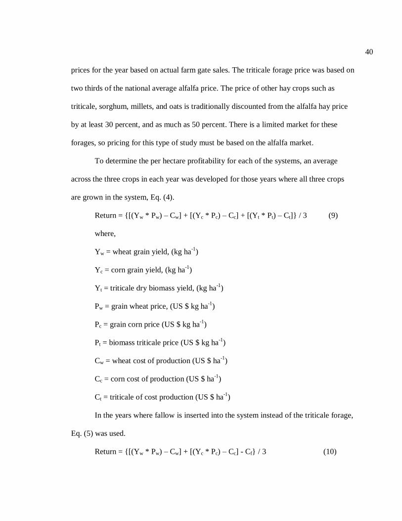
40

prices for the year based on actual farm gate sales. The triticale forage price was based on

two thirds of the national average alfalfa price. The price of other hay crops such as

triticale, sorghum, millets, and oats is traditionally discounted from the alfalfa hay price

by at least 30 percent, and as much as 50 percent. There is a limited market for these

forages, so pricing for this type of study must be based on the alfalfa market.

To determine the per hectare profitability for each of the systems, an average

across the three crops in each year was developed for those years where all three crops

are grown in the system, Eq. (4).

Return = {[(Yw * Pw) – Cw] + [(Yc * Pc) – Cc] + [(Yt * Pt) – Ct]} / 3 (9)

where,

Yw = wheat grain yield, (kg ha-1

)

Yc = corn grain yield, (kg ha-1

)

Yt = triticale dry biomass yield, (kg ha-1

)

Pw = grain wheat price, (US $ kg ha-1

)

Pc = grain corn price (US $ kg ha-1

)

Pt = biomass triticale price (US $ kg ha-1

)

Cw = wheat cost of production (US $ ha-1

)

Cc = corn cost of production (US $ ha-1

)

Ct = triticale of cost production (US $ ha-1

)

In the years where fallow is inserted into the system instead of the triticale forage,

Eq. (5) was used.

Return = {[(Yw * Pw) – Cw] + [(Yc * Pc) – Cc] - Cf} / 3 (10)

41

where,

Yw = wheat grain yield, (kg ha-1

)

Yc = corn grain yield, (kg ha-1

)

Pw = grain wheat price, (US $ kg ha-1

)

Pc = grain corn price (US $ kg ha-1

)

Cw = wheat cost of production (US $ ha-1

)

Cc = corn cost of production (US $ ha-1

)

Cf = fallow cost (US $ ha-1

)

Medians of winter wheat and corn grain yield and spring triticale biomass

modeled for the three flexible rotations and the two fixed rotations, and medians of the

economic return for each cropping system, were analyzed and compared using PROC

GLIMMIX in SAS (SAS Institute, 1985) in order to identify differences.

42

CHAPTER 3. Results and Discussion

3.1. AquaCrop Calibration and Validation

AquaCrop 3.1+ can be used to simulate growth in winter wheat, corn and triticale

in the Central Great Plains. During the calibration with Akron data, good agreement was

found between the observed and predicted values for all three crops (Table 9 and Figures

1-8). The best simulation was grain yield for corn with a d-statistic value of 0.961. A

larger difference was found between the observed and predicted values for spring triticale

ET and corn biomass (d-statistic values of 0.713 and 0.764, respectively). The poor

prediction of spring triticale ET might be explained by the water contents of the surface

60 cm of soil at planting, which was the lowest of all crops evaluated in this study.

Previous studies reported that AquaCrop was very sensitive to initial soil water content

(Garcia-Villa et al., 2009). The prediction of winter wheat and corn grain yield, and

triticale biomass was acceptable, with d-statistic values of 0.921, 0.961, and 0.861,

respectively.

Winter wheat performance was well predicted by the model, which is important to

note since AquaCrop 3.1+ does not account for winter dormancy, which made the

calibration more challenging. In general, AquaCrop was able to simulate, with acceptable

precision, the observed values for all three crops at Akron.

Validation of AquaCrop using data from Sidney indicated that the model was not

accurate in simulating any of the three crops used (Table 10 and Figures 9-16), with d-

values ranging from 0.242 for corn yield to 0.481 for wheat yield and biomass. It is not

clearly understood why AquaCrop did such a poor job modeling the crops at Sidney. The

43

calibration done at Akron was expected to produce similar simulation results at Sidney

without recalibration since the weather and soil environment at Sidney were not greatly

different from Akron. The lower d-values obtained for Sidney could be attributed to the

sensitivity of the program to soil water content. Even though the crops were poorly

predicted at Sidney, we decided to do the multi-year predictions at both locations using

the calibration parameters determined at Akron since they were developed under a fairly

broad range of environmental conditions. Further analysis will likely need to be

performed to determine if there are errors in the field data collected at Sidney, or if

adjustments to some calibration parameters could be made to make the model more

responsive to Sidney conditions. Such an analysis may be helpful in delineating potential

areas of improvement for AquaCrop.

3.2. Multi-year Simulations

Tables 11 and 12 show the different values for winter wheat and corn grain yield

and triticale forage yield predicted by AquaCrop for Akron and Sidney, respectively. In

Tables 13 and 14 it is possible to see that average winter wheat yields were greatest in

WW-C-F and lowest in WW-C-T. For Akron (Table 13), the average values for winter

wheat yield in WW-C-F and WW-C-T were 2670 and 2240 kg ha-1

, respectively. For

Sidney (Table 14), the values were 2450 kg ha-1

for WW-C-F and 2290 kg ha-1

for WW-

C-T. The higher winter wheat grain yield average obtained in WW-C-F was likely the

result of increased soil water after fallow compared to after triticale, 430 and 394 mm,

respectively. The average winter wheat yield tended to decline as the frequency of

summer fallow declined, which agrees with the main objective of summer fallow, which

44

is to increase the total amount of stored soil water to then be used by the following crop

(Moret et al., 2007). This may also explain the increase in yield variability with the

intensification of the cropping system.

Even though winter wheat yield tended to decline as the frequency of summer

fallow declined, and grain yield statistically significant difference was found between the

400 mm flexible fallow system and WW-C-F at Akron (p-value 0.007, Table 15), no

statistical difference was found between these two cropping systems at Sidney (p-value

0.093, Table 16).

Table 17 shows that at Akron, average corn yields were generally not affected by

cropping system, except between WW-C-T and WW-C-F (p-value of 0.001), where WW-

C-F had a greater average corn grain yield. Other statistically significant differences for

corn grain yield were too small to be of any practical significance. A similar situation at

Sidney was found (Table 18).

Average triticale forage yields were not affected by cropping system at either

location (Tables 19 and 20). This might be explained by the fact that winter wheat and

corn crops planted before triticale, likely eliminated any effect that the previous spring

triticale or fallow treatments might have had on soil water storage prior to triticale

planting.

Tables 21 and 22 show the different economic returns for each system at Akron

and Sidney, respectively. At both locations, average income was improved by replacing

summer fallow with spring triticale, but income variability also increased (Tables 23 and

24). Aakre (1991, unpublished data) cited by Dhuyvetter et al. (1996) reported higher

45

income variability in winter wheat-sunflower than in winter wheat-fallow. The increase

in variability in income was attributed to yield variability of the cropping system.

Flexible fallow did not seem to provide much benefit over fixed rotations, i.e.,

flexible fallow did not result in increased yield with little or no increase in income

variability. The exception was Sidney, where the 400 mm threshold had a slightly greater

average return and slightly reduced income variability compared to WW-C-F (Table 24).

From Tables 23 and 24 we can infer that risk-averse growers are likely to prefer

WW-C-F over WW-C-T, but non-risk-averse growers will likely prefer WW-C-T.

Performance of the flexible fallow system using a 400 mm soil water threshold exhibited

a slightly higher average return and slightly smaller income variability than WW-C-F at

Sidney, which may suggest that some risk-averse farmers may prefer flexible fallow with

a high soil water threshold, e.g. 400 mm, over WW-C-F if the cost of obtaining soil water

content information is not prohibitive. However, in general, the economic benefits of

flexible fallow compared to the two fixed cropping systems were minimal.

Tables 25 and 26 show the statistical analysis of the economic returns for the

different systems at both locations. In Figures 17 and 18, it is possible to see the

distribution of the economic returns for each cropping system at Akron and Sidney,

respectively. We can see that at both locations, the economic returns from WW-C-T were

statistically superior to the returns from WW-C-F (p-value of 0.001) for both locations.

Dhuyvetter et al. (1996) reported that the combination of reduced tillage and no-till with

wheat rotations involving sunflower, corn and sorghum had a higher net return than the

traditional winter wheat-fallow rotation in the Great Plains. Nielsen et al. (2005) reported

46

that the increase in precipitation use efficiency on a mass-produced and economic-return

basis was higher in more intense cropping systems involving annual forages.

Even further, WW-C-F was only economically competitive with the flexible

fallow system using a 400 mm soil water threshold. The use of more intense cropping

system than the traditional winter wheat-fallow can reduce the negative impact that

fallow has on the environment. A more intense cropping system not only provides

marketing advantages, but also improves weed control, increases residue retention, and

minimizes insects and diseases associated with monoculture (Nielsen et al., 2008;

Peterson et al., 1993).

47

CHAPTER 4. Conclusions

AquaCrop can be used to simulate ET, which can be used to estimate soil water

content following winter wheat, corn and triticale in the Central Great Plains. AquaCrop

was also effective at simulating grain yield in corn and winter wheat.

The multi-year simulations of flexible fallow using three different soil water

thresholds and two fixed rotations showed that average winter wheat yields were greatest

in WW-C-F and lowest in WW-C-T. However, average annual income was greater

without summer fallow. This suggests that although summer fallow may reduce income

variability, it also likely reduces income potential. Lyon et al. (2004) found that replacing

summer fallow with oat + pea for forage or proso millet reduced subsequent winter wheat

yield, but economic returns were similar to systems with summer fallow.

Even though flexible fallow did not seem to provide much economic benefit over

the two fixed rotations, the adoption of flexible fallow might help to reduce some of the

negative consequences of summer fallow, e.g., soil erosion or the necessity of herbicide

application for weed control by reducing the frequency of summer fallow. Lyon et al.

(2004) mentioned that the elimination or significant reduction of summer fallow use will

not only protect the soil from degradation, but also bring a higher efficiency in water use

and improve the viability of the dryland cropping system in the long-run.

Risk-averse growers are likely to prefer WW-C-F over WW-C-T because of the

reduction in year-to year income variability that summer fallow provides. However, non-

risk-averse growers will likely prefer WW-C-T because of the increase in the average and

total income. For farmers that have animal production incorporated into their farm

48

operations, a cropping system that includes a spring-planted annual forage such as spring

triticale may have greater value than indicated here, where we have included cutting,

baling, and transportation costs for spring triticale in the economic analysis. Grazing

forages can reduce these costs (Clampham et al., 2008) by allowing animals to do some

of the work related to harvesting the forages (Munson et al., 1990).

Our simulations using AquaCrop and 23 yr of historical weather data from Akron,

CO and Sidney, NE suggest that a flexible fallow system, (i.e., a system that uses soil

water in the spring to determine whether to summer fallow prior to planting winter wheat

or plant an annual forage such as triticale as suggested by Felter et al. (2006), provides

little benefit compared to fixed cropping systems with or without summer fallow. Seldom

in this study did flexible fallow provide increased income with little or no increase in

income variability compared to WW-C-F, which is the goal of the flexible fallow system.

This suggests that knowing soil water content in the spring does not insulate growers

sufficiently from the vagaries of seasonal precipitation to significantly reduce crop

production risk in the Central Great Plains. This suggests that growers need to decide if

they are willing to accept greater income variability for the potential of greater income. If

they are, then annual forages can substitute for summer fallow. If not, summer fallow will

lower annual income variability but it will also lower overall income.

The major influence that climate variability has on agriculture is increased

economic risk (Jones et al., 2000). We hypothesized that flexible fallow systems based on

the quantity of soil water in the spring could reduce the production and economic risk

associated with climate variability. However, our crop simulation results provide little

49

support for this hypothesis. Short-term (3 to 4 months) climate forecast combined with

information on stored soil water at planting have been used to help make crop

management decisions in northeast Australia (Stone et al., 1992), which is strongly

influenced by the El Nino southern oscillation. With accurate data input (soil physical

properties, genetic material and weather conditions) modeling can be used as a cropping

system tool (Staggenborg et al., 2005). Perhaps flexible fallow systems will need to

await better climate forecasting skill than is currently available for the Central Great

Plains. Until that time, growers need to make their decisions on the use of summer fallow

based on their level of aversion to risk, i.e. variability, or their level of concern about the

negative soil and environmental consequences of summer fallow.

50

Tables

Table 1. Planting and harvesting dates at Akron, CO for corn, winter wheat and triticale.

Year of

harvest Maize Spring triticale Winter wheat

Planting date Harvest date Planting date Harvest date Planting date Harvest date

2009 12-May-09 6-Oct-09 (dryland) 3-Apr-09 7-May-09 20-Sep-08 20-Jul-09

26-Oct-10 (irrigated)

2010 10-May-10 6-Oct-10 (dryland) 20-Apr-10 * 28-Sep-09 14-Jul-10


2011

17-May-11

13-Oct-11 (dryland)


1-Apr-11

22-Jun-11

22-Sep-10

18-Jul-11

*Not harvested because winter triticale was seeded in error and it failed to vernalize and produce spikes.

51

Table 2. Planting and harvesting dates at Sidney, NE for corn, winter wheat and triticale.

Year of

harvest Maize Spring triticale Winter wheat

Planting date Harvest date Planting date Harvest date Planting date Harvest date

2009 13-May-09 7-Oct-09 13-Apr-09 30-Jun-09 10-Sep-08 15-Jul-09

2010 10-May-10 7-Oct-10 30-Mar-10 22-Jun-10 10-Sep-09 13-Jul-10

2011 * * 1-Apr-11 22-Jun-11 9-Sep-10 19-Jul-11

*No corn was planted at Sidney in 2011.

52

Table 3. Phenological stages at which various soil and crop measurements were taken for each crop.

Spring Triticale

Wheat

Corn

Soil water *LAI Biomass Soil water LAI Biomass Soil water LAI Biomass

Planting Jointing Jointing Emergence Jointing Jointing Planting V8 V8

Emergence Heading Harvest

Mid

November

Mid way to

flowering Flowering V8 Flowering Flowering

Jointing

Mid March Flowering Harvest Flowering Late milk Late milk

Harvest Jointing Dough

Late milk

Flowering

Maturity

Maturity

*LAI= leaf area index .

53

Table 4. Crop parameters used in AquaCrop to simulate winter

wheat.

Parameter Value Units

Initial canopy cover 3.75 %

Canopy growth coefficient (CGC) 2.4 %/day

Maximum canopy cover (CCx) 90 %

Canopy decline coefficient (CDC) 3.1 %/day

Senescence 253 Calendar days

Maturity 296 Calendar days

Duration of flowering 14 Calendar days

From day 1 after sowing to flowering 246 Calendar days

Maximum effective rooting depth 1.8 Meter

Minimum effective rooting depth 0.3 Meter

Soil evaporation coefficient (Ke) 50 %

Crop transpiration coefficient (Kcb) 0.6

Crop water productivity (WP*) 21 g/m2

Reference harvest index (HIo) 27 %

Canopy expansion p-upper 0.3

Canopy expansion p-lower 0.65

Canopy expansion shape factor 3.5

Stomatal closure p-upper 0.45

Stomatal closure shape factor 3.5

Early canopy senescence p-upper 0.75

Early canopy senescence shape factor 3.5

Aeration stress None

Fertility stress None

54

Table 5. Crop parameters used in AquaCrop to simulate

triticale.

Parameter Value Units













Crop water productivity (WP*) 23 g/m2






Stomatal closure shape factor 3.5





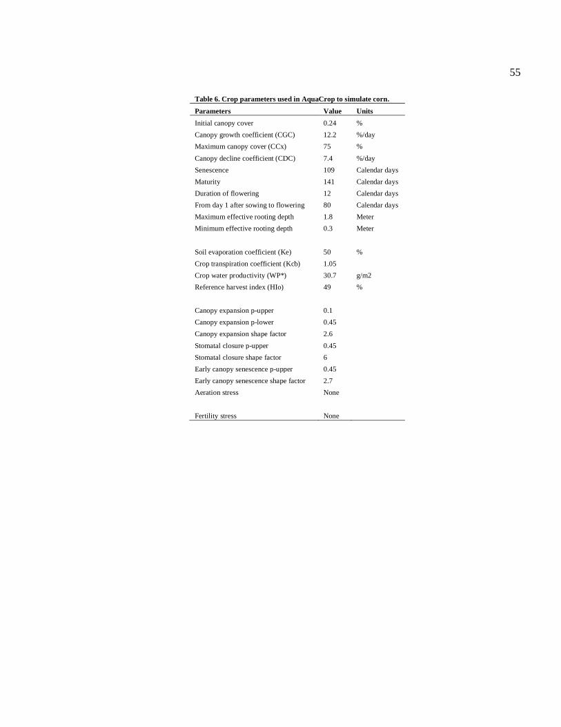
55

Table 6. Crop parameters used in AquaCrop to simulate corn.

Parameters Value Units













Crop water productivity (WP*) 30.7 g/m2






Stomatal closure shape factor 6





56

Table 7. Historical prices for winter wheat, corn, and

spring triticale.

Winter wheat Corn Spring triticale

Year --------------------------US $ kg-1

--------------------------

1988 0.138 0.100 0.079

1989 0.136 0.093 0.077

1990 0.093 0.090 0.071

1991 0.120 0.093 0.061

1992 0.119 0.081 0.064

1993 0.115 0.098 0.073

1994 0.128 0.089 0.075

1995 0.176 0.128 0.071

1996 0.157 0.107 0.083

1997 0.118 0.096 0.087

1998 0.095 0.076 0.072

1999 0.095 0.074 0.065

2000 0.100 0.074 0.073

2001 0.100 0.078 0.085

2002 0.135 0.091 0.082

2003 0.119 0.095 0.074

2004 0.121 0.081 0.080

2005 0.124 0.079 0.085

2006 0.166 0.120 0.092

2007 0.226 0.165 0.112

2008 0.253 0.160 0.135

2009 0.178 0.140 0.092

2010 0.238 0.204 0.100

57

Table 8. Production cost for winter wheat, corn, spring triticale and fallow.

Price index Winter wheat Corn Spring triticale Fallow

Year ------------------------------------------US $ ha-1

-----------------------------------------

1988 92 166 200 170 26

1989 97 175 211 179 27

1990 99 179 216 183 28

1991 100 180 218 185 28

1992 101 182 220 186 29

1993 103 186 224 190 29

1994 106 191 231 196 30

1995 108 195 235 199 31

1996 115 207 250 212 33

1997 118 213 257 218 33

1998 114 206 248 210 32

1999 113 204 246 209 32

2000 115 207 250 212 33

2001 120 217 261 221 34

2002 119 215 259 220 34

2003 124 224 270 229 35

2004 132 238 287 244 37

2005 140 253 305 258 40

2006 150 271 327 277 42

2007 162 292 353 299 46

2008 188 339 409 347 53

2009 183 330 398 338 52

2010 186 336 405 343 53

58

Table 9. Statistics for the comparison between observed and simulated values for seed

yield, final biomass, and crop evapotranspiration (ET) for winter wheat and corn, and

final biomass and crop ET for triticale, for the calibration of AquaCrop for Akron, CO.

Mean

Variable name n Observed Simulated MRE RMSE d statistic

Winter wheat

Yield (kg ha -1

) 20 2180 2010 13 399 0.921

Biomass (kg ha -1

) 20 7340 7820 12 1050 0.938

ET (mm) 20 380 395 9 35.1 0.890

Spring triticale

Biomass (kg ha -1

) 8 4370 4490 28 1140 0.861

ET (mm) 8 160 186 20 36.6 0.713

Corn

Yield (kg ha -1

) 12 3970 4010 20 754 0.961

Biomass (kg ha -1

) 8 11000 12500 24 2460 0.764

ET (mm) 12 430 435 9 41.9 0.886

59

Table 10. Statistics for the comparison between observed and simulated values for seed

yield, final biomass, and crop evapotranspiration (ET) for winter wheat and corn, and

final biomass and crop ET for triticale, for the validation of AquaCrop for Sidney, NE.

Mean

Variable name n Observed Simulated MRE RMSE d statistic

Winter wheat

Yield (kg ha -1

) 12 3390 2530 24 1330 0.481

Biomass (kg ha -1

) 12 11400 9490 17 2880 0.481

ET (mm) 12 534 410 23 135 0.389

Spring triticale

Biomass (kg ha -1

) 6 4480 5500 39 1620 0.420

ET (mm) 6 186 318 38 153 0.461

Corn

Yield (kg ha -1

) 8 6990 7370 4 500 0.242

Biomass (kg ha -1

) 8 16800 15800 13 2910 0.457

ET (mm) 8 472 499 4 30.2 0.398

60

Table 11. Simulated grain yields for winter wheat and corn, and forage yields for triticale, in two fixed rotations [winter wheat-corn-triticale (WW-C-T) and winter wheat-corn-fallow

(WW-C-F) ] and flexible fallow using three different soil water thresholds at planting (350, 375, and 400 mm) to determine when to plant triticale or use fallow at Akron, CO. using

historical weather data from 1988 through 2010. Winter wheat yields are reported at 12.5% moistures; corn yields are reported at 12.5% moisture; triticale yields are reported at 0%

moisture.

WW-C-T

350 mm

375 mm

400 mm

WW-C-F

Year

WW C T

WW C T

WW C T

WW C T

WW C

-------------------------------------------------------------------------------------------------------------kg ha-1

----------------------------------------------------------------------------------------------

1988 2140 3840 4800 2140 3840 4800 2140 3840 4800 2140 3840 4800 2700 3840

1989 1720 3270 4510 1720 3270 **** 1720 3270 **** 1720 3270 **** 2230 4310

1990 1990 7010 4800 2660 7010 4210 2660 7010 **** 2660 7010 **** 2920 7100

1991 2320 4550 4960 2320 4760 4960 2920 4760 **** 2920 4760 **** 2920 4550

1992 2880 6720 4740 2880 6720 4770 3000 7000 **** 3000 7000 **** 3060 6990

1993 2080 6390 4770 2100 6390 4770 2450 6460 **** 2450 6460 **** 2450 6470

1994 1830 4400 4620 1830 4600 4620 2450 4400 4640 2450 4400 **** 2450 4400

1995 3000 2960 4370 3000 2960 4370 3000 2960 **** 3020 2960 **** 3020 2960

1996 3040 7240 4770 3060 7240 **** 2860 7310 **** 2860 7310 **** 2870 7310

1997 2140 6260 4990 2390 6360 4990 2390 6260 5000 2390 6260 **** 2390 6260

1998 1970 5800 4550 1970 6220 4570 2030 6220 4550 2450 6220 **** 2450 6220

1999 1760 7250 4990 1810 7250 **** 1760 7270 **** 2570 7580 **** 2570 7580

2000 2110 4130 4600 2530 4200 4600 2530 4130 4610 2530 4150 4710 2530 4150

2001 2440 6360 5040 2440 6540 5040 2450 6540 4950 2580 6540 **** 2930 6540

2002 1540 70 3760 1580 70 **** 1010 71 **** 1760 75 **** 1750 590

2003 2590 2900 5080 3350 2900 5080 3350 2900 5080 3350 2900 5080 3350 2900

2004 2980 5820 4590 2980 6500 **** 3030 6490 **** 3030 6490 **** 3030 6490

2005 2000 5840 4950 2730 5840 **** 2730 5850 **** 2730 5850 **** 2730 5850

2006 1780 4870 4580 2170 4870 4580 2170 4870 **** 2170 4870 **** 2770 4870

2007 1940 2140 4970 1940 3040 5270 2940 3040 5270 2940 3040 **** 2940 3040

2008 1770 5060 5060 2420 5060 5060 2420 5300 **** 2600 5300 **** 2650 5300

2009 2650 6900 5180 2570 6900 5180 3290 6900 5180 3290 6900 5180 3290 6900

2010 2860 3570 5020 2860 3570 5020 2860 3570 5020 2860 3570 **** 1350 3570

**** Years where fallow was implemented since the water threshold to grow spring triticale was not reached.

60

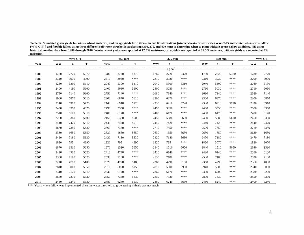
61

Table 12. Simulated grain yields for winter wheat and corn, and forage yields for triticale, in two fixed rotations [winter wheat-corn-triticale (WW-C-T) and winter wheat-corn-fallow

(WW-C-F) ] and flexible fallow using three different soil water thresholds at planting (350, 375, and 400 mm) to determine when to plant triticale or use fallow at Sidney, NE using

historical weather data from 1988 through 2010. Winter wheat yields are reported at 12.5% moistures; corn yields are reported at 12.5% moisture; triticale yields are reported at 0%

moisture.

WW-C-T

350 mm

375 mm

400 mm

WW-C-F

Year

WW C T

WW C T

WW C T

WW C T

WW C

-------------------------------------------------------------------------------------------------------------kg ha-1

----------------------------------------------------------------------------------------------

1988 1780 2720 5370 1780 2720 5370 1780 2720 5370 1780 2720 5370 1780 2720

1989 2310 3930 4990 2310 3930 **** 2310 3930 **** 2310 3930 **** 2200 3930

1990 1280 5300 5310 2040 5300 5310 2040 5300 5310 2040 5300 **** 2040 5130

1991 2400 4190 5600 2400 5030 5600 2400 5030 **** 2710 5030 **** 2710 5030

1992 2750 7140 5300 2750 7140 **** 2680 7140 **** 2680 7140 **** 2680 7140

1993 1960 6870 5610 2300 6870 5610 2300 6870 **** 2300 6870 **** 2300 6870

1994 2140 6910 5720 2140 6910 5720 2330 6910 5720 2330 6910 5720 2330 6910

1995 2490 3350 4975 2490 3350 **** 2490 3350 **** 2490 3350 **** 2500 3350

1996 2510 6170 5310 2400 6170 **** 2400 6170 **** 2400 6170 **** 2400 6170

1997 2250 5380 5600 2450 5380 5600 2450 5380 5600 2450 5380 5600 2450 5380

1998 2440 7420 5510 2440 7420 5510 2440 7420 **** 2440 7420 **** 2440 7420

1999 2660 7350 5620 2660 7350 **** 2710 7350 **** 2500 7350 **** 2710 7350

2000 2330 1650 5650 2630 1650 5650 2630 1650 5650 2630 1650 **** 2630 1650

2001 2420 7180 5630 2420 7180 5630 2420 7180 5630 2470 7180 **** 2470 7180

2002 1820 795 4690 1820 795 4690 1820 795 **** 1820 3070 **** 1820 3070

2003 1870 1510 5650 1870 1510 5650 2840 1510 5650 2840 1510 5650 2840 1510

2004 2410 4910 5520 2410 4740 **** 2410 6140 **** 2420 6140 **** 2550 6130

2005 2380 7180 5520 2530 7180 **** 2530 7180 **** 2530 7180 **** 2530 7180

2006 2210 4790 5180 2320 4790 5180 2360 4790 5180 2360 4790 **** 2360 4800

2007 2810 5000 5950 2810 5000 5950 2810 5000 5950 2940 5000 **** 2940 5000

2008 2340 6170 5610 2340 6170 **** 2340 6170 **** 2380 6200 **** 2380 6200

2009 2680 7330 5830 2850 7330 5830 2850 7330 **** 2850 7330 **** 2850 7330

2010 2480 6240 5630 2480 6240 5630 2480 6240 5630 2480 6240 **** 2400 6240

**** Years where fallow was implemented since the water threshold to grow spring triticale was not reach.

61

62

Table 13. Summary of simulated grain yield for winter wheat and corn and forage yield for triticale for Akron, CO. Winter wheat yields are reported at 12.5% moistures; corn

yields are reported at 12.5% moisture; triticale yields are reported at 0% moisture.

WW-C-T 350mm 375 mm 400mm WW-C-F

WW C T WW C T WW C T WW C T WW C T

--------------------------------------------------------------------------------------------------kg ha-1

---------------------------------------------------------------------------------------------

Average 2240 4930 4770 2410 5050 4820 2530 5060 4910 2630 5080 4940 2670 5140 --

Total 51500 113000 111000 55500 116000 81900 58200 116000 49100 60500 117000 19800 61400 118000 --

SD 469 1870 310 482 1850 294 551 1870 249 422 1890 221 458 1800 --

Minimum 1543 1543 1543 1543 1543 1543 1543 1543 1543 1543 1543 1543 1543 1543 --

Maximum 3042 3042 3042 3042 3042 3042 3042 3042 3042 3042 3042 3042 3042 3042 --

Range 1500 1500 1500 1500 1500 1500 1500 1500 1500 1500 1500 1500 1500 1500 --

62

63

Table 14. Summary of simulated grain yield for winter wheat and corn and forage yield for triticale for Sidney, NE. Winter wheat yields are reported at 12.5% moistures; corn yields

are reported at 12.5% moisture; triticale yields are reported at 0% moisture.


WW C T WW C T WW C T WW C T WW C T

-------------------------------------------------------------------------------------------------------kg ha-1

-----------------------------------------------------------------------------------------------

Average 2290 5200 5470 2370 5220 5530 2430 5290 5570 2240 5390 5580 2450 5380 --

Total 52700 119000 126000 54600 120000 82900 55800 122000 55700 56100 124000 22300 56300 124000 --

SD 356 2050 293 291 2040 301 278 2050 224 286 1870 1870 296 1870 --

Minimum 1283 1283 1283 1283 1283 1283 1283 1283 1283 1283 1283 1283 1283 1283 --

Maximum 2813 2813 2813 2813 2813 2813 2813 2813 2813 2813 2813 2813 2813 2813 --

Range 1530 1530 1530 1530 1530 1530 1530 1530 1530 1530 1530 1530 1530 1530 --

63

64

Table 15. Statistical comparison of average winter wheat grain yield predicted for each cropping

system at Akron, CO.

Water threshold Estimate Std. error DF t-value Pf > |t|

WW-C-T vs. 350 mm -80 62.3 52 -1.24 0.222

WW-C-T vs. 375 mm -150 68.6 52 -2.19 0.033

WW-C-T vs. 400 mm -313 70.4 52 -4.44 <.0001

WW-C-T vs. WW-C-F -545 74.9 52 -7.27 <.0001

350 mm vs. 375 mm -73 70.8 52 -1.03 0.307

350 mm vs. 400 mm -236 73.5 52 -3.21 0.002

350 mm vs. WW-C-F -468 79.3 52 -5.90 <.0001

375 mm vs. 400 mm -163 75.3 52 -2.16 0.035

375 mm vs. WW-C-F -395 83.1 52 -4.75 <.0001

400 mm vs. WW-C-F -232 82.9 52 -2.79 0.007

65

Table 16. Statistical comparison of average winter wheat grain yield predicted for each

cropping system at Sidney, NE.

Water threshold Estimate Std Error DF t-value Pf > |t|

WW-C-T vs. 350 mm -37 40 52 -0.94 0.353

WW-C-T vs. 375 mm -75 41 52 -1.83 0.073

WW-C-T vs. 400 mm -150 44 52 2.42 0.019

WW-C-T vs. W-C-F -197 46 52 -4.25 <.0001

350 mm vs. 375 mm -39 43 52 -0.89 0.337

350 mm vs. 400 mm -68 46 52 -1.50 0.14

350 mm vs. W-C-F -160 50 52 -3.23 0.002

375 mm vs. 400 mm -30 45 52 -0.66 0.514

375 mm vs. W-C-F -121 51 52 -2.37 0.021

400 mm vs. W-C-F -92 54 52 -1.71 0.093

66

Table 17. Statistical comparison of average corn grain yield predicted for each cropping



WW-C-T vs. 350 mm -121.0 58.9 52 -2.05 0.045

WW-C-T vs. 375 mm -129.4 64.9 52 -1.99 0.051

WW-C-T vs. 400 mm -149.6 66.7 52 -2.24 0.029

WW-C-T vs. WW-C-F -243.2 71.0 52 -3.43 0.001

350 mm vs. 375 mm -8.5 66.9 52 -0.13 0.900

350 mm vs. 400 mm -28.6 69.5 52 -0.41 0.682

350 mm vs. WW-C-F -122.3 75.1 52 -1.63 0.110

375 mm vs. 400 mm -20.2 71.0 52 -0.28 0.778

375 mm vs. WW-C-F -113.8 78.7 52 -1.45 0.154

400 mm vs. WW-C-F -93.6 78.4 52 -1.19 0.238

67

Table 18. Statistical comparison of average corn grain yield predicted for each cropping

system at Sidney, NE. Water threshold Estimate Std Error DF t-value Pf > |t|

WW-C-T vs. 350 mm -14.5 160.9 52 -0.14 0.893

WW-C-T vs. 375 mm -118.2 112.5 52 -1.05 0.298

WW-C-T vs. 400 mm -304.1 118.6 52 -2.57 0.013

WW-C-T vs. W-C-F -94.9 126.1 52 -0.75 0.455

350 mm vs. 375 mm -103.7 118.0 52 -0.88 0.383

350 mm vs. 400 mm -289.7 124.0 52 -2.34 0.023

350 mm vs. W-C-F -80.4 134.7 52 -0.6 0.553

375 mm vs. 400 mm -185.9 122.9 52 -1.51 0.136

375 mm vs. W-C-F 23.3 139.1 52 0.17 0.867

400 mm vs. W-C-F 209.3 145.8 52 1.43 0.157

68

Table 19. Statistical comparison of average triticale biomass yield predicted for each cropping



WW-C-T vs. 350 mm 8.6 32.3 26 0.27 0.792

WW-C-T vs. 375 mm -9.0 39.9 26 -0.23 0.823

WW-C-T vs. 400 mm -31.4 58.1 26 -0.54 0.593

350 mm vs. 375 mm -17.6 40.0 26 -0.44 0.664

350 mm vs. 400 mm -40.0 58.2 26 -0.69 0.497

375 mm vs. 400 mm -22.4 59.8 26 -0.38 0.710

69

Table 20. Statistical comparison of average spring triticale biomass yield predicted for each

cropping system at Sidney, NE.


WW-C-T vs. 350 mm -2E-05 0.042 26 0 1

WW-C-T vs. 375 mm -3E-05 0.049 26 0 1

WW-C-T vs. 400 mm -3E-05 0.071 26 0 1

350 mm vs. 375 mm -7E-06 0.049 26 0 1

350 mm vs. 400 mm -8E-06 0.071 26 0 1

375 mm vs. 400 mm -2E-06 0.072 26 0 1

70

Table 21. Economic returns for simulated grain yields for winter wheat and corn, and forage yields for triticale, in two fixed rotations [winter wheat-corn-triticale

(WW-C-T) and winter wheat-corn-fallow (WW-C-F)] and flexible fallow using three different soil water thresholds at planting (350, 375, 400 mm) to determine when to

plant triticale or use fallow at Akron, CO. using historical weather data from 1988 through 2010.

375 mm 400 mm WW-C-F

Year WW C T System WW C T System WW C T System WW C T System WW C T System

-----------------------------------------------------------------------------------------------US $ ha-1

------------------------------------------------------------------------------------------------

1988 129 184 209 174 129 184 209 174 129 184 209 174 129 184 209 174 206 184 -26 121

1989 58 92 166 106 58 92 -27 41 58 92 -27 41 58 92 -27 41 127 189 -27 96

1990 6 414 157 192 68 414 115 199 68 414 -28 151 68 414 -28 151 92 422 -28 162

1991 97 207 117 140 97 226 117 147 169 226 -28 122 169 226 -28 122 169 207 -28 116

1992 160 328 116 201 160 328 118 202 174 350 -29 165 174 350 -29 165 180 349 -29 167

1993 53 404 158 205 55 404 158 206 96 411 -29 159 96 411 -29 159 96 413 -29 160

1994 43 160 152 118 43 178 152 124 121 160 152 145 121 160 -30 84 122 160 -30 84

1995 334 142 112 196 334 142 112 196 333 142 -31 148 338 142 -31 150 338 142 -31 150

1996 271 522 184 325 273 522 -33 254 243 529 -33 246 243 529 -33 246 243 529 -33 247

1997 39 341 218 200 68 351 218 213 68 341 218 209 68 341 -33 126 68 341 -33 125

1998 -19 195 117 97 -19 227 118 109 -13 227 118 111 26 227 -32 74 26 227 -32 74

1999 -37 293 118 125 -32 293 -32 76 -37 295 -32 75 40 317 -32 108 40 317 -32 108

2000 4 57 122 61 46 62 122 77 46 57 122 75 46 58 122 75 46 58 -33 24

2001 27 232 207 155 27 245 207 160 27 245 207 160 40 245 -34 84 76 245 -34 96

2002 -6 -253 87 -57 -1 -253 -34 -96 -78 -253 -34 -121 23 -252 -34 -88 22 -206 -34 -72

2003 84 6 147 79 174 6 147 109 174 6 147 109 174 6 147 109 174 6 -35 48

2004 122 184 125 144 122 239 -37 108 128 239 -37 110 128 239 -37 110 128 239 -37 110

2005 -5 155 162 104 86 155 -40 67 86 155 -40 67 86 155 -40 67 86 155 -40 67

2006 25 256 146 142 90 256 146 164 90 256 -42 101 90 256 -42 101 190 256 -42 135

2007 147 1 257 135 147 149 290 195 372 149 290 271 372 149 -46 158 372 149 -46 158

2008 109 399 335 281 274 399 334 336 274 438 -53 219 319 438 -53 235 333 438 -53 239

2009 140 566 140 282 127 566 140 278 255 566 140 320 255 566 140 320 255 566 -52 256

2010 346 323 160 277 346 323 160 277 346 323 160 277 346 323 -53 206 -14 323 -53 86

70

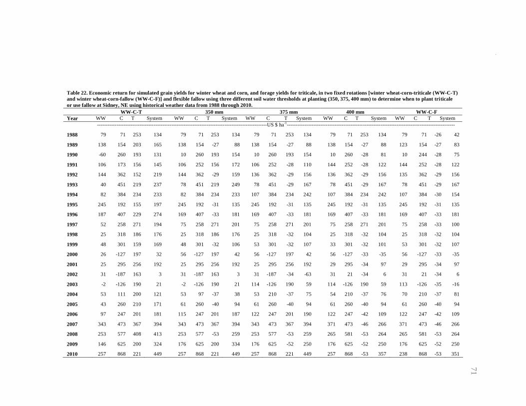
71

Table 22. Economic return for simulated grain yields for winter wheat and corn, and forage yields for triticale, in two fixed rotations [winter wheat-corn-triticale (WW-C-T)

and winter wheat-corn-fallow (WW-C-F)] and flexible fallow using three different soil water thresholds at planting (350, 375, 400 mm) to determine when to plant triticale

or use fallow at Sidney, NE using historical weather data from 1988 through 2010.

WW-C-T 350 mm 375 mm 400 mm WW-C-F

Year WW C T System WW C T System WW C T System WW C T System WW C T System

------------------------------------------------------------------------------------------------US $ ha-1

-----------------------------------------------------------------------------------------------

1988 79 71 253 134 79 71 253 134 79 71 253 134 79 71 253 134 79 71 -26 42

1989 138 154 203 165 138 154 -27 88 138 154 -27 88 138 154 -27 88 123 154 -27 83

1990 -60 260 193 131 10 260 193 154 10 260 193 154 10 260 -28 81 10 244 -28 75

1991 106 173 156 145 106 252 156 172 106 252 -28 110 144 252 -28 122 144 252 -28 122

1992 144 362 152 219 144 362 -29 159 136 362 -29 156 136 362 -29 156 135 362 -29 156

1993 40 451 219 237 78 451 219 249 78 451 -29 167 78 451 -29 167 78 451 -29 167

1994 82 384 234 233 82 384 234 233 107 384 234 242 107 384 234 242 107 384 -30 154

1995 245 192 155 197 245 192 -31 135 245 192 -31 135 245 192 -31 135 245 192 -31 135

1996 187 407 229 274 169 407 -33 181 169 407 -33 181 169 407 -33 181 169 407 -33 181

1997 52 258 271 194 75 258 271 201 75 258 271 201 75 258 271 201 75 258 -33 100

1998 25 318 186 176 25 318 186 176 25 318 -32 104 25 318 -32 104 25 318 -32 104

1999 48 301 159 169 48 301 -32 106 53 301 -32 107 33 301 -32 101 53 301 -32 107

2000 26 -127 197 32 56 -127 197 42 56 -127 197 42 56 -127 -33 -35 56 -127 -33 -35

2001 25 295 256 192 25 295 256 192 25 295 256 192 29 295 -34 97 29 295 -34 97

2002 31 -187 163 3 31 -187 163 3 31 -187 -34 -63 31 21 -34 6 31 21 -34 6

2003 -2 -126 190 21 -2 -126 190 21 114 -126 190 59 114 -126 190 59 113 -126 -35 -16

2004 53 111 200 121 53 97 -37 38 53 210 -37 75 54 210 -37 76 70 210 -37 81

2005 43 260 210 171 61 260 -40 94 61 260 -40 94 61 260 -40 94 61 260 -40 94

2006 97 247 201 181 115 247 201 187 122 247 201 190 122 247 -42 109 122 247 -42 109

2007 343 473 367 394 343 473 367 394 343 473 367 394 371 473 -46 266 371 473 -46 266

2008 253 577 408 413 253 577 -53 259 253 577 -53 259 265 581 -53 264 265 581 -53 264

2009 146 625 200 324 176 625 200 334 176 625 -52 250 176 625 -52 250 176 625 -52 250

2010 257 868 221 449 257 868 221 449 257 868 221 449 257 868 -53 357 238 868 -53 351

71

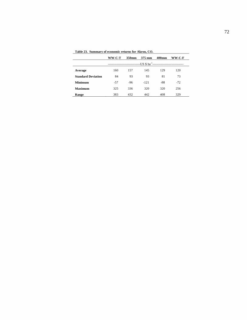
72

Table 23. Summary of economic returns for Akron, CO.


------------------------------US $ ha-1

-----------------------------

Average 160 157 145 129 120

Standard Deviation 84 93 93 81 73

Minimum -57 -96 -121 -88 -72

Maximum 325 336 320 320 256

Range 383 432 442 408 329

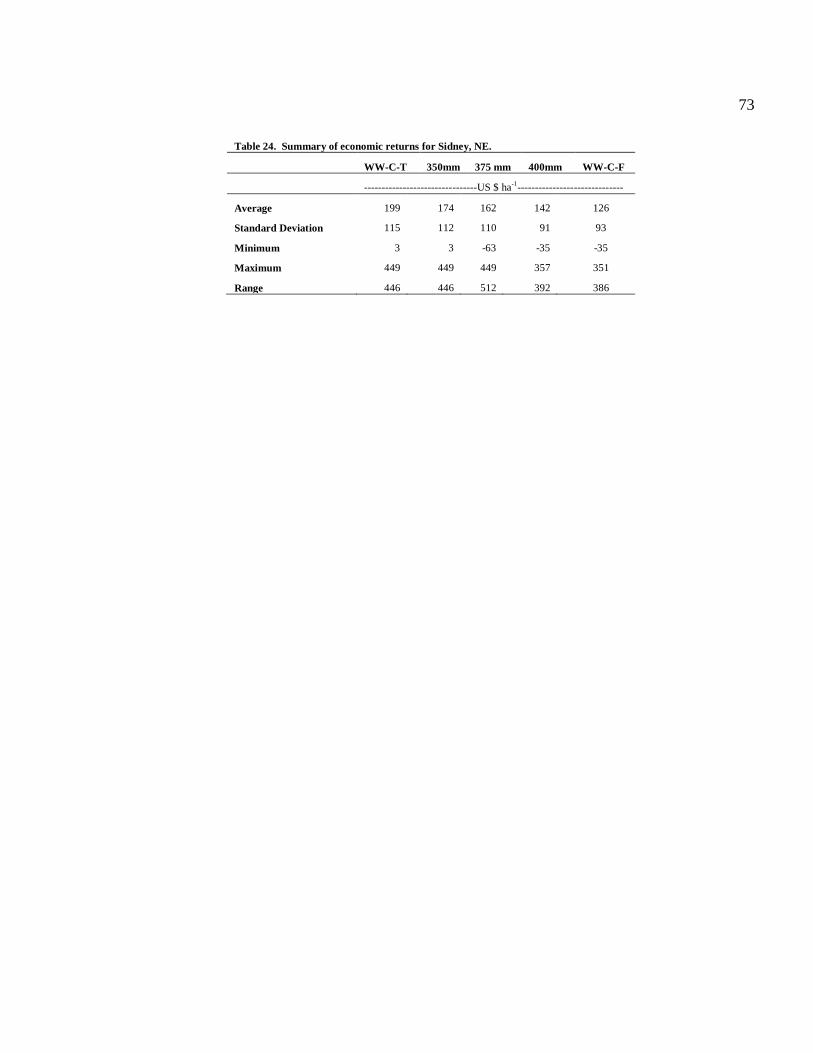
73

Table 24. Summary of economic returns for Sidney, NE.


--------------------------------US $ ha-1

------------------------------

Average 199 174 162 142 126

Standard Deviation 115 112 110 91 93

Minimum 3 3 -63 -35 -35

Maximum 449 449 449 357 351

Range 446 446 512 392 386

74

Table 25. Statistical comparisons of average differences in economic returns between

cropping systems at Akron, CO.

Water threshold US $ ha -1

Std Error DF t-value Pf > |t|

WW-C-T vs. 350 mm 2.9 8.68 88 0.34 0.733

WW-C-T vs. 375 mm 15.1 8.68 88 1.74 0.085

WW-C-T vs. 400 mm 30.6 8.68 88 3.53 <0.001

WW-C-T vs. W-C-F 40.3 8.68 88 4.63 <0.001

350 mm vs. 375 mm 12.1 8.68 88 1.4 0.165

350 mm vs. 400 mm 27.7 8.68 88 3.18 0.002

350 mm vs. W-C-F 37.3 8.68 88 4.29 <0.001

375 mm vs. 400 mm 15.5 8.68 88 1.79 0.008

375 mm vs. W-C-F 25.1 8.68 88 2.89 0.005

400 mm vs. W-C-F 9.6 8.68 88 1.11 0.271

75

Table 26. Statistical comparisons of average differences in economic returns between

cropping systems at Sidney, NE.

Water threshold US $ ha-1

Std Error DF t-value Pf > |t|

WW-C-T vs. 350 mm 25.0 9.24 88 2.71 0.008

WW-C-T vs. 375 mm 37.2 9.24 88 4.03 <0.001

WW-C-T vs. 400 mm 57.5 9.24 88 6.22 <0.001

WW-C-T vs. W-C-F 73.2 9.24 88 7.93 <0.001

350 mm vs. 375 mm 12.2 9.24 88 1.32 0.189

350 mm vs. 400 mm 32.5 9.24 88 3.51 <0.001

350 mm vs. W-C-F 48.2 9.24 88 5.22 <0.001

375 mm vs. 400 mm 20.2 9.24 88 2.19 0.031

375 mm vs. W-C-F 36.0 9.24 88 3.9 <0.001

400 mm vs. W-C-F 15.8 9.24 88 1.71 0.091

76

Figures

Yield Corn at Akron, CO

Observed yield (kg ha-1

)

0 1000 2000 3000 4000 5000 6000 7000 8000

Sim

ula

ted y

ield

(kg h

a-1

)

0

2000

4000

6000

8000

d=0.96

1:1 line

Figure 1. Simulated vs. observed yield values for corn at Akron, CO.

77

Biomass Corn at Akron, CO

Observed biomass (kg ha-1

)

6000 8000 10000 12000 14000 16000 18000

Sim

ula

ted b

iom

ass(k

g h

a-1

)

6000

8000

10000

12000

14000

16000

18000

d=0.76

1:1 line

Figure 2. Simulated vs. observed biomass values for corn at Akron, CO.

78

ET Corn at Akron, CO

Observed ET (mm)

300 350 400 450 500 550

Sim

ula

ted

ET

(m

m)

300

350

400

450

500

550

d=0.89

1:1 line

Figure 3. Simulated vs. observed ET values for corn at Akron, CO.

79

Biomass Triticale at Akron, CO


)

0 2000 4000 6000 8000

Sim

ula

ted b

iom

ass(k

g h

a-1

)

0

1000

2000

3000

4000

5000

6000

7000

8000

d=0.86

1:1 line

Figure 4. Simulated vs. observed biomass values for triticale at Akron, CO.

80

ET Triticale Akron, CO

Observed ET (mm)

100 120 140 160 180 200 220 240

Sim

ula

ted E

T (

mm

)

100

120

140

160

180

200

220

240

d=0.71

1:1 line

Figure 5. Simulated vs. observed ET values for triticale at Akron, CO.

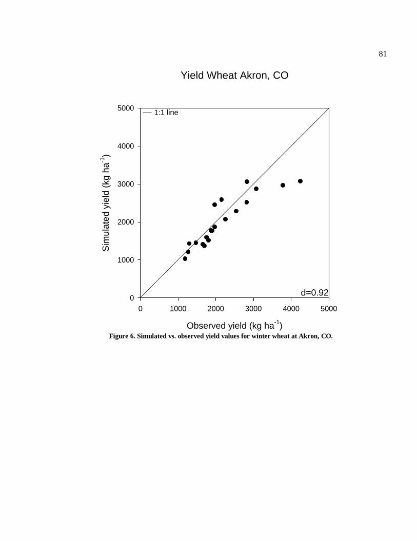
81

Yield Wheat Akron, CO


)

0 1000 2000 3000 4000 5000

Sim

ula

ted

yie

ld (

kg

ha

-1)

0

1000

2000

3000

4000

5000

d=0.92

1:1 line

Figure 6. Simulated vs. observed yield values for winter wheat at Akron, CO.

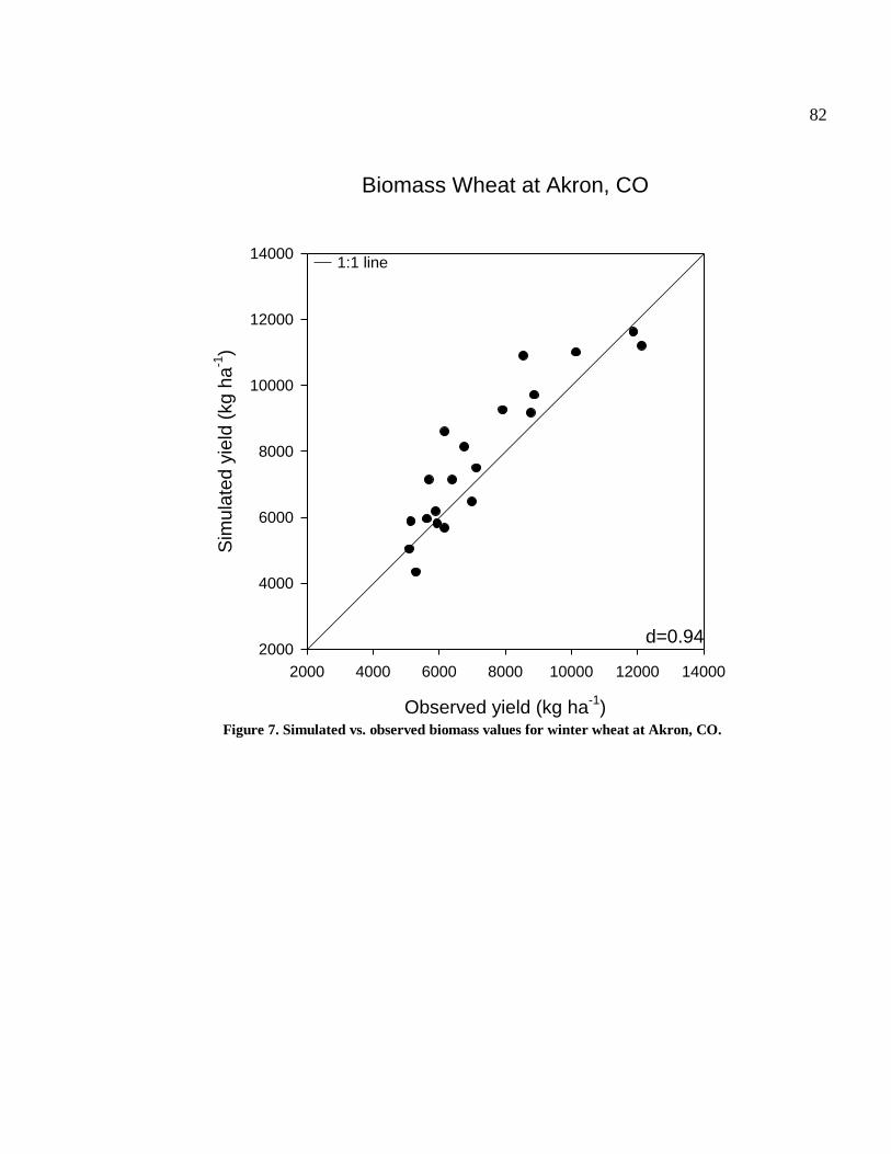
82

Biomass Wheat at Akron, CO


)

2000 4000 6000 8000 10000 12000 14000

Sim

ula

ted y

ield

(kg h

a-1

)

2000

4000

6000

8000

10000

12000

14000

d=0.94

1:1 line

Figure 7. Simulated vs. observed biomass values for winter wheat at Akron, CO.

83

ET Wheat at Akron, CO

Observed ET (mm)

200 300 400 500 600

Sim

ula

ted

ET

(m

m)

200

300

400

500

600

d=0.89

1:1 line

Figure 8. Simulated vs. observed ET values for winter wheat at Akron, CO.

84

Yield Corn at Sidney, NE


)

3000 4000 5000 6000 7000 8000

Sim

ula

ted

yie

ld (

kg

ha

-1)

3000

4000

5000

6000

7000

8000

d=0.24

1:1 line

Figure 9. Simulated vs. observed yield values for corn at Sidney, NE.

85

Biomass Corn at Sidney, NE


)

10000 12000 14000 16000 18000 20000 22000

Sim

ula

ted b

iom

ass(k

g h

a-1

)

10000

12000

14000

16000

18000

20000

22000

d=0.46

1:1 line

Figure 10. Simulated vs. observed biomass values for corn at Sidney, NE.

86

ET Corn at Sidney, NE

Observed ET (mm)

380 400 420 440 460 480 500

Sim

ula

ted

ET

(m

m)

380

400

420

440

460

480

500

d=0.39

1:1 line

Figure 11. Simulated vs. observed ET values for corn at Sidney, NE.

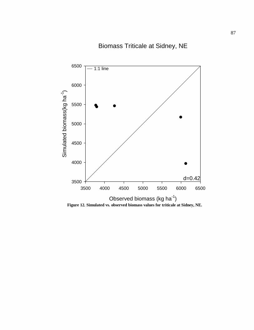
87

Biomass Triticale at Sidney, NE


)

3500 4000 4500 5000 5500 6000 6500

Sim

ula

ted

bio

ma

ss(k

g h

a-1

)

3500

4000

4500

5000

5500

6000

6500

d=0.42

1:1 line

Figure 12. Simulated vs. observed biomass values for triticale at Sidney, NE.

88

ET Triticale at Sidney, NE

Observed ET (mm)

150 200 250 300 350 400 450

Sim

ula

ted

ET

(m

m)

150

200

250

300

350

400

450

d=0.46

1:1 line

Figure 13. Simulated vs. observed ET values for triticale at Sidney, NE.

89

Yield Wheat at Sidney, NE


)

1000 2000 3000 4000 5000 6000

Sim

ula

ted y

ield

(kg h

a-1

)

1000

2000

3000

4000

5000

6000

d=0.48

1:1 line

Figure 14. Simulated vs. observed yield values for winter wheat at Sidney, NE.

90

Biomass Wheat at Sideney, NE


)

8000 8500 9000 9500 10000 10500 11000

Sim

ula

ted

bio

ma

ss(k

g h

a-1

)

8000

8500

9000

9500

10000

10500

11000

d=0.48

1:1 line

Figure 15. Simulated vs. observed biomass values for winter wheat at Sidney, NE.

91

ET Wheat at Sidney, NE

Observed ET (mm)

300 400 500 600 700

Sim

ula

ted

ET

(m

m)

300

400

500

600

700

d=0.39

1:1 line

Figure 16. Simulated vs. observed ET values for winter wheat at Sidney, NE.

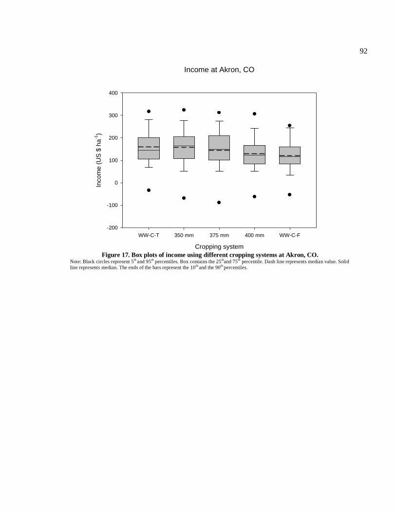
92

Income at Akron, CO

Cropping system


Inco

me

(U

S $

ha

-1)

-200

-100

0

100

200

300

400

Figure 17. Box plots of income using different cropping systems at Akron, CO.

Note: Black circles represent 5th

and 95th percentiles. Box contains the 25

thand 75

th percentile. Dash line represents median value. Solid

line represents median. The ends of the bars represent the 10th

and the 90th

percentiles.

93

Income at Sidney, NE

Cropping system


Yie

ld (

kg

ha

-1)

-100

0

100

200

300

400

500

Figure 18. Box plots of income using different cropping systems at Sidney, NE. Note: Black circles represent 5

th and 95

th percentiles. Box contains the 25

thand 75



and the 90th

percentiles.

94

References

Aase, J.K., and J.L. Pikul Jr. 2000. Water use in a modified summer fallow system on

semiarid northern Great Plains. Agric. Water Manage. 43:45-357.

Angus J.F., and A.F. van Herwaarden. 2001. Increasing water use and water use

efficiency in dryland wheat. Agron. J. 93:290-298.

Araya, A., S. Habtu, K. M. Hadgu, A. Kebede, and T. Dejene. 2010. Test of AquaCrop

model in simulating biomass and yield of water deficient and irrigated barley (Hordeum

vulgare). Agric. Water Manage. 97:1838-1846.

Black, A.L., P.L. Brown, F.H. Siddoway. 1981. Dryland cropping strategies for efficient

water-use to control saline seeps in the northern Great Plains, U.S.A. Agric. Water

Manage. 4: 295-311.

Brown, P.L., A.D. Halvorson, F.H. Siddoway, R.E. Mayland, and M.R. Miller. 1983.

Saline-seep diagnosis, control, and reclamation. USDA Conserv. Res. Rep. 30. US Gov.

Print. Office, Washington, DC.

Burt, O.R., and M.S. Stauber. 1989. Dryland cropping decision theory with application to

saline seep control. J. Prod. Agric. 2:47-57.

Daugovish, O., D.J. Lyon, and D.D. Baltensperger. 1999. Cropping systems to control

winter annual grasses in winter wheat (Triticum aestivium). Weed Technol. 13:120-126.

Dhuyvetter, K.C., C.R. Thompson, C.A. Norwood, and A.D. Halvorson. 1996.

Economics of dryland cropping systems in the Great Plains: A review. J. Prod. Agric.

9:216–222.

FAO-Natural Resources and Environmental Department. 2011. Software AquaCrop.

Available at http://www.fao.org/nr/water/infores_databases_aquacrop.html (verified

2011). FAO Rome, Italy.

Farahani, H.J., G. Izzi, T. Y. Oweis. 2009. Parameterization and evaluation of AquaCrop

model for full and deficit irrigated cotton. Agron. J. 101:468-476.

Farahani, H.J., G.A. Peterson, and D.G. Westfall. 1998. Dryland cropping intensification:

A fundamental solution to efficient use of precipitation. Adv. Agron. 64:197-223.

Felter, D.G., D.J. Lyon, and D.C. Nielsen. 2006. Evaluating crops for flexible summer

fallow cropping system. Agron. J. 98:1510-1517.

Garcia-Vila, M., E. Fereres, L. Mateos, F. Orgaz, and P. Steduto. 2009. Deficit irrigation

optimization of cotton with AquaCrop. Agron. J. 101:477-487.

http://www.fao.org/nr/water/infores_databases_aquacrop.html

95

Geerts, S., D. Raes, and M. Garcia. 2010. Using AquaCrop to derive deficit irrigation

schedules. Agric. Water Manag. 98:213-216.

Hanson, J.D., M. A. Liebig, S. D. Merrill, D. L. Tanaka, J. M. Krupinsky, and D. E.

Scott. 2007. Dynamic cropping systems: Increasing adaptability amid an uncertain future.

Agron. J. 99:939-943.

Heng, L. K., T. Hsiao, S. Evett, T. Howell, and P. Steduto. 2009. Validating the FAO

AquaCrop model for irrigated and water deficient field corn. Agron. J. 101:488-498.

Hsiao, T. C., L. Heng, P. Steduto, B. Rojas-Lara, D. Raes, and E. Fereres. 2009.

AquaCrop The FAO crop model to simulate yield response to water: III. Parameterization

and testing for corn. Agron. J. 101:448-459.

ICASA- DSSAT Version 4. Introduction. Available at

http://www.icasa.net/dssat/index.html. (verified 26 Oct. 2011). ICASA, Honolulu, HI.

Johnson, R.G., and M.B. Ali. 1982. Economics of wheat-fallow cropping systems in

western North Dakota. Western J. of Agric. Econ. 7:67-77

Jones, J. W., J.W. Hansen, F.S. Royce, and C. D. Messina. 2000. Potential benefits of

climate forecasting to agriculture. Agric. Ecosys. Environ. 82:169-184

Lyon, D. J., and R. L. Anderson. 1993. Crop response to fallow applications of atrazine

and clomazone. Weed Technol. 7:949-953.

Lyon, D.J., D.D. Baltensperger, J.M. Blumenthal, P.A. Burgener, and R.M. Harveson.

2004. Eliminating summer fallow reduces winter wheat yields, but not necessarily system

profitability. Crop Sci. 44:855–86.

Lyon, D.J., D.C. Nielsen, D.G. Felter, and P. Burgener. 2007. Choice of summer fallow

replacement crops impacts subsequent winter wheat. Agron. J. 99:578–584.

Lyon, D.J., F.Boa, and T.J. Arkebauer. 1995. Water-yield relations of several spring

planted dryland crops following winter wheat. J. Prod. Agric. 8:281-286.

Lyon, D.J., G. L. Hammer, G. B. McLean, and J.M. Blumenthal. 2003. Simulation

supplements field studies to determine no-till dryland corn population recommendations

for semiarid western Nebraska. Agron. J. 95:884-891.

Mupangwa, W., J. Dimes, S. Walker, and S. Twomlow. 2011. Measuring and simulating

corn (Zea mays L.) yield responses to reduced tillage and mulching under semi-arid

conditions. Agric. Sci. 2:167-174.

http://www.icasa.net/dssat/index.html

96

McGee, E.A., G. A. Peterson, and D.G. Westfall. 1997. Water storage efficiency in no-till

cropping systems. J. Soil Water Conserv. 52:131-136.

Moret, D., I. Braud, and J.L. Arrue. 2006. Water balance simulation of a dryland soil

during fallow under conventional and conservation tillage in semiarid Argon, Northeast

Spain. Soil Till. Res. 92:251-263.

Moeller, C., M. Pala, A. M. Manschadi, H. Meinke, and J. Sauerborn. 2007. Australian J.

of Agric. Res. 58:75-86.

Munson, C. L., J. C. Whittier, D. N. Schutz, and R. L. Anderson. 1990. Reducing annual

cow cost by grazing windrowed millet. The Prof. Animal Scientist 15:40-45.

Nielsen, D. C., P. W. Unger, and P. R. Miller. 2005. Efficient water use in dryland

cropping systems in the Great Plains. Agron. J. 97:364-372.

Nielsen, D. C., and M. F. Vigil. 2010. Precipitation storage efficiency during fallow in

wheat-fallow systems. Agron. J. 102:537-543.

Nielsen, D.C., M.F. Vigil, and J.G. Benjamin. 2009. The variable response of dryland

corn yield to soil water content at planting. Agric. Water Manage. 96:330-336.

Nielsen, D.C., R.L. Anderson, R.A. Bowman, R.M. Aiken, M.F. Vigil, and J.G.

Benjamin. 1999. Winter wheat and proso millet yield reduction due to sunflower in

rotation. J. Prod. Agric. 12:193-197.

Nielsen, D.C., M.F. Vigil, R.L. Anderson, R.A. Bowman, J.G. Benjamin, and A.D.

Halvorson. 2002. Cropping system influence on planting water content and yield of

winter wheat. Agron. J. 94:962-967.

Nielsen, D.C., and F. J. Calderon. 2011. Fallow effects on soil. p. 287-300 In J.L.

Hatfield and T.J. Sauer (ed.) Soil management: building a stable base for agriculture.

ASA and SSSA, Madison, WI.

Peterson, G.A., A.D. Halvorson, J.L. Havlin, O.R. Jones, D.J. Lyon, and D.L. Tanaka.

1998. Reduced tillage and increasing cropping intensity in the Great Plains conserves soil

C. Soil Till. Res. 47:207–218.

Peterson, G.A., D.G. Westfall, and C.V. Cole. 1993. Agroecosystem approach to soil and

crop management research. Soil Sci. Soc. Am. J. 57:1354-1360.

Peterson, G.A., A.J. Schlegel, D.L. Tanaka and O. R. Jones. 1996. Precipitation use

efficiency as affected by cropping and tillage system. J. Prod. Agric. 9:180-186.

97

Peterson, G.A., D.G. Westfall, N.E. Toman, and R.L. Anderson. 1993. Sustainable

dryland cropping system: Economic analysis. USDA-ARS Tech. Bull. TB93-3.

Raes, D., P. Steduto, T. C. Hsiao, and E. Fereres. 2009. AquaCrop The FAO crop model

to simulate yield response to water: II. Main algorithms and software description. Agron.

J. 101:438-447.

Raes, D., P. Steduto, T. C. Hsiao, and E. Fereres. 2010. User guide AquaCrop version 3.1

Available at http://www.fao.org/nr/water/docs/aquacrop3_1/AquaCropV31Chapter2.pdf

(verified January 2001). FAO Rome, Italy.

Sadras, V. O., and D. K. Roget. 2004. Production and Environmental Aspects of

Cropping Intensification in a Semiarid Environment of Southeastern Australia. Agron. J.

96:236-246.

Salemi, H., M. A. M. Soom, T.S. Lee, S. F. Mousavi, A. Ganji, and M. K. Yousoff. 2011.

Aplication of AquaCrop model in deficit irrigation management of winter wheat in arid

region. Afric. J. Agric. Res. 6010:2204-2215.

Saseendran, S.A. D.C. Nielsen, L. Ma, L.R. Ahuja, and M.F. Vigil. 2010. Simulating

alternative dryland rotational cropping systems in the Central Great Plains with

RZWQM2. Agron. J. 102:1521-1534.

Saseendran, S.A., D.C. Nielsen, D.J. Lyon, L. Ma, D.G. Felter, D.D. Baltensperger, G.

Hoogenboom, and L.R. Ahuja. 2009. Modeling responses of dryland spring triticale,

proso millet and foxtail millet to initial soil water in the High Plains. Field Crops Res.

113:48-63

Staggenborg, S.A., and R.L. Vanderlip. 2005. Crop simulation models can be used as

dryland cropping systems research tools. Agron. J. 97:378-384.

Steduto, P., T. C. Hsiao, D. Raes, and E. Fereres. 2009. AquaCrop- The FAO crop model

to simulate yield response to water: I. Concepts and underlying principles. Agron. J.

101:426-437.

Stockle, C.O., R.J. Martin, and G.S. Campbell. 1994. CropSyst, a cropping systems

simulation model-water/nitrogen budgets and crop yield. Agric. Syste. 46:335-359.

Stone, R.C., and A. Auliciems.1992. SOI phase relationships with rainfall in eastern

Australia. Int. J. of Clim. 12: 625–636.

Smika, D.E. 1970. Summer fallow for dryland winter wheat in the semiarid Great Plains.

Agron. J. 62:15–17.

http://www.fao.org/nr/water/docs/aquacrop3_1/AquaCropV31Chapter2.pdf

98

Tanaka, D.L., J.M. Krupinsky, M.A. Leibig, S.D. Merrill, R.E. Ries, J.R. Hendrickson,

H.A. Johnson, and J.D. Hnason. 2002. Dynamic cropping systems: an adaptable approach

to crop production in the Great Plains. Agron. J. 94:957-961.

Tanaka, D.L., D.J. Lyon, P.R. Miller, S.D. Merrill, and B.G. McConkey. 2010. Soil and

water conservation advances in the semiarid northern Great Plains. p. 81-102. In T.M.

Zobeck and W.F. Schillinger (eds.) Soil and water conservation advances in the United

States. SSSA Spec. Publ. 60. SSSA, Madison, WI.

University of Nebraska Crop Budget Generator for 2011. Available at

http://cropwatch.unl.edu/web/cropwatch/archive?articleID=4529324 (verified 28 April.

2011). UNL. Lincoln, NE.

USDA-Agricultural Research Service. 2009. RZWQM- Root zone water quality model.

Available at http://ars.usda.gov/Main/docs.htm?docid=17740 ( verified 12 Mar. 2009).

USDA-ARS, Washington, DC.

USDA-Agricultural Research Service. 2009. Crop sequence calculator- A revised

computer program to assist producers. Available at:

http://www.ars.usda.gov/Main/docs.htm?docid=10791 ( verified 29 April. 2011). USDA-

ARS, Mandan, ND.

USDA-Economic Research Service. 2011. Data sets: Feed grain database Available at

http://www.ers.usda.gov/Data/FeedGrains/ (verified 10 Nov. 2011) USDA-ENR,

Washington, D.C.

USDA-National Agricultural Statistics Service. Agricultural prices. 2011. Available at

http://www.nass.usda.gov/Publications/Ag_Statistics/2010/Chapter09.pdf. (verified Nov.

2011). USDA-NASS, Ithaca, NY.

Willmott, C.J. 1981. On the validation of models. Phys. Geogr. 2:184-194.

Young, D. L., and G.C. van Kooten. 1989. Economics of flexible spring cropping in a

summer fallow region. J. Prod. Agric. 2:173-178.

Young, D. L. 1986. An economic analysis of flexcropping. SCS-ARS Final Rep. for Reg.

Agreeemnt no. 58-0484-4-0002. Washington State Univ. Dep. Agric. Econ., Pullman,

WA.

Zentner, R.P., C.A. Campbell, F. Selles, P.G. Jefferson, R. Lemke, B.G. McConkey,

M.R. Fernandez, C. Hamel, Y. Gan, and A.G. Thomas. 2005. Effect of fallow frequency,

flexible rotations, legume green manure, and wheat class on the economics of wheat

production in the Brown soil zone. Can. J. Plant Sci. 86:413-423.

http://cropwatch.unl.edu/web/cropwatch/archive?articleID=4529324

http://ars.usda.gov/Main/docs.htm?docid=17740

http://www.ars.usda.gov/Main/docs.htm?docid=10791

http://www.ers.usda.gov/Data/FeedGrains/

http://www.nass.usda.gov/Publications/Ag_Statistics/2010/Chapter09.pdf

99

Appendix A. Box plot for winter wheat and corn grain yield, and triticale biomass

yield at different cropping system for Akron, CO. and Sidney NE.

Wheat at Akron, CO

Cropping system


Yie

ld (

kg

ha

-1)

500

1000

1500

2000

2500

3000

3500

Figure 1. Box plot for winter wheat grain yield at different cropping system at Akron, CO.



thand 75



and the 90th

percentiles.

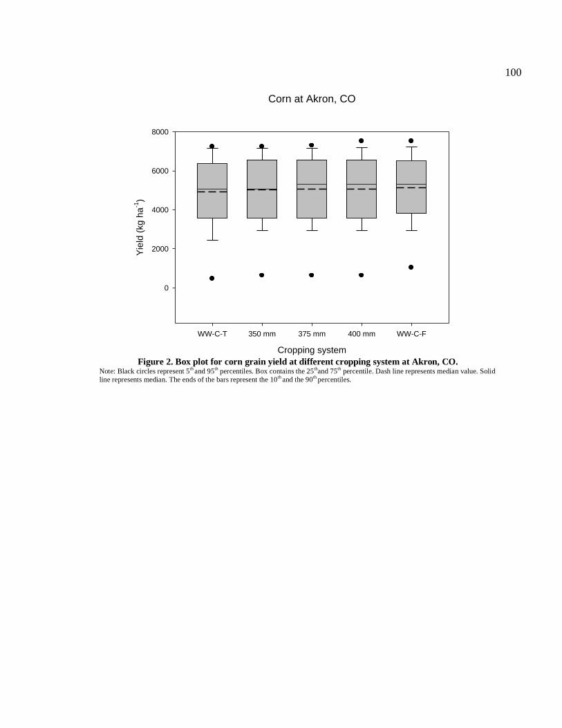
100

Corn at Akron, CO

Cropping system


Yie

ld (

kg

ha

-1)

0

2000

4000

6000

8000

Figure 2. Box plot for corn grain yield at different cropping system at Akron, CO.



thand 75



and the 90th

percentiles.

101

Triticale at Akron, CO

Cropping system

WW-C-T 350 mm 375 mm 400 mm

Yie

ld (

kg

ha

-1)

3600

3800

4000

4200

4400

4600

4800

5000

5200

5400

Figure 3. Box plot for triticale biomass yield at different cropping system at Akron, CO.



thand 75



and the 90th

percentiles.

102

Wheat at Sidney, NE

Cropping system


Yie

ld (

kg

ha

-1)

1200

1400

1600

1800

2000

2200

2400

2600

2800

3000

3200

Figure 4. Box plot for winter wheat grain yield at different cropping system at Sidney, NE.



thand 75



and the 90th

percentiles.

103

Corn at Sidney, NE

Cropping system


Yie

ld (

kg

ha

-1)

0

1000

2000

3000

4000

5000

6000

7000

8000

Figure 5. Box plot for corn grain yield at different cropping system at Sidney, NE.



thand 75



and the 90th

percentiles.

104

Triticale at Sidney, NE

Cropping system

WW-C-T 350 mm 375 mm 400 mm

Yie

ld (

kg

ha

-1)

4600

4800

5000

5200

5400

5600

5800

6000

6200

Figure 6. Box plot for triticale biomass yield at different cropping system at Sidney, NE.



thand 75



and the 90th

percentiles.

comparing cropping system productivity between fixed rotations

Documents