comparative analysis of mooring systems of floating
TRANSCRIPT
COMPARATIVE ANALYSIS OF MOORING SYSTEMS OF FLOATING CYLINDRICAL STRUCTURE IN TIME
DOMAIN
Vina Widya Lestari
Master Thesis
presented in partial fulfillment
of the requirements for the double degree: “Advanced Master in Naval Architecture” conferred by University of Liege
"Master of Sciences in Applied Mechanics, specialization in Hydrodynamics, Energetics and Propulsion” conferred by Ecole Centrale de Nantes
developed at University of Rostock
in the framework of the
“EMSHIP”
Erasmus Mundus Master Course in “Integrated Advanced Ship Design”
EMJMD 159652 – Grant Agreement 2015-1687
Supervisor:
Dipl.-Ing. Christoph Otto, University of Rostock
M.Sc. Stephan Schacht, University of Rostock
Reviewer: Prof. Mathias Paschen, University of Rostock
Prof. Philippe Rigo, University of Liege
Rostock, February 2018

ii
“EMSHIP” Erasmus Mundus Master Course, period of study September 2016 – February 2018
DECLARATION OF AUTHORSHIP
A signed declaration of authorship in the thesis must confirm that the
student personally wrote the whole text, all, figures, tables etc. are original,
excepted the cases a reference is clearly given. Violation of this rule will
result in rejecting the thesis and a grade of 0/20 for the thesis.
The following declaration should be added on a separate page after the table
of content.
Declaration of Authorship
I declare that this thesis and the work presented in it are my own and have
been generated by me as the result of my own original research.
Where I have consulted the published work of others, this is always clearly
attributed.
Where I have quoted from the work of others, the source is always given.
With the exception of such quotations, this thesis is entirely my own work.
I have acknowledged all main sources of help.
Where the thesis is based on work done by myself jointly with others, I have
made clear exactly what was done by others and what I have contributed
myself.
This thesis contains no material that has been submitted previously, in
whole or in part, for the award of any other academic degree or diploma.
I cede copyright of the thesis in favour of the University of …..
Date: Signature
iii
“EMSHIP” Erasmus Mundus Master Course, period of study September 2016 – February 2018
ABSTRACT
Mooring design has an essential influence on stability, seakeeping and
fatigue loads on offshore structures. It has thus become state of the art to
include detailed mooring analysis and optimisation as a crucial part of the
design process of moored systems. In this context it is common to carry
out large-scale time domain simulations for a number of well-defined
loadcases, which are usually defined by classification societies such as e.g.
DNV-GL. The analysis study will perform the comparison of different types
of mooring for an exemplary partially submerged cylindrical floating
structure.
The goal of analysis is to compare resulting loads in time domain using
a fully coupled dynamic analysis of the mooring and floater. The analysis is
using and extending approaches recently developed at the chair of ocean
engineering (OCN-SIM Flex Software, www.ocnacademy.org). In order to
facilitate a comparison, an extended hydrodynamic loads equation of the
floating structure is implemented and verified with mathematical model in
OCN-SIM Flex using the Airy wave theory with single unidirectional,
harmonic excitation. Dynamic tensioning or slackening by winches shall not
be considered. Moreover, the dynamic behaviour of the structure can be
characterized based on the results of the time-domain simulations. Thus,
for instance transfer functions can be determined by performing a frequency
analysis of the simulated time-domain response to harmonic wave
excitation.
iv
“EMSHIP” Erasmus Mundus Master Course, period of study September 2016 – February 2018
TABLE OF CONTENTS
DECLARATION OF AUTHORSHIP ii
ABSTRACT iii
TABLE OF CONTENTS iv
1. INTRODUCTION 1
1.1. Background 1
1.2. Objective of Research 3
1.3. Scope of Research 3
2. THEORETICAL BACKGROUND 5
2.1. Coordinate System and Equilibrium 5
2.1.1. Coordinate System 5
2.1.2. Stability and Equilibrium 6
2.2. Regular Wave – Linear Airy Wave 8
2.3. External Loads 14
2.3.1. Hydrodynamic Morison Force 16
2.3.2. Hydrostatic Force 17
2.3.3. Mooring Force 18
2.4. Coupled Dynamic Analysis 21
2.5. Motion and Response Analysis in Time Domain 23
3. ANALYSIS PROGRAMS 26
3.1. Langrangian Dynamics Methods 27
3.2. Reconstructed Reaction Forces Formulation Methods 30
4. HYDRODYNAMIC FORCES ON FLOATING CYLINDRICAL STRUCTURE AND
MOORING LINE 34
4.1. Implementation of Alghotythm in Matlab 34
4.1.1. Object Position and Velocity at Coordinate system 35
4.1.2. Wave Elevation 36
4.1.3. Airy Wave Velocity and Acceleration 37
4.1.4. Relative Velocity 38
v
“EMSHIP” Erasmus Mundus Master Course, period of study September 2016 – February 2018
4.1.5. Transformation of relative velocity, acceleration and filtering
result with respect to wave elevation 39
4.1.6. Added Mass and Drag Coefficient 40
4.1.7. Morison Equation 40
4.2. Plaussible Results 41
5. DESIGNED MODEL AND WAVE LOADCASES 46
5.1. Design Model of The Cylindrical Floating Structure 46
5.2. Mooring Configurations 47
5.3. Wave Loadcases 49
6. TIME DOMAIN ANALYSIS RESULT 51
6.1. Results and Comparison of Displacement Motion Response 51
6.2. Results and Comparison of Mooring Tensions Response 55
6.3. Results and Comparison of Stability 58
7. CONCLUSION AND FURTHER STUDIES 61
7.1. Conclusions 61
7.2. Further Studies 62
8. ACKNOWLEDGEMENTS 63
9. REFERENCES 64
APPENDIXES A. THE MOORING displacement and TENSION response
RESULT 66
APPENDIXES B. MATLAB CODES OF MORISON HYDRODYNAMIC LOAD
ALGORITHM for cylinder floating structure 70
APPENDIXES c. MATLAB CODES OF MORISON HYDRODYNAMIC LOAD
ALGORITHM for mooring line 78
APPENDIXES d. OCN SIM-FLEX INPUT CODES 86
1
“EMSHIP” Erasmus Mundus Master Course, period of study September 2016 – February 2018
1. INTRODUCTION
1.1. Background
Nowadays, a floating body structure with mooring system configuration
is being extensively used as an offshore facility not only in the oil/gas and
renewable energy industry, moreover, moorings of buoys are used in almost
every area of offshore engineering. This system has been deployed widely
around the world as a unique design facility which is regarded as a promising
concept for an flexibility and economic oil/gas and energy production. Floating
offshore structure, like any other, require stability to be operational especially
under extreme environmental conditions. Mooring systems are therefore
required to provide such stability againts structure dynamics, while ensuring
allowable excursion. With so much depending on the mooring systems of these
floating structures, it is worthwhile to understand the performance of each of
system components and the global reponse of the mooring system.
The nonlinear‐coupled dynamic analysis of the floating systems is
becoming more and more important in order to evaluate the dynamic
interaction among the floater and moorings. Concious of the fact that such
structures will be taken to ensure that their design are appreciably reliable.
One way to verify the analysis performed in the prototype design process is
by model testing. A model of design floater is built and subjected to the same
environmental loads in the wave basin as those used in the prototype design
with the deployed mooring system for stationkeeping. During testing, the
response and behaviour of the floater and mooring line system to various
forcing due to wind, wave and current are measured and compared to those
obtained in the design of the prototype floater. For as long as the testing
procedure is conceptually and practically correct, the result obtained
independently represent the performence to be expected of the prototype
floater under the given loading conditions, if it is installed in the field.
Conducting model tests requires wave basins, which are typically much
smaller than the prototype system, depending on the chosen model scale,

2
“EMSHIP” Erasmus Mundus Master Course, period of study September 2016 – February 2018
basin dimension may not be sufficiently large to accomodate the directly
scaled mooring system. Consequently, the size of the floater and the
accompanying mooring system are reduced such that they adequately fit into
the test facility, and the test engineer has a primary task to replicate the static
and dynamic behaviour of the prototype system on the model to be tested in
the wave basin. Essentially, the effects of the mooring system in the wave
basin on the model floater must be equal to those which the prototype
mooring system has on the full scale floater.
This introduce the need of such a program tools for evaluation of the
equivalent mooring system in order to represent it’s behaviour in the full depth
system. Lately, several software programs are established and developed in
order to perform the nonlinear‐coupled dynamic analysis of floating system,
such Orcaflex, Mimosa, ect. The use of those program tools mostly was costly
and not reachable by such student/reasercher. Therefore, OCN Simflex was
developed open-source, another motivation is to satisfy scientific needs, i.e.
be able to view and change the code depend on the needs. The program tools
project is under development process at the chair of ocean engineering
University of Rostock . At the mean time, the formulations that implemented
in the program are still focus mostly in mooring line, while for the
hydrodynamic calculation of the floating body still has to be implemented. This
introduces the need for the implementation of the floating structure
hydrodynamic force equations to the program tool, in order to process the
evaluation by the comparison analysis of the mooring systems and body
structure responses. In a later section of this report, a proper distinction of
the scope of work is drawn for clarity.
3
“EMSHIP” Erasmus Mundus Master Course, period of study September 2016 – February 2018
1.2. Objective of Research
The Mooring systems are major tools for maintaining the dynamic
responses of floating body . The challenge of understanding the behaviour of
a floating structure under environmental loads and influence of a mooring
system is quite hard, and the design of mooring system with high integrity
requires the ability to isolate the various dynamic effects induced by different
loads acting. The dynamic response of a floater combined with mooring
system would most often over-shadow its static response. For this reason, it
is considered good practice to study the mooring line behaviour and the
static/dynamic response of floater under its influence independently in design,
to allow a clear attribution of observed results to the correct floater responses.
In this study, the author presents a comparative study of mooring
systems analysis and develop a hydrodynamic loads algorithm by means of a
coupled time domain analysis and check the plausibility by means of simple
hard-coded examples in Matlab program. The algorithm is included a
numerically discrete implementation of drag term of morison equation.
Furthermore, The hydrodynamic loads algorithm will be used for the
implementation to the mooring analysis program tool (OCN Simflex,
www.ocnacademy.org), since at the mean time, the software program is in
development process and still need the implementation of floaters
hydrodynamic loads part. In order to execute the comparative analysis of
mooring systems, a response behaviour of both the mooring system and the
floater with considering non linear coupled dynamic analysis are presented.
The comparative analysis of response behaviour result are calculated fully in
time domain by simulating several case of mooring system configurations.
1.3. Scope of Research
The purpose of the research is to study the effect of mooring on a body
structure such a buoy. The analysis present a comparison analysis result of
4
“EMSHIP” Erasmus Mundus Master Course, period of study September 2016 – February 2018
several mooring systems configurations considering the non linear coupled
analysis. Generally, the study will cover the following activities below :
1. Establish, verify and test mathematically the hydrodynamic force
algorithm for a slender floater using Matlab Program.
2. Preparation of Floating cylinder structure main dimension, Mooring
Configuration and wave loadcases.
3. Evaluate the loadcases in time domain analysis and compare the result
concerning the response behaviour of mooring line and the floater.
Chapter 2 presents the theoretical background that will be helpful to give the
prespective for the analysis. The basic knowledge and key definitions that
relate to the analysis will be present here.
Chapter 3 presents the overall description of the software programs that is
used in the analysis, the analysis use two program, OCN Simflex and Matlab.
Chapter 4 presents the implementation of hydrodynamic force algorithm
steps for a floater, which is modelled as a slender cylindrical structure using
Matlab program.
Chapter 5 presents the main dimension preparation of the cylindrical floating
structure and mooring system configurations, the loadcases scenario, and
finally the evaluation procedure in time domain.
Chapter 6 presents the comparative result of the loadcases evaluation in time
domain analysis concerning the loads, seakeeping, mooring/floaters response
behaviour and stability with single harmonic excitation using OCN Simflex
program. Furthermore, comparing the result of each configurations of mooring
system.
Chapter 7 provides the conclusions and the recommended further studies
from this study.
5
“EMSHIP” Erasmus Mundus Master Course, period of study September 2016 – February 2018
2. THEORETICAL BACKGROUND
This chapter will review the basic knowledge to give a perspective for the
analysis. Furthermore the key definitions that are related to the analysis will
also be explained here. The explanations are separated in several part
regarding the subsequents of the calculation procedure as follows :
1. Coordinate System and Equilibrium
2. Regular Wave - Linear Airy Wave
3. External Loads
4. Coupled Dynamic Analysis
5. Motion and Response Analysis (in time domain)
The Hydrodynamic Loads, in Point 2 is described generally in this chapter,
while for the detail explanation is provided in chapter 4.
2.1. Coordinate System and Equilibrium
2.1.1. Coordinate System
There will be two systems of orthogonal that used, in order to express
and resolve the various vectors of the model. The global system serves as an
absolute, earth-fixed reference of the cylinder body position and orientation.
The local system serves the body bound reference of cylinder body position
and orientation. Cylinder body is assumed as unconstrained due to force-
based coupling of rigid bodies to the mooring in OCN-Simflex. The Cylinder
body is defined in the global coordinate system correspond to 6 degree of
freedom which expressed as coordinate direction. The 6 coordinates consist
of 3 coordinates of body translation at (x, y, and z) axes and 3 coordinates of
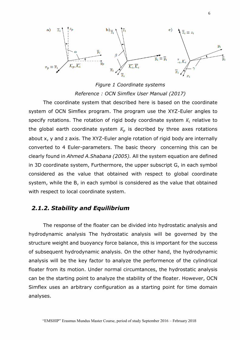
body orientation that rotate about the axes. Furthermore, the first angular
displacement of body orientation 𝛼 about x axis is the pitch, the second
angular displacement of body orientation 𝛽 about y axis is the roll and the
third angular displacement of body orientation 𝛾 about z axis is the yaw. The
global and local coordinate system are shown as follows :
6
“EMSHIP” Erasmus Mundus Master Course, period of study September 2016 – February 2018
Figure 1 Coordinate systems
Reference : OCN Simflex User Manual (2017)
The coordinate system that described here is based on the coordinate
system of OCN Simflex program. The program use the XYZ-Euler angles to
specify rotations. The rotation of rigid body coordinate system 𝐾𝑖 relative to
the global earth coordinate system 𝐾𝑝 is decribed by three axes rotations
about x, y and z axis. The XYZ-Euler angle rotation of rigid body are internally
converted to 4 Euler-parameters. The basic theory concerning this can be
clearly found in Ahmed A.Shabana (2005). All the system equation are defined
in 3D coordinate system, Furthermore, the upper subscript G, in each symbol
considered as the value that obtained with respect to global coordinate
system, while the B, in each symbol is considered as the value that obtained
with respect to local coordinate system.
2.1.2. Stability and Equilibrium
The response of the floater can be divided into hydrostatic analysis and
hydrodynamic analysis The hydrostatic analysis will be governed by the
structure weight and buoyancy force balance, this is important for the success
of subsequent hydrodynamic analysis. On the other hand, the hydrodynamic
analysis will be the key factor to analyze the performence of the cylindrical
floater from its motion. Under normal circumtances, the hydrostatic analysis
can be the starting point to analyze the stability of the floater. However, OCN
Simflex uses an arbitrary configuration as a starting point for time domain
analyses.
7
“EMSHIP” Erasmus Mundus Master Course, period of study September 2016 – February 2018
Stability analysis describes the position of the floater in static
equilibrium where the forces of gravity and buoyancy are equal and acting in
opposite directions in line with one another. Ship Hydrostatic (2002) has
mentioned that stability is the ability of a body, in this setting a ship or floating
vessel, to resist the overturning forces and return to its original position after
the disturbing forces are removed, It requires initial stability. Initial stability
is achieved from a small perturbation from its original position. There will be
initial stability when there is an uprighting moment larger than zero. Hence,
the floater will be back to its initial position when the inclining moment is taken
away.
Based on Newton’s law, Journee,J.M.J (2001), explain that a floating
structureis said to be in a state of equilibrium or balance when the resultat of
all the forces acting on it is zero and the resulting moment of these forces is
also zero. If a structure is floating freely in rest in fluid, the following
equilibrium or balance condition are fulfilled :
Horizontal equilibrium, the sum of the horizontal forces equal to
zero, may influenced by other external force such moorings
Vertical equilibrium, the sum of the vertical forces equal to zero,
using Archimides principle which hold for the vertical equilibrium
between buoyancy and gravity forces as follows :
𝜌𝑔∇= 𝑔𝑚 (2.4)
Then derive to the change of draft ΔT which caused by additional
mass, p :
∆𝑇 =𝑝
𝜌.𝐴𝑊𝐿 (2.5)
∆𝑇 = change of draft due to additional mass
𝑝 = additional mass
𝜌 = water density
𝐴𝑊𝐿 = water plane area
g = gravity acceleration
∇ = Volume of the submerged body
m = mass/weight of body
8
“EMSHIP” Erasmus Mundus Master Course, period of study September 2016 – February 2018
Rotational equilibrium, the sum of the moments about G – or any
other point equals to zero, with rotational equilibrium equation as
present below (when an external heeling moment acts on the
structure) :
𝑀𝐻 = 𝜌𝑔∇. 𝑦 = 𝑔𝑚. 𝑦 (2.6)
Where y is lever arm.
2.2. Regular Wave – Linear Airy Wave
The study will analyze the wave loads by using regular waves form, in
order to calculate the loads on cylindrical floater. The classical linear wave
theory developed by Airy and Laplace will be used. Chakrabarti,S.[2005] has
described that regular waves have the characteritics of periodic process which
the surface elevation has the shape of harmonic function. Hence, the theory
will describe the properties of one cycle in regular waves and these properties
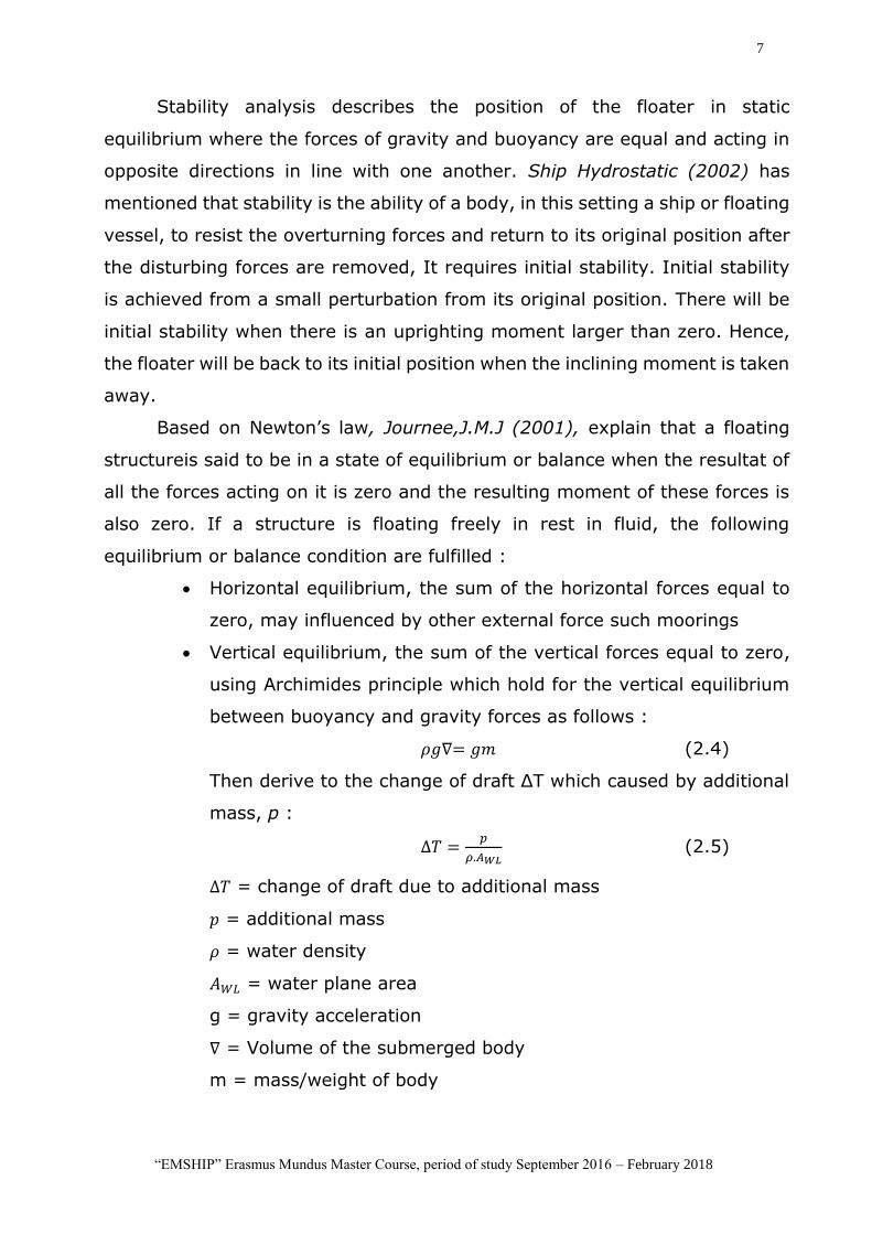
are invariant from cycle to cycle. Below figure show a harmonic wave seen
from two different perspectives, the wave profile that shown as a function of
distance x at a fixed instant in time, and as function of time record of water
level observed at one location.
Figure 2 Harmonic wave definition.
Reference:Journee and Massie (2001)
The x axis is positive in the direction of wave propagation, the still water
level is the average water level when there is not wave is present. The z axis
is directed upward with positive value, most of relevant values of z are
negative which are below the water level. The water depth, h with positive
value is distance between the seabed and still water level (z = -d). The
horizontal distance (measured in direction of wave propagation) between any
9
“EMSHIP” Erasmus Mundus Master Course, period of study September 2016 – February 2018
two successive wave crest along x axis in space domain is the wave length, λ.
The distance between any two successive wave crest along time domain is
the wave period, T.
The potential theory is used to solve the flow problem in regular waves.
In order to use this linear wave theory, it will be necessary to assume that the
water surface slope is very small, this means that the wave steepness is so
small. Hence, the terms in the equations of the waves with a magnitude in the
order of the steepness-squared can be ignored. Using the linear theory holds
here that harmonic displacements, velocities and accelerations of the water
particles and also the harmonic pressures will have a linear relation with
respect to the wave surface elevation.
A velocity potential φ can be used to describe the velocity field at time t. The
velocity of water particles (u,v,w) in three translational direction follow from
the definition of velocity potential φ :
𝑢 =𝜕φ
𝜕𝑥, 𝑣 =
𝜕φ
𝜕𝑦, 𝑤 =
𝜕φ
𝜕𝑦
�⃗⃗� = (𝑢, 𝑣, 𝑤) = (𝜕φ
𝜕𝑥.𝜕φ
𝜕𝑦.𝜕φ
𝜕𝑧) (2.7)
∇𝜑= �⃗⃗� =𝜕φ
𝜕𝑥 . 𝑖 ,⃗⃗
𝜕φ
𝜕𝑦 . 𝑗 ,⃗⃗⃗
𝜕φ
𝜕𝑧 . �⃗�
Where,
𝑢, 𝑣, 𝑤 = velocities of water particle at x, y and z axis direction
𝜕φ
𝜕𝑥.𝜕φ
𝜕𝑦.𝜕φ
𝜕𝑧 = partial derivatives of the velocities at x, y and z axis direction
∇𝜑 = gradient of scalar function / velocity potential
The profile of simple wave with small steepness style has the shape of sine or
cosine and the motion of water particle in a wave depend on water depth and
wave phase.
𝜑(𝑥, 𝑧, 𝑡) = 𝑃(𝑧) . sin (𝑘𝑥 − 𝑤𝑡) (2.8)
Which p(z) is (as yet) an unknown function of z. The velocity potential φ(x,z,t)
of the harmonic waves has to fulfill requrements as follows :
1. Continuity condition or Laplace equation
There are two important assumptions in order to arrive to Laplace
equation, First assumptions is continuity equation for homogeneous and
incompressible flow :
10
“EMSHIP” Erasmus Mundus Master Course, period of study September 2016 – February 2018
∇𝑥�⃗⃗� =𝜕u
𝜕𝑥+𝜕v
𝜕𝑦+𝜕w
𝜕𝑧= 0 (2.9)
Where,
∇ = 𝜕
𝜕𝑥,𝜕
𝜕𝑦,𝜕
𝜕𝑧 = nabla operator
�⃗⃗� = velocity vector
Second asssumption is Non rotational/invicid flow. Concequently, the
motion is irrotational if the rotation vector or vorticity, 𝜔𝑣 is zero, i.e.
𝜔𝑣 = ∇𝑥�⃗⃗� = |
𝑖 ⃗ 𝑗 ⃗⃗ 𝑘 ⃗⃗⃗
𝜕φ
𝜕𝑥
𝜕φ
𝜕𝑦
𝜕φ
𝜕𝑧
𝑢 𝑣 𝑤
| = 𝑖 ⃗ (𝜕w
𝜕𝑦−𝜕v
𝜕𝑧) − 𝑗 ⃗⃗ (
𝜕w
𝜕𝑥−𝜕u
𝜕𝑧) + 𝑘 ⃗⃗⃗ (
𝜕v
𝜕𝑥−𝜕u
𝜕𝑦) = 0 ⃗⃗⃗
(2.10)
By using two assumption above, we will find the Laplace equation:
∇2φ =𝜕2φ
𝜕𝑥2+𝜕2φ
𝜕𝑦2+𝜕2φ
𝜕𝑧2= 0 (2.11)
Subtituting equation 2.8 into 2.11 we get P(z) and wave potential :
𝑑2P(z)
𝜕𝑧2− 𝑘2𝑃(𝑧) = 0 → 𝑃(𝑧) = 𝐶1𝑒
+𝑘𝑧 + 𝐶2𝑒−𝑘𝑧 (2.12)
𝜑(𝑥, 𝑧, 𝑡) = (𝐶1𝑒+𝑘𝑧 + 𝐶2𝑒
−𝑘𝑧) . sin (𝑘𝑥 − 𝑤𝑡) (2.13)
Where C1 and C2 as yet undetermined constants. The complete
mathematical problem in order to find a velocity potential of Non
rotational and incompressible fluid motion consist of the solution of the
Laplace equation with respect to relevant boundary condition in the
fluid. The boundary conditions will be found from physical
considerations.
2. Boundary Conditions
a. Bottom Condition
No water can flow through the bottom, a flat bottom will be
considered here.
𝑤|𝑧=−𝑑 = 0 → 𝜕φ
𝜕𝑧|𝑧=−𝑑
= 0 (2.14)
Where d is the water depth. Subtituting boundary condition into
equation 2.13 we get P(z) and wave potential :
𝐶1 =𝐶
2𝑒+𝑘𝑑 , 𝐶2 =
𝐶
2𝑒−𝑘𝑑 → 𝑃(𝑧) =
𝐶
2(𝑒+𝑘(𝑑+𝑧) + 𝑒−𝑘(𝑑+𝑧)) = 𝐶 cosh 𝑘(𝑑 + 𝑧) (2.15)
𝜑(𝑥, 𝑧, 𝑡) = 𝐶 cosh 𝑘(𝑑 + 𝑧) . sin (𝑘𝑥 − 𝑤𝑡) (2.16)
Where C as yet undetermined constant.
11
“EMSHIP” Erasmus Mundus Master Course, period of study September 2016 – February 2018
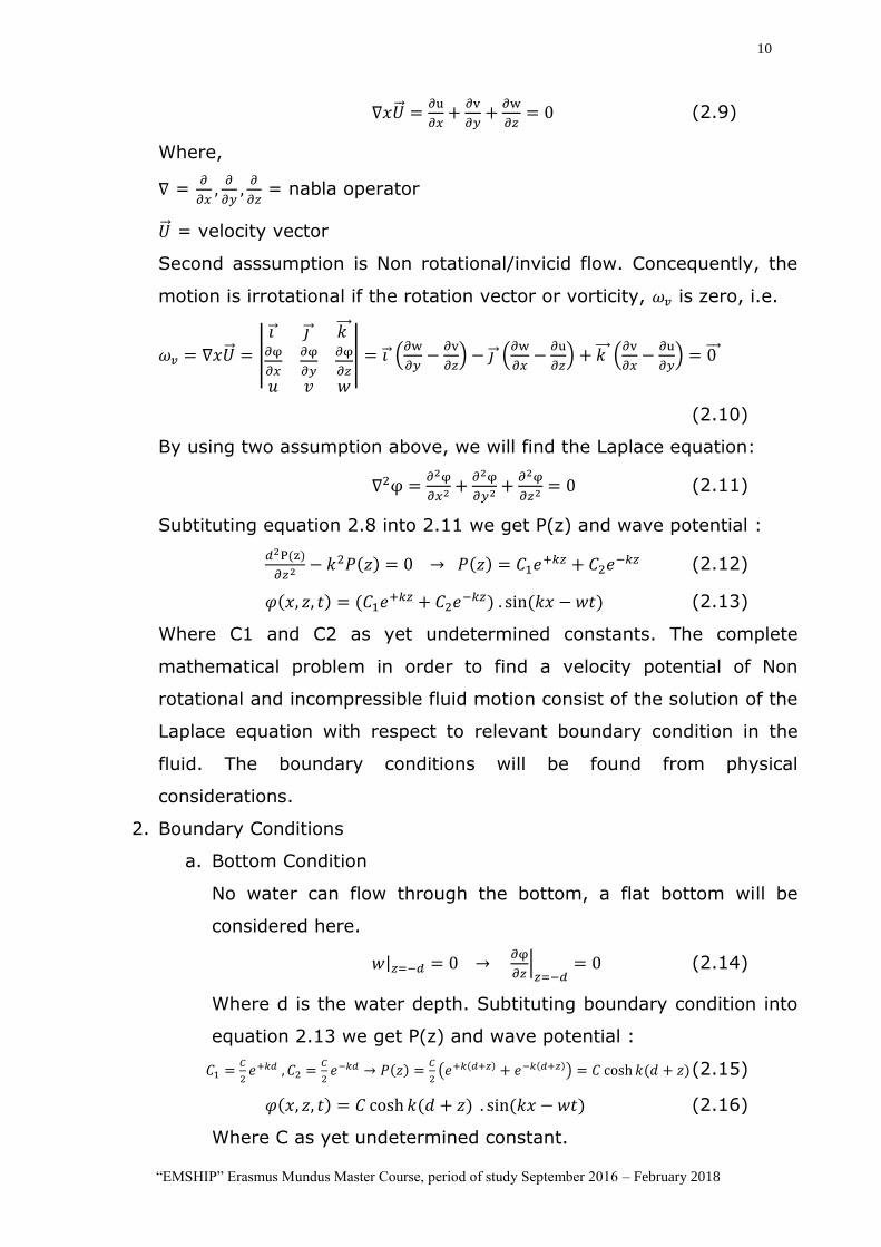
b. Surface condition
The distinction between the different type of fluid motion result
come from the condition of the boundaries which is imposed on
the fluid domain. Two types of surface boundary conditions will be
considered :
Free Surface Dynamic Boundary Condition
This criterion is corresponding with the forces on the boundary.
At the free surface, boundary condition is simply that, the
water pressure is equal to constant atmospheric pressure, p0
on the free surface.
Figure 3 Atmospheric pressure at the free surface
Reference:Journee and Massie (2001)
The Bernoulli equation for an unstationary irrotational flow :
𝑃
𝜌+ 𝑔 . 𝑧 +
𝜕φ
𝜕𝑧+1
2(𝑢2 + 𝑤2) = 𝐶𝑡 (2.17)
At surface P = 𝑃0 and 𝑧 = 𝜉(𝑥, 𝑡) ∶
𝑔 . 𝜉 +𝜕φ
𝜕𝑡|𝑧=𝜉
+1
2(𝑢2 + 𝑤2)|𝑧=𝜉 = 0 (2.18)
Since we still use assumption that the water slope is very small
which means that the convective velocity term also become
small, linearizing can be applied. Hence, 1
2(𝑢2 + 𝑤2)|𝑧=𝜉 = 0 can
be neglected. And we apply the boundary z = ξ → 𝑧 = 0 and
yields :
𝜕φ
𝜕𝑡|𝑧=𝜉
=𝜕φ
𝜕𝑡|𝑧=0
(2.19)
Hence, the equation 2.21 at the surface can be written as
follows :
𝑔 . 𝜉 +𝜕φ
𝜕𝑡|𝑧=0
= 0 → 𝜉 = −1
𝑔 .𝜕φ
𝜕𝑡|𝑧=0
(2.20)
d
12
“EMSHIP” Erasmus Mundus Master Course, period of study September 2016 – February 2018
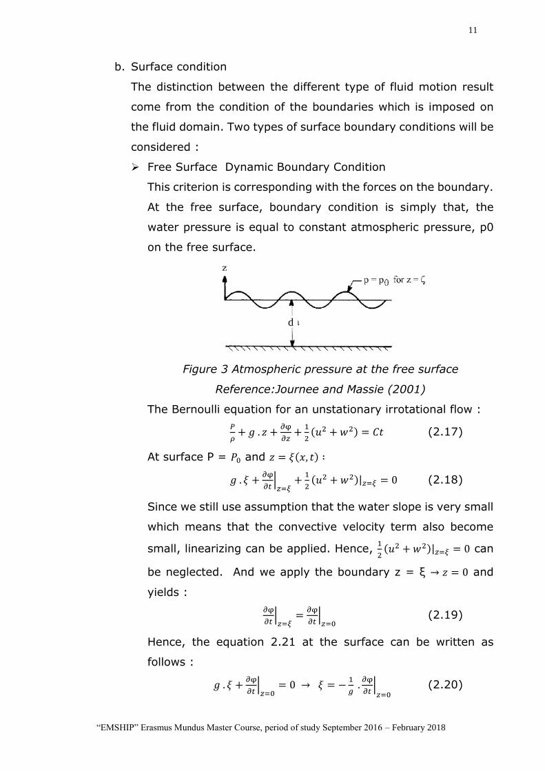
Subtituting equation 2.16 into 2.20 we get wave profile and
wave potential:
𝜉 = 𝜉𝑎 . cos(𝑘𝑥 − 𝜔𝑡) 𝑤𝑖𝑡ℎ 𝜉𝑎 =𝜔𝐶
𝑔 . cosh 𝑘ℎ (2.21)
φ =𝜉𝑎𝑔
𝜔 .cosh𝑘(𝑑+𝑧)
cosh𝑘𝑑 . sin (𝑘𝑥 − 𝜔𝑡) (2.22)
Figure 4 Sinusoidal wave profile
Reference : Gudmestad(2010)
Free Surface Kinematic Boundary Condition
A water particle at free surface will always remain at surface.
Let’s consider the velocity in the vertical direction as :
𝑤 =𝜕φ
𝜕𝑧=𝐷𝑧
𝐷𝑡|𝑧=𝜉(𝑥,𝑡)
= (𝜕z
𝜕𝑡+ 𝑢 .
𝜕z
𝜕𝑥 )|𝑧=𝜉(𝑥,𝑡)
= (𝜕𝜉
𝜕𝑡+ 𝑢 .
𝜕𝜉
𝜕𝑥 ) (2.23)
Since we use the water surface slope is very small which means
that the wave steepness is also small, hence, a linearizing can
be applied and leads :
𝜕φ
𝜕𝑧|𝑧=𝜉(𝑥,𝑡))
=𝜕φ
𝜕𝑧|𝑧=0
= 𝜕𝜉
𝜕𝑡 (2.24)
Here, the non-linear cross term 𝑢𝜕𝜉
𝜕𝑡 term becomes smaller
(second order) and can be disregarded. And the velocity at
wave surface is set equal to the velocity at still surface. A
differentiation of the free surface boundary condition equation
2.20 with respect to t yields :
𝜕2φ
𝜕𝑡2+ 𝑔
𝜕𝜉
𝜕𝑡= 0 →
𝜕𝜉
𝜕𝑡+1
𝑔 .𝜕2φ
𝜕𝑡2= 0 𝑓𝑜𝑟 𝑧 = 0 (2.25)
Combining equation 2.27 and 2.28 delivers the free surface
kinematic boundary condition called Cauchy-Poisson condition:
Velocity at
still surface
Velocity at wave
surface
13
“EMSHIP” Erasmus Mundus Master Course, period of study September 2016 – February 2018
𝜕𝑧
𝜕𝑡+1
𝑔 .𝜕2φ
𝜕𝑡2= 0 𝑓𝑜𝑟 𝑧 = 0 (2.26)
In order to obtain the final linear flow velocity, we need to establish the
relationship between ω and k (or equivalently T and 𝜆) referred to above. A
subtitution of wave potential equation 2.22 into 2.26 gives dispersion relation
for arbitrary water depth d.
𝜔2 = 𝑘 𝑔 . tanh 𝑘ℎ (2.27)
Hence, by combining velocity potential equation 2.22 and dispersion relation
equation 2.27, we obtain kinematic of water particle flow velocity in x (u) and
z (w) directions as water particle kinematics:
𝑢 = 𝜉𝑎 . 𝜔 .cosh𝑘(𝑑+𝑧)
sinh𝑘𝑑 . cos(𝑘𝑥 − 𝜔𝑡) (2.28)
𝑤 = 𝜉𝑎 . 𝜔 .sinh𝑘(𝑑+𝑧)
sinh𝑘𝑑 . sin(𝑘𝑥 − 𝜔𝑡)
While, the acceleration are definned as derivation of flow velocity and
written as follows :
�̇� = 𝜉𝑎. 𝜔2.cosh𝑘(𝑑+𝑧)
sinh𝑘𝑑. sin (𝑘𝑥 − 𝜔𝑡) (2.29)
�̇� = −𝜉𝑎. 𝜔2.sinh 𝑘(𝑑 + 𝑧)
sinh 𝑘𝑑. cos (𝑘𝑥 − 𝜔𝑡)
14
“EMSHIP” Erasmus Mundus Master Course, period of study September 2016 – February 2018
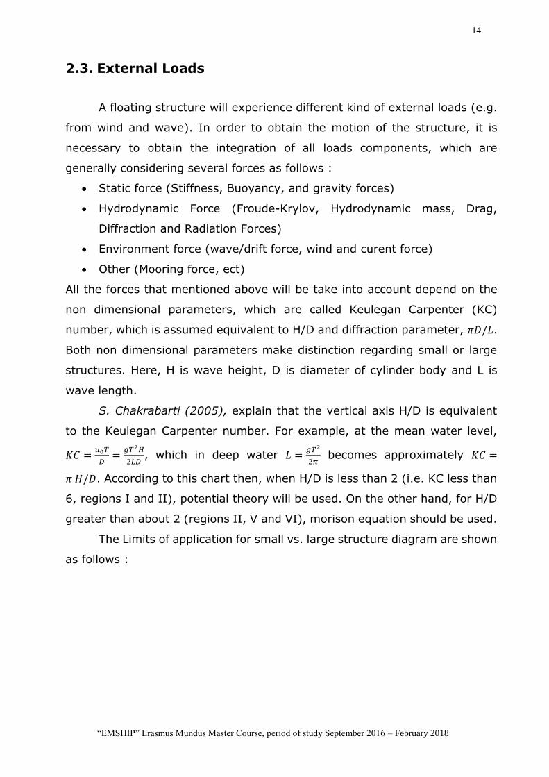
2.3. External Loads
A floating structure will experience different kind of external loads (e.g.
from wind and wave). In order to obtain the motion of the structure, it is
necessary to obtain the integration of all loads components, which are
generally considering several forces as follows :
Static force (Stiffness, Buoyancy, and gravity forces)
Hydrodynamic Force (Froude-Krylov, Hydrodynamic mass, Drag,
Diffraction and Radiation Forces)
Environment force (wave/drift force, wind and curent force)
Other (Mooring force, ect)
All the forces that mentioned above will be take into account depend on the
non dimensional parameters, which are called Keulegan Carpenter (KC)
number, which is assumed equivalent to H/D and diffraction parameter, 𝜋𝐷/𝐿.
Both non dimensional parameters make distinction regarding small or large
structures. Here, H is wave height, D is diameter of cylinder body and L is
wave length.
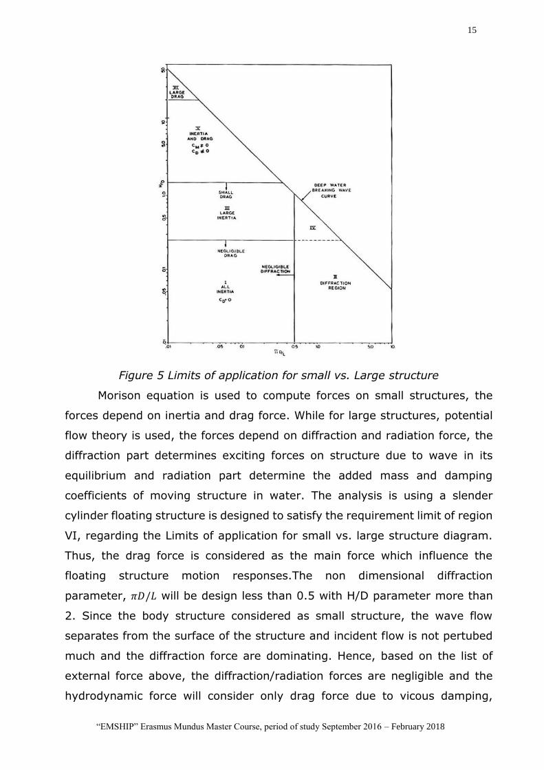
S. Chakrabarti (2005), explain that the vertical axis H/D is equivalent
to the Keulegan Carpenter number. For example, at the mean water level,
𝐾𝐶 =𝑢0𝑇
𝐷=𝑔𝑇2𝐻
2𝐿𝐷, which in deep water 𝐿 =
𝑔𝑇2
2𝜋 becomes approximately 𝐾𝐶 =
𝜋 𝐻/𝐷. According to this chart then, when H/D is less than 2 (i.e. KC less than
6, regions I and II), potential theory will be used. On the other hand, for H/D
greater than about 2 (regions II, V and VI), morison equation should be used.
The Limits of application for small vs. large structure diagram are shown
as follows :
15
“EMSHIP” Erasmus Mundus Master Course, period of study September 2016 – February 2018
Figure 5 Limits of application for small vs. Large structure
Morison equation is used to compute forces on small structures, the
forces depend on inertia and drag force. While for large structures, potential
flow theory is used, the forces depend on diffraction and radiation force, the
diffraction part determines exciting forces on structure due to wave in its
equilibrium and radiation part determine the added mass and damping
coefficients of moving structure in water. The analysis is using a slender
cylinder floating structure is designed to satisfy the requirement limit of region
VI, regarding the Limits of application for small vs. large structure diagram.
Thus, the drag force is considered as the main force which influence the
floating structure motion responses.The non dimensional diffraction
parameter, 𝜋𝐷/𝐿 will be design less than 0.5 with H/D parameter more than
2. Since the body structure considered as small structure, the wave flow
separates from the surface of the structure and incident flow is not pertubed
much and the diffraction force are dominating. Hence, based on the list of
external force above, the diffraction/radiation forces are negligible and the
hydrodynamic force will consider only drag force due to vicous damping,
16
“EMSHIP” Erasmus Mundus Master Course, period of study September 2016 – February 2018
friction force will be neglected since the analysis concern to floating body
motions not for body structure resistance analysis. For other external load,
such mooring force is considered also since the body structure will have
interaction with a mooring system configuration. In this analysis the static
force will be combination of buoyancy and gravity force only without stiffness.
As summation, in this analysis. All force components are neglected,except the
drag force, buoyancy and gravity force.
2.3.1. Hydrodynamic Morison Force
As already mentioned previously that the body structure in the analysis
is assumed as slender (hydrodynamically transparent) structure, since
diffraction and reflection phenomena are negligible. Hence, The hydrodynamic
equation is determined by using morison equation method. In order to
calculate hydrodynamic forces, it is necessary to integrate pressure field over
the wetted surface. The main force components are :
Froude Krylov load, follows from the pressure field of the
undisturbed wave (froude-krylov term)
Load due to added mass, follows from the pressure field of relative
acceleration of fluid and structure (hydrodynamic mass term)
Load due to viscosity, follows from the pressure field of relative
velocity of fluid and structure (non linear drag term)
Morison et al proposed as approach in which the horizontal and vertical force
on a section of body structure is express as sum of an inertia force and non
linear drag force. For a fixed cylinder structure in the wave flow, the linear
inertia force resulting from froude krylov and hydrodynamic mass force, while
non linear drag is caused by viscous effect and the associated downstream
wake. The viscous force includes form and friction drag, and it is proportional
to the drag coefficient, 𝐶𝑑, as well as to the square of the instationary flow
velocity, where the notation |𝑢|𝑢 ensures that drag force and velocity always
always act in the same direction. Both of forces yield a hydrodynamic forces
in a flow direction as follows :
17
“EMSHIP” Erasmus Mundus Master Course, period of study September 2016 – February 2018
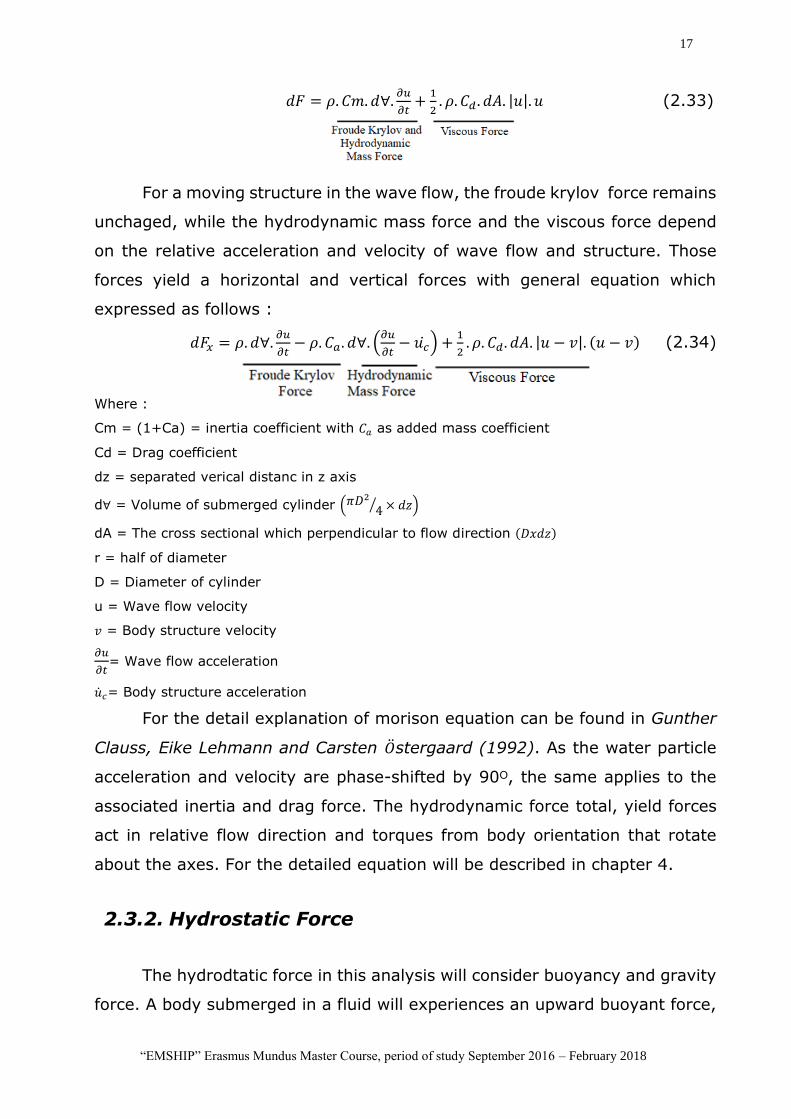
𝑑𝐹 = 𝜌. 𝐶𝑚. 𝑑∀.𝜕𝑢
𝜕𝑡+1
2. 𝜌. 𝐶𝑑 . 𝑑𝐴. |𝑢|. 𝑢 (2.33)
For a moving structure in the wave flow, the froude krylov force remains
unchaged, while the hydrodynamic mass force and the viscous force depend
on the relative acceleration and velocity of wave flow and structure. Those
forces yield a horizontal and vertical forces with general equation which
expressed as follows :
𝑑𝐹𝑥 = 𝜌. 𝑑∀.𝜕𝑢
𝜕𝑡− 𝜌. 𝐶𝑎. 𝑑∀. (
𝜕𝑢
𝜕𝑡− 𝑢�̇�) +
1
2. 𝜌. 𝐶𝑑. 𝑑𝐴. |𝑢 − 𝑣|. (𝑢 − 𝑣) (2.34)
Where :
Cm = (1+Ca) = inertia coefficient with 𝐶𝑎 as added mass coefficient
Cd = Drag coefficient
dz = separated verical distanc in z axis
d∀ = Volume of submerged cylinder (𝜋𝐷2
4⁄ × 𝑑𝑧)
dA = The cross sectional which perpendicular to flow direction (𝐷𝑥𝑑𝑧)
r = half of diameter
D = Diameter of cylinder
u = Wave flow velocity
𝑣 = Body structure velocity
𝜕𝑢
𝜕𝑡= Wave flow acceleration
�̇�𝑐= Body structure acceleration
For the detail explanation of morison equation can be found in Gunther
Clauss, Eike Lehmann and Carsten �̈�stergaard (1992). As the water particle
acceleration and velocity are phase-shifted by 90ᴼ, the same applies to the
associated inertia and drag force. The hydrodynamic force total, yield forces
act in relative flow direction and torques from body orientation that rotate
about the axes. For the detailed equation will be described in chapter 4.
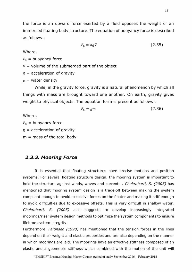
2.3.2. Hydrostatic Force
The hydrodtatic force in this analysis will consider buoyancy and gravity
force. A body submerged in a fluid will experiences an upward buoyant force,
18
“EMSHIP” Erasmus Mundus Master Course, period of study September 2016 – February 2018
the force is an upward force exerted by a fluid opposes the weight of an
immersed floating body structure. The equation of buoyancy force is described
as follows :
𝐹b = 𝜌𝑔∇ (2.35)
Where,
𝐹b = buoyancy force
∇ = volume of the submerged part of the object
g = acceleration of gravity
𝜌 = water density
While, in the gravity force, gravity is a natural phenomenon by which all
things with mass are brought toward one another. On earth, gravity gives
weight to physical objects. The equation form is present as follows :
𝐹𝐺 = 𝑔𝑚 (2.36)
Where,
𝐹G = buoyancy force
g = acceleration of gravity
m = mass of the total body
2.3.3. Mooring Force
It is essential that floating structures have precise motions and position
systems. For several floating structure design, the mooring system is important to
hold the structure against winds, waves and currents . Chakrabarti, S. (2005) has
mentioned that mooring system design is a trade‐off between making the system
compliant enough to avoid excessive forces on the floater and making it stiff enough
to avoid difficulties due to excessive offsets. This is very difficult in shallow water.
Chakrabarti, S. (2005) also suggests to develop increasingly integrated
moorings/riser system design methods to optimize the system components to ensure
lifetime system integrity.
Furthermore, Faltinsen (1990) has mentioned that the tension forces in the lines
depend on their weight and elastic properties and are also depending on the manner
in which moorings are laid. The moorings have an effective stiffness composed of an
elastic and a geometric stiffness which combined with the motion of the unit will
19
“EMSHIP” Erasmus Mundus Master Course, period of study September 2016 – February 2018
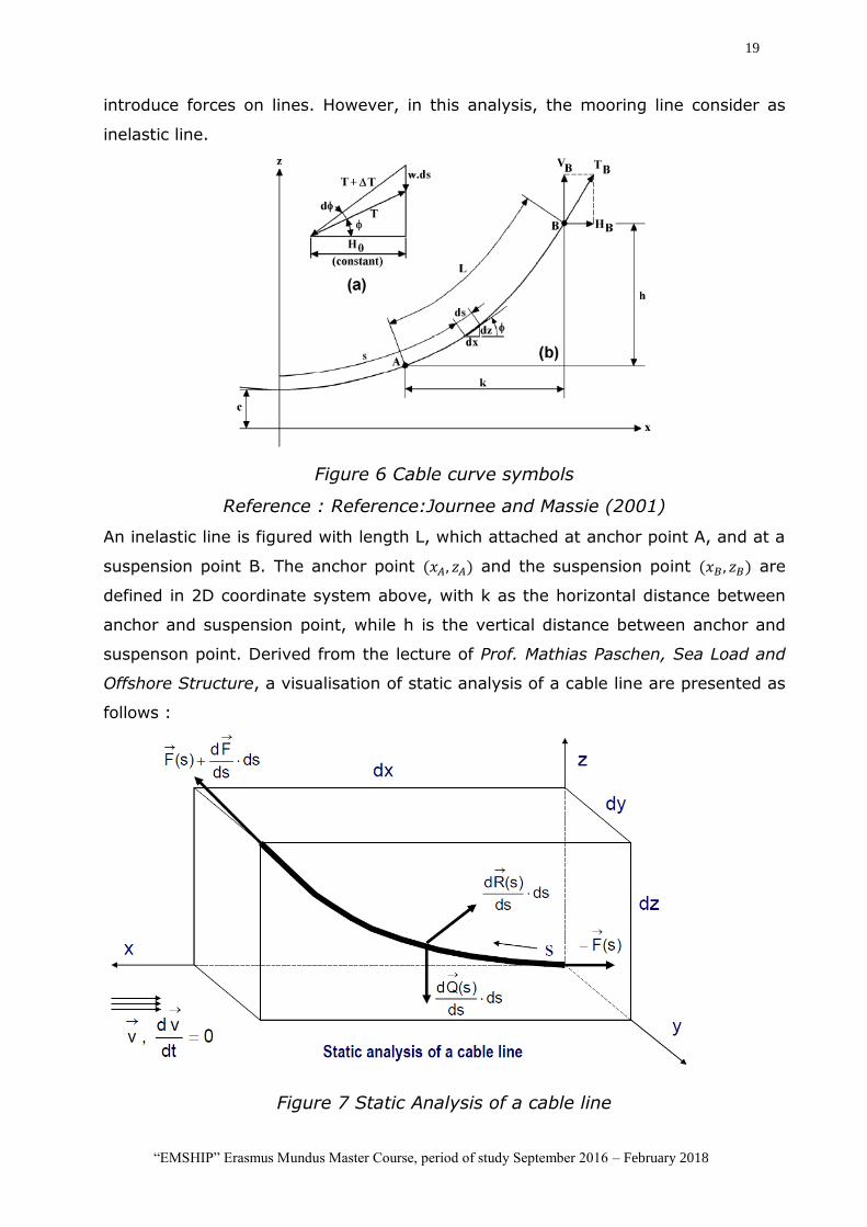
introduce forces on lines. However, in this analysis, the mooring line consider as
inelastic line.
Figure 6 Cable curve symbols
Reference : Reference:Journee and Massie (2001)
An inelastic line is figured with length L, which attached at anchor point A, and at a
suspension point B. The anchor point (𝑥𝐴, 𝑧𝐴) and the suspension point (𝑥𝐵, 𝑧𝐵) are
defined in 2D coordinate system above, with k as the horizontal distance between
anchor and suspension point, while h is the vertical distance between anchor and
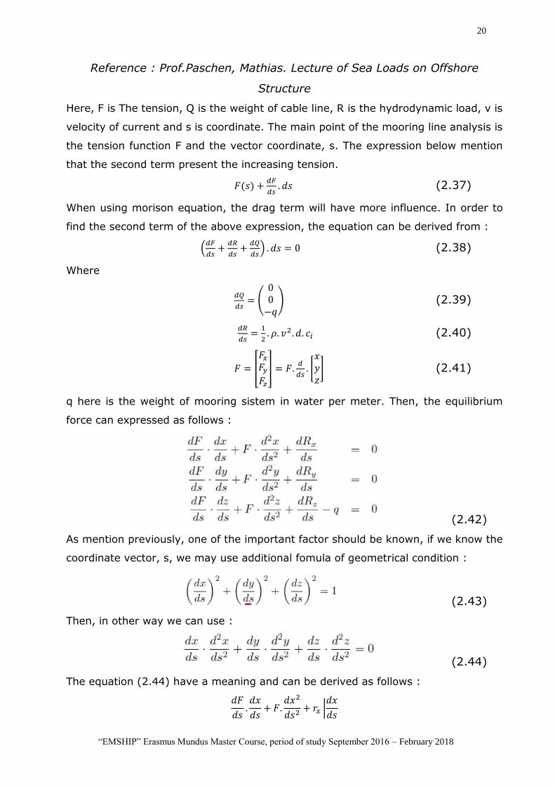
suspenson point. Derived from the lecture of Prof. Mathias Paschen, Sea Load and
Offshore Structure, a visualisation of static analysis of a cable line are presented as
follows :
Figure 7 Static Analysis of a cable line
20
“EMSHIP” Erasmus Mundus Master Course, period of study September 2016 – February 2018
Reference : Prof.Paschen, Mathias. Lecture of Sea Loads on Offshore
Structure
Here, F is The tension, Q is the weight of cable line, R is the hydrodynamic load, v is
velocity of current and s is coordinate. The main point of the mooring line analysis is
the tension function F and the vector coordinate, s. The expression below mention
that the second term present the increasing tension.
𝐹(𝑠) +𝑑𝐹
𝑑𝑠. 𝑑𝑠 (2.37)
When using morison equation, the drag term will have more influence. In order to
find the second term of the above expression, the equation can be derived from :
(𝑑𝐹
𝑑𝑠+𝑑𝑅
𝑑𝑠+𝑑𝑄
𝑑𝑠) . 𝑑𝑠 = 0 (2.38)
Where
𝑑𝑄
𝑑𝑠= (
00−𝑞) (2.39)
𝑑𝑅
𝑑𝑠=1
2. 𝜌. 𝑣2. 𝑑. 𝑐𝑖 (2.40)
𝐹 = [
𝐹𝑥𝐹𝑦𝐹𝑧
] = 𝐹.𝑑
𝑑𝑠. [𝑥𝑦𝑧] (2.41)
q here is the weight of mooring sistem in water per meter. Then, the equilibrium
force can expressed as follows :
(2.42)
As mention previously, one of the important factor should be known, if we know the
coordinate vector, s, we may use additional fomula of geometrical condition :
(2.43)
Then, in other way we can use :
(2.44)
The equation (2.44) have a meaning and can be derived as follows :
𝑑𝐹
𝑑𝑠.𝑑𝑥
𝑑𝑠+ 𝐹.
𝑑𝑥2
𝑑𝑠2+ 𝑟𝑥 |
𝑑𝑥
𝑑𝑠
21
“EMSHIP” Erasmus Mundus Master Course, period of study September 2016 – February 2018
𝑑𝐹
𝑑𝑠.𝑑𝑦
𝑑𝑠+ 𝐹.
𝑑𝑦2
𝑑𝑠2+ 𝑟𝑦 |
𝑑𝑥
𝑑𝑠
𝑑𝐹
𝑑𝑠.𝑑𝑧
𝑑𝑠+ 𝐹.
𝑑𝑧2
𝑑𝑠2+ 𝑟𝑧 |
𝑑𝑧
𝑑𝑠 (2.45)
Then, in order to obtain the mooring line tension 𝑑𝐹
𝑑𝑠, we sum up the three equation
above and derive to expression :
(2.46)
Faltinsen (1990) mention that, in spread mooring configurations, the total mooring
forces of surge, heave and pitch (𝐹1𝑀 , 𝐹3
𝑀 𝑎𝑛𝑑 𝐹5𝑀) in equilibrium position and can be
written as follows :
𝐹1𝑀 = ∑ 𝐻𝐵𝑖
𝑛𝑖=1 (2.47)
𝐹3𝑀 =∑𝑉𝐵𝑖
𝑛
𝑖=1
𝐹5𝑀 =∑𝐻𝐵𝑖
𝑛
𝑖=1
[𝑥𝐵𝑖𝑠𝑖𝑛𝜃𝐵𝑖 − 𝑧𝐵𝑖𝑐𝑜𝑠𝜃𝐵𝑖]
Where θ is considered as pitch angle. All these force will be computed as input value
in motion and response analysis.
2.4. Coupled Dynamic Analysis
As a floating cylindrical structure, will be deployed together with slender
members (moorings) responding to wave loading in complex ways. In the
traditional way, the hydrodynamic interaction among the floater and moorings
cannot be evaluated since the floater and moorings are treated separately.
Moreover, this traditional method, also known as the decoupled analysis, the
hydrodynamic behavior of the system is only based on hydrodynamic behavior
22
“EMSHIP” Erasmus Mundus Master Course, period of study September 2016 – February 2018
of the floating structure and ignores all or part of the interaction effects (mass,
damping, stiffness, current loads) between the floater and moorings. In order
to capture the interaction between the floater and moorings, one extensive
method has been introduced and developed in the last decade. This method,
also known as the nonlinear‐coupled dynamic analysis, ensures higher
dynamic interaction among the components responding to environmental
loading due to environmental load especially waves since the main coupling
effects will be included automatically in the analysis. Hence, the accurate
prediction of the response for the overall system as well as the individual
response of floater and moorings can be obtained.
An integrated floating structure consist of a mooing system and moored
floating structure (Floating slender cylinder). Coupled dynamic analysis
considers the interaction between these two components in calculating the
motions and forces of floating structure.
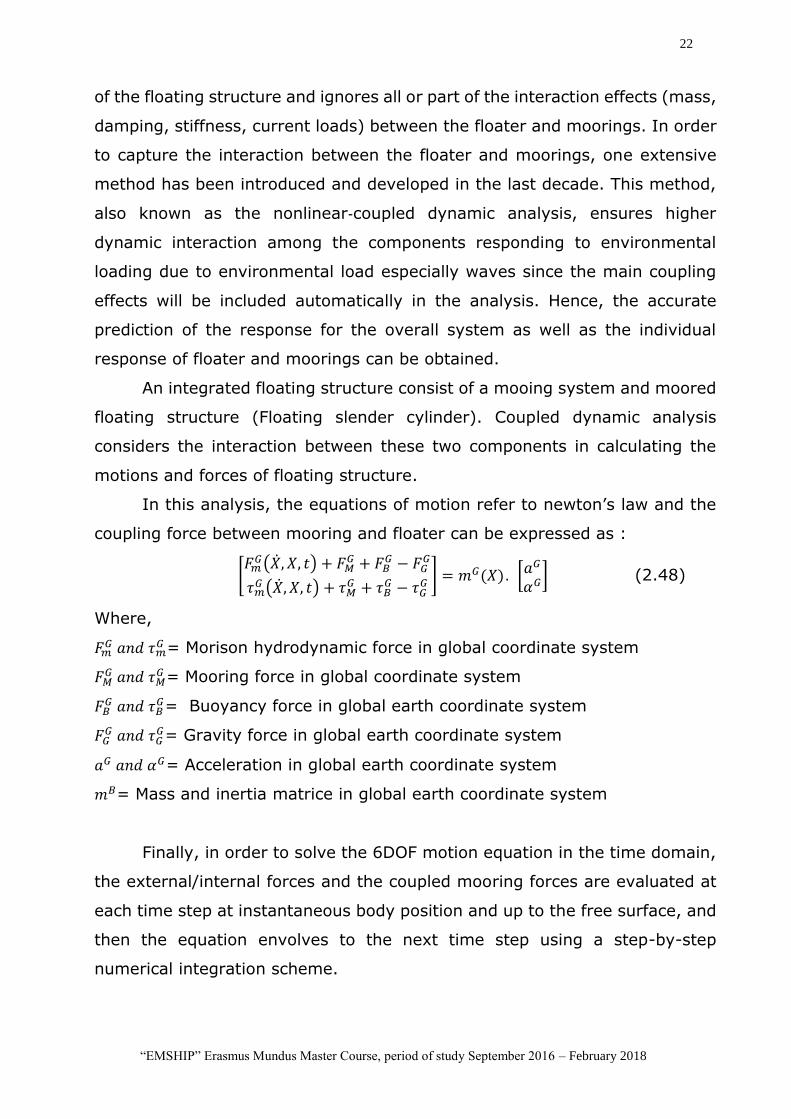
In this analysis, the equations of motion refer to newton’s law and the
coupling force between mooring and floater can be expressed as :
[𝐹𝑚𝐺(�̇�, 𝑋, 𝑡) + 𝐹𝑀
𝐺 + 𝐹𝐵𝐺 − 𝐹𝐺
𝐺
𝜏𝑚𝐺 (�̇�, 𝑋, 𝑡) + 𝜏𝑀
𝐺 + 𝜏𝐵𝐺 − 𝜏𝐺
𝐺] = 𝑚𝐺(𝑋). [𝑎
𝐺
𝛼𝐺] (2.48)
Where,
𝐹𝑚𝐺 𝑎𝑛𝑑 𝜏𝑚
𝐺= Morison hydrodynamic force in global coordinate system
𝐹𝑀𝐺 𝑎𝑛𝑑 𝜏𝑀
𝐺= Mooring force in global coordinate system
𝐹𝐵𝐺 𝑎𝑛𝑑 𝜏𝐵
𝐺= Buoyancy force in global earth coordinate system
𝐹𝐺𝐺 𝑎𝑛𝑑 𝜏𝐺
𝐺= Gravity force in global earth coordinate system
𝑎𝐺 𝑎𝑛𝑑 𝛼𝐺= Acceleration in global earth coordinate system
𝑚𝐵= Mass and inertia matrice in global earth coordinate system
Finally, in order to solve the 6DOF motion equation in the time domain,
the external/internal forces and the coupled mooring forces are evaluated at
each time step at instantaneous body position and up to the free surface, and
then the equation envolves to the next time step using a step-by-step
numerical integration scheme.

23
“EMSHIP” Erasmus Mundus Master Course, period of study September 2016 – February 2018
2.5. Motion and Response Analysis in Time Domain
Finally, the 3 forces and 3 torques due to 6 degree of freedom from
internal, external and coupled mooring forces are resulted from OCN Sim Flex
program due to the morison hydrodynamic equations implementation. In
order to evaluate the morison hydrodynamic equations implementation in the
program, it is necessary to obtain the final result of body motion response and
mooring line tension, then make such a comparative study of those results.
The solution of dynamic equation can be found by frequency domain or
by time domain analysis. Frequency domain analysis will be applicable for the
environmental load that gives satisfactorily results by linearization theory,
while time domain analysis will be performed as direct numerical integration
of the equation of motions which involves non linear functions to predict the
maximum response and capture higher order load effect.
Time domain analysis requires a proper simulation length to have a
steady result. Furthermore, the time domain analysis procedure consist of a
numerical solution of rigid body equation of motion for the floater subject to
external/internal actions which may originate in the fluid motion due to waves,
floater motion, and positioning system. However, in this analysis, a normal
time domain simulation is computed by numerical integration of the equations
of motions.
The loadcases analysis will be evaluated using dynamic analysis in some
stages regarding the mooring configurations. The dynamic analysis of the
system will be performed to asses the global dynamic response.
An acceptable model designed will be combined with 2 condition of
mooring configurations. The effect of changing the mooring configuration for
each condition induced by 4 regular wave loadceses are compared. This stage
analysis will using time domain analysis using OCN Simflex program. The
analysis comprises :
Displacement versus time as motion response
Maximum Line tension
24
“EMSHIP” Erasmus Mundus Master Course, period of study September 2016 – February 2018
As mention in previously, the resulting forces and torques in equation
(4.18) and (4.19) are in global system coordinate. In order to solve the
acceleration which will be an input value in new displacement time step
calculation, it is necessary to transform the resulting forces and torques, from
global, 𝐹𝐺 𝑎𝑛𝑑 𝜏𝐺 , into local body coordinate system, 𝐹𝐵 𝑎𝑛𝑑 𝜏𝐵. The
transformation calculation are present as follows:
𝐹𝐵(𝑡) = 𝑇. 𝐹𝐺 𝑎𝑛𝑑 𝜏𝐵(𝑡) = 𝑇. 𝜏𝐺 (5.1)
Where T is transformaton matrix, equation 4.3. For a floating structures,
it is considered that total mass as well as its distribution over the body is
considered to be constant with time, which the range of time is large relative
to period of motions, this means that small effect can be ignored. The inertia
tensor, 𝐼𝐵 also are transformed to local body coordinate system, the inverse
of inertia tensor is present as follows :
(𝐼𝐵)−1 = 𝑇. 𝐼𝐺 . 𝑇𝑇 (5.2)
Then, the total inverse mass and inertia matrice will be taking into
account both result of above transformation equation as present as follows :
(𝑚𝐵⃗⃗⃗⃗ ⃗⃗ )−1
=
(
𝑀−1 0 00 𝑀−1 00 0 𝑀−1
0 0 0 0 0 00 0 0
0 0 00 0 00 0 0
𝐼𝑥𝑥−1 𝐼𝑥𝑦
−1 𝐼𝑥𝑧−1
𝐼𝑦𝑥−1 𝐼𝑦𝑦
−1 𝐼𝑦𝑧−1
𝐼𝑧𝑥−1 𝐼𝑧𝑦
−1 𝐼𝑧𝑧−1)
(5.3)
Here, we consider moment inertia of cylinder as follows :
𝐼𝑧𝑧𝐵 =
𝑀𝐵 . 𝑟2
2
𝐼𝑥𝑥𝐵 = 𝐼𝑦𝑦
𝐵 =𝑀𝐵.𝑟
2(3𝑟2 + ℎ2) (5.4)
Where, 𝑀𝐵 as mass in local body coordinate system, h as height and r as
radius of solid cylinder, and it is noted that in many application 𝐼𝑥𝑧𝐵 = 𝐼𝑧𝑥
𝐵 is not
known or small, hence their term are neglected.
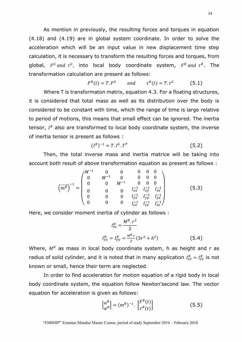
In order to find acceleration for motion equation of a rigid body in local
body coordinate system, the equation follow Newton’second law. The vector
equation for acceleration is given as follows:
[𝑎𝐵
𝛼𝐵] = (𝑚𝐵)−1 . [
𝐹𝐵(𝑡)
𝜏𝐵(𝑡)] (5.5)
25
“EMSHIP” Erasmus Mundus Master Course, period of study September 2016 – February 2018
Where,
𝐹𝐵= resulting external force acting in the center of gravity
𝜏𝐵 = resulting external torque acting about the center of gravity
𝑚𝐵 = mass and moment inertia of rigid body at centre gravity
𝛼𝐵 = angular acceleration of the center of gravity
𝑎𝐵 = acceleration of the center of gravity
T= rotational transformation matrice
t = time
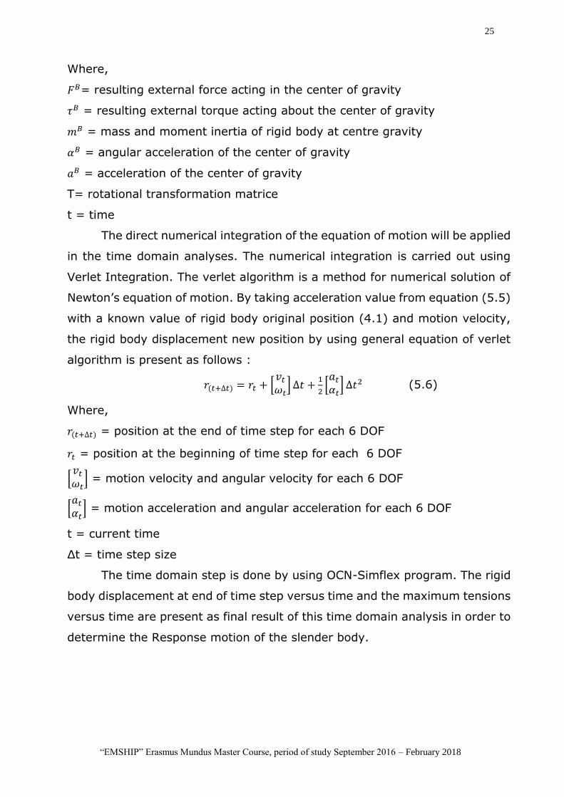
The direct numerical integration of the equation of motion will be applied
in the time domain analyses. The numerical integration is carried out using
Verlet Integration. The verlet algorithm is a method for numerical solution of
Newton’s equation of motion. By taking acceleration value from equation (5.5)
with a known value of rigid body original position (4.1) and motion velocity,
the rigid body displacement new position by using general equation of verlet
algorithm is present as follows :
𝑟(𝑡+∆𝑡) = 𝑟𝑡 + [𝑣𝑡𝜔𝑡] ∆𝑡 +
1
2[𝑎𝑡𝛼𝑡] ∆𝑡2 (5.6)
Where,
𝑟(𝑡+∆𝑡) = position at the end of time step for each 6 DOF
𝑟𝑡 = position at the beginning of time step for each 6 DOF
[𝑣𝑡𝜔𝑡] = motion velocity and angular velocity for each 6 DOF
[𝑎𝑡𝛼𝑡] = motion acceleration and angular acceleration for each 6 DOF
t = current time
Δt = time step size
The time domain step is done by using OCN-Simflex program. The rigid
body displacement at end of time step versus time and the maximum tensions
versus time are present as final result of this time domain analysis in order to
determine the Response motion of the slender body.
26
“EMSHIP” Erasmus Mundus Master Course, period of study September 2016 – February 2018
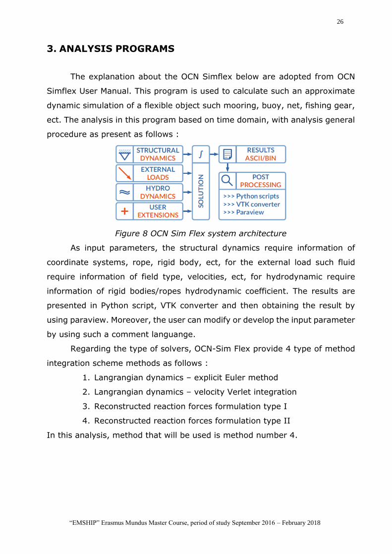
3. ANALYSIS PROGRAMS
The explanation about the OCN Simflex below are adopted from OCN
Simflex User Manual. This program is used to calculate such an approximate
dynamic simulation of a flexible object such mooring, buoy, net, fishing gear,
ect. The analysis in this program based on time domain, with analysis general
procedure as present as follows :
Figure 8 OCN Sim Flex system architecture
As input parameters, the structural dynamics require information of
coordinate systems, rope, rigid body, ect, for the external load such fluid
require information of field type, velocities, ect, for hydrodynamic require
information of rigid bodies/ropes hydrodynamic coefficient. The results are
presented in Python script, VTK converter and then obtaining the result by
using paraview. Moreover, the user can modify or develop the input parameter
by using such a comment languange.
Regarding the type of solvers, OCN-Sim Flex provide 4 type of method
integration scheme methods as follows :
1. Langrangian dynamics – explicit Euler method
2. Langrangian dynamics – velocity Verlet integration
3. Reconstructed reaction forces formulation type I
4. Reconstructed reaction forces formulation type II
In this analysis, method that will be used is method number 4.
27
“EMSHIP” Erasmus Mundus Master Course, period of study September 2016 – February 2018
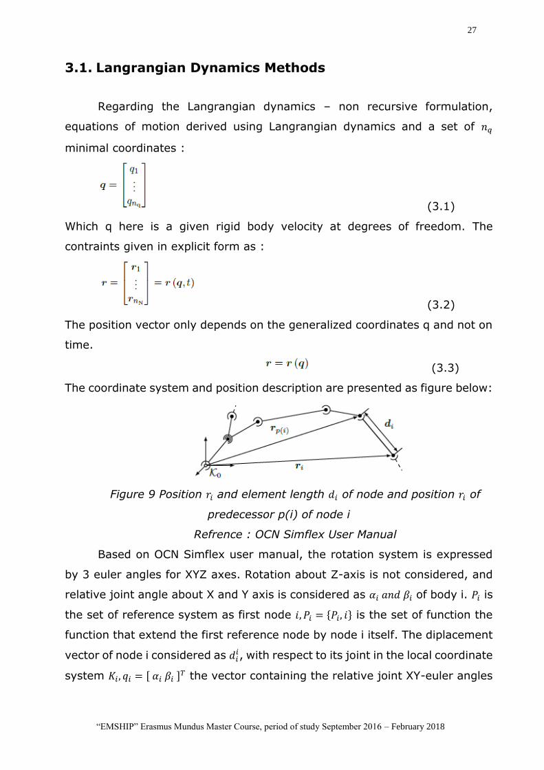
3.1. Langrangian Dynamics Methods
Regarding the Langrangian dynamics – non recursive formulation,
equations of motion derived using Langrangian dynamics and a set of 𝑛𝑞
minimal coordinates :
(3.1)
Which q here is a given rigid body velocity at degrees of freedom. The
contraints given in explicit form as :
(3.2)
The position vector only depends on the generalized coordinates q and not on
time.
(3.3)
The coordinate system and position description are presented as figure below:
Figure 9 Position 𝑟𝑖 and element length 𝑑𝑖 of node and position 𝑟𝑖 of
predecessor p(i) of node i
Refrence : OCN Simflex User Manual
Based on OCN Simflex user manual, the rotation system is expressed
by 3 euler angles for XYZ axes. Rotation about Z-axis is not considered, and
relative joint angle about X and Y axis is considered as 𝛼𝑖 𝑎𝑛𝑑 𝛽𝑖 of body i. 𝑃𝑖 is
the set of reference system as first node 𝑖, 𝑃𝑖 = {𝑃𝑖, 𝑖} is the set of function the
function that extend the first reference node by node i itself. The diplacement
vector of node i considered as 𝑑𝑖𝑖, with respect to its joint in the local coordinate
system 𝐾𝑖, 𝑞𝑖 = [ 𝛼𝑖 𝛽𝑖 ]𝑇 the vector containing the relative joint XY-euler angles
28
“EMSHIP” Erasmus Mundus Master Course, period of study September 2016 – February 2018
𝛼𝑖 as well as 𝛽𝑖 and 𝑇0𝑘 the transformation matrix from 𝐾𝑖 to the reference
system 𝐾𝑖.
For the transformation rotation , The position 𝑟𝑖0 of node i is evaluated
in the global earth coordinate system, 𝐾0 is the sum of all displacement vectors
of it’s previous references nodes 𝑃𝑖.
In order to calculate velocity projection, jacobian matrice 𝐽𝑖𝑗 , 𝑗 ∈ 𝑃�̅� as well
as the associated joint velocities 𝑞𝑖𝑗 , 𝑗 ∈ 𝑃�̅� can be combined with joint velocities
q onto the Cartesian velocities of node i as follows :
(3.4)
with masspoint’s Jacobian matrix with respect to joint 𝐽𝑖𝑗 , 𝑗 ∈ 𝑃�̅� :
(3.5)
With S as derivatves expression, While for 𝐽𝑖𝑗, 𝑗 ∉ 𝑃�̅� , the velocity projection
vector is :
(3.6)
Here all submatrices 𝐽𝑖𝑗 become 0(3,2) if , 𝑗 ∉ 𝑃�̅� and the masspoint’s Jacobian
matrix needs to be extended to :
(3.7)
By physical interpretation, an expression equation can be arranged as :
(3.8)
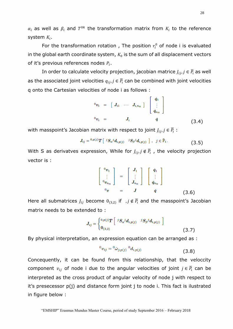
Concequently, it can be found from this relationship, that the veloccity
component 𝑣𝑖𝑗 of node i due to the angular velocities of joint 𝑗 ∈ 𝑃�̅� can be
interpreted as the cross product of angular velocity of node j with respect to
it’s presecessor p(j) and distance form joint j to node i. This fact is ilustrated
in figure below :
29
“EMSHIP” Erasmus Mundus Master Course, period of study September 2016 – February 2018
Figure 10 Velocity component 𝑣𝑖𝑗
Refrence : OCN Simflex User Manual
Accelerations, can be found by differentiating equation 3.7 with respect
to time and leads the system’s vector of accelerations :
(3.9)
The derivation of Jacobian with respect to time leads to quadratic terms
in the joint velocities �̇� in the last term in the above equation. By ignoring high
frequent vibrations induced e.g by vortexes, the time derivatives of the joint
angles are typically very small, i.e. �̇� ≪ 1. Consequently the resulting quadratic
velocity terms can be neglected resuting in :
(3.10)
For equation of motion, applying the principle of virtual power, the
equationsof motion of all nodes can be derived as :
(3.11)
The upper left index indicating the coordinate system is omitted. The
subtitution of cartesian acceleration leads to :
(3.12)
Because the reaction fforces are perpendicular to the constraint manifold,
which is defined by the columns of the Jacobian matrix, the system’s
generalised mass matrix :
(3.13)
The vector of generalised external forces become:
30
“EMSHIP” Erasmus Mundus Master Course, period of study September 2016 – February 2018
(3.14)
Equation above can be assumed as projections of the respective inertia and
external forces to the constraint manifold.
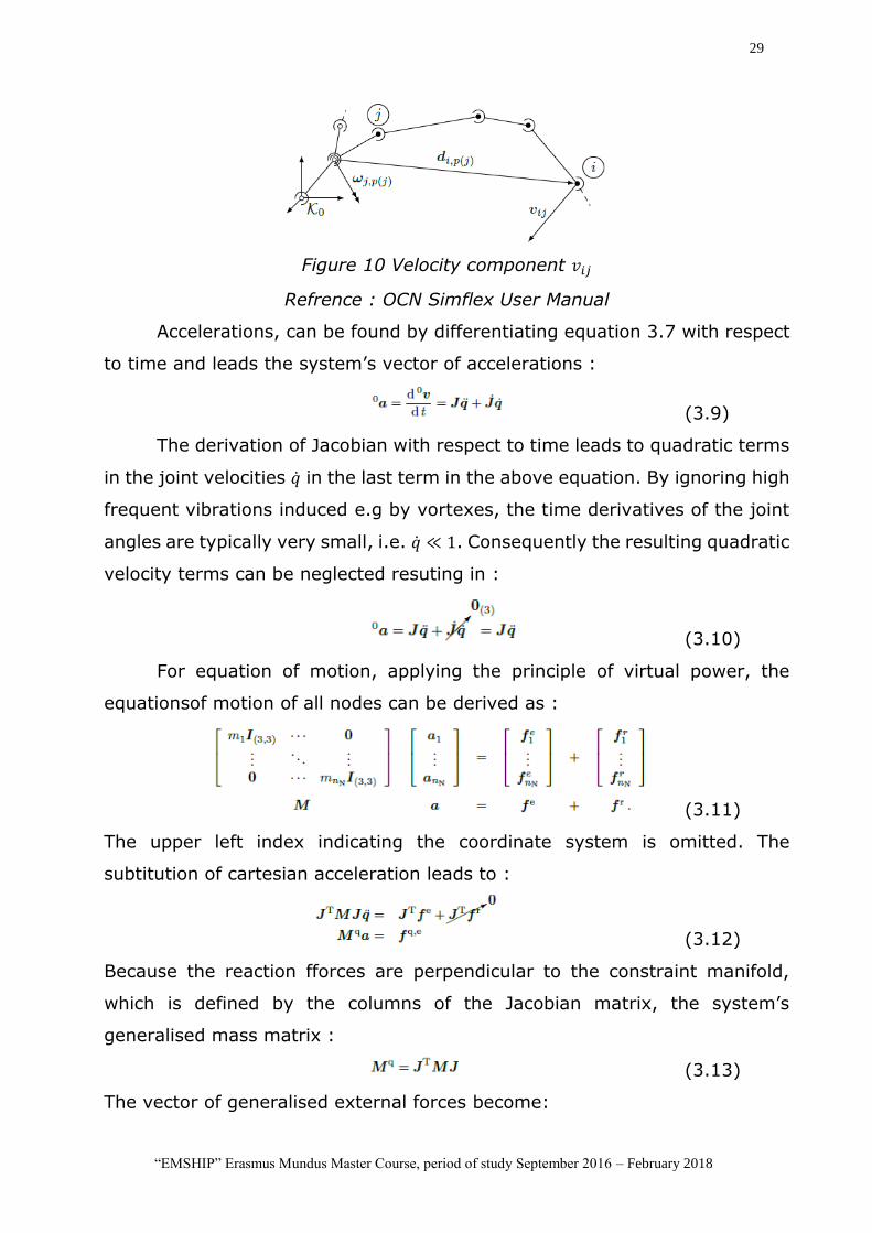
3.2. Reconstructed Reaction Forces Formulation Methods
This method using Langrangian classical method – Langrangian
dynamic, which based on explicit constraint equations and minimal
coordinates or implicit constraint equations and redundant coordinates.
Depending on choice of formulation exact solution of constraints (explicit
equations) or violatoin of cinstraints due to numerical integration of
constraints (implicit constraints).
Figure 11 Example pendulum. a) Exact solution of explicit contraints
equations b) Violation of constraints due to numerical integration of implicit constraint equations. Violation corrected by projection.
Rerence : OCN Simflex User Manual
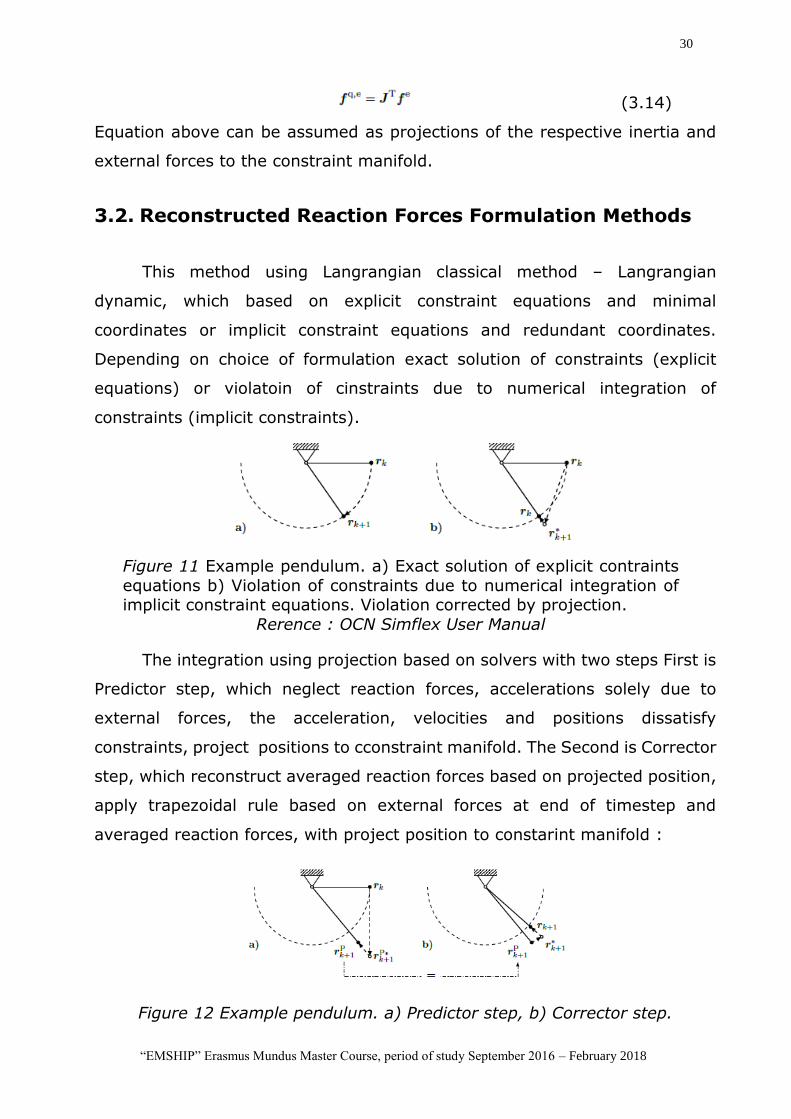
The integration using projection based on solvers with two steps First is
Predictor step, which neglect reaction forces, accelerations solely due to
external forces, the acceleration, velocities and positions dissatisfy
constraints, project positions to cconstraint manifold. The Second is Corrector
step, which reconstruct averaged reaction forces based on projected position,
apply trapezoidal rule based on external forces at end of timestep and
averaged reaction forces, with project position to constarint manifold :
Figure 12 Example pendulum. a) Predictor step, b) Corrector step.
31
“EMSHIP” Erasmus Mundus Master Course, period of study September 2016 – February 2018
Refrence : OCN Simflex User Manual
The equation of motion based on Langrangian dynamic and dependant
cooordinate (primary constraints given in implicit form) as :
(3.15)
Where the position vector only depends on the generalized coordinates q, the
constrant vector is expressed as :
(3.16)
Rotation projection which is using XYZ euler joint angles is the same as
Langrangian dynamic method at previous chapter.
The projected positions r should fullfil the constraint condition above
because for projection position, The relaxation algorithm, the position 𝑟∗
violating the constraint equations back towards the constraint manifold, the
operator r is expressed as :
(3.17)
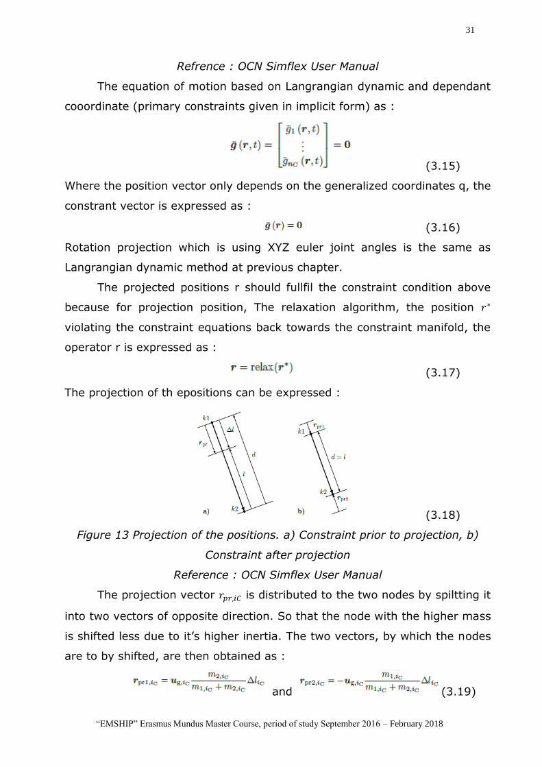
The projection of th epositions can be expressed :
(3.18)
Figure 13 Projection of the positions. a) Constraint prior to projection, b)
Constraint after projection
Reference : OCN Simflex User Manual
The projection vector 𝑟𝑝𝑟,𝑖𝐶 is distributed to the two nodes by spiltting it
into two vectors of opposite direction. So that the node with the higher mass
is shifted less due to it’s higher inertia. The two vectors, by which the nodes
are to by shifted, are then obtained as :
and (3.19)
32
“EMSHIP” Erasmus Mundus Master Course, period of study September 2016 – February 2018
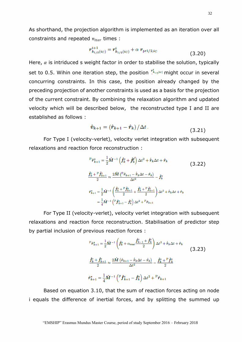
As shorthand, the projection algorithm is implemented as an iteration over all
constraints and repeated 𝑛𝐼𝑡𝑒𝑟 times :
(3.20)
Here, 𝛼 is intriduced s weight factor in order to stabilise the solution, typically
set to 0.5. Wihin one iteration step, the position might occur in several
concurring constraints. In this case, the position already changed by the
preceding projection of another constraints is used as a basis for the projection
of the current constraint. By combining the relaxation algorithm and updated
velocity which will be described below, the reconstructed type I and II are
established as follows :
(3.21)
For Type I (velocity-verlet), velocity verlet integration with subsequent
relaxations and reaction force reconstruction :
(3.22)
For Type II (velocity-verlet), velocity verlet integration with subsequent
relaxations and reaction force reconstruction. Stabilisation of predictor step
by partial inclusion of previous reaction forces :
(3.23)
Based on equation 3.10, that the sum of reaction forces acting on node
i equals the difference of inertial forces, and by splitting the summed up
33
“EMSHIP” Erasmus Mundus Master Course, period of study September 2016 – February 2018
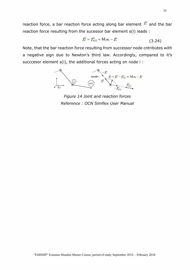
reaction force, a bar reaction force acting along bar element and the bar
reaction force resulting from the sucessor bar element s(i) leads :
(3.24)
Note, that the bar reaction force resulting from successor node cntributes with
a negative sign due to Newton’s third law. Accordingly, compared to it’s
succcesor element s(i), the additional forces acting on node i :
Figure 14 Joint and reaction forces
Reference : OCN Simflex User Manual
34
“EMSHIP” Erasmus Mundus Master Course, period of study September 2016 – February 2018
4. HYDRODYNAMIC FORCES ON FLOATING CYLINDRICAL
STRUCTURE AND MOORING LINE
4.1. Implementation of Alghotythm in Matlab
The dynamic movement of fluids can be expressed in mathematical
formulas by using MATLAB software as one of Mathematical Modelling
Languange application. The primary purpose is to develop an algorithm for
the numeric integration of hydrodynamic loads on slender cylindrical objects
by using morison equation. The hydrodynamic load of the objects here consist
of the floater and the mooring line. Subsequently, the plausibility of the
developed algorithm has to be checked.
There are several steps of equation implementations in order to arrive
to the hydrodynamic force result. The hydrodynamic force alghorythms are
presented in for 2 object, the cylindrical floating structure and the mooring
line. The hydrodynamic force alghorythm of cylindrical structure is defined as
follows :
1. Cylinder position and velocity vector at coordinate system using
transformation matrix calculation
2. Wave elevation calculation
3. Airy wave velocitiy at every marker point on the cylinder at x and z axes
4. Relative Velocity between cylinder structure and wave
5. Transformation of relative velocity and filtering result with respect to
wave elevation
6. Drag Coefficient
7. Hydrodynamic Morison forces equation, with respect to drag force due
to viscosity only
While, the hydrodynamic force alghorythm of mooring line is defined as
follows:
1. Mooring line position, velocity and acceleration vector at coordinate
system
2. Wave elevation calculation
35
“EMSHIP” Erasmus Mundus Master Course, period of study September 2016 – February 2018
3. Airy wave velocitiy and acceleration at every marker point on the
mooring line at x and z axes
4. Relative Velocity and acceleration between mooring line and wave
5. Transformation of relative velocity and acceleration and filtering result
with respect to wave elevation
6. Added mass and Drag Coefficient
7. Hydrodynamic Morison forces equation, with respect to froude krylov,
hydrodybanic mass and drag force
The detail Matlab codes of Morison hydrodynamic algorithm and the plausible
sample result are present in appendix B and C.
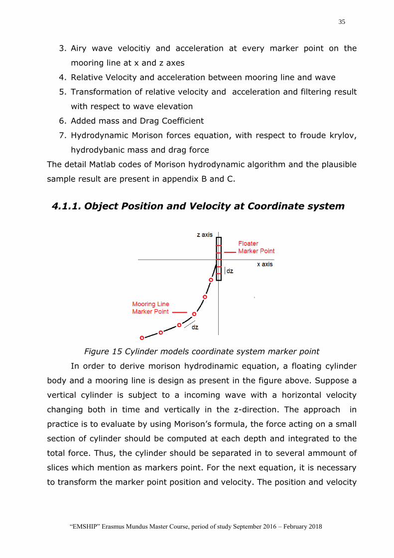
4.1.1. Object Position and Velocity at Coordinate system
Figure 15 Cylinder models coordinate system marker point
In order to derive morison hydrodinamic equation, a floating cylinder
body and a mooring line is design as present in the figure above. Suppose a
vertical cylinder is subject to a incoming wave with a horizontal velocity
changing both in time and vertically in the z-direction. The approach in
practice is to evaluate by using Morison’s formula, the force acting on a small
section of cylinder should be computed at each depth and integrated to the
total force. Thus, the cylinder should be separated in to several ammount of
slices which mention as markers point. For the next equation, it is necessary
to transform the marker point position and velocity. The position and velocity
36
“EMSHIP” Erasmus Mundus Master Course, period of study September 2016 – February 2018
transformation from local body coordinate to global earth coordinate in matlab
are defined as follows :
𝑟𝐺 = 𝑟𝑟𝑒𝑓𝐺 + (𝑇. 𝑟𝐵) (4.1)
𝑣𝐺 = 𝑣𝑟𝑒𝑓𝐺 + (𝜔. 𝑇. 𝑟𝐵) (4.2)
where,
𝑟𝐺 = positions of markers at global earth coordinate system
𝑟𝐵 = positions of markers at local body coordinate system
𝑣𝐺 = velocity of markers at local body coordinate system
𝑟𝑟𝑒𝑓𝐺 = Position of body Reference at global earth coordinate system
𝑣𝑟𝑒𝑓𝐺 = Velocity of body Reference at global earth coordinate system
T = Transformation Matrix between the local body fixed coordinate system
and the global earth fixed coordinate system expressed as :
(4.3)
T is an orthogonal matrix with the property that 𝑇𝑇 = 𝑇−1, with (𝛼1, 𝛼2, 𝛼3) as
euler angle.
For the mooring line hydrodynamic position, velocity and acceleration,
are assumed as a moving marker point at each segment except for the anchor
point which is assumed as fixed point. Therefore, the velocity and acceleration
at this point is assumed equal to zero.
4.1.2. Wave Elevation
The implementation in matlab for wave elevation of a long-crested
regular wave, propagating along the positive x axis, in time variant is written
as follows :
(4.4)
Where,
𝜉𝑎 = wave amplitude
37
“EMSHIP” Erasmus Mundus Master Course, period of study September 2016 – February 2018
k = wave number
𝜔 =2𝜋
𝑇
t = time variant
The form of water surface equation above is simulated that the wave
moves in the positive x-direction. The wave elevation is defined for each
marker point at x and z axes due to time variant. In the implementation for
the cylinrical floater, all the result value such relative velocity, hydrodynamic
morison equation at each marker point along x and z axes will be filtered and
only considered the result for the marker point below the wave elevation (the
submerged part). While the hydrodynamic load result for mooring line is taken
for all marker point since all part of mooring line is designed always below the
wave elevation.
4.1.3. Airy Wave Velocity and Acceleration
The velocity and acceleration as one of components for hydrodynamic
equation are calculated in linear wave theory, further, the theory also known
as Airy wave theory (first order potential theory). Since the vertical cylinder
will be modelled as a floating body, the velocity and acceleration will be
considered coming from 2 axis vertical and horizontal. The equation of velocity
of airy wave theory acting from x and z direction are shown as follows :
𝑢𝑤𝑎𝑣𝑒𝐺 = 𝜉𝑎𝜔
cosh 𝑘(𝑧+𝑑)
sinh 𝑘𝑑cos (𝑘𝑥 − 𝜔𝑡) (4.6)
𝑤𝑤𝑎𝑣𝑒𝐺 = 𝜉𝑎𝜔
sinh 𝑘(𝑧 + 𝑑)
sinh 𝑘𝑑sin (𝑘𝑥 − 𝜔𝑡)
while for the acceleration of airy wave, are shown as follows :
�̇�𝑤𝑎𝑣𝑒𝐺 = 𝜉𝑎𝜔
2 cosh 𝑘(𝑧+𝑑)
sinh 𝑘𝑑sin (𝑘𝑥 − 𝜔𝑡) (4.7)
�̇�𝑤𝑎𝑣𝑒𝐺 = −𝜉𝑎𝜔
2sinh 𝑘(𝑧 + 𝑑)
sinh 𝑘𝑑cos (𝑘𝑥 − 𝜔𝑡)
Where :
𝑢𝑤𝑎𝑣𝑒𝐺 𝑎𝑛𝑑 𝑤𝑤𝑎𝑣𝑒
𝐺 = wave velocity in horizontal and vertical direction in Global
coord. system
38
“EMSHIP” Erasmus Mundus Master Course, period of study September 2016 – February 2018
�̇�𝑤𝑎𝑣𝑒𝐺 𝑎𝑛𝑑 �̇�𝑤𝑎𝑣𝑒
𝐺 = wave acceleration in horizontal and vertical direction in
Global coord. syst.
𝜉𝑎 = wave amplitude
𝜔 =2𝜋
𝑇
T = period
k = wave number
d = sea depth
t = variant value of time set
x = variant value of domain position of cylinder in x axis (divided to n marker
point in x axes)
z = vertical length of each stripes cylindrical at submerged body (divided to n
marker point in z axes)
The velocity and acceleration of the wave are calculated by taking into
account the phase angle of the wave as well as the respective diving depth of
the cylindrical floater and mooring line section.
Overall the input value for the velocity of airy wave theory are range
value of domain space (x), time (t) and (z), and the other independent input
value are wave amplitude (𝜉𝑎), depth (d), period (T) and wave length (𝜆) since
omega (𝜔) and wave number (k) can be obtained as follows :
𝜔 =2𝜋
𝑇 (4.8)
𝑘 =2𝜋
𝜆 (4.9)
Furthermore, the wave velocity is used for relative velocity calculation
between the velocity of wave and velocity of cylinder structure for morison
equation of the floater, which is considered as moving floating structure.
While, for the wave acceleration is used directly for morison equation of
mooring line which is considered as fixed structure.
4.1.4. Relative Velocity
The implementation of wave flow velocity both in horizontal and vertical
axes in morison hydrodynamic force equation for cylindrical floater use
39
“EMSHIP” Erasmus Mundus Master Course, period of study September 2016 – February 2018
relative velocity between the body structure and wave flow as shown as
follows :
(𝑢𝑟𝑒𝑙𝐺 = 𝑢𝑤𝑎𝑣𝑒 − 𝑢𝑏𝑜𝑑𝑦) 𝑎𝑛𝑑 ( 𝑤𝑟𝑒𝑙
𝐺 = 𝑤𝑤𝑎𝑣𝑒 − 𝑤𝑏𝑜𝑑𝑦) (4.10)
(�̇�𝑟𝑒𝑙𝐺 = �̇�𝑤𝑎𝑣𝑒 − �̇�𝑏𝑜𝑑𝑦) 𝑎𝑛𝑑 ( �̇�𝑟𝑒𝑙
𝐺 = �̇�𝑤𝑎𝑣𝑒 − �̇�𝑏𝑜𝑑𝑦)
Where,
𝑢𝑟𝑒𝑙𝐺 = relative velocity in horizontal direction
𝑢𝑤𝑎𝑣𝑒= wave flow velocity in horizontal direction
𝑢𝑏𝑜𝑑𝑦= new projection of body structure velocity in horizontal direction
𝑤𝑟𝑒𝑙𝐺 = relative velocity in vertical direction
𝑤𝑤𝑎𝑣𝑒= wave flow velocity in vertical direction
𝑤𝑏𝑜𝑑𝑦= new projection of body structure velocity in vertical direction
4.1.5. Transformation of relative velocity, acceleration and
filtering result with respect to wave elevation
The resulting relative velocity and wave flow acceleration are in global
earth coordinate system. Since the velocity and acceleration in the morison
hydrodinamic force equation should be implemented in local body coordinate
system, therefore, those result should be transform from global earth
coordinate to local body coordinate which is implemented in matlab as follows:
𝑢𝑟𝑒𝑙𝐵 = (𝜔𝑣. 𝑇
𝑇 . 𝑟𝐺) + 𝑢𝑟𝑒𝑙𝐺 𝑎𝑛𝑑 𝑤𝑟𝑒𝑙
𝐵 = (𝜔𝑣. 𝑇𝑇 . 𝑟𝐺) + 𝑤𝑟𝑒𝑙
𝐺 (4.11)
Where,
𝑢𝑟𝑒𝑙𝐵 = Horizontal relative velocity in local coordinate system
𝑤𝑟𝑒𝑙𝐵 = Vertical relative velocity in local coordinate system
𝑢𝑟𝑒𝑙𝐺 = Horizontal relative velocity in local coordinate system
𝑤𝑟𝑒𝑙𝐺 = Vertical relative velocity in local coordinate system
𝜔𝑣 = Angular velocity of floating body
𝑇𝑇 = Transpose of transformation matrix
𝑟𝐺 = position vector in global coordinat system
With 𝜔𝑣 in this equation as angular velocity. After obtaining the resulting
velocity transformation in local body coordinate system, it is necessary also
to filter the result which acting with respect to submerged cylinder part only,
40
“EMSHIP” Erasmus Mundus Master Course, period of study September 2016 – February 2018
hence, the result will be filtered with respect to submerged part below wave
elevation only. It mean the result of velocity and acceleration which respect
to the cylinder body marker points above wave elevation will be neglected.
For further detail about the code, can be seen in the appendix D.
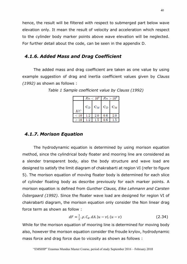
4.1.6. Added Mass and Drag Coefficient
The added mass and drag coefficient are taken as one value by using
example suggestion of drag and inertia coefficient values given by Clauss
(1992) as shown as follows :
Table 1 Sample coefficient value by Clauss (1992)
4.1.7. Morison Equation
The hydrodynamic equation is determined by using morison equation
method, since the cylindrical body floater and mooring line are considered as
a slender transparent body, also the body structure and wave load are
designed to satisfy the limit diagram of chakrabarti at region VI (refer to figure
5). The morison equation of moving floater body is determined for each slice
of cylinder floating body as describe previously for each marker points. A
morison equation is defined from Gunther Clauss, Eike Lehmann and Carsten
�̈�stergaard (1992). Since the floater wave load are designed for region VI of
chakrabarti diagram, the morison equation only consider the Non linear drag
force term as shown as follow :
𝑑𝐹 =1
2. 𝜌. 𝐶𝑑. 𝑑𝐴. |𝑢 − 𝑣|. (𝑢 − 𝑣) (2.34)
While for the morison equation of mooring line is determined for moving body
also, however the morison equation consider the froude krylov, hydrodynamic
mass force and drag force due to vicosity as shown as follows :

41
“EMSHIP” Erasmus Mundus Master Course, period of study September 2016 – February 2018
𝑑𝐹𝑥 = 𝜌. 𝑑∀.𝜕𝑢
𝜕𝑡− 𝜌. 𝐶𝑎. 𝑑∀. (
𝜕𝑢
𝜕𝑡− 𝑢�̇�) +
1
2. 𝜌. 𝐶𝑑 . 𝑑𝐴. |𝑢 − 𝑣|. (𝑢 − 𝑣) (2.33)
Cm = (1+Ca) = inertia coefficient with 𝐶𝑎 as added mass coefficient
Cd = Drag coefficient
dz = separated vertical distance in z axis
𝑑∀ = Volume of submerged cylinder
dA = The cross sectional which perpendicular to flow direction
r = half of diameter
D = Diameter of cylinder
u = Wave flow velocity
𝑣 = Body structure velocity
𝜕𝑢
𝜕𝑡= Wave flow acceleration
�̇�𝑐= Body structure acceleration
The added mass and drag coefficient will consider one coefficient for any
stripes/marker point using approach sample from Claus (1992).
4.2. Plaussible Results
A plaussible results of Morison Force equation are obtained to be
checked for both objects, cylinder structure boody and mooring line. The input
value of objects design geometry and wave loadcase are designed as similar
as possible for both object for the comparison study result, the input are
presented as follows :
Loadcases Value
Depth-d (m) 16.0
Wave Height-H (m) 5.4
Amplitude-A (m) 2.7
Period-T (s) 5.0
Frequency-f (Hz) 0.2
Horizontal Wave
Velocity-v (m/s) 1.0
42
“EMSHIP” Erasmus Mundus Master Course, period of study September 2016 – February 2018
Omega-ω 1.3
Wave Numb. (rad/m) 0.3
Wave Length-L (m) 30.0
H/D (>=20) 20.0
𝜋𝐷/𝐿 (<=0.03) 0.02
Structure Velocity-x (m/s) 1.0
Structure Acceleration-x (m/s2) 1.0
nMarkers 11.0
Cylinder Floating Structure
Diameter of Cylinder (m) 2.7
Length of Cylinder (m) 12.0
Mooring Line
Diameter of Line (m) 2.7
Length of Line (m) 12.0
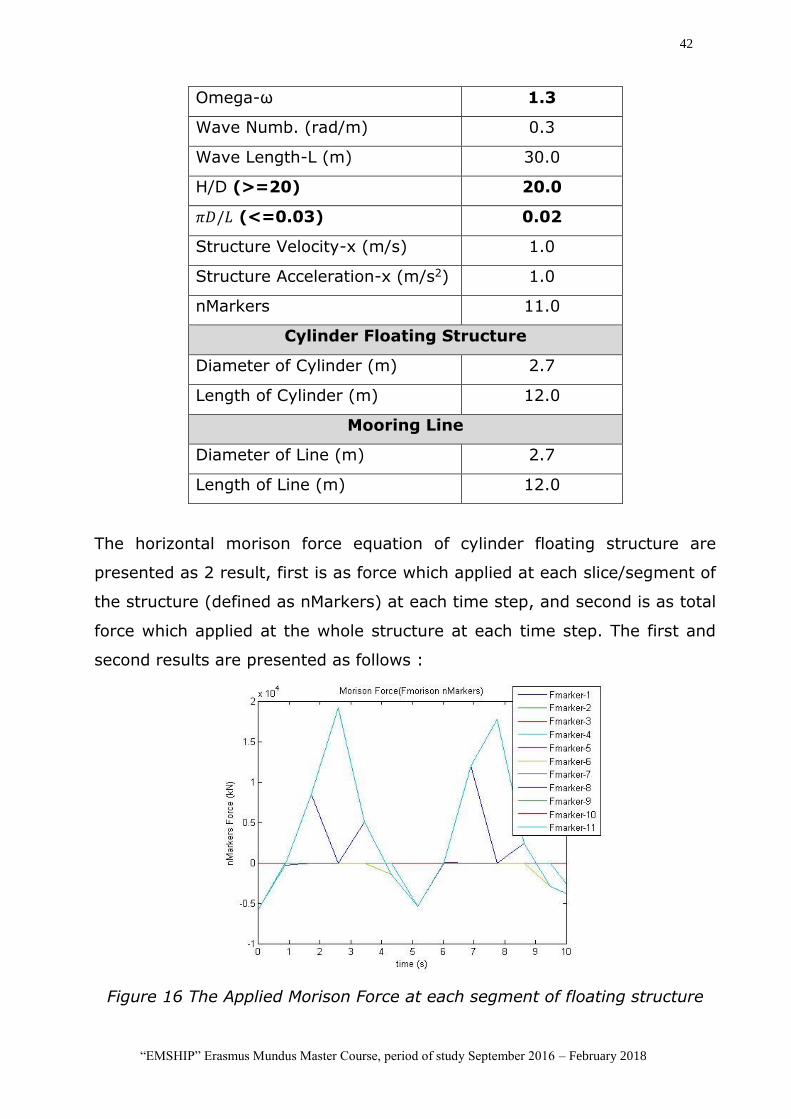
The horizontal morison force equation of cylinder floating structure are
presented as 2 result, first is as force which applied at each slice/segment of
the structure (defined as nMarkers) at each time step, and second is as total
force which applied at the whole structure at each time step. The first and
second results are presented as follows :
Figure 16 The Applied Morison Force at each segment of floating structure
43
“EMSHIP” Erasmus Mundus Master Course, period of study September 2016 – February 2018
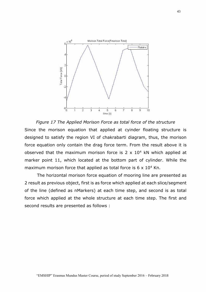
Figure 17 The Applied Morison Force as total force of the structure
Since the morison equation that applied at cyinder floating structure is
designed to satisfy the region VI of chakrabarti diagram, thus, the morison
force equation only contain the drag force term. From the result above it is
observed that the maximum morison force is 2 x 10⁴ kN which applied at
marker point 11, which located at the bottom part of cylinder. While the
maximum morison force that applied as total force is 6 x 10⁴ Kn.
The horizontal morison force equation of mooring line are presented as
2 result as previous object, first is as force which applied at each slice/segment
of the line (defined as nMarkers) at each time step, and second is as total
force which applied at the whole structure at each time step. The first and
second results are presented as follows :
44
“EMSHIP” Erasmus Mundus Master Course, period of study September 2016 – February 2018
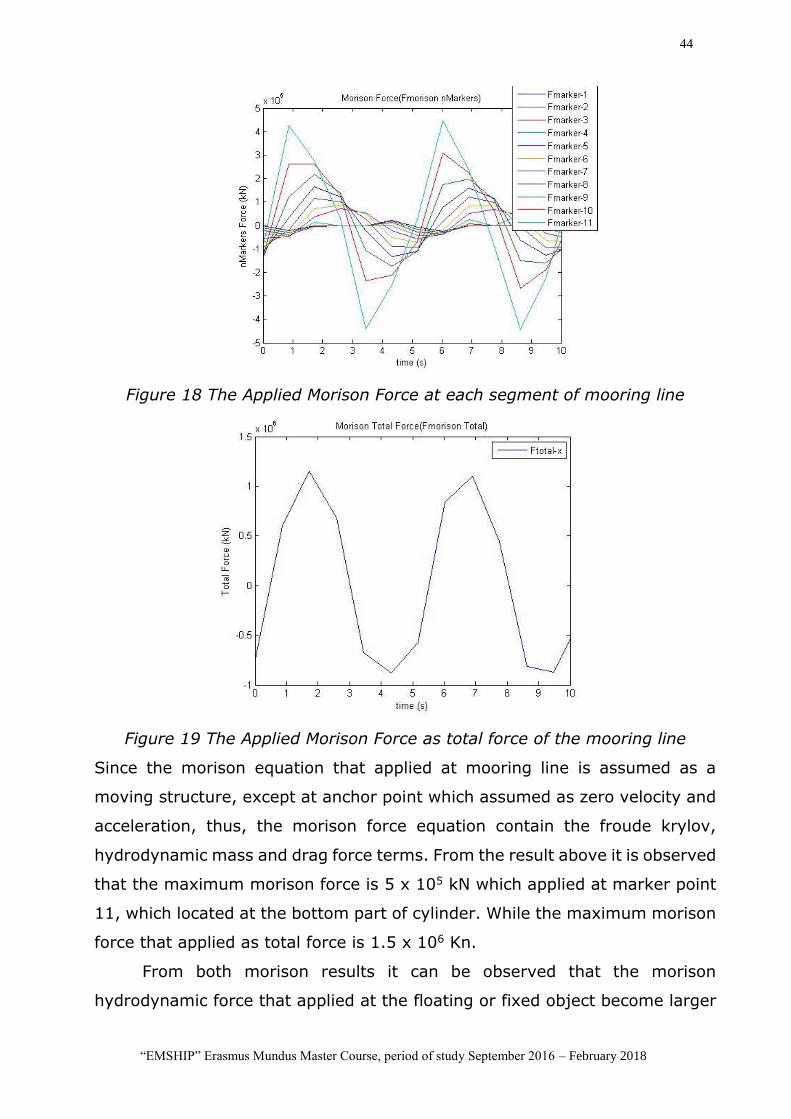
Figure 18 The Applied Morison Force at each segment of mooring line
Figure 19 The Applied Morison Force as total force of the mooring line
Since the morison equation that applied at mooring line is assumed as a
moving structure, except at anchor point which assumed as zero velocity and
acceleration, thus, the morison force equation contain the froude krylov,
hydrodynamic mass and drag force terms. From the result above it is observed
that the maximum morison force is 5 x 10⁵ kN which applied at marker point
11, which located at the bottom part of cylinder. While the maximum morison
force that applied as total force is 1.5 x 10⁶ Kn.
From both morison results it can be observed that the morison
hydrodynamic force that applied at the floating or fixed object become larger
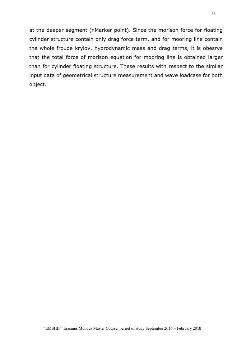
45
“EMSHIP” Erasmus Mundus Master Course, period of study September 2016 – February 2018
at the deeper segment (nMarker point). Since the morison force for floating
cylinder structure contain only drag force term, and for mooring line contain
the whole froude krylov, hydrodynamic mass and drag terms, it is obesrve
that the total force of morison equation for mooring line is obtained larger
than for cylinder floating structure. These results with respect to the similar
input data of geometrical structure measurement and wave loadcase for both
object.
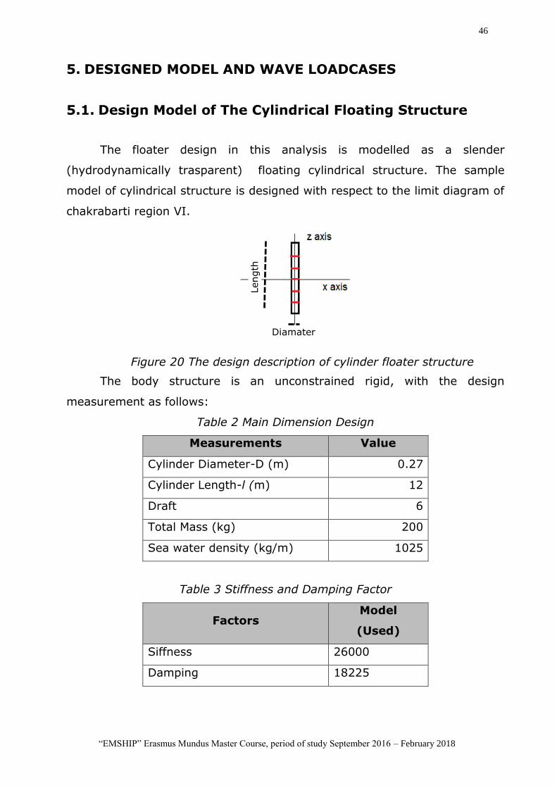
46
“EMSHIP” Erasmus Mundus Master Course, period of study September 2016 – February 2018
5. DESIGNED MODEL AND WAVE LOADCASES
5.1. Design Model of The Cylindrical Floating Structure
The floater design in this analysis is modelled as a slender
(hydrodynamically trasparent) floating cylindrical structure. The sample
model of cylindrical structure is designed with respect to the limit diagram of
chakrabarti region VI.
Figure 20 The design description of cylinder floater structure
The body structure is an unconstrained rigid, with the design
measurement as follows:
Table 2 Main Dimension Design
Measurements Value
Cylinder Diameter-D (m) 0.27
Cylinder Length-l (m) 12
Draft 6
Total Mass (kg) 200
Sea water density (kg/m) 1025
Table 3 Stiffness and Damping Factor
Factors Model
(Used)
Siffness 26000
Damping 18225
Diamater
Length
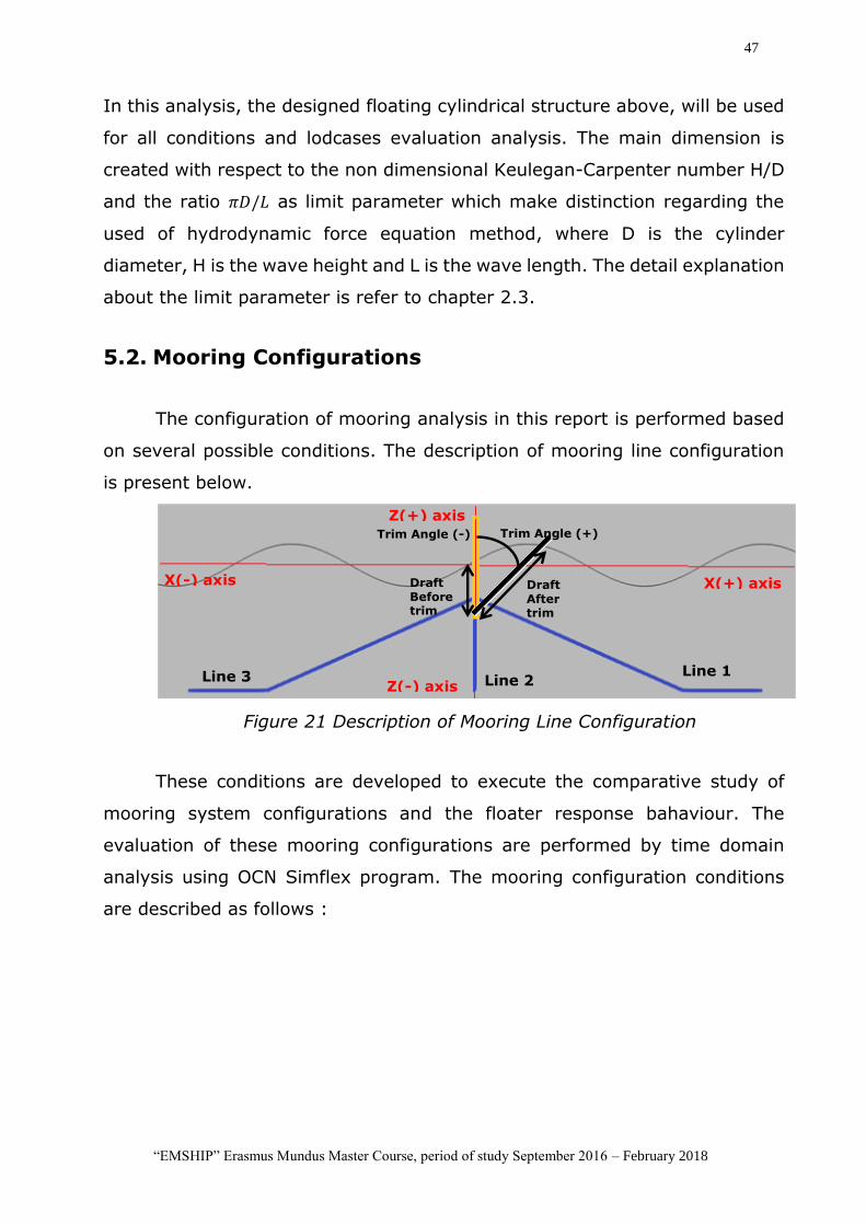
47
“EMSHIP” Erasmus Mundus Master Course, period of study September 2016 – February 2018
In this analysis, the designed floating cylindrical structure above, will be used
for all conditions and lodcases evaluation analysis. The main dimension is
created with respect to the non dimensional Keulegan-Carpenter number H/D
and the ratio 𝜋𝐷/𝐿 as limit parameter which make distinction regarding the
used of hydrodynamic force equation method, where D is the cylinder
diameter, H is the wave height and L is the wave length. The detail explanation
about the limit parameter is refer to chapter 2.3.
5.2. Mooring Configurations
The configuration of mooring analysis in this report is performed based
on several possible conditions. The description of mooring line configuration
is present below.
Figure 21 Description of Mooring Line Configuration
These conditions are developed to execute the comparative study of
mooring system configurations and the floater response bahaviour. The
evaluation of these mooring configurations are performed by time domain
analysis using OCN Simflex program. The mooring configuration conditions
are described as follows :
Line 1 Line 3 Line 2
X(+) axis X(-) axis
Z(+) axis
Z(-) axis
Trim Angle (+) Trim Angle (-)
Draft Before trim
Draft After trim
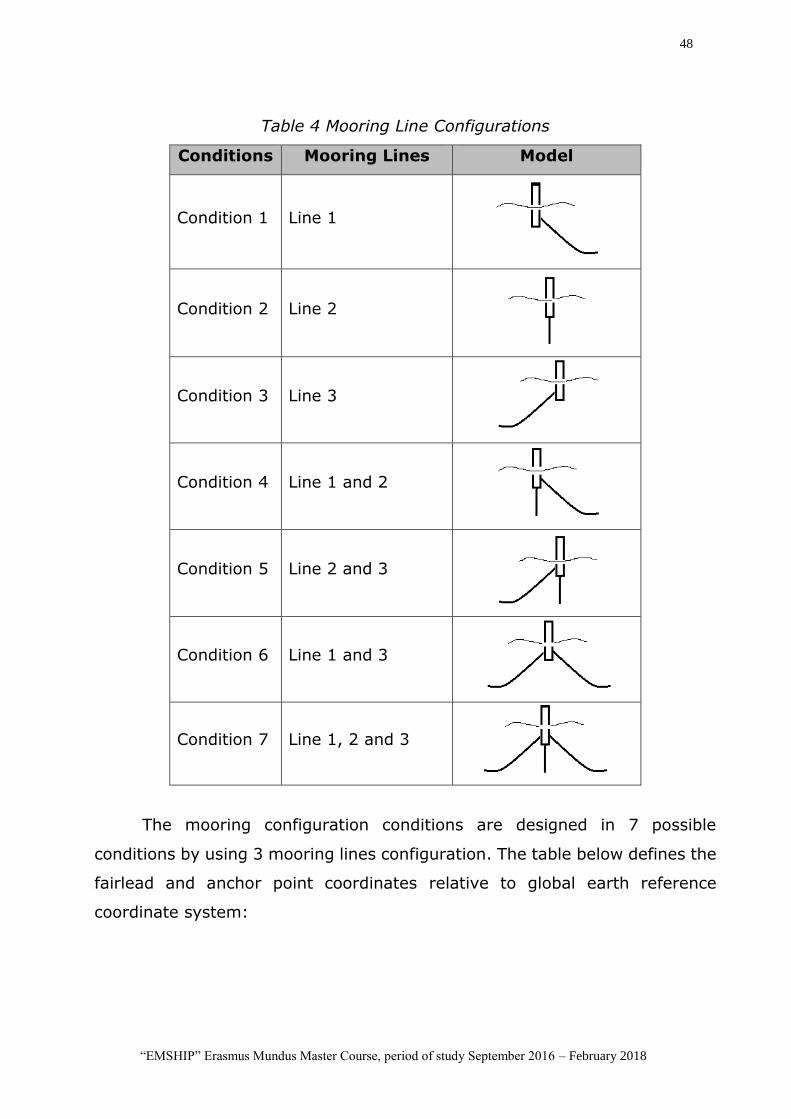
48
“EMSHIP” Erasmus Mundus Master Course, period of study September 2016 – February 2018
Table 4 Mooring Line Configurations
Conditions Mooring Lines Model
Condition 1 Line 1
Condition 2 Line 2
Condition 3 Line 3
Condition 4 Line 1 and 2
Condition 5 Line 2 and 3
Condition 6 Line 1 and 3
Condition 7 Line 1, 2 and 3
The mooring configuration conditions are designed in 7 possible
conditions by using 3 mooring lines configuration. The table below defines the
fairlead and anchor point coordinates relative to global earth reference
coordinate system:
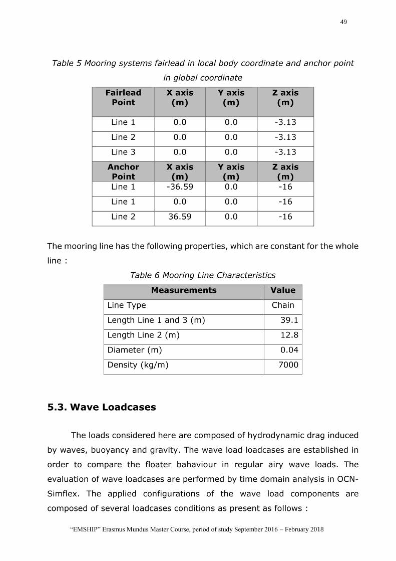
49
“EMSHIP” Erasmus Mundus Master Course, period of study September 2016 – February 2018
Table 5 Mooring systems fairlead in local body coordinate and anchor point
in global coordinate
Fairlead Point
X axis (m)
Y axis (m)
Z axis (m)
Line 1 0.0 0.0 -3.13
Line 2 0.0 0.0 -3.13
Line 3 0.0 0.0 -3.13
Anchor Point
X axis (m)
Y axis (m)
Z axis (m)
Line 1 -36.59 0.0 -16
Line 1 0.0 0.0 -16
Line 2 36.59 0.0 -16
The mooring line has the following properties, which are constant for the whole
line :
Table 6 Mooring Line Characteristics
Measurements Value
Line Type Chain
Length Line 1 and 3 (m) 39.1
Length Line 2 (m) 12.8
Diameter (m) 0.04
Density (kg/m) 7000
5.3. Wave Loadcases
The loads considered here are composed of hydrodynamic drag induced
by waves, buoyancy and gravity. The wave load loadcases are established in
order to compare the floater bahaviour in regular airy wave loads. The
evaluation of wave loadcases are performed by time domain analysis in OCN-
Simflex. The applied configurations of the wave load components are
composed of several loadcases conditions as present as follows :
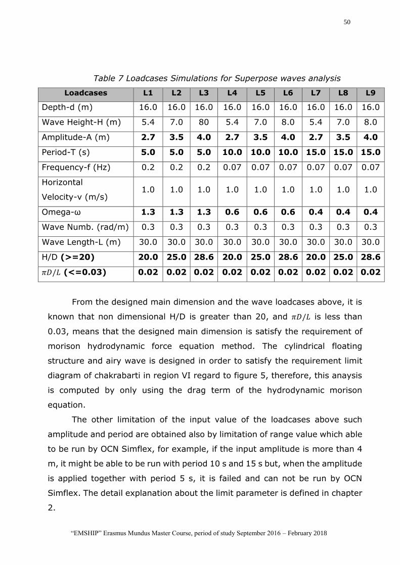
50
“EMSHIP” Erasmus Mundus Master Course, period of study September 2016 – February 2018
Table 7 Loadcases Simulations for Superpose waves analysis
Loadcases L1 L2 L3 L4 L5 L6 L7 L8 L9
Depth-d (m) 16.0 16.0 16.0 16.0 16.0 16.0 16.0 16.0 16.0
Wave Height-H (m) 5.4 7.0 80 5.4 7.0 8.0 5.4 7.0 8.0
Amplitude-A (m) 2.7 3.5 4.0 2.7 3.5 4.0 2.7 3.5 4.0
Period-T (s) 5.0 5.0 5.0 10.0 10.0 10.0 15.0 15.0 15.0
Frequency-f (Hz) 0.2 0.2 0.2 0.07 0.07 0.07 0.07 0.07 0.07
Horizontal
Velocity-v (m/s) 1.0 1.0 1.0 1.0 1.0 1.0 1.0 1.0 1.0
Omega-ω 1.3 1.3 1.3 0.6 0.6 0.6 0.4 0.4 0.4
Wave Numb. (rad/m) 0.3 0.3 0.3 0.3 0.3 0.3 0.3 0.3 0.3
Wave Length-L (m) 30.0 30.0 30.0 30.0 30.0 30.0 30.0 30.0 30.0
H/D (>=20) 20.0 25.0 28.6 20.0 25.0 28.6 20.0 25.0 28.6
𝜋𝐷/𝐿 (<=0.03) 0.02 0.02 0.02 0.02 0.02 0.02 0.02 0.02 0.02
From the designed main dimension and the wave loadcases above, it is
known that non dimensional H/D is greater than 20, and 𝜋𝐷/𝐿 is less than
0.03, means that the designed main dimension is satisfy the requirement of
morison hydrodynamic force equation method. The cylindrical floating
structure and airy wave is designed in order to satisfy the requirement limit
diagram of chakrabarti in region VI regard to figure 5, therefore, this anaysis
is computed by only using the drag term of the hydrodynamic morison
equation.
The other limitation of the input value of the loadcases above such
amplitude and period are obtained also by limitation of range value which able
to be run by OCN Simflex, for example, if the input amplitude is more than 4
m, it might be able to be run with period 10 s and 15 s but, when the amplitude
is applied together with period 5 s, it is failed and can not be run by OCN
Simflex. The detail explanation about the limit parameter is defined in chapter
2.
51
“EMSHIP” Erasmus Mundus Master Course, period of study September 2016 – February 2018
6. TIME DOMAIN ANALYSIS RESULT
The response result is computed by OCN Simflex program, while for
postprocessing result is using Paraview program. The motion response is
presented as the displacement of offset area at x and z in (+) and (-) axis .
The maximum tension of mooring line induced by Horizontal Airy wave load
configuration. There are 2 configuration of the simulation, those are
configurations of mooring line and configurations of airy wave loadcases. As
introduced earliear in section 5.3 and 5.2, the cylindrical model with mooring
line configurations are induced by horizontal airy wave loadcases. In this
section, some findings of the simulation is done and will be explained in next
part.
The results also present the draft and trim of cylindr floating structure,
in order to get more clear visualization, the draft and trim description are
described as figure 21.
6.1. Results and Comparison of Displacement Motion
Response
In order to introduce an understanding of how the airy wave loads acting
on the structure, the displacement caused by the movement of the structure
will be presented in this cahpter. The results are presented in two type, first
is the overall maximum displacement result in it’s time step. The second is
the displacement response of time step no. 73.
The first results will show the maximum probability result of
displacement response for the overall condition in all wave load cases. From
this information, it can be observed the maximum probability displacement
for each mooring design condition at each wave load case. However the
relation of displacement and wave loadcases with different wave amplitude
and period can not be observed, since the variation of the results may vary
depend on the time step of their maximum displacement in each condition and
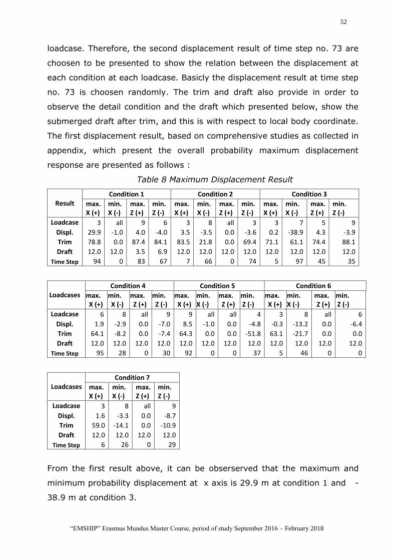
52
“EMSHIP” Erasmus Mundus Master Course, period of study September 2016 – February 2018
loadcase. Therefore, the second displacement result of time step no. 73 are
choosen to be presented to show the relation between the displacement at
each condition at each loadcase. Basicly the displacement result at time step
no. 73 is choosen randomly. The trim and draft also provide in order to
observe the detail condition and the draft which presented below, show the
submerged draft after trim, and this is with respect to local body coordinate.
The first displacement result, based on comprehensive studies as collected in
appendix, which present the overall probability maximum displacement
response are presented as follows :
Table 8 Maximum Displacement Result
Result Condition 1 Condition 2 Condition 3
max. X (+)
min. X (-)
max. Z (+)
min. Z (-)
max. X (+)
min. X (-)
max. Z (+)
min. Z (-)
max. X (+)
min. X (-)
max. Z (+)
min. Z (-)
Loadcase 3 all 9 6 3 8 all 3 3 7 5 9
Displ. 29.9 -1.0 4.0 -4.0 3.5 -3.5 0.0 -3.6 0.2 -38.9 4.3 -3.9
Trim 78.8 0.0 87.4 84.1 83.5 21.8 0.0 69.4 71.1 61.1 74.4 88.1
Draft 12.0 12.0 3.5 6.9 12.0 12.0 12.0 12.0 12.0 12.0 12.0 12.0
Time Step 94 0 83 67 7 66 0 74 5 97 45 35
Loadcases Condition 4 Condition 5 Condition 6
max. X (+)
min. X (-)
max. Z (+)
min. Z (-)
max. X (+)
min. X (-)
max. Z (+)
min. Z (-)
max. X (+)
min. X (-)
max. Z (+)
min. Z (-)
Loadcase 6 8 all 9 9 all all 4 3 8 all 6
Displ. 1.9 -2.9 0.0 -7.0 8.5 -1.0 0.0 -4.8 -0.3 -13.2 0.0 -6.4
Trim 64.1 -8.2 0.0 -7.4 64.3 0.0 0.0 -51.8 63.1 -21.7 0.0 0.0
Draft 12.0 12.0 12.0 12.0 12.0 12.0 12.0 12.0 12.0 12.0 12.0 12.0
Time Step 95 28 0 30 92 0 0 37 5 46 0 0
Loadcases Condition 7
max. X (+)
min. X (-)
max. Z (+)
min. Z (-)
Loadcase 3 8 all 9
Displ. 1.6 -3.3 0.0 -8.7
Trim 59.0 -14.1 0.0 -10.9
Draft 12.0 12.0 12.0 12.0
Time Step 6 26 0 29
From the first result above, it can be obserserved that the maximum and
minimum probability displacement at x axis is 29.9 m at condition 1 and -
38.9 m at condition 3.
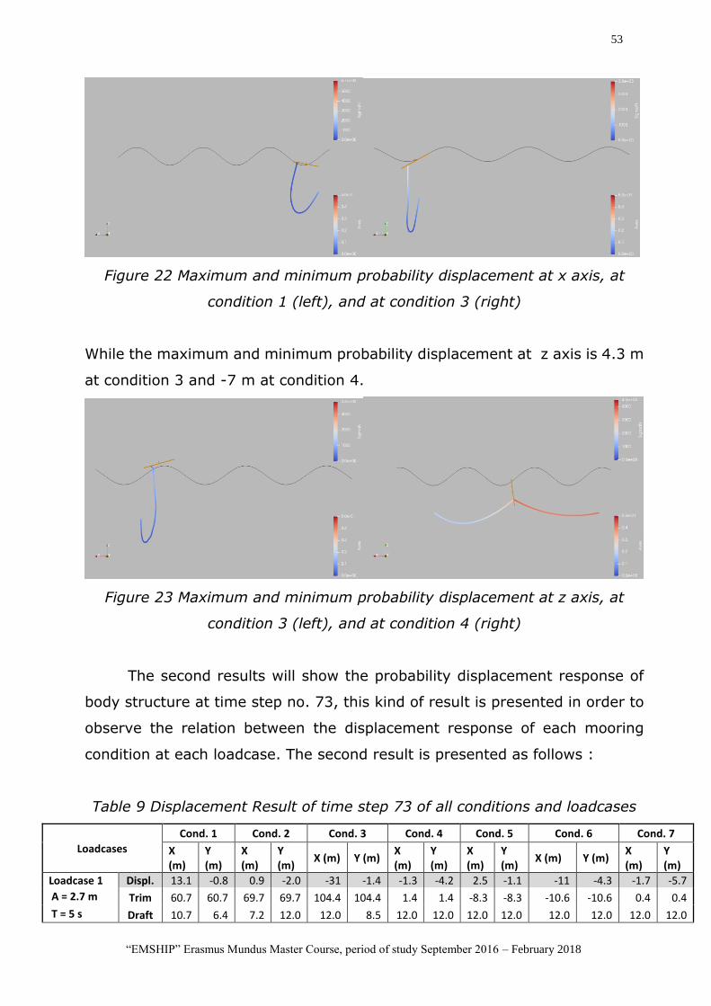
53
“EMSHIP” Erasmus Mundus Master Course, period of study September 2016 – February 2018
Figure 22 Maximum and minimum probability displacement at x axis, at
condition 1 (left), and at condition 3 (right)
While the maximum and minimum probability displacement at z axis is 4.3 m
at condition 3 and -7 m at condition 4.
Figure 23 Maximum and minimum probability displacement at z axis, at
condition 3 (left), and at condition 4 (right)
The second results will show the probability displacement response of
body structure at time step no. 73, this kind of result is presented in order to
observe the relation between the displacement response of each mooring
condition at each loadcase. The second result is presented as follows :
Table 9 Displacement Result of time step 73 of all conditions and loadcases
Loadcases
Cond. 1 Cond. 2 Cond. 3 Cond. 4 Cond. 5 Cond. 6 Cond. 7
X (m)
Y (m)
X (m)
Y (m)
X (m) Y (m) X (m)
Y (m)
X (m)
Y (m)
X (m) Y (m) X (m)
Y (m)
Loadcase 1 Displ. 13.1 -0.8 0.9 -2.0 -31 -1.4 -1.3 -4.2 2.5 -1.1 -11 -4.3 -1.7 -5.7
A = 2.7 m Trim 60.7 60.7 69.7 69.7 104.4 104.4 1.4 1.4 -8.3 -8.3 -10.6 -10.6 0.4 0.4
T = 5 s Draft 10.7 6.4 7.2 12.0 12.0 8.5 12.0 12.0 12.0 12.0 12.0 12.0 12.0 12.0
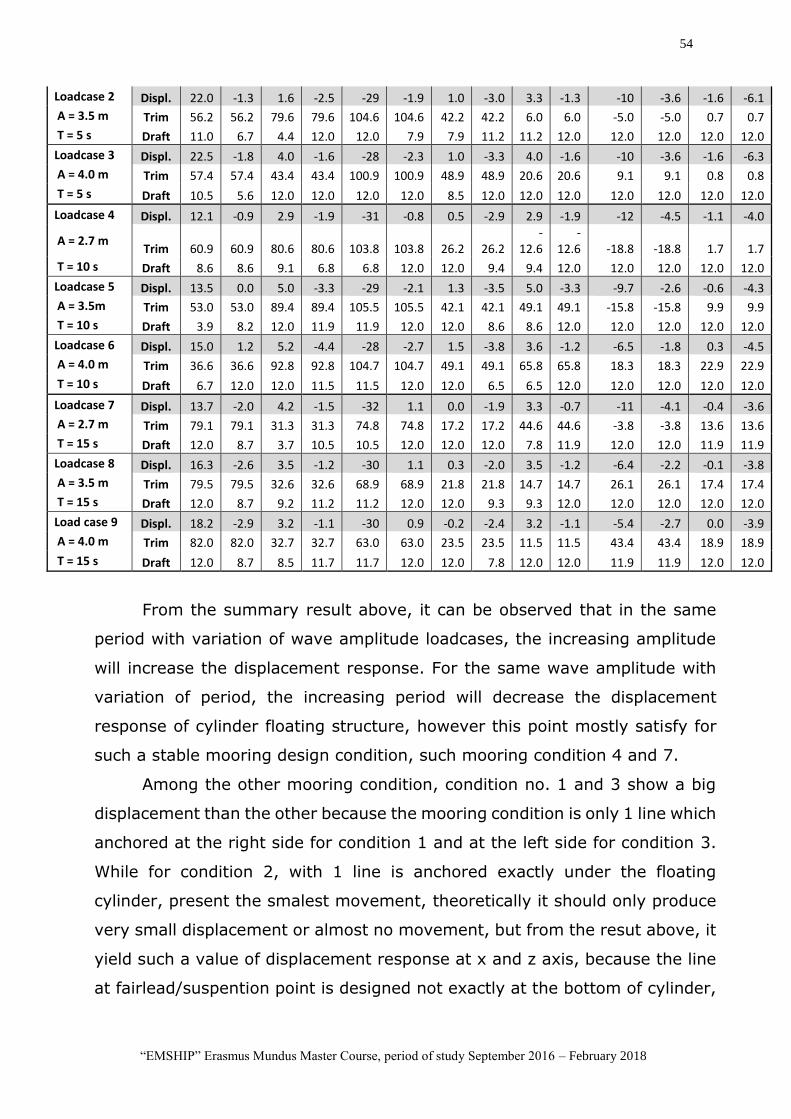
54
“EMSHIP” Erasmus Mundus Master Course, period of study September 2016 – February 2018
Loadcase 2 Displ. 22.0 -1.3 1.6 -2.5 -29 -1.9 1.0 -3.0 3.3 -1.3 -10 -3.6 -1.6 -6.1
A = 3.5 m Trim 56.2 56.2 79.6 79.6 104.6 104.6 42.2 42.2 6.0 6.0 -5.0 -5.0 0.7 0.7
T = 5 s Draft 11.0 6.7 4.4 12.0 12.0 7.9 7.9 11.2 11.2 12.0 12.0 12.0 12.0 12.0
Loadcase 3 Displ. 22.5 -1.8 4.0 -1.6 -28 -2.3 1.0 -3.3 4.0 -1.6 -10 -3.6 -1.6 -6.3
A = 4.0 m Trim 57.4 57.4 43.4 43.4 100.9 100.9 48.9 48.9 20.6 20.6 9.1 9.1 0.8 0.8
T = 5 s Draft 10.5 5.6 12.0 12.0 12.0 12.0 8.5 12.0 12.0 12.0 12.0 12.0 12.0 12.0
Loadcase 4 Displ. 12.1 -0.9 2.9 -1.9 -31 -0.8 0.5 -2.9 2.9 -1.9 -12 -4.5 -1.1 -4.0
A = 2.7 m Trim 60.9 60.9 80.6 80.6 103.8 103.8 26.2 26.2
-12.6
-12.6 -18.8 -18.8 1.7 1.7
T = 10 s Draft 8.6 8.6 9.1 6.8 6.8 12.0 12.0 9.4 9.4 12.0 12.0 12.0 12.0 12.0
Loadcase 5 Displ. 13.5 0.0 5.0 -3.3 -29 -2.1 1.3 -3.5 5.0 -3.3 -9.7 -2.6 -0.6 -4.3
A = 3.5m Trim 53.0 53.0 89.4 89.4 105.5 105.5 42.1 42.1 49.1 49.1 -15.8 -15.8 9.9 9.9
T = 10 s Draft 3.9 8.2 12.0 11.9 11.9 12.0 12.0 8.6 8.6 12.0 12.0 12.0 12.0 12.0
Loadcase 6 Displ. 15.0 1.2 5.2 -4.4 -28 -2.7 1.5 -3.8 3.6 -1.2 -6.5 -1.8 0.3 -4.5
A = 4.0 m Trim 36.6 36.6 92.8 92.8 104.7 104.7 49.1 49.1 65.8 65.8 18.3 18.3 22.9 22.9
T = 10 s Draft 6.7 12.0 12.0 11.5 11.5 12.0 12.0 6.5 6.5 12.0 12.0 12.0 12.0 12.0
Loadcase 7 Displ. 13.7 -2.0 4.2 -1.5 -32 1.1 0.0 -1.9 3.3 -0.7 -11 -4.1 -0.4 -3.6
A = 2.7 m Trim 79.1 79.1 31.3 31.3 74.8 74.8 17.2 17.2 44.6 44.6 -3.8 -3.8 13.6 13.6
T = 15 s Draft 12.0 8.7 3.7 10.5 10.5 12.0 12.0 12.0 7.8 11.9 12.0 12.0 11.9 11.9
Loadcase 8 Displ. 16.3 -2.6 3.5 -1.2 -30 1.1 0.3 -2.0 3.5 -1.2 -6.4 -2.2 -0.1 -3.8
A = 3.5 m Trim 79.5 79.5 32.6 32.6 68.9 68.9 21.8 21.8 14.7 14.7 26.1 26.1 17.4 17.4
T = 15 s Draft 12.0 8.7 9.2 11.2 11.2 12.0 12.0 9.3 9.3 12.0 12.0 12.0 12.0 12.0
Load case 9 Displ. 18.2 -2.9 3.2 -1.1 -30 0.9 -0.2 -2.4 3.2 -1.1 -5.4 -2.7 0.0 -3.9
A = 4.0 m Trim 82.0 82.0 32.7 32.7 63.0 63.0 23.5 23.5 11.5 11.5 43.4 43.4 18.9 18.9
T = 15 s Draft 12.0 8.7 8.5 11.7 11.7 12.0 12.0 7.8 12.0 12.0 11.9 11.9 12.0 12.0
From the summary result above, it can be observed that in the same
period with variation of wave amplitude loadcases, the increasing amplitude
will increase the displacement response. For the same wave amplitude with
variation of period, the increasing period will decrease the displacement
response of cylinder floating structure, however this point mostly satisfy for
such a stable mooring design condition, such mooring condition 4 and 7.
Among the other mooring condition, condition no. 1 and 3 show a big
displacement than the other because the mooring condition is only 1 line which
anchored at the right side for condition 1 and at the left side for condition 3.
While for condition 2, with 1 line is anchored exactly under the floating
cylinder, present the smalest movement, theoretically it should only produce
very small displacement or almost no movement, but from the resut above, it
yield such a value of displacement response at x and z axis, because the line
at fairlead/suspention point is designed not exactly at the bottom of cylinder,
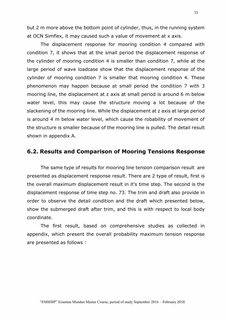
55
“EMSHIP” Erasmus Mundus Master Course, period of study September 2016 – February 2018
but 2 m more above the bottom point of cylinder, thus, in the running system
at OCN Simflex, it may caused such a value of movement at x axis.
The displacement response for mooring condition 4 compared with
condition 7, it shows that at the small period the displacement response of
the cylinder of mooring condition 4 is smaller than condition 7, while at the
large period of wave loadcase show that the displacement response of the
cylinder of mooring condition 7 is smaller that mooring condition 4. These
phenomenon may happen because at small period the condition 7 with 3
mooring line, the displacement at z axis at small period is around 6 m below
water level, this may cause the structure moving a lot because of the
slackening of the mooring line. While the displacement at z axis at large period
is around 4 m below water level, which cause the robability of movement of
the structure is smaller because of the mooring line is pulled. The detail result
shown in appendix A.
6.2. Results and Comparison of Mooring Tensions Response
The same type of results for mooring line tension comparison result are
presented as displacement response result. There are 2 type of result, first is
the overall maximum displacement result in it’s time step. The second is the
displacement response of time step no. 73. The trim and draft also provide in
order to observe the detail condition and the draft which presented below,
show the submerged draft after trim, and this is with respect to local body
coordinate.
The first result, based on comprehensive studies as collected in
appendix, which present the overall probability maximum tension response
are presented as follows :
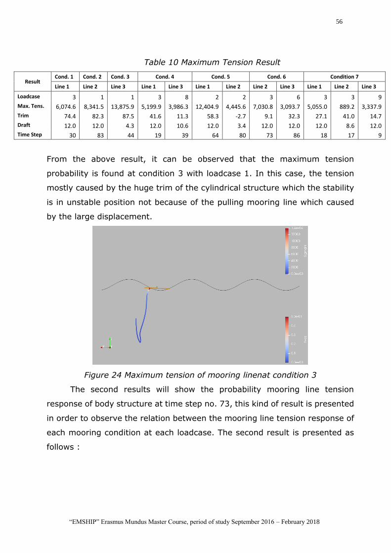
56
“EMSHIP” Erasmus Mundus Master Course, period of study September 2016 – February 2018
Table 10 Maximum Tension Result
Result Cond. 1 Cond. 2 Cond. 3 Cond. 4 Cond. 5 Cond. 6 Condition 7
Line 1 Line 2 Line 3 Line 1 Line 3 Line 1 Line 2 Line 2 Line 3 Line 1 Line 2 Line 3
Loadcase 3 1 1 3 8 2 2 3 6 3 3 9
Max. Tens. 6,074.6 8,341.5 13,875.9 5,199.9 3,986.3 12,404.9 4,445.6 7,030.8 3,093.7 5,055.0 889.2 3,337.9
Trim 74.4 82.3 87.5 41.6 11.3 58.3 -2.7 9.1 32.3 27.1 41.0 14.7
Draft 12.0 12.0 4.3 12.0 10.6 12.0 3.4 12.0 12.0 12.0 8.6 12.0
Time Step 30 83 44 19 39 64 80 73 86 18 17 9
From the above result, it can be observed that the maximum tension
probability is found at condition 3 with loadcase 1. In this case, the tension
mostly caused by the huge trim of the cylindrical structure which the stability
is in unstable position not because of the pulling mooring line which caused
by the large displacement.
Figure 24 Maximum tension of mooring linenat condition 3
The second results will show the probability mooring line tension
response of body structure at time step no. 73, this kind of result is presented
in order to observe the relation between the mooring line tension response of
each mooring condition at each loadcase. The second result is presented as
follows :
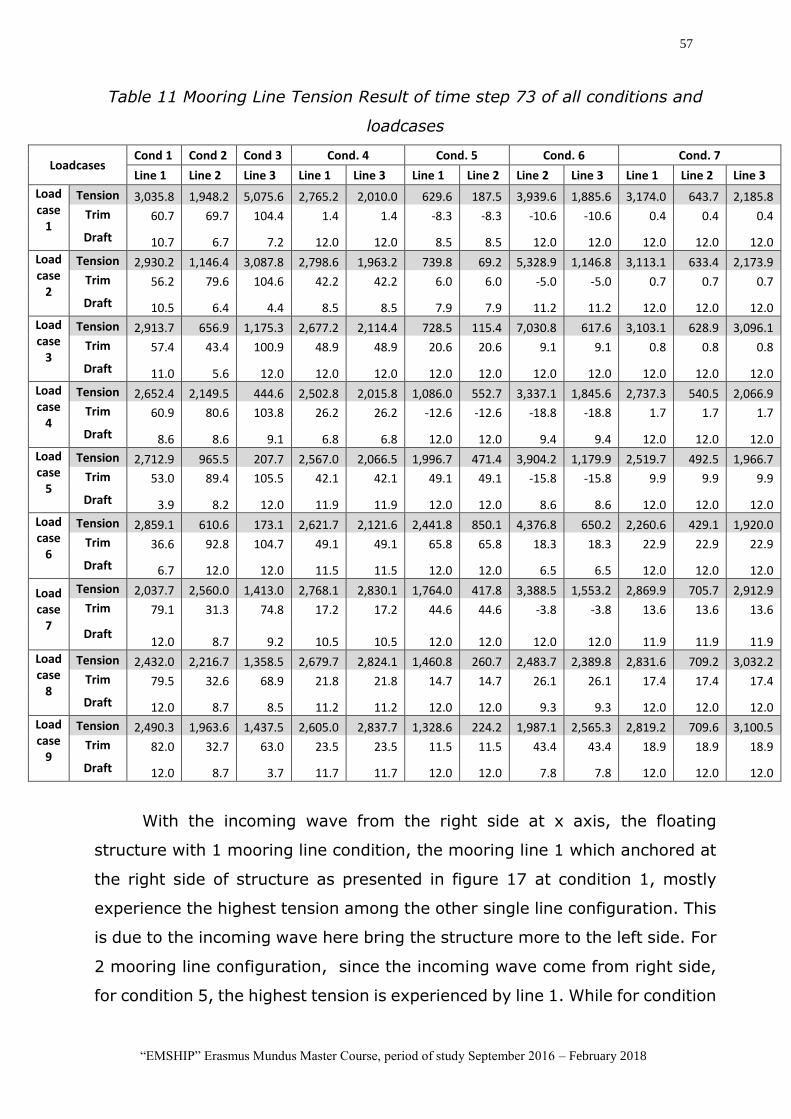
57
“EMSHIP” Erasmus Mundus Master Course, period of study September 2016 – February 2018
Table 11 Mooring Line Tension Result of time step 73 of all conditions and
loadcases
Loadcases Cond 1 Cond 2 Cond 3 Cond. 4 Cond. 5 Cond. 6 Cond. 7
Line 1 Line 2 Line 3 Line 1 Line 3 Line 1 Line 2 Line 2 Line 3 Line 1 Line 2 Line 3
Load case
1
Tension 3,035.8 1,948.2 5,075.6 2,765.2 2,010.0 629.6 187.5 3,939.6 1,885.6 3,174.0 643.7 2,185.8
Trim 60.7 69.7 104.4 1.4 1.4 -8.3 -8.3 -10.6 -10.6 0.4 0.4 0.4
Draft 10.7 6.7 7.2 12.0 12.0 8.5 8.5 12.0 12.0 12.0 12.0 12.0
Load case
2
Tension 2,930.2 1,146.4 3,087.8 2,798.6 1,963.2 739.8 69.2 5,328.9 1,146.8 3,113.1 633.4 2,173.9
Trim 56.2 79.6 104.6 42.2 42.2 6.0 6.0 -5.0 -5.0 0.7 0.7 0.7
Draft 10.5 6.4 4.4 8.5 8.5 7.9 7.9 11.2 11.2 12.0 12.0 12.0
Load case
3
Tension 2,913.7 656.9 1,175.3 2,677.2 2,114.4 728.5 115.4 7,030.8 617.6 3,103.1 628.9 3,096.1
Trim 57.4 43.4 100.9 48.9 48.9 20.6 20.6 9.1 9.1 0.8 0.8 0.8
Draft 11.0 5.6 12.0 12.0 12.0 12.0 12.0 12.0 12.0 12.0 12.0 12.0
Load case
4
Tension 2,652.4 2,149.5 444.6 2,502.8 2,015.8 1,086.0 552.7 3,337.1 1,845.6 2,737.3 540.5 2,066.9
Trim 60.9 80.6 103.8 26.2 26.2 -12.6 -12.6 -18.8 -18.8 1.7 1.7 1.7
Draft 8.6 8.6 9.1 6.8 6.8 12.0 12.0 9.4 9.4 12.0 12.0 12.0
Load case
5
Tension 2,712.9 965.5 207.7 2,567.0 2,066.5 1,996.7 471.4 3,904.2 1,179.9 2,519.7 492.5 1,966.7
Trim 53.0 89.4 105.5 42.1 42.1 49.1 49.1 -15.8 -15.8 9.9 9.9 9.9
Draft 3.9 8.2 12.0 11.9 11.9 12.0 12.0 8.6 8.6 12.0 12.0 12.0
Load case
6
Tension 2,859.1 610.6 173.1 2,621.7 2,121.6 2,441.8 850.1 4,376.8 650.2 2,260.6 429.1 1,920.0
Trim 36.6 92.8 104.7 49.1 49.1 65.8 65.8 18.3 18.3 22.9 22.9 22.9
Draft 6.7 12.0 12.0 11.5 11.5 12.0 12.0 6.5 6.5 12.0 12.0 12.0
Load case
7
Tension 2,037.7 2,560.0 1,413.0 2,768.1 2,830.1 1,764.0 417.8 3,388.5 1,553.2 2,869.9 705.7 2,912.9
Trim 79.1 31.3 74.8 17.2 17.2 44.6 44.6 -3.8 -3.8 13.6 13.6 13.6
Draft 12.0 8.7 9.2 10.5 10.5 12.0 12.0 12.0 12.0 11.9 11.9 11.9
Load case
8
Tension 2,432.0 2,216.7 1,358.5 2,679.7 2,824.1 1,460.8 260.7 2,483.7 2,389.8 2,831.6 709.2 3,032.2
Trim 79.5 32.6 68.9 21.8 21.8 14.7 14.7 26.1 26.1 17.4 17.4 17.4
Draft 12.0 8.7 8.5 11.2 11.2 12.0 12.0 9.3 9.3 12.0 12.0 12.0
Load case
9
Tension 2,490.3 1,963.6 1,437.5 2,605.0 2,837.7 1,328.6 224.2 1,987.1 2,565.3 2,819.2 709.6 3,100.5
Trim 82.0 32.7 63.0 23.5 23.5 11.5 11.5 43.4 43.4 18.9 18.9 18.9
Draft 12.0 8.7 3.7 11.7 11.7 12.0 12.0 7.8 7.8 12.0 12.0 12.0
With the incoming wave from the right side at x axis, the floating
structure with 1 mooring line condition, the mooring line 1 which anchored at
the right side of structure as presented in figure 17 at condition 1, mostly
experience the highest tension among the other single line configuration. This
is due to the incoming wave here bring the structure more to the left side. For
2 mooring line configuration, since the incoming wave come from right side,
for condition 5, the highest tension is experienced by line 1. While for condition
58
“EMSHIP” Erasmus Mundus Master Course, period of study September 2016 – February 2018
6, the highest tension is experienced by line 2 at all loadcases. For condition
4 with 2 line configuration at both side right and left is compared with condition
7 with the same configuration and 1 additional mooring line exactly under the
floating structure. The highest tension is experienced by line 1 for both
condition, but only for loadcase 1 to 6 with period 5 s and 10 s. While for
loadcase 7 to 9 with higher period 15 s, the highest tension is experienced by
line 3. This is because the loadcase with small period, bring the structure
mostly going to the right side, while with large period, bring the structure
mostly going to the left side because the process become slower. However,
the highest tension at line 1 in condition 7 is higher than in condition 4. This
is because line 1 should taking into account the appearance of line 2 at
condition 7, which bring the effect of it’s weight, where the line 2 here is in
slackening position also. Taking such a sample result from condition 4 and 7
ay laodcase 7, 8 and 9 also show that the decreasing trim of line 1 yield to
the increasing tension of line 1. The detail result shown in appendix A.
6.3. Results and Comparison of Stability
The results for mooring line stability response comparison result are
presented as the stability response of time step no. 73, which is choosen
randomly. All results are presented in the same time step in order to present
the relation between the stability response at each condition and loadcase at
same time step. Fg is gravity force and Fb is buoyancy force. The stability
results at below table provide the buoyancy and gravity force in order to
present the comparison study of the trim angle response of structure at each
condition and loadcase. The drafts in table below are presented as the draft
before trim response of cylinder structure.
Table 12 Stability Result of time step 73 of all conditions and Loadcases
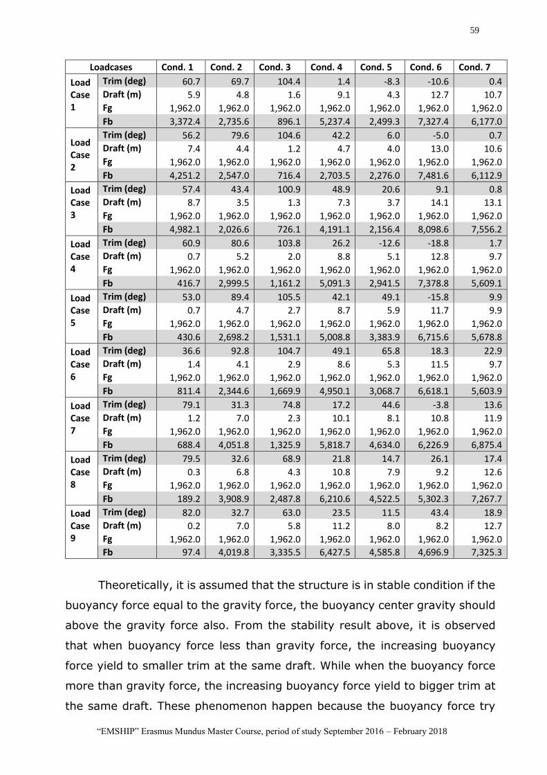
59
“EMSHIP” Erasmus Mundus Master Course, period of study September 2016 – February 2018
Loadcases Cond. 1 Cond. 2 Cond. 3 Cond. 4 Cond. 5 Cond. 6 Cond. 7
Load Case 1
Trim (deg) 60.7 69.7 104.4 1.4 -8.3 -10.6 0.4
Draft (m) 5.9 4.8 1.6 9.1 4.3 12.7 10.7
Fg 1,962.0 1,962.0 1,962.0 1,962.0 1,962.0 1,962.0 1,962.0
Fb 3,372.4 2,735.6 896.1 5,237.4 2,499.3 7,327.4 6,177.0
Load Case 2
Trim (deg) 56.2 79.6 104.6 42.2 6.0 -5.0 0.7
Draft (m) 7.4 4.4 1.2 4.7 4.0 13.0 10.6
Fg 1,962.0 1,962.0 1,962.0 1,962.0 1,962.0 1,962.0 1,962.0
Fb 4,251.2 2,547.0 716.4 2,703.5 2,276.0 7,481.6 6,112.9
Load Case 3
Trim (deg) 57.4 43.4 100.9 48.9 20.6 9.1 0.8
Draft (m) 8.7 3.5 1.3 7.3 3.7 14.1 13.1
Fg 1,962.0 1,962.0 1,962.0 1,962.0 1,962.0 1,962.0 1,962.0
Fb 4,982.1 2,026.6 726.1 4,191.1 2,156.4 8,098.6 7,556.2
Load Case 4
Trim (deg) 60.9 80.6 103.8 26.2 -12.6 -18.8 1.7
Draft (m) 0.7 5.2 2.0 8.8 5.1 12.8 9.7
Fg 1,962.0 1,962.0 1,962.0 1,962.0 1,962.0 1,962.0 1,962.0
Fb 416.7 2,999.5 1,161.2 5,091.3 2,941.5 7,378.8 5,609.1
Load Case 5
Trim (deg) 53.0 89.4 105.5 42.1 49.1 -15.8 9.9
Draft (m) 0.7 4.7 2.7 8.7 5.9 11.7 9.9
Fg 1,962.0 1,962.0 1,962.0 1,962.0 1,962.0 1,962.0 1,962.0
Fb 430.6 2,698.2 1,531.1 5,008.8 3,383.9 6,715.6 5,678.8
Load Case 6
Trim (deg) 36.6 92.8 104.7 49.1 65.8 18.3 22.9
Draft (m) 1.4 4.1 2.9 8.6 5.3 11.5 9.7
Fg 1,962.0 1,962.0 1,962.0 1,962.0 1,962.0 1,962.0 1,962.0
Fb 811.4 2,344.6 1,669.9 4,950.1 3,068.7 6,618.1 5,603.9
Load Case 7
Trim (deg) 79.1 31.3 74.8 17.2 44.6 -3.8 13.6
Draft (m) 1.2 7.0 2.3 10.1 8.1 10.8 11.9
Fg 1,962.0 1,962.0 1,962.0 1,962.0 1,962.0 1,962.0 1,962.0
Fb 688.4 4,051.8 1,325.9 5,818.7 4,634.0 6,226.9 6,875.4
Load Case 8
Trim (deg) 79.5 32.6 68.9 21.8 14.7 26.1 17.4
Draft (m) 0.3 6.8 4.3 10.8 7.9 9.2 12.6
Fg 1,962.0 1,962.0 1,962.0 1,962.0 1,962.0 1,962.0 1,962.0
Fb 189.2 3,908.9 2,487.8 6,210.6 4,522.5 5,302.3 7,267.7
Load Case 9
Trim (deg) 82.0 32.7 63.0 23.5 11.5 43.4 18.9
Draft (m) 0.2 7.0 5.8 11.2 8.0 8.2 12.7
Fg 1,962.0 1,962.0 1,962.0 1,962.0 1,962.0 1,962.0 1,962.0
Fb 97.4 4,019.8 3,335.5 6,427.5 4,585.8 4,696.9 7,325.3
Theoretically, it is assumed that the structure is in stable condition if the
buoyancy force equal to the gravity force, the buoyancy center gravity should
above the gravity force also. From the stability result above, it is observed
that when buoyancy force less than gravity force, the increasing buoyancy
force yield to smaller trim at the same draft. While when the buoyancy force
more than gravity force, the increasing buoyancy force yield to bigger trim at
the same draft. These phenomenon happen because the buoyancy force try
60
“EMSHIP” Erasmus Mundus Master Course, period of study September 2016 – February 2018
to achieve the same value of gravity force to get a stable condition by the trim
of the floating body it self.
For the condition with 1 mooring line, such condition 1 ,2 and 3, the
condition 3 at period 5 s and 10 s, show the unstable result, therefore it yield
to largest trim among the other condition. While the condition 3 at loadcases
with period 15 s, the conditions is more stable and at these period, condition
2 show the smallest trim. For condition 4 with 2 mooring line at both side
compare with condition 7 with the same condition and additional mooring line
at the center, the larger draft of condition 7, yield to smaller trim angle than
condition 4.
61
“EMSHIP” Erasmus Mundus Master Course, period of study September 2016 – February 2018
7. CONCLUSION AND FURTHER STUDIES
7.1. Conclusions
The hydrodynamic interaction effect and dynamic response are the
major consideration in the design of floating structures. The hydrodynamic
load calculation is necessary to be obtained in order to analyze the response.
A set of morison hydrodynamic algorithm is used and presented by Matlab
program, the morison hydrodynamic computation method is selected because
of the shape of floating structure considered as slender transparant structure.
The set of algorithm in Matlab is to test the plausibility of the developed
algorithm and to be used as reference documentation for deeper
understanding for author and other researcher also.
A sample model of cylinder transparent structure and wave loadcases
are designed in order to satisfy the region VI of diagram chakrabarti. This
model is used in order to execute the comparative study of floating structure
response induced by horizontal airy wave using hydrodynamic morison
method.
From the comparative study of the response result, it can be assumed
that, in the same period with variation of wave amplitude loadcases, the
increasing amplitude will increase the displacement response. For the same
wave amplitude with variation of period, the increasing period will decrease
the displacement response of cylinder floating structure. Regarding the
mooring line tension, the line tension 1 increase when the trim and draft
before trim of strucure decrease, and the largest tension will be observed at
the mooring line which anchored at same direction with the incoming wave.
Regarding the stability, when buoyancy force less than gravity force, the
increasing buoyancy force yield to smaller trim at the same draft. While when
the buoyancy force more than gravity force, the increasing buoyancy force
yield to bigger trim at the same draft. These phenomenon happen because
the buoyancy force try to achieve the equal value of gravity force to get a
stable condition by the trim of the floating body it self. For condition 4 with 2
62
“EMSHIP” Erasmus Mundus Master Course, period of study September 2016 – February 2018
mooring line at both side compare with condition 7 with the same condition
and additional mooring line at the center, the larger draft of condition 7, yield
to smaller trim angle than condition 4. Means that, the addtional mooring line
at center and exactly positioned under the structure, will yield to more stable
effect for the floating cylindrical structure.
7.2. Further Studies
Further studies are needed to study the response of cylinder floating structure
as follows :
Comparison of motion response result using more than one program as
evaluation
Study the used of morison equation in large floating structure
hydroynamic load calculation and also by using fast fourier transform in
order to combine the hydrodynamic load equation in frequency domain.
63
“EMSHIP” Erasmus Mundus Master Course, period of study September 2016 – February 2018
8. ACKNOWLEDGEMENTS
Acknowledgements may be made to those individuals or institutions not
mentioned elsewhere in the thesis that made an important contribution.
Following acknowledgement must be included in this section:
This thesis was developed in the frame of the European Master Course in
“Integrated Advanced Ship Design” named “EMSHIP” for “European Education
in Advanced Ship Design”, Ref.: 159652-1-2009-1-BE-ERA MUNDUS-EMMC.
64
“EMSHIP” Erasmus Mundus Master Course, period of study September 2016 – February 2018
9. REFERENCES
Chakrabarti, S. (2010): “Handbook of Coastal and Ocean Engineering”,
edited by Young C Kim, Section 24 Offshore Structure, World Scientific Publishing Co. Pte. Ltd., Singapore.
Chakrabarti, S. (2005): “Handbook of Offshore Engineering”, edited by
Subrata Chakrabarti, Volume 1, Elsevier, Oxford, UK.
Chaudhury, G. and Yo Ho, C. (2000):”Coupled Dynamic Analysis of Platforms, Riser and Moorings”, Offshore Technology Conference, 12084 MS,
May 1‐4, Houston, Texas, USA.
Det Norske Veritas (2010): “Global Performance Analysis of Deepwater
Floating Structures”, Recommended Practice, DNV‐RP‐F205, October 2010.
Faltinsen, O. M. (1990): “Sea Loads on Ships and Offshore Structures”,
Cambridge University Press, USA‐Australia
Gudmestad, O. T. (2010): Marine Technology and Design Compendium.
University of Stavanger, Stavanger, Norway.
Journée, J. M. J. and Massie, W. W. (2001): “Offshore Hydromechanics”, First Edition, Delft University of Technology, http://www.shipmotions.nl.,
(Delft University course material).
Løken, A. E., Sødahl, N., Hagen, O., DNV (1999): ”Efficient Integrated
Analysis methods for Deepwater Platforms”, OTC 10809, Offshore Technology Conference, OTC 10809, May 3‐6, Houston, Texas, USA.
Newman, J. N. (1986): “Marine Hydrodynamics”, The Massachusetts
Institute of Technology, Cambridge, USA.
Omberg, H. and Larsen, K. (1998): “Coupled Analysis of Floater Motion
and Moorings Dynamics for a Turret‐Moored Ship”, Appl Ocean Res. (1998),
Vol 20, pp.55‐67, 8th International Conference on the Behaviour of Off‐Shore
Structure (BOSS’97), Delft, Netherlands.
Otto, Christoph.(2017): “OCN-SIMFLEX User Manual”, Rostock,Germany
Shabana, Ahmed A.(2005): “Third Edition Dynamics of Multibody Systems”,
Cambrdge University Press (2005), Universuty of Illinois, Chicago
Desmond, Cian et al(2016): “Description of an 8 MW reference wind
turbine”, journal of Physics:conference Series.
JONKMAN, J.: Definition of the Floating System for Phase IV of OC3.
Technical Report, NREL, 2010.
65
“EMSHIP” Erasmus Mundus Master Course, period of study September 2016 – February 2018
J. JONKMAN, S. BUTTERFIELD, W. MUSIAL and G. SCOTT: Definition of
a 5-MW Reference Wind Turbine for Offshore System Development. Technical Report, NREL, 2009.
Hall, Matthew Thomas Jair.(2013): Mooring Line Modelling and Design
Oprimization of Floating Offshore Wind Turbines, Master of Aplied Science in the Department of Mechanical Engineerig, University of Victoria
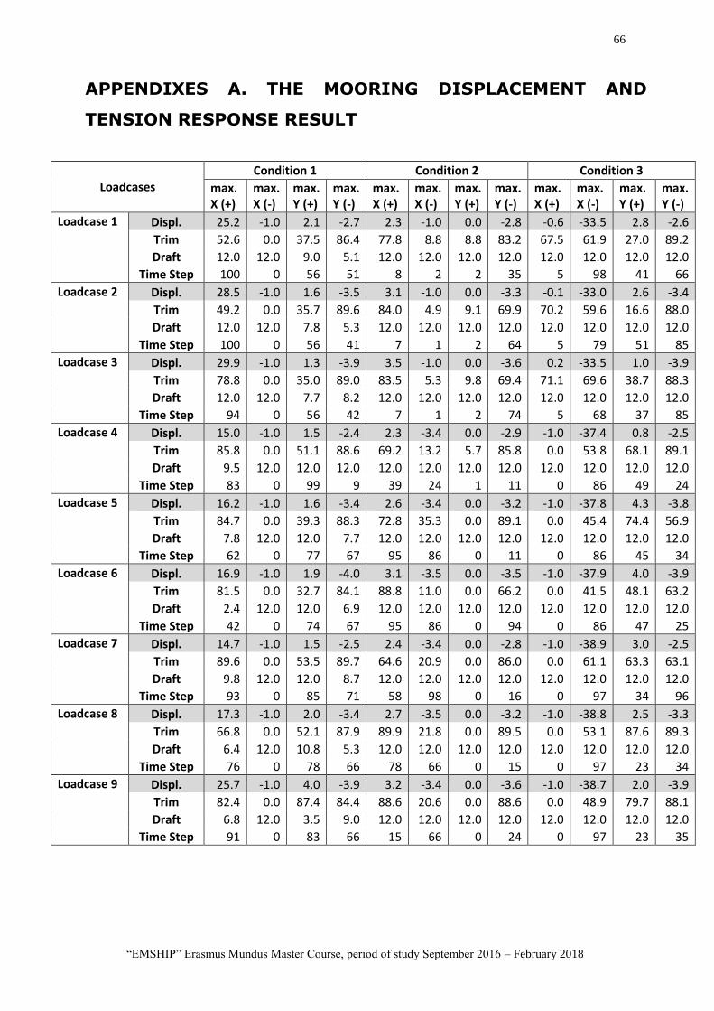
66
“EMSHIP” Erasmus Mundus Master Course, period of study September 2016 – February 2018
APPENDIXES A. THE MOORING DISPLACEMENT AND
TENSION RESPONSE RESULT
Loadcases Condition 1 Condition 2 Condition 3
max. X (+)
max. X (-)
max. Y (+)
max. Y (-)
max. X (+)
max. X (-)
max. Y (+)
max. Y (-)
max. X (+)
max. X (-)
max. Y (+)
max. Y (-)
Loadcase 1 Displ. 25.2 -1.0 2.1 -2.7 2.3 -1.0 0.0 -2.8 -0.6 -33.5 2.8 -2.6
Trim 52.6 0.0 37.5 86.4 77.8 8.8 8.8 83.2 67.5 61.9 27.0 89.2
Draft 12.0 12.0 9.0 5.1 12.0 12.0 12.0 12.0 12.0 12.0 12.0 12.0
Time Step 100 0 56 51 8 2 2 35 5 98 41 66
Loadcase 2 Displ. 28.5 -1.0 1.6 -3.5 3.1 -1.0 0.0 -3.3 -0.1 -33.0 2.6 -3.4
Trim 49.2 0.0 35.7 89.6 84.0 4.9 9.1 69.9 70.2 59.6 16.6 88.0
Draft 12.0 12.0 7.8 5.3 12.0 12.0 12.0 12.0 12.0 12.0 12.0 12.0
Time Step 100 0 56 41 7 1 2 64 5 79 51 85
Loadcase 3 Displ. 29.9 -1.0 1.3 -3.9 3.5 -1.0 0.0 -3.6 0.2 -33.5 1.0 -3.9
Trim 78.8 0.0 35.0 89.0 83.5 5.3 9.8 69.4 71.1 69.6 38.7 88.3
Draft 12.0 12.0 7.7 8.2 12.0 12.0 12.0 12.0 12.0 12.0 12.0 12.0
Time Step 94 0 56 42 7 1 2 74 5 68 37 85
Loadcase 4 Displ. 15.0 -1.0 1.5 -2.4 2.3 -3.4 0.0 -2.9 -1.0 -37.4 0.8 -2.5
Trim 85.8 0.0 51.1 88.6 69.2 13.2 5.7 85.8 0.0 53.8 68.1 89.1
Draft 9.5 12.0 12.0 12.0 12.0 12.0 12.0 12.0 12.0 12.0 12.0 12.0
Time Step 83 0 99 9 39 24 1 11 0 86 49 24
Loadcase 5 Displ. 16.2 -1.0 1.6 -3.4 2.6 -3.4 0.0 -3.2 -1.0 -37.8 4.3 -3.8
Trim 84.7 0.0 39.3 88.3 72.8 35.3 0.0 89.1 0.0 45.4 74.4 56.9
Draft 7.8 12.0 12.0 7.7 12.0 12.0 12.0 12.0 12.0 12.0 12.0 12.0
Time Step 62 0 77 67 95 86 0 11 0 86 45 34
Loadcase 6 Displ. 16.9 -1.0 1.9 -4.0 3.1 -3.5 0.0 -3.5 -1.0 -37.9 4.0 -3.9
Trim 81.5 0.0 32.7 84.1 88.8 11.0 0.0 66.2 0.0 41.5 48.1 63.2
Draft 2.4 12.0 12.0 6.9 12.0 12.0 12.0 12.0 12.0 12.0 12.0 12.0
Time Step 42 0 74 67 95 86 0 94 0 86 47 25
Loadcase 7 Displ. 14.7 -1.0 1.5 -2.5 2.4 -3.4 0.0 -2.8 -1.0 -38.9 3.0 -2.5
Trim 89.6 0.0 53.5 89.7 64.6 20.9 0.0 86.0 0.0 61.1 63.3 63.1
Draft 9.8 12.0 12.0 8.7 12.0 12.0 12.0 12.0 12.0 12.0 12.0 12.0
Time Step 93 0 85 71 58 98 0 16 0 97 34 96
Loadcase 8 Displ. 17.3 -1.0 2.0 -3.4 2.7 -3.5 0.0 -3.2 -1.0 -38.8 2.5 -3.3
Trim 66.8 0.0 52.1 87.9 89.9 21.8 0.0 89.5 0.0 53.1 87.6 89.3
Draft 6.4 12.0 10.8 5.3 12.0 12.0 12.0 12.0 12.0 12.0 12.0 12.0
Time Step 76 0 78 66 78 66 0 15 0 97 23 34
Loadcase 9 Displ. 25.7 -1.0 4.0 -3.9 3.2 -3.4 0.0 -3.6 -1.0 -38.7 2.0 -3.9
Trim 82.4 0.0 87.4 84.4 88.6 20.6 0.0 88.6 0.0 48.9 79.7 88.1
Draft 6.8 12.0 3.5 9.0 12.0 12.0 12.0 12.0 12.0 12.0 12.0 12.0
Time Step 91 0 83 66 15 66 0 24 0 97 23 35
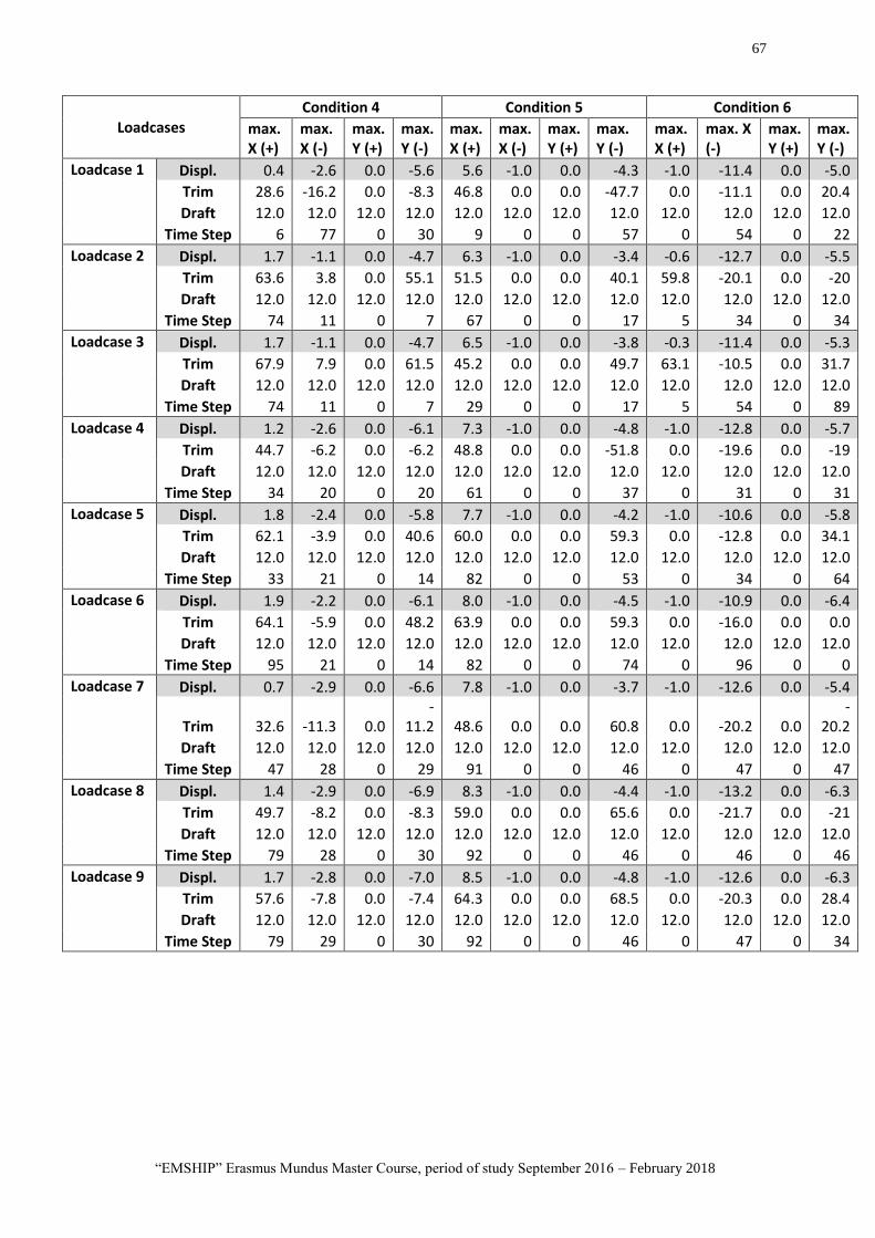
67
“EMSHIP” Erasmus Mundus Master Course, period of study September 2016 – February 2018
Loadcases Condition 4 Condition 5 Condition 6
max. X (+)
max. X (-)
max. Y (+)
max. Y (-)
max. X (+)
max. X (-)
max. Y (+)
max. Y (-)
max. X (+)
max. X (-)
max. Y (+)
max. Y (-)
Loadcase 1 Displ. 0.4 -2.6 0.0 -5.6 5.6 -1.0 0.0 -4.3 -1.0 -11.4 0.0 -5.0
Trim 28.6 -16.2 0.0 -8.3 46.8 0.0 0.0 -47.7 0.0 -11.1 0.0 20.4
Draft 12.0 12.0 12.0 12.0 12.0 12.0 12.0 12.0 12.0 12.0 12.0 12.0
Time Step 6 77 0 30 9 0 0 57 0 54 0 22
Loadcase 2 Displ. 1.7 -1.1 0.0 -4.7 6.3 -1.0 0.0 -3.4 -0.6 -12.7 0.0 -5.5
Trim 63.6 3.8 0.0 55.1 51.5 0.0 0.0 40.1 59.8 -20.1 0.0 -20
Draft 12.0 12.0 12.0 12.0 12.0 12.0 12.0 12.0 12.0 12.0 12.0 12.0
Time Step 74 11 0 7 67 0 0 17 5 34 0 34
Loadcase 3 Displ. 1.7 -1.1 0.0 -4.7 6.5 -1.0 0.0 -3.8 -0.3 -11.4 0.0 -5.3
Trim 67.9 7.9 0.0 61.5 45.2 0.0 0.0 49.7 63.1 -10.5 0.0 31.7
Draft 12.0 12.0 12.0 12.0 12.0 12.0 12.0 12.0 12.0 12.0 12.0 12.0
Time Step 74 11 0 7 29 0 0 17 5 54 0 89
Loadcase 4 Displ. 1.2 -2.6 0.0 -6.1 7.3 -1.0 0.0 -4.8 -1.0 -12.8 0.0 -5.7
Trim 44.7 -6.2 0.0 -6.2 48.8 0.0 0.0 -51.8 0.0 -19.6 0.0 -19
Draft 12.0 12.0 12.0 12.0 12.0 12.0 12.0 12.0 12.0 12.0 12.0 12.0
Time Step 34 20 0 20 61 0 0 37 0 31 0 31
Loadcase 5 Displ. 1.8 -2.4 0.0 -5.8 7.7 -1.0 0.0 -4.2 -1.0 -10.6 0.0 -5.8
Trim 62.1 -3.9 0.0 40.6 60.0 0.0 0.0 59.3 0.0 -12.8 0.0 34.1
Draft 12.0 12.0 12.0 12.0 12.0 12.0 12.0 12.0 12.0 12.0 12.0 12.0
Time Step 33 21 0 14 82 0 0 53 0 34 0 64
Loadcase 6 Displ. 1.9 -2.2 0.0 -6.1 8.0 -1.0 0.0 -4.5 -1.0 -10.9 0.0 -6.4
Trim 64.1 -5.9 0.0 48.2 63.9 0.0 0.0 59.3 0.0 -16.0 0.0 0.0
Draft 12.0 12.0 12.0 12.0 12.0 12.0 12.0 12.0 12.0 12.0 12.0 12.0
Time Step 95 21 0 14 82 0 0 74 0 96 0 0
Loadcase 7 Displ. 0.7 -2.9 0.0 -6.6 7.8 -1.0 0.0 -3.7 -1.0 -12.6 0.0 -5.4
Trim 32.6 -11.3 0.0
-11.2 48.6 0.0 0.0 60.8 0.0 -20.2 0.0
-20.2
Draft 12.0 12.0 12.0 12.0 12.0 12.0 12.0 12.0 12.0 12.0 12.0 12.0
Time Step 47 28 0 29 91 0 0 46 0 47 0 47
Loadcase 8 Displ. 1.4 -2.9 0.0 -6.9 8.3 -1.0 0.0 -4.4 -1.0 -13.2 0.0 -6.3
Trim 49.7 -8.2 0.0 -8.3 59.0 0.0 0.0 65.6 0.0 -21.7 0.0 -21
Draft 12.0 12.0 12.0 12.0 12.0 12.0 12.0 12.0 12.0 12.0 12.0 12.0
Time Step 79 28 0 30 92 0 0 46 0 46 0 46
Loadcase 9 Displ. 1.7 -2.8 0.0 -7.0 8.5 -1.0 0.0 -4.8 -1.0 -12.6 0.0 -6.3
Trim 57.6 -7.8 0.0 -7.4 64.3 0.0 0.0 68.5 0.0 -20.3 0.0 28.4
Draft 12.0 12.0 12.0 12.0 12.0 12.0 12.0 12.0 12.0 12.0 12.0 12.0
Time Step 79 29 0 30 92 0 0 46 0 47 0 34
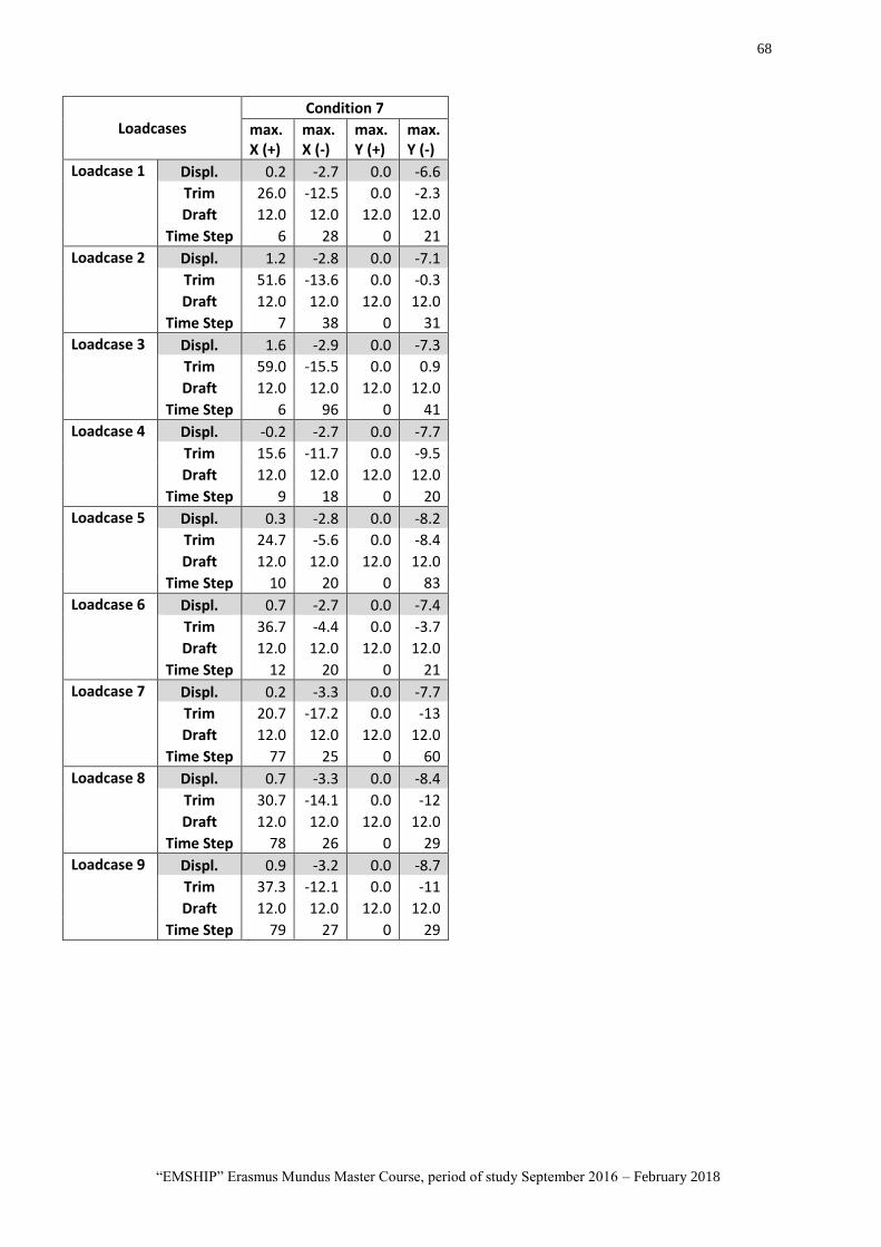
68
“EMSHIP” Erasmus Mundus Master Course, period of study September 2016 – February 2018
Loadcases Condition 7
max. X (+)
max. X (-)
max. Y (+)
max. Y (-)
Loadcase 1 Displ. 0.2 -2.7 0.0 -6.6
Trim 26.0 -12.5 0.0 -2.3
Draft 12.0 12.0 12.0 12.0
Time Step 6 28 0 21
Loadcase 2 Displ. 1.2 -2.8 0.0 -7.1
Trim 51.6 -13.6 0.0 -0.3
Draft 12.0 12.0 12.0 12.0
Time Step 7 38 0 31
Loadcase 3 Displ. 1.6 -2.9 0.0 -7.3
Trim 59.0 -15.5 0.0 0.9
Draft 12.0 12.0 12.0 12.0
Time Step 6 96 0 41
Loadcase 4 Displ. -0.2 -2.7 0.0 -7.7
Trim 15.6 -11.7 0.0 -9.5
Draft 12.0 12.0 12.0 12.0
Time Step 9 18 0 20
Loadcase 5 Displ. 0.3 -2.8 0.0 -8.2
Trim 24.7 -5.6 0.0 -8.4
Draft 12.0 12.0 12.0 12.0
Time Step 10 20 0 83
Loadcase 6 Displ. 0.7 -2.7 0.0 -7.4
Trim 36.7 -4.4 0.0 -3.7
Draft 12.0 12.0 12.0 12.0
Time Step 12 20 0 21
Loadcase 7 Displ. 0.2 -3.3 0.0 -7.7
Trim 20.7 -17.2 0.0 -13
Draft 12.0 12.0 12.0 12.0
Time Step 77 25 0 60
Loadcase 8 Displ. 0.7 -3.3 0.0 -8.4
Trim 30.7 -14.1 0.0 -12
Draft 12.0 12.0 12.0 12.0
Time Step 78 26 0 29
Loadcase 9 Displ. 0.9 -3.2 0.0 -8.7
Trim 37.3 -12.1 0.0 -11
Draft 12.0 12.0 12.0 12.0
Time Step 79 27 0 29
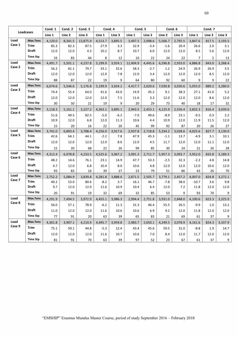
69
“EMSHIP” Erasmus Mundus Master Course, period of study September 2016 – February 2018
Loadcases Cond. 1 Cond. 2 Cond. 3 Cond. 4 Cond. 5 Cond. 6 Cond. 7
Line 1 Line 2 Line 3 Line 1 Line 3 Line 1 Line 2 Line 2 Line 3 Line 1 Line 2 Line 3
Load Case 1
Max.Tens 4,120.0 8,341.5 13,875.9 4,513.7 3,895.5 3,497.5 2,098.6 5,566.7 2,792.5 3,847.6 817.5 3,193.5
Trim 85.3 82.3 87.5 27.9 3.3 32.9 -3.4 -1.6 20.4 26.6 2.0 3.1
Draft 12.0 12.0 4.3 10.2 8.7 10.7 6.0 12.0 12.0 8.5 5.6 12.0
Time Stp 33 83 44 8 12 10 22 24 22 7 2 13
Load Case 2
Max.Tens 4,491.7 5,501.1 4,237.8 5,199.9 3,924.1 12,404.9 4,445.6 6,596.8 2,933.0 4,886.8 843.0 3,268.4
Trim 56.2 81.1 79.7 33.1 32.6 58.3 -2.7 1.2 24.9 26.9 26.9 3.5
Draft 12.0 12.0 12.0 12.0 7.8 12.0 3.4 12.0 12.0 12.0 8.5 12.0
Time Stp 88 87 22 19 9 64 80 92 60 9 9 22
Load Case 3
Max.Tens 6,074.6 5,546.6 5,176.8 5,199.9 3,924.1 4,417.7 2,620.6 7,030.8 3,030.6 5,055.0 889.2 3,280.0
Trim 74.4 55.4 64.0 41.6 43.0 14.9 45.2 9.1 38.3 27.1 41.0 5.2
Draft 12.0 12.0 12.0 12.0 7.5 11.6 3.3 12.0 12.0 12.0 8.6 12.0
Time Stp 30 50 21 19 9 20 29 73 40 18 17 32
Load Case 4
Max.Tens 3,118.3 5,161.1 3,227.2 4,363.1 3,895.1 2,943.5 2,453.1 4,125.9 2,556.4 3,832.3 816.4 3,039.0
Trim 51.6 49.5 82.5 -5.0 -6.2 -7.0 49.6 -8.9 23.1 -9.5 0.3 2.2
Draft 10.9 12.0 6.8 12.0 11.3 10.6 4.4 10.9 12.0 11.9 11.5 12.0
Time Stp 15 20 16 22 20 45 99 92 87 20 26 27
Load Case 5
Max.Tens 3,741.0 6,893.4 3,788.4 4,256.0 3,917.6 2,937.8 2,718.8 5,334.2 3,028.6 4,025.6 827.7 3,130.0
Trim 42.6 64.1 44.1 -2.2 7.8 47.9 45.3 -1.1 13.7 -4.9 3.1 10.1
Draft 12.0 12.0 12.0 12.0 8.6 12.0 4.5 11.7 12.0 12.0 11.1 12.0
Time Stp 15 20 68 22 26 99 85 30 24 21 26 28
Load Case 6
Max.Tens 4,312.4 6,978.8 4,233.5 4,525.6 3,967.2 3,091.3 2,711.7 5,957.3 3,093.7 3,952.0 833.8 3,189.3
Trim 48.2 14.6 76.1 23.1 14.9 47.7 53.3 -2.5 32.3 -2.2 4.8 14.8
Draft 4.7 12.0 6.8 10.4 8.0 10.6 4.8 12.0 12.0 12.0 10.6 12.0
Time Stp 93 83 16 39 27 23 79 51 86 43 26 70
Load Case 7
Max.Tens 2,752.2 5,084.9 3,839.8 4,281.8 3,888.6 2,871.5 2,505.7 3,779.1 2,457.2 4,007.0 824.8 3,272.1
Trim 49.2 53.0 80.6 -8.2 3.7 16.1 46.7 -7.8 38.0 -10.7 3.6 9.8
Draft 9.7 12.0 12.0 11.6 10.9 10.4 6.4 12.0 7.2 11.8 12.0 12.0
Time Stp 20 91 19 32 69 32 85 53 9 93 70 9
Load Case 8
Max.Tens 4,291.9 7,494.5 3,972.9 4,455.1 3,986.3 2,994.4 2,751.8 3,931.0 2,848.0 4,100.6 823.3 3,325.9
Trim 56.0 57.1 78.9 -6.2 11.3 31.3 46.4 55.5 26.5 -9.9 1.0 13.2
Draft 11.0 12.0 12.0 11.6 10.6 10.6 6.9 9.2 12.0 11.8 12.0 12.0
Time Stp 77 91 20 63 39 65 83 21 69 61 37 9
Load Case 9
Max.Tens 4,301.8 3,907.1 4,210.9 4,495.7 3,959.8 2,983.7 2,650.1 4,249.5 3,078.9 4,161.6 824.3 3,337.9
Trim 75.1 59.1 44.8 -5.3 12.4 43.4 45.6 59.5 31.0 -8.8 1.9 14.7
Draft 12.0 12.0 12.0 11.6 10.7 10.6 7.0 8.4 12.0 11.7 12.0 12.0
Time Stp 81 91 70 63 39 97 52 23 67 61 37 9
70
“EMSHIP” Erasmus Mundus Master Course, period of study September 2016 – February 2018
APPENDIXES B. MATLAB CODES OF MORISON
HYDRODYNAMIC LOAD ALGORITHM FOR CYLINDER
FLOATING STRUCTURE
ABREVIATIATIONS
xyzKar = xyz-Kardan angles
T = Transformation Matrix
N = amount of time variant
rMaLoc = positions of markers on body
ampli = amplitude
rRef = Position of body Ref. Global sys.
vRef = Velocity of the body
Ut4D = wave velocity at XYZ global axis
omRef = Angular velocity of the body
dUt4D = wave acceleration at XYZ global axis
nMarkers = Number of markers
u_rel4D = relative velocity at XYZ global axis
r_CSYS_0 = Global Positions of markers
dUt_totx2D = final acc. wrto wave elev at X local axis
v_CSYS_0 = Global velocity of markers
u_totx2D = final vel. wrto wave elev at X local axis
k = wave elevation
u_totz2D = final vel. wrto wave elev at Z local axis
z_eta2D = Marker points in z axis wrto Wave elevation
eta2D = wave elevation for each marker point
Id = Identity to filter all results wrto wave elevation
Re_U = Reynold Number to obtain added mass and drag coefficient in
horizontal dir.
Kc_U = Keulegan Number to obtain added mass and drag coefficient in
horizontal dir.
Cm_U = Added Mass Coefficient
Cd_U = Drag Coefficient
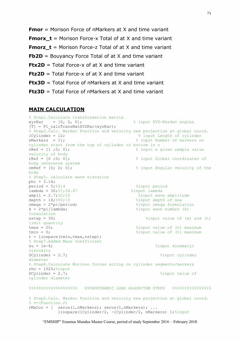
71
“EMSHIP” Erasmus Mundus Master Course, period of study September 2016 – February 2018
Fmor = Morison Force of nMarkers at X and time variant
Fmorx_t = Morison Force-x Total of at X and time variant
Fmorz_t = Morison Force-z Total of at X and time variant
Fb2D = Bouyancy Force Total of at X and time variant
Ftx2D = Total Force-x of at X and time variant
Ftz2D = Total Force-x of at X and time variant
Ftx3D = Total Force of nMarkers at X and time variant
Ftz3D = Total Force of nMarkers at X and time variant
MAIN CALCULATION
% Step1.Calculate transformation matrix xyzKar = [0, 0, 0]; % input XYZ-Kardan angles [T] = F1_calcTransMatXYZKar(xyzKar); % Step2.Calc. Marker Position and velocity new projection at global coord. lCylinder = 12; % input Length of cylinder nMarkers = 11; % input Number of markers on
cylinder start from the top of cylinder to bottom in z vRef = [1 ;0; 0]; % input a given sample value
velocity of body rRef = [0 ;0; 0]; % input Global coordinates of
body reference system omRef = [0; 0; 0]; % input Angular velocity of the
body % Step3. calculate wave elevation phi = 3.14; period = 5;%2;4 %input period lambda = 30;%1;24.67 %input lambda ampli = 2.7;%2;10 %input wave amplitude depth = 16;%50;10 %input depth of sea omega = 2*pi/period; %input omega formulation k = 2*pi/lambda; %input wave number (k)
formulation nstep = 30; %input value of (x) and (t)
limit quantity tmax = 25; %input value of (t) maximum tmin = 0; %input value of (t) maximum t = linspace(tmin,tmax,nstep); % Step7.Added Mass Coefficient nu = 1e-6; %input kinematic
viscosity DCylinder = 2.7; %input cylinder
diameter % Step8.Calculate Morison forces acting on cylinder segments/markers rho = 1025;%input DCylinder = 2.7; %input value of
cylinder diameter
%%%%%%%%%%%%%%%%%%%% HYDRODYNAMIC LOAD ALGORITHM STEPS %%%%%%%%%%%%%%%%
% Step2.Calc. Marker Position and velocity new projection at global coord. % ==(Function.2) rMaLoc = [ zeros(1,nMarkers); zeros(1,nMarkers); ... linspace(lCylinder/2, -lCylinder/2, nMarkers) ];%input
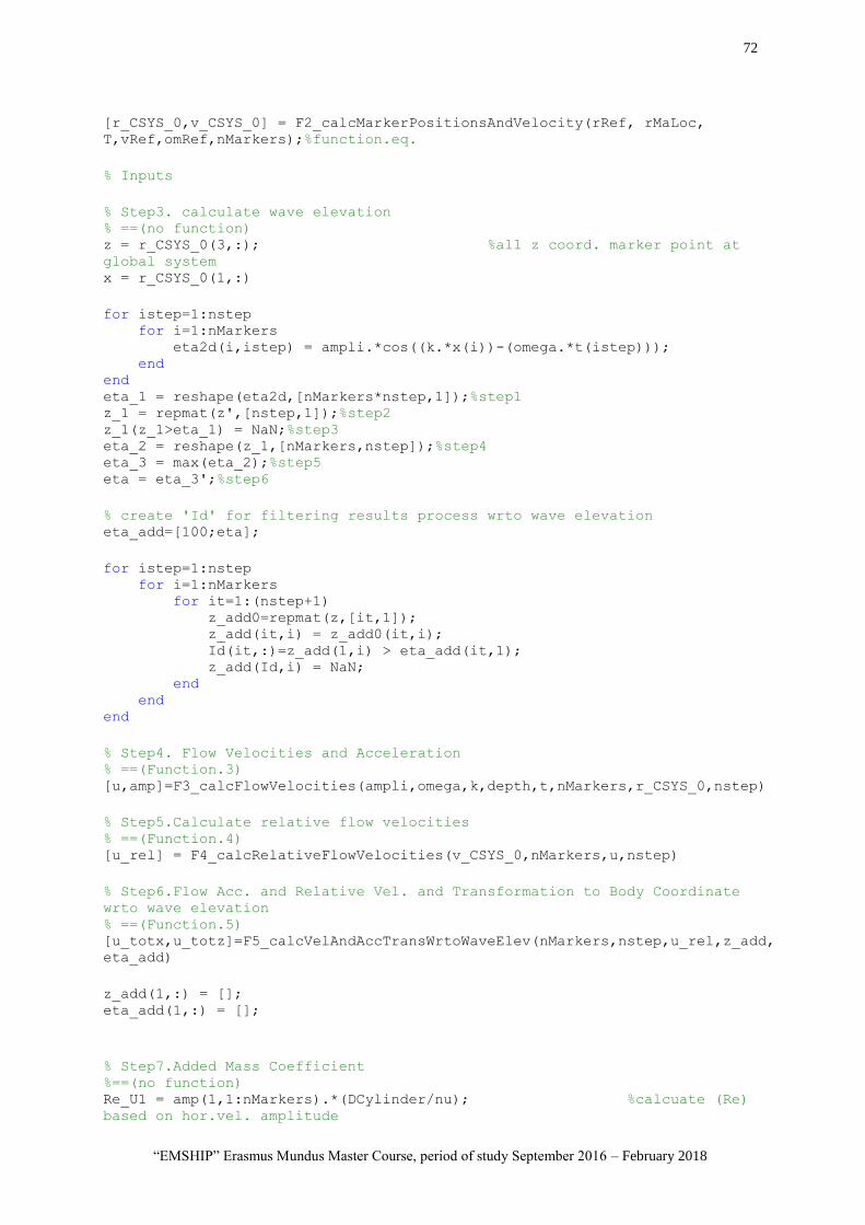
72
“EMSHIP” Erasmus Mundus Master Course, period of study September 2016 – February 2018
[r_CSYS_0,v_CSYS_0] = F2_calcMarkerPositionsAndVelocity(rRef, rMaLoc,
T,vRef,omRef,nMarkers);%function.eq.
% Inputs
% Step3. calculate wave elevation % ==(no function) z = r_CSYS_0(3,:); %all z coord. marker point at
global system x = r_CSYS_0(1,:)
for istep=1:nstep for i=1:nMarkers eta2d(i,istep) = ampli.*cos((k.*x(i))-(omega.*t(istep))); end end eta_1 = reshape(eta2d,[nMarkers*nstep,1]);%step1 z_1 = repmat(z',[nstep,1]);%step2 z_1(z_1>eta_1) = NaN;%step3 eta_2 = reshape(z_1,[nMarkers,nstep]);%step4 eta_3 = max(eta_2);%step5 eta = eta_3';%step6
% create 'Id' for filtering results process wrto wave elevation eta_add=[100;eta];
for istep=1:nstep for i=1:nMarkers for it=1:(nstep+1) z_add0=repmat(z,[it,1]); z_add(it,i) = z_add0(it,i); Id(it,:)=z_add(1,i) > eta_add(it,1); z_add(Id,i) = NaN; end end end
% Step4. Flow Velocities and Acceleration % ==(Function.3) [u,amp]=F3_calcFlowVelocities(ampli,omega,k,depth,t,nMarkers,r_CSYS_0,nstep)
% Step5.Calculate relative flow velocities % ==(Function.4) [u_rel] = F4_calcRelativeFlowVelocities(v_CSYS_0,nMarkers,u,nstep)
% Step6.Flow Acc. and Relative Vel. and Transformation to Body Coordinate
wrto wave elevation % ==(Function.5) [u_totx,u_totz]=F5_calcVelAndAccTransWrtoWaveElev(nMarkers,nstep,u_rel,z_add,
eta_add)
z_add(1,:) = []; eta_add(1,:) = [];
% Step7.Added Mass Coefficient %==(no function) Re_U1 = amp(1,1:nMarkers).*(DCylinder/nu); %calcuate (Re)
based on hor.vel. amplitude
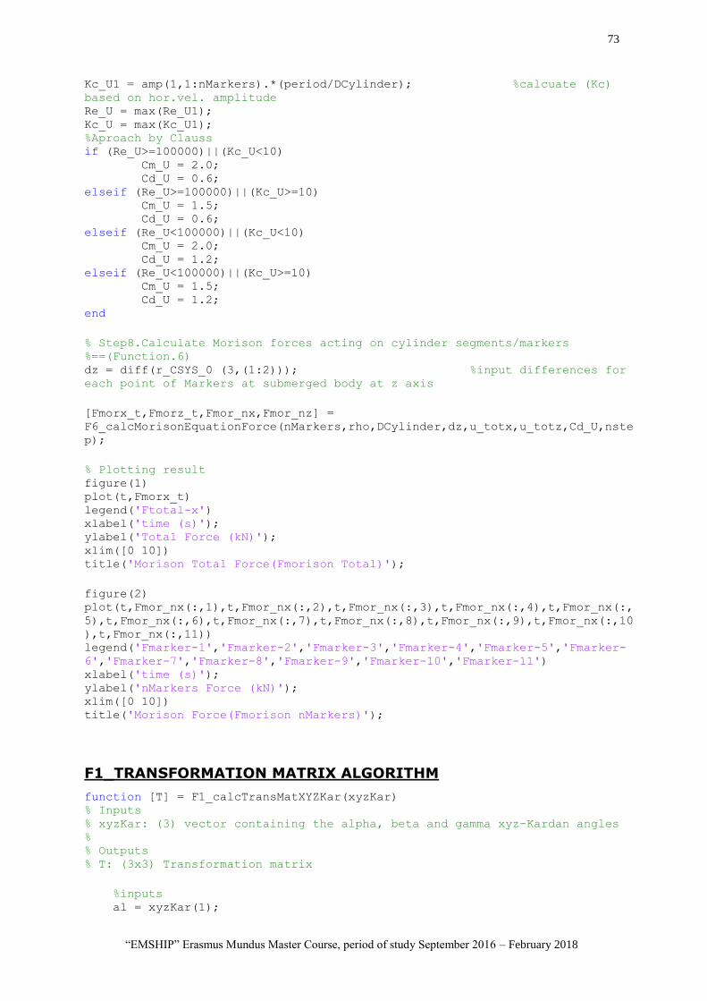
73
“EMSHIP” Erasmus Mundus Master Course, period of study September 2016 – February 2018
Kc_U1 = amp(1,1:nMarkers).*(period/DCylinder); %calcuate (Kc)
based on hor.vel. amplitude Re_U = max(Re_U1); Kc_U = max(Kc_U1); %Aproach by Clauss if (Re_U>=100000)||(Kc_U<10) Cm_U = 2.0; Cd_U = 0.6; elseif (Re_U>=100000)||(Kc_U>=10) Cm_U = 1.5; Cd_U = 0.6; elseif (Re_U<100000)||(Kc_U<10) Cm_U = 2.0; Cd_U = 1.2; elseif (Re_U<100000)||(Kc_U>=10) Cm_U = 1.5; Cd_U = 1.2; end
% Step8.Calculate Morison forces acting on cylinder segments/markers %==(Function.6) dz = diff(r_CSYS_0 (3,(1:2))); %input differences for
each point of Markers at submerged body at z axis
[Fmorx_t,Fmorz_t,Fmor_nx,Fmor_nz] =
F6_calcMorisonEquationForce(nMarkers,rho,DCylinder,dz,u_totx,u_totz,Cd_U,nste
p);
% Plotting result figure(1) plot(t,Fmorx_t) legend('Ftotal-x') xlabel('time (s)'); ylabel('Total Force (kN)'); xlim([0 10]) title('Morison Total Force(Fmorison Total)');
figure(2) plot(t,Fmor_nx(:,1),t,Fmor_nx(:,2),t,Fmor_nx(:,3),t,Fmor_nx(:,4),t,Fmor_nx(:,
5),t,Fmor_nx(:,6),t,Fmor_nx(:,7),t,Fmor_nx(:,8),t,Fmor_nx(:,9),t,Fmor_nx(:,10
),t,Fmor_nx(:,11)) legend('Fmarker-1','Fmarker-2','Fmarker-3','Fmarker-4','Fmarker-5','Fmarker-
6','Fmarker-7','Fmarker-8','Fmarker-9','Fmarker-10','Fmarker-11') xlabel('time (s)'); ylabel('nMarkers Force (kN)'); xlim([0 10]) title('Morison Force(Fmorison nMarkers)');
F1_TRANSFORMATION MATRIX ALGORITHM
function [T] = F1_calcTransMatXYZKar(xyzKar) % Inputs % xyzKar: (3) vector containing the alpha, beta and gamma xyz-Kardan angles % % Outputs % T: (3x3) Transformation matrix
%inputs al = xyzKar(1);
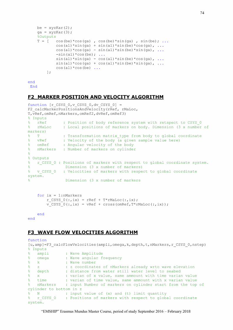
74
“EMSHIP” Erasmus Mundus Master Course, period of study September 2016 – February 2018
be = xyzKar(2); ga = xyzKar(3); %Outputs T = [ cos(be)*cos(ga) , cos(be)*sin(ga) , sin(be); ... cos(al)*sin(ga) + sin(al)*sin(be)*cos(ga), ... cos(al)*cos(ga) - sin(al)*sin(be)*sin(ga), ... -sin(al)*cos(be); ... sin(al)*sin(ga) - cos(al)*sin(be)*cos(ga), ... sin(al)*cos(ga) + cos(al)*sin(be)*sin(ga), ... cos(al)*cos(be) ... ];
end End
F2_MARKER POSITION AND VELOCITY ALGORITHM
function [r_CSYS_0,v_CSYS_0,dv_CSYS_0] =
F2_calcMarkerPositionsAndVelocity(rRef, rMaLoc,
T,vRef,omRef,nMarkers,omRef2,dvRef,omRef3) % Inputs % rRef : Position of body reference system with retspect to CSYS_0 % rMaLoc : Local positions of markers on body. Dimension (3 x number of
markers) % T : Transformation matrix_type from body to global coordinate % vRef : Velocity of the body (a given sample value here) % omRef : Angular velocity of the body % nMarkers : Number of markers on cylinder % % Outputs % r_CSYS_0 : Positions of markers with respect to global coordinate system. % Dimension (3 x number of markers) % v_CSYS_0 : Velocities of markers with respect to global coordinate
system. % Dimension (3 x number of markers
for ix = 1:nMarkers r_CSYS_0(:,ix) = rRef + T*rMaLoc(:,ix); v_CSYS_0(:,ix) = vRef + cross(omRef,T*rMaLoc(:,ix));
end end
F3_WAVE FLOW VELOCITIES ALGORITHM
function
[u,amp]=F3_calcFlowVelocities(ampli,omega,k,depth,t,nMarkers,r_CSYS_0,nstep) % Inputs % ampli : Wave Amplitude % omega : Wave angular frequency % k : Wave number % z : z coordinates of nMarkers already wrto wave elevation % depth : distance from water still water level to seabed % x : varian of x value, same ammount with time varian value % time : varian of time value, same ammount with x varian value % nMarkers : input Number of markers on cylinder start from the top of
cylinder to bottom in z % N : input value of (x) and (t) limit quantity % r_CSYS_0 : Positions of markers with respect to global coordinate
system.
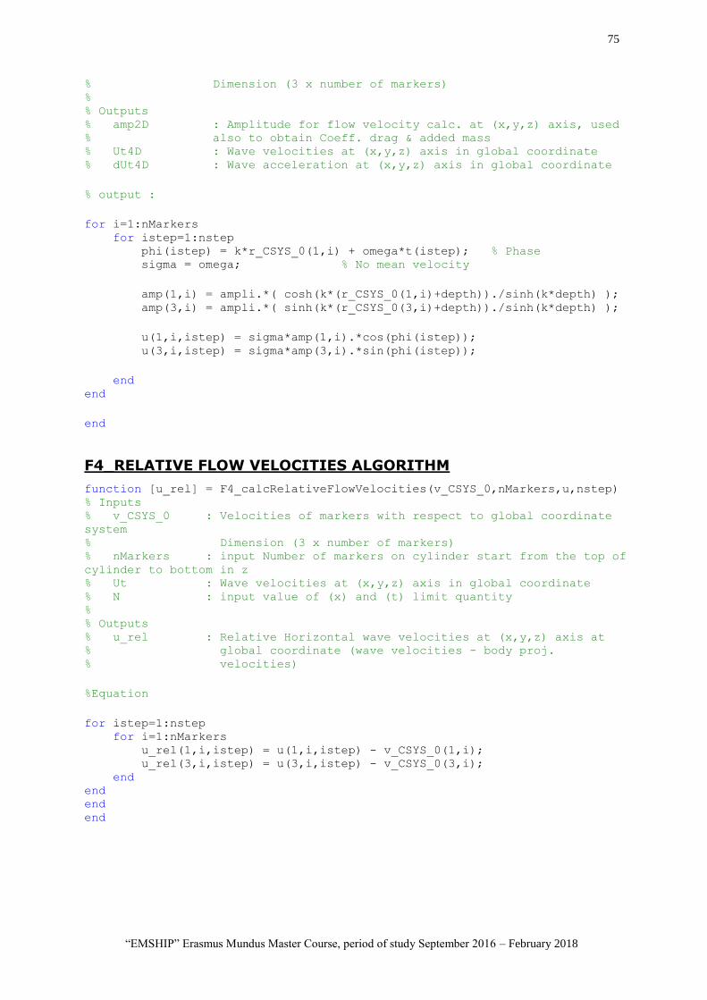
75
“EMSHIP” Erasmus Mundus Master Course, period of study September 2016 – February 2018
% Dimension (3 x number of markers) % % Outputs % amp2D : Amplitude for flow velocity calc. at (x,y,z) axis, used % also to obtain Coeff. drag & added mass % Ut4D : Wave velocities at (x,y,z) axis in global coordinate % dUt4D : Wave acceleration at (x,y,z) axis in global coordinate
% output :
for i=1:nMarkers for istep=1:nstep phi(istep) = k*r_CSYS_0(1,i) + omega*t(istep); % Phase sigma = omega; % No mean velocity
amp(1,i) = ampli.*( cosh(k*(r_CSYS_0(1,i)+depth))./sinh(k*depth) ); amp(3,i) = ampli.*( sinh(k*(r_CSYS_0(3,i)+depth))./sinh(k*depth) );
u(1,i,istep) = sigma*amp(1,i).*cos(phi(istep)); u(3,i,istep) = sigma*amp(3,i).*sin(phi(istep));
end end
end
F4_RELATIVE FLOW VELOCITIES ALGORITHM
function [u_rel] = F4_calcRelativeFlowVelocities(v_CSYS_0,nMarkers,u,nstep) % Inputs % v_CSYS_0 : Velocities of markers with respect to global coordinate
system % Dimension (3 x number of markers) % nMarkers : input Number of markers on cylinder start from the top of
cylinder to bottom in z % Ut : Wave velocities at (x,y,z) axis in global coordinate % N : input value of (x) and (t) limit quantity % % Outputs % u_rel : Relative Horizontal wave velocities at (x,y,z) axis at % global coordinate (wave velocities - body proj. % velocities)
%Equation
for istep=1:nstep for i=1:nMarkers u_rel(1,i,istep) = u(1,i,istep) - v_CSYS_0(1,i); u_rel(3,i,istep) = u(3,i,istep) - v_CSYS_0(3,i); end end end end
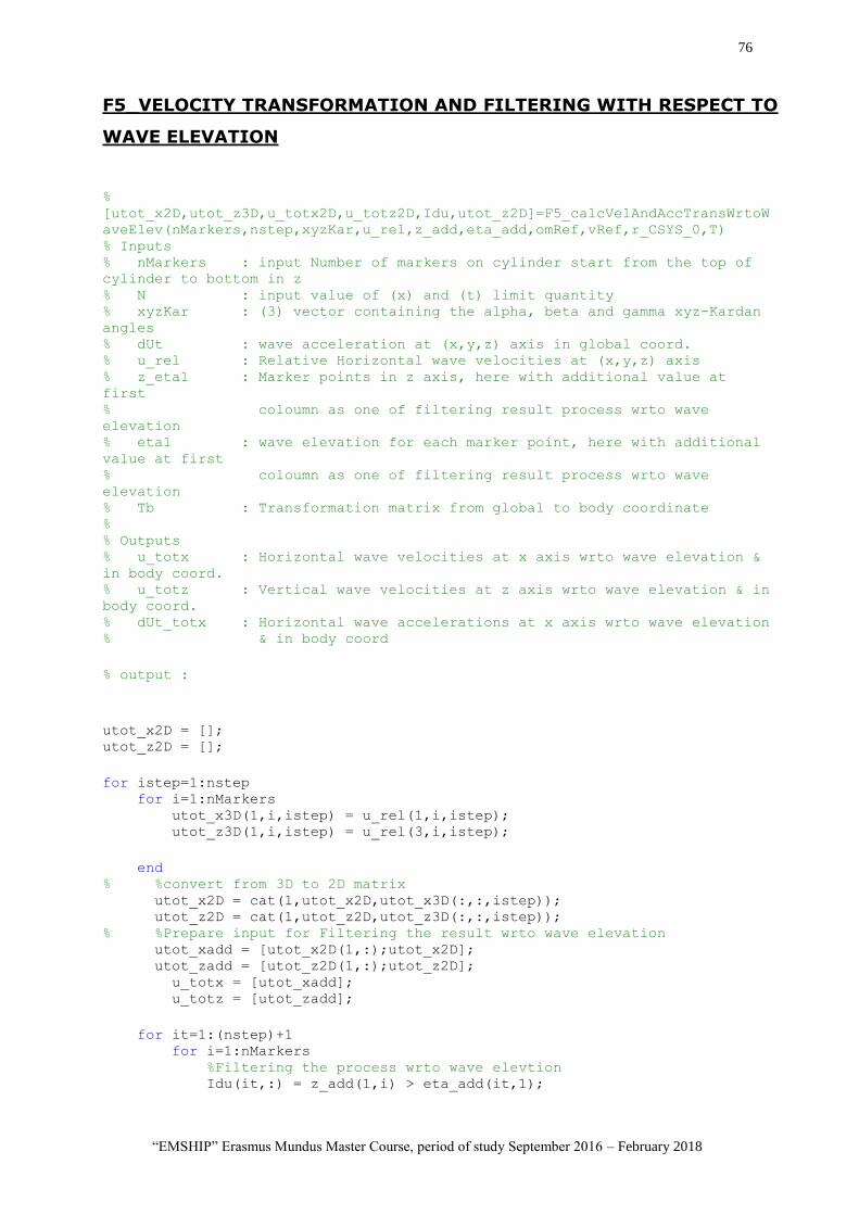
76
“EMSHIP” Erasmus Mundus Master Course, period of study September 2016 – February 2018
F5_VELOCITY TRANSFORMATION AND FILTERING WITH RESPECT TO
WAVE ELEVATION
%
[utot_x2D,utot_z3D,u_totx2D,u_totz2D,Idu,utot_z2D]=F5_calcVelAndAccTransWrtoW
aveElev(nMarkers,nstep,xyzKar,u_rel,z_add,eta_add,omRef,vRef,r_CSYS_0,T) % Inputs % nMarkers : input Number of markers on cylinder start from the top of
cylinder to bottom in z % N : input value of (x) and (t) limit quantity % xyzKar : (3) vector containing the alpha, beta and gamma xyz-Kardan
angles % dUt : wave acceleration at (x,y,z) axis in global coord. % u_rel : Relative Horizontal wave velocities at (x,y,z) axis % z_eta1 : Marker points in z axis, here with additional value at
first % coloumn as one of filtering result process wrto wave
elevation % eta1 : wave elevation for each marker point, here with additional
value at first % coloumn as one of filtering result process wrto wave
elevation % Tb : Transformation matrix from global to body coordinate % % Outputs % u_totx : Horizontal wave velocities at x axis wrto wave elevation &
in body coord. % u_totz : Vertical wave velocities at z axis wrto wave elevation & in
body coord. % dUt_totx : Horizontal wave accelerations at x axis wrto wave elevation % & in body coord
% output :
utot_x2D = []; utot_z2D = [];
for istep=1:nstep for i=1:nMarkers utot_x3D(1,i,istep) = u_rel(1,i,istep); utot_z3D(1,i,istep) = u_rel(3,i,istep);
end % %convert from 3D to 2D matrix utot_x2D = cat(1,utot_x2D,utot_x3D(:,:,istep)); utot_z2D = cat(1,utot_z2D,utot_z3D(:,:,istep)); % %Prepare input for Filtering the result wrto wave elevation utot_xadd = [utot_x2D(1,:);utot_x2D]; utot_zadd = [utot_z2D(1,:);utot_z2D]; u_totx = [utot_xadd]; u_totz = [utot_zadd];
for it=1:(nstep)+1 for i=1:nMarkers %Filtering the process wrto wave elevtion Idu(it,:) = z_add(1,i) > eta_add(it,1);
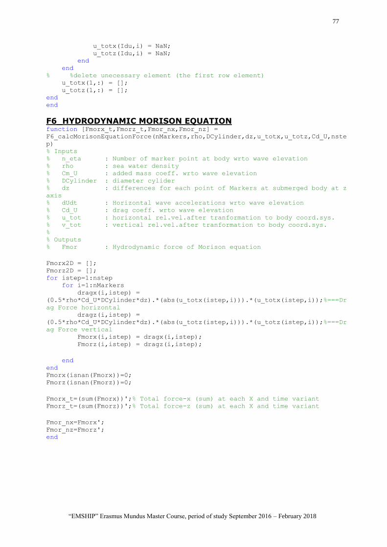
77
“EMSHIP” Erasmus Mundus Master Course, period of study September 2016 – February 2018
u_totx(Idu,i) = NaN; u_totz(Idu,i) = NaN; end end % %delete unecessary element (the first row element) u_totx(1,:) = []; u_totz(1,:) = []; end end
F6_HYDRODYNAMIC MORISON EQUATION function [Fmorx_t,Fmorz_t,Fmor_nx,Fmor_nz] =
F6_calcMorisonEquationForce(nMarkers,rho,DCylinder,dz,u_totx,u_totz,Cd_U,nste
p) % Inputs % n_eta : Number of marker point at body wrto wave elevation % rho : sea water density % Cm_U : added mass coeff. wrto wave elevation % DCylinder : diameter cylider % dz : differences for each point of Markers at submerged body at z
axis % dUdt : Horizontal wave accelerations wrto wave elevation % Cd_U : drag coeff. wrto wave elevation % u_tot : horizontal rel.vel.after tranformation to body coord.sys. % v_tot : vertical rel.vel.after tranformation to body coord.sys. % % Outputs % Fmor : Hydrodynamic force of Morison equation
Fmorx2D = []; Fmorz2D = []; for istep=1:nstep for i=1:nMarkers dragx(i,istep) =
(0.5*rho*Cd_U*DCylinder*dz).*(abs(u_totx(istep,i))).*(u_totx(istep,i));%===Dr
ag Force horizontal dragz(i,istep) =
(0.5*rho*Cd_U*DCylinder*dz).*(abs(u_totz(istep,i))).*(u_totz(istep,i));%===Dr
ag Force vertical Fmorx(i,istep) = dragx(i,istep); Fmorz(i,istep) = dragz(i,istep);
end end Fmorx(isnan(Fmorx))=0; Fmorz(isnan(Fmorz))=0;
Fmorx_t=(sum(Fmorx))';% Total force-x (sum) at each X and time variant Fmorz_t=(sum(Fmorz))';% Total force-z (sum) at each X and time variant
Fmor_nx=Fmorx'; Fmor_nz=Fmorz'; end
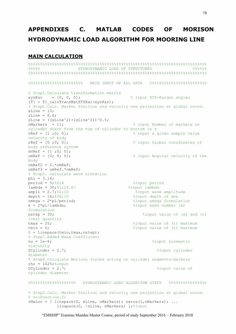
78
“EMSHIP” Erasmus Mundus Master Course, period of study September 2016 – February 2018
APPENDIXES C. MATLAB CODES OF MORISON
HYDRODYNAMIC LOAD ALGORITHM FOR MOORING LINE
MAIN CALCULATION
%%%%%%%%%%%%%%%%%%%%%%%%%%%%%%%%%%%%%%%%%%%%%%%%%%%%%%%%%%%%%%%%%%%%%%%%%%% %%%%% HYDRODYNAMIC LOAD OF STRUCTURES %%%%%% %%%%%%%%%%%%%%%%%%%%%%%%%%%%%%%%%%%%%%%%%%%%%%%%%%%%%%%%%%%%%%%%%%%%%%%%%%%
%%%%%%%%%%%%%%%%%%%%%%% MAIN INPUT OF ALL DATA %%%%%%%%%%%%%%%%%%%%%%%%
% Step1.Calculate transformation matrix xyzKar = [0, 0, 0]; % input XYZ-Kardan angles [T] = F1_calcTransMatXYZKar(xyzKar); % Step2.Calc. Marker Position and velocity new projection at global coord. xLine = 10; zLine = 6.6; sLine = ((xLine^2)+(zLine^2))^0.5; nMarkers = 11; % input Number of markers on
cylinder start from the top of cylinder to bottom in z vRef = [1 ;0; 0]; % input a given sample value
velocity of body rRef = [0 ;0; 0]; % input Global coordinates of
body reference system dvRef = [1 ;0; 0]; omRef = [0; 0; 0]; % input Angular velocity of the
body omRef2 = 2.*omRef; omRef3 = omRef.*omRef; % Step3. calculate wave elevation phi = 3.14; period = 5;%2;4 %input period lambda = 30;%1;24.67 %input lambda ampli = 2.7;%2;10 %input wave amplitude depth = 16;%50;10 %input depth of sea omega = 2*pi/period; %input omega formulation k = 2*pi/lambda; %input wave number (k)
formulation nstep = 30; %input value of (x) and (t)
limit quantity tmax = 25; %input value of (t) maximum tmin = 0; %input value of (t) maximum t = linspace(tmin,tmax,nstep); % Step7.Added Mass Coefficient nu = 1e-6; %input kinematic
viscosity DCylinder = 2.7; %input cylinder
diameter % Step8.Calculate Morison forces acting on cylinder segments/markers rho = 1025;%input DCylinder = 2.7; %input value of
cylinder diameter
%%%%%%%%%%%%%%%%%%%% HYDRODYNAMIC LOAD ALGORITHM STEPS %%%%%%%%%%%%%%%%
% Step2.Calc. Marker Position and velocity new projection at global coord. % ==(Function.2) rMaLoc = [ linspace(0, xLine, nMarkers); zeros(1,nMarkers); ... linspace(0, -zLine, nMarkers) ];%input
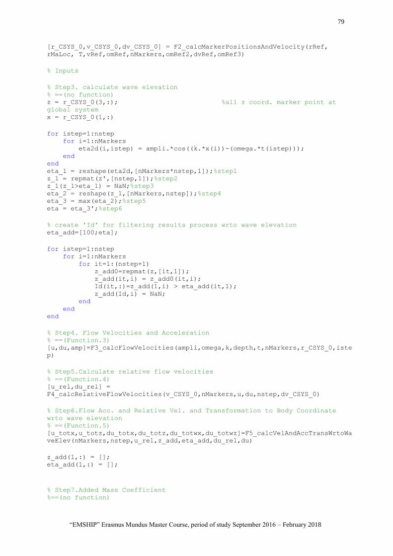
79
“EMSHIP” Erasmus Mundus Master Course, period of study September 2016 – February 2018
[r_CSYS_0,v_CSYS_0,dv_CSYS_0] = F2_calcMarkerPositionsAndVelocity(rRef,
rMaLoc, T,vRef,omRef,nMarkers,omRef2,dvRef,omRef3)
% Inputs
% Step3. calculate wave elevation % ==(no function) z = r_CSYS_0(3,:); %all z coord. marker point at
global system x = r_CSYS_0(1,:)
for istep=1:nstep for i=1:nMarkers eta2d(i,istep) = ampli.*cos((k.*x(i))-(omega.*t(istep))); end end eta_1 = reshape(eta2d,[nMarkers*nstep,1]);%step1 z_1 = repmat(z',[nstep,1]);%step2 z_1(z_1>eta_1) = NaN;%step3 eta_2 = reshape(z_1,[nMarkers,nstep]);%step4 eta_3 = max(eta_2);%step5 eta = eta_3';%step6
% create 'Id' for filtering results process wrto wave elevation eta_add=[100;eta];
for istep=1:nstep for i=1:nMarkers for it=1:(nstep+1) z_add0=repmat(z,[it,1]); z_add(it,i) = z_add0(it,i); Id(it,:)=z_add(1,i) > eta_add(it,1); z_add(Id,i) = NaN; end end end
% Step4. Flow Velocities and Acceleration % ==(Function.3) [u,du,amp]=F3_calcFlowVelocities(ampli,omega,k,depth,t,nMarkers,r_CSYS_0,iste
p)
% Step5.Calculate relative flow velocities % ==(Function.4) [u_rel,du_rel] =
F4_calcRelativeFlowVelocities(v_CSYS_0,nMarkers,u,du,nstep,dv_CSYS_0)
% Step6.Flow Acc. and Relative Vel. and Transformation to Body Coordinate
wrto wave elevation % ==(Function.5) [u_totx,u_totz,du_totx,du_totz,du_totwx,du_totwz]=F5_calcVelAndAccTransWrtoWa
veElev(nMarkers,nstep,u_rel,z_add,eta_add,du_rel,du)
z_add(1,:) = []; eta_add(1,:) = [];
% Step7.Added Mass Coefficient %==(no function)
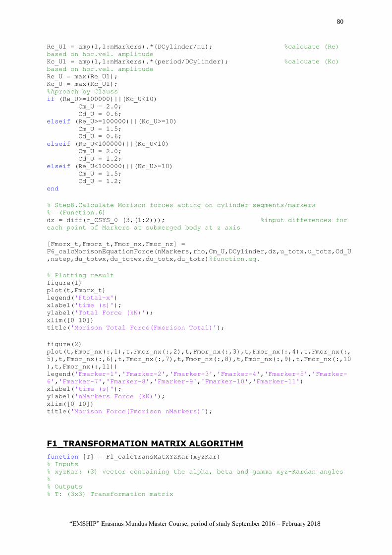
80
“EMSHIP” Erasmus Mundus Master Course, period of study September 2016 – February 2018
Re_U1 = amp(1,1:nMarkers).*(DCylinder/nu); %calcuate (Re)
based on hor.vel. amplitude Kc_U1 = amp(1,1:nMarkers).*(period/DCylinder); %calcuate (Kc)
based on hor.vel. amplitude Re_U = max(Re_U1); Kc_U = max(Kc_U1); %Aproach by Clauss if (Re_U>=100000)||(Kc_U<10) Cm_U = 2.0; Cd_U = 0.6; elseif (Re_U>=100000)||(Kc_U>=10) Cm_U = 1.5; Cd_U = 0.6; elseif (Re_U<100000)||(Kc_U<10) Cm_U = 2.0; Cd_U = 1.2; elseif (Re_U<100000)||(Kc_U>=10) Cm_U = 1.5; Cd_U = 1.2; end
% Step8.Calculate Morison forces acting on cylinder segments/markers %==(Function.6) dz = diff(r_CSYS_0 (3,(1:2))); %input differences for
each point of Markers at submerged body at z axis
[Fmorx_t,Fmorz_t,Fmor_nx,Fmor_nz] =
F6_calcMorisonEquationForce(nMarkers,rho,Cm_U,DCylinder,dz,u_totx,u_totz,Cd_U
,nstep,du_totwx,du_totwz,du_totx,du_totz)%function.eq.
% Plotting result figure(1) plot(t,Fmorx_t) legend('Ftotal-x') xlabel('time (s)'); ylabel('Total Force (kN)'); xlim([0 10]) title('Morison Total Force(Fmorison Total)');
figure(2) plot(t,Fmor_nx(:,1),t,Fmor_nx(:,2),t,Fmor_nx(:,3),t,Fmor_nx(:,4),t,Fmor_nx(:,
5),t,Fmor_nx(:,6),t,Fmor_nx(:,7),t,Fmor_nx(:,8),t,Fmor_nx(:,9),t,Fmor_nx(:,10
),t,Fmor_nx(:,11)) legend('Fmarker-1','Fmarker-2','Fmarker-3','Fmarker-4','Fmarker-5','Fmarker-
6','Fmarker-7','Fmarker-8','Fmarker-9','Fmarker-10','Fmarker-11') xlabel('time (s)'); ylabel('nMarkers Force (kN)'); xlim([0 10]) title('Morison Force(Fmorison nMarkers)');
F1_TRANSFORMATION MATRIX ALGORITHM
function [T] = F1_calcTransMatXYZKar(xyzKar) % Inputs % xyzKar: (3) vector containing the alpha, beta and gamma xyz-Kardan angles % % Outputs % T: (3x3) Transformation matrix
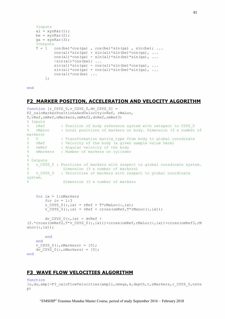
81
“EMSHIP” Erasmus Mundus Master Course, period of study September 2016 – February 2018
%inputs al = xyzKar(1); be = xyzKar(2); ga = xyzKar(3); %Outputs T = [ cos(be)*cos(ga) , cos(be)*sin(ga) , sin(be); ... cos(al)*sin(ga) + sin(al)*sin(be)*cos(ga), ... cos(al)*cos(ga) - sin(al)*sin(be)*sin(ga), ... -sin(al)*cos(be); ... sin(al)*sin(ga) - cos(al)*sin(be)*cos(ga), ... sin(al)*cos(ga) + cos(al)*sin(be)*sin(ga), ... cos(al)*cos(be) ... ];
end
F2_MARKER POSITION, ACCELERATION AND VELOCITY ALGORITHM
function [r_CSYS_0,v_CSYS_0,dv_CSYS_0] =
F2_calcMarkerPositionsAndVelocity(rRef, rMaLoc,
T,vRef,omRef,nMarkers,omRef2,dvRef,omRef3) % Inputs % rRef : Position of body reference system with retspect to CSYS_0 % rMaLoc : Local positions of markers on body. Dimension (3 x number of
markers) % T : Transformation matrix_type from body to global coordinate % vRef : Velocity of the body (a given sample value here) % omRef : Angular velocity of the body % nMarkers : Number of markers on cylinder % % Outputs % r_CSYS_0 : Positions of markers with respect to global coordinate system. % Dimension (3 x number of markers) % v_CSYS_0 : Velocities of markers with respect to global coordinate
system. % Dimension (3 x number of markers
for ix = 1:nMarkers for iv = 1:3 r_CSYS_0(:,ix) = rRef + T*rMaLoc(:,ix); v_CSYS_0(:,ix) = vRef + cross(omRef,T*rMaLoc(:,ix));
dv_CSYS_0(:,ix) = dvRef +
(2.*cross(omRef2,T*v_CSYS_0(:,ix)))+cross(omRef,rMaLoc(:,ix))+cross(omRef3,rM
aLoc(:,ix));
end end v_CSYS_0(:,nMarkers) = [0]; dv_CSYS_0(:,nMarkers) = [0]; end
F3_WAVE FLOW VELOCITIES ALGORITHM
function
[u,du,amp]=F3_calcFlowVelocities(ampli,omega,k,depth,t,nMarkers,r_CSYS_0,nste
p)
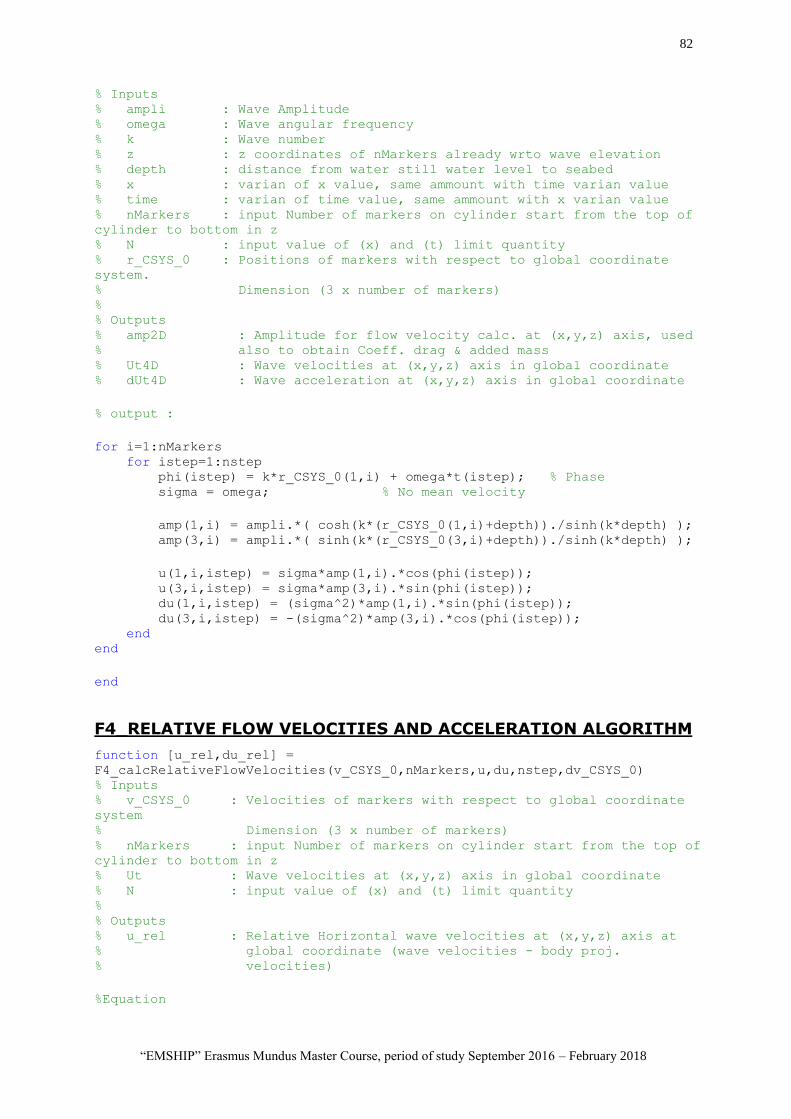
82
“EMSHIP” Erasmus Mundus Master Course, period of study September 2016 – February 2018
% Inputs % ampli : Wave Amplitude % omega : Wave angular frequency % k : Wave number % z : z coordinates of nMarkers already wrto wave elevation % depth : distance from water still water level to seabed % x : varian of x value, same ammount with time varian value % time : varian of time value, same ammount with x varian value % nMarkers : input Number of markers on cylinder start from the top of
cylinder to bottom in z % N : input value of (x) and (t) limit quantity % r_CSYS_0 : Positions of markers with respect to global coordinate
system. % Dimension (3 x number of markers) % % Outputs % amp2D : Amplitude for flow velocity calc. at (x,y,z) axis, used % also to obtain Coeff. drag & added mass % Ut4D : Wave velocities at (x,y,z) axis in global coordinate % dUt4D : Wave acceleration at (x,y,z) axis in global coordinate
% output :
for i=1:nMarkers for istep=1:nstep phi(istep) = k*r_CSYS_0(1,i) + omega*t(istep); % Phase sigma = omega; % No mean velocity
amp(1,i) = ampli.*( cosh(k*(r_CSYS_0(1,i)+depth))./sinh(k*depth) ); amp(3,i) = ampli.*( sinh(k*(r_CSYS_0(3,i)+depth))./sinh(k*depth) );
u(1,i,istep) = sigma*amp(1,i).*cos(phi(istep)); u(3,i,istep) = sigma*amp(3,i).*sin(phi(istep)); du(1,i,istep) = (sigma^2)*amp(1,i).*sin(phi(istep)); du(3,i,istep) = -(sigma^2)*amp(3,i).*cos(phi(istep)); end end
end
F4_RELATIVE FLOW VELOCITIES AND ACCELERATION ALGORITHM
function [u_rel,du_rel] =
F4_calcRelativeFlowVelocities(v_CSYS_0,nMarkers,u,du,nstep,dv_CSYS_0) % Inputs % v_CSYS_0 : Velocities of markers with respect to global coordinate
system % Dimension (3 x number of markers) % nMarkers : input Number of markers on cylinder start from the top of
cylinder to bottom in z % Ut : Wave velocities at (x,y,z) axis in global coordinate % N : input value of (x) and (t) limit quantity % % Outputs % u_rel : Relative Horizontal wave velocities at (x,y,z) axis at % global coordinate (wave velocities - body proj. % velocities)
%Equation
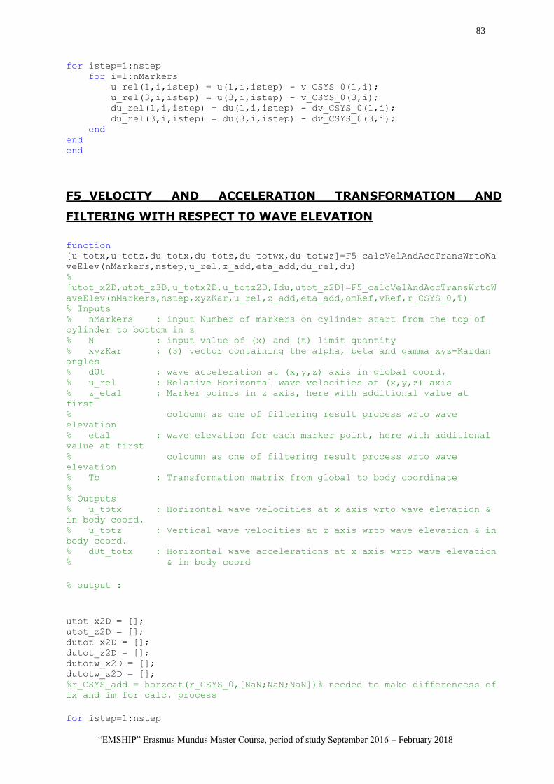
83
“EMSHIP” Erasmus Mundus Master Course, period of study September 2016 – February 2018
for istep=1:nstep for i=1:nMarkers u_rel(1,i,istep) = u(1,i,istep) - v_CSYS_0(1,i); u_rel(3,i,istep) = u(3,i,istep) - v_CSYS_0(3,i); du_rel(1,i,istep) = du(1,i,istep) - dv_CSYS_0(1,i); du_rel(3,i,istep) = du(3,i,istep) - dv_CSYS_0(3,i); end end end
F5_VELOCITY AND ACCELERATION TRANSFORMATION AND
FILTERING WITH RESPECT TO WAVE ELEVATION
function
[u_totx,u_totz,du_totx,du_totz,du_totwx,du_totwz]=F5_calcVelAndAccTransWrtoWa
veElev(nMarkers,nstep,u_rel,z_add,eta_add,du_rel,du) %
[utot_x2D,utot_z3D,u_totx2D,u_totz2D,Idu,utot_z2D]=F5_calcVelAndAccTransWrtoW
aveElev(nMarkers,nstep,xyzKar,u_rel,z_add,eta_add,omRef,vRef,r_CSYS_0,T) % Inputs % nMarkers : input Number of markers on cylinder start from the top of
cylinder to bottom in z % N : input value of (x) and (t) limit quantity % xyzKar : (3) vector containing the alpha, beta and gamma xyz-Kardan
angles % dUt : wave acceleration at (x,y,z) axis in global coord. % u_rel : Relative Horizontal wave velocities at (x,y,z) axis % z_eta1 : Marker points in z axis, here with additional value at
first % coloumn as one of filtering result process wrto wave
elevation % eta1 : wave elevation for each marker point, here with additional
value at first % coloumn as one of filtering result process wrto wave
elevation % Tb : Transformation matrix from global to body coordinate % % Outputs % u_totx : Horizontal wave velocities at x axis wrto wave elevation &
in body coord. % u_totz : Vertical wave velocities at z axis wrto wave elevation & in
body coord. % dUt_totx : Horizontal wave accelerations at x axis wrto wave elevation % & in body coord
% output :
utot_x2D = []; utot_z2D = []; dutot_x2D = []; dutot_z2D = []; dutotw_x2D = []; dutotw_z2D = []; %r_CSYS_add = horzcat(r_CSYS_0,[NaN;NaN;NaN])% needed to make differencess of
ix and im for calc. process
for istep=1:nstep
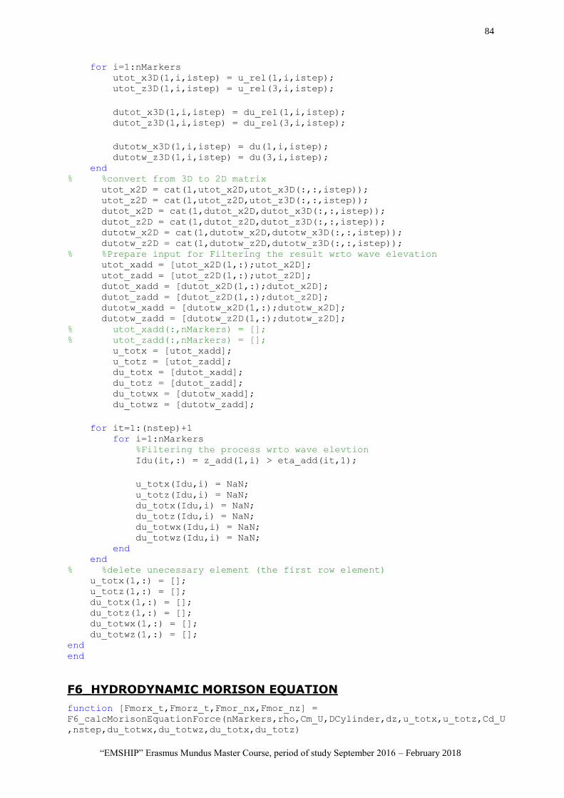
84
“EMSHIP” Erasmus Mundus Master Course, period of study September 2016 – February 2018
for i=1:nMarkers utot_x3D(1,i,istep) = u_rel(1,i,istep); utot_z3D(1,i,istep) = u_rel(3,i,istep);
dutot_x3D(1,i,istep) = du_rel(1,i,istep); dutot_z3D(1,i,istep) = du_rel(3,i,istep);
dutotw_x3D(1,i,istep) = du(1,i,istep); dutotw_z3D(1,i,istep) = du(3,i,istep); end % %convert from 3D to 2D matrix utot_x2D = cat(1,utot_x2D,utot_x3D(:,:,istep)); utot_z2D = cat(1,utot_z2D,utot_z3D(:,:,istep)); dutot_x2D = cat(1,dutot_x2D,dutot_x3D(:,:,istep)); dutot_z2D = cat(1,dutot_z2D,dutot_z3D(:,:,istep)); dutotw_x2D = cat(1,dutotw_x2D,dutotw_x3D(:,:,istep)); dutotw_z2D = cat(1,dutotw_z2D,dutotw_z3D(:,:,istep)); % %Prepare input for Filtering the result wrto wave elevation utot_xadd = [utot_x2D(1,:);utot_x2D]; utot_zadd = [utot_z2D(1,:);utot_z2D]; dutot_xadd = [dutot_x2D(1,:);dutot_x2D]; dutot_zadd = [dutot_z2D(1,:);dutot_z2D]; dutotw_xadd = [dutotw_x2D(1,:);dutotw_x2D]; dutotw_zadd = [dutotw_z2D(1,:);dutotw_z2D]; % utot_xadd(:,nMarkers) = []; % utot_zadd(:,nMarkers) = []; u_totx = [utot_xadd]; u_totz = [utot_zadd]; du_totx = [dutot_xadd]; du_totz = [dutot_zadd]; du_totwx = [dutotw_xadd]; du_totwz = [dutotw_zadd];
for it=1:(nstep)+1 for i=1:nMarkers %Filtering the process wrto wave elevtion Idu(it,:) = z_add(1,i) > eta_add(it,1);
u_totx(Idu,i) = NaN; u_totz(Idu,i) = NaN; du_totx(Idu,i) = NaN; du_totz(Idu,i) = NaN; du_totwx(Idu,i) = NaN; du_totwz(Idu,i) = NaN; end end % %delete unecessary element (the first row element) u_totx(1,:) = []; u_totz(1,:) = []; du_totx(1,:) = []; du_totz(1,:) = []; du_totwx(1,:) = []; du_totwz(1,:) = []; end end
F6_HYDRODYNAMIC MORISON EQUATION
function [Fmorx_t,Fmorz_t,Fmor_nx,Fmor_nz] =
F6_calcMorisonEquationForce(nMarkers,rho,Cm_U,DCylinder,dz,u_totx,u_totz,Cd_U
,nstep,du_totwx,du_totwz,du_totx,du_totz)
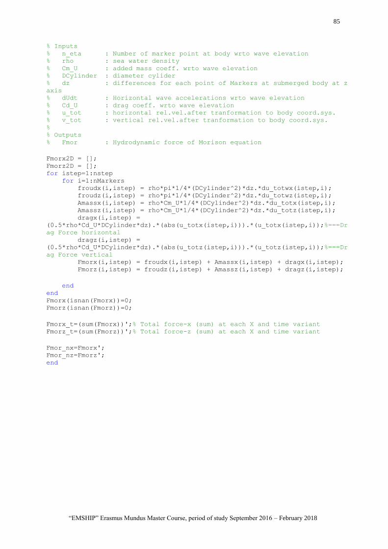
85
“EMSHIP” Erasmus Mundus Master Course, period of study September 2016 – February 2018
% Inputs % n_eta : Number of marker point at body wrto wave elevation % rho : sea water density % Cm_U : added mass coeff. wrto wave elevation % DCylinder : diameter cylider % dz : differences for each point of Markers at submerged body at z
axis % dUdt : Horizontal wave accelerations wrto wave elevation % Cd_U : drag coeff. wrto wave elevation % u_tot : horizontal rel.vel.after tranformation to body coord.sys. % v_tot : vertical rel.vel.after tranformation to body coord.sys. % % Outputs % Fmor : Hydrodynamic force of Morison equation
Fmorx2D = []; Fmorz2D = []; for istep=1:nstep for i=1:nMarkers froudx(i,istep) = rho*pi*1/4*(DCylinder^2)*dz.*du_totwx(istep,i); froudz(i,istep) = rho*pi*1/4*(DCylinder^2)*dz.*du_totwz(istep,i); Amassx(i,istep) = rho*Cm_U*1/4*(DCylinder^2)*dz.*du_totx(istep,i); Amassz(i,istep) = rho*Cm_U*1/4*(DCylinder^2)*dz.*du_totz(istep,i); dragx(i,istep) =
(0.5*rho*Cd_U*DCylinder*dz).*(abs(u_totx(istep,i))).*(u_totx(istep,i));%===Dr
ag Force horizontal dragz(i,istep) =
(0.5*rho*Cd_U*DCylinder*dz).*(abs(u_totz(istep,i))).*(u_totz(istep,i));%===Dr
ag Force vertical Fmorx(i,istep) = froudx(i,istep) + Amassx(i,istep) + dragx(i,istep); Fmorz(i,istep) = froudz(i,istep) + Amassz(i,istep) + dragz(i,istep);
end end Fmorx(isnan(Fmorx))=0; Fmorz(isnan(Fmorz))=0;
Fmorx_t=(sum(Fmorx))';% Total force-x (sum) at each X and time variant Fmorz_t=(sum(Fmorz))';% Total force-z (sum) at each X and time variant
Fmor_nx=Fmorx'; Fmor_nz=Fmorz'; end
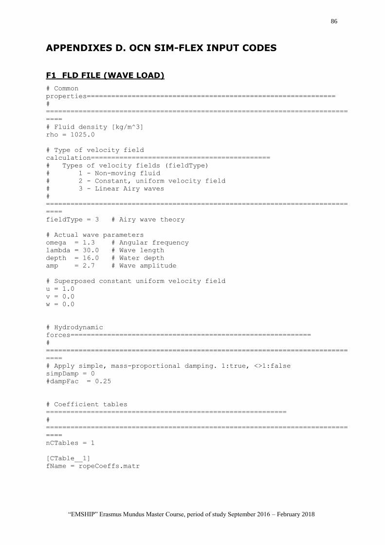
86
“EMSHIP” Erasmus Mundus Master Course, period of study September 2016 – February 2018
APPENDIXES D. OCN SIM-FLEX INPUT CODES
F1_FLD FILE (WAVE LOAD)
# Common
properties=============================================================
#
==========================================================================
====
# Fluid density [kg/m^3]
rho = 1025.0
# Type of velocity field
calculation============================================
# Types of velocity fields (fieldType)
# 1 - Non-moving fluid
# 2 - Constant, uniform velocity field
# 3 - Linear Airy waves
#
==========================================================================
====
fieldType = 3 # Airy wave theory
# Actual wave parameters
omega = 1.3 # Angular frequency
lambda = 30.0 # Wave length
depth = 16.0 # Water depth
amp = 2.7 # Wave amplitude
# Superposed constant uniform velocity field
u = 1.0
v = 0.0
w = 0.0
# Hydrodynamic
forces===========================================================
#
==========================================================================
====
# Apply simple, mass-proportional damping. 1:true, <>1:false
simpDamp = 0
#dampFac = 0.25
# Coefficient tables
===========================================================
#
==========================================================================
====
nCTables = 1
[CTable__1]
fName = ropeCoeffs.matr
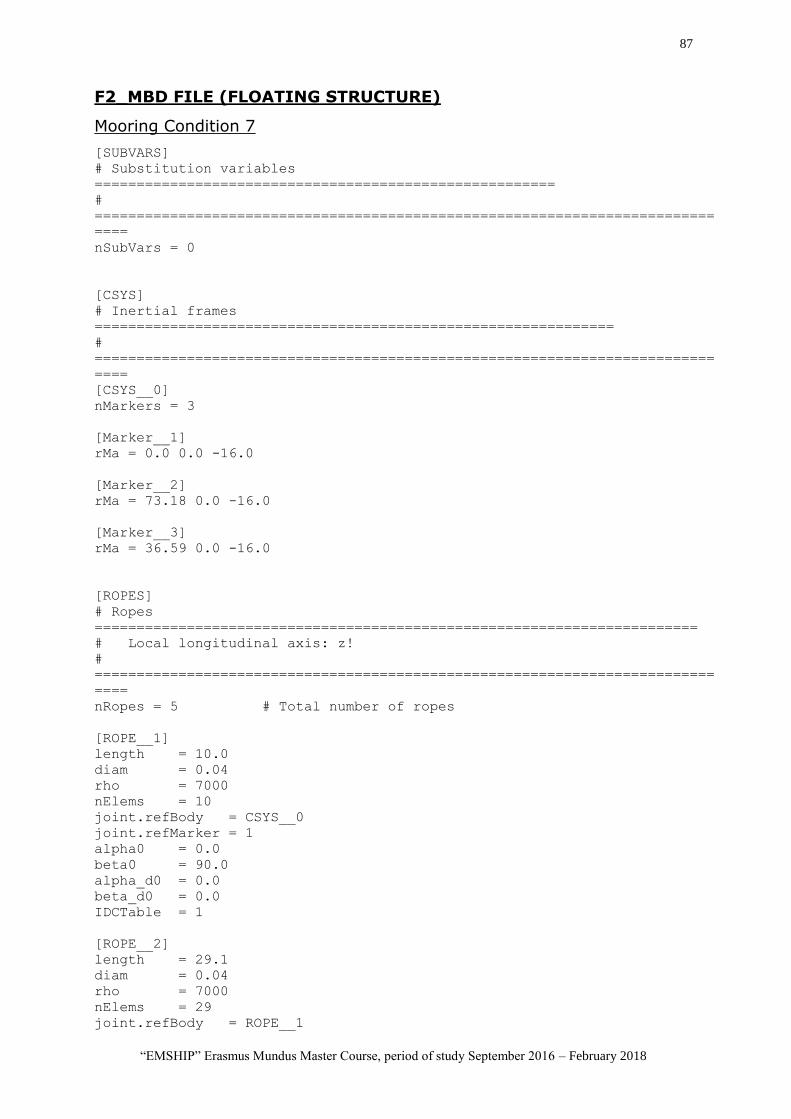
87
“EMSHIP” Erasmus Mundus Master Course, period of study September 2016 – February 2018
F2_MBD FILE (FLOATING STRUCTURE)
Mooring Condition 7
[SUBVARS]
# Substitution variables
=======================================================
#
==========================================================================
====
nSubVars = 0
[CSYS]
# Inertial frames
==============================================================
#
==========================================================================
====
[CSYS__0]
nMarkers = 3
[Marker__1]
rMa = 0.0 0.0 -16.0
[Marker__2]
rMa = 73.18 0.0 -16.0
[Marker__3]
rMa = 36.59 0.0 -16.0
[ROPES]
# Ropes
========================================================================
# Local longitudinal axis: z!
#
==========================================================================
====
nRopes = 5 # Total number of ropes
[ROPE__1]
length = 10.0
diam = 0.04
rho = 7000
nElems = 10
joint.refBody = CSYS__0
joint.refMarker = 1
alpha0 = 0.0
beta0 = 90.0
alpha_d0 = 0.0
beta_d0 = 0.0
IDCTable = 1
[ROPE__2]
length = 29.1
diam = 0.04
rho = 7000
nElems = 29
joint.refBody = ROPE__1
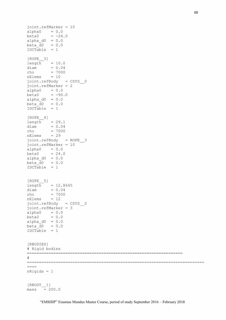
88
“EMSHIP” Erasmus Mundus Master Course, period of study September 2016 – February 2018
joint.refMarker = 10
alpha0 = 0.0
beta0 = -24.0
alpha_d0 = 0.0
beta_d0 = 0.0
IDCTable = 1
[ROPE__3]
length = 10.0
diam = 0.04
rho = 7000
nElems = 10
joint.refBody = CSYS__0
joint.refMarker = 2
alpha0 = 0.0
beta0 = -90.0
alpha_d0 = 0.0
beta_d0 = 0.0
IDCTable = 1
[ROPE__4]
length = 29.1
diam = 0.04
rho = 7000
nElems = 29
joint.refBody = ROPE__3
joint.refMarker = 10
alpha0 = 0.0
beta0 = 24.0
alpha_d0 = 0.0
beta_d0 = 0.0
IDCTable = 1
[ROPE__5]
length = 12.8645
diam = 0.04
rho = 7000
nElems = 12
joint.refBody = CSYS__0
joint.refMarker = 3
alpha0 = 0.0
beta0 = 0.0
alpha_d0 = 0.0
beta_d0 = 0.0
IDCTable = 1
[RBODIES]
# Rigid bodies
=================================================================
#
==========================================================================
====
nRigids = 1
[RBODY__1]
mass = 200.0
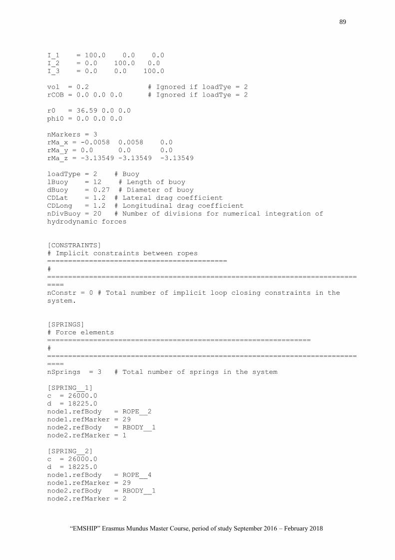
89
“EMSHIP” Erasmus Mundus Master Course, period of study September 2016 – February 2018
I_1 = 100.0 0.0 0.0
I_2 = 0.0 100.0 0.0
I_3 = 0.0 0.0 100.0
vol = 0.2 # Ignored if loadTye = 2
rCOB = 0.0 0.0 0.0 # Ignored if loadTye = 2
r0 = 36.59 0.0 0.0
phi0 = 0.0 0.0 0.0
nMarkers = 3
rMa_x = -0.0058 0.0058 0.0
rMa_y = 0.0 0.0 0.0
rMa_z = -3.13549 -3.13549 -3.13549
loadType = 2 # Buoy
lBuoy = 12 # Length of buoy
dBuoy = 0.27 # Diameter of buoy
CDLat = 1.2 # Lateral drag coefficient
CDLong = 1.2 # Longitudinal drag coefficient
nDivBuoy = 20 # Number of divisions for numerical integration of
hydrodynamic forces
[CONSTRAINTS]
# Implicit constraints between ropes
===========================================
#
==========================================================================
====
nConstr = 0 # Total number of implicit loop closing constraints in the
system.
[SPRINGS]
# Force elements
===============================================================
#
==========================================================================
====
nSprings = 3 # Total number of springs in the system
[SPRING__1]
c = 26000.0
d = 18225.0
node1.refBody = ROPE__2
node1.refMarker = 29
node2.refBody = RBODY__1
node2.refMarker = 1
[SPRING__2]
c = 26000.0
d = 18225.0
node1.refBody = ROPE__4
node1.refMarker = 29
node2.refBody = RBODY__1
node2.refMarker = 2
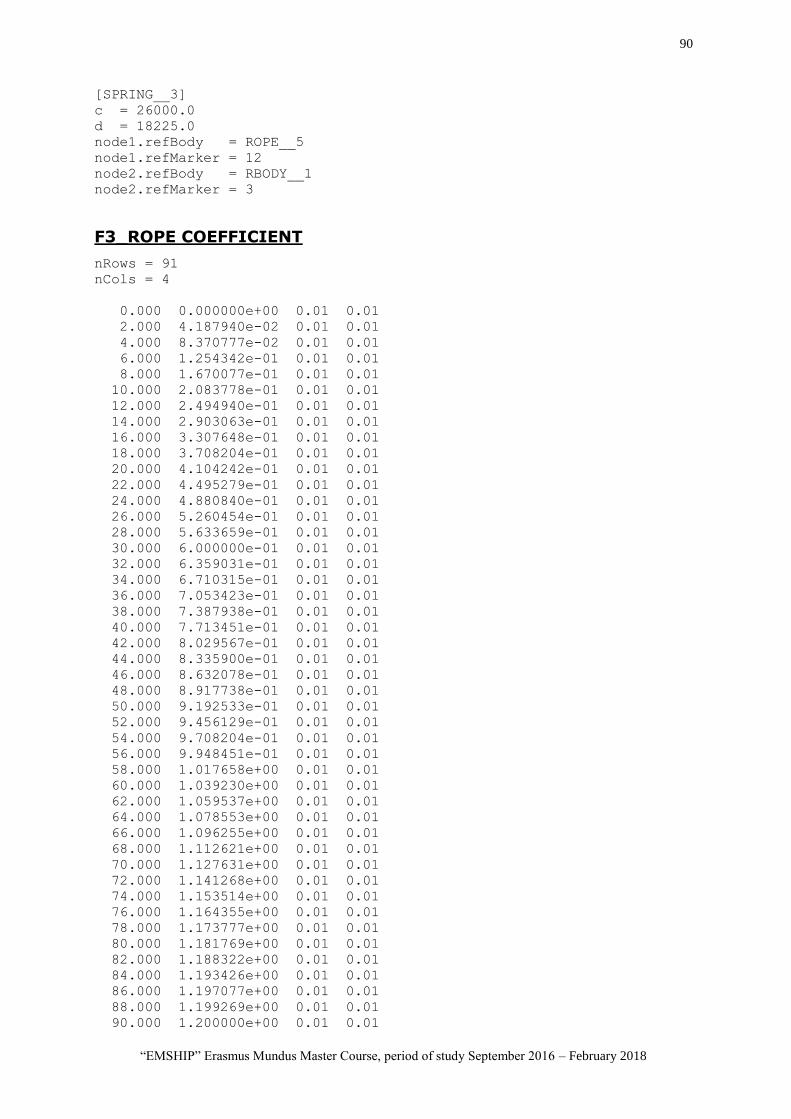
90
“EMSHIP” Erasmus Mundus Master Course, period of study September 2016 – February 2018
[SPRING__3]
c = 26000.0
d = 18225.0
node1.refBody = ROPE__5
node1.refMarker = 12
node2.refBody = RBODY__1
node2.refMarker = 3
F3_ROPE COEFFICIENT
nRows = 91
nCols = 4
0.000 0.000000e+00 0.01 0.01
2.000 4.187940e-02 0.01 0.01
4.000 8.370777e-02 0.01 0.01
6.000 1.254342e-01 0.01 0.01
8.000 1.670077e-01 0.01 0.01
10.000 2.083778e-01 0.01 0.01
12.000 2.494940e-01 0.01 0.01
14.000 2.903063e-01 0.01 0.01
16.000 3.307648e-01 0.01 0.01
18.000 3.708204e-01 0.01 0.01
20.000 4.104242e-01 0.01 0.01
22.000 4.495279e-01 0.01 0.01
24.000 4.880840e-01 0.01 0.01
26.000 5.260454e-01 0.01 0.01
28.000 5.633659e-01 0.01 0.01
30.000 6.000000e-01 0.01 0.01
32.000 6.359031e-01 0.01 0.01
34.000 6.710315e-01 0.01 0.01
36.000 7.053423e-01 0.01 0.01
38.000 7.387938e-01 0.01 0.01
40.000 7.713451e-01 0.01 0.01
42.000 8.029567e-01 0.01 0.01
44.000 8.335900e-01 0.01 0.01
46.000 8.632078e-01 0.01 0.01
48.000 8.917738e-01 0.01 0.01
50.000 9.192533e-01 0.01 0.01
52.000 9.456129e-01 0.01 0.01
54.000 9.708204e-01 0.01 0.01
56.000 9.948451e-01 0.01 0.01
58.000 1.017658e+00 0.01 0.01
60.000 1.039230e+00 0.01 0.01
62.000 1.059537e+00 0.01 0.01
64.000 1.078553e+00 0.01 0.01
66.000 1.096255e+00 0.01 0.01
68.000 1.112621e+00 0.01 0.01
70.000 1.127631e+00 0.01 0.01
72.000 1.141268e+00 0.01 0.01
74.000 1.153514e+00 0.01 0.01
76.000 1.164355e+00 0.01 0.01
78.000 1.173777e+00 0.01 0.01
80.000 1.181769e+00 0.01 0.01
82.000 1.188322e+00 0.01 0.01
84.000 1.193426e+00 0.01 0.01
86.000 1.197077e+00 0.01 0.01
88.000 1.199269e+00 0.01 0.01
90.000 1.200000e+00 0.01 0.01
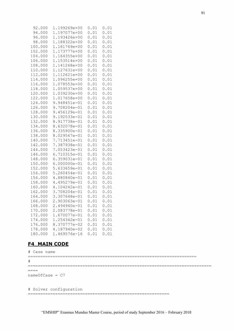
91
“EMSHIP” Erasmus Mundus Master Course, period of study September 2016 – February 2018
92.000 1.199269e+00 0.01 0.01
94.000 1.197077e+00 0.01 0.01
96.000 1.193426e+00 0.01 0.01
98.000 1.188322e+00 0.01 0.01
100.000 1.181769e+00 0.01 0.01
102.000 1.173777e+00 0.01 0.01
104.000 1.164355e+00 0.01 0.01
106.000 1.153514e+00 0.01 0.01
108.000 1.141268e+00 0.01 0.01
110.000 1.127631e+00 0.01 0.01
112.000 1.112621e+00 0.01 0.01
114.000 1.096255e+00 0.01 0.01
116.000 1.078553e+00 0.01 0.01
118.000 1.059537e+00 0.01 0.01
120.000 1.039230e+00 0.01 0.01
122.000 1.017658e+00 0.01 0.01
124.000 9.948451e-01 0.01 0.01
126.000 9.708204e-01 0.01 0.01
128.000 9.456129e-01 0.01 0.01
130.000 9.192533e-01 0.01 0.01
132.000 8.917738e-01 0.01 0.01
134.000 8.632078e-01 0.01 0.01
136.000 8.335900e-01 0.01 0.01
138.000 8.029567e-01 0.01 0.01
140.000 7.713451e-01 0.01 0.01
142.000 7.387938e-01 0.01 0.01
144.000 7.053423e-01 0.01 0.01
146.000 6.710315e-01 0.01 0.01
148.000 6.359031e-01 0.01 0.01
150.000 6.000000e-01 0.01 0.01
152.000 5.633659e-01 0.01 0.01
154.000 5.260454e-01 0.01 0.01
156.000 4.880840e-01 0.01 0.01
158.000 4.495279e-01 0.01 0.01
160.000 4.104242e-01 0.01 0.01
162.000 3.708204e-01 0.01 0.01
164.000 3.307648e-01 0.01 0.01
166.000 2.903063e-01 0.01 0.01
168.000 2.494940e-01 0.01 0.01
170.000 2.083778e-01 0.01 0.01
172.000 1.670077e-01 0.01 0.01
174.000 1.254342e-01 0.01 0.01
176.000 8.370777e-02 0.01 0.01
178.000 4.187940e-02 0.01 0.01
180.000 1.469576e-16 0.01 0.01
F4_MAIN CODE
# Case name
====================================================================
#
==========================================================================
====
nameOfCase = C7
# Solver configuration
=========================================================
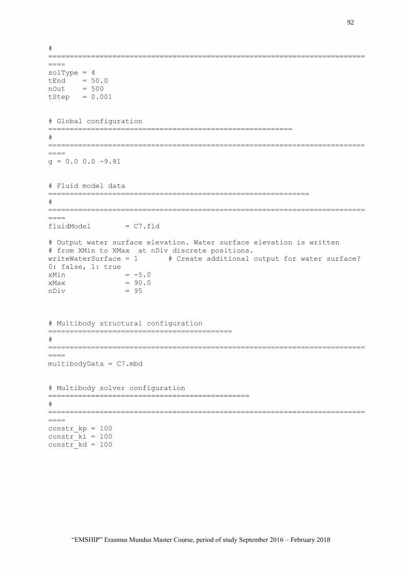
92
“EMSHIP” Erasmus Mundus Master Course, period of study September 2016 – February 2018
#
==========================================================================
====
solType = 4
tEnd = 50.0
nOut = 500
tStep = 0.001
# Global configuration
=========================================================
#
==========================================================================
====
g = 0.0 0.0 -9.81
# Fluid model data
=============================================================
#
==========================================================================
====
fluidModel = C7.fld
# Output water surface elevation. Water surface elevation is written
# from XMin to XMax at nDiv discrete positions.
writeWaterSurface = 1 # Create additional output for water surface?
0: false, 1: true
xMin = -5.0
xMax = 90.0
nDiv = 95
# Multibody structural configuration
===========================================
#
==========================================================================
====
multibodyData = C7.mbd
# Multibody solver configuration
===============================================
#
==========================================================================
====
constr_kp = 100
constr_ki = 100
constr_kd = 100