compara˘c~ao do desempenho de arquiteturas h bridas para
TRANSCRIPT

Universidade de AveiroDepartamento deEletronica, Telecomunicacoes e Informatica,
2016
Daniel FilipePinheiro de Azevedo
Comparacao do desempenho de ArquiteturasHıbridas para comunicacoes na banda das ondasmilimetricas
Performance comparison of Hybrid Architecturesfor millimeter wave communications


Universidade de AveiroDepartamento deEletronica, Telecomunicacoes e Informatica,
2016
Daniel FilipePinheiro de Azevedo
Comparacao do desempenho de ArquiteturasHıbridas para comunicacoes na banda das ondasmilimetricas
Performance comparison of Hybrid Architecturesfor millimeter wave communications
Dissertacao apresentada a Universidade de Aveiro para cumprimento dos re-quesitos necessarios a obtencao do grau de Mestre em Engenharia Eletronicae Telecomunicacoes, realizada sob a orientacao cientıfica do ProfessorDoutor Adao Silva (orientador), Professor auxiliar do Departamento deEletronica, Telecomunicacoes e Informatica da Universidade de Aveiro edo Doutor Daniel Castanheira (co-orientador), investigador no Instituto deTelecomunicacoes de Aveiro.


o juri / the jury
presidente / president Professor Doutor Jose Carlos Esteves Duarte PedroProfessor Catedratico da Universidade de Aveiro
vogais / examiners committee Professor Doutor Paulo Jorge Coelho MarquesProfessor Adjunto no Instituto Politecnico de Castelo Branco
Professor Doutor Adao Paulo Soares da SilvaProfessor Auxiliar na Universidade de Aveiro


agradecimentos Queria deixar um agradecimento a todas as pessoas sem as quais nao teriasido possıvel concluir este trajecto.
E principalmente,
A minha famılia, aos meus pais, avos, irma e madrinha, por todo o apoioe a ajuda ao longo destes anos, sem o qual este objetivo nao teria sidoconcluıdo.
Aos professores, Adao Silva e Daniel Castanheira por toda a ajuda, ori-entacao, e disponibilidade demonstrada ao longo deste ano.
Aos meus amigos, por toda amizade, paciencia e tolerancia demonstradaao longo destes anos, principalmente nos meus perıodos de ausencia.
A todos um enorme Muito Obrigado.


Palavras-chave 5G, mmWave communications, massive MIMO, hybrid analog/digital archi-tectures
Resumo A proliferacao massiva das comunicacoes sem fios faz prever que onumero de utilizadores aumente exponencialmente ate 2020, o que tornaranecessario um suporte de trafego milhares de vezes superior e com ligacoesna ordem dos Gigabit por segundo. Este incremento exigira um aumento sig-nificativo da eficiencia espectral e energetica. Impoe-se portanto, uma mu-danca de paradigma dos sistemas de comunicacao sem fios convencionais,imposta pela introducao da 5a geracao.
Para o efeito, e necessario desenvolver novas e promissoras tecnicas detransmissao, nomeadamente a utilizacao de ondas milimetricas em sistemascom um numero massivo de antenas. No entanto, consideraveis desafiosemergem ao adotar estas tecnicas. Por um lado, este tipo de ondas sofregrandes dificuldades em termos de propagacao. Por outro lado, a adocaode arquiteturas convencionais para sistemas com um numero massivo deantenas e absolutamente inviavel, devido ao custo e ao nıvel de complexi-dade inerentes. Isto acontece porque o processamento de sinal ao nıvel dacamada fısica e maioritariamente feito em banda base, ou seja, no domıniodigital requerendo uma cadeia RF por cada antena.
Neste contexto as arquiteturas hıbridas sao uma proposta relativamenterecente que visa simplificar a utilizacao de um grande numero de antenas,dividindo o processamento entre os domınios analogico e digital. Para alemdisso, o numero de cadeias RF necessarias e bastante inferior ao numerototal de antenas do sistema, contribuindo para obvias melhorias em termosde complexidade, custo e energia consumida.
Nesta dissertacao e implementada uma arquitetura hıbrida para ondasmilimetricas, onde cada cadeia RF esta apenas conectada a um pequenoconjunto de antenas. E considerado um sistema contendo um transmissore um recetor ambos equipados com um grande numero de antenas e onde,o numero de cadeias RF e bastante inferior ao numero total de antenas.Pre-codificadores hıbridos analogico/digital, recentemente propostos na lit-eratura sao utilizados e novos equalizadores hıbridos analogico/digital saoprojetados. E feita uma avaliacao de performance a arquitetura implemen-tada e posteriormente comparada com uma outra arquitetura, onde todasas antenas estao conectadas a todas as cadeias RF.

Keywords 5G, mmWave communications, massive MIMO, hybrid analog/digital archi-tectures
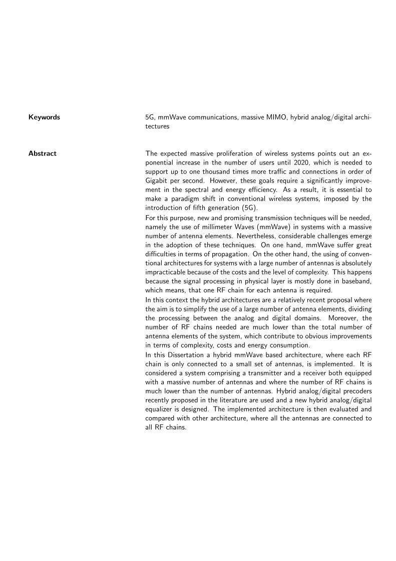
Abstract The expected massive proliferation of wireless systems points out an ex-ponential increase in the number of users until 2020, which is needed tosupport up to one thousand times more traffic and connections in order ofGigabit per second. However, these goals require a significantly improve-ment in the spectral and energy efficiency. As a result, it is essential tomake a paradigm shift in conventional wireless systems, imposed by theintroduction of fifth generation (5G).
For this purpose, new and promising transmission techniques will be needed,namely the use of millimeter Waves (mmWave) in systems with a massivenumber of antenna elements. Nevertheless, considerable challenges emergein the adoption of these techniques. On one hand, mmWave suffer greatdifficulties in terms of propagation. On the other hand, the using of conven-tional architectures for systems with a large number of antennas is absolutelyimpracticable because of the costs and the level of complexity. This happensbecause the signal processing in physical layer is mostly done in baseband,which means, that one RF chain for each antenna is required.
In this context the hybrid architectures are a relatively recent proposal wherethe aim is to simplify the use of a large number of antenna elements, dividingthe processing between the analog and digital domains. Moreover, thenumber of RF chains needed are much lower than the total number ofantenna elements of the system, which contribute to obvious improvementsin terms of complexity, costs and energy consumption.
In this Dissertation a hybrid mmWave based architecture, where each RFchain is only connected to a small set of antennas, is implemented. It isconsidered a system comprising a transmitter and a receiver both equippedwith a massive number of antennas and where the number of RF chains ismuch lower than the number of antennas. Hybrid analog/digital precodersrecently proposed in the literature are used and a new hybrid analog/digitalequalizer is designed. The implemented architecture is then evaluated andcompared with other architecture, where all the antennas are connected toall RF chains.


Contents
Contents i
List of Figures iii
List of Tables v
Acronyms vii
1 Introduction 1
1.1 Mobile Communications Evolution . . . . . . . . . . . . . . . . . . . . . . . . 1
1.2 Towards 5G systems . . . . . . . . . . . . . . . . . . . . . . . . . . . . . . . . 6
1.3 Motivation and Objectives . . . . . . . . . . . . . . . . . . . . . . . . . . . . . 7
1.4 Contributions . . . . . . . . . . . . . . . . . . . . . . . . . . . . . . . . . . . . 9
1.5 Outline . . . . . . . . . . . . . . . . . . . . . . . . . . . . . . . . . . . . . . . 9
1.6 Notation . . . . . . . . . . . . . . . . . . . . . . . . . . . . . . . . . . . . . . . 10
2 MIMO Systems 11
2.1 Multiple Antenna Schemes . . . . . . . . . . . . . . . . . . . . . . . . . . . . . 11
2.2 Diversity . . . . . . . . . . . . . . . . . . . . . . . . . . . . . . . . . . . . . . . 13
2.2.1 Receive Diversity . . . . . . . . . . . . . . . . . . . . . . . . . . . . . . 15
Maximal Ratio Combining . . . . . . . . . . . . . . . . . . . . . . . . . 17
Equal Gain Combining . . . . . . . . . . . . . . . . . . . . . . . . . . . 17
Selection Combining . . . . . . . . . . . . . . . . . . . . . . . . . . . . 18
2.2.2 Transmit Diversity . . . . . . . . . . . . . . . . . . . . . . . . . . . . . 18
Closed loop . . . . . . . . . . . . . . . . . . . . . . . . . . . . . . . . . 18
Open loop . . . . . . . . . . . . . . . . . . . . . . . . . . . . . . . . . . 19
2.3 Spatial Multiplexing . . . . . . . . . . . . . . . . . . . . . . . . . . . . . . . . 21
2.3.1 SU-MIMO Techniques for Spatial Multiplexing . . . . . . . . . . . . . 22
Channel known at the transmitter . . . . . . . . . . . . . . . . . . . . 22
Channel known only at the receiver . . . . . . . . . . . . . . . . . . . 25
2.3.2 MU-MIMO Techniques for Spatial Multiplexing . . . . . . . . . . . . . 26
2.4 Beamforming . . . . . . . . . . . . . . . . . . . . . . . . . . . . . . . . . . . . 27
3 Millimeter Wave and Massive MIMO Systems 29
3.1 Millimeter Waves . . . . . . . . . . . . . . . . . . . . . . . . . . . . . . . . . . 29
3.2 Massive MIMO . . . . . . . . . . . . . . . . . . . . . . . . . . . . . . . . . . . 32
3.3 Massive Beamforming . . . . . . . . . . . . . . . . . . . . . . . . . . . . . . . 34
i

3.3.1 Antenna Designs . . . . . . . . . . . . . . . . . . . . . . . . . . . . . . 343.4 Architectures for mmWave mMIMO Systems . . . . . . . . . . . . . . . . . . 36
3.4.1 Full-array architecture . . . . . . . . . . . . . . . . . . . . . . . . . . . 373.4.2 Sub-array architecture . . . . . . . . . . . . . . . . . . . . . . . . . . . 383.4.3 1-bit ADC architecture . . . . . . . . . . . . . . . . . . . . . . . . . . 38
3.5 Millimeter Wave MIMO channel . . . . . . . . . . . . . . . . . . . . . . . . . 393.5.1 Types of channels . . . . . . . . . . . . . . . . . . . . . . . . . . . . . 39
CBSM . . . . . . . . . . . . . . . . . . . . . . . . . . . . . . . . . . . . 39GBSM . . . . . . . . . . . . . . . . . . . . . . . . . . . . . . . . . . . . 40PSM . . . . . . . . . . . . . . . . . . . . . . . . . . . . . . . . . . . . . 40
3.5.2 Millimeter Wave MIMO Channel model . . . . . . . . . . . . . . . . . 413.6 Small Cell Networks . . . . . . . . . . . . . . . . . . . . . . . . . . . . . . . . 42
3.6.1 Cell Types . . . . . . . . . . . . . . . . . . . . . . . . . . . . . . . . . 43
4 Architectures and Processing Techniques for mmWave mMIMO Systems 454.1 System Characterization . . . . . . . . . . . . . . . . . . . . . . . . . . . . . . 464.2 MmWave mMIMO Architecture 1 . . . . . . . . . . . . . . . . . . . . . . . . 47
4.2.1 Transmitter Model Description . . . . . . . . . . . . . . . . . . . . . . 474.2.2 Receiver Model Description . . . . . . . . . . . . . . . . . . . . . . . . 484.2.3 Algorithm Description . . . . . . . . . . . . . . . . . . . . . . . . . . . 48
Hybrid Analog/Digital Precoding . . . . . . . . . . . . . . . . . . . . . 49Hybrid Analog/Digital Combining . . . . . . . . . . . . . . . . . . . . 50
4.3 MmWave mMIMO Architecture 2 . . . . . . . . . . . . . . . . . . . . . . . . 514.3.1 Transmitter Model Description . . . . . . . . . . . . . . . . . . . . . . 524.3.2 Receiver Model Description . . . . . . . . . . . . . . . . . . . . . . . . 534.3.3 Algorithm Description . . . . . . . . . . . . . . . . . . . . . . . . . . . 54
Hybrid Analog/Digital Precoding . . . . . . . . . . . . . . . . . . . . . 54Hybrid Analog/Digital Combining . . . . . . . . . . . . . . . . . . . . 55
4.4 Performance Results . . . . . . . . . . . . . . . . . . . . . . . . . . . . . . . . 564.4.1 Scenario 1 . . . . . . . . . . . . . . . . . . . . . . . . . . . . . . . . . . 584.4.2 Scenario 2 . . . . . . . . . . . . . . . . . . . . . . . . . . . . . . . . . . 604.4.3 Scenario 3 . . . . . . . . . . . . . . . . . . . . . . . . . . . . . . . . . . 62
5 Conclusions and Future Work 655.1 Conclusions . . . . . . . . . . . . . . . . . . . . . . . . . . . . . . . . . . . . . 655.2 Future Work . . . . . . . . . . . . . . . . . . . . . . . . . . . . . . . . . . . . 66
Bibliography 67
ii
List of Figures
1.1 Cellular Technology Evolution . . . . . . . . . . . . . . . . . . . . . . . . . . . 2
1.2 Global Mobile Subscribers and Market Shares . . . . . . . . . . . . . . . . . . 3
1.3 Annual Global Technology Forecast Subscriptions & Market Share 2016-2020 5
1.4 5G service and scenario requirements . . . . . . . . . . . . . . . . . . . . . . . 7
2.1 SISO configuration . . . . . . . . . . . . . . . . . . . . . . . . . . . . . . . . . 12
2.2 SIMO configuration . . . . . . . . . . . . . . . . . . . . . . . . . . . . . . . . 12
2.3 MISO configuration . . . . . . . . . . . . . . . . . . . . . . . . . . . . . . . . 12
2.4 MIMO configuration . . . . . . . . . . . . . . . . . . . . . . . . . . . . . . . . 13
2.5 Time and Frequency Diversity . . . . . . . . . . . . . . . . . . . . . . . . . . . 14
2.6 Reducing fading by using a combination of two uncorrelated signals . . . . . 15
2.7 Spatial receive antenna diversity . . . . . . . . . . . . . . . . . . . . . . . . . 16
2.8 Alamouti technique for open loop transmit diversity . . . . . . . . . . . . . . 19
2.9 Alamouti receiver block diagram . . . . . . . . . . . . . . . . . . . . . . . . . 20
2.10 Spatial multiplexing in a MIMO System . . . . . . . . . . . . . . . . . . . . . 22
2.11 Water Filling power scheme . . . . . . . . . . . . . . . . . . . . . . . . . . . . 24
2.12 Performance comparison between the different equalizers . . . . . . . . . . . . 26
2.13 Uplink MU-MIMO transmissions . . . . . . . . . . . . . . . . . . . . . . . . . 27
2.14 Beamforming technique . . . . . . . . . . . . . . . . . . . . . . . . . . . . . . 27
3.1 Atmospheric absorption across mmWave frequencies in dB/Km . . . . . . . . 31
3.2 Antenna Array configurations mMIMO . . . . . . . . . . . . . . . . . . . . . . 33
3.3 Comparison antennas at different frequencies with the same dimensions . . . 34
3.4 Hybrid Antenna Arrays . . . . . . . . . . . . . . . . . . . . . . . . . . . . . . 35
3.5 Antenna Front-End Integration . . . . . . . . . . . . . . . . . . . . . . . . . . 36
3.6 Hybrid BF: Full-array architecture . . . . . . . . . . . . . . . . . . . . . . . . 37
3.7 Hybrid BF: Sub-array architecture . . . . . . . . . . . . . . . . . . . . . . . . 38
3.8 Hybrid BF: 1-bit ADC architecture . . . . . . . . . . . . . . . . . . . . . . . . 38
3.9 HetNet utilizing a mix of macro, pico, femto and relay BS . . . . . . . . . . . 42
4.1 Transmitter block diagram for HA-1 . . . . . . . . . . . . . . . . . . . . . . . 47
4.2 Receiver block diagram for HA-1 . . . . . . . . . . . . . . . . . . . . . . . . . 48
4.3 Diagram of the proposed iterative hybrid analog/digital precoding . . . . . . 52
4.4 Transmitter block diagram for HA-2 . . . . . . . . . . . . . . . . . . . . . . . 52
4.5 Receiver block diagram for HA-2 . . . . . . . . . . . . . . . . . . . . . . . . . 53
4.6 Performance of the proposed hybrid equalizer as a function of time slots (T )for HA-1 and Scenario 3 . . . . . . . . . . . . . . . . . . . . . . . . . . . . . . 57
iii

4.7 Performance comparison of both architectures considering hybrid random pre-coders, for Scenario 1 . . . . . . . . . . . . . . . . . . . . . . . . . . . . . . . . 58
4.8 Performance comparison of both architectures considering hybrid precoders,for Scenario 1 . . . . . . . . . . . . . . . . . . . . . . . . . . . . . . . . . . . . 59
4.9 BER performance as a function of the number of transmit antennas consideringhybrid precoders, for Scenario 1 . . . . . . . . . . . . . . . . . . . . . . . . . . 59
4.10 Performance comparison of both architectures considering hybrid random pre-coders, for Scenario 2 . . . . . . . . . . . . . . . . . . . . . . . . . . . . . . . . 60
4.11 Performance comparison of both architectures considering hybrid precoders,for Scenario 2 . . . . . . . . . . . . . . . . . . . . . . . . . . . . . . . . . . . . 61
4.12 BER performance as a function of the number of RF chains considering hybridrandom precoders, for Scenario 2 . . . . . . . . . . . . . . . . . . . . . . . . . 61
4.13 Performance comparison of both architectures considering hybrid random pre-coders, for Scenario 3 . . . . . . . . . . . . . . . . . . . . . . . . . . . . . . . . 62
4.14 Performance comparison of both architectures considering hybrid precoders,for Scenario 3 . . . . . . . . . . . . . . . . . . . . . . . . . . . . . . . . . . . . 63
iv
List of Tables
2.1 STBC - TSTD mapping . . . . . . . . . . . . . . . . . . . . . . . . . . . . . . 21
3.1 Signal Loss through Atmosphere . . . . . . . . . . . . . . . . . . . . . . . . . 313.2 Characteristics of the different base stations . . . . . . . . . . . . . . . . . . . 44
4.1 Precoder algorithm for HA-1 . . . . . . . . . . . . . . . . . . . . . . . . . . . 494.2 Combining algorithm for HA-1 . . . . . . . . . . . . . . . . . . . . . . . . . . 514.3 Precoder algorithm for HA-2 . . . . . . . . . . . . . . . . . . . . . . . . . . . 554.4 Combining algorithm for HA-2 . . . . . . . . . . . . . . . . . . . . . . . . . . 564.5 General parameters of the different scenarios . . . . . . . . . . . . . . . . . . 57
v

vi

List of Acronyms
1G 1st Generation
2D Two Dimensional
2G 2nd Generation
3D Three Dimensional
3G 3rd Generation
3GPP Third-Generation Partnership Project
4G 4th Generation
5G 5th Generation
AA Antenna Array
ADC Analogue to Digital Converter
AoA Angle of Arrival
AoD Angle of Departure
AWGN Added White Gaussian Noise
BER Bit Error Ratio
BS Base Station
CBSM Correlation-Based Stochastic Model
CoMP Coordinated Multipoint
CSI Channel State Information
DDCM Double Directional Channel Model
DoF Degrees of Freedom
EDGE Enhanced Data Rate for Global Evolution
EE Energy Efficiency
EGC Equal Gain Combining
eNB evolved Node B
FCC Federal Communications Commission
FDD Frequency Division Duplex
FDD-TDD CA Frequency Division Duplex - Time Division Duplex Carrier Aggregation
FDMA Frequency Division Multiple Access
vii
GBSM Geometry-Based Stochastic Model
GPRS General Packet Radio Service
GSM Global System for Mobile Communications
HA-1 Hybrid Architecture 1
HA-2 Hybrid Architecture 2
HetNets Heterogeneous Networks
HSDCSD High-Speed Circuit Switched Data
HSDPA High Speed Downlink Packet Access
HSPA High Speed Packet Access
HSUPA High Speed Uplink Packet Access
i.i.d. independent identically distributed
IMT-Advanced International Mobile Telecommunications Advanced
ITU-R International Telecommunications Union Radiocommunication Sector
IEEE Institute of Electrical and Electronics Engineers
LNA Low Noise Amplifiers
LoS Line-of-Sight
LTE Long Term Evolution
MBMS Multimedia Broadcast/Multimedia Services
MIMO Multiple-Input Multiple-Output
MISO Multiple-Input Single-Output
MIT Massachusetts Institute of Technology
mMIMO massive Multiple-Input Multiple-Output
MMIC Monolithic Microwave Integrated Circuits
MMS Multimedia Message Services
MMSE Minimum Mean Square Error
mmWave Millimeter Wave
MRC Maximal Ratio Combining
MTC Massive machine-type communication
MU-MIMO Multi-user MIMO
viii

NLoS Non-Line-of-Sight
OFDM Orthogonal Frequency Division Multiplexing
OFDMA Orthogonal Frequency Division Multiple Access
PA Power Amplifiers
PIC Parallel Interference Cancellation
PMI Precoding Matrix Indicator
ProSe Proximity Services
PSM Parametric Stochastic Model
QAM Quadrature Amplitude Modulation
QoS Quality of Service
RF Radio Frequency
SC Selection Combining
SC-FDMA Single Carrier Frequency Division Multiple Access
SCN Small Cell Network
SE spectral efficiency
SFBC Space-frequency Block Code
SIC Successive Interference Cancellation
SIMO Single-Input Multiple-Output
SISO Single-Input Single-Output
SNR Signal-to-Noise Ratio
STBC Space-time Block Code
STBC - TSTD STBC - Time Shift Transmit Diversity
SU-MIMO Single-User MIMO
SVD Singular Value Decomposition
TDD Time Division Duplex
TDMA Time Division Multiple Access
UE User Equipment
ULA Uniform Linear Array
UMTS Universal Mobile Telecommunication System
ix

UPA Uniform Planar Array
UWB Ultra-Wideband
VRM Virtual Ray Model
WCDMA Wideband Code-Division Multiple Access
WiMAX Worldwide Interoperability for Microwave Access
ZF Zero-Forcing
x

Chapter 1
Introduction
This dissertation begins with an introduction to the technologies used in the developmentsof the implemented work. To easily understand the technologies, this chapter starts with anevolution of the mobile communications system since their beginning until the used systemsnowadays. The future deployments, are described in the next sections. Then the motivations,objectives and the main contributions are presented. Finally, a brief summary of the followingchapters is made.
1.1 Mobile Communications Evolution
The technology or concept of wireless technology is not recent. In fact, the story of wirelessphones is dated way back to the middle of the 20th century [1]. The world first mobile phonecall was made on April 3, 1973, when Martin Cooper, a senior engineer at Motorola, calleda rival telecommunications company and informed them that he was speaking via a mobilephone [2]. Since those days a lot innovations have been made and the perception of mobilephones changed.
At the beginning, they were considered just luxury items although nowadays they arean important instrument in our lives. The newest, sleek phones support mobile customersby providing applications in communication, navigation, multimedia, entertainment amongothers. Once perceived as luxury items, cell phones have become a necessity for many [3].A recent Massachusetts Institute of Technology (MIT) survey, listed cell phones as the mosthated invention that Americans cannot live without, even more so than alarm clocks, televi-sions, razors, microwave ovens, computers, and answering machines [4]. In figure 1.1, we cansee the four generations and some technologies that represent them.
1st Generation (1G) mobile systems used analog transmissions for voice services, and thefirst company that implemented the first cellular system in the world was Nippon Telephoneand Telegraph from Tokyo, in Japan. However, the two most popular analog systems wereNordic Mobile Telephones (NMT) and TotalAccess Communication Systems (TACS). Thesystem was allocated a 40-MHz bandwidth within the 800 to 900MHz frequency range [5].This system was not so efficient in the use of the spectrum and was used in large cells with asmallest reuse factor.
1

Chapter 1. Introduction
Figure 1.1: Cellular Technology Evolution [6]
In 1990s, the 1G was gradually replaced by the 2nd Generation (2G). This technologywas also mostly based on circuit-switched that allowed a more efficient use of the radiospectrum and an introduction to smaller and cheaper devices. 2G wireless technologies couldhandle some data capabilities such as fax and short message service at the data rate up to9.6 kbps, but it is not suitable for web browsing and multimedia applications. In order tosupport multiple users, Global System for Mobile Communications (GSM) can use FrequencyDivision Multiple Access (FDMA) and Time Division Multiple Access (TDMA). FDMA,which is a standard that lets multiple users access a group of radio frequency bands andeliminates interference of message traffic, used to split the available 25MHz of bandwidthinto 124 carrier frequencies of 200 kHz each. Each frequency is then divided using a TDMAscheme into eight time-slots and allows eight simultaneous calls on the same frequency [7].The success of 2G communication systems came at the same time as the early growth ofthe Internet. It was natural for network operators to bring the two concepts together, byallowing users to download data onto mobile devices. To do this, so-called 2.5G systems builton the original ideas from 2G, by introducing the core network packet switched domain andby modifying the air interface so that it could handle data as well as voice. The GeneralPacket Radio Service (GPRS) incorporated these techniques into GSM [8]. The GSM systemhas repercussions to the present day despite the number of users decreasing, this still remainsthe most widely used system, with a percentage of 49% worldwide at the end of 2015, as itcan be seen in figure 1.2.
2

Chapter 1. Introduction
Figure 1.2: Global Mobile Subscribers and Market Shares [9]
The continuous need for higher data rates made another evolution to the 2G system,happen the so-called Enhanced Data Rate for Global Evolution (EDGE), through the useof 8-PSK modulation, using the same TDMA frame structure which allowed a three timeshigher data rate [10]. EDGE also introduced High-Speed Circuit Switched Data (HSDCSD)service which allowed transferring more data in each time-slot. The cost of increased capacityis that the signal quality therefore must be better.
This improvement in data speed continued and as faster and higher quality networksstarted supporting better services like video calling, video streaming, mobile gaming and fastInternet browsing, resulting in the introduction of the 3rd Generation (3G) mobile telecom-munication standard, Universal Mobile Telecommunication System (UMTS) [11]. UMTS usesWideband Code-Division Multiple Access (WCDMA) as a stand technique and a pair of 5MHz channels. Today’s 3G specifications call for 144 Kb/s while the user is on the move inan automobile or train, 384 Kb/s for pedestrians, and ups to 2 Mb/s for stationary users.That is a big step up from 2G bandwidth using 8 to 13 Kb/s per channel to transport speechsignals [7].
At first, its appearance was quite unsuccessful due to high performance expectations andonly after 3.5G introduction its performance was sufficed. The system was later enhancedfor data applications, by introducing the 3.5G technologies of High Speed Downlink PacketAccess (HSDPA) and High Speed Uplink Packet Access (HSUPA), which are collectivelyknown as High Speed Packet Access (HSPA).
3

Chapter 1. Introduction
In the 3G has appeared another technology that marked the migration for 4th Genera-tion (4G), so-called Worldwide Interoperability for Microwave Access (WiMAX). This wasdeveloped by the Institute of Electrical and Electronics Engineers (IEEE) under IEEE stan-dard 802.16 and has a very different history from other 3G systems. WiMAX supportedpoint-to-multipoint communications between an omni-directional base station and a num-ber of fixed devices further WiMAX allowing the devices to move and to hand over theircommunications from one base station to another [8].
With the increasing of mobile devices smartphones being more attractive and user-friendlythan their predecessors such as Apple Iphones and Google Android, combining multimediacapabilities with applications that require higher mobile broadband data speeds. BetweenJanuary 2007 to July 2011, the amount of data traffic increased by a factor of over 100 [8].In response to the new necessities, and the fully exploited 3G systems, Third-GenerationPartnership Project (3GPP) wrote the specifications for 4G like as it had done for 2G and 3G.The most notable requirements were on high data rate at the cell edge and the importance oflow delay, in addition to the normal capacity and peak data rate requirements. Furthermore,spectrum flexibility and maximum commonality between Frequency Division Duplex (FDD)and Time Division Duplex (TDD) solutions are pronounced [12].
The multiple access scheme in Long Term Evolution (LTE) downlink uses OrthogonalFrequency Division Multiple Access (OFDMA) and uplink uses Single Carrier FrequencyDivision Multiple Access (SC-FDMA). These multiple access solutions provide orthogonalitybetween the users, reducing the interference and improving the network capacity [13]. LTEuses higher order modulations, large bandwidths up to 20 MHz and Multiple-Input Multiple-Output (MIMO) spatial multiplexing, that allowed peak rates of 300 Mbps in the downlinkand 75 Mbps in the uplink, in release 8 [14]. In release 9 more capacities, were added likeMultimedia Broadcast/Multimedia Services (MBMS) or dual beamforming layers, but thepeak data rates were maintained [10].
The International Telecommunications Union Radiocommunication Sector (ITU-R) in-troduced the International Mobile Telecommunications Advanced (IMT-Advanced) list. Thislist was intended to recognize new cellular system and begin a brand new generation. Since2009, 3GPP has tried to perform enhancements in LTE technology in order to meet theIMT-Advanced requirements. Later that year, a new ITU system, was proposed representedby LTE release 10 or LTE-Advanced. Besides using LTEs spectrum bands, it also uses somebands predicted by IMT-Advanced [15]. On this development the aimed peak data rates areup to 3 Gbps in the downlink and up to 1.5 Gbps in the uplink [16] [17]. This can be achievedwith some enhancements, like carrier aggregation, that increases the bandwidth to 100 MHz,and a higher number of antennas in the MIMO schemes (8x8 in the downlink and 4x4 in theuplink [14]).
The network planning is essential to cope with the increasing number of mobile broadbanddata subscribers and bandwidth intensive services competing for limited radio resources. Inearlier releases of LTE has introduced the Heterogeneous Networks (HetNets) which are com-posed by different cell sizes has resulted on a network with large macro cells in combinationwith small cells providing higher capacities and performances in the network and the cover-
4

Chapter 1. Introduction
age area has also improved [18]. The introduction of this networks allow the decreasing ofimplementation costs for the operators, because the costs associated to small cells are lowerthan the ones of macro-cells.
The next step to the LTE-Advanced is fixed in the release 11, with enhancements of theprevious implementations. However, the main improvement in this release are the CoordinatedMultipoint (CoMP) transmissions. This technique allows the User Equipment (UE) in thecell edge to receive and transmit data from and to multiple cells, which consequently improveits performance.
The last frozen release, 12, brings more enhancements to the system, which is to beimplemented during the current year of 2016. In [19] various enhancements are described.Among them are the Frequency Division Duplex - Time Division Duplex Carrier Aggregation(FDD-TDD CA), that allows a UE to operate in TDD and FDD spectrum jointly, HetNetsMobility, to better handle the handover between cells and to allow handover between cellsof different sizes, and Proximity Services (ProSe) to allow near UE to communicate betweenthem without the use of cellular network and the small cells. Moreover, release 12 also bringsan optimal power ON/OFF to interference mitigation and an increased modulation of 256Quadrature Amplitude Modulation (QAM) to improve spectral efficiency.
Figure 1.3: Annual Global Technology Forecast Subscriptions & Market Share 2016-2020 [9]
In the future two more releases will be implemented, release 13 and 14. They can beseen as an approach to the 5th Generation (5G). Release 13, will bring enhancements inmulti-user transmission techniques, where the goal is using superposition coding to increasespectral efficiency. Another focus of release 13 is the aggregation of a primary cell, operatingin licensed spectrum to deliver critical information and guaranteed Quality of Service (QoS),with a secondary cell, operating in unlicensed spectrum to opportunistically boost data rate.
5

Chapter 1. Introduction
The currently systems support MIMO systems with up to 8 antennas, release 13 willlook into high-order MIMO systems with up to 64 antenna at the evolved Node B (eNB),to become more relevant with the use of higher frequencies and also exploiting the verticaldimension in beamforming [20]. Release 14 will mark the start of 5G, and the last step in4G. Unlicensed spectrum has received a lot of attention in release 13 and will continue tobe in focus. Reducing latency is another improvement to fully exploit the high data ratesprovided by LTE, it can also provide better support for new use cases, for example criticalmachine-type communication. Massive machine-type communication (MTC) will be a vitalpart of the overall vision of a networked society. LTE has already been enhanced in previousreleases and is well positioned to combine low device cost with long battery lifetime.
LTE is currently on the market and the number of LTE subscribers will increase expo-nentially in the next years, with the result that in 2020 this will be the most used technology.As shown in figure 1.3, LTE is the fastest growing in percentage while the old GSM systemswill be almost extinct with only a percentage of 13% of subscribers in 2020. In fact, GSM iscurrently being the most used technology as we can see in figure 1.2, although the paradigmwill change over the next few years.
1.2 Towards 5G systems
During the second half of 2014, the noise around what will 5G mean and who will dominate,started rising beyond the research community. In mature LTE markets like the US, Korea,and Japan, the talk has shifted to the next generation technology evolution but in Europewhich still has a long way to go before their 4G is built out have set their sights on 5G torecapture the mantle and the pride of the GSM days. The history said that Europe has notdone much innovative work on a broad scale in mobiles since the glory days of GSM. Onthe other hand Japan is anxious to regain old glory and the Japanese government has setthe ambitious goal of having 5G by the Tokyo Olympics in 2020. China which has had someexcursions to set its own standards has warmed up to the global standards and is very keen onleaving its own stamp on 5G . Then of course, the US market is clearly the current leader inalmost every dimension. US does have an extreme importance in the development of 5G sincesome of the most important companies are theirs. Qualcomm sets the baseline for growthin mobile and the mobile growth is led by the software such as Google, Facebook, Amazon,Microsoft, and Apple [21].
To be successfully implemented 5G systems will need to cope with three fundamentalrequirements for building wireless networks. One of them is the capability for supportingmassive capacity and massive connectivity. The predictions show an increase up to onehundred times in the number of connections between different devices [22]. The secondrequirement relates to the necessity of supporting an increasingly diverse set of services,application and users all with extremely diverging requirements for work and life. VirtualReality, Immerse or Tactile Internet, Autonomous driving, Connected cars, Wireless cloud-based office, Multi-people videoconferencing and Machine-to-machine connectivity are someexamples of different types of services, as it is shown in figure 1.4.
6

Chapter 1. Introduction
The last requirement is to find a balance between flexibility and efficiency in use with allavailable non-contiguous spectrum for wildly different network deployment scenarios [23]. Asa result of the developments in these three areas 5G will be able to support 1-10 Gbps con-nections to end points in the field with hundreds or thousands of users per cell, 1 millisecondend-to-end round trip delay (latency) is equal expected [23].
Figure 1.4: 5G service and scenario requirements [24]
For this purpose it is necessary to develop promising new transmission techniques, par-ticularly the use of Millimeter Wave (mmWave) communications alongside with Multi-userMIMO (MU-MIMO) and small-cell (pico and femto) that are expected to be a crucial partof 5G systems, and there are already some standards like IEEE 802.11ad (WiGig), and IEEE802.15.3c [25].
1.3 Motivation and Objectives
The number of subscribers that use mobile communications increases everyday. Today thenumber of terminals that have connections to the mobile network is higher than the numberof people in the planet and continues increasing. The evolution of technology made possiblefor people that can not only make calls, but also have access to email, news, multimedia andnavigation services almost in every terrestrial place of the planet. With this came the largerneed for more data, for more capacity and for better performances that were demanded bythe increasing number of users. The actual cellular architectures are obsolete and unable tocope with the increased demand for wireless services.
7

Chapter 1. Introduction
The emergence of mmWave with massive Multiple-Input Multiple-Output (mMIMO) isregarded as a promising technique for future 5G systems, where it could be possible to achievemulti Gb/s in wireless systems. Nowadays, mmWave communications and mMIMO have beenconsidered as two of the key enabling technologies needed to meet the QoS requirements forfuture wireless communication [25]. In order to solve the global bandwidth shortage newmmWave spectrum frequencies were exploited for future broadband cellular communicationnetworks [26]. mmWave based technologies have been standardized for short-range services,IEEE 802.11ad, and deployed for niche applications such as small cell backhaul, although thetechnology is not yet fully mature.
Together, more bandwidth and a large number of antennas, have also been consideredan enabling technology for meeting the ever increasing demand of higher data rates in fu-ture wireless networks [27]. The use of mmWave with mMIMO is very attractive, since itallows packing more antennas in the same volume due to the smaller wavelength comparedto current microwave communication systems and also terminals can be equipped with largenumber of antennas. Moreover, large antenna arrays in mMIMO can provide sufficient an-tenna gains to compensate the serious signal attenuation introduced at high frequencies [28].MmWave mMIMO may exploit new and efficient spatial processing techniques such as beam-forming/precoding and spatial multiplexing at the transmitter and/or receiver sides [28].However, the precoding schemes for mMIMO are mainly performed in the baseband domain,where a fully digital precoder is utilized to eliminate the interferences by controlling boththe amplitude and phase of transmitted signals and can achieve the optimal performance.Unfortunately, requires a higher number of RF chains, one for each antenna. As a result, thetotal hardware complexity and energy consumption of digital precoding becomes a seriousproblem due to the increasing number of antennas, specially for mmWave communicationswhere the number of antennas at the Base Station (BS) can be huge. Another important is-sue is that the mmWave propagation characteristics are quite different from the ones at lowerfrequencies since the channels do not have such rich multipath propagation effects [29] [30],and this should be taken into account in the design of beamforming techniques.
To solve these problems a simple and immediate approximate was proposed to overcomethe limitation on the number of RF chains, that is to make beamforming only in the analogdomain by using phase shifters [31]. Nevertheless, the performance of the pure analog signalprocessing approach is limited by the availability of only quantized phase shifters and theconstraints on the amplitudes of these phase shifters, and thus analog beamforming is usuallylimited to single-stream transmission. To overcome these limitations, hybrid analog/digitalarchitectures, where some signal processing is done at the digital level and some left tothe analog domain, have been discussed in [32] [33]. Recently, some beamforming and/orcombining/equalization schemes have been proposed for hybrid architectures [34] [35] [36].
The aim of this dissertation is to implement a hybrid mmWave based architecture, whereeach RF chain is only connected to a small set of antennas, referred in Chapter 3 as sub-arrayarchitecture. The performance of this architecture is compared with the full-array basedcounterpart, where all the antennas are connected to all RF chains. The full-array architec-ture achieves close to optimal performance, but involves very high computational complexity.Furthermore, as each RF chain connects to all the antennas its hardware implementation is
8
Chapter 1. Introduction
complex [34]. On the other hand, the first one is a more realistic hybrid precoding structurewhere each RF chain is connected to only a small set of transmit antennas. For this archi-tecture, the precoding scheme proposed in [36] will be implemented, where the analog anddigital precoders are selected from a predefined candidate set by searching the optimal pairof analog and digital precoders. Finally, a hybrid analog/digital equalizer will be designedto efficiently separate the spatial streams. The implemented schemes will be evaluated undermmWave realistic channel models.
1.4 Contributions
The main contributions of this dissertation includes,
• Design of a new hybrid analog/digital equalizer for the implemented mmWave sub-arraybased architecture.
• Performance comparison of two architectures: the implemented sub-array based oneand the full-array architecture proposed in [34].
1.5 Outline
This dissertation started with the introduction chapter, where a brief introduction aboutthe evolution of mobile communications until today, the main LTE releases and the evolutionof mobile systems towards to 5G systems is presented. In this first chapter the motivationsand objectives are also described and presented. The rest of the dissertation is organized asfollows,
In Chapter 2 the main characteristics of multiple antenna systems is presented. Namely,we briefly describe the diversity and spatial data multiplexing advantages brought by multipleantenna systems and corresponding enabling techniques.
Following, in Chapter 3, the mmWave propagation conditions are presented. After that,we discuss mMIMO as a promising technique to increase the capacity and energy efficiency.As a result of the higher frequencies the dimension of antennas is reduced and we show someways to group them to efficiently form massive beamforming that makes the existence ofnetworks composed by small cells possible. Finally some considerations regarding mmWavechannel modeling are done.
In Chapter 4, a detailed description and comparison of two hybrid architectures are done.We start by presenting the characterization of the system, then the transmitter and receivermodel as well as the precoding and combining schemes. Finally, the performance of mMIMOmmWave based architectures are compared in terms the Bit Error Ratio (BER).
The last Chapter 5, where the work conclusion and possible ways for future research andenhancements are presented, which finalizes this dissertation.
9

Chapter 1. Introduction
1.6 Notation
In this dissertation the following notation will be used: Lowercase letters, boldface low-ercase letters and boldface uppercase letters are used for scalars, vectors and matrices, re-spectively. (.)T , (.)H , (.)* and tr(.) represent the transpose, the Hermitian transpose, theconjugate and the trace of a matrix, E[.] represents the expectation operator. Consider amatrix A, diag(A) which correspond to a diagonal matrix with entries equal to the diagonalentries of matrix A. A(i,l) denotes the element at row i and column l of a matrix A. IN isthe identity matrix of size N ×N .
10

Chapter 2
MIMO Systems
The field of wireless communication systems and network have experienced explosivegrowth and the number of connections among devices increased in the last years, leadingto more interference. As an example, customers are using mobile phone applications likeMultimedia Message Services (MMS), an extension of text messaging (SMS), that adds pic-tures, sound and video elements. Further, it is expected that the number of connectionscontinues to increase as increasing the number of antennas per device. Along with this rapidgrowth comes the costumer demand for more and better applications, improved performance,and increased data rates with better QoS. The use of multiple-antenna techniques have animportant role in the evolution of the wireless communications, since they made the increaseof rates, coverage and capacity of the wireless systems possible. Additionally to the time andfrequency techniques the MIMO systems brought the opportunity to exploiting the spatialdimension by creating different paths between the transmitter and receiver [37].
So, the aim of this chapter is to discuss some signal processing issues related with specificMIMO schemes. It starts by presenting several multiple-antenna schemes and the differentways to achieve diversity and follows with a detailed description of spatial multiplexing,detection and beamforming techniques, which are the essence of the MIMO transmissions.
2.1 Multiple Antenna Schemes
There are four multi-antenna formats that can be used, which differ from each other in thenumber of transmitter and/or receiver antennas and in level of complexity. These are termedSingle-Input Single-Output (SISO), Single-Input Multiple-Output (SIMO), Multiple-InputSingle-Output (MISO) and MIMO. These different MIMO formats offer different advantagesand disadvantages, which can be balanced to provide the optimum solution for any givenapplication.
11
Chapter 2. MIMO Systems
Figure 2.1: SISO configuration
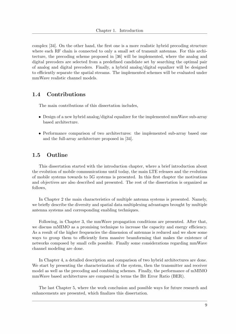
The first configuration is a SISO which is the simplest form of radio link. This transmitteroperates with one antenna as does the receiver and there is no diversity and no additionalprocessing required. Obviously the advantage of SISO is the simplicity despite offering noprotection against interference and fading and these events will have impact in the system.An example is shown in figure 2.1.
Figure 2.2: SIMO configuration
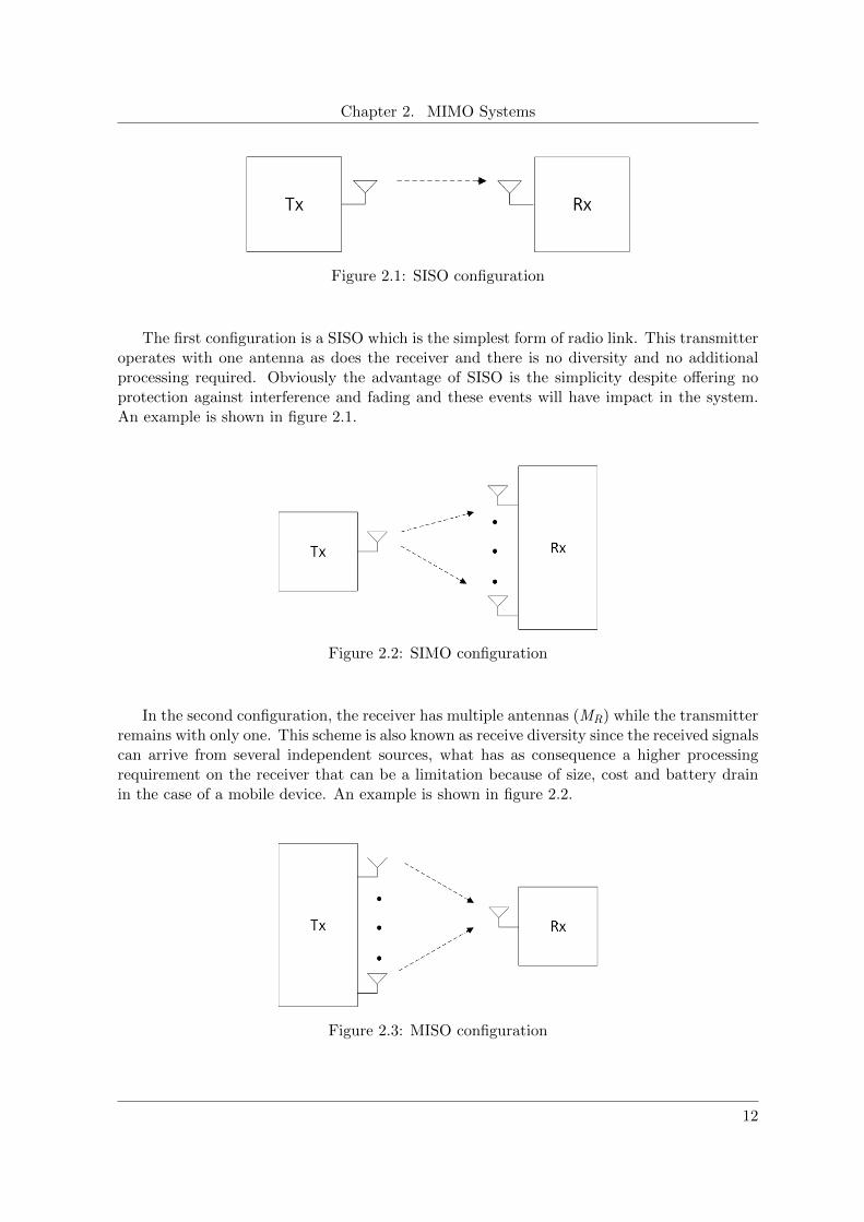
In the second configuration, the receiver has multiple antennas (MR) while the transmitterremains with only one. This scheme is also known as receive diversity since the received signalscan arrive from several independent sources, what has as consequence a higher processingrequirement on the receiver that can be a limitation because of size, cost and battery drainin the case of a mobile device. An example is shown in figure 2.2.
Figure 2.3: MISO configuration
12
Chapter 2. MIMO Systems
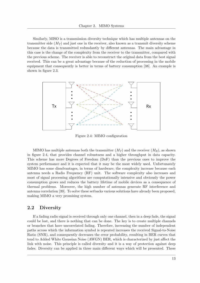
Similarly, MISO is a transmission diversity technique which has multiple antennas on thetransmitter side (MT) and just one in the receiver, also known as a transmit diversity schemebecause the data is transmitted redundantly by different antennas. The main advantage inthis case is the change of the complexity from the receiver to the transmitter, compared withthe previous scheme. The receiver is able to reconstruct the original data from the best signalreceived. This can be a great advantage because of the reduction of processing in the mobileequipment that consequently is better in terms of battery consumption [38]. An example isshown in figure 2.3.
Figure 2.4: MIMO configuration
MIMO has multiple antennas both the transmitter (MT) and the receiver (MR), as shownin figure 2.4, that provides channel robustness and a higher throughput in data capacity.This scheme has more Degrees of Freedom (DoF) than the previous ones to improve thesystem performance and it is expected that it may be the most widely used. UnfortunatelyMIMO has some disadvantages, in terms of hardware; the complexity increase because eachantenna needs a Radio Frequency (RF) unit. The software complexity also increases andmost of signal processing algorithms are computationally intensive and obviously the powerconsumption grows and reduces the battery lifetime of mobile devices as a consequence ofthermal problems. Moreover, the high number of antennas generate RF interference andantenna correlation [39]. To solve these setbacks various solutions have already been proposed,making MIMO a very promising system.
2.2 Diversity
If a fading radio signal is received through only one channel, then in a deep fade, the signalcould be lost, and there is nothing that can be done. The key is to create multiple channelsor branches that have uncorrelated fading. Therefore, increasing the number of independentpaths across which the information symbol is repeated increases the received Signal-to-NoiseRatio (SNR), and consequently decreases the error probability, resulting in BER curves thattend to Added White Gaussian Noise (AWGN) BER, which is characterized by just affect thelink with noise. This principle is called diversity and it is a way of protection against deepfades. Diversity can be applied in three main different ways which will be presented. These
13
Chapter 2. MIMO Systems
methods, therefore, reduce the probability that all the replicas are simultaneously affected bysevere attenuation and noise [40] [41].
Commonly used diversity techniques are:
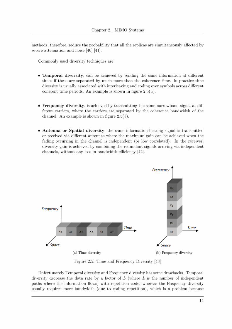
• Temporal diversity, can be achieved by sending the same information at differenttimes if these are separated by much more than the coherence time. In practice timediversity is usually associated with interleaving and coding over symbols across differentcoherent time periods. An example is shown in figure 2.5(a).
• Frequency diversity, is achieved by transmitting the same narrowband signal at dif-ferent carriers, where the carriers are separated by the coherence bandwidth of thechannel. An example is shown in figure 2.5(b).
• Antenna or Spatial diversity, the same information-bearing signal is transmittedor received via different antennas where the maximum gain can be achieved when thefading occurring in the channel is independent (or low correlated). In the receiver,diversity gain is achieved by combining the redundant signals arriving via independentchannels, without any loss in bandwidth efficiency [42].
(a) Time diversity (b) Frequency diversity
Figure 2.5: Time and Frequency Diversity [43]
Unfortunately Temporal diversity and Frequency diversity has some drawbacks. Temporaldiversity decrease the data rate by a factor of L (where L is the number of independentpaths where the information flows) with repetition code, whereas the Frequency diversityusually requires more bandwidth (due to coding repetition), which is a problem because
14
Chapter 2. MIMO Systems
this is a limited resource. However, the Spatial diversity is achieved without increasingthe bandwidth and the transmitted power, therefore there is a great interest for cellularcommunications [44] [45].
2.2.1 Receive Diversity
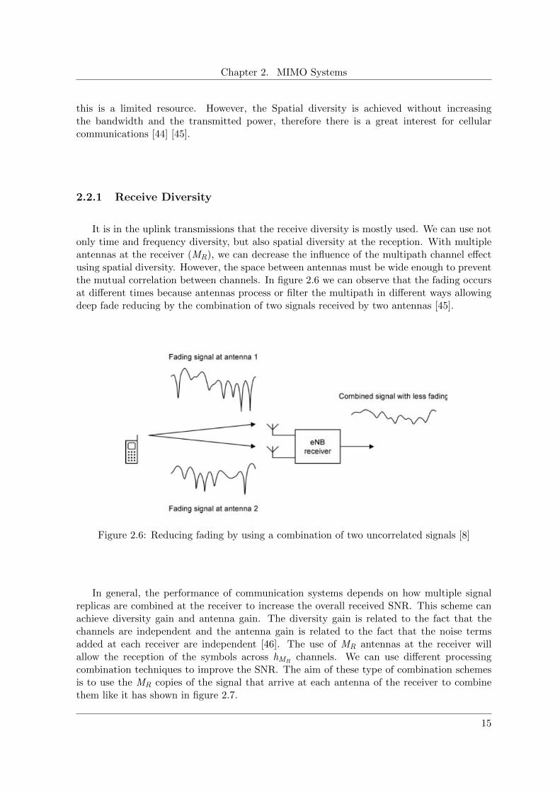
It is in the uplink transmissions that the receive diversity is mostly used. We can use notonly time and frequency diversity, but also spatial diversity at the reception. With multipleantennas at the receiver (MR), we can decrease the influence of the multipath channel effectusing spatial diversity. However, the space between antennas must be wide enough to preventthe mutual correlation between channels. In figure 2.6 we can observe that the fading occursat different times because antennas process or filter the multipath in different ways allowingdeep fade reducing by the combination of two signals received by two antennas [45].
Figure 2.6: Reducing fading by using a combination of two uncorrelated signals [8]
In general, the performance of communication systems depends on how multiple signalreplicas are combined at the receiver to increase the overall received SNR. This scheme canachieve diversity gain and antenna gain. The diversity gain is related to the fact that thechannels are independent and the antenna gain is related to the fact that the noise termsadded at each receiver are independent [46]. The use of MR antennas at the receiver willallow the reception of the symbols across hMR
channels. We can use different processingcombination techniques to improve the SNR. The aim of these type of combination schemesis to use the MR copies of the signal that arrive at each antenna of the receiver to combinethem like it has shown in figure 2.7.
15

Chapter 2. MIMO Systems
Figure 2.7: Spatial receive antenna diversity
The overall signal model for the received symbol will be the following
r1...
rMR
=
h1...
hMR
s+
n1...
nMR
(2.1)
and the estimated symbols are given by
s =[g1 . . . gMR
] r1...
rMR
(2.2)
s =[g1 . . . gMR
] h1...
hMR
s+[g1 . . . gMR
] n1...
nMR
(2.3)
According to the implementation complexity and the level of channel state informationrequired by the combining method, there are three main types of combining techniques,including Maximal Ratio Combining (MRC), Equal Gain Combining (EGC) and SelectionCombining (SC) [44] [46] [47].
16
Chapter 2. MIMO Systems
Maximal Ratio Combining
MRC is a linear combining. Various signal inputs are individually weighted and addedtogether to get an output signal. The weighting factor of each receiver antenna can be chosento be in proportion to its own signal voltage to noise power ratio. This scheme requires theknowledge of channel fading amplitude and signal phases. MRC is usually used when we wantto maximize the SNR in order to eliminate bad noise conditions at the reception. Hence, thegm coefficients computed, are equal to the conjugate transpose (.)H of the channel.
The optimal coefficients/weights for maximal-ratio combining in fading is
gm = h∗m m = 1, . . . ,MR (2.4)
Therefore, with accurate channel knowledge h at the receiver and using these weights thesignal at the output combiner is
s =
MR∑m=1
∣∣hm∣∣2s+
MR∑m=1
h∗mnm (2.5)
In this case the antenna gain Ag will be
Ag = MR (2.6)
Note that MRC maximizes SNR aligning the phases of all MR channel coefficients, andalso giving more weight to the best channels.
Equal Gain Combining
EGC is a suboptimal but simple linear combining method. This scheme just rotates thephases of the arrived signals at each antenna and then adds them together with equal gain.
The weights are given by
gm =h∗m|hm|
m = 1, . . . ,MR (2.7)
Using these weights the signal at the output combiner is
s =
MR∑m=1
∣∣hm∣∣s+
MR∑m=1
h∗m|hm|
nm (2.8)
In this case the antenna gain Ag will be smaller than the MRC case
Ag = 1 +π
4(MR − 1) (2.9)
If we compare 2.6 and 2.9 the performance of EGC is marginally inferior to maximumratio combining and the implementation complexity for EGC is less than the MRC.
17

Chapter 2. MIMO Systems
Selection Combining
A Selection Combining is a simple diversity combining method. This algorithm comparesthe instantaneous amplitude of each channel and chooses the antenna branch with the highestamplitude. Thus the received signals in the other antennas are ignored. In practice, the signalwith the highest sum of signal and noise power is usually used, since it is difficult to measurethe SNR. This may be implemented with a single receiver or with two receivers. A singlereceiver is clearly desirable from a cost, size and power consumption perspective, howeversome time must be made available for the antenna signals to be compared.
The selection algorithm comes to compare the instantaneous amplitude of each channeland choose the branch with the largest amplitude
|h|max = max[|h|1, . . . , |h|MR
](2.10)
The weight is given by
gmax = h∗max (2.11)
and the estimated symbols are
s = |hmax|2x+ h∗maxnmax (2.12)
Increasing MR yields diminishing returns in terms of antenna gain, therefore the biggestgain is obtained from MR = 1 to MR = 2, as shown by the following equation.
Ag =
MR∑m=1
1
m(2.13)
So we can see that in SC scheme Ag keeps growing with the receiver antenna number, butin a non-linear way, and lesser than in MRC case and EGC case.
2.2.2 Transmit Diversity
Transmit diversity uses two or more antennas at the transmitter side, and consequentlyreduces the fading. This case, may be a quite similar to the receive diversity, however itcan provide an opportunity for diversity without any need for additional receive antennasand the corresponding additional receiver chains at the terminal. Sending a signal from thetransmitter antennas to the receiver without any coding/precoding, the signal just will beadded together, which brings a risk of destructive interference, so it cannot achieve diversity.To obtain it, a precoder or a space-time/frequency coding can be used. There are two waysto obtain it: closed loop transmit diversity and open loop transmit diversity.
Closed loop
In the closed loop form, the transmitter sends copies of the signal over the different anten-nas, but before the transmission the signal is formated to improve the system performance bytaking into account the Channel State Information (CSI). At the receiver, the signals will bephased that avoid destructive interference. To ensure that the signals are received in phase,the phase shift is calculated by the receiver and fed back to the transmitter as a Precoding
18

Chapter 2. MIMO Systems
Matrix Indicator (PMI). A simple PMI might indicate if the signals must be transmittedwithout a phase shift, or instead, must be applied to a phase shift. In case of the first optionit leads to destructive interference, then the second will automatically work. This impliesthat the transmitter has previous acknowledge of the CSI [46]. The phase shifts occur in thefrequency domain and the PMI comes as a function of frequency.
In conclusion, if UEs are moving fast a delay is introduced in the feedback loop, the PMIwill change and cannot correspond to the best choice when it is received because the channelstate changes very quickly. This technique is suitable to relatively slowly moving mobiles.For users in fast movement the best choice could be the open loop techniques [8].
Open loop
In the open loop form, diversity is usually performed with space-time/frequency coding.Instead of a closed loop, the open loop techniques don’t require CSI, which offers robustnessagainst non-ideal conditions (like antenna correlation, channel estimation errors and Dopplereffects). Typically, there are mainly two types of space-time codes: trellis and block codes.The first ones usually outperform the block codes but at cost of higher complexity, and forthat reason their use in practical systems is limited. There are two types of block codes,Space-time Block Code (STBC) and Space-frequency Block Code (SFBC) [46] [48].
Figure 2.8: Alamouti technique for open loop transmit diversity
Figure 2.8 shows Alamouti’s block diagram for the open loop transmit diversity. Aftermodulating the information bits, using an M-ary modulation (e.g QAM), a block of two datasymbols s1 and s2 are coded in two antennas and in two frequency instants.
The matrix is
S =
[s1 −s∗2s2 s∗1
](2.14)
which means that in first time slot s1 and s2 are transmitted by antenna 1 and 2, respectively.In the second time slot −s∗2 and s∗1 are transmitted by antenna 1 and 2, respectively.
19

Chapter 2. MIMO Systems
If we perform the operation
S× SH =
[|s1|2 + |s2|2 0
0 |s1|2 + |s2|2]
(2.15)
we can show that S matrix is orthogonal. s1 and s2 are independent thus Alamouti code isan orthogonal code.
Figure 2.9: Alamouti receiver block diagram
The receiver side of Alamouti is represented in figure 2.9. Considering h =[h1 h2
]as the overall vector channel, h1 and h2 represents the channel coefficients of antenna 1 and2, respectively, n =
[n1 n2
]is the additive white Gaussian noise and the received signal
y in matrix notation is given by
y =1√2hS + n (2.16)
Each symbol is multiplied a factor 1/√
2 in order to normalize the power per symbol. Theprevious equation may be written as{
y1 = 1√2h1s1 − 1√
2h2s∗2 + n1
y2 = 1√2h1s2 + 1√
2h2s∗1 + n2
(2.17)
If the channels of two adjacent frequencies are highly correlated we can assume thathk,n ≈ hk,n+1, the estimated symbols after dividing are given by{
s1 = 1√2h∗1y1 + 1√
2h2y∗2 + n1
s2 = 1√2h1y∗1 + 1√
2h2y∗2 + n2
(2.18)
With channel knowledge available at the receiver, we will decode the symbols s, using thematched filter version of Heq, defined by
HHeq =
[h∗1 h2
h∗2 −h1
](2.19)
20

Chapter 2. MIMO Systems
consequently, the soft decision of data symbols are given by
s = hHeqy (2.20)
sn =1
2(h∗1h1 + h∗2h2)sn +
1√2h∗1nn +
1√2h2n
∗n+1 (2.21)
From 2.21, interference caused by n+ 1 data symbol is eliminated, thus SNR is
SNR =1
2
(|h1|2 + |h2|2)
σ2n
(2.22)
This presentation was made for a system with 2×1 antennas, where Alamouti scheme canachieve a diversity order of 2. Although it could be generalized for more than one antenna atthe receiver side. i.e for 2×MR system. In this case the diversity order that can be obtainedis 2MR with an antenna gain of MR. The above Alamouti STBC scheme is only availablefor 2 antennas at the transmitter. One possible solution of Alamouti coding in the case of 4antennas transmission is performing a time and space shift of Alamouti blocks using a STBC -Time Shift Transmit Diversity (STBC - TSTD) scheme as considered in the LTE, as is shownin Table 2.1.
t0 t1 t2 t3f0 s0 −s∗1 0 0f0 s1 s∗0 0 0f0 0 0 s2 −s∗3f0 0 0 s3 s∗2
Table 2.1: STBC - TSTD mapping [8]
2.3 Spatial Multiplexing
Spatial multiplexing has a different purpose from diversity processing. SIMO and MISOsystems provide diversity and antenna gains but no multiplexing gain. So if the transmitterand receiver both have multiple antennas, then we can set up multiple parallel data streamsbetween them. We can increase the data rate achieving also maximum capacity for the samebandwidth and without additional power. Another important aspect that must be verified toachieve high spatial multiplexing gain is low antenna correlation channel conditions. Thereforea high degree of difference between the channels is needed to perform the separation of multiplelayers without interference. In a system with MT transmit and MR receive antennas, oftenknown as an MT ×MR spatial multiplexing system, the peak data rate is proportional tomin(MT ,MR) compared with the SISO system [8].
Another important thing is that we can combine diversity and multiplexing in the samemultiple antenna system, but it is impossible to achieve their full benefits. If we consider a2 x 2 system, to have full diversity each symbol must go through two independent channelsso diversity is two (d = 2) and the multiplexing gain is one (r = 1). Now, to have full
21

Chapter 2. MIMO Systems
multiplexing on the same system, each channel is used by only one data stream (r = 2) butthere is no repetition of the symbols, so the diversity is one (d = 1). In the diversity, the datarate is constant and the BER decreases as the SNR increases and, in multiplexing, BER isconstant while the data rate increases with SNR [48].
2.3.1 SU-MIMO Techniques for Spatial Multiplexing
Using optimal Singular Value Decomposition (SVD), we are able to estimate the capacityof each channel in order to select the best channel to adapt the transmission. This adaptationis done by performing a power allocation according the singular values computed using SVD.We also obtain the optimum signal precoding to perform at the transmitter, and the neces-sary information for ideal equalization at the receiver. Denoting that CSI must be availableat both transmitter and receiver. However, sometimes just the receiver has a precise chan-nel information and in these cases the solution to decode the signal is just based on someequalization scheme performed at the receiver [40] [12].
Channel known at the transmitter
In the diagram of figure 2.10 it is represented the way of processing two spacial streams(green and orange), with spatial multiplexing.
Figure 2.10: Spatial multiplexing in a MIMO System
Let's analyze in detail the whole process to achieve spatial multiplexing. Inside the trans-mitter data symbols in the different antennas are precoded. The precoders are computedbased on the channel information that should be fed back from UE to the BS, consideringFDD mode, or estimated in the uplink if the TDD mode is assumed (channel reciprocity) [15].
Assuming that H =
h11 . . . h1,j
... hi,j...
hi,1 . . . hi,j
i = 1,. . . , MR; j = 1,. . . ,MT is the channel ma-
trix, x =[x1 . . . xMT
]Tis the vector of the transmitted signal, n =
[n1 . . . nMT
]T22

Chapter 2. MIMO Systems
is the noise vector and y =[y1 . . . yMR
]Tdefined by
y = Hx + n (2.23)
The transmitted signal x is defined as
x = Ws (2.24)
where W is the precoder matrix and s = [s1, . . . , sr]T is the data stream transmitted over the
MT antennas and r = min(MR,MT ).
Another way to describe the channel matrix is using the SVD. Channel H is now writtenas
H=UDVT (2.25)
where U and V are unitary with the size MR × r and MT × r respectively, r = rank(H) ≤min(MR, MT). D is the diagonal matrix composed by non-negative real numbers, defined by
D =
λ1 0 0
0. . . 0
0 0 λr
. (2.26)
The precoding matrix W is defined by
W=VP12 (2.27)
where the size is MT × r, and P is a square diagonal power allocation matrix of size r × rdefined by
p =
p1 0 0
0. . . 0
0 0 pr
. (2.28)
Setting the equalizer matrix as
G=UH (2.29)
Replacing in 2.23, the equations 2.24, 2.25 and 2.27, then
y=UDVTVP12 s + n (2.30)
The estimated data symbols in the receiver are obtained and given by
s = Gy = UHUDVTVP12 s + n (2.31)
s = DP12 s + n (2.32)
23

Chapter 2. MIMO Systems
The soft estimate of the rth data symbol is defined as
si = λi√pisi + ni i = 1, . . . , r (2.33)
The channel capacity via SVD decomposition is the following
C =r∑i=1
log2
(1 +
λ2i piσ2
)bits/s/Hz (2.34)
The selection of power that we will allocate in each channel is done in order to maximizethe system capacity. The amount of power put in each channel is done using the Water Fillingpower algorithm. Firstly, we select a limit called water level and then the amount of power is
distributed to the different channels. If the SNR(λ2iσ2
)of a channel is below the water level
the power allocated in this channel will be zero [49]. In figure 2.11 a specific realization ofthe Water Filling algorithm is presented.
Figure 2.11: Water Filling power scheme
Like we have seen the channels have different levels and the power must be distributedaccording to the SNR of each channel. Obviously, more power is allocated to better channelsand a reduced amount of power in bad channels. One way to find the best power allocationto optimize the system is using the Lagrangian method.
The optimal power allocation is then given by,
pi =
(β − 1
SNRi
)=
(β − σ2
λ2i
)(2.35)
where i, β and σ2 are respectively, the channel index, the water level value and the noisepower.
24
Chapter 2. MIMO Systems
Channel known only at the receiver
Like it was said before sometimes just the receiver has a precise channel information andwe are not able to use the SVD channel decomposition. In this case any precoding is performedat the transmitter side and the solution is just based in an equalization scheme performed atthe receiver. We can use linear equalizers, like Zero-Forcing (ZF) and Minimum Mean SquareError (MMSE), or non-linear equalizers like Successive Interference Cancellation (SIC) orParallel Interference Cancellation (PIC) applied together with linear equalizers [50] [51] [52].SIC and PIC establish a good compromise between performance and complexity improvingthe performance of linear equalizers ZF and MMSE.
Note, the signal model that will be considered is the same that was used in the previouslysubsection.
• ZF Equalizer
The aim of this technique is to design an equalizer vector for each data symbol toremove the interference using at least the same number of antennas at the receiver andtransmitter (MR ≥MT ).
The coefficients of this equalizer are given by
GZF =(HHH
)−1HH (2.36)
Despite of full symbol separation ZF amplifies the noise term which can be a problemin channels in deep fading.
• MMSE Equalizer
Instead of the use of ZF, we can improve the SNR using MMSE equalization. Thislatter one can enhance the noise when the channels are in deep fading or the channelscoefficients are correlated. This equalizer can be considered a trade-off between noiseenhancement and interference removal. It does not enable to achieve full interferenceremoval but prevents noise amplification.
The coefficients are obtained by minimizing the mean square error between the trans-mitted signal and the equalized output signal. These coefficients are given by
GMMSE =(HHH + σ2IMt
)−1HH (2.37)
25
Chapter 2. MIMO Systems
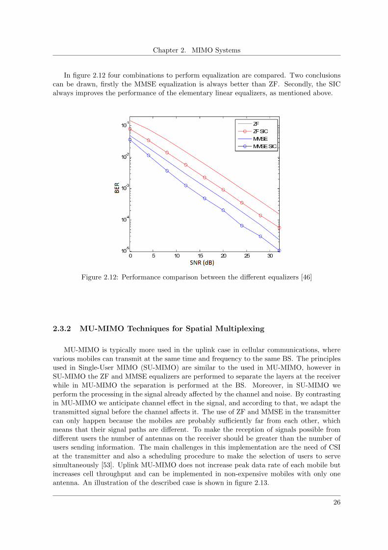
In figure 2.12 four combinations to perform equalization are compared. Two conclusionscan be drawn, firstly the MMSE equalization is always better than ZF. Secondly, the SICalways improves the performance of the elementary linear equalizers, as mentioned above.
Figure 2.12: Performance comparison between the different equalizers [46]
2.3.2 MU-MIMO Techniques for Spatial Multiplexing
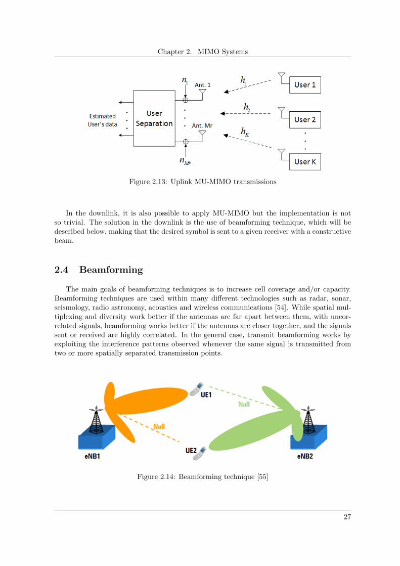
MU-MIMO is typically more used in the uplink case in cellular communications, wherevarious mobiles can transmit at the same time and frequency to the same BS. The principlesused in Single-User MIMO (SU-MIMO) are similar to the used in MU-MIMO, however inSU-MIMO the ZF and MMSE equalizers are performed to separate the layers at the receiverwhile in MU-MIMO the separation is performed at the BS. Moreover, in SU-MIMO weperform the processing in the signal already affected by the channel and noise. By contrastingin MU-MIMO we anticipate channel effect in the signal, and according to that, we adapt thetransmitted signal before the channel affects it. The use of ZF and MMSE in the transmittercan only happen because the mobiles are probably sufficiently far from each other, whichmeans that their signal paths are different. To make the reception of signals possible fromdifferent users the number of antennas on the receiver should be greater than the number ofusers sending information. The main challenges in this implementation are the need of CSIat the transmitter and also a scheduling procedure to make the selection of users to servesimultaneously [53]. Uplink MU-MIMO does not increase peak data rate of each mobile butincreases cell throughput and can be implemented in non-expensive mobiles with only oneantenna. An illustration of the described case is shown in figure 2.13.
26
Chapter 2. MIMO Systems
Figure 2.13: Uplink MU-MIMO transmissions
In the downlink, it is also possible to apply MU-MIMO but the implementation is notso trivial. The solution in the downlink is the use of beamforming technique, which will bedescribed below, making that the desired symbol is sent to a given receiver with a constructivebeam.
2.4 Beamforming
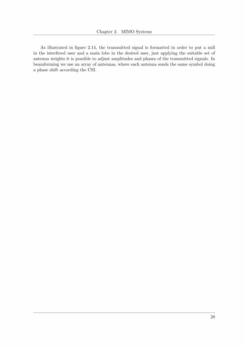
The main goals of beamforming techniques is to increase cell coverage and/or capacity.Beamforming techniques are used within many different technologies such as radar, sonar,seismology, radio astronomy, acoustics and wireless communications [54]. While spatial mul-tiplexing and diversity work better if the antennas are far apart between them, with uncor-related signals, beamforming works better if the antennas are closer together, and the signalssent or received are highly correlated. In the general case, transmit beamforming works byexploiting the interference patterns observed whenever the same signal is transmitted fromtwo or more spatially separated transmission points.
Figure 2.14: Beamforming technique [55]
27
Chapter 2. MIMO Systems
As illustrated in figure 2.14, the transmitted signal is formatted in order to put a nullin the interfered user and a main lobe in the desired user, just applying the suitable set ofantenna weights it is possible to adjust amplitudes and phases of the transmitted signals. Inbeamforming we use an array of antennas, where each antenna sends the same symbol doinga phase shift according the CSI.
28

Chapter 3
Millimeter Wave and MassiveMIMO Systems
The rapid increase of mobile data growth and the use of smartphones and other mobiledata devices such as netbooks and ebook readers are creating unprecedented challenges forwireless services [31]. The current 4G systems including LTE and WiMAX already use ad-vanced technologies in order to achieve spectral efficiencies close to the theoretical limits interms of bits per second. However LTE has been deploying and is reaching maturity, but itmay not be enough to support all requirements. 5G will need to be a paradigm shift thatincludes the use of much greater spectrum allocations at untapped mmWave frequency bands,highly directional beamforming antennas, longer battery life, lower outage probability, muchhigher bit rates in larger portions of the coverage area, lower infrastructure costs, and higheraggregate capacity for many simultaneous users [25].
So, the aim of this chapter is to discuss the main issues of mmWave, mMIMO, massivebeamforming and follows with the different proposals for antenna architectures at higherfrequencies. It also presents the fundamentals of channel modeling to be used in mmWavemMIMO systems and finishes with a briefly description of networks composed by small cells.
3.1 Millimeter Waves
Almost all mobile communication systems today use spectrum in the range of 300 MHz-3 GHz and in this section the reason why the wireless community should start looking atthe 3-300 GHz spectrum for mobile broadband applications. Almost all commercial radiocommunications among AM/FM radio, satellite communication, GPS and Wi-Fi containinga narrow band of RF spectrum between 300 MHz - 3 GHz, that is usually called ”sweetspot” due to its favorable propagation characteristics [56]. The global bandwidth shortagehas motivated the exploration of the underutilized mmWave frequency spectrum, being thisone of the key advantages, and represents a large amount of spectral bandwidth available forfuture broadband cellular communication networks [57].
29

Chapter 3. Millimeter Wave and Massive MIMO Systems
The current 4G systems including LTE and WiMAX already use advanced technologiessuch as Orthogonal Frequency Division Multiplexing (OFDM), MIMO, multi-user diversity,link adaptation, turbo code in order to achieve spectral efficiencies close to theoretical lim-its in terms of bits per second per Hertz per cell, however it is not the sufficient for futurenecessities. mmWave has been widely used for long range point-to-point communication formany years. However, the antennas and components used in these systems including PowerAmplifiers (PA), Low Noise Amplifiers (LNA), mixers, oscillators, synthesizers, modulators,demodulators are too big in size and consume too much power to be applicable in mobile com-munication [31] [56]. The steady advancement of semiconductor technologies (PAs, LNA’s,mixers, antennas, . . . ) implemented with GaAs, SiGe, InP, GaN, or CMOS processes hastriggered the possibility of utilizing mmWave frequencies for the next generation cellular datanetworks [58]. Recent studies suggest the combination of cost-effective CMOS technology,that can now operate well into the mmWave frequency bands, and high antenna gain at themobile and the BS, promoting the viability of mmWave wireless communications [25]
With increasing of RF carrier frequency, the mmWave wavelength is reduced and this isa way to exploit polarization [59–61] and spatial processing techniques [34, 62–66], such asmMIMO and adaptive beamforming, in large antenna arrays. The operators want to createsmaller cells, referred as pico and femto-cells, with ranges in the order of 10-200 m, in orderto increase frequency reuse. Smaller cells are attractive for the mmWave spectral band andthe large beamforming gains achievable with very large antenna arrays can conversely tomitigate the high mmWave path loss [26]. However backhaul become essential in this systemto promote flexibility and quality of communications.
Recently the portion above 3 GHz has been explored for short-range and fixed wirelesscommunications. For example Ultra-Wideband (UWB) in range of 3.1-10.6 GHz has beenproposed to enable high data rate connectivity in personal area networks. mmWave systemsfor point-to-point communication already exist and they can achieve multi gigabit data ratesat a distance of up to 1 km and in 2003 the Federal Communications Commission (FCC)announced that the 71-76 GHz, 81-86 GHz and 92-95 GHz frequency bands had becomeavailable to ultra-high-speed data communications including point-to-point wireless local areanetworks, mobile backhaul, and broadband [31]. This announcement became highly importantbecause the backbone networks of 5G will move from copper and fiber to mmWave wirelessconnections, allowing rapid deployment and cooperation between BSs.
Another important discussion is the propagation characteristics of mmWave. Since thepropagation loss in free-space depends on the frequency, higher frequencies are subject to ahigher signal attenuation than lower frequencies. Moreover, signals at lower frequencies canpenetrate easily through buildings, although the mmWave signals do not penetrate most solidmaterials very well. Rain and atmospheric absorption increase the propagation loss [25] [31].For all these reasons high frequencies, historically, were ruled out for cellular usage mainlydue to concerns regarding short-range and Non-Line-of-Sight (NLoS) coverage issues [28].
The figure 3.1 shows the rain attenuation and atmospheric absorption characteristics ofmmWave propagation. The propagation through the atmosphere depends primarily on at-mospheric oxygen, humidity, fog and rain as it can be seen in next Table 3.1.
30
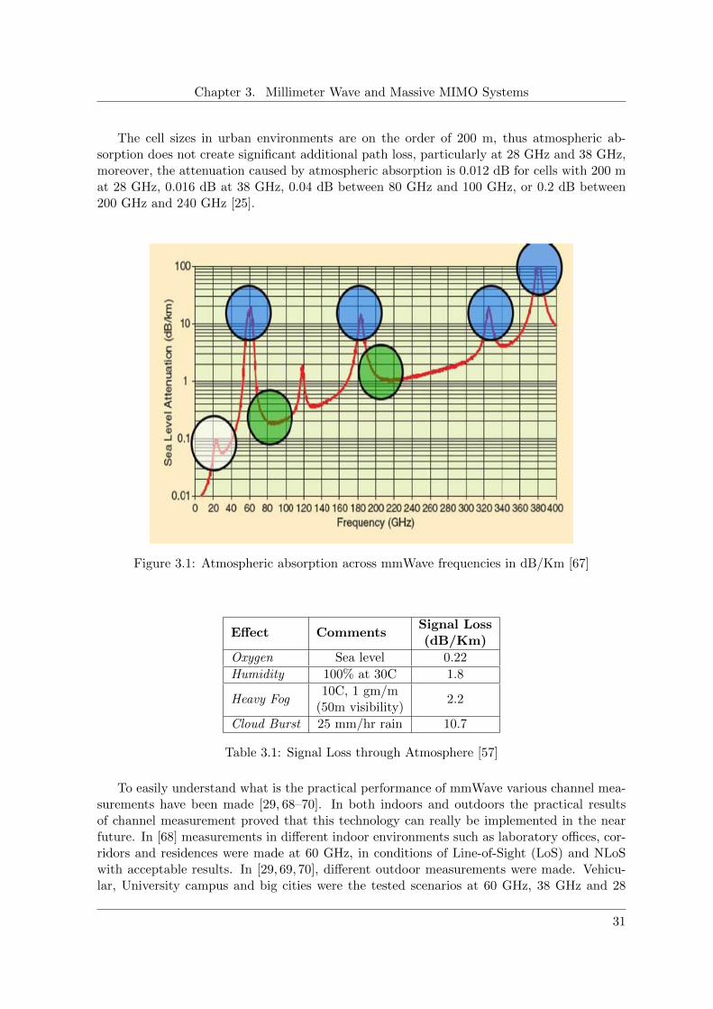
Chapter 3. Millimeter Wave and Massive MIMO Systems
The cell sizes in urban environments are on the order of 200 m, thus atmospheric ab-sorption does not create significant additional path loss, particularly at 28 GHz and 38 GHz,moreover, the attenuation caused by atmospheric absorption is 0.012 dB for cells with 200 mat 28 GHz, 0.016 dB at 38 GHz, 0.04 dB between 80 GHz and 100 GHz, or 0.2 dB between200 GHz and 240 GHz [25].
Figure 3.1: Atmospheric absorption across mmWave frequencies in dB/Km [67]
Effect CommentsSignal Loss(dB/Km)
Oxygen Sea level 0.22
Humidity 100% at 30C 1.8
Heavy Fog10C, 1 gm/m
(50m visibility)2.2
Cloud Burst 25 mm/hr rain 10.7
Table 3.1: Signal Loss through Atmosphere [57]
To easily understand what is the practical performance of mmWave various channel mea-surements have been made [29, 68–70]. In both indoors and outdoors the practical resultsof channel measurement proved that this technology can really be implemented in the nearfuture. In [68] measurements in different indoor environments such as laboratory offices, cor-ridors and residences were made at 60 GHz, in conditions of Line-of-Sight (LoS) and NLoSwith acceptable results. In [29, 69, 70], different outdoor measurements were made. Vehicu-lar, University campus and big cities were the tested scenarios at 60 GHz, 38 GHz and 28
31

Chapter 3. Millimeter Wave and Massive MIMO Systems
GHz, respectively. Sometimes difficulties were experienced and simple objects such as cars,windows or even people and trees have a major impact in mitigating the spread of mmWave.
3.2 Massive MIMO
MIMO technology has attracted much attention for wireless communications in the lastyears. The first approach was patented [71] in 1993, and the multiple transmit antennas wereplaced at one transmitter with the objective of improving the attainable link throughput.Basically, more antennas at the UEs and at the BSs create more DoF, which implies abetter performance in terms of data rate or link reliability without an additional increase inbandwidth or transmit power [27].
A particular case of MIMO is mMIMO systems where the basic premise behind is to reapall the benefits of conventional MIMO, but on a much greater scale. In some communitiesmMIMO defines any MIMO configuration beyond the highest MIMO mode in current LTE(at present 8x8), other communities refer mMIMO simply to large number of antennas at theBSs from tens to hundreds or also thousands [72].
mMIMO is presented as an enabler for the future digital society infrastructure that willconnect the Internet of people and Internet of Things with clouds and other network infras-tructure. This only can happen because it is expected that mMIMO will increase the capacity10 times or more and simultaneously improve the radiated energy efficiency in the order of100 times [73]. Moreover, this system with a large number of antennas, simultaneously servedozens of UEs without any penalty in user throughput and where the bandwidth efficiency isimproved and transmit power is reduced, as it is proved by measurements in [74]. The mul-tiplexing gains or diversity gains are improved due to the excessive DoF. The possibility totransmit simultaneously to several users and the flexibility to select what users are scheduledfor reception at any given point in time is another possibility. These arrays of antennas helpto focus energy with an extremely narrow beam reducing the inter-user interference even fur-ther by using, for example, ZF. However the number of terminals that can be simultaneouslyserved is limited, not by the number of antennas, but rather by our inability to acquire CSIfor an unlimited number of terminals [27]. New designs can be made extremely robust sothat the failure of one or a few of the antenna units would not appreciably affect the system,because if an individual antenna fails the system is prepared to be adaptable.
Many different configurations and deployment scenarios for the actual antenna arrays usedby a mMIMO system can be envisioned. The figure 3.2 illustrates several typical AntennaArray (AA), namely the linear AA, spherical AA, cylindrical AA, rectangular AA, and dis-tributed AA. The linear AA is related to traditional MIMO systems that can only adjustthe beam in the horizontal dimension [75]. This is an example of Two Dimensional (2D) thatis mostly assumed in theoretical analysis. In order to exploit the vertical dimension othertopologies may be considered. With these arrays it is possible to adjust both azimuth andelevation angles, and propagate signals in Three Dimensional (3D). The distributed antennaarray is used inside buildings and in outdoor cooperation [74].
32

Chapter 3. Millimeter Wave and Massive MIMO Systems
Figure 3.2: Antenna Array configurations mMIMO [74]
In mMIMO the BS needs to have good enough channel knowledge, on both the uplink andthe downlink. In case of the uplink this could be easy by having the terminals sending pilotsand based on which the BS estimates the channel responses to each of the terminals instead ofthe downlink that is more difficult. On the downlink, the BS sends out pilot waveforms thatthe terminals use to estimate the channel responses, and fed back to the BS. Unfortunately,for mMIMO systems this will not be feasible because the optimal downlink pilots shouldbe mutually orthogonal between the antennas, thus the amount of time-frequency resourcesneeded for downlink pilots scales with the number of antennas. Moreover, the number ofchannel responses that each terminal must estimate, again proportional to the number ofbase station antennas [75].
A main problem of conventional MIMO architectures in mMIMO implementations is thecomplexity of beamforming algorithms that make them impractical for commercial appli-cations, further to perform wideband digital beamforming, each signal from/to an antennaelement is usually divided into a number of narrowband signals and processed separately,which also adds a cost of digital signal processing. Therefore, a full digital signal implemen-tation is simply unrealistic, because the excessive demand on real time signal processing forhigh antenna gains. However, some solutions are being proposed to overcome the issues ofsignal processing and will be discussed in section 3.4.
33
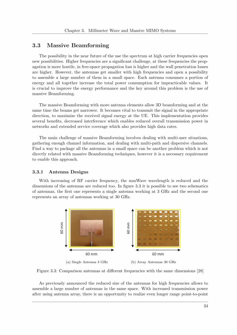
Chapter 3. Millimeter Wave and Massive MIMO Systems
3.3 Massive Beamforming
The possibility in the near future of the use the spectrum at high carrier frequencies opennew possibilities. Higher frequencies are a significant challenge, at these frequencies the prop-agation is more hostile, in free-space propagation loss is higher and the wall penetration lossesare higher. However, the antennas get smaller with high frequencies and open a possibilityto assemble a large number of them in a small space. Each antenna consumes a portion ofenergy and all together increase the total power consumption for impracticable values. Itis crucial to improve the energy performance and the key around this problem is the use ofmassive Beamforming.
The massive Beamforming with more antenna elements allow 3D beamforming and at thesame time the beams get narrower. It becomes vital to transmit the signal in the appropriatedirection, to maximize the received signal energy at the UE. This implementation providesseveral benefits, decreased interference which enables reduced overall transmission power innetworks and extended service coverage which also provides high data rates.
The main challenge of massive Beamforming involves dealing with multi-user situations,gathering enough channel information, and dealing with multi-path and dispersive channels.Find a way to package all the antennas in a small space can be another problem which is notdirectly related with massive Beamforming techniques, however it is a necessary requirementto enable this approach.
3.3.1 Antenna Designs
With increasing of RF carrier frequency, the mmWave wavelength is reduced and thedimensions of the antennas are reduced too. In figure 3.3 it is possible to see two schematicsof antennas, the first one represents a single antenna working at 3 GHz and the second onerepresents an array of antennas working at 30 GHz.
(a) Single Antenna 3 GHz (b) Array Antennas 30 GHz
Figure 3.3: Comparison antennas at different frequencies with the same dimensions [28]
As previously announced the reduced size of the antennas for high frequencies allows toassemble a large number of antennas in the same space. With increased transmission powerafter using antenna array, there is an opportunity to realize even longer range point-to-point
34

Chapter 3. Millimeter Wave and Massive MIMO Systems
LoS links which are the targeted applications, such as those providing wireless connectivitybetween aircrafts and/or between aircrafts and ground vehicles or control stations [76].
(a) Interleaved linear sub-arrays (b) Side-by-side linear sub-arrays
Figure 3.4: Hybrid Antenna Arrays [76]
To prevent grating lobes the antennas in the array must be placed closely together. Thisimplies that each antenna cannot be large compared to the wavelength, but also not toosmall and isotropic since some gain is needed to overcome the large path loss [26]. However,at 72 GHz the required element spacing is only about 2 mm and with current MonolithicMicrowave Integrated Circuits (MMIC) technology, the practical implementation of such adigital antenna array remains very difficult. In figure 3.4 two different ways are proposed toaccommodate a hybrid receive antenna, assembled like figure 3.3(b). These hybrid antennasare composed for 4 different sub-arrays of individual antennas and where each element in sub-array has its own RF chain [76]. The distance between adjacent elements in a sub-array isreferred to as the sub-array element spacing and the distance between corresponding elementsin adjacent sub-arrays is termed the sub-array spacing. In figure 3.4(a) the sub-array elementspacing is 2d and the sub-array spacing is d, whereas in figure 3.4(b) the sub-array elementspacing is d and the sub-array spacing is 4d.
Another issue of the use of conventional MIMO architecture in a mMIMO implementationis the necessity to replicate multiple transmit/receive chains, one per each antenna. Theanalog components, such as the LNA or PA and the down or up converter associated witheach antenna element, must be tightly packed behind the antenna element. For medium tohigh mmWave frequencies, antennas need to be located very close to their on-chip RF activecomponents. At lower frequencies, the antennas can be located off-chip, although still in closeproximity.
35

Chapter 3. Millimeter Wave and Massive MIMO Systems
(a) High Frequencies (b) Lower Frequencies (c) Block diagram of the RF
Figure 3.5: Antenna Front-End Integration [26]
The figure 3.5 shows an array of antennas with 128 elements. The solution of figure 3.5(a)can be implemented at very high frequencies. 4x4 RF chips (brown squares) are used, eachwith 8 antennas in the package (yellow squares) because the insertion loss to bring the signaloff-chip to an antenna would be too high. Instead, the solution of figure 3.5(b) will be usedfor lower frequencies. It is mounted nearby on a circuit board or on a different substrate,because at lower frequencies, the antennas are larger and not completely integrable in thechip package. In figure 3.5(c) a block diagram of the RF front-end with both TX and RXchannels integrated within the same chip is shown, and connected to 8 antennas in eitherconfiguration (a) or (b) [26].
Each antenna unit uses extremely low power, in the order of mW that enables the use ofrenewable energies, like wind and solar, to be the source of electric energy for the BS.
3.4 Architectures for mmWave mMIMO Systems
In this Section an overview of different mMIMO mmWave based architectures is done. InChapter 4 two of this architectures are evaluated and analyzed in detail. A major problemof conventional MIMO architecture in mMIMO implementations is the necessity to replicatemultiple transmit/receive RF chains. It is difficult to have a fully dedicated RF chain foreach antenna due the high cost and power consumption of some mixed signal components,like high-resolution analog-to-digital converters. This makes the conventional architectureused in current cellular systems, where precoding and combining are performed entirely inthe digital baseband absolutely impracticable.
To contribute for the developments new types of hybrid structures were proposed [32,33].The hybrid BF architectures use a much lower number of digital transceivers than the totalantenna number, allowing it to be more practical and improving the efficiency cost. Inthe hybrid based architectures, the transmitter and receiver processing are divided between
36

Chapter 3. Millimeter Wave and Massive MIMO Systems
the analog and digital domains. The approach proposed to reduce the transceiver numberis via analog BF [77], where each transceiver is connected with multiple active antennas.Additionally the signal is phased on each antenna and controlled by analog phase shiftersto obtain the maximal gain in the direction of the dominant channel paths. Thus, eachtransceiver generates one beam toward one user in analog BF. In relation to digital BF, overthe transceivers, this can then be utilized to achieve multiple data stream precoding on top ofanalog BF, to enhance the performance [32]. The main difficulty in hybrid BF design is mainlydue to the difficulty in CSI availability at BS transmitter side, because the mapping betweentransceivers and antennas makes channel estimation on both sides more complicated [78].
Different architectures have been designed, as the ones shown in figures 3.6, 3.7 and 3.8.Note that, N is the number of transceivers or RF chains and M represents the number ofactive antennas per transceiver.
3.4.1 Full-array architecture
Figure 3.6: Hybrid BF: Full-array architecture [78]
In the first hybrid BF architecture shown in figure 3.6, each transceiver is connected withall antennas, in such a way that the transmitter signal on each of the N digital transceiversflows trough NM RF paths (mixer, power amplifier, phase shifter, etc) and summed upbefore being connected with each antenna element. Further, analog BF is performed overNM RF paths per transceiver, and digital BF can then be performed over N transceivers [32].Obviously, the complexity of this architecture is rather high since the total number of RFpaths is N2M . However this architecture can achieve full BF gain.
37

Chapter 3. Millimeter Wave and Massive MIMO Systems
3.4.2 Sub-array architecture
Figure 3.7: Hybrid BF: Sub-array architecture [78]
The second hybrid BF architecture is shown in figure 3.7. Here, each of the N transceiversis connected to M antennas. Analog BF is performed over only M RF paths in eachtransceiver, and digital BF is performed over N transceivers [32]. This architecture is morepractical for BSs, where each transceiver is connected to a column of antennas. With activeantennas on each RF path, BF can be performed by applying different phases to each column.The beamforming gain obtained with this structure is usually lower, but the complexity isreduced [78].
3.4.3 1-bit ADC architecture
Figure 3.8: Hybrid BF: 1-bit ADC architecture [79]
38
Chapter 3. Millimeter Wave and Massive MIMO Systems
In the third hybrid BF architecture shown in figure 3.8, the use of low resolution Analogueto Digital Converter (ADC) is proposed. In mmWave systems, the sampling rate of the ADCsscales up with the larger bandwidth and, at present, commercially ADCs with high speed andhigh resolution are too costly and take up a great amount of power. A solution can be theuse of 1-bit ADC for each in-phase and quadrature baseband received signal, which reducespower consumption and cost. This architecture also simplifies the circuit complexity sinceautomatic gain control may not be required. Unfortunately, there are a few disadvantages;firstly more RF chains are required in receivers; secondly, the capacity that can be achievedis also limited [33].
3.5 Millimeter Wave MIMO channel
Transmission loss is accounted for principally by free space loss. A general misconceptionamong wireless engineers is that free-space propagation loss depends on frequency, thereforehigher frequencies propagate less well than lower frequencies [31].
Carrier wavelengths in mmWave are one order of magnitude smaller than those for exist-ing cellular and WiFi systems. As a result, the propagation and interference characteristics,limited by blockage of walls and furniture, are drastically different from our current expe-rienced in wireless network design. This fact results in a different propagation geometry.Omni-directional transmission is essentially infeasible because of the increased propagationloss at smaller wavelengths. On the other hand, highly directive transmission and receptionwith electronically steerable beams can be achieved using compact antenna arrays.
However, this high free-space pathloss, characteristic of mmWave, leads to limited spatialselectivity or scattering and the large tightly-packed antenna arrays, characteristic of mmWavetransceivers, lead to high levels of antenna correlation. A combination of tightly packed arraysin sparse scattering environments makes many of the statistical fading distributions used inconventional MIMO analysis inaccurate for mmWave channel modeling [34]. For all thesereasons new channel models for mmWave have been discussed for the next generation [29,30].
3.5.1 Types of channels
There are three typical channel models that have been used for evaluating performanceof wireless communications systems [74].
CBSM
Correlation-Based Stochastic Model (CBSM) has low complexity and it is mainly used forevaluating the theoretical performance of MIMO systems. However, it is somewhat simplisticand hence inaccurate for a realistic MIMO system. There are three different kinds of CBSM,i.e., the non-dispersive independent identically distributed (i.i.d.) Rayleigh fading model, the
39
Chapter 3. Millimeter Wave and Massive MIMO Systems
non-dispersive correlated channel model, and the dispersive multi-path channel model. Asummarized description of each is given below.
• Non-dispersive i.i.d. Rayleigh channel model: when this type of channel model isassumed no correlation existence between the transmit antennas and receive antennas.Consequently, the elements of the fast fading matrix are i.i.d. Gaussian variables.
• Non-dispersive correlated Rayleigh channel model: is a correlated channel modeland it is used to characterize the Doppler-induced received signal correlation. Thefast fading matrix of the correlated channel model is formed by the product of thecorrelation matrix and the standard complex-valued Gaussian matrix. The complex-valued Gaussian matrix describes the i.i.d. Rayleigh fading channel
• Dispersive multi-path channel model: this channel model can have different dis-tributions Angle of Arrival (AoA)s from different UEs. Each UE is constituted bymultiple independent paths, characterized by attenuation and AoA, from different di-rections. When UE are located at different angular positions, they can be separatedaccording to their AoA.
GBSM
Geometry-Based Stochastic Model (GBSM) model is capable of accurately describing therealistic channel properties, and hence is more suitable for mMIMO channels. However, itmust deal with an increased computational complexity, relatively to CBSM. According to themodeling of scattering propagation environments, the GBSM can be classified into single-ring,twin-ring and elliptical models. In mMIMO at higher frequencies elliptical model is the largestused and can be divided into 2D and 3D channel models. When BS is equipped with AA theangle of elevation is fixed and the 2D channel model is adequate for accurately evaluatingthe performance. Instead, when BS is equipped with a cylindrical or rectangular AA (seefigure 3.2) the 3D channel model with an adjustable angle of elevation has to be considered.
PSM
Parametric Stochastic Model (PSM) has higher complexity than CBSM and lower accu-racy than GBSM which represent a trade-off between the two channel models described above.PSM describes the signals on the receivers as a superposition of waves. There are models forconventional MIMO too, such as Double Directional Channel Model (DDCM) and VirtualRay Model (VRM). Nevertheless, PSM is less studied in context of mMIMO requiring furtherresearch efforts, before it becomes a reality. PSM constitute a viable alternative, which arecapable of reducing the complexity when compared with GBSM.
40

Chapter 3. Millimeter Wave and Massive MIMO Systems
3.5.2 Millimeter Wave MIMO Channel model
In this subsection we describe the clustered mmWave channel model presented in [34].Considering a single-user mmWave system with NT transmit antennas and NR receive anten-nas with Ncl scattering clusters where each cluster contribute with Nray propagation pathsto the channel matrix, the discrete-time narrowband channel H can be written as
H = γ∑i,l
αilΛr(φril, θ
ril
)Λt(φtil, θ
til
)ar(φril, θ
ril
)at(φtil, θ
til
)∗, (3.1)
where γ is a normalization factor such that γ =√NTNR/NclNray. The αil is the complex
gain of the lth ray in the ith scattering cluster, whereas φril (θril) and φtil (θtil) are its azimuth(elevation) angles of arrival and departure, respectively. The transmit and receive antennaelement gain at the corresponding angles of departure and arrival are given by the functionsΛt(φtil, θ
til
)and Λr
(φril, θ
ril
). The vectors ar
(φril, θ
ril
)and at
(φtil, θ
til
)represent the normalized
receive and transmit array response vectors at an azimuth (elevation) angle of φril (θril) and φtil(θtil) respectively. Finally, the αil follow a complex Gaussian distribution, CN
(0, σ2
α,i
)where
the σ2α,i represents the average power of the ith cluster.
An array response vector depends on the array antenna type. For a Uniform LinearArray (ULA) on the y-axis, with Ny elements, the array response vector is given by
aULA(φ)
=1√Ny
[1, ej1kd sin(φ), ej2kd sin(φ), . . . , ej(Ny−1)kd sin(φ)
]T(3.2)
For a Uniform Planar Array (UPA) in the yz -plane with Ny and Nz elements on the yand z axis respectively, the array response vector is given by
aUPA(φ, θ)
=1√NyNZ
[1, . . . , ejkd
(m sin(φ) sin(θ)+n cos θ
), . . . , e
(jkd(Ny−1) sin(φ) sin(θ)+(Nz−1) cos θ
)]T(3.3)
Where for the equations 3.2 and 3.3 k = 2π/λ, d is the inter-element spacing, 0 ≤ m ≤ Ny
and 0 ≤ n ≤ Nz.
41

Chapter 3. Millimeter Wave and Massive MIMO Systems
3.6 Small Cell Networks
The combination of small cell geometries, as shown in figure 3.9, mmWave communicationsand arrays with a massive number of antennas will be essential to dramatically improvewireless access and throughput [26]. Wireless communication systems have been designedtoward high spectral efficiency (SE) to support the explosively growing traffics. Both SmallCell Network (SCN) and mMIMO have been recognized as promising ways to provide high SEand Energy Efficiency (EE), which actually are two extreme ways to use the spatial resources,e.g., frequency reuse and spatial multiplexing.
Figure 3.9: HetNet utilizing a mix of macro, pico, femto and relay BS [80]
In HetNets, small and low power BSs are overlaid within the macro network based on trafficand coverage area, representing a new paradigm for significantly expanding network capacity.This represents an attractive cost-effective solution to provide a uniform user experience [81].The frequency reuse is increased through the creation of smaller cells, referred to as micro-cells, pico-cells and femto-cells. mmWave signals do not penetrate brick and other materialseasily and which implies that mmWave cells may have to be located strictly in indoors andoutdoors scenarios. Path loss, that is another critical problem in mmWave, can actually bebeneficial in small-cell scenarios, because SCN limits inter-cell interference.
In traditional networks, the SE metric is considered to be the main performance indicatorwhich measures how efficiently the frequency resources are utilized regardless of the efficientpower consumption. On the other hand, EE is emerging as one of the key performanceindicators for the next generation (5G) wireless communications systems due the currentenergy cost payable by operators for running their access networks [82].
Recently many valuable works analyzing the trade-off between EE-SE in mMIMO andSCN [81, 83–85]. The EE of SCN was analyzed in [81], and shown that increasing the BSdensity will improve the EE only when the circuit power consumption is less than a certainthreshold. In [85] the relationship SE-EE was analyzed for mMIMO and it is demonstratedthat the slope of the EE-SE curve only depends of the circuit power and bandwidth when theSE approaches zero. When the SE approaches infinity the relation depends on the numberof data streams. However, it is in the [84] that the most interesting analysis was done. They
42

Chapter 3. Millimeter Wave and Massive MIMO Systems
made a comparison between mMIMO and SCN to understand which are the performance ofthese systems. The conclusions demonstrate that when the number of cells is large, SCNis always more energy efficient than mMIMO. Instead, when the number of cells is small,mMIMO achieves higher EE than SCN, when the circuit power consumptions of mMIMO aremuch lower than SCN.
3.6.1 Cell Types
The HetNets, like is shown in figure 3.9, are composed by some different types of basestations or cells. The main differences between them are the coverage area, the transmittedpower and their size. The existence of different cell types with different sizes and character-istics made a better deployment of the cellular systems possible. The smaller cells made thedevelopment and deployment of networks in the higher populated areas easier and cheaper.Sometimes, these cells are called green cells due the enhances in EE of the networks [82].
Macro-cells, micro-cells, pico-cells and femto-cells have the following main differences [86]:
• Macro-cells: is a conventional base station with 20 W of power and the range is about1 Km to 20 Km. Macro-cell in hierarchical structure takes care of roaming mobiles.
• Micro-cells: is a conventional base station with 1 W to 5 W of power and the range isabout 500 m to 2 Km. Micro-cells takes care of slow traffic (pedestrians and in-buildingsubscribers).
• Pico-cells: the pico-cells are a small version of base stations, ranging in size from alaptop computer suitcase. They are designed to serve a very small area like a part ofbuilding, a street corner, railway stations etc. These are used to extend coverage in aindoor area where outdoor signals do not reach well or add network capacity in areaswith very dense uses.
• Femto-cells: Femto-cells are also called home base stations and are typically designedfor the use in a home or a small business. The current designs typically support 2 to4 active mobile phones. The relatively reduced distance for the user leads to a higherreceived signal strength. This will result in an improvement in capacity through increasesignal strength and reduced interference. Deploying femto-cells will enable more efficientuses of precious power and frequency resources.
When a cellular network is properly designed it is expected that the capacity increasesas well as the coverage area in the cell-edges and consequently the user experience is better,which also severely contributed for the offloading of traffic from the macro-cells to the smallercells. With the use of small cells the latency times in the downlink and uplink communicationsbecomes lower, allowing fastest connections and also a better performance.
43

Chapter 3. Millimeter Wave and Massive MIMO Systems
The Table 3.2 summarizes the main characteristics of each type of cell.
Macro Micro Outdoor Pico Indoor Pico Femto
Keyapplication
Large coverageareas
Medium coverageareas
Fit-in orextension
Indoor publicareas
Indoor residentialareas
Sectors 3 3 1 1 1
Number ofusers per cell
>200 Up to 200 Up to 100 Up to 50 <10
Mobility High High High Low Low
Typical RFoutput power
10 W 4 W 1 W 500 mW 100 mW
Cost High Medium High Medium Low Very Low
Table 3.2: Characteristics of the different base stations [87]
44

Chapter 4
Architectures and ProcessingTechniques for mmWave mMIMOSystems
As previously stated, a major problem of conventional MIMO architecture in a mMIMOimplementation is the necessity to replicate multiple transmit/receive RF chains. It is difficultto have a full dedicated RF chain for each antenna due to the high cost and power consump-tion of some mixed signal components, like high-resolution analog-to-digital converters. Thismakes the conventional architecture used in current cellular systems, where precoding andcombining are performed entirely in the digital baseband absolutely impracticable. Moreover,the large number of antennas have an impact in complexity of signal processing functions likechannel estimation, precoding, combining and equalization.
In order to accommodate mmWave with large antenna arrays is necessary to overcome thedifficulties of signal processing, once some signal processing is done at the digital level andsome left for the analog domain. Recently, some beamforming and/or combining/equalizationschemes have been proposed for hybrid architectures [34,36,62,88]. In [34], a hybrid spatiallysparse precoding and combining approach was proposed for mmWave mMIMO systems. Thefull-array architecture of mmWave channels was exploited to formulate the single-user multi-stream precoding/combining scheme as a sparse reconstruction problem. In [36] was con-sidered a mmWave mMIMO system with the sub-array architecture for hybrid precodingscheme to achieve the near-optimal performance with low complexity. The authors in [62]proposed a simple precoding scheme, only based on the knowledge of partial channel infor-mation at both terminals, in the form of AoA and Angle of Departure (AoD). A joint designof transmit-receive mixed analog/digital beamformers that aims at maximizing the receivedaverage signal-to-noise-ratio SNR for SC systems, was proposed in [88].
In this Chapter we implement a hybrid sub-array based architecture for mmWave systems,which is denominated by Hybrid Architecture 2 (HA-2). The performance is compared againsta hybrid full-array based architecture denominated by Hybrid Architecture 1 (HA-1). TheHA-1 can approach close to optimal performance, but it involves very high computationalcomplexity. For the full array architecture each RF chain is connected to all BS transmitantennas, which makes the analog precoder/beamformer complex to be implemented in hard-
45

Chapter 4. Architectures and Processing Techniques for mmWave mMIMO Systems
ware. The HA-2 proposes a more realistic hybrid precoding architecture with low complexity,where each RF chain is connected to only a small set of transmit antennas. For the imple-mented HA-2, the hybrid precoder proposed in [36] is considered and at the receiver side, anew hybrid equalizer is designed to efficiently separate the spatial streams. The results haveshown that the full-array architecture HA-1 can achieve better performance than sub-arrayone (HA-2) in almost all scenarios, as expected. However, the sub-array architecture canobtain acceptable performances (in some scenarios outperforms HA-1), with a lower compu-tational complexity.
4.1 System Characterization
We consider a single-user mmWave system with Nt transmit antennas and Nr receiveantennas, where the transmitter sends Ns data streams to the receiver, per time-slot. Toenable multi-stream communication, the transmitter shown in figure 4.1 is equipped withNRFt transmit RF chains such that Ns ≤ NRF
t ≤ Nt. For the HA-2 each RF chain is onlyconnected to Nt / N
RFt antennas in the transmitter and Nr / N
RFr in the receiver, instead of
HA-1 where the transmitter/receiver are connected to all antennas.
For both, we consider a block fading channel, that remains constant during each blockbut varies independently between different blocks, with size T. The following characterizationis equally applied for both hybrid architectures. The received signal is given by
Y = HX + N (4.1)
where Y = [y1, . . . , yT ] ∈ CNr×T denotes the received signal matrix, X = [x1, . . . ,xT ] ∈CNt×T is the transmitted signal. N = [n1, . . . ,nT ] ∈ CNr×T is a zero mean Gaussian noisewith variance σ2
n. H ∈ CNr×Nt is the channel matrix, which follows the clustered sparsemmWave channel discussed in Chapter 3. We assume perfect timing and frequency syn-chronization. Moreover, we assume that the channel H is known perfectly at both sides,transmitter and receiver.
As mentioned before, channel H is a result from the sum of all contributions of Ncl clustersand each will contribute to Nray propagation paths for the channel matrix H, which may beexpressed as
H = ArΛAHt (4.2)
Λ is a diagonal matrix, with entries (i, l) that corresponds to the path gains of the lthray in the ith scattering cluster. The variables At = [at(θ
ti,l), . . . , at(θ
tNcl,Nray
)] and Ar =
[ar(θri,l), . . . , ar(θ
rNcl,Nray
)] are the matrix of array response vectors at the transmitter and
receiver, whereas θri,l and θti,l are respectively, the azimuth AoA and AoD.
46

Chapter 4. Architectures and Processing Techniques for mmWave mMIMO Systems
4.2 MmWave mMIMO Architecture 1
In Chapter 3 a general overview about this architecture was given. In this section wepresent in detail, the implemented one, including the design of beamformers/precoders andequalizer coefficients. The design of hybrid precoders are formulated as a sparsity constrainedmatrix reconstruction, that instead of directly maximizing mutual information, the near-optimal hybrid precoders can be found via an optimization of a sparse signal recovery withmultiple measurement vectors. The algorithm takes an optimal unconstrained precoder asinput and approximates it as linear combination of beam steering vectors. These vectorscan be applied at RF and combined digitally at baseband. It is also present the extensionof this sparse precoding approach to the receiver side. At the transmitter side a space-timeencoder structure is employed, before the digital and analog precoders to increase the inherentdiversity of the mmWave mMIMO system.
4.2.1 Transmitter Model Description
Figure 4.1: Transmitter block diagram for HA-1
The transmitter processing is decomposed into two parts, the digital and the analog, asshown in figure 4.1. These parts are modeled mathematically by Fa ∈ CNt×NRF
t matrix for theanalog part and Fd ∈ CNRF
t ×Ns matrix for the digital one. The analog part is implementedusing a matrix of analog phase shifters, due the hardware constraints, which force all elementsof matrix Fa to have equal norm (|Fa(i, l)|2 = N−1
t ). The transmit total power constraint isenforced by normalizing ||X||2F to NsT .
The analog part is followed by the digital part and no other hardware-related constraintsare placed on the baseband precoder, therefore the transmit signal is given by
X = FaFdC, (4.3)
where C = [c1, . . . , cT ] ∈ CNs×T denotes a codeword constructed using a STBC. The STBCconsidered can be mathematically described by
zt = Sft, (4.4)
ct = Πtzt, (4.5)
47
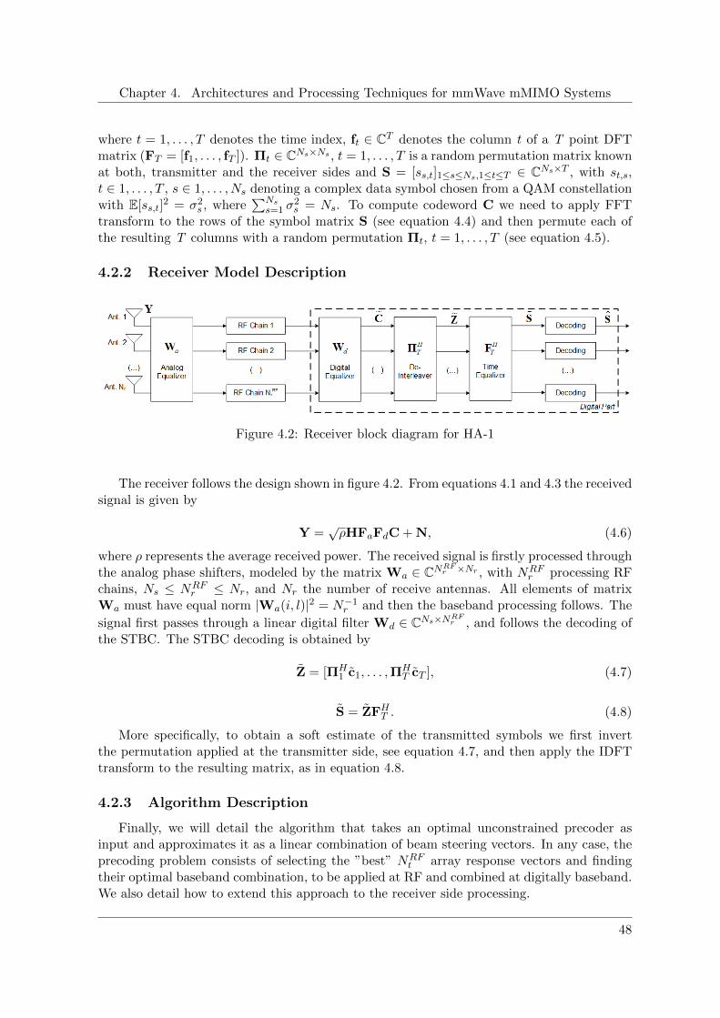
Chapter 4. Architectures and Processing Techniques for mmWave mMIMO Systems
where t = 1, . . . , T denotes the time index, ft ∈ CT denotes the column t of a T point DFTmatrix (FT = [f1, . . . , fT ]). Πt ∈ CNs×Ns , t = 1, . . . , T is a random permutation matrix knownat both, transmitter and the receiver sides and S = [ss,t]1≤s≤Ns,1≤t≤T ∈ CNs×T , with st,s,t ∈ 1, . . . , T , s ∈ 1, . . . , Ns denoting a complex data symbol chosen from a QAM constellationwith E[ss,t]
2 = σ2s , where
∑Nss=1 σ
2s = Ns. To compute codeword C we need to apply FFT
transform to the rows of the symbol matrix S (see equation 4.4) and then permute each ofthe resulting T columns with a random permutation Πt, t = 1, . . . , T (see equation 4.5).
4.2.2 Receiver Model Description
Figure 4.2: Receiver block diagram for HA-1
The receiver follows the design shown in figure 4.2. From equations 4.1 and 4.3 the receivedsignal is given by
Y =√ρHFaFdC + N, (4.6)
where ρ represents the average received power. The received signal is firstly processed throughthe analog phase shifters, modeled by the matrix Wa ∈ CNRF
r ×Nr , with NRFr processing RF
chains, Ns ≤ NRFr ≤ Nr, and Nr the number of receive antennas. All elements of matrix
Wa must have equal norm |Wa(i, l)|2 = N−1r and then the baseband processing follows. The
signal first passes through a linear digital filter Wd ∈ CNs×NRFr , and follows the decoding of
the STBC. The STBC decoding is obtained by
Z = [ΠH1 c1, . . . ,Π
HT cT ], (4.7)
S = ZFHT . (4.8)
More specifically, to obtain a soft estimate of the transmitted symbols we first invertthe permutation applied at the transmitter side, see equation 4.7, and then apply the IDFTtransform to the resulting matrix, as in equation 4.8.
4.2.3 Algorithm Description
Finally, we will detail the algorithm that takes an optimal unconstrained precoder asinput and approximates it as a linear combination of beam steering vectors. In any case, theprecoding problem consists of selecting the ”best” NRF
t array response vectors and findingtheir optimal baseband combination, to be applied at RF and combined at digitally baseband.We also detail how to extend this approach to the receiver side processing.
48

Chapter 4. Architectures and Processing Techniques for mmWave mMIMO Systems
Hybrid Analog/Digital Precoding
We seek to design mmWave precoders (Fa,Fd) that maximize the spectral efficiency. So,we start by examining the mutual information achieved by the hybrid precoders (Fa,Fd) toobtain the channel’s optimal unconstrained precoder Fopt. To do so, define the channel’sordered SVD to be,
H = UΣVH (4.9)
where V is an Nr × rank(H) unitary matrix and Σ is a rank(H)× rank(H) diagonal matrixof singular values arranged in decreasing order. Furthermore, defining the following twopartitions of the matrices Σ and V as
Σ =
[Σ1 00 Σ2
], V =
[V1 V2
], (4.10)
where Σ1 ∈ CNs×Ns and V1 ∈ CNt×Ns . We note that the optimal unconstrained unitaryprecoder for H is simply given by
Fopt = V1. (4.11)
With Fopt ∈ CNt×Ns , we defined the initial requirements to start building the algorithmpresented in Table 4.1, which takes an optimal unconstrained precoder as input and approx-imates it as linear combination of beam steering vectors.
Algorithm: Precoding step by step
Require: Fopt
1: Fa = Empty Matrix
2: Fres = Fopt
3: for i ≤ NRFt do
4: Ψ = AHt Fres
5: k = arg maxl=1,...,NclNray
(ΨΨH
)l,l
6: Fa =[Fa|A(k)
t
]7: Fd =
[FHa Fa
]−1FHa Fopt
8: Fres =Fopt−FaFd∣∣∣∣Fopt−FaFd
∣∣∣∣F
9: end for
10: Fd =√NS
Fd∣∣∣∣FaFd
∣∣∣∣F
return Fa, Fd
Table 4.1: Precoder algorithm for HA-1
49
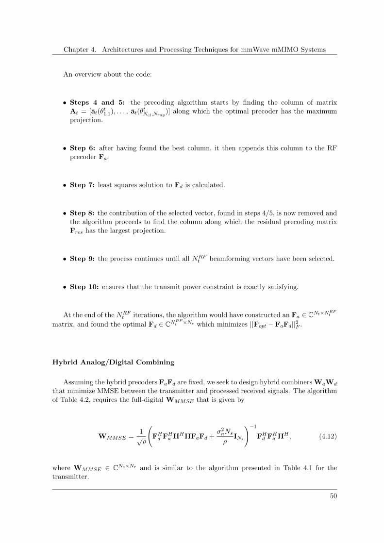
Chapter 4. Architectures and Processing Techniques for mmWave mMIMO Systems
An overview about the code:
• Steps 4 and 5: the precoding algorithm starts by finding the column of matrixAt = [at(θ
t1,1), . . . , at(θ
tNcl,Nray
)] along which the optimal precoder has the maximumprojection.
• Step 6: after having found the best column, it then appends this column to the RFprecoder Fa.
• Step 7: least squares solution to Fd is calculated.
• Step 8: the contribution of the selected vector, found in steps 4/5, is now removed andthe algorithm proceeds to find the column along which the residual precoding matrixFres has the largest projection.
• Step 9: the process continues until all NRFt beamforming vectors have been selected.
• Step 10: ensures that the transmit power constraint is exactly satisfying.
At the end of the NRFt iterations, the algorithm would have constructed an Fa ∈ CNt×NRF
t
matrix, and found the optimal Fd ∈ CNRFt ×Ns which minimizes ||Fopt − FaFd||2F .
Hybrid Analog/Digital Combining
Assuming the hybrid precoders FaFd are fixed, we seek to design hybrid combiners WaWd
that minimize MMSE between the transmitter and processed received signals. The algorithmof Table 4.2, requires the full-digital WMMSE that is given by
WMMSE =1√ρ
(FHd FH
a HHHFaFd +σ2nNs
ρINs
)−1
FHd FH
a HH , (4.12)
where WMMSE ∈ CNs×Nr and is similar to the algorithm presented in Table 4.1 for thetransmitter.
50

Chapter 4. Architectures and Processing Techniques for mmWave mMIMO Systems
Algorithm: Combining step by step
Require: WMMSE
1: Wa = Empty Matrix
2: Wres = WMMSE
3: for i ≤ NRFr do
4: Ψ = AHr E[yyH ]Wres
5: k = arg maxl=1,...,NclNray
(ΨΨH
)l,l
6: Wa =[Wa|A(k)
r
]7: Wd =
[WH
a E[yyH ]Wa
]−1WH
a E[yyH ]WMMSE
8: Wres = WMMSE−WaWd∣∣∣∣WMMSE−WaWd
∣∣∣∣F
9: end for
return Wa, Wd
Table 4.2: Combining algorithm for HA-1
In the algorithms design it was assumed perfect knowledge of the CSI, i.e. matrix H, whichmay be not feasible for practical systems. Moreover, in FDD based systems the receiver shouldfed back the matrix H to the transmitter in order to compute matrices Fa and Fd. Moredetails about these algorithms can be found in [34].
4.3 MmWave mMIMO Architecture 2
In this Section we present in detail the mmWave mMIMO HA-2 implemented with sub-array architecture (see figure 3.7), where each RF chain is connected to only an independentsubset from the total number of antennas [36]. As mentioned before, this sub-array architec-ture is less complexed than the previous one and for that reason it is a more realistic solutionfor practical implementation. Then, we also describe an iterative hybrid precoding schemebased on the SIC principle to achieve near-optimal performance with low complexity. Weconsider each antenna array one by one, which means that the precoding for each antennaarray is connected to a specific RF chain. For the first antenna array, we use the digitalprecoder to control the amplitude. After that, the analog precoder is applied to adjust thephase and then, the optimization problem for the first antenna array is solved with low com-plexity. The SIC approach is applied after the optimization problem for the first array. So,before solving the optimization problem for the second array of antennas we first eliminatethe contribution of the first array from the total achievable capacity. Generalizing, beforeoptimizing the capacity for an array we need to eliminate all contributions from the abovearrays. The only exception is for the first array, where obviously there is not any contributionto be removed. In figure 4.3 a diagram to easily understand the concept is shown.
51
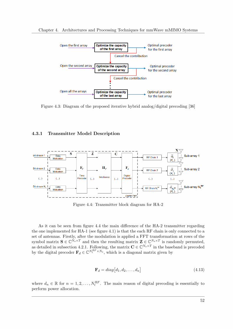
Chapter 4. Architectures and Processing Techniques for mmWave mMIMO Systems
Figure 4.3: Diagram of the proposed iterative hybrid analog/digital precoding [36]
4.3.1 Transmitter Model Description
Figure 4.4: Transmitter block diagram for HA-2
As it can be seen from figure 4.4 the main difference of the HA-2 transmitter regardingthe one implemented for HA-1 (see figure 4.1) is that the each RF chain is only connected to aset of antennas. Firstly, after the modulation is applied a FFT transformation at rows of thesymbol matrix S ∈ CNs×T and then the resulting matrix Z ∈ CNs×T is randomly permuted,as detailed in subsection 4.2.1. Following, the matrix C ∈ CNs×T in the baseband is precodedby the digital precoder Fd ∈ CNRF
t ×Ns , which is a diagonal matrix given by
Fd = diag[d1, d2, . . . , dn
](4.13)
where dn ∈ R for n = 1, 2, . . . , NRFt . The main reason of digital precoding is essentially to
perform power allocation.
52

Chapter 4. Architectures and Processing Techniques for mmWave mMIMO Systems
The digital part is followed by the analog part where the streams pass through thecorresponding RF chain, and the digital domain signal from each RF chain is deliveredto only Nt / N
RFt phase shifters to perform the analog precoding. The analog precoding
Fa ∈ CNt×NRFt , can be denoted by the analog weighting vector an ∈ C(Nt/NRF
t )×1, whose ele-ments have the same amplitude but different phases. The analog precoder matrix comprisingNRFt analog weighting vectors {am}m=1,...,NRF
tis given by
Fa =
a1 0 . . . 00 a2 0...
. . ....
0 0 . . . aNRFt
Nt×NRF
t
. (4.14)
After the analog precoding, each data stream is finally transmitted by a sub-array ofantennas.
4.3.2 Receiver Model Description
Figure 4.5: Receiver block diagram for HA-2
The receiver follows the design shown in figure 4.5, and the individual sub-arrays of receiveantennas (Nr / N
RFr per RF chain) is processed independently. The received signal can be
written as
Y = ρHFaFdC + N, (4.15)
where ρ is the average received power and N = [n1, . . . ,nT ] ∈ CNr×T is additive white
Gaussian noise with variance σ2n. For each time slot T, a vector yt =
[yt,1, yt,2, . . . , yt,Nr
]Tis extracted from the matrix Y and processed through the analog phase shifters, modeledby the matrix Wa ∈ CNRF
r ×Nr , then the baseband processing follows. The signal firstlypasses through a linear filter Wd ∈ CNs×NRF
r , which can again be generalized as Wd =diag
[d1, d2, . . . , dn
]where dn ∈ R for n = 1, 2, . . . , NRF
r , such as in transmitter side. However,before obtaining the soft estimation of the transmitted symbols, we first have to invert thepermutation applied at the transmitter side, see equation 4.7, and then apply the IDFTtransform, as in equation 4.8 to the resulting matrix S ∈ CNs×T .
53

Chapter 4. Architectures and Processing Techniques for mmWave mMIMO Systems
4.3.3 Algorithm Description
In this section, we present a low-complexity SIC-based hybrid precoding to achieve near-optimal performance, for the hybrid mmWave mMIMO based system discussed in the previoussection. According to the system model, the overall hybrid precoding matrix P can berepresented as P = FaFd = diag{a1, . . . , aNRF
t} × diag{d1, . . . , dNRF
t}.
There are three constraints for the P design. Firstly, P should be a block diagonal matrixsimilar to the form of Fa as shown in equation 4.14. We have P = diag{p1, . . . , pNRF
t},
where pn = dnan ∈ C(Nt/NRFt )×1 is the non-zero vector of the nth column pn of P. Secondly,
the non-zero elements of each column of P should have the same amplitude. Moreover, theamplitude of non-zero elements of the analog precoding matrix Fa is fixed to 1/
√Nt. The last
constraint, is related with the fact of the Frobenius norm of P should satisfy ||P||F ≤ NRFt
to meet the total transmit power constraint. However, these constraints are very difficult tobe solved.
So, based on special diagonal structure of hybrid precoding matrix P, we can observe thatthe precoding on each sub-array of antennas is independent. Therefore, we decompose thetotal achievable capacity into a series of sub-optimization problems. We start by designing thedigital-analog precoders and then we present the the analog-digital equalizer implemented.
Hybrid Analog/Digital Precoding
The aim is to design mmWave precoders (Fa,Fd) that maximize the performance foreach sub-array. To obtain this precoders we apply the SIC idea previously described, whichproceeds in steps and decompose the global optimization problem in several subproblems.Let us define the total achievable rate after m decompositions as
Tm = IN +ρ
σ2HP(1 : m)P(1 : m)HHH , (4.16)
where P(1 : m) denotes the first m columns of P and Tm ∈ CNr×Nr . Let us also describethe matrix G ∈ CNt×Nt
G = HHT−1m H. (4.17)
After each sub-optimization, we must find the remaining achievable rate Tm, and updatethe matrix G. Then, we define matrix Q of size M ×M as a sub-matrix of G by only keepingthe rows and columns of G for the sub-array of antennas that will be optimized. DenoteM = Nt/N
RFt as a number of antennas for each RF chain. Define the ordered SVD of the
Hermitian matrix Q as Q = UΣVH , where Σ is an M ×M diagonal matrix containing thesingular values of Q in a decreasing order, and V is an M ×M unitary matrix. We obtainv1 extracting the first column of V with size M × 1. The analog precoder for an individualsub-array of antennas is given by
am = ejangle(v1), (4.18)
where angle(v1) denotes the phase vector of v1.
54

Chapter 4. Architectures and Processing Techniques for mmWave mMIMO Systems
To sum up, the pseudo-code of the implemented hybrid analog/digital precoding schemeis described in Table 4.3
Algorithm: Precoding step by step
Require: H, Nt, NRFt
1: P = 0Nt×NRFt
2: M = Nt
NRFt
3: for 1 ≤ m ≤ NRFt
4: G = HHT−1m H
5: Q = G(M(m− 1
): Mm,M
(m− 1
): Mm
)6: v1 =The first right-singular vector of Q
7: am = ejangle(v1), bm =
0M(m−1)×1
am
0M(N−1)×1
8: dm =
Re[vH1 am
]M
9: pm = dmbm
10: end for
11: Fa =[b1,b2, . . . ,bNRF
t
]12: Fd = diag
(d1, d2, . . . , dNRF
t
)13: P =
[p1,p2, . . . ,pNRF
t
]return Fa, Fd, P
Table 4.3: Precoder algorithm for HA-2
Hybrid Analog/Digital Combining
We present in detail the algorithm implemented at the receiver side, i.e., the hybrid digital-analog equalizer. In the design of equalizer we assume a decoupled joint transmitter-receiveroptimization problem, i.e., we consider fixed precoders Fa and Fd in the equalizer design. Wealso assume perfectly channel knowledge, to find the near-optimal hybrid combiners Wa andWd. Firstly, it is necessary to define Heq ∈ CNr×Ns as
Heq = HFaFd (4.19)
and also rewriting the equation 4.16
Tm = IN +ρ
σ2HeqWopt(1 : m)Wopt(1 : m)HHH
eq (4.20)
where Wopt = WdWa is a matrix Ns ×Nr.
55

Chapter 4. Architectures and Processing Techniques for mmWave mMIMO Systems
After NRFr iterations, we use a ZF equalizer to efficiently remove the interference described
as
WZF =(HHo Ho
)−1Wopt, (4.21)
where Ho = Wopt ×Heq and WZF ∈ CNs×Nr . To sum up, the pseudo-code of the proposedhybrid analog/digital equalizer scheme is described in Table 4.4
Algorithm: Combining step by step
Require: H, Fa, Fd, Nr, NRFr
1: Wopt=0Nr×NRFr
2: M = Nr
NRFr
3: Heq = HFaFd
4: for 1 ≤ m ≤ NRFr
5: G = HHeqT
−1m Heq
6: Q = G(M(m− 1
): Mm,M
(m− 1
): Mm
)7: v1 =The first right-singular vector of Q
8: am = ejangle(v1), bm =
0M(m−1)×1
am
0M(N−1)×1
9: dm =
Re[vH1 am
]M
10: wm = dmbm
11: end for
12: Wa =[b1,b2, . . . ,bNRF
r
]13: Wd = diag
(d1, d2, . . . , dNRF
r
)14: Wopt =
[w1,w2, . . . ,wNRF
r
]Return: Wa, Wd, Wopt
Table 4.4: Combining algorithm for HA-2
4.4 Performance Results
This section presents a set of performance results for both implemented hybrid receiverarchitectures HA-1 and HA-2. It is considered a clustered channel model withNcl = 8 clusters,each with Nray = 10 rays, with Laplacian distributed azimuth angles of arrival and departure.The average power of all Ncl clusters is the same. The antenna element spacing is assumedto be half-wavelength. The channel remains constant during a block, with size T = 32, andtakes independent values between blocks. In the following, results for two different precoderswill be present: hybrid based precoders (Fa and Fd) and fixed hybrid random precoders thatare independent of the instantaneous channel realization, i.e. the phases of each phase shifter
56

Chapter 4. Architectures and Processing Techniques for mmWave mMIMO Systems
are set to a random value uniformly distributed between −π and π, and the digital part ofthe equalizer (Wd) is selected uniformly at random from the set of unitary matrices.
We will compare the performance of the presented schemes for three different scenarios,with the parameters described in Table 4.5.
TransmitRF chains
TransmitAntennas
ReceiveRF chains
ReceiveAntennas
Numberstreams
Scenario 1 4 64 4 16 4
Scenario 2 8 128 8 32 8
Scenario 3 16 256 16 64 16
Table 4.5: General parameters of the different scenarios
The Scenario 1 can be seen as the baseline scenario, and the other two scenarios are ascaling of the first. Note that the parameters of Scenario 2 are two times higher than theones of Scenario 1, and for Scenario 3 the parameters are two times and four times higherthan Scenario 2 and 1.
The metric performance considered is the average BER, which is presented as a functionof the Eb/N0, with Eb denoting the average bit energy and N0 denoting the one-sided noisepower spectral density. We consider σ2
1 = . . . ,= σ2Ns
= 1 and then the average Eb/N0 isidentical for all streams s ∈ 1, . . . , Ns.
Figure 4.6: Performance of the proposed hybrid equalizer as a function of time slots (T ) forHA-1 and Scenario 3
57

Chapter 4. Architectures and Processing Techniques for mmWave mMIMO Systems
Let us start the analysis of the implemented analog-digital based architectures by verifyingthe impact of the parameter T. In figure 4.6 are presented the BER results for Scenario 3and different values of the parameter T. These results were obtained for an Eb/N0 = 0 dBand Eb/N0 = 10dB, for the hybrid precoders of the HA-1. From figure 4.6 we verify that thedecay of the BER with T is fast until T ≈ 32 and for T > 32 the additional gains obtainedby increasing the value of variable T are marginal. Therefore, all the following results areobtained for T = 32.
4.4.1 Scenario 1
This scenario is the one that requires the smallest number of antennas and RF chainsinvolved in processing. We start by presenting the performance for both architectures HA-1and HA-2 using hybrid random precoders as described above. As it can be seen from figure 4.7HA-1 outperforms HA-2 as expected, since each RF chain is connected to all transmit antennasand therefore the diversity gain is higher (or in terms of capacity the achievable rate is higher).Taking into account the average BER at the target 10−3 the gap between both architecturesis close to 6 dB. Figure 4.8 shows the performance comparison between the same architecturesbut now using hybrid precoders presented in Sections 4.2.3 and 4.3.3. For this case the HA-1only outperforms the HA-2 for low SNR regime, for Eb/N0 larger than -15 dB the HA-2outperforms the HA-1. Therefore, using the hybrid precoders seems that in some cases theHA-2 outperforms HA-1 contrarily to the case of using random precoders.
Figure 4.7: Performance comparison of both architectures considering hybrid random pre-coders, for Scenario 1
58
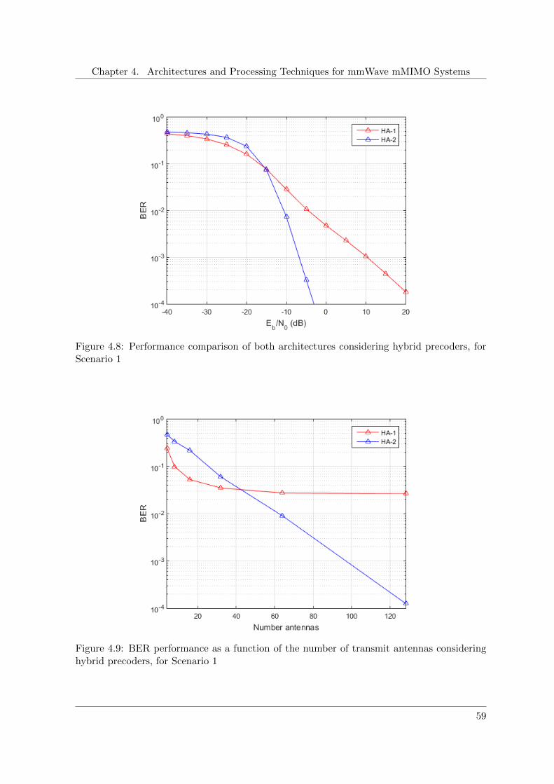
Chapter 4. Architectures and Processing Techniques for mmWave mMIMO Systems
Figure 4.8: Performance comparison of both architectures considering hybrid precoders, forScenario 1
Figure 4.9: BER performance as a function of the number of transmit antennas consideringhybrid precoders, for Scenario 1
59

Chapter 4. Architectures and Processing Techniques for mmWave mMIMO Systems
To try to understand the previous results obtained for hybrid precoders, we also evaluatethe performance impact with the number of transmit antennas for each architecture. Thesame values for the parameters described in Table 4.5 are considered, except the number oftransmit antennas that varies from 4 to 128. The results were obtained for a Eb/N0 = −10dB.From the results we can see that HA-1 outperforms HA-2 up to approximately 40 transmitantennas. After this point HA-2 clearly outperforms HA-1. For more than Nt = 40 theincreasing gain obtained for HA-1 is marginal, while for HA-2 the performance still improvewith the number of transmit antennas. This can be explained because both sides have 4RF chains and this means that for the first set of antennas (Nt=4) each RF chain has justone antenna for the HA-2, while HA-1 has RF chains connected for all antennas. When weincrease the number of antennas and keep the number of RF chains constant, we basicallyincrease the number of antennas in each sub-array that contribute to achieve the near-optimaloptimization.
4.4.2 Scenario 2
In Scenario 2 all parameters increased two times in relation to Scenario 1. Comparing theresults obtained for this scenario and for random and hybrid precoders (figures 4.10 and 4.11,respectively) with the ones obtained for Scenario 1 (figures 4.7 and 4.8), we can see that aperformance improvement of HA-1 and a performance degradation of HA-2. We can alsosee that for this scenario and considering random precoders HA-1 outperforms HA-2 for allEb/N0 range and for hybrid precoders there is a point (approximately -3 dB) from which HA-2outperforms HA-1. From figure 4.10 (random precoders), we can see that the gap betweenHA-1 and HA-2, at a target BER of 10−3, is 10.5 dB. The gap for the case where the hybridprecoders are used (figure 4.11) is 5.2 dB.
Figure 4.10: Performance comparison of both architectures considering hybrid random pre-coders, for Scenario 2
60

Chapter 4. Architectures and Processing Techniques for mmWave mMIMO Systems
Figure 4.11: Performance comparison of both architectures considering hybrid precoders, forScenario 2
Figure 4.12: BER performance as a function of the number of RF chains considering hybridrandom precoders, for Scenario 2
61

Chapter 4. Architectures and Processing Techniques for mmWave mMIMO Systems
In Scenario 1, we analyzed the influence in the number of antennas in both architectures.In this scenario and to try to understand the performance degradation of HA-2 when comparedto Scenario 1, we evaluated the BER performance as function of number of RFs chains asshown in figure 4.12. From this figure we can see that for HA-1 there is an optimal number ofRF chains that is approximately 13, less or larger this number the performance degrades. ForHA-2 we can see that the performance reduces as the number of RFs chain increases. Withthe increase of RFs chains HA-2 reduces the number of antennas for each sub-array and forthat reason the performance is reduced.
4.4.3 Scenario 3
In Scenario 3 the number of antennas and RF chains in transmitter and receiver sidesincreases two and four times in relation with Scenario 2 and 1, respectively. We also obtainedresults for random and hybrid precoders as in the Scenarios 1 and 2. From figures 4.13and 4.14 we can see that HA-1 outperforms HA-2 for both random and hybrid precoders andfor all Eb/N0 range. These results confirm the main conclusion of the previous scenarios. Infact HA-2 is highly sensitive to the number of RF chains since increasing it the number ofantennas processed at each RF chain is reduced and impacts a lot on the system performance.From figure 4.13, with random precoders, we can see that the gaps between HA-1 and HA-2,at a target BER of 10−3, is 15.8 dB. The gap for the case where de hybrid precoders are used(figure 4.14) is 13.8 dB.
Figure 4.13: Performance comparison of both architectures considering hybrid random pre-coders, for Scenario 3
62

Chapter 4. Architectures and Processing Techniques for mmWave mMIMO Systems
Figure 4.14: Performance comparison of both architectures considering hybrid precoders, forScenario 3
63

Chapter 4. Architectures and Processing Techniques for mmWave mMIMO Systems
64

Chapter 5
Conclusions and Future Work
The paradigm shift from 4G to 5G wireless system is driven by the expected huge growthin user bit rates and overall system throughput. The conventional wireless system is nearlyreaching maturity and will not be able to support the new requirements. MmWave communi-cations and mMIMO are seen as keys enabling elements for future 5G wireless communication.The adoption of mmWave transmission is mainly due to the huge bands available. Moreover,the small wavelength means small antennas, allowing transmitters and receivers to have alarge number of antenna elements. This results in many challenges to be solved related tohigh propagation free-space losses, absorption mainly due to obstacles, small diffraction ef-fects, different signal processing techniques, hardware complexity, cost, etc. Therefore, thereis many open problems that should be solved in the incoming years. In this dissertationwe contributed to understand part of these problems by implementing and comparing twodifferent hybrid architectures and processing techniques for mmWave mMIMO systems.
5.1 Conclusions
This dissertation started by presenting the evolution of mobile communications from thefirst to 4th generation. Then a briefly discussion about the forthcoming for 5th generation wasgiven. The progresses made over the years are remarkable, for mobile communications. Tobe truthful, mobile phones invaded our lives and they came to stay. Nowadays, these devicesare much more than voice communication equipment, they became our diaries, notebooks, inother words, they are our personal assistant in ”Anywhere, anything, anytime” in life and atwork. Just see, 1st generation voice transmissions were analog, while the 2nd had moved todigital. With the 3rd generation it became possible to access multimedia data services, whichchanged the way we look at mobile phones. Nowadays, it is easily to access for everythingalmost instantaneously with LTE. It is predictable that in the near future mobile phones willincrease their importance, serving us more and better services. Virtual Reality, Immerse orTactile Internet and Multi-person videoconferencing which are now hard to imagine, will bea common reality.
In the 2nd Chapter we have seen the ways of the use of multiple antenna systems in orderto achieve more throughput and coverage. Many of techniques studied are part of the currentsystems, exploiting diversity, spatial multiplexing and beamforming, usually on both sides ofthe system according to the requirements.
65

Chapter 5. Conclusions and Future Work
In the 3rd Chapter, the mmWave and mMIMO was described which is a promising ap-proach to achieve the multi Gigabit per second required by future wireless systems. Smallcells are also one of the key solutions to increase the capacity. Moreover, we identified relevanthybrid architectures for mmWave mMIMO systems, where the number of antennas is lowerthan the number of RF chains and the processing is done in two different domains, analog anddigital. This allows the use of a massive number of antennas to perform highly directionalbeams. It becomes vital to transmit the signal in the appropriate direction to maximize thereceived signal energy and overcome the issues of high path loss in mmWave.
The complexity remains one of the major difficulties to overcome in conventional systemsfor the next generation. So, in the 4th Chapter, two different hybrid architectures wereconsidered for mmWave mMIMO systems that can be part of the solution. The first one wasdesigned for a full-array architecture where each RF chain is connected to all antennas, thesecond one is a sub-array architecture where each RF chain is only connected to a small setof antennas.
We evaluated these architectures for different parameters/scenarios and the main conclu-sions are as follows:
• For a small number of RF chains the performance of HA-2 is better than HA-1 formedium to high Eb/N0 range. For higher numbers of RF chains HA-1 outperformsHA-2 for all Eb/N0 range.
• The HA-2 is high sensitive to the number of RF chains, since increasing this numberresults in degradation of the system performance.
• To mitigate the previously problem the number of antennas per RF chain should beincreased.
5.2 Future Work
Concerning the future work, we suggest the following improvements on the simulationplatform:
• We considered a single-user scenario, but use hundreds of antennas for one user cannot be a realistic scenario. Considering multi-user scenarios in future research, canpotentially increase the interest in lower complexity hybrid architectures.
• In this dissertation it was assumed perfect CSI at both sides. It would be useful toevaluate the implemented architectures under imperfect CSI.
• It would also be interesting to extend the processing from 2D scenario to 3D scenario,where the elevation angles of the AoA and AoD are taken into account.
• The optimization problem in both architectures was done in terms of capacity, it wouldbe interesting to formulate the optimization problem in terms of BER since the resultsare in function of BER.
66
Bibliography
[1] Vashu Kumar and Vipin Kumar. A new generation wireless mobile network-5g. Interna-tional Journal of Computer Applications, 70(20), 2013.
[2] The history of mobile phones from 1973 to 2008. [Available on-line at] http://www.knowyourmobile.com/nokia/nokia-3310/19848/
history-mobile-phones-1973-2008-handsets-made-it-all-happen. [Accessed]2016-05-28.
[3] M. L. Roberts, M. A. Temple, R. F. Mills, and R. A. Raines. Evolution of the air interfaceof cellular communications systems toward 4g realization. IEEE Communications SurveysTutorials, 8(1):2–23, First 2006.
[4] T. Emery. Cell phones: Hot/cold affair. The Cincinnati Enquirer, First 2004.
[5] Pankaj Sharma. Evolution of mobile wireless communication networks-1g to 5g as well asfuture prospective of next generation communication network. International Journal ofComputer Science and Mobile Computing, 2(8):47–53, 2013.
[6] 5G globalization or regionalization. [Available online at] https://siliconjoralemon.wordpress.com/2015/06/22/5g-globalization-or-regionalization/. [Accessed]2016-06-06.
[7] V. Pereira, T. Sousa, P. Mendes, and E. Monteiro. Evolution of mobile wireless: Fromvoice calls to ubiquitous multimedia group communications. 2nd International WorkingCOnference on Performance Modelling and Evaluation of Heterogenous Networks, Seventh2004.
[8] Christopher Cox. An introduction to LTE: LTE, LTE-advanced, SAE and 4G mobilecommunications. John Wiley & Sons, 2012.
[9] Global mobile subscribers and market share by technology. [Available online at] http://www.4gamericas.org/en/resources/statistics/statistics-global/. [Accessed]2016-05-31.
[10] Jorge Aido. MIMO Processing Techniques for Heterogeneous Cellular Systems. Master’sthesis, Universidade de Aveiro, the Portugal, 2015.
[11] Ajay R Mishra. Cellular technologies for emerging markets: 2G, 3G and beyond. JohnWiley & Sons, 2010.
67

Bibliography
[12] Farooq Khan. LTE for 4G Mobile Broadband: Air Interface Technologies and Perfor-mance. Cambridge University Press, New York, NY, USA, 1st edition, 2009.
[13] H. Holma and A. Toskala. LTE for UMTS - OFDMA and SC-FDMA Based RadioAccess. John Wiley Sons Ltd, New York, NY, USA, 2009.
[14] Summary of 3gpp standards releases for lte. [Available online at] http://www.3gpp.org/technologies/keywords-acronyms/98-lte. [Accessed] 2016-06-02.
[15] Alıcia Joao. Equalization and precoding techniques for future MC-CDMA systems. Mas-ter’s thesis, Universidade de Aveiro, the Portugal, 2014.
[16] G. A. Abed, M. Ismail, and K. Jumari. The evolution to 4g cellular systems: Architectureand key features of lte-advanced networks. International Journal of Computer Networksand Wireless Communications, 2(1):21–26, 2012.
[17] Ian F Akyildiz, David M Gutierrez-Estevez, and Elias Chavarria Reyes. The evolutionto 4g cellular systems: Lte-advanced. Physical Communication, 3(4):217–244, 2010.
[18] Hetnet/small cells. [Available online at] http://www.3gpp.org/hetnet. [Accessed] 2016-06-24.
[19] Highlights of 3gpp release 12. [Available online at] http://www.unwiredinsight.com/2014/highlights-of-3gpp-release-12. [Accessed] 2016-06-24.
[20] Evolution of lte in release 13. [Available online at] http://www.3gpp.org/news-events/3gpp-news/1628-rel13. [Accessed] 2016-06-25.
[21] C. Sharma. The Past, Present and Future of the Mobile Industry Evolution. MobileFutureForward, Seattle, USA, 2015.
[22] Peter Olanders. Network evolution towards 5g. Ericsson AB, 2015.
[23] D. Warren and C. Dewar. Understanding 5g: Perspectives on future technological ad-vancements in mobile. GSMA Intelligence, December 2014.
[24] W. Tong and Z. Peiying. 5G a technology vision. [Available online at] http://www1.huawei.com/en/about-huawei/publications/winwin-magazine/hw-329304.htm. [Ac-cessed] 2016-05-31.
[25] T. S. Rappaport, S. Sun, R. Mayzus, H. Zhao, Y. Azar, K. Wang, G. N. Wong, J. K.Schulz, M. Samimi, and F. Gutierrez. Millimeter wave mobile communications for 5gcellular: It will work! IEEE Access, 1:335–349, 2013.
[26] A. L. Swindlehurst, E. Ayanoglu, P. Heydari, and F. Capolino. Millimeter-wave massivemimo: the next wireless revolution? IEEE Communications Magazine, 52(9):56–62,September 2014.
[27] Fredrik Rusek, Daniel Persson, Buon Kiong Lau, Erik G Larsson, Thomas L Marzetta,Ove Edfors, and Fredrik Tufvesson. Scaling up mimo: Opportunities and challenges withvery large arrays. Signal Processing Magazine, IEEE, 30(1):40–60, 2013.
68

Bibliography
[28] W. Roh, J. Y. Seol, J. Park, B. Lee, J. Lee, Y. Kim, J. Cho, K. Cheun, and F. Aryanfar.Millimeter-wave beamforming as an enabling technology for 5g cellular communications:theoretical feasibility and prototype results. IEEE Communications Magazine, 52(2):106–113, February 2014.
[29] Y. Azar, G. N. Wong, K. Wang, R. Mayzus, J. K. Schulz, H. Zhao, F. Gutierrez,D. Hwang, and T. S. Rappaport. 28 ghz propagation measurements for outdoor cel-lular communications using steerable beam antennas in new york city. In 2013 IEEEInternational Conference on Communications (ICC), pages 5143–5147, June 2013.
[30] T. S. Rappaport, F. Gutierrez, E. Ben-Dor, J. N. Murdock, Y. Qiao, and J. I. Tamir.Broadband millimeter-wave propagation measurements and models using adaptive-beamantennas for outdoor urban cellular communications. IEEE Transactions on Antennasand Propagation, 61(4):1850–1859, April 2013.
[31] Z. Pi and F. Khan. An introduction to millimeter-wave mobile broadband systems. IEEECommunications Magazine, 49(6):101–107, June 2011.
[32] S. Han, C. l. I, Z. Xu, and C. Rowell. Large-scale antenna systems with hybrid analog anddigital beamforming for millimeter wave 5g. IEEE Communications Magazine, 53(1):186–194, January 2015.
[33] A. Alkhateeb, J. Mo, N. Gonzalez-Prelcic, and R. W. Heath. Mimo precoding andcombining solutions for millimeter-wave systems. IEEE Communications Magazine,52(12):122–131, December 2014.
[34] Omar El Ayach, Sridhar Rajagopal, Shadi Abu-Surra, Zhouyue Pi, and Robert W Heath.Spatially sparse precoding in millimeter wave mimo systems. Wireless Communications,IEEE Transactions on, 13(3):1499–1513, 2014.
[35] Xinyu Gao, Linglong Dai, Shuangfeng Han, Robert W Heath Jr, et al. Energy-efficienthybrid analog and digital precoding for mmwave mimo systems with large antenna arrays.arXiv preprint arXiv:1507.04592, 2015.
[36] Linglong Dai, Xinyu Gao, Jinguo Quan, Shuangfeng Han, and I Chih-Lin. Near-optimalhybrid analog and digital precoding for downlink mmwave massive mimo systems. InCommunications (ICC), 2015 IEEE International Conference on, pages 1334–1339. IEEE,2015.
[37] Ezio Biglieri, Robert Calderbank, Anthony Constantinides, Andrea Goldsmith, Aro-gyaswami Paulraj, and H Vincent Poor. MIMO wireless communications. Cambridgeuniversity press, 2007.
[38] Ian Poole. Mimo formats - siso, simo, miso, mu-mimo. [Available online at] http://www.radio-electronics.com/info/antennas/mimo/formats-siso-simo-miso-mimo.php.[Accessed] 2016-05-07.
[39] Michail Matthaiou. Mimo systems in wireless networks. Signal Processing Group, 2011.
[40] Stefania Sesia, Issam Toufik, and Matthew Baker. LTE-the UMTS long term evolution.Wiley Online Library, 2015.
69

Bibliography
[41] A. Sezgin. Space-Time Codes for MIMO systems Quasi-Orthogonal design and concate-nation. PhD thesis, Technische Universitt Berlin, Jun 2005.
[42] Manar Mohaisen, YuPeng Wang, and KyungHi Chang. Multiple antenna technologies.arXiv preprint arXiv:0909.3342, 2009.
[43] Alamouti space-time block coding. [Available online at] http://www.nutaq.com/blog/alamouti-space-time-block-coding. [Accessed] 2016-06-06.
[44] Yi Huang and Kevin Boyle. Antennas: from theory to practice. John Wiley & Sons,2008.
[45] Khaled Fazel and Stefan Kaiser. Multi-Carrier and Spread Spectrum Systems. WileyOnline Library, 1997.
[46] A. Silva and A. Gameiro. Multiple antenna systems lecture. Technical report, Universi-dade de Aveiro, 2016.
[47] Branka Vucetic and Jinhong Yuan. Space-time coding. John Wiley & Sons, 2003.
[48] Alain Sibille, Claude Oestges, and Alberto Zanella. MIMO: from theory to implementa-tion. Academic Press, 2010.
[49] Gustavo Anjos. Mimo processing techniques for 4g systems. Master’s thesis, Universidadede Aveiro, the Portugal, 2013.
[50] Mohinder Jankiraman. Space-time codes and MIMO systems. Artech House, 2004.
[51] David Tse and Pramod Viswanath. Fundamentals of wireless communication. Cambridgeuniversity press, 2005.
[52] Sergio Verdu. Multiuser detection. Cambridge university press, 1998.
[53] D. Gesbert, M. Kountouris, R. W. Jeath Fr., C. Chae, and T. Salzer. From singleuser to multiuser communications: Shifting the mimo paradigm. [Available online at]http://www.eurecom.fr/~gesbert/papers/TutorialMUMIMOv3.p. [Accessed] 2016-06-15.
[54] Agilent Technologies Application Note. Verify and visualize your td-lte beamformingsignals. 2012.
[55] Design and test challenges for 8x8 mimo devices for lte advanced. [Avail-able online at] https://www.wirelessdesignmag.com/article/2013/12/
design-and-test-challenges-8x8-mimo-devices-lte-advanced. [Accessed] 2016-06-13.
[56] F. Khan, Z. Pi, and S. Rajagopal. Millimeter-wave mobile broadband with large scalespatial processing for 5g mobile communication. In Communication, Control, and Com-puting (Allerton), 2012 50th Annual Allerton Conference on, pages 1517–1523, Oct 2012.
[57] Prasanna Adhikari. Understanding millimeter wave wireless communication. VP ofBusiness Development for Network Solutions, Loea Corporation, San Diego, 2008.
70

Bibliography
[58] W. Hong, Y. G. Kim, K. h. Baek, and Y. Lee. Design and testing of a millimeter-wavebeam-steering mesh-grid array for 5th generation (5g) mobile communication handsetdevices. In Radio Science Meeting (Joint with AP-S Symposium), 2014 USNC-URSI,pages 282–282, July 2014.
[59] Nicholas P Lawrence, Brian W-H Ng, Hedley J Hansen, and Derek Abbott. Analysis ofmillimeter-wave polarization diverse mimo capacity. In 2014 39th International Conferenceon Infrared, Millimeter, and Terahertz waves (IRMMW-THz), pages 1–2. IEEE, 2014.
[60] Qiang Xu, Houjun Sun, Jianyong Yin, and Xin Lv. A millimeter wave variable polar-ization monopulse frontend based on microstrip array antenna. In Microwave Technologyand Computational Electromagnetics, 2009. ICMTCE. International Conference on, pages264–267, Nov 2009.
[61] Qiao Xiaolin, Jin Tao, Qi Xiaohui, Zhang Min, Yuan Shuqing, and Zhang Qunxing. Anti-millimeter wave polarization agile active jamming. In Microwave and Millimeter WaveTechnology, 2007. ICMMT’07. International Conference on, pages 1–4. IEEE, 2007.
[62] A. Alkhateeb, O. El Ayach, G. Leus, and R. W. Heath. Hybrid precoding for millime-ter wave cellular systems with partial channel knowledge. In Information Theory andApplications Workshop (ITA), 2013, pages 1–5, Feb 2013.
[63] T. Obara, S. Suyama, J. Shen, and Y. Okumura. Joint fixed beamforming and eigenmodeprecoding for super high bit rate massive mimo systems using higher frequency bands. In2014 IEEE 25th Annual International Symposium on Personal, Indoor, and Mobile RadioCommunication (PIMRC), pages 607–611, Sept 2014.
[64] Andre BJ Kokkeler and Gerard JM Smit. Digitally assisted analog beamforming formillimeter-wave communication. In 2015 IEEE International Conference on Communi-cation Workshop (ICCW), pages 1065–1070. IEEE, 2015.
[65] Xinyu Gao, Linglong Dai, Chau Yuen, and Zhaocheng Wang. Turbo-like beamformingbased on tabu search algorithm for millimeter-wave massive mimo systems. 2015.
[66] Ahmed Alkhateeb, Geert Leus, and Robert W Heath. Limited feedback hybrid precodingfor multi-user millimeter wave systems. IEEE Transactions on Wireless Communications,14(11):6481–6494, 2015.
[67] T. S. Rappaport, J. N. Murdock, and F. Gutierrez. State of the art in 60-ghz integratedcircuits and systems for wireless communications. Proceedings of the IEEE, 99(8):1390–1436, Aug 2011.
[68] N. Moraitis and A. D. Panagopoulos. Millimeter wave channel measurements and mod-eling for indoor femtocell applications. In 2015 9th European Conference on Antennasand Propagation (EuCAP), pages 1–6, May 2015.
[69] E. Ben-Dor, T. S. Rappaport, Y. Qiao, and S. J. Lauffenburger. Millimeter-wave 60 ghzoutdoor and vehicle aoa propagation measurements using a broadband channel sounder.In Global Telecommunications Conference (GLOBECOM 2011), 2011 IEEE, pages 1–6,Dec 2011.
71
Bibliography
[70] J. N. Murdock, E. Ben-Dor, Y. Qiao, J. I. Tamir, and T. S. Rappaport. A 38 ghzcellular outage study for an urban outdoor campus environment. In 2012 IEEE WirelessCommunications and Networking Conference (WCNC), pages 3085–3090, April 2012.
[71] A.J. Paulraj and T. Kailath. Increasing capacity in wireless broadcast systems us-ing distributed transmission/directional reception (dtdr), September 6 1994. US Patent5,345,599.
[72] Berthold Panzner, Wolfgang Zirwas, Stefan Dierks, Mads Lauridsen, Preben Mogensen,Kari Pajukoski, and Deshan Miao. Deployment and implementation strategies for massivemimo in 5g. In Globecom Workshops (GC Wkshps), 2014, pages 346–351. IEEE, 2014.
[73] E. G. Larsson, O. Edfors, F. Tufvesson, and T. L. Marzetta. Massive mimo for nextgeneration wireless systems. IEEE Communications Magazine, 52(2):186–195, February2014.
[74] Kan Zheng, Long Zhao, Jie Mei, Bin Shao, Wei Xiang, and Lajos Hanzo. Survey oflarge-scale mimo systems. Communications Surveys & Tutorials, IEEE, 17(3):1738–1760,2015.
[75] Erik Larsson, Ove Edfors, Fredrik Tufvesson, and Thomas Marzetta. Massive mimo fornext generation wireless systems. Communications Magazine, IEEE, 52(2):186–195, 2014.
[76] X. Huang, Y. J. Guo, and J. D. Bunton. A hybrid adaptive antenna array. IEEETransactions on Wireless Communications, 9(5):1770–1779, May 2010.
[77] C. H. Doan, S. Emami, D. A. Sobel, A. M. Niknejad, and R. W. Brodersen. Designconsiderations for 60 ghz cmos radios. IEEE Communications Magazine, 42(12):132–140,Dec 2004.
[78] Shuangfeng Han, Chih Lin I, C. Rowell, Z. Xu, Sen Wang, and Zhengang Pan. Largescale antenna system with hybrid digital and analog beamforming structure. In 2014IEEE International Conference on Communications Workshops (ICC), pages 842–847,June 2014.
[79] R. Heath, A. Alkhateeb, J. Mo, and N. Gonzlez-prelcic. Millimeter wave mimo precod-ing/combining: Challenges and potential solutions, 2014.
[80] Qualcomm. Lte advanced: Heterogeneous networks. [Available online at] https://www.qualcomm.com/documents/lte-heterogeneous-networks. [Accessed] 2016-06-23.
[81] C. Li, J. Zhang, and K. B. Letaief. Throughput and energy efficiency analysis of smallcell networks with multi-antenna base stations. IEEE Transactions on Wireless Commu-nications, 13(5):2505–2517, May 2014.
[82] H. Pervaiz, L. Musavian, and Q. Ni. Energy and spectrum efficiency trade-off for greensmall cell networks. In 2015 IEEE International Conference on Communications (ICC),pages 5410–5415, June 2015.
[83] W. Liu, S. Han, and C. Yang. Energy efficiency comparison of massive mimo and smallcell network. In Signal and Information Processing (GlobalSIP), 2014 IEEE Global Con-ference on, pages 617–621, Dec 2014.
72
Bibliography
[84] Wenjia Liu, Shengqian Han, Chenyang Yang, and Chengjun Sun. Massive mimo or smallcell network: Who is more energy efficient? In Wireless Communications and NetworkingConference Workshops (WCNCW), 2013 IEEE, pages 24–29, April 2013.
[85] Z. Xu, S. Han, Z. Pan, and I. Chih-Lin. Ee-se relationship for large-scale antenna systems.In 2014 IEEE International Conference on Communications Workshops (ICC), pages 38–42, June 2014.
[86] RK Jain, Sumit Katiyar, and NK Agrawal. Hierarchical cellular structures in high-capacity cellular communication systems. arXiv preprint arXiv:1110.2627, 2011.
[87] D. Chang. Acceleraating global wimax adoption: The move to picocell and femtocell basesatations. [Available online at] http://www.embedded.com/print/4009436. [Accessed]2016-06-27.
[88] J. Nsenga, A. Bourdoux, and F. Horlin. Mixed analog/digital beamforming for 60 ghzmimo frequency selective channels. In Communications (ICC), 2010 IEEE InternationalConference on, pages 1–6, May 2010.
73

Bibliography
74