1

Comp 204: Computer Systems and Their Implementation

Lecture 12: Scheduling Algorithms cont’d

2

Today

•  Scheduling continued – Multilevel queues – Examples – Thread scheduling

Question •  A starvation-free job-scheduling policy guarantees that no job waits

indefinitely for service. Which of the following job-scheduling policies is starvation-free?

a)  Round-robin b)  Priority queuing c)  Shortest job first d)  Youngest job first e)  None of the above

3

Answer: a Round Robin – this gives all processes equal access to the processor. The other techniques each select some “types” of processes to others (e.g. short processes, high priority processes etc).

4

Question? •  Suppose that a scheduling algorithm

favours processes that have used the least CPU time in the recent past. Why will this algorithm favour I/O-bound programs and yet not permanently starve CPU-bound programs?

5

Answer

•  It will favour the I/O-bound programs because of their relatively short CPU burst times but, the CPU-bound programs will not starve because the I/O-bound programs will relinquish the CPU relatively often to do their I/O.

6

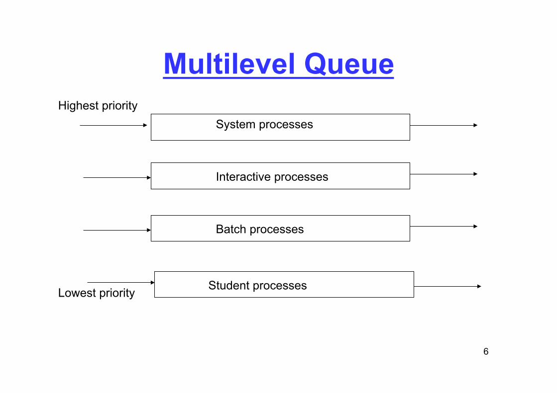
Multilevel Queue

System processes

Interactive processes

Student processes Lowest priority

Highest priority

Batch processes

7

Multilevel Queue •  Each queue has its own scheduling algorithm

–  e.g. queue of foreground processes using RR and queue of batch processes using FCFS

•  Scheduling must be done between the queues –  Fixed priority scheduling: serve all from one queue

then another •  Possibility of starvation

–  Time slice: each queue gets a certain amount of CPU time which it can schedule amongst its processes

•  e.g. 80% to foreground queue, 20% to background queue

8

Multilevel Feedback Queue •  A process can move between the various queues

–  Separates processes according to characteristics of their CPU bursts

–  I/O-bound processes stay in high-priority queues –  Compute-bound processes relegated to lower priority queues

•  Aging can be implemented to promote very long processes and hence prevent starvation

•  Parameters to be considered for a multilevel-feedback-queue scheduler: –  How many queues? –  Which algorithm is used for each queue? –  How to determine when to upgrade/demote a process to a

higher/lower priority? –  How to determine which queue a process will enter?

9

Example •  Three queues:

–  1) RR with time quantum of 4 milliseconds –  2) RR time quantum of 8 milliseconds –  3) FCFS

•  Scheduling –  A process at head of queue 1 gains the CPU for 4 milliseconds.

If it does not finish in 4 milliseconds, it is preempted and moved to tail of queue 2

–  When queue 1 is empty, the process at the head of queue 2 gets the CPU for 8 milliseconds. If it does not finish, it is preempted and moved to queue 3

–  When queues in 1 and 2 are empty processes in queue 3 are run FCFS

10

Multilevel Queues •  Advantages:

– Flexible implementation w.r.t. movement between queues

– Enables short CPU-bound jobs to be prioritised and therefore processed quickly

– Can be preemptive or non-preemptive

•  Disadvantages: – Queues require monitoring, which is a costly

activity

11

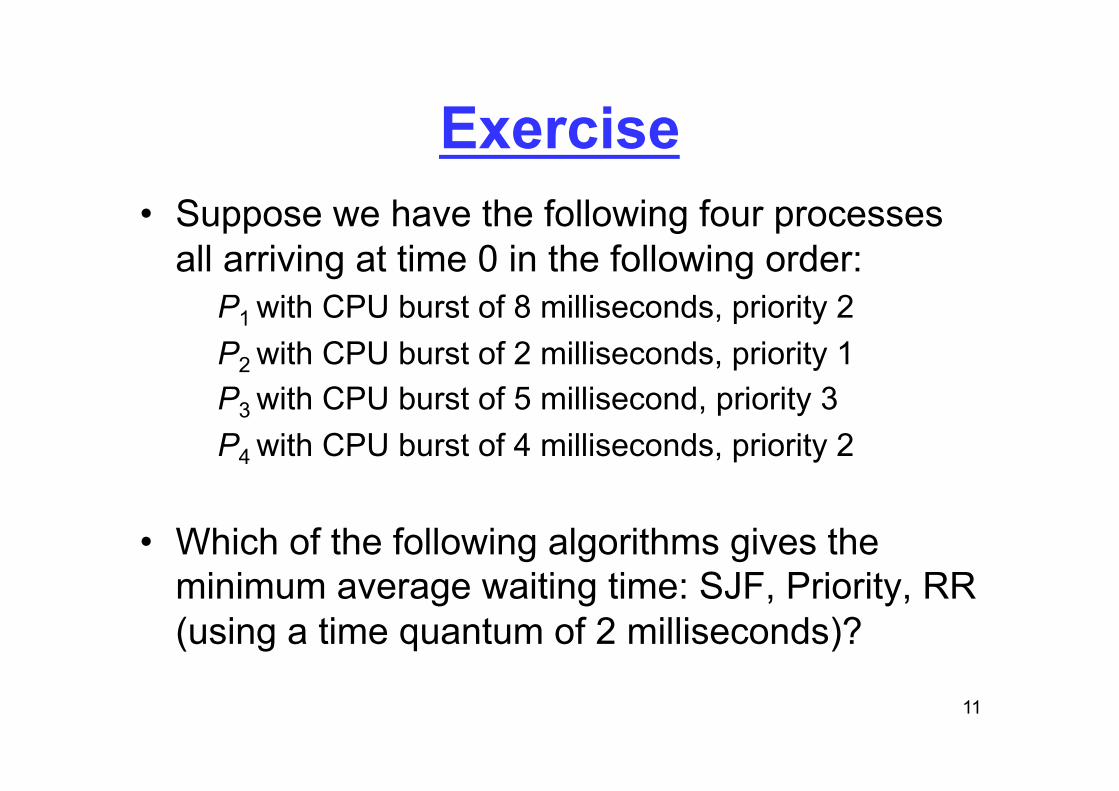
Exercise •  Suppose we have the following four processes

all arriving at time 0 in the following order: P1 with CPU burst of 8 milliseconds, priority 2 P2 with CPU burst of 2 milliseconds, priority 1 P3 with CPU burst of 5 millisecond, priority 3 P4 with CPU burst of 4 milliseconds, priority 2

•  Which of the following algorithms gives the minimum average waiting time: SJF, Priority, RR (using a time quantum of 2 milliseconds)?

12

Answer - SJF

•  SJF:

•  Average waiting time is (11 + 0 + 6 + 2)/4 = 4.75 milliseconds

0 2 6 11 19

P2 P4 P3 P1

P1 – CPU: 8 ms, priority 2 P2 – CPU: 2 ms, priority 1 P3 – CPU: 5 ms, priority 3 P4 – CPU: 4 ms, priority 2

13

Answer - Priority

•  Priority:

•  Average waiting time is (2 + 0 + 14 + 10)/4 = 6.5 milliseconds

0 2 10 14 19

P1 P3 P4 P2

P1 – CPU: 8 ms, priority 2 P2 – CPU: 2 ms, priority 1 P3 – CPU: 5 ms, priority 3 P4 – CPU: 4 ms, priority 2

14

Answer - RR

•  RR:

•  Average waiting time is ((17-6) + 2 + (16-4) + (12-2))/4 = 8.75 milliseconds

•  Thus, SJF gives the shortest average waiting time here

0 8 10 12 14 2 4 6 16 17 19

P1 P2 P3 P4 P1 P3 P4 P1 P1 P3

P1 – CPU: 8 ms, priority 2 P2 – CPU: 2 ms, priority 1 P3 – CPU: 5 ms, priority 3 P4 – CPU: 4 ms, priority 2

15

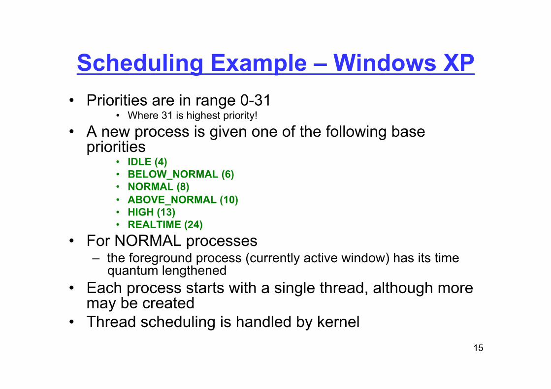
Scheduling Example – Windows XP •  Priorities are in range 0-31

•  Where 31 is highest priority!

•  A new process is given one of the following base priorities

•  IDLE (4) •  BELOW_NORMAL (6) •  NORMAL (8) •  ABOVE_NORMAL (10) •  HIGH (13) •  REALTIME (24)

•  For NORMAL processes –  the foreground process (currently active window) has its time

quantum lengthened •  Each process starts with a single thread, although more

may be created •  Thread scheduling is handled by kernel

16

Windows XP Threads •  Thread priorities divided into

–  Variable class (0-15) –  Real-time class (16-31)

•  Threads also have processor affinity –  CPUs may be real or virtual (hyper-threading)

•  Thread queue for each priority •  Dispatcher scans queues from highest to lowest to find

thread which is –  Ready to run –  Has affinity for CPU which is available

•  If no thread found, idle thread is executed

17

Windows XP Scheduling •  A thread can be pre-empted if a higher-priority real-time

thread becomes ready

•  If time-slice of normal class thread expires, its priority is lowered

•  When I/O or event wait completes for a normal class thread, priority is increased –  Increase is greater for slow I/O (e.g. keybd)

•  Thread associated with active window also gets priority increased

18

Linux Scheduling •  The Linux scheduler is a pre-emptive priority-based

algorithm –  Real-time tasks are distinguished from other tasks through the

use of priorities

•  The scheduler assigns longer time quanta to higher-priority tasks and shorter time quanta to lower-priority tasks

•  When the time-slice for a task expires, it is not eligible to be run again until all other tasks have used up their time quanta –  Priorities are dynamically recalculated when time-slice expires

19

Java Scheduling •  The JVM has a loosely-defined scheduling policy based

on priorities

•  It is possible for a lower-priority thread to continue to run even as a higher-priority thread becomes runnable, though some systems may support preemption

•  Using time-slicing, a thread runs until either: –  Its time quantum expires –  It blocks for I/O –  It exits its run() method

20

Java Thread Priorities

•  A thread is given a default priority, between 1 and 10, when created – The priority will be the same as the thread that

created it

•  This priority remains constant unless explicitly changed by the program – setPriority() method

21

End of Section •  Operating systems concepts:

–  communicating sequential processes; –  mutual exclusion, resource allocation, deadlock; –  process management and scheduling.

•  Concurrent programming in Java: –  Java threads; –  The Producer-Consumer problem.

•  Next section: Memory Management