commuting, congestion, and employment ... - mit economics

sal

to whichs actualeneratedat any

wagesh veryes andthat isoutput-

ersed.nitude

ed ons forants

ity,

Journal of Urban Economics 55 (2004) 417–438www.elsevier.com/locate/jue

Commuting, congestion, and employment disperin cities withmixed land use✩

William C. Wheaton

Department of Economics, Center for Real Estate, MIT, Cambridge, MA 02139, USA

Received 24 June 2003; revised 29 December 2003

Abstract

For centuries, cities have been modeled as having centered employment—scarce accessgenerates land rent. This paper first presents some new empirical evidence that in US citieemployment turns out to be almost as dispersed as residences. This range of urban forms is gwith analytic ease in a model that assumes land can have “mixed” rather than exclusive uselocation. The model has firms trading off a central-agglomeration force against the lowerthat accompany shorter commuting distances in peripheral locations. At one extreme, withigh agglomerative forces, employment is approximately centered, with long commute distanchigh congestion levels. At the other extreme, lower agglomerative forces lead to employmentcompletely dispersed, commute distances of zero and the absence of congestion. Maximizingminus-congestion never leads to a pattern of land mixing where employment is fully dispA market model, however, often does if the mix at each location is based on the relative magof the land rent offered from residential as opposed to commercial uses. 2004 Elsevier Inc. All rights reserved.

1. Introduction

Since the 19th century, the dominant view of urban land use has been basthe Ricardian rent, monocentric city model. In this model, transportation frictioncommuting or commerce generate a rent “gradient” between a city center and urbperiphery. As cities expand in population and density, this entire gradient both shif

✩ First presented at the 2001 meeting of the Asian RealEstate Society, August 1–4, 2001, Keio UniversTokyo, Japan.

E-mail address: [email protected].

0094-1190/$ – see front matter 2004 Elsevier Inc. All rights reserved.doi:10.1016/j.jue.2003.12.004

418 W.C. Wheaton / Journal of Urban Economics 55 (2004) 417–438

.

gestsentlys andre

econdthesets, butve key

intly

t onlyestd and

ully

ding

rtionlly

spatial],lowern [11]rms,ationrrentrough

cennerate

genousalue ofetndratic”of rentsree ofn, the

upward and becomes steeper as travel distancesto the center expand and speeds deteriorateIncreased location “scarcity” seems to accompany urban growth.

The first objective of this paper is to review some new empirical evidence that sugthis vision of urban form is largely incorrect. In most US metropolitan areas, recreleased data on the spatial distribution of jobs (by place of work) suggest that firmresidences are remarkable well interspersed and that jobs are at best only slightly mocentralized than houses. The facts simply do not fit a “monocentric” model. The sobjective is to develop a very simply model of urban spatial structure that does fitfacts. The model makes many simplifying assumptions, and has few embellishmenit can generate city forms that are more consistent with the data. This model has fifeatures.

• Mixing or interspersed land use is allowed with firms and households able to jooccupy some “fraction” of land at any location.

• Travel patterns are determined with mixed land use under the assumption thaone-way radial movement is possible. Solow-type congestion then turns out to be highwith fully centralized employment and becomes negligible as firms are fully disperseevenly mixed with residences.

• If some form of spatial agglomeration is assumed, it is never “optimal” to fdisperse employment—trading this agglomeration for reduced congestion.

• In a competitive market, rent and wage gradients also will depend on traagglomeration for congestion.

• In market equilibrium with mixed use, it is assumed that land is occupied in propoto land rent—rather than deterministically bythe highest rent. This often generates fudispersed employment patterns.

The model developed here brings together a number of previous ideas in theeconomics literature. Following Mills [17], White [26,27], and Ogawa and Fujita [18the model motivates employers to seek proximity to residences in order tothe commuting and hence wages that they pay workers. From Helseley–Sullivaand Anas–Kim [2], the model introduces a spatial agglomeration factor for fiwhich provides some rationale for centralization. Finally, Solow-type [22] transportcongestion is introduced for the first time in such models. The innovation of the cupaper is to combine all of these together—a synthesis made analytically tractable ththe introduction of “mixed” land use.

The paper is organized as follows. The next section reviews the new empirical evidenabout the spatial distribution of jobs and people within cities. The following sectioprovides an example of how dispersed employment and mixed land use can gecongested traffic flows between firms and residences. In the fourth section, an exospatial agglomeration factor is introduced, and it is shown that the aggregate net vurban output is generally maximized by partially dispersing jobs. In Section 5, a markmodel is developed in which agglomeration and congestion generate equilibrium rent awage gradients for both firms and households. To allow mixed land use an “idiosyncauction function is assumed that allocates land use based on the relative magnitudefrom the two uses. The sixth through eighth sections of the paper show how the degemployment dispersal in the market model varies with the level of urban agglomeratio

W.C. Wheaton / Journal of Urban Economics 55 (2004) 417–438 419

ludes

ntnt ased—inentsesell,

ode.ginallytruct

lation.he USrkatedes, the

entetric ofunder

es byhave

ance. The

hown

a truethee less

tweenare

level of transportation infrastructure, and population growth. The final section concwith a list of suggested future research questions.

2. Empirical evidence on monocentricity

In recent years, there has been a growing empirical literature that suggests employmeis far more dispersed than previously thought. Mills [17] estimated employmewell as population density gradients, and claimed that jobs were indeed disperscontradiction to pure a monocentric model.More recent research shows that employmin metropolitan areas around the world, is both continuing to disperse and in some caclustering into subcenters (Guiliano and Small [9], McMillen–McDonald [14]; WaddBerry, and Hoch [24]).

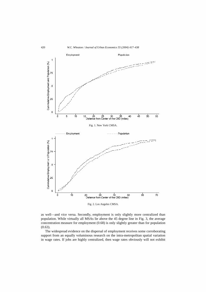
A more detailed analysis of job dispersal has recently become possible with the releaseof Commerce Department information on employment at place of work—by zip cGlaeser–Kahn [7] use this data to reestimate the employment density gradients oriobserved by Mills [17]. With zip code level data, however, it is possible to consthe exact cumulative spatial distribution of employment from the “center” of each MSAoutward. This can then be compared with the similar distribution for residence popuExamples of these two distributions are shown in Figs. 1 and 2, for the two areas in tthat are held up as representing “traditional” as opposed to “newer” cities: the New Yoand Los Angeles CMSAs. In New York, while employment is slightly more concentrthan population, the closeness of the two distributions is unexpected. In Los Angeldistributions of population and employment are virtually identical.

Comparing density gradients across different MSAs is complicated because a gradihas at least several different parameters. Instead, this paper proposes a single mhow “concentrated” the spatial distributions are in Figs. 1 and 2. One takes the areathe cumulative distribution—up to (say) the 98% point for population, and then dividthe distance at that point. Cities that are “fully” concentrated at single central pointa value of unity. A city with an employment density gradient that is inverse to disthas a value of 0.5. A city with uniform employment density has a value less than 0.5measure is thus:

Concentration=b∫

0

e(t)

bdt,

wheree(t) is a cumulative fraction of jobs (population) at distancet , b a distance at which98% of population live.

In Fig. 3, the value of this measure for both population and employment is sfor 120 MSAs (or CMSAs). Across these areas, either measure of concentration variesfrom about 0.5 to 0.75 depending on how dense and spread out the population. In“monocentric” city, in which all jobs were within say the first 5 miles (out of 50),employment concentration metric would be close to 0.95 and the population valuthan 0.5. There are no cities like this.

Two conclusions are apparent. First, there is a remarkably close correlation bethe two measures(R2 = 0.73). Cities in which population is more spread out—jobs


thanragelation

ingnhibit

Fig. 1. New York CMSA.

Fig. 2. Los Angeles CMSA.

as well—and vice versa. Secondly, employment is only slightly more centralizedpopulation. While virtually all MSAs lie above the 45 degree line in Fig. 3, the aveconcentration measure for employment (0.68) is only slightly greater than for popu(0.63).

The widespread evidence on the dispersal ofemployment receives some corroboratsupport from an equally voluminous research onthe intra-metropolitan spatial variatioin wage rates. If jobs are highly centralized, then wage rates obviously will not ex


agesutingts [5],

tontion ist rentcaseexact

ialch

g andestsr.es can

ant

Fig. 3. Employment and population centralization (120 MSAs).

much spatial variation. However, as will be discussed below, with job dispersal, wratesmust vary by location in a manner that exactly compensates workers for commto alternative job sites. There is a growing documentation of such variation: EberMadden [16], Ihlanfeldt [12], McMillen–Singell [13], Timothy–Wheaton [23].

3. “Mixed” land use and commuting

In order to model dispersed employment, the city constructed here will continuebe circular with location defined as being distancet from some geographic “center.” Ithe traditional theory of competitive spatial markets, land use at each such locaexclusively of one type—deterministically based on which use offers the highes(Alonso [1]). By definition this precludes land use mixing, except possibly in thewhere the rent from two uses is identical. Even in the case where rents are “tied,” thefraction of land that is assigned to each use isundetermined. As a result, traditional spattheory tends to create land use patterns in which there are exclusive zones or rings for eause. With rings or multiple employment zones determining the pattern of commutinrents becomes extremely complex.1 Furthermore, the evidence in Figs. 1 and 2 suggthat employment is sufficiently diffused so that exclusivity of use may in fact rarely occu

As an alternative, this paper adopts the convention of assuming that different uscohabit the same location. The fraction of land at each location that is commercial,F(t),

1 In Braid [4], it is assumed that when rents are “tied”the fraction of land used by employment is constand equal to the aggregate land share.


tion

ies,

enousre.

e

e” or

ose,

mberheer ofit alsoand

severalticular

rsence

can vary continuously over the 0–1 interval while the remaining fraction, 1− F(t) isdevoted to residential use.

A simplification in the current model will be the assumption that the consumpof land (per worker), both at both at their place of employment(qf ) as well as at thelocation of their residence(qh) be fixed and independent of location. In most modern citworkplace land consumption is far smaller than residential(qf � qh), but this is only anobservation and is not necessary for the model at hand. Allowing density to be endogcomplicates the model, but should not changethe qualitative conclusions derived heIn any case, it will be one of several suggested future extensions.

With fixed density at both residence and workplace,e(t) andh(t) are defined as thcumulative number of workers or households who liveup to the distance t . Using theF(·)function from above, these are:

e(t) =t∫

0

2πxF(x)

qf

dx, (1)

h(t) =t∫

0

2πx1− F(x)

qh

dx. (2)

The spatial distribution of employment and households will have an outer “edglimit. No jobs exist beyond the distancebf and no households beyond the distancebh. Thetwo edge distancesbf andbh are determined so that the cumulative distributions at thpoints equal the exogenous number of jobs and households [E andH ]. For conveniencethe equality between total jobs and households is assumed:

e(bf ) = E = H = h(bh), e(0) = 0 = h(0). (3)

An important assumption, that thetransportation technology allows only inward radialcommuting, results in a very simple and easy characterization of traffic flows. The nuof commuters passing each distance in the cityis equal to the difference between tcumulative number of workers employed up to that point and the cumulative numbresidents living up to that same distance. Since reverse commuting is not allowed,follows that workplaces must not be “more dispersed” than residences. Thus the dem(flow) of inward-only commutersD(t), under this assumption is:2

D(t) = e(t) − h(t) � 0, (4)

D(bh) = D(0) = 0,

bf � bh [sobh is the urban boundary]. (5)

These assumptions generate a resulting pattern of travel demand that hasinteresting features. First off, it is clear that there exists a land use pattern (a par

2 If each household has only one job and each job is filled by only one household, and there is no revecommuting, thenD(t) < e(t) − h(t) would imply that there is excess labor demand somewhere up to distat ,and excess labor supply beyondt . The reverse implies the opposite inconsistency. Finally, ife(t) − h(t) < 0 thenthere are more jobs beyondt than residences and reverse commuting must be occur.


f land

lwhere

d

ents

at theeree cost

ty can

s areestionvenoted

t ories,8] andsame

ges of

tion

itional

function F(t)) for which there isno commuting. If at all distancest , e(t) = h(t), thentravel demand is everywhere zero. Using (1) and (2), this is the case if the fraction oused by firms is always equal to their “share” of overall land demand:

F(t) = qf

qf + qh

, implies e(t) = h(t) for all t, and bf = bh. (6)

A second observation is that when the land use patternF(t) does generate travedemand, then travel demand is at a (local) maximum or minimum at that distancethe marginal number of household equals the marginal number of jobs:

D(t) reaches a local maximum where1− F(t)

qh

= F(t)

qf

. (7)

Equation (7) implies that ifqf is much smaller thanqh, then maximum travel demantends to occur near to whereF(t) goes to zero—at the edge of employmentbf , regardlessof how dispersed that employment is. At this point in the city, the number of residtraveling inward is very high, since no one has yet to be “dropped off” at work.3

Finally, travel demand must be converted into travel costs. It is assumed thmarginal cost of travel has a fixed component(β), as well as endogenous congestion. Han amended version of the Solow [22] congestion function is used wherein the timper mile is proportional to demand and inverse to capacity,S(t):4

∂C(t)/∂t = C′(t) =[

D(t)

S(t)

]α

+ β. (8)

Again, for the sake of simplicity, this model assumes that transportation capacibe provided without using up land and soS(t) implicitly reflects only road “capital.” Thiskeeps the number of urban land uses to just two (employment, residence).5

4. “Optimally” mixed land use when there is urban agglomeration

If the only spatial impact of location choices is on congestion then clearly citiemost efficient if jobs and people are perfectly interspersed—at which point conggoes to naught and travel costs have only theβ component. In fact, however, there haalways appeared to be additional costs associated with the location of production. Asby Mills [17], firms historically incurred shipping costs to and from a central portransportation terminal, often because water access was so important. In modern cithowever, trucking has made shipping costs more ubiquitous. Ogawa and Fujita [1Anas–Kim [2] have assumed that firms must contact or ship to all other firms in the

3 In conversation, William Vickery once observed that congestion was much worse around the edManhattan than at its center.

4 None of the results here are based on the congestion function having a coefficient ofα = 1, although thatwill sometimes be assumed in the simulation results. Actual studies (Small [21]) suggest that the ratio assumpis reasonable but withα > 1 (Small suggestsα = 2).

5 This model differs from that of Ogawa and Fujita [18] in two significant respects: they use the tradF = 0, 1 assumption which does not permit mixing, and they do not incorporate congestion.


eencosts ated someurban

r,leadtively,of theon.

ncethe cityons.tainallyented.

ial

nonefter.,

with

city and hence modeled intra-urban shipments as the aggregation of distances betwbusinesses. In a circular city, such a measure yields the least aggregate shippingthe center and the most at the edge. More generally, numerous authors have proposmore unspecified “urban agglomeration” factor that also works best at the densecenter (Glaeser–Kahn [7], Rouwendal [20]).

Whatever the source of the agglomeration, if firms are all located at one centeproductive efficiency will be highest or production costs lowest. This pattern will alsoto the longest commute trips and hence congestion will be greatest as well. Alternadispersed employment reduces congestion, but also productivity. The objectivecurrent model is only to examine the impact ofsuch agglomeration and not its generatiThus this model will assume some function for output/workerQ(t), which declines withdistance from the urban center. Greater agglomeration implies a steeper gradient. Makingthis gradient exogenous again provides great analytic simplicity.

With land consumption fixed, aggregate welfare in a city is simply the differebetween aggregate output and the aggregate cost of commuting determined fromcenter to edge(T ). To aid in the presentation, we make a few additional simplificatiThe first is that travel supply is constant and normalized toS(t) = S = 1. The second is thaβ = 0. Finally, we also assume that the land consumption of each use is the same and agequal to unity, that isqf = qh = 1. These simplify the presentation, but do not materichange the results. Later they will be relaxed when simulation results are presIncorporating these simplifications with (8), the objective function thus becomes:

maxF(t)

:

T∫0

2πtF (t)Q(t)dt −T∫

0

D(t)α+1 dt . (9)

Differentiating (4) with respect tot and applying (1) and (2) provides a differentequation that linksF(t) to changes in travel demandD(t):

D′(t) = 2πt[2F(t) − 1

]. (10)

Finally, F(t) andD(t) must be quite tightly constrained:

0 � F(t) � 1, 0 � D(t) � H, D(0) = D(T ) = 0. (11)

This greatly limits the set of feasible solutions. SinceD(0) = 0, D′(0) must be� 0or elseD(t) becomes negative. This in turn requires thatF(0) � 1/2. Similarly, to avoidnegativityD′(T ) � 0, which requires thatF(T ) � 1/2. In effect, the constrained solutioto F(t) must not slope upward. A traditional monocentric city will have a CBD zexclusively of firms, withF(t) = 1.0 over some initial distance and then zero thereaAt the other extreme, a fully dispersed city hasF(t) everywhere equal to 1/2. In-betweenemployment is more, but not completely, centralized relative to residences.

The problem in (9)–(11) represents a well-defined optimal control problem, albeitsignificant constraints. The Hamiltonian is

H = 2πtF (t)Q(t) − D(t)α+1 + λ(t)[2πt

[2F(t) − 1

]].


lity

alif

wing

n

)

o be

A solution to the problem involves two general conditions. First,F must optimizeH atall t , given the required constraints:

[2πtQ(t) + λ(t)4πt

]

� 0, if F(t) = 1,

� 0, if F(t) = 0,

= 0, if F(t) is within the 0–1 range.

(12)

The second condition that must hold everywhere with an equality is:

∂H/∂D(t) ≡ −(α + 1)D(t)α = −λ′(t), over allt . (13)

Thusλ(t) must be negative, but also non-decreasing (generally increasing) int .Equation (12) can hold as an equality if the optimalF(t) is in the interior of the

constraint range, as well as if it “runs along” either constraining value: 0, 1. A strictinequality can occur only at the constraint boundaries. When (12) holds with an equathen it can be differentiated: this equatesQ′(t)/2 with −λ′(t). Combining this result with(13) and then differentiated again yields the following.

Q′′(t)/2 = [−α(α + 1)D(t)α−1]D′(t)= [−α(α + 1)D(t)α−1][2πt

[2F(t) − 1

]]. (14)

Equation (14) can hold over any optimalF(t) that is feasible. However, if the optimsolution hasQ′(t)/2 ≶ −λ′(t), then (14) will not hold—and this can be true onlythe optimalF(t) is at the constraint boundaries. This observation provides the folloresults.

Proposition 1. Fully dispersed employment is never optimal with a negative productivitygradient.

Proof. Full dispersal of employment is possible only ifF(t) = 1/2 everywhere, whichthen generates aD(t) that is everywhere equal to zero. Hence from (13)λ′(t) = 0 andλ

must be a negative constant. ButQ(t) is not constant, and hence (12) implies thatF(t) willbe constrained at 1 and 0 asQ(t) is greater or less than 2λ. Thus it will be impossible forF(t) to have an interior solution (which must be the case if it everywhere equals 1/2). �Proposition 2. F(0) = 1.

Proof. Equation (11) requiresD(0) = 0. Thus ifQ′′(0) is either positive or negative theEq. (14) cannot hold att = 0. As discussed above, the only values ofF(t) where (14) willnot hold is at one of its two constrained values.F(0) = 0 is ruled out from (10) and (11and henceF(0) must equal one. �Proposition 3. If Q′(t) < 0 and Q′′(t) > 0 everywhere (e.g. a negative power orexponential function), then there must exist a CBD: an interval [0, t∗] where F(t) = 1.0.

Proof. Suppose over 0> t > t∗, F(t) declines gradually from 1 into the range[1/2 <

F(t) < 1], then (12) implies that Eq. (14) holds in this range. For the RHS of (14) t


gand

d usejobs.ticular

timalminetterns.

ralons.whereabout

mcts

mustl

positiveF(t) must be less than 1/2. Moving away fromt = 0,F(t) cannot be less than 1/2since this generates negativeD(t) values ast increases from 0. At somet∗, F(t∗) must“jump” from 1.0 to a value smaller than 1/2, from which it can decline smoothly.�Proposition 4. Mixed land use is possible everywhere except at t = 0 only if Q′′(t) < 0 forsome range of t < t∗ and Q′′ > 0 for t > t∗.

Proof. Mixed use requires (12) be an equality and hence (14) hold. To haveF ′(t) < 0over all t (so jobs are more centralized than residences) requiresF(t) > 1/2 for t < t∗.From (14) these necessitate thatQ′′(0) must be negative. At some pointt∗, F(t∗) = 1/2.From there outwardF(t) < 1/2 and (14) requiresQ′′ > 0. For there to be partial mixineverywhere,−Q′(t) must rise and then fall—matching the spatial pattern of traffic demD(t) which always does likewise. SimilarlyQ′′(t) must match up with−D′(t), being atfirst negative and then positive.�

These results are quite powerful for they seem to imply that fully interspersed lanis never optimal—agglomeration always gives rise to some degree of centrality ofFurthermore, “exclusive” central business zones are normally optimal unless the parpattern of agglomeration exactlymatches that of traffic demand.

5. Wage and rent gradients in a market model of mixed land use

The model above shows that with a range of “agglomeration” functions it can be opto have employment fully or at least “partially” centralized. The next step is to exahow a competitive private land market might produce a similar range of land use paThis necessitates determining market land rents.

With land consumption fixed, household utility dependsonly on net income aftereceiving wages, paying for travel costs, andconsuming land (paying rent). With identichouseholds, equilibrium then requires that net income be constant across locatiOf course in this model, households make two location decisions: where to live andto work. There thus must exist two “price” gradients to make households indifferenteach decision.

For households at a fixed place of residence,all alternative workplaces must yield theidentical net income. Since rent is fixed by residence place, choice of workplace impanet income through commuting. For indifference, a wage gradientW(t) must exist andvary directly with the marginal cost of travel:

∂W(t)/∂t ≡ W ′(t) = −C′(t), W(0) = W0. (15)

For households at a fixed place of employment, all alternative residential choicesbe equally attractive. This requires a land rent gradientRh(t) that varies with the marginacost of travel and everywhere is greater than the reservation rent for land(A), except at theedge of residential development:

∂Rh(t)/∂t ≡ R′h(t) = −C′(t)/qh, Rh(bh) = A. (16)


blerents

ientst likely,ientsge of

ationlly onf landallows

hestg ofsumingsame

craticm is

e two

rede

ve.ercialts. Inest use

de

Turning to firms, equilibrium will require that the location of jobs be equally profitaat all locations. Thus it must be true that worker productivity, wages and firm landall exactly offset each other. Thisyields a firm land rent gradientRf (t) that obeys thefollowing conditions:

∂Rf (t)

∂t≡ R′

f (t) =

Q′(t) − W ′(t)qf

,

Q′(t) + C′(t)qf

, from (9), Rf (bf ) = A.

(17)

Thus if the decline in productivity is larger than marginal travel costs, firm rent graddecrease with distance. From (7)–(8), the pattern of congestion suggests this is mosto occur at the very center (t = 0) and at the residential edge (t = bh). On the other handif marginal travel costs are larger than the decline in productivity, then firm rent gradmight increase with distance. Again from (7)–(8), this is most likely at or near the edemploymentbf .

Thus if Eq. (15) through (17) hold, both firms and households can be in locequilibrium. The rent and wage gradients that insure this, however, depend cruciacongestion, which in turn, depends on the travel flows that result from the pattern ouse mixing. Thus a rule is needed in which rents determine land use in a manner thatmixing.

It is clear that the traditional competitive assumption that land goes to its “higuse” will create perfect segregation of uses, or in the case of “ties” perfect mixinan undetermined degree. As an alternative, this paper adopts the convention of asthat there are random or idiosyncratic effects that allow different uses to cohabit thelocation. The fraction of land ateach location that is commercial,F(t) then will dependon therelative magnitude of the rent levels for each use.6

There are a number of functions that one could use to model some kind of “idiosynland use competition,” including for example logistic choice. Here a very simple forillustrated, again for analytic ease. The only requirement is that the functionF(t) map apair of positive values for commercial and residential land rents[Rf (t),Rh(t)] into thezero–one interval. The function in (18) assumes that with equal Ricardian rent, thuses get equal (50%) land use assignment:7

Equal rents imply equal shares:F(t) ={

Rf (t)/[Rf (t) + Rh(t)

],

0, if Rf (t) � A.(18)

6 There are two reasonable arguments that can be made for land use mixing: that there exists some unmeasu“other” location dimension, or that there are true random variations in utility or production. An example of thfirst would be the tendency of commerce to occupy the first floor of urban buildings while residences exist aboThe unmeasured impact of foot traffic in the vertical dimension generates this kind of “mixing.” Commpreferences for corners, frontage, etc. operate similarly. True random effects would generate stochastic renthis case, each use would have a probabilistic rent distribution for any location and application of the highprinciple would yield probabilistically mixed land use. See Anas [3] for a similar idea.

7 A simple alternative would beF(t) = qf Rf (t)/[qf Rf (t) + qhRh(t)]. Here, with equal rents land woulbe allocated in proportion to its aggregate usage. If the allocation is stochastic-based, however, it seems morreasonable to assume that with equal rents, eachuse stands an equal chance of acquiring land.


o uses.n be

ingend use

nts.mayabove.

tions of

lytose,equired usessible:

er allholds,

olds arerticular

of landuseidly

andl

hel. With

Thus if there are two non-negative rent gradients over the dimension(t), then the abovefunction can be used to determine the aggregate allocations of land to each of the tw

With the specification of the market assignment function, a positive model catheoretically “closed.” An equilibrium solution can be imagined with the followmappings. Equation (18) takes the two rent gradients[Rf ,Rh] and maps them with thF(t) function into land use shares at each location. Equations (1) through (8) take lashares and determine the pattern of travel[e(t), h(t),D(t), andC(t)]. Finally, Eqs. (15)through (17) take the pattern of travel congestion and map it back to the rent gradie

While it is quite straightforward to find reasonable equilibrium market solutions, itnot always be the case that one exists, at least without further restrictions than thoseA particular troublesome problem can arises for seemingly reasonable representaC(t) andQ(t). At points of maximum congestion it is possible thatC′ > −Q′ and firmbid rents will locally slope up with greater distance. Since according to (17) this is liketo happen near to the edge of employment, it can become difficult to find a solutionbf .

While it is difficult to prove that an equilibrium always exists with mixed land uit is quite easy to find particular market solutions, and to demonstrate that these rcertain conditions. As a first step, it is useful to examine the range of simulated lanpatterns that are possible with the equations from this section. Two patterns are popartially mixed use (over some range of locations), and fully mixed land use ovlocations (dispersed employment). In the first, firms are more centralized than housebut there is a range of locations where both uses exist. In the latter, firms and househperfectly and evenly intermingled. Each of these outcomes can be generated with pacombinations of urban productivity, transport capacity, and population size.

6. The dispersal of employment and agglomeration

When an idiosyncratic land use function is used, such as (18), then some degreeuse mixing occurs by definition. Thedegree of employment dispersal, and hence landmixing, however, will depend heavily on the level of agglomeration or on how rapproductivity declines with distance.

Proposition 5. Lower agglomeration generates greater employment dispersal in mixed usecities.

Proof by contradiction. In a city that has a partially mixed land use pattern,bf < bh,and F(t) < 1, for t < bf . With less agglomeration, the absolute value ofQ′(t) is lessat all locations.If greater employment centralization were to result, thenbf would haveto be smaller, requiringF(t) be higher over at least part of the interval[0, bf ]. From(1)–(8), however, this would causeC′ to be greater over this same interval. From (16)(17), lowerQ′ and higherC′ when combined with a smallerbf will reduce commerciarent levelsRf (t), and increase residential rentsRh(t) over this interval. With (18) thiswill reduce rather than increaseF(t) over t = 0, bf . Through the reverse argument, tconverse holds as well—greater agglomeration cannot lead to employment dispersa


ndary

nce ofet the

el

s

hilen alsog andessary”

ike ars),mption

ess zoneestione of thegeig. 5),to be

tult thatlandentral

tban

less agglomeration, firm rent gradients are flatter and the firm employment boufarther. �

At the extreme case, fully dispersed employment does not require the abseagglomeration, but rather only that agglomeration must be such as to exactly offsexogenous travel costs that occur when congestion is nil.

Proposition 6. A fully dispersed employment equilibrium is possible with the land use mixfunction (18).

Proof. Full employment dispersal requires thatF(t) = qf /(qf + qh) ande(t) = h(t) overall t . Hencebf = bh, D(t) = 0, andC′(t) = β (no congestion, only exogenous travcosts).

If the ratio C′/Q′ = −q2h/[q2

f + q2h], while C′ = β , and henceQ′ is constant acros

locations, as well, then all the gradients also have constant slopes:W ′(t) = −β , R′h =

−β/qh, andR′f = −βqf /q2

h = (qf /qh)R′h. Furthermore, it is necessary forA = 0, so that

rent levels become proportional to their slopes. Then using (18), ifF(t) = Rf (t)/[Rf (t)+Rh(t)], it is also true thatF(t) = qf /(qf + qh). �

The important assumption in this example is that for any given city, the ratioC′/Q′ isequal to the residential share of squared land consumptions across the two uses. Wthis may seem restrictive, it is actually quite realistic and other assumptions cagenerate a fully dispersed city. A most interesting point is that even with no commutincongestion, some rent and wage gradient based upon free-flow travel costs is “necto insure that employment and residential locations remain dispersed.

Figures 4–5 illustrate a mixed land use city that is extremely close to looking ltraditional centralized monocentric city. There are 2 million households (and workefirm land consumption is 0.0001 square miles per worker and household land consuis 0.0005 square miles per worker. Exogenous marginal transport costs are set toβ = 100and transportation capacity is set so as to be constant across distance. The businextends to ring 96 and the city edge is at ring 195 (rings are tenths of miles). Congis zero at the very center and residential edge, and reaches a maximum at the edgbusiness zone (Fig. 4) where congestion costs are approximately $350 per mile. This edis determined by where the firm rent gradient equals the reservation rent for land (Fand firm rents are based on a spatial decline in worker productivity that is assumedabout twice the maximum marginal travel cost(Q′ = −1200). This is sufficient so thafirm rent gradients are much steeper than those of households (Fig. 5). As a resportion of the city with mixed use (to ring 96) has on average almost 80% of itsused by firms. In this simulation, aggregate travel expenditures are 5.4 billion, and cresidential rents reach 105 million per square mile.8

8 In the top figure of each pair, population and employment depict the normalized variables:h(t)/H,e(t)/E.Travel costs areC′ = 25D(t)/S(t) + β. Transport capacity is set to be uniform overt : S(t) = 125600. Transporcosts are in yearly $/mile, and rents are in yearly $/square mile. The annual opportunity rent of land at the ur


ne intvotedthe) is ashalf

e

Fig. 4. Land use and travel costs, 2 million inhabitants, mixed use city, high agglomeration.

Fig. 5. Land rents, 2 million inhabitants, mixed use city, high agglomeration.

Figures 6–7 illustrate a similar mixed land use city, but one where the decliproductivity is a quarter as much,−300 as opposed to−1200 per mile. The employmenborder moves out (from 96 to 155) and the fraction of land inside this border that is deto commercial use decreases to an average of40%. Because of greater land use mixing,necessity to commute is lower, and thereby the marginal cost of travel (congestionwell. In the aggregate, travel expenditure is down sharply—to 2.5 billion—less than

edge isA = $1000000 per square mile. Finally, in various simulations worker productivity is assumed to declinlinearly with distance in the range:Q′ = −100 to−1200.


ion ist of thisrents

ree equal

withince no

Fig. 6. Land use and travel costs, 2 million inhabitants, mixed use city, low agglomeration.

Fig. 7. Land rents, 2 million inhabitants, mixed use city, low agglomeration.

of its value in the more centralized city (Figs. 4–5). Part of this expenditure reductdirectly due to less aggregate travel, with the remainder due to the secondary impacon the marginal cost of travel. With lower marginal travel costs, central residentialdrop, here to 78 million.

Finally in Figs. 8–9, a city with fully dispersed employment is illustrated. This is simplyaccomplished by setting the level of agglomeration at that specified in Proposition 6. Theis no commuting and hence no congestion, so marginal travel costs everywhere arto β = 100. At each location, firms occupy 17% of land and residences 83%. Evenexogenous marginal travel costs, aggregate travel expenditures are equal to zero s


a large

educesd rent.llion,

nrtial

Fig. 8. Land use and travel costs, 2 million inhabitants, fully dispersed city.

Fig. 9. Land rents, 2 million inhabitants, fully dispersed city.

one has to travel! In the fully dispersed city, the absence of congestion generatesdifference in land rents—central residential rents now are only 37 million.9

These three simulations show how lower agglomeration disperses employment, rcommuting and hence congestion costs and thereby reduces residential lanCommercial land rents also are greatly reduced, from 700 million down to only 7 mi

9 The mixed use city simulations in Figs. 4–7 use the sameF(t) function as in the fully dispersed simulatioresults of Figs. 8–9. Only the values of agglomeration and exogenous travel costs are changed, so that pamixing occurs rather than fully dispersed employment.


s thege andtravel,ersed.

ient are

es inl uses,s and

e

pects

d thetral

’ para-ures—n

gregatee ofosts,er but.7 bil-

ng,ity

here

but much of this is due directly to the reduction in agglomeration that generateincreasingly more dispersed employment patterns. It is interesting that both a warent gradients continue to exist in the fully dispersed city—even though there is noand congestion is absent. This is to insure that firms and households remain fully dispAs long as travel has some cost—even without congestion—a wage and rent gradnecessary to keep economic agents completely interspersed.

7. The dispersal of employment and transportation capacity

While changes in agglomeration alter the slope of a firm’s rent gradient, changtransportation capacity alter the rent gradients for both commercial and residentiathrough impacting congestion. As expanded capacity improves travel flows, both firmresidences move further “apart” torealize other location advantages.

Proposition 7. Expanded transport capacity generates employment centralization.

Proof by contradiction. In a mixed land use pattern,bf < bh, andF(t) < 1, for t < bf .With a uniform expansion ofS(t), and no change in land use,C′(t) will decreaseeverywhere. From (16)–(17), this causesR′

f to increase at all locations, whileR′h is less at

all locations. With fixed aggregate land consumption, the urban boundarybh is fixed andthusRh(t) will be lower at all locations.Suppose bf were to increase, thenRf (t) would behigher at all locations. From (18), these rent changes would causeF(t) to be greater at thsame time thatbf increases—violating (1). To meet conditions (1)–(2),bf must contractasF(t) increases—the definition of employment centralization.�

Figures 10–11 illustrate a simulated city with mixed employment that is in all residentical to that in Figs. 6–7, except that the value of transport capacityS(t) has beendoubled at each location. The employment border moves in (from 155 to 128) anfraction of land inside this border that is devoted to commercial use increases. Cencommercial rents increase whileresidential rents decrease.

The land use changes in Figs. 10–11 provide an interesting version of “Braessdox”: adding transportation capacity may actually increase average travel expenditin the absence of congestion-based user pricing (Small [21]).10 In the base case simulatioof Figs. 6–7, marginal travel costs per mile are higher, but job dispersal keeps the agmiles of travel low. The combination of the two generates aggregate travel expenditur2.5 billion. By adding capacity, the city in Figs. 10–11 has lower marginal travel cbut the more centralized land use pattern leads to longer trips. The product of longspeedier travel actually leads to greater travel expenditure—about 10% higher, at 2lion. With the same population, average trip times are higher as well.

10 If each driver’s actions are based on minimizing total system costs, as they would be with congestion pricithen the envelope theorem applies and the general equilibrium impact on total system costs of adding capacequals the partial impact—always beneficial. In the real world, where efficient congestion pricing is absent, tare many documented examples of the paradox.


y.

reasedrkingpolitan

Fig. 10. Land use and travel costs, 2 million inhabitants, mixed use city, expanded transport capacit

Fig. 11. Land rents, 2 million inhabitants, mixed use city, expanded transport capacity.

8. The dispersal of employment and travel demand

Increasing travel demand occurs in the real world for any number of reasons: inccar ownership with greater income, a rise in the proportion of households with two woheads, etc. In this model we increase travel demand my expanding the metropopulation—while keeping the urban boundary fixed. In effect,E andH increase throughcomparable decreases inqh andqf (increased density), whilebh andbf remain fixed. This


ply

ither

f

Fig. 12. Land use and travel costs, 1 million inhabitants, mixed use city, low agglomeration.

Fig. 13. Land rents, 1 million inhabitants, mixed use city, low agglomeration.

will proportionately increase the aggregatenumber of commute trips each day. The supof transportation capacity remains fixed.

Proposition 8. Increased travel demand (greater density) generates greater employmentdispersal.

Proof by contradiction. Consider starting from a city whose land use pattern is nefully dispersed nor fully centralized. In this casebf < bh, andF(t) < 1, for t < bf . IfE and H expand internally by a factor(γ > 1), becauseqh and qf decrease by 1/γ ,then at eacht , e(t), h(t) and the differenceD(t) grow by γ . Without any expansion o


att

),

s halftotalof the

d thusr, but2–13,n inin

worse.

tweenobtaintion.with

ctlyrticular

list ofined,ge jobives anption

studied

. Jobuting

tonatternr [19]l. Theiraverage

cityn their

travel capacity,C′(t) increases everywhere. Together with the scaled decreases inqf , qh,this causesR′

f to decrease relative toR′h at all locations (in absolute value). Given th

bh is fixed, and thatbf < bh, this reducesRf (t) relative toRh(t). From (18), these renchanges would causeF(t) to be less at all locations up tobf . To meet conditions (2)–(3bf must expand asF(t) is lower. An expansion ofbf and decrease inF(t) for t < bf isthe definition of greater employment dispersal.�

Figures 12–13 illustrate a simulated city with a mixed land use pattern that hathe population, but also half the density levels, of the city in Figs. 6–7. Since theland consumption of each use is the same, so will be the outer residential edgecity. However, the increase in population and density (moving from Figs. 12–13backto Figs. 6–7) causes the employment boundary to increase from 126 to 155, anthe employment distribution to flatten. Congestion is everywhere slightly greateemployment dispersal leads to shorter trips (Gordon–Richardson [8]). In the Figs. 1aggregate travel expenditure is 1.37 billion, which is more than half of the 2.5 billioFigs. 6–7. Thus the employment dispersal that accompanies the (two-fold) increasestravel demand leads to lower average travel expenditure even though congestion is

9. Conclusions and extensions

It is tempting to conclude from the results above that there is a divergence bemarket outcomes and optimal land use. In the market simulations it is easy tofully dispersed employment using a simple linearly declining agglomeration funcIn this case, however it is never optimal to have jobs completely dispersed. Norlinearity is it optimal to have “smooth” mixing. The problem, however, is that direcomparing the two models is somewhat misleading, since the market model has a pa“idiosyncratic” mixing function—which the optimal model does not.

The paper has only begun to analyze cities where land use mixing can occur. Theextensions is quite long. First off, more realistic two-way commuting might be examsince clearly all travel modes have this feature. This would seem to further encouradispersal. Next, density or land consumption could be made endogenous, and this gadditional dimension of adjustment to job dispersal decisions. Private land consumdecisions by households are not efficient, and the residential case has been well(Wheaton [25]), but the density decision of firms should impact congestion as well.

The empirical implications of the model, however are perhaps most interestingdispersal per se should, if the model is correct, lead both to lower marginal commcosts as well as travel distances. There are two pieces of research on this question. Hamil[10] first argued that cities do have very dispersed employment—and that the pwas inconsistent with the observed high commuting times. Richardson and Kumaundertake a more thorough statistical analysis using a rough measure of job dispersacross section results show that more dispersed cities, ceteris paribus, do have lowercommute times. Both papers, however take observed employment dispersal asexogenous.

In a follow up paper to their original model, Fujita and Ogawa [6] argue that aspopulation increases and traffic congestion worsens, there is a greater likelihood (i


r trafficyment

ongerces trip

en acitiesters

theloymentmineedortante speed

0

ed,

988)

81)

ns,

. Gale,

th:02.(2)

91)

urnal

l of

Eco-

Eco-

01.

al

model) of a second employment center forming. In the model developed here, greatecongestion (through increased demand or reduced supply) leads directly to emplodecentralization. Thus in any cross section of US cities, it may be equally likely that ltrip times produce employment dispersal as well as that dispersed employment redulengths.

To overcome this shortcoming, McMillen and Smith [15] have recently undertaksimilar cross section analysis of city employment dispersal. They find that largerand cities whereinstrumented travel demand is higher do in fact have more subcen(such as Fujita predicts). This finding corroborates as well the comparative statics ofmodel here, wherein such differences generate a greater degree of continuous empdispersal. Clearly further empirical work is needed. It is important to not only deterif instrumented travel demand causes employment dispersal, but also if instrumentemployment dispersal reduces travel. In the latter question, it also would be impto determine if job dispersal independently reduces trip distances and/or the averagof travel.

References

[1] W. Alonso, Location and Land Use, Harvard Univ. Press, Cambridge, MA, 1964.[2] A. Anas, I. Kim, General equilibrium models of polycentric land use. . . , Journal of Urban Economics 4

(1996) 232–256.[3] A. Anas, Taste heterogeneity and urban spatial structure: The logit model and monocentric theory reconcil

Journal of Urban Economics 28 (1990) 318–335.[4] R.M. Braid, Optimal spatial growth of employment and residences, Journal of Urban Economics 24 (1

227–240.[5] R.W. Eberts, An empirical investigation of urban wage gradients, Journal of Urban Economics 10 (19

50–60.[6] M. Fujita, H. Ogawa, Multiple equilibria and structural transition of nonmonocentric urban configuratio

Regional Science and Urban Economics 12 (1982) 161–196.[7] E. Glaeser, M. Kahn, Decentralized employment and the transformation of the American city, in: J

W. Pack (Eds.), Papers on Urban Affairs, Brookings Institution, Washington, 2001, pp. 1–65.[8] P. Gordon, H. Richardson, Transportation and land use, in: Holcombe, Staley (Eds.), Smarter Grow

Market Based Strategies for Land Use Planning in the 21st Century, Greenwood Press, Westport, CT, 20[9] G. Guiliano, K. Small, Subcenters in the Los Angeles region, Regional Science and Urban Economics 21

(1991) 163–182.[10] B.W. Hamilton, Wasteful commuting, Journal of Political Economy 90 (1982) 1035–1053.[11] R. Helseley, A. Sullivan, Urban subcenter formation, Regional Science and Urban Economics 21 (2) (19

255–275.[12] K.R. Ihlanfeldt, Intraurban wage gradients: evidence by race, gender, occupational class, and sector, Jo

of Urban Economics 32 (1992) 70–91.[13] D.P. McMillen, L.D. Singell Jr., Work location, residence location, and the urban wage gradient, Journa

Urban Economics 32 (1992) 195–213.[14] D.P. McMillen, J. McDonald, Suburban subcenters and employment density, Journal of Urban

nomics 43 (2) (1998) 157–180.[15] D.P. McMillen, S.C. Smith, The number of subcenters in large urban areas, Journal of Urban

nomics 53 (3) (2003) 321–338.[16] J.F. Madden, Urban wage gradients: Empirical evidence, Journal of Urban Economics 18 (1985) 291–3[17] E.S. Mills, Studies in the Structure of the Urban Economy, Johns Hopkins Press, Baltimore, 1972.[18] H. Ogawa, M. Fujita, Equilibrium land use patterns in a non-monocentric city, Journal of Region

Science 20 (1980) 455–475.


Urban

(1)

nal

state

98)

3.of

[19] H. Richardson, G. Kumar, The influence of metropolitan structure on commuting time, Journal ofEconomics 27 (3) (1989) 217–233.

[20] J. Rouwendal, Search theory, spatial labor markets and commuting, Journal of Urban Economics 43(1998) 25–51.

[21] K.A. Small, Urban Transportation Economics, Harwood Academic, Philadelphia, 1992.[22] R. Solow, Congestion costs and the use of land for streets, Bell Journal 4 (2) (1973) 602–618.[23] D. Timothy, W.C. Wheaton, Intra-urban wage variation, commuting times and employment location, Jour

of Urban Economics 50 (2) (2001) 338–367.[24] P. Waddell, B. Berry, W. Hoch, Residential property values in a multinodal urban area, Journal of Real E

Finance and Economics 7 (2) (1993) 117–143.[25] W.C. Wheaton, Land use and density in cities withcongestion, Journal of Urban Economics 43 (2) (19

258–272.[26] M.J. White, Firm suburbanization and urban subcenters, Journal of Urban Economics 3 (1976) 232–24[27] M.J. White, Location choice and commuting behavior in cities with decentralized employment, Journal

Urban Economics 24 (1988) 129–152.

commuting, congestion, and employment ... - mit economics

Documents