community phylogenetics of forest trees along an ... · community phylogenetics of forest trees...
TRANSCRIPT

Community phylogenetics of forest trees along an elevational gradient in the eastern Himalayan
region of northeast India
Stephanie Shooner
A Thesis
in
The Department
of
Biology
Presented in Partial Fulfillment of the Requirements
for the degree of Master of Science at
Concordia University
Montreal, Quebec, Canada
November 2015
© Stephanie Valerie Shooner, 2015

This is to certify that the thesis prepared
By: Stephanie Shooner
Entitled: Community phylogenetics of forest trees along an elevational gradient in the
eastern Himalayan region of northeast India
and submitted in partial fulfillment of the requirements for the degree of
Master of Science (Biology)
complies with the regulations of the University and meets the accepted standards with respect to
originality and quality.
Signed by the final Examining Committee:
Chair
Dr. J. Grant
Examiner
Dr. G. Brown
Examiner
Dr. J. Jaeger
Examiner
Dr. J-.P. Lessard
Supervisor
Dr. S. Dayanandan
Supervisor
Dr. T.J. Davies
Approved by
Dr. S. Dayanandan, Graduate Program Director
Date:
Dean of Faculty
iii
Abstract
Community phylogenetics of forest trees along an elevational gradient in the eastern
Himalayan region of northeast India
Stephanie Shooner
Large-scale environmental gradients have been invaluable for unravelling the processes shaping
the evolution and maintenance of biodiversity. Gradients provide a natural setting to test theories
about species diversity and distributions within a landscape with changing biotic and abiotic
interactions. Elevational gradients are particularly useful because they often have an extensive
climatic range within a constricted geographic region. Arunachal Pradesh is the northeastern-
most province in India, located on the southern face of the eastern Himalayas. This region is
considered a biodiversity “hotspot”, with an estimated 6000 flowering plant species of which 30-
40% are endemic. For this thesis, I analyzed tree communities in plots distributed throughout the
province using both species and phylogenetic diversity indices. I explored shifts in community
structure across elevation and space as well as the biotic and abiotic forces influencing species
assembly throughout the landscape. Species richness and phylogenetic diversity decreased with
increasing elevation, as theory predicts. However, species relatedness did not show a clear
pattern with elevation. Nonetheless, by exploring beta-diversity (both taxonomic and
phylogenetic), I was able to show a strong effect of environmental filtering with elevation.
Environmental filtering is generally associated with species clustering on the phylogeny, where
co-occurring species in a community are more closely related than expected by chance. Here,
however, I suggest that forest community structure is driven by filtering on glacial relicts,
resulting in random or over-dispersed community assemblages. These patterns point to possible
regions for conservation priority that may provide refugia for species threatened by current
warming trends.

iv
Acknowledgements
I would first like to thank my supervisor Dr. Selvadurai Dayanandan for accepting me into his
lab, supporting and guiding my Master’s work. I was fortunate to have support from a second
supervisor, Dr. Jonathan Davies, who I would like to thank not only for inspiring me to pursue
this degree but also for providing endless guidance, grammar help and wild ideas. I would like to
thank Dr. M. L. Khan and the researchers at NERIST for providing me with access to this
incredible data set. I would also like to thank my committee members Dr. Jean-Philippe Lessard
and Dr. Jochen Jaeger for their constructive criticism and for keeping me on track.
I would like to extend a very special thank you to my mentor Chelsea Chisholm, who has
been my friend and role model since the very beginning, and to Ria Ghai for her kind heart,
hospitality and amazing scientific communication advice. Thank you to Tammy Elliott, Ignacio
(Nacho) Morales-Castilla, Maxwell Farrell, Hercules Araclides, Will Pearse and Sofia Carvajal
Endara for insightful conversations, help with R and for going along with my team building
ideas. Thank you to the Dayanandan Lab: Baharul Choudhury, Atiqur Barbhuiya, Mohammed
Atif-Zayed, Shiva Prakash and Sachin Naik for your kindness and support. I acknowledge the
endless list of colleagues at both McGill and Concordia that encouraged me to step out of the lab
every once in a while. I would also like to thank the researchers at the North Eastern Regional
Institute for Science and Technology who collected the data and made this project possible.
Most importantly, I would like to thank my family and friends for helping me keep things
in perspective. To my parents, thank you for providing warm meals, laundry, love and pep talks
whenever I needed them. To my sister Julie, thanks for being my number one partner in crime.
Last but not least, I thank my friends here, and all over the world, for keeping me busy.
This project was made possible by funding from the Quebec Center for Biodiversity
Science, Concordia University and the Natural Science and Engineering Research Council of
Canada.

v
Table of Contents
List of Tables ................................................................................................................................. vi
List of Figures ............................................................................................................................... vii
List of Supplementary Materials .................................................................................................. viii
PART I: Introduction .......................................................................................................................1
Brief history of phylogenetics ..............................................................................................1
Improving phylogenies ........................................................................................................2
Patterns in community phylogenetics ..................................................................................3
Dimensions of diversity and phylogenetic metrics ..............................................................3
Caveats and assumptions .....................................................................................................6
Phylogenetic community ecology along the elevational gradient .......................................8
Objectives and predictions .................................................................................................10
PART II: Phylogenetic diversity patterns in Eastern Himalayan forests reveal strong evidence for
environmental filtering of evolutionarily distinct lineages ............................................................12
Introduction ........................................................................................................................13
Methods..............................................................................................................................16
Results ................................................................................................................................18
Discussion ..........................................................................................................................20
PART III: Conclusions and future research ...................................................................................24
Figures............................................................................................................................................28
Tables .............................................................................................................................................31
References ......................................................................................................................................32
Supplementary Material .................................................................................................................41

vi
List of Tables
Table 1: Linear models testing change in LCBD and PLCBD with elevation and distance .........31

vii
List of Figures
Figure 1: Map of the study site in Arunachal Pradesh, India .........................................................28
Figure 2: Map of the spatial distribution of LCBD and PLCBD and the change in local
contribution to beta diversity with elevation .................................................................................29
Figure 3: The relationship between phylogenetic beta diversity and Sorenson’s beta diversity ...30

viii
List of Supplementary Materials
Appendix 1: Assessing sensitivity of results to differences in species identification among plots
........................................................................................................................................................41
Appendix 2: Genbank accession numbers for phylogeny reconstruction ......................................44
Appendix 3: Example phylogeny...................................................................................................50
Appendix 4: The relationship between the standardized effect size of phylogenetic diversity and
elevation .........................................................................................................................................51
Appendix 5: The net-relatedness index with gymnosperms and ferns removed ...........................52
Appendix 6: Mantel tests for phylogenetic beta diversity against elevation and distance with
gymnosperms and ferns removed ..................................................................................................53

1
PART I: Introduction
One of the most important questions in ecology is why some species occur where they do and
not elsewhere. The answer to this question is not a simple one; it encompasses a seemingly
endless list of factors and their putative interactions. Important within this list are climate,
elevation, species × species interactions, energy availability, and the adaptiveness of a given
species. There are various analytical approaches that consider these factors either separately or in
some combination, and often within an ecological gradient. In this thesis I explore one approach
in particular, the relatively new field of phylogenetic community ecology (community
phylogenetics). First described in detail by Webb et al. in 2002, community phylogenetics aims
to capture the interaction among species assemblages, phylogeny and traits. In the following
work I focus on the interface between species assembly and phylogeny, drawing inference from
the phylogenetic structure of the species present in a community assemblage.
Brief history of community phylogenetics
The field of community phylogenetics built on previous ideas of species co-occurrence
(Cody and Diamond 1975, Connor and Simberloff 1979, Gotelli and Graves 1996, Gotelli 2000),
and merged this with advances in phylogenetic theory. Among the first to hypothesize about the
nature of biotic interactions (species × species interactions), Darwin (1859) suggested that
species from the same genus would experience stronger competition than more distantly related
species from different genera on the basis that those species from the same genus were more
ecologically similar due to their shared evolutionary history. Many years later, Elton (1946)
empirically tested Darwin’s hypotheses by examining species-genus ratios in various
communities and found that the different genera present in the communities were rarely
represented by more than one species. He thus inferred that competition may allow different
genera of the same trophic level to coexist, but limited coexistence of species of the same genus.
Elton was also careful to suggest that it was necessary to distinguish between the ability of an
individual to exist in a given environment and the ability to persist within a particular species
assemblage. These ideas captured the essence of environmental filtering and limiting similarity

2
among related species as well as early ideas of niche filling within a community. Environmental
filtering is the process by which abiotic factors structure species assemblages. At large scales,
environmental filtering is thought to be a major determinant of species range, while at small
scales it can contribute to niche heterogeneity (e.g. through variable soil or moisture).
Conversely, limiting similarity describes the biotic interactions that can structure species
coexistence. If species are sufficiently similar in their resource-use (niche) or phenotypic
features, it is often presumed that they cannot coexist. Environmental filtering and biotic
interactions can be inferred from patterns of phylogenetic relatedness, discussed below.
The implementation of pairwise co-occurrence matrices improved understanding of the
theory of limiting similarity by allowing researchers to identify pairs of species that rarely or
never occurred together, providing an important step towards identifying the processes
responsible for the competitive exclusion of species within the environment (Cody and Diamond
1975). However, early results proved controversial as patterns were not compared to any null
expectation, and thus remained largely descriptive. With the development and popularization of
null models, these patterns in species assembly could be rigorously tested against a null
hypothesis of random species associations (Gotelli and Graves 1996). These crucial milestones
within ecology provided the foundation from which present-day community ecology and
phylogenetic theory emerged.
Improving phylogenies
Another important factor in the development of modern community phylogenetics was the
improvement of sequencing technology that allowed for better phylogenetic reconstructions.
Traditionally estimated from shared phenotypic traits, phylogenies are now quantifiable using
sequence information and fossil calibrations to inform divergence times among clades. With the
advent of PCR in the 1980s, and more recently, next generation sequencing technology,
molecular data can be generated quickly and cheaply, making the phylogenetic reconstruction of
many 100’s or even 1,000’s of species possible (e.g. Plants: Davies et al. 2004, Mammals:
Bininda-Edmonds et al. 2007; Birds: Jetz et al. 2012; Zanne et al. 2014; Animals, plants and
microbes: Hinchliff et al. 2015). These phylogenetic trees provide the raw material upon which
the indices describing community structure are based. The improvement of sequencing
technology also came with a growth in bioinformatics and computing power, allowing for the

3
development of analytical programs that could easily integrate evolutionary information (via
phylogeny), community information and sophisticated statistical tests.
Patterns in community phylogenetics
In a seminal paper, Webb et al. (2002) reviewed and discussed the potential for phylogenetics in
studies of community assembly and introduced the field of modern community phylogenetics.
The authors suggested that the distribution of pairwise distances measured on a phylogenetic tree
between species within a community could help elucidate the processes structuring community
assembly. It was hypothesized that communities structured by the abiotic environment would
include species that are more closely related than expected by chance, presenting as “clustered”
on the phylogeny. Under this scenario, a clustered community structure suggests that the species
present in a community share the same traits related to persisting in a particular environment,
assuming such traits are evolutionarily conserved. By contrast, a community structured by
competition would have species that are more distantly related than expected by chance, referred
to as “over-dispersed” on the phylogeny, again assuming trait evolutionary conservatism. Over-
dispersion is thought to be driven by competition for resources acting on conserved traits (i.e. the
traits that describe the fit of a species to its abiotic niche are conserved on the phylogeny), where
closely related species can undergo competitive exclusion stemming from the exploitation of
similar resources (Wiens and Graham 2005, Losos 2008). However, Webb et al. (2002)
acknowledge that an over-dispersed pattern could also suggest abiotic filtering, selecting for
converged traits across many clades, and other more recent studies have suggested similar
patterns of over-dispersion of clustering could arise from multiple processes (see ‘Caveats and
assumptions’, below).
Dimensions of diversity and phylogenetic metrics
There are several metrics for quantifying phylogenetic diversity patterns across a landscape, with
new methods being continuously developed in the field. Below, I describe some commonly used
metrics that I explored in the thesis.
Alpha diversity
RH Whittaker (1960) was the first to explicitly describe the three spatial dimensions of species
diversity in a landscape: alpha, beta and gamma diversity. He proposed that the total species
4
diversity of a region is equal to the sum of diversity per habitat in the region and the differences
in diversity among those habitats. In this thesis, I examine a relatively large region but assume a
single species pool, defined as the sum of all the species recorded in the study plots; I thus focus
on alpha and beta diversity, using both species and evolutionary information.
Phylogenetic diversity
Phylogenetic diversity (PD) was first described in the context of conservation prioritization,
particularly for areas where knowledge of the species pool was limited. Faith (1992) outlined the
challenges in determining priority from taxonomic diversity, namely that information on the
diversity of characters represented within a community was often lacking due to our limited
ecological knowledge on species in any given area or within any given clade—a problem that
remains today. Calculating evolutionary distances among species could instead, it was argued,
predict character diversity without quantitative measurements of those features (Faith 1992).
Phylogenetic diversity is presently and generally calculated using molecular phylogenies to
capture the evolutionary distances separating species. Several metrics of phylogenetic diversity
have been developed (e.g. see Schweiger et al. 2008, metrics reviewed in Winter et al. 2013);
this thesis uses Faith’s PD, defined as the sum of the total phylogenetic branch lengths, including
the root, for the species in a given community.
Species richness and phylogenetic diversity have been shown to be tightly correlated;
communities with high species richness will also have proportionately higher PD (Schweiger et
al. 2008). Incorporating a null model with the calculation of PD can disentangle phylogenetic
diversity from species richness—revealing whether a community contains more or less
evolutionary history than expected given its richness, helping distinguish between biotic and
abiotic processes structuring a community. Standardized metrics of PD can also control for
differences in species richness across samples (Proches et al. 2006).
Net-relatedness index
Similar to PD, the net-relatedness index (NRI) measures the standardized effect size of the
relatedness of species within a community by comparing observed relatedness to expected
relatedness given community species richness. More specifically, the net-relatedness index is
equal to -1 times the standardized effect size of the mean pairwise distance among species. The

5
NRI of a community can be positive (clustered) or negative (over-dispersed) and centers around
zero (random relationship among species). Values greater than 1.96 and less than -1.96 represent
those that are two standard deviations from a mean of zero and can be indicative of significance
(alpha=0.05), although significance testing is often formally assessed using randomizations. As
discussed briefly above, species communities that are phylogenetically clustered are generally
interpreted as being structured by the environment, where the traits important for persistence are
conserved among closely related species. Conversely, communities that are phylogenetically
over-dispersed are usually interpreted as being structured by competitive exclusion, where
closely related species exploit similar niche spaces and therefore cannot co-exist. This metric is
useful for exploring species assemblages in diverse or under-studied areas because it does not
require extensive collection of trait data and can provide some insight into the relative strength of
the biotic and abiotic factors structuring communities.
Beta diversity
Beta diversity, or turnover, is the difference in species composition across space. It can be
calculated in a variety of ways to determine boundaries in species composition or the rate of
change through space. Differences among communities can be analogous to the degree of
similarity between communities and the conversion between similarity and dissimilarity is
simple (dissimilarity = 1- similarity). In this thesis I calculate taxonomic beta diversity using
Sorenson’s index (eq. 1):
𝐸𝑞. 1: 𝑆𝑜𝑟𝑒𝑛𝑠𝑜𝑛′𝑠 =2𝐶
𝐴 + 𝐵
where A is the number of species in habitat A, B is the number of species in habitat B and C is
the number of shared species between both habitats. The phylogenetic equivalent of Sorenson’s
index is phyloSor, a measure of the shared branch lengths between habitats. The equation for
phyloSor is the same as Eq. 1, except that A, B and C are quantified in terms of phylogenetic
diversity (Faith 1992) rather than taxonomic richness. PhyloSor was first proposed to describe
the phylogenetic shifts in community composition in a montane ecosystem—allowing
exploration of whether phylogenetic turnover was strictly consistent with species turnover or
whether differences among communities occurred somewhere along the evolutionary branches of
the phylogeny (Bryant et al. 2008).

6
Recently, additional work has reframed beta diversity as the total variance in species
communities in a region (Legendre and De Cáceres 2013). With this approach, the variance (or
total beta diversity of a region) can be partitioned into local (plot) and species contributions to
beta diversity. The local contributions to beta diversity (LCBD) metric measures the relative
uniqueness of the plots in a study in terms of their composition; the species contributions to beta
diversity (SCBD) metric identifies species with high variance, or high abundance at relatively
few sites. This approach offers a plot-level, hierarchical measure of beta diversity that provides
some advantages over pairwise approaches, such as the Sorenson index, when evaluating
diversity patterns across a complex, non-linear landscape.
Caveats and assumptions
Despite the growing use of community phylogenetic metrics for disentangling biotic processes
from abiotic processes, such as those reviewed above, several concerns have recently been raised
about the underlying assumptions on which they are based. When interpreting patterns of
phylogenetic dispersion, the major assumption is that traits important for community assembly
(determining niche differences as well as fitness differences) are conserved on the phylogeny and
that closely related species will compete more strongly due to their ecological similarity
(Chesson 2000). However, convergent evolution can confound ecological interpretations of
phylogenetic clustering and over-dispersion, because similar traits may have evolved
independently in several clades. This shortcoming was illustrated in a diverse oak system, where
trait differences and niche preferences were well understood and could better explain the over-
dispersed structure of oak communities, which may have otherwise been interpreted as
competition (Cavender-Bares et al. 2004). Thus without adequate knowledge of the study system
and the various fitness traits associated with individuals within a clade, over-dispersion could be
misinterpreted as competition, especially when processes such as convergent evolution and local
adaptation are important (Kraft et al. 2015). The assumption that traits are conserved on the
phylogeny is certainly not true for all traits, and lack of significant phylogenetic structuring in
communities is sometimes attributed to the lack of trait conservatism within a particular group of
taxa. In addition, evidence for trait conservatism may be misinterpreted from processes such as
dispersal limitation, extinction and predation (Crisp and Cook 2012).

7
Although the focus of this thesis is not on competition, analyses that infer competition
from patterns of community relatedness alone have been heavily criticized. In one highly cited
example, Mayfield and Levine (2010) questioned whether competition should necessarily result
in over-dispersion. Expanding on work by Chesson (2000), the authors suggest that
differentiating between environmental filtering and competition can be difficult because
coexistence is a product of both niche differences and competitive asymmetries. Niche
differences may allow distantly related species to co-occur if niche differences vary with
phylogenetic distance, whereas competitive similarities might favor co-occurrence of more
closely related species if competitive traits are conserved and necessary for persistence (plant
height, for example). In other words, competition can lead to the coexistence of distantly related
species as well as closely related species, depending on the traits conferring competitive
advantage. While the integration of co-existence theory and community phylogenetics is
relatively new, Godoy et al. (2014) have shown that competitive differences increase with
phylogenetic distance but that there is no relationship between stabilizing niche differences and
phylogenetic distance. If this result generalizes, we would then predict that closely related
species would co-occur more frequently in communities dominated by interspecific competition.
However, the authors find in results from their experiment that co-occurring species are evenly
dispersed on the phylogeny (Godoy et al. 2014). In part, this result might reflect scale effects (the
small scale used in their study may not have had sufficient environmental heterogeneity for
meaningful niche differences to be detected), but it also reaffirms the difficulty in inferring
process from pattern, especially given the myriad of factors likely structuring communities.
Additional difficulties in interpreting phylogenetic patterns are evident from recent new
models that incorporate speciation, colonization and extinction effects (Pigot and Etienne 2015).
Under these models, patterns of over-dispersion can be accounted for by evolutionary processes
at the landscape scale, and thus should not be interpreted as competition or other ecological
processes structuring community coexistence. Furthermore, few models account for the effects
of positive interspecific interactions, such as facilitation, on phylogenetic community structure.
Positive biotic interactions have not been investigated thoroughly (but see Callaway 2002,
Valiente-Banuet and Verdú 2007, Butterfield and Callaway 2013) and could lead to either
random or over-dispersed patterns under environmentally challenging conditions.

8
Another area of critique for the field is based on the models underlying trait evolution.
Current metrics often implicitly assume that phylogenetic distance scales linearly with time; in
other words, a trait will become increasingly different with phylogenetic distance at a constant
rate. However, such an evolutionary mode may be rare. In a recent paper, Letten and Cornwell
(2015) proposed a correction for the calculation of phylogenetic dispersion of a community to
better match assumptions of a Brownian motion (BM) model of evolution, which is most
commonly assumed in the phylogenetic comparative literature. If the true model of evolution is
BM, linear scaling would result in over-weighing of taxa with long evolutionary branches
(Letten and Cornwell 2015). Transforming phylogenetic distances by taking their square root
could correct, at least somewhat, for the discrepancy between evolutionary time and taxa
dissimilarity—reducing the weight of long evolutionary branches. However, this transformation
is contingent on a Brownian model of evolution, which is unlikely to be the true model for all
traits.
Although the field of community phylogenetics has made great strides in developing and
testing the influence of evolution on community response to biotic and abiotic influences, many
challenges remain. Currently, our interpretation of phylogenetic patterns is limited by our
understanding of how processes such as competition, environmental filtering and facilitation
affect community structure in nature. Community phylogenetic models are also limited and do
not currently account for the more complex evolutionary processes of speciation, extinction and
colonization. Thus the analysis of phylogenetic patterns is not straightforward, and multiple
factors must be considered before we can attempt to infer process from pattern.
Phylogenetic community ecology along the elevational gradient
Elevational gradients are some of the most distinct gradients in ecology. Trends in species
richness and abundances with elevation have been investigated extensively and have suggested
several general patterns, most commonly a monotonically decreasing or hump-shaped
relationship with species richness (Rahbek 1995). While patterns in species richness and the
causes of its variation with elevation have been the subject of several reviews (e.g. Lomolino
2001, McCain and Grytnes 2010), the disparity of patterns among taxonomic groups and
different regions of the world leaves many questions unanswered. Hypotheses on the elevational
gradient in species richness most often relate to changes in climate. However, other factors such

9
as the species-area relationship, the mid-domain effect, and habitat heterogeneity have also been
proposed, although evidence that these processes are primary drivers of richness gradients
remains lacking (McCain and Grytnes 2010). Patterns of phylogenetic diversity have not been
explored as intensively, but reported patterns of phylogenetic diversity along elevational
gradients appear similar to gradients in species richness, perhaps unsurprisingly given the
generally high covariation between taxonomic and phylogenetic diversity (see above).
Based on the large scale processes structuring biodiversity, we would expect that
phylogenetic diversity would decline with elevation, paralleling patterns of species richness. We
might also predict that species would be more over-dispersed at low elevations due to higher
habitat heterogeneity and warmer temperatures conducive to higher productivity and therefore
greater competition, while high elevational communities might be more clustered because of
environmental filtering. However, one of the first studies to explore phylogenetic dispersion of
montane communities found that plant communities were relatively more over-dispersed at high
elevations than at low elevations (Bryant et al. 2008). One explanation for this counterintuitive
pattern is greater facilitation at higher elevations, which has been shown to be important in
montane herbs (Callaway et al. 2002). Hummingbirds and ants, however, tend to be
phylogenetically over-dispersed at low elevations and clustered at high elevations (Graham et al.
2009, Machac et al. 2011), fitting better to our initial expectations, and supporting a trend for
greater structuring by competition at low elevations and more structuring by environmental
filtering at high elevations. More recent studies have suggested that patterns of phylogenetic
dispersion might vary with phylogenetic lineage and node age (Ndiribe et al. 2013). In this
thesis, I revisit the question of how communities shift in phylogenetic structure with elevation,
evaluating metrics of both alpha and beta diversity, using data on tree communities across one of
the largest elevational gradients on earth.
Although recent, phylogenetic approaches have become widely used across multiple
fields in ecology. Interesting applications for community phylogenetics include succession
following disturbance (Verdú et al. 2009, Letcher 2010, Shooner et al. 2015), conservation
prioritization (Faith 1992, Forest et al. 2007) , extinction risk and host-parasite interactions
(Parker et al. 2015, Farrell et al. 2015). Software allowing the rapid generation of phylogenetic
hypotheses has also become more available (e.g. phylomatic: Webb and Donoghue 2005,

10
phyloGenerator: Pearse and Purvis 2013), allowing users to generate large phylogenies with
ease. Phylogenic methods additionally correct for species non-independence, allowing us to
create better and more robust hypotheses testing. In this thesis, my aim is not only to investigate
questions on phylogenetic diversity in montane regions, but also to illustrate the benefits of
combining multiple complementary metrics to elucidate large-scale diversity patterns across a
gradient.
Objectives and Predictions
In this thesis I investigate diversity patterns of forest assemblages in Arunachal Pradesh, India.
The sampling plots used in this study were established on the southern face of the eastern
Himalayas—providing an extreme elevational gradient to test changes in community structure. I
use both taxonomic and phylogenetic metrics to infer the processes most important for forest
species assembly at the plot level. More specifically, I investigate patterns of phylogenetic
dispersion (PD and NRI) and beta-diversity (taxonomic beta-diversity, phylogenetic beta-
diversity, LCBD, PLCBD) in communities across the landscape, while considering the effects of
space (geographical distance) and environment (elevation).
The objectives of this thesis are:
1. To describe forest (tree) diversity patterns along the elevational landscape. Arunachal
Pradesh is a floristically unique region and studies of its species richness and diversity,
particularly at the community level, have been limited.
2. To explore the relative strength of environmental filtering with elevation using metrics of
phylogenetic dispersion and beta-diversity.
3. To locate sites with distinct tree species compositions, which might represent areas of
particular conservation interest.
I make the following predictions:
1. The province will have high species richness and high phylogenetic diversity, but that
richness will be greater at low elevations than at high elevations. Due to the extreme
elevations of the Himalayas, colder climates at higher elevations are likely to act as a
filter for cold-adapted species.

11
2. Environmental filtering will be stronger at high elevations. If traits for tolerance are
conserved on the phylogeny, species at high elevations will be more closely related than
expected by chance.
3. Phylogenetically unique sites will be located at higher elevations, and might represent
climate refugia.

12
PART II: Phylogenetic diversity patterns in Eastern Himalayan forests reveal strong evidence for
environmental filtering of evolutionarily distinct lineages
Introduction
Species diversity patterns have been extensively studied along a number of large-scale
environmental gradients and have advanced our understanding of the processes shaping species
assemblages. It is well established that species richness generally decreases with distance from
the equator and with increasing elevation (Stevens 1989, Stevens 1992, Rahbek 1995, Lomolino
2001), likely driven by factors including climate, energy and potential evapotranspiration (Currie
1991, Givnish 1999, Hawkins et al. 2003), although opposing patterns have been observed
(Rahbek 1995). However, a shortcoming of these observations is that analyses of richness
patterns assume that species are equivalent and independent of one another, but evolutionary
history might be an important additional factor shaping diversity gradients (Davies et al. 2004,
Mittelbach et al. 2007, Davies and Buckley 2012, Kerkhoff et al. 2014). The potential
importance of evolutionary process on diversity patterns has long been recognized. For example,
hypotheses regarding the unusually high diversity in the tropics have described equatorial
regions as either museums or cradles of diversity, concepts based on speciation and long-term
extinction survival, respectively. Specifically, cradles of diversity are considered to have
favorable climate conditions and diverse niche space, allowing for rapid radiation of certain
lineages while museums are areas with persistent lineages and may represent refugia, where
species have avoided extinction (Stebbins 1974). More recently, there has been growing
appreciation that evolutionary history might structure not only richness, but also the composition
of species assemblages (Webb 2000, Cavender-Bares et al. 2004, Vamosi et al. 2009). For
example, closely related species might share similar ecological preferences and tolerances, and
thus tend to be found in similar environments; however, at local scales, it is possible that
13
competitive displacement might occur among species if resource requirements are too similar
(Chesson 2000, Webb et al. 2002).
By combining information on evolutionary history with a large scale environmental
gradient, we explore diversity patterns in India’s northeastern-most province, Arunachal Pradesh,
home to the southern face of the Himalayas—the largest elevational gradient in the world. We
use phylogenetically explicit metrics to unravel the evolutionary processes shaping the local
flora, allowing us to explore shifts in community diversity and evolutionary structure with
elevation. Current theory suggests that communities in abiotically harsher environments (such as
those found at high elevations) will tend to be composed of more closely related species than
predicted by chance because phylogenetic niche conservatism and strong environmental filtering
would select for a subset of lineages adapted to these more extreme environments (Webb et al.
2002, Bryant et al. 2008). However, empirical studies have sometimes shown opposite trends
with phylogenetic clustering at low elevations, or in warmer climates, and over-dispersion at
higher elevations, or in colder climates (Bryant et al. 2008, Gonzalez-Caro et al. 2014).
Phylogenetic beta diversity can offer an additional perspective to diversity patterns as it
allows easy partitioning of spatial and environmental drivers while also considering turnover of
evolutionary history, or branches on the phylogeny (Graham and Fine 2008). Investigating
phylogenetic turnover may help reveal shifts in clade membership among communities
experiencing different abiotic conditions across the landscape, and may be more informative than
simple measures of phylogenetic dispersion sensu Webb et al. (2002). Recent developments in
beta diversity metrics allow us to additionally distinguish among the relative contributions of
individual communities to the total beta diversity in a region (Legendre and De Cáceres 2013) –
highlighting sites with particularly distinct communities. Such approaches can be simply
extended to additionally consider phylogenetic diversity. In Arunachal Pradesh, high endemicity
and habitat heterogeneity might affect both the phylogenetic structure of communities as well as
the rate of turnover between communities perhaps leading communities in distinct environments
to have distinct compositions.
The apparent conflict between theory and empirical studies on the relationship between
community structure and elevation highlight the need for a better understanding of the multiple
processes determining community assembly. For example, it is well recognized that the

14
convergent evolution of relevant traits in stressful environments could lead to over-dispersed or
random patterns of community structure (Webb et al. 2002, Bryant et al. 2008, Read et al. 2014).
Relict taxa – taxa that have shifted their ranges to refugia in montane regions during periods of
warming, for example – could also have large influence on phylogenetic community structure,
but have been less well studied (Birks and Willis 2008, Stewart et al. 2010). Previous work has
explored the genetic imprint of refugia on intraspecific genetic variation and local population
dynamics, often using methods from phylogeography (Hooghiemstra and van der Hammen 1998,
Tribsch and Schonswetter 2003, Mayle 2004, Vargas 2007, Provan and Bennett 2008); but to our
knowledge, the presence of such refugia has not been considered within the context of
community phylogenetic structure. Relictual taxa that have survived successive climate-driven
extinction cycles might often be range restricted (Habel and Assmann 2009) and
phylogenetically distinct from the regional community (Fryxell 1962, Provan and Bennett 2008).
The presence of relict species might thus tend to increase local phylogenetic diversity and shape
patterns of community phylogenetic dispersion.
The Eastern Himalayan region offers a heterogeneous landscape along one of the largest
elevational and climatic gradients on Earth, with vegetation varying from tropical forest to
subtropical, temperate and gymnosperm-prominent alpine forest (Roy and Behera 2005). Unique
to the Himalayas, the rapid transition between forest and climatic zones makes this region
especially interesting for phylogenetic diversity studies despite remaining largely underexplored.
Previous work in the Eastern Himalayas has suggested that the highest species richness occurs in
forest transition zones, between tropical semi-evergreen to sub-tropical evergreen, and sub-
tropical evergreen to broadleaf forests (Behera and Kushwaha 2007), and it is estimated that 30%
- 40% of the ~6000 plant species in Arunachal Pradesh are endemic (Myers 1988, Baishya 1999,
Roy and Behera 2005). While there are conflicting reports on the relative frequency and
distribution of endemics in the region, with evidence for high endemism in both the low-
elevation tropics and the high-elevation alpine regions (Behera et al. 2002, Roy and Behera
2005), a study of endemism and species diversity in nearby Nepal reports that the highest
proportion of endemic vascular plant species is found between 3800m and 4200m (Vetaas and
Grytnes 2002).
15
Here, we analyze data on forest plots distributed throughout Arunachal Pradesh. Our
study explores changes in diversity patterns across 291 belt transects established by researchers
at the North Eastern Regional Institute of Science and Technology (NERIST) in Nirjuli,
Arunachal Pradesh, from 2007 to 2010. The forest plots were initially designed to investigate the
species richness in the region, but because the plots encompass a vast elevational span, these data
provide a unique opportunity to also explore shifts in community structure and richness. We use
phylogenetic and taxonomic measures of diversity as well as indices of phylogenetic dispersion
in combination with a regional phylogeny to evaluate elevational trends in richness and
phylogenetic diversity, and to identify phylogenetically distinct sites, which may point to the
presence of evolutionarily distinct glacial relicts.
Methods
Study site
The forest plots were established throughout the north east province of Arunachal Pradesh, India
(27.06°N, 93.37°E) by NERIST. Mountains in Arunachal Pradesh range in altitude from 200m to
7500m, spanning climates that vary from tropical to alpine.
The data include species identifications of the trees and shrubs found within 352 belt
transects (referred to as plots herein). Plots range in elevation from 87m to 4090m above sea
level, representing four distinct forest ecosystems: tropical evergreen/semi-evergreen, subtropical
broadleaf/pine, temperate broadleaf/coniferous and alpine. Following preliminary examination of
the data, several plots were excluded from the study, including those established in plantation
fields or in fields without any tree or shrub species present, as noted by the field researchers. To
the best of our knowledge, the 291 plots retained in the analysis represent natural forest with
varying degrees of disturbance. Because of sampling practicalities, there was some variation in
plot size (which ranged from 500m2 to 5000m2), we therefore divided the number of individuals
of each species by total plot area, yielding the number of individuals per m2. Furthermore, not
all species were identified to species level, and this fraction varied among plots. We chose to
analyze all 291 plots despite the differences in identification after determining that trends with
elevation remained similar among groups of plots with differing percent identification (see
Supplementary material Appendix 1, Table A1).

16
Phylogeny reconstruction
A molecular phylogeny was reconstructed for the tree species in the study using sequence
information from Genbank. We used three plant DNA barcodes: rbcL, matK and ITS1 and 2,
although all three barcodes were rarely available for the same species (Kress et al. 2005,
Hollingsworth et al. 2009). When barcodes were not publically available on Genbank for a
species but were available for a sister taxon sampled in our study, we included the sister taxon
and added the missing species post-hoc as tip polytomies. If gene information was missing and a
given species did not have a representative sister species in the phylogeny, we looked for
sequences for another regionally occurring species from that genus (occurrence was based on
Materials for the Flora of Arunachal Pradesh, Hajra et al. 2006). We were unable to locate
information on congenerics for three species (Balakata baccata, Khasiaclunea oligocephala, and
Oxyspora paniculata); we thus included these taxa as polytomies to their closest relatives present
in the phylogeny (Ostodes paniculata, Breonia oligocephala, Melastoma malabathricum
respectively) based on the APG3 phylogeny (Bremer et al. 2009). This iterative process allowed
us to generate a DNA matrix for 206 of the 279 species in the regional pool. The final sequences
used for constructing the phylogeny are included in Supplementary material Appendix 2 (Table
A2).
Sequences were aligned using MAFFT ver.7 (Katoh and Standley 2013) and trimmed
using BioEdit (Hall 1999). We concatenated the sequences using SequenceMatrix ver 1.7.8
(Vaidya et al. 2011) yielding a combined matrix 4365 bases in length. We inferred the phylogeny
in MrBayes ver. 3.2.2 (Ronquist and Heulsenbeck 2003) by partitioning the data for each
sequence and assigning the appropriate evolutionary model, as determined by modelTest in the
phangorn R library (Schliep 2011). The genes rbcL, ITS1 and ITS2 were assigned the GTR+G+I
model, while matK was assigned the GTR+G model. The phylogeny was constrained at the order
or family level by assigning species to their known clades within MrBayes. We ran 25 million
generations, and excluded the first 25% as burnin. One hundred phylogenies were randomly
selected from the posterior distribution and rooted on the fern, Angiopteris evecta; each tree was
then made proportional to time using calibration points on four nodes: root (454 mya; Clarke et
al. 2011), Coniferae (309.5 mya; Clarke et al. 2011), Mesangiospermae (248.4 mya; Clarke et al.
2011), and Magnoliidae, Monocotyledoneae and Eudicotyledoneae (132 mya; Magallón et al.

17
2015). Missing taxa were included at this stage as polytomies, using taxonomy as a guide, with
the function add.species.to.genus() from the R package phytools (Revell 2012). The resulting
phylogenies thus include all 279 taxa from the region. All subsequent phylogenetic analyses
were conducted on these 100 phylogenies. A sample phylogeny is included in Supplementary
material Appendix 3 (Fig. A3).
Analysis of plant communities
For each plot we calculated: species richness, phylogenetic diversity (Faith 1992) and the net-
relatedness index (Webb et al. 2002), using the R library picante (Kembel et al. 2010). We
calculated both net phylogenetic diversity, which is equal to the sum of branch lengths
represented in a community and the standardized effect size of phylogenetic diversity, which
corrects for species richness with a tip-swap algorithm assuming the regional phylogeny (279
species) as the species pool. The net-relatedness index (NRI) incorporates evolutionary
information from the phylogeny to calculate the average relatedness of species within a
community relative to a null expectation of random community assembly. We calculated both
abundance weighted and non-weighted NRI using the same null model as for standardized effect
size of phylogenetic diversity. We used linear regression to explore how these metrics varied
with elevation, which was normalized with a log transformation.
We next calculated two pairwise measures of beta diversity among plots. First, we used
Sorenson’s index to contrast species composition between plots using the vegdist() function from
the vegan R library (Oksanen et al. 2007). Second, we used a phylogenetic equivalent of the
Sorenson index to calculate phylogenetic beta diversity between plots using the phylosor
function in picante (Bryant et al. 2008), which quantifies the proportion of shared branch
lengths.
We then determined the local contributions to regional beta diversity (LCBD) using the
method of Legendre and De Cáceres (2013). R-code for implementing this function is available
from [http://adn.biol.umontreal.ca/~numericalecology/Rcode/]. This metric identifies plots with
unique or unusual composition. LCBD also reports species contributions to beta diversity
(SCBD) which identifies species with high abundances in relatively few sites (Legendre and De
Cáceres 2013). Because we were also interested in phylogenetic patterns, we used a simple
extension of this metric to estimate phylogenetically-informed LCBD (herein referred to as

18
PLCBD) by using the phylogenetic beta diversity distance matrix in place of the Euclidean
distance matrix of species compositional dissimilarities (phyloSor outputs a similarity matrix
which was converted to represent dissimilarities for this analysis). We did not calculate
significance values for PLCBD due to the extensive computational requirements associated with
iterating across 100 separate phylogenies, and we were more interested here in the overall
patterns of PLCBD in the landscape rather than the statistical significance of any particular plot.
We explored structure in beta diversity by contrasting Sorenson’s index with the
phylogenetic equivalent, phylosor, and compared the distance decay in similarity from the plot
with the lowest LCBD and the plot with the lowest PLCBD, respectively. This comparison
allows us to examine whether taxa (tips) or lineages (branches) change more rapidly as we move
from plots with low to high contribution to beta diversity. We also used partial-mantel tests to
separately explore the relationship between phylogenetic beta diversity and distance (space) or
elevation (environment). Finally, we explored the relationship between plot contributions to beta
diversity, space and environment by modelling LCBD and PLCBD against the geographical
distance and difference in elevation from the geographic center of the study site (Fig. 1).
All analyses were performed using R ver. 3.0.2. (R Core Team 2015).
Results
Overall patterns of diversity
Both species richness and phylogenetic diversity decreased with increasing elevation (SR: R2adj=
0.285, P<0.001; PD: R2adj= 0.215, P<0.001). Standardized effect size of PD also increased with
elevation, but the relationship was weaker, and plots with significantly higher PD than expected
were located throughout the landscape (Supplementary material Appendix 4). In addition we
observed a significant, albeit weak, negative relationship between phylogenetic dispersion
(indexed by NRI) and elevation (R2adj=0.133, P<0.001 and R2
adj=0.132, P<0.001 for unweighted
and weighted NRI, respectively). Thus, phylogenetically clustered communities were marginally
more often found at low elevations and communities became increasingly over-dispersed at
higher elevations, contrary to our initial hypotheses. We found the opposite relationships (non-
weighted: R2adj=0.047, P<0.001; weighted: R2
adj=0.039, P<0.001) when gymnosperms and ferns
were removed from the analysis, although the relationships were even weaker (Supplementary
19
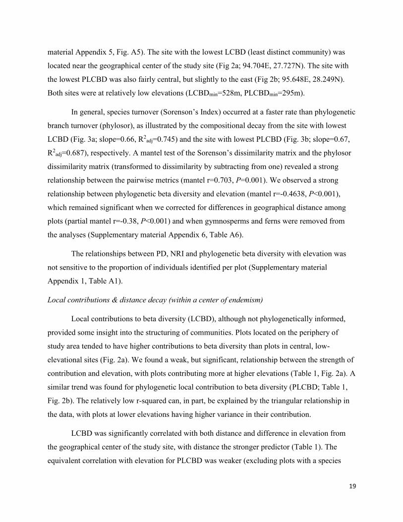
material Appendix 5, Fig. A5). The site with the lowest LCBD (least distinct community) was
located near the geographical center of the study site (Fig 2a; 94.704E, 27.727N). The site with
the lowest PLCBD was also fairly central, but slightly to the east (Fig 2b; 95.648E, 28.249N).
Both sites were at relatively low elevations (LCBDmin=528m, PLCBDmin=295m).
In general, species turnover (Sorenson’s Index) occurred at a faster rate than phylogenetic
branch turnover (phylosor), as illustrated by the compositional decay from the site with lowest
LCBD (Fig. 3a; slope=0.66, R2adj=0.745) and the site with lowest PLCBD (Fig. 3b; slope=0.67,
R2adj=0.687), respectively. A mantel test of the Sorenson’s dissimilarity matrix and the phylosor
dissimilarity matrix (transformed to dissimilarity by subtracting from one) revealed a strong
relationship between the pairwise metrics (mantel r=0.703, P=0.001). We observed a strong
relationship between phylogenetic beta diversity and elevation (mantel r=-0.4638, P<0.001),
which remained significant when we corrected for differences in geographical distance among
plots (partial mantel r=-0.38, P<0.001) and when gymnosperms and ferns were removed from
the analyses (Supplementary material Appendix 6, Table A6).
The relationships between PD, NRI and phylogenetic beta diversity with elevation was
not sensitive to the proportion of individuals identified per plot (Supplementary material
Appendix 1, Table A1).
Local contributions & distance decay (within a center of endemism)
Local contributions to beta diversity (LCBD), although not phylogenetically informed,
provided some insight into the structuring of communities. Plots located on the periphery of
study area tended to have higher contributions to beta diversity than plots in central, low-
elevational sites (Fig. 2a). We found a weak, but significant, relationship between the strength of
contribution and elevation, with plots contributing more at higher elevations (Table 1, Fig. 2a). A
similar trend was found for phylogenetic local contribution to beta diversity (PLCBD; Table 1,
Fig. 2b). The relatively low r-squared can, in part, be explained by the triangular relationship in
the data, with plots at lower elevations having higher variance in their contribution.
LCBD was significantly correlated with both distance and difference in elevation from
the geographical center of the study site, with distance the stronger predictor (Table 1). The
equivalent correlation with elevation for PLCBD was weaker (excluding plots with a species

20
richness of one), and in contrast to results with LCBD, elevation was the better predictor (Table
1). The taxa which contributed the most to beta diversity, as indexed by the species contribution
to beta diversity (SCBD; Legendre and De Caceres 2013), were Castanopsis indica, Duabanga
grandiflora, Pinus roxburghii, and Quercus sp.; these taxa are restricted in their distribution but
have high local abundances. The distribution of both LCBD and PLCBD was qualitatively
similar when gymnosperms and ferns were removed from the analyses (Spearmann rank
correlations; LCBD=0.939, PLCBD=0.853).
Discussion
We explored shifts in tree community structure and richness across one of the largest elevation
gradients in the world, the Himalayas of Arunachal Pradesh, India. We found that species
richness and phylogenetic diversity declined with elevation, a result that is consistent with our
predictions and existing ecological theory. In general, elevational declines in richness are
hypothesized to be due to factors similar to those driving the decline observed along the
latitudinal gradient, such as the reduced availability of resources, colder temperatures and
increased extinction rates at regional scales (Lomolino 2001, McCain and Grytnes 2010). A
reduction of resources (lush soils and nutrients, for example) and colder temperatures at high
elevations can limit the number of individuals and select for species with specific niche attributes
(McCain and Grytnes 2010), with only those species possessing the appropriate traits and
adaptations able to establish and thrive in these environments.
Several lines of evidence in our study suggest that environmental filtering is contributing
to shifts in community structure with elevation; including high local endemism and rapid
phylogenetic turnover that was more strongly tied to changes in elevation than with distance.
However, one key metric used to infer filtering, the net-relatedness index, which describes the
phylogenetic dispersion of lineages (Webb et al. 2002), did not reveal a strong pattern with
elevation. We suggest two possible explanations for the lack of pronounced community
phylogenetic structuring along the elevational gradient despite strong species filtering. First,
important traits could demonstrate convergent evolution, such that distant relatives share similar
ecological habitats. Second, in high montane regions, filtering may operate on evolutionary
distinct glacial relicts, remnants of once more diverse cold-adapted clades. Much previous work
has focused on the former (Jobbágy and Jackson 2000, Kraft et al. 2007 (simulations), Losos
21
2011, Read et al. 2014); here we explore the latter, and consider the phylogenetic evidence for
glacial relicts structuring communities in the high elevations of the Himalayas.
Areas of high topographic relief such as mountain ranges have been linked to the
presence of glacial refugia (Weber et al. 2014) because they provide cooler, more stable climates
during warming periods (Stewart et al. 2010). These refugia provide suitable conditions for
species that have retreated to microclimates resembling those of the last glacial maxima (Vetaas
and Grytnes 2002, Ohlemüller et al. 2008). Such refugia might be increasingly important for
many species given current warming trends (Opgenoorth et al. 2010). However, relict
communities or species are a challenge to identify, usually requiring detailed population genetics
on a regional scale, allowing past patterns of migration to be reconstructed (Hampe et al. 2003,
Petit et al. 2005, Vargas 2007).
Our approach combines knowledge on the evolutionary relationships among species with
information on shifts in community composition and allows us to identify diversity patterns that
might reflect the distribution of relict lineages and glacial refugia. For example, glacial relicts
could represent survivors from once more diverse clades, perhaps a result of higher extinction
rates of related species (Cain 1944, Fryxell 1962, Brooks and Bandoni 1988). Therefore, the
communities in which they are found may be more phylogenetically diverse relative to their
species richness. Because glacial relicts also tend to be range restricted (Habel and Assmann
2009) we expect that relicts would also contribute more to the overall beta diversity of a region.
Although we did not find strong evidence for higher phylogenetic diversity within higher
elevation plots in Arunachal Pradesh, likely because both richness and phylogenetic diversity
tend to decrease with elevation, we show high species and phylogenetic turnover, supporting
evidence for high local endemism in the region.
Investigating phylogenetic beta diversity in addition to species beta diversity provides
added information on evolutionary history and corrects for species non-independence (Graham
and Fine 2008). We found that species turnover occurred at a faster rate than branch turnover
throughout the landscape; this pattern and the strong relationship between the two indices would
be expected under null expectations. Previous work has interpreted higher species turnover as
evidence for niche conservatism plus environmental filtering (Jin et al. 2015). However,
phylogenetic clustering among species should also be expected with high conservatism and

22
strong filtering, which we did not observe. We therefore more carefully explored patterns of
phylogenetic beta diversity, investigating the relative rates of turnover in branches with space
versus elevation (our proxy for environment).
Our results demonstrate that turnover of clade membership occurs along the elevational
gradient, independently from turnover occurring with geographical distance, echoing the findings
of Gonzalez-Caro et al. (2013), which showed that beta diversity in a tropical mountain system
was not related to distance, but to temperature which varies with elevation (McCain and Grytnes
2010). We suggest that general high phylogenetic beta diversity, the strong correlation between
phylogenetic beta diversity and elevation, as well as the lack of clear patterns of species
relatedness indicates environmental filtering of small ranged, evolutionary distinct, taxa. We
propose that these taxa might represent glacial relicts or refuge species.
The presence of glacial relicts would not only disrupt patterns of phylogenetic clustering
predicted at high elevations in strongly filtered communities, but also contribute to the
uniqueness or beta diversity of those communities. We show that high elevation plots do indeed
contribute disproportionately to regional beta diversity. Because highly contributing plots
represent those that contain communities with relatively greater species uniqueness (Legendre
and De Cáceres 2013), they might also reflect the presence of narrow ranged and evolutionarily
distinct endemics. Species with high individual contributions, many of which are endemic to the
region, include Pinus roxburghii (Puri et al. 2011, IUCN RedList 2015), Pinus wallichiana
(Saqib et al. 2013, IUCN RedList 2015) and Livistona jenkinsiana (Sikarwar et al. 2000). Both
environment and distance from the center of the study site were important predictors of
contributions to species beta diversity, indicating that communities are increasingly unique
across space and elevation. In contrast, phylogenetic contributions to beta diversity increased
more strongly with elevation than with distance, indicating that high elevation plots represent
more phylogenetically unique clades. We suggest that the weaker relationship between distance
and phylogenetic contributions to beta diversity might indicate that dispersal limitation may be
less important in our study system. While dispersal limitation has been shown to stabilize centers
of endemism (Weber et al. 2014), it does not appear to have a significant effect on local tree
community structure in Arunachal Pradesh, despite the high proportion of endemics in the
region.

23
Given strong filtering, high elevation taxa are likely well adapted to the environmental
conditions where they are found; some of these species may have retreated to higher, colder,
altitudes following the last glacial maximum. The absence of strong signal in phylogenetic
clustering indicates that these taxa do not, however, represent radiations within one or a few
clades, instead they may represent remnants from formerly more diverse clades in the region.
A better understanding of richness patterns ultimately requires researchers to collect data
in isolated, overlooked, and hard to access regions around the world. We suggest that regions
with unique species, high endemicity and distinct geography should become priorities for
research and conservation. By understanding the historical factors that have shaped them, these
communities might provide insights into responses to future environmental change, not at the
individual species level, but at the level of the ecological assemblage. Through the use of
community-level diversity indices, we showed that filtering strongly drives community structure
across elevations, and we suggest that some high-elevation communities may represent refugia
for glacial relicts. High altitude refugia may be important conservation targets because they can
provide an escape from generally increasing temperatures globally by matching to the cooler
climates resembling the conditions under which many taxa may have evolved.

24
PART III: Conclusions and Future Research
The field of community phylogenetics has grown rapidly in a short time. Phylogenetic methods
not only provide insight into the potential biotic and abiotic processes structuring communities
but also allow us to account for the relatedness (and non-independence) of species. Species
richness patterns provide only limited insight into the multitude of factors that structure
biodiversity patterns. Using phylogeny we can infer process from pattern by factoring
evolutionary history into analyses of diversity and dispersion. Here I explored multiple diversity
metrics that capture information on both richness and phylogenetic composition to investigate
the community assembly of forest trees in the Himalayas of Arunachal Pradesh, India.
Revisiting objectives
The forests of Arunachal Pradesh are species rich and diverse, changing notably across the
landscape. Although many studies on species diversity have been conducted in the region,
community-level diversity patterns have been largely overlooked, perhaps due to the challenges
in sampling species rich regions with difficult terrain. The researchers at NERIST have been able
to provide a detailed, high resolution dataset with which more specific questions of diversity and
richness patterns can be addressed. We find that species richness and phylogenetic diversity
decreased with elevation, but that species relatedness did not vary strongly. The decrease in
species richness with elevation and latitude is well documented in the literature; however,
community-level patterns and trends in phylogenetic structure are less well understood.
Nevertheless, this information is useful in the context of conservation and restoration (more on
this below) and for improving our understanding of the mechanisms structuring species richness
gradients, especially within remote, poorly studied, regions where we lack detailed knowledge of
species ecologies.
We have suggested that environmental filtering plays an important role in structuring
forest communities along the vast elevational gradient in Arunachal Pradesh. Although this
conclusion may not seem surprising, the patterns reported in the literature are not always
consistent with prior expectations. For instance, environmental filtering may occur without

25
leading to a clear pattern of phylogenetic structuring, and no one metric can definitively
conclude process from pattern. We drew inference by combining results on taxonomic and
phylogenetic diversity and turnover (beta diversity), as well as plot level contributions to beta
diversity. We found that phylogenetic beta diversity among plots varied more strongly with
elevation than distance, but that species turnover more quickly than branches. In addition, plots
that contributed more to the overall beta diversity of the region tended to be those furthest from
the center of the study site. Together these patterns suggest that habitat heterogeneity might drive
rapid turnover in species and branches, and that unique species communities are maintained at
higher elevations. Our results provide strong evidence for environmental filtering, even though
we did not detect significant trends in phylogenetic clustering.
By integrating new metrics with phylogeny, we were able to reveal that plots at higher
elevations contribute more to both species and phylogenetic beta diversity. These sites contain
species or lineages that are high in abundance but have restricted distributions. We suggest that
these plots may represent high elevation refugia, or areas where cold-adapted species can persist.
The presence of these evolutionarily distinct taxa in higher elevational sites may also be part of
the explanation for why we do not find strong evidence for phylogenetic clustering at high
elevations.
Our findings have important implications for conservation prioritization in light of
changing climates and increased anthropogenic pressures globally. Anthropogenic pressures in
Arunachal Pradesh are high and projected to increase, as the forests provide several ecosystem
services (timber, food, medicine) to the local communities (Menon et al. 2001). As a result,
deforestation is commonplace and impacts may be particularly severe where the forest is easily
accessed from towns and roads. With rising global temperatures, tree species will be exposed to
additional stresses. For example, recent studies have shown that species are migrating northward
or upwards to remain within their optimal niche envelope (Lenoir et al. 2008, Morueta-Holme et
al. 2015). The impact of both anthropogenic pressures and changing climates is not clear at the
community level. Our study suggests that forest community composition is strongly structured
by the environment. Environmental change is thus likely to impact forest communities. These
changes may, in turn, impact the resources that forests provide to local inhabitants.

26
Phylogenetic diversity may be a useful metric for conservation prioritization because it
can help identify lineages and communities that contain the most functional diversity. Thus,
identifying taxonomically and phylogenetically distinct communities can help inform
conservation prioritization. We have shown that phylogenetically distinct communities are
located at high elevations, and are thus less likely to be exploited by local habitants, but they
may be subject to higher stress from climate change. If species alter their ranges to adjust for
warming temperatures, these cool, high elevation sites might provide important refugia for
temperature-sensitive species.
Future Research
Future work could incorporate species distribution modelling to characterize the climate
niches of high elevation species. With these models, species ranges could be mapped and
overlapped to identify potential barriers to dispersal, and sites with rare or contracting
environments. High resolution environmental data such as humidity, rainfall, temperature and
soil composition will be essential for generating such models, but are often lacking at the
appropriate scale for this region, where very large changes in elevation, slope and aspect can
result in very different environmental regimes over short spatial distances.
We should additionally strive to collect additional data on species’ functional traits.
Although one of the benefits of phylogenetics is the ease with which it can be incorporated into
studies lacking trait data, the various phylogenetic metrics can be improved with additional
functional trait information. Collecting trait information is time consuming and difficult work,
especially for a study of this size, but could provide additional insight into community
structuring. For example, with detailed trait information, it would be possible to test for
convergent evolution and to more directly evaluate evidence for trait dispersion. While
phylogeny might provide a useful proxy for expected ecological similarity among species,
detailed trait data is critical for identifying the specific selective forces structuring species
distributions and co-existence.
With an increased need for richness and conservation assessment throughout the world,
phylogenetic community ecology can provide an additional perspective on how (and sometimes
why) communities are presently structured, as well as how they might adapt to projected
environmental change. Fortunately, the tools required to build phylogenies and to compute

27
phylogenetic metrics are becoming easier to use and more widely available. Trait and species
richness information can complement phylogenetic approaches—but neither approach may be
sufficient on its own. While phylogenetic methods are constrained by various assumptions, they
can begin to account for species non-independence and evolutionary history in analyses of
diversity patterns, and, as I have shown here, potentially identify regions for conservation based
on unique phylogenetic structure. The work presented in this thesis indicates that Arunachal
Pradesh contains phylogenetically unique forests that potentially have a high conservation value,
both in terms of genetic diversity and resource availability for local human populations.

28
Figures
Figure 1: Map of the study site in Arunachal Pradesh, India, with darker shading indicating
higher elevations. The sites in our study range in elevation from 87m to 4090m above sea level.
The geographic center of the study is identified with an arrow in the inset figure (94.704E,
27.727N, elevation: 709m).

29
Figure 2: Maps show the spatial distribution of LCBD (a) and PLCBD (b). For (a) and (b),
symbols are shaded by contribution, where red indicates higher contributions to beta diversity.
The plots with the lowest contributions are colored white and identified with arrows. These plots
represent the least unique sites for LCBD (a) and PLCBD (b), respectively. We also show the
change in local contribution to beta diversity (LCBD; Fig. 2c) and local contribution to
phylogenetic beta diversity (PLCBD; Fig. 2d) of each plot with increasing distance from the
geographical center of the study site (see Fig. 1). Here, symbols are shaded by elevational
differences, where red indicates a large difference in elevation from the center of the site and
blue indicates small differences.

30
Figure 3: The relationship between phylogenetic beta diversity and Sorenson’s beta diversity
from the site with lowest LCBD (a) and the site with lowest PLCBD (b). Both phylogenetic and
Sorenson’s beta diversity are represented on a scale from 0 to 1, where 0 indicates sites that are
compositionally identical and 1 indicates no overlap between sites in either phylogenetic branch
lengths or taxa, respectively.

31
Tables
Table 1: Linear models testing change in LCBD and PLCBD with elevation and distance.
Distance represents the geographical distance between each plot and the geographical center of
the study site while elevation is the absolute value of the difference in elevation between each
plot and the center of the study site (709m).
Model R2adjusted Pmodel Pdistance Pelevation
LCBD
Elevation 0.276 <0.001
Distance + elevation 0.4307 <0.001 <0.001 <0.001
PLCBD
Elevation 0.1628 <0.001
Distance + elevation 0.1666 <0.001 0.456 <0.001

32
References
Baishya, A. 1999. Plant Diversity in Arunachal Pradesh: An Overview. - Proc. Natl. Work.
Environ. Plan. Sustain. Dev. Oppurtunities Challenges Arunachal Pradesh: 16–18.
Behera, M. D. and Kushwaha, S. P. S. 2007. An analysis of altitudinal behavior of tree species in
Subansiri district, Eastern Himalaya. - Biodivers. Conserv. 16: 1851–1865.
Behera, M. et al. 2002. High plant endemism in an Indian hotspot–eastern Himalaya. - Biodivers.
Conserv. 11: 669–682.
Bininda-Emonds, O. R. P. et al. 2007. The delayed rise of present-day mammals. - Nature 446:
507–512.
Birks, H. J. B. and Willis, K. J. 2008. Alpines, trees, and refugia in Europe. - Plant Ecol. Divers.
1: 147–160.
Bremer, B. et al. 2009. An update of the Angiosperm Phylogeny Group classification for the
orders and families of flowering plants: APG III. - Bot. J. Linn. Soc. 161: 105–121.
Brooks, D. and Bandoni, S. 1988. Coevolution and relicts. - Syst. Biol. 37: 19–32.
Bryant, J. A. et al. 2008. Microbes on mountainsides: contrasting elevational patterns of bacterial
and plant diversity. - Proc. Natl. Acad. Sci. U. S. A. 105: 11505–11511.
Butterfield, B. J. and Callaway, R. M. 2013. A functional comparative approach to facilitation
and its context dependence. - Funct. Ecol. 27: 907–917.
Cain, S. 1944. Foundations of plant geography. - Harper & Brothers Publishers.
Callaway, R. M. et al. 2002. Positive interactions among alpine plants increase with stress. -
Nature 417: 844–848.
Cavender-Bares, J. et al. 2004. Phylogenetic overdispersion in Floridian oak communities. - Am.
Nat. 163: 823–843.

33
Chesson, P. 2000. Mechanisms of maintenance of species diversity. - Annu. Rev. Ecol. Syst.:
343–366.
Clarke, J. et al. 2011. Establishing a time-scale for plant evolution. - New Phytol. 192: 266–301.
Cody, M. L. and Diamond, J. M. 1975. Assembly of species communities. - In: Ecology and
evolution of communities. Harvard University Press, pp. 342–444.
Connor, E. and Simberloff, D. 1979. The assembly of species communities: chance or
competition? - Ecology 60: 1132–1140.
Crisp, M. D. and Cook, L. G. 2012. Phylogenetic niche conservatism: what are the underlying
evolutionary and ecological causes? - New Phytol. 196: 681–694.
Currie, D. J. 1991. Energy and large-scale patterns of animal- and plant- species richness. - Am.
Nat. 137: 27–49.
Darwin, C. 1859. On the origins of species by means of natural selection. - London: Murray.
Davies, T. J. and Buckley, L. B. 2012. Exploring the phylogenetic history of mammal species
richness. - Glob. Ecol. Biogeogr. 21: 1096–1105.
Davies, T. J. et al. 2004. Environmental energy and evolutionary rates in flowering plants. - Proc.
Biol. Sci. 271: 2195–2200.
Elton, C. 1946. Competition and the structure of ecological communities. - J. Anim. Ecol.: 54–
68.
Faith, D. 1992. Conservation evaluation and phylogenetic diversity. - Biol. Conserv. 61: 1–10.
Farrell, M. J. et al. 2015. The path to host extinction can lead to loss of generalist parasites. - J.
Anim. Ecol. 84: 978–984.
Forest, F. et al. 2007. Preserving the evolutionary potential of floras in biodiversity hotspots. -
Nature 445: 757–760.

34
Fryxell, P. A. 1962. The relict species concept. - Acta Biotheor. 15: 105–118.
Givnish, T. J. 1999. On the causes of gradients in tropical tree diversity. - J. Ecol. 87: 193–210.
Godoy, O. et al. 2014. Phylogenetic relatedness and the determinants of competitive outcomes. -
Ecol. Lett. 17: 836–844.
Gonzalez-Caro, S. et al. 2014. Phylogenetic alpha and beta diversity in tropical tree assemblages
along regional-scale environmental gradients in northwest South America. - J. Plant Ecol. 7:
145–153.
Gotelli, N. J. 2000. Null model analysis of species co-occurrence patterns. - Ecology 81: 2606–
2621.
Gotelli, N. and Graves, G. 1996. Null models in ecology. - Smithsonian Institution Press.
Graham, C. H. and Fine, P. V. A. 2008. Phylogenetic beta diversity: linking ecological and
evolutionary processes across space in time. - Ecol. Lett. 11: 1265–1277.
Graham, C. H. et al. 2009. Phylogenetic structure in tropical hummingbird communities. - Proc.
Natl. Acad. Sci. U. S. A. 106 Suppl: 19673–19678.
Habel, J. and Assmann, T. 2009. Relict Species: Phylogeography and Conservation Biology (JC
Habel and T Assmann, Eds.). - Springer Science & Business Media.
Hajra, P. et al. 1996. Materials for the flora of Arunachal Pradesh. - Botanical Survey of India.
Hall, T. 1999. BioEdit: a user-friendly biological sequence alignment editor and analysis
program for Windows 95/98/NT. - Nucleic Acids Symp. Ser. 41: 95–98.
Hampe, A. et al. 2003. Rangewide phylogeography of a bird-dispersed Eurasian shrub:
contrasting Mediterranean and temperate glacial refugia. - Mol. Ecol. 12: 3415–3426.
Hawkins, B. A. et al. 2003. Productivity and history as predictors of the latitudinal diversity
gradient of terrestrial birds. - Ecology 84: 1608–1623.

35
Hinchliff, C. E. et al. 2015. Synthesis of phylogeny and taxonomy into a comprehensive tree of
life. - Proc. Natl. Acad. Sci. 112: 12764-12769.
Hollingsworth, P. M. et al. 2009. A DNA barcode for land plants. - Proc. Natl. Acad. Sci. U. S.
A. 106: 12794–12947.
Hooghiemstra, H. and van der Hammen, T. 1998. Neogene and Quaternary development of the
neotropical rain forest: the forest refugia hypothesis, and a literature overview. - Earth-
Science Rev. 44: 147–183.
IUCN 2015. IUCN Red List of Threatened Species. Version 2014.2. <www.iucnredlist.org>.
Jetz, W. et al. 2012. The global diversity of birds in space and time. - Nature 491: 444–448.
Jin, L. S. et al. 2015. Phylogenetic turnover patterns consistent with niche conservatism in
montane plant species. - J. Ecol. 103: 742–749.
Jobbágy, E. and Jackson, R. 2000. Global controls of forest line elevation in the northern and
southern hemispheres. - Glob. Ecol. Biogeogr. 9: 253–268.
Katoh, K. and Standley, D. M. 2013. MAFFT multiple sequence alignment software version 7:
improvements in performance and usability. - Mol. Biol. Evol. 30: 772–780.
Kembel, S. et al. 2010. Picante: R tools for integrating phylogenies and ecology. -
Bioinformatics 26: 1463–1464.
Kerkhoff, A. J. et al. 2014. The latitudinal species richness gradient in New World woody
angiosperms is consistent with the tropical conservatism hypothesis. - Proc. Natl. Acad. Sci.
U. S. A. 111: 8125–8130.
Kraft, N. J. B. et al. 2007. Trait evolution, community assembly, and the phylogenetic structure
of ecological communities. - Am. Nat. 170: 271–83.
Kraft, N. J. B. et al. 2015. Community assembly, coexistence, and the environmental filtering
metaphor. - Funct. Ecol. 29: 592–599.

36
Kress, W. J. et al. 2005. Use of DNA barcodes to identify flowering plants. - Proc. Natl. Acad.
Sci. U. S. A. 102: 8369–8374.
Legendre, P. and De Cáceres, M. 2013. Beta diversity as the variance of community data:
dissimilarity coefficients and partitioning. - Ecol. Lett. 16: 951–963.
Lenoir, J. et al. 2008. A significant upward shift in plant species optimum elevation during the
20th century. - Science 320: 1768–71.
Letcher, S. G. 2010. Phylogenetic structure of angiosperm communities during tropical forest
succession. - Proc. Biol. Sci. 277: 97–104.
Letten, A. D. and Cornwell, W. K. 2015. Trees, branches and (square) roots: why evolutionary
relatedness is not linearly related to functional distance. - Methods Ecol. Evol. 6: 439–444.
Lomolino, M. 2001. Elevation gradients of species-density: historical and prospective views. -
Glob. Ecol. Biogeogr. 10: 3–13.
Losos, J. B. 2008. Phylogenetic niche conservatism, phylogenetic signal and the relationship
between phylogenetic relatedness and ecological similarity among species. - Ecol. Lett. 11:
995–1003.
Losos, J. B. 2011. Convergence, adaptation, and constraint. - Evolution 65: 1827–1840.
Machac, A. et al. 2011. Elevational gradients in phylogenetic structure of ant communities reveal
the interplay of biotic and abiotic constraints on diversity. - Ecography. 34: 364–371.
Magallón, S. et al. 2015. A metacalibrated time-tree documents the early rise of flowering plant
phylogenetic diversity. - New Phytol. 207: 437–453.
Mayfield, M. M. and Levine, J. M. 2010. Opposing effects of competitive exclusion on the
phylogenetic structure of communities. - Ecol. Lett. 13: 1085–1093.
Mayle, F. E. 2004. Assessment of the Neotropical dry forest refugia hypothesis in the light of
palaeoecological data and vegetation model simulations. - J. Quat. Sci. 19: 713–720.

37
McCain, C. and Grytnes, J. 2010. Elevational gradients in species richness. – eLS.
Menon, S. et al. 2001. Identifying Conservation-Priority Areas in the Tropics: a Land-Use
Change Modeling Approach. - Conserv. Biol. 15: 501–512.
Mittelbach, G. G. et al. 2007. Evolution and the latitudinal diversity gradient: speciation,
extinction and biogeography. - Ecol. Lett. 10: 315–331.
Morueta-Holme, N. et al. 2015. Strong upslope shifts in Chimborazo’s vegetation over two
centuries since Humboldt. - Proc. Natl. Acad. Sci. U. S. A. 112: 12741–12745.
Myers, N. 1988. Threatened biotas: “Hot spots” in tropical forests. - Environmentalist 8: 187–
208.
Ndiribe, C. et al. 2013. Phylogenetic plant community structure along elevation is lineage
specific. - Ecol. Evol. 3: 4925–4939.
Ohlemüller, R. et al. 2008. The coincidence of climatic and species rarity: high risk to small-
range species from climate change. - Biol. Lett. 4: 568–572.
Oksanen, J. et al. 2007. The vegan package. - Community Ecol. Packag.: 631–637.
Opgenoorth, L. et al. 2010. Tree endurance on the Tibetan Plateau marks the world’s highest
known tree line of the Last Glacial Maximum. - New Phytol. 185: 332–342.
Parker, I. M. et al. 2015. Phylogenetic structure and host abundance drive disease pressure in
communities. - Nature 520: 542–544.
Pearse, W. D. and Purvis, A. 2013. phyloGenerator: an automated phylogeny generation tool for
ecologists. - Methods Ecol. Evol. 4: 692–698.
Petit, R. et al. 2005. Climate changes and tree phylogeography in the Mediterranean. - Taxon 54:
877–885.
38
Pigot, A. L. and Etienne, R. S. 2015. A new dynamic null model for phylogenetic community
structure. - Ecol. Lett. 18: 153–163.
Procheş, S. et al. 2006. How much evolutionary history in a 10 x 10 m plot? - Proc. Biol. Sci.
273: 1143–1148.
Provan, J. and Bennett, K. D. 2008. Phylogeographic insights into cryptic glacial refugia. -
Trends Ecol. Evol. 23: 564–571.
Puri, A. et al. 2011. Antidyslipidemic and antioxidant activity of Pinus roxburghii needles. -
Med. Chem. Res. 20: 1589–1593.
R Core Team 2015. R: A language and environment for statistical computing. Vienna, Austria;
2014. - URL http//www.R-project.org
Rahbek, C. 1995. The elevational gradient of species richness: a uniform pattern? - Ecography.
18: 200–205.
Read, Q. D. et al. 2014. Convergent effects of elevation on functional leaf traits within and
among species. - Funct. Ecol. 28: 37–45.
Revell, L. 2012. phytools: an R package for phylogenetic comparative biology (and other
things). - Methods Ecol. Evol. 3: 217–223.
Ronquist, F. and Huelsenbeck, J. 2003. MrBayes 3: Bayesian phylogenetic inference under
mixed models. - Bioinformatics 19: 1572–1574.
Roy, P. S. and Behera, M. D. 2005. Assessment of biological richness in different altitudinal
zones in the Eastern Himalayas, Arunachal Pradesh, India. - Curr. Sci. 88: 250–257.
Saqib, A. et al. 2013. Arsenic bioremediation by low cost materials derived from Blue Pine
(Pinus wallichiana) and Walnut (Juglans regia). - Ecol. Eng. 51: 88–94.

39
Schliep, K. 2011. phangorn: Phylogenetic analysis in R. - Bioinformatics 27: 592–293.
Schweiger, O. et al. 2008. A comparative test of phylogenetic diversity indices. - Oecologia 157:
485–495.
Shooner, S. et al. 2015. The phylogenetics of succession can guide restoration: an example from
abandoned mine sites in the subarctic. - J. Appl. Ecol.: in press.
Sikarwar, R. L. S. and Dasila, L. 2000. Livistona jenkinsiana Griff. (Arecaceae) - An endemic
and endangered palm of North East India. - J. Econ. Taxon. Bot. 31: 414–416.
Stebbins, L. G. 1974. Flowering plants: evolution above the species level. - Belknap Press.
Stevens, G. C. 1989. The Latitudinal Gradient in Geographical Range: How so Many Species
Coexist in the Tropics. - Am. Nat. 133: 240–256.
Stevens, G. C. 1992. The Elevational Gradient in Altitudinal Range: An Extension of Rapoport’s
Latitudinal Rule to Altitude. - Am. Nat. 140: 893–911.
Stewart, J. R. et al. 2010. Refugia revisited: individualistic responses of species in space and
time. - Proc. Biol. Sci. 277: 661–671.
Tribsch, A. and Schönswetter, P. 2003. Patterns of endemism and comparative phylogeography
confirm palaeoenvironmental evidence for Pleistocene refugia in the Eastern Alps. - Taxon
52: 477–497.
Vaidya, G. et al. 2011. SequenceMatrix: concatenation software for the fast assembly of multi-
gene datasets with character set and codon information. - Cladistics 27: 171–180.
Valiente-Banuet, A. and Verdú, M. 2007. Facilitation can increase the phylogenetic diversity of
plant communities. - Ecol. Lett. 10: 1029–1036.
Vamosi, S. M. et al. 2009. Emerging patterns in the comparative analysis of phylogenetic
community structure. - Mol. Ecol. 18: 572–592.

40
Vargas, P. 2007. Are Macaronesian islands refugia of relict plant lineages?: a molecular survey. -
Springer Netherlands.
Verdú, M. et al. 2009. Phylogenetic signatures of facilitation and competition in successional
communities. - J. Ecol. 97: 1171–1180.
Vetaas, O. R. and Grytnes, J.-A. 2002. Distribution of vascular plant species richness and
endemic richness along the Himalayan elevation gradient in Nepal. - Glob. Ecol. Biogeogr.
11: 291–301.
Webb, C. 2000. Exploring the Phylogenetic Structure of Ecological Communities: An Example
for Rain Forest Trees. - Am. Nat. 156: 145–155.
Webb, C. O. and Donoghue, M. J. 2005. Phylomatic: tree assembly for applied phylogenetics. -
Mol. Ecol. Notes 5: 181–183.
Webb, C. O. et al. 2002. Phylogenies and Community Ecology. - Annu. Rev. Ecol. Syst. 33:
475–505.
Weber, L. et al. 2014. Patterns of rain forest plant endemism in subtropical Australia relate to
stable mesic refugia and species dispersal limitations. - J. Biogeogr. 41: 222–238.
Whittaker, R. H. 1960. Vegetation of the Siskiyou Mountains, Oregon and California. - Ecol.
Monogr. 30: 279–338.
Wiens, J. and Graham, C. 2005. Niche conservatism: integrating evolution, ecology, and
conservation biology. - Annu. Rev. Ecol. Evol. Syst. 36: 519–539.
Winter, M. et al. 2013. Phylogenetic diversity and nature conservation: where are we? - Trends
Ecol. Evol. 28: 199–204.
Zanne, A. E. et al. 2014. Three keys to the radiation of angiosperms into freezing environments. -
Nature 506: 89–92.

41
Supplementary Material
Appendix 1: Assessing sensitivity of results to differences in species identification among
plots.
Areas of high diversity, although ecologically invaluable, pose a unique challenge for
researchers. Species identification is highly related to the knowledge of the field personnel and
researchers involved (Elliott and Davies 2014). As such, not all individual trees in our study
were identified to the genus level. To determine whether the discrepancy among plots (in terms
of species identification) had any effect on the overall patterns we observed, we separated our
data into three groups: all 291 plots used in the study, plots with at least 50% of individuals
identified to genus level (257 plots), and plots with at least 75% of individuals identified to
genus level (174 plots).
Using the same 100 phylogenies as for all other analyses, we calculated phylogenetic
diversity (PD), the non-abundance weighted net-relatedness index (NRI) and phylogenetic beta
diversity (PBD) for the three groups of plots, defined above. We regressed PD and NRI for each
group with log-transformed elevation and calculated mantel tests for pairwise phylogenetic beta
diversity and pairwise elevation or distance. We found that the patterns we observed in the study
were conserved for all groups, suggesting that using all plots, despite varying levels of species
non-identification does not affect general patterns of phylogenetically informed indices along the
elevational gradient and overall landscape (Table A1). Phylogenetic metrics such as PD, NRI
and PBD are calculated as standardized effect sizes using 1000 null iterations each, which
corrects for differences in species richness (higher richness with elevation) at the plot level.
Moreover, these metrics consider evolutionary information maintained in the branch lengths and
adding or removing taxa (phylogenetic tips) may not add significant evolutionary information or
alter the overall patterns observed.

42
Table A1: Regressions for both PD and NRI against log-transformed elevation for three groups
of plots (all plots, at least 50% identified, at least 75% identified). We also include the results
from mantel tests for distance matrices of phylogenetic beta diversity, elevational differences and
distance.
Linear models
Model R2adj P F DF
PD~elevation
All plots (291) 0.198 <0.001 72.82 289
50% identified (257) 0.198 <0.001 64.31 255
75% identified (174) 0.208 <0.001 46.47 172
NRI~elevation
All plots (291) 0.133 <0.001 44.83 285
50% identified (257) 0.192 <0.001 60.87 251
75% identified (174) 0.251 <0.001 57.56 168
Mantel Test
Model mantel-r P
PBD~elevation (mantel)
All plots (291) -0.4638 0.001
50% identified (257) -0.4767 0.001
75% identified (174) -0.4473 0.001
PBD~distance (mantel)
All plots (291) -0.312 0.001

43
50% identified (257) -0.3412 0.001
75% identified (174) -0.3575 0.001
References
Elliott, T. L. and Davies, T.J. 2014. Challenges to barcoding an entire flora. –Mol. Ecol. Res. 14:
883–891.

44
Appendix 2: Genbank accession numbers for phylogeny reconstruction.
Table A2: List of accession numbers used to reconstruct the 100 phylogenies used in the study.
In some cases, sequences were not available for the species in our study and we used sequences
for closely related species. Both the species names for the sequences and the name used in the
phylogenies are noted.
GenBank species name MATK RBCL ITS1-2 Name in phylogeny
Abies alba HQ619823.1 FR831929.1 Abies alba
Abroma augusta HM488448.1 AJ012208.1 AJ277462.1 Abroma augusta
Acacia catechu AF274141.1 GQ436355.1 KC952019.1 Acacia sp.
Acer caesium DQ978397.1 Acer caesium
Acer campbellii JF952995.1 DQ978398.1 HM352652.1 Acer campbellii
Acer cappadocicum AJ634579.1 Acer cappadocicum
Actinodaphne obovata AF244410.1 AY265398.1 Actinodaphne obovata
Aglaia elaeagnoidea AB925001.1 AB925482.1 AY695536.2 Aglaia spectabilis
Ailanthus integrifolia EU042843.1 JF738642.1 Ailanthus integrifolia
Alangium chinense FJ644642.1 L11209.2 FJ610017.1 Alangium chinense
Albizia lebbeck JX495667.1 KC417043.1 Albizia lebbeck
Albizia lucidior JX856396.1 Albizia lucidior
Albizia procera KC689800.1 KC417044.1 JX856397.1 Albizia procera
Alnus nepalensis JF953073.1 FJ844581.1 AJ251676.1 Alnus nepalensis
Alsophila spinulosa AB574756.1 Cyathea spinulosa
Alstonia scholaris Z70189.1 X91760.1 DQ358880.1 Alstonia scholaris
Altingia excelsa AF013037.1 AJ131769.1 AF304525.1 Altingia excelsa
Angiopteris evecta EU439092.1 Angiopteris evecta
Aquilaria sinensis HQ415244.1 GQ436619.1 KF636364.1 Aquilaria malaccensis
Aralia cachemirica AY725107.1 Aralia sp
Ardisia crenata GU135103.1 GU135270.1 JF416242.1 Ardisia macrocarpa
Artocarpus chama AB924725.1 AB925336.1 FJ917047.1 Artocarpus chama
Artocarpus heterophyllus JX856635.1 FJ917039.1 Artocarpus heterophyllus
Azadirachta indica EF489115.1 AJ402917.1 AY695594.1 Azadirachta indica
Baccaurea lanceolata AY552419.1 Baccaurea ramiflora
Bambusa balcooa JX966236.1 EU244594.1 Bambusa balcooa

45
Bambusa tulda EU434248.1 EF540854.1 Bambusa tulda
Bauhinia ungulata JQ587517.1 JQ591586.1 FJ009818.1 Bauhinia ungulata
Beilschmiedia roxburghiana AB924825.1 AB925437.1 Beilschmiedia fagifolia
Berberis asiatica GU934752.1 GU934836.1 GU934647.1 Berberis leschenaultii
Bhesa robusta AB925166.1 AY935723.1 Bhesa robusta
Bischofia javanica EF135508.1 AY663571.1 Bischofia javanica
Boehmeria glomerulifera KF138115.1 KF137807.1 Boehmeria glomerulifera
Boehmeria macrophylla KF137956.1 JF317496.1 KF835865.1 Boehmeria macrophylla
Boehmeria nivea KF137957.1 AJ235801.1 KF835885.1 Boehmeria nivea
Boehmeria platyphylla KF835876.1 Boehmeria platyphylla
Boehmeria rugulosa KF137960.1 KF138125.1 KF137817.1 Boehmeria rugulosa
Bombax ceiba JX495673.1 JN114787.1 HQ658377.1 Bombax ceiba
Brassaiopsis hispida JQ933245.1 AY725117.1 Brassaiopsis mitis
Breonia chinensis AJ346968.1 AJ346858.1 Breonia chinensis
Bridelia retusa HQ415363.1 FJ439910.1 Bridelia retusa
Brucea javanica AB924837.1 EU042986.1 AY510155.1 Brucea javanica
Calamus erectus JQ041983.1 JQ042035.1 Calamus sp
Callicarpa arborea FM163260.1 JF738395.1 FM163241.1 Callicarpa arborea
Callicarpa macrophylla FM163273.1 JQ618476.1 FM163246.1 Callicarpa macrophylla
Camellia sinensis AF380077.1 AF380037.1 EU579774.1 Camellia sinensis
Canarium strictum FJ466638.1 Canarium strictum
Carallia brachiata AF105086.1 AB925477.1 AF328957.1 Carallia brachiata
Caryota urens JF344998.1 JQ734494.1 JF344933.1 Caryota urens
Casearia glomerata HQ415293.1 Casearia vareca
Cassia fistula JQ301870.1 JX571794.1 JX856432.1 Cassia fistula
Castanopsis indica JF953474.1 JF941185.1 AY040377.1 Castanopsis indica
Casuarina stricta U92858.1 Casuarina sp
Chukrasia tabularis AB924866.1 AB925481.1 FJ518894.1 Chukrasia tabularis
Cinnamomum bejolghota GQ248098.1 GQ248569.1 Cinnamomum bejolghota
Citrus maxima AB626794.1 GQ436734.1 AB673398.1 Citrus maxima
Citrus reticulata FJ716729.1 JQ593913.1 AB456115.1 Citrus reticulata
Clerodendrum infortunatum JQ724863.1 Clerodendrum infortunatum
Cordia africana KF158134.1 Cordia grandis

46
Coriaria nepalensis KF022395.1 KF022461.1 KF022334.1 Coriaria nepalensis
Cornus capitata DQ341340.1 AY530926.1 AY530915.1 Cornus capitata
Cupressus torulosa HM023995.1 AY988257.1 AY988393.1 Cupressus torulosa
Cyathea podophylla JF303907.1 Cyathea sp
Cyathea klossi EU352299.1 Cyathea sp
Dalbergia sissoo AF203582.1 JX571817.1 EF451079.1 Dalbergia sissoo
Daphne laureola HM850899.1 JN892035.1 GQ167536.2 Daphne papyracea
Debregeasia saeneb JF317422.1 JF317481.1 KF137835.1 Debregeasia saeneb
Dendrocalamus hamiltonii HM448942.1 Dendrocalamus hamiltonii
Dillenia indica AB924752.1 FJ860350.1 AY096030.1 Dillenia indica
Dipterocarpus retusus KF021568.1 Dipterocarpus retusus
Docynia indica JQ391000.1 JQ933307.1 JQ392426.1 Docynia indica
Duabanga grandiflora GQ434087.1 AY036150.1 AF163695.1 Duabanga grandiflora
Dysoxylum binectariferum JX982143.1 JX982144.1 JX982145.1 Dysoxylum binectariferum
Elaeagnus umbellata AY257529.1 HM849968.1 AF440257.1 Elaeagnus parvifolia
Elaeocarpus sphaericus AF206765.1 DQ499079.1 Elaeocarpus floribundus
Elatostema acuminatum AY208702.1 Elatostema platyphyllum
Engelhardia fenzelii AY147099.1 AY147095.1 KF201317.1 Engelhardia spicata
Erythrina lanceolata JQ587635.1 JQ591753.1 Erythrina stricta
Eucalyptus tereticornis AF390482.1 Eucalyptus sp.
Eurya acuminata AY626852.1 Eurya acuminata
Eurya japonica AF380081.1 Z80207.1 AY626867.1 Eurya japonica
Exbucklandia populnea U77092.1 AF081071.1 AF127504.1 Exbucklandia populnea
Ficus auriculata JQ773629.1 JQ773648.1 JQ773837.1 Ficus auriculata
Ficus benjamina JQ773507.1 JX571829.1 JQ773842.1 Ficus benjamina var. nuda
Ficus cyrtophylla JF953730.1 JF941526.1 JQ773858.1 Ficus cyrtophylla
Ficus glaberrima JF953733.1 JF941532.1 JQ773885.1 Ficus glaberrima
Ficus hirta HQ415330.1 JQ773693.1 JQ773900.1 Ficus hirta
Ficus hispida KC508602.1 GU935070.1 JQ773905.1 Ficus hispida
Ficus racemosa GU935040.1 JF941550.1 HM368196.1 Ficus racemosa
Ficus semicordata JQ773468.1 JF941553.1 JQ773985.1 Ficus semicordata
Garcinia cowa HQ331596.1 HQ332054.1 AB110799.1 Garcinia cowa
Garcinia pedunculata KF783274.1 Garcinia pedunculata
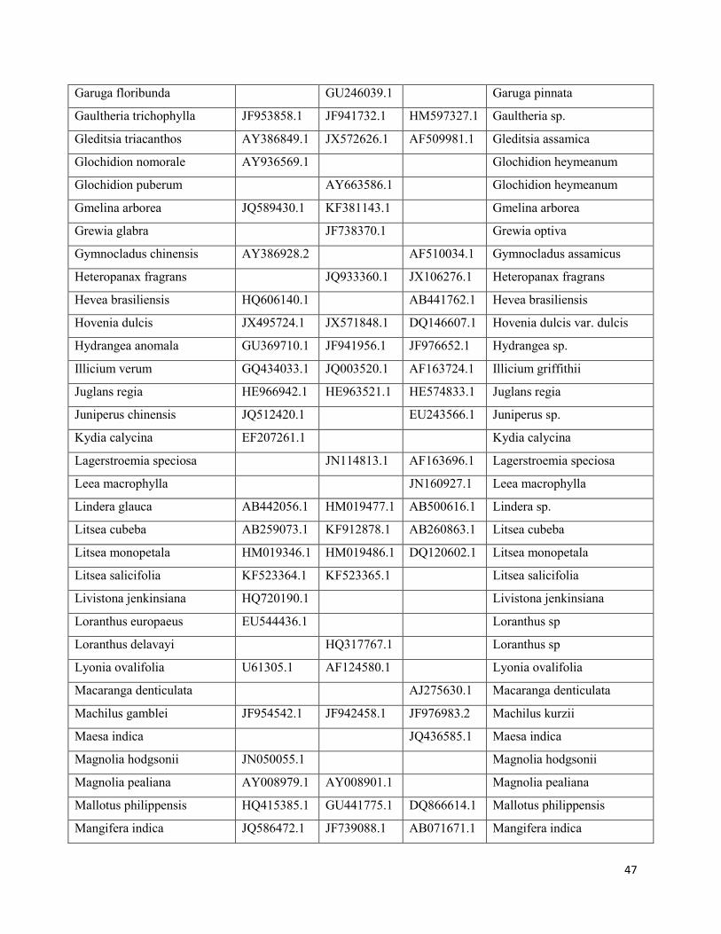
47
Garuga floribunda GU246039.1 Garuga pinnata
Gaultheria trichophylla JF953858.1 JF941732.1 HM597327.1 Gaultheria sp.
Gleditsia triacanthos AY386849.1 JX572626.1 AF509981.1 Gleditsia assamica
Glochidion nomorale AY936569.1 Glochidion heymeanum
Glochidion puberum AY663586.1 Glochidion heymeanum
Gmelina arborea JQ589430.1 KF381143.1 Gmelina arborea
Grewia glabra JF738370.1 Grewia optiva
Gymnocladus chinensis AY386928.2 AF510034.1 Gymnocladus assamicus
Heteropanax fragrans JQ933360.1 JX106276.1 Heteropanax fragrans
Hevea brasiliensis HQ606140.1 AB441762.1 Hevea brasiliensis
Hovenia dulcis JX495724.1 JX571848.1 DQ146607.1 Hovenia dulcis var. dulcis
Hydrangea anomala GU369710.1 JF941956.1 JF976652.1 Hydrangea sp.
Illicium verum GQ434033.1 JQ003520.1 AF163724.1 Illicium griffithii
Juglans regia HE966942.1 HE963521.1 HE574833.1 Juglans regia
Juniperus chinensis JQ512420.1 EU243566.1 Juniperus sp.
Kydia calycina EF207261.1 Kydia calycina
Lagerstroemia speciosa JN114813.1 AF163696.1 Lagerstroemia speciosa
Leea macrophylla JN160927.1 Leea macrophylla
Lindera glauca AB442056.1 HM019477.1 AB500616.1 Lindera sp.
Litsea cubeba AB259073.1 KF912878.1 AB260863.1 Litsea cubeba
Litsea monopetala HM019346.1 HM019486.1 DQ120602.1 Litsea monopetala
Litsea salicifolia KF523364.1 KF523365.1 Litsea salicifolia
Livistona jenkinsiana HQ720190.1 Livistona jenkinsiana
Loranthus europaeus EU544436.1 Loranthus sp
Loranthus delavayi HQ317767.1 Loranthus sp
Lyonia ovalifolia U61305.1 AF124580.1 Lyonia ovalifolia
Macaranga denticulata AJ275630.1 Macaranga denticulata
Machilus gamblei JF954542.1 JF942458.1 JF976983.2 Machilus kurzii
Maesa indica JQ436585.1 Maesa indica
Magnolia hodgsonii JN050055.1 Magnolia hodgsonii
Magnolia pealiana AY008979.1 AY008901.1 Magnolia pealiana
Mallotus philippensis HQ415385.1 GU441775.1 DQ866614.1 Mallotus philippensis
Mangifera indica JQ586472.1 JF739088.1 AB071671.1 Mangifera indica

48
Melastoma malabathricum AF270748.1 GQ265880.1 Melastoma malabathricum
Melia azedarach EF489117.1 JX856725.1 AY695595.1 Melia azedarach
Merrilliopanax listeri KC952369.1 Merrilliopanax alpinus
Mesua ferrea HQ331661.1 GQ436685.1 AY625635.1 Mesua ferrea
Meyna tetraphylla AJ315083.1 Meyna laxiflora
Michelia champaca AY008902.1 Michelia champaca
Micromelum integerrimum JX144208.1 Micromelum integerrimum
Moringa oleifera JX092021.1 JX571866.1 AF378589.1 Moringa oleifera
Morus macroura GU145567.1 GU145581.1 AB604232.1 Morus laevigata
Musa acuminata KC904699.1 FJ871828.1 JF977066.1 Musa sp.
Myrica esculenta FJ469994.1 Myrica esculenta
Oroxylum indicum GQ434292.1 JN407262.1 FJ606747.1 Oroxylum indicum
Ostodes paniculata EF135574.1 AJ402979.1 Ostodes paniculata
Pandanus tectorius JX903664.1 M91632.1 EU816709.1 Pandanus furcatus
Persea bombycina EU128737.1 Persea odoratissima
Phlogacanthus thyrsiflorus EU528907.1 Phlogacanthus thyrsiflorus
Phoebe lanceolata AB924934.1 AB925556.1 FM957844.1 Phoebe cooperiana
Phyllanthus emblica FJ235251.1 AB925416.1 AB550082.1 Phyllanthus emblica
Pieris formosa U61303.2 AF124581.1 EU547690.1 Pieris formosa
Pinus kesiya AB161008.1 JN039276.1 AF037004.1 Pinus kesiya
Pinus merkusii AY497287.1 AB019811.1 AF037006.1 Pinus merkusii
Pinus roxburghii AB084495.1 JN854162.1 AF037021.1 Pinus roxburghii
Pinus wallichiana JN854154.1 X58131.1 AF036991.1 Pinus wallichiana
Podocarpus neriifolius KF713737.1 AF249618.1 KF713961.1 Podocarpus neriifolius
Prunus cerasoides HQ235127.1 HQ235411.1 JQ034160.1 Prunus cerasoides
Psidium guajava JQ588510.1 JQ592981.1 AB354956.1 Psidium guajava
Pterospermum acerifolium KJ510943.1 JX856493.1 Pterospermum acerifolium
Pterospermum lanceifolium AB924689.1 HQ415058.1 JX856596.1 Pterospermum lanceifolium
Pyrus communis JN895841.1 JQ391382.1 JQ392467.1 Pyrus communis
Quercus baloot HE583734.1 HE591363.1 Quercus baloot
Quercus glauca JX860839.1 AB060571.1 HE611290.1 Quercus glauca
Quercus leucotrichophora JX860844.1 Quercus leucotrichophora
Rhododendron arboreum JF955906.1 JF943838.1 JF978202.1 Rhododendron arboreum

49
Rhododendron barbatum EU087304.1 Rhododendron barbatum
Rhododendron cinnabarinum JF943863.1 JF978227.1 Rhododendron cinnabarinum
Rhododendron falconeri U61343.1 Rhododendron falconeri
Rhododendron fulgens EU087314.1 Rhododendron fulgens
Rhododendron grande U61336.1 GU176646.1 GU176633.1 Rhododendron grande
Rhododendron lanatum EU087332.1 Rhododendron lanatum
Rhododendron maddenii JF956017.1 JF943959.1 AY877281.1 Rhododendron maddenii
Rhododendron thomsonii EU087359.1 Rhododendron thomsonii
Rhododendron wallichii JF956143.1 JF944100.1 JF978451.1 Rhododendron wallichii
Rhus chinensis EF682845.1 Rhus chinensis
Ricinus communis GU134993.1 GU135207.1 AY918198.1 Ricinus communis
Sambucus adnata JF956193.1 JF944171.1 JF978510.1 Sambucus adnata
Sarcochlamys pulcherrima KF138244.1 KF137924.1 Sarcochlamys pulcherrima
Saurauia nepaulensis Z83147.1 Saurauia nepaulensis
Schefflera venulosa JF284828.1 Schefflera venulosa
Schima khasiana HM100439.1 Schima khasiana
Schima wallichii AF380100.1 AF380056.1 HM100444.1 Schima wallichii
Senna siamea GU942496.1 JQ301862.1 KC984644.1 Senna siamea
Shorea assamica AB246453.1 Shorea assamica
Shorea robusta JX856763.1 Shorea robusta
Smilax perfoliata JF956459.1 JF944425.1 JF978768.1 Smilax sp.
Spondias mombin AY594480.1 GQ981882.1 AF445882.1 Spondias pinnata
Sterculia apetala GQ982103.1 JQ594218.1 Sterculia villosa
Stereospermum chelonoides KF199892.1 Stereospermum chelonoides
Styrax officinalis AJ429300.1 EU980810.1 AF327489.1 Styrax sp.
Syzygium cumini GU135062.1 FM887016.1 Syzygium cumini
Syzygium jambos DQ088583.1 JQ592986.1 AM234135.1 Syzygium jambos
Tectona grandis FM163282.1 JQ618492.1 FM163255.1 Tectona grandis
Terminalia bellirica AF425714.1 FJ381773.1 Terminalia bellirica
Terminalia chebula AB924845.1 FJ381812.1 FJ381775.1 Terminalia chebula
Terminalia myriocarpa FJ381816.1 FJ381779.1 Terminalia myriocarpa
Tetrameles nudiflora AY968458.1 AF206828.1 AF280105.1 Tetrameles nudiflora
Toona ciliata JX518246.1 FJ462488.1 Toona ciliata

50
Toona sureni KC155954.1 Toona sureni var. sureni
Toxicodendron griffithii FJ945925.1 Toxicodendron griffithii
Trema orientalis JX518199.1 AB925367.1 AY488734.1 Trema orientalis
Trevesia palmata GQ434261.1 U50258.1 KF591488.1 Trevesia palmata
Trewia nudiflora AY663648.1 DQ866628.1 Trewia nudiflora
Tsuga dumosa EF395590.1 AF145460.1 EF395515.1 Tsuga dumosa
Vernonia cinerea GU724239.1 AY142953.1 Vernonia arborea
Viburnum colebrookeanum HQ591570.1 HQ591715.1 HQ591959.1 Viburnum colebrookeanum
Viburnum cylindricum JF956777.1 JF944759.1 JF979002.1 Viburnum cylindricum
Walsura robusta AB924714.1 AB925325.1 Walsura robusta
Wendlandia tinctoria HM119580.1 FM207649.1 FM204699.1 Wendlandia glabrata
Zanthoxylum armatum GQ436751.1 DQ016546.1 Zanthoxylum armatum
Ziziphus mauritiana JX518013.1 JX856806.1 DQ146589.1 Zizyphus mauritiana

51
Appendix 3: Example phylogeny.
Figure A3: One of the 100 phylogenies used in this study. The phylogenies were built for 279
species and rooted on Angiopteris evecta, identified as the most basal species present in our
species pool.

52
Appendix 4: The relationship between the standardized effect size of phylogenetic diversity
and elevation.
Glacial refugia may sustain a disproportionate amount of phylogenetic diversity if relict species
are phylogenetically unique, perhaps due to the local extinction of closely related species. The
standardized effect size of phylogenetic diversity (ses.pd) corrects for species richness and can
provide significance with a null model that compares observed phylogenetic diversity to
simulated phylogenetic diversity, given species richness and the regional phylogeny. We found
that ses.pd increased with log-transformed altitude (R2adj=0.156, P<0.001). This suggests that
plots at high elevations have higher phylogenetic diversity than expected given species richness.
Although we find a trend of increasing ses.pd with elevation, the 39/291 plots with significant
ses.pd were located throughout the region at elevations ranging from 192m to 3863m.
Consequently, there was no relationship between plots with significant PD and elevation
(R2adj=0.002, P=0.299).
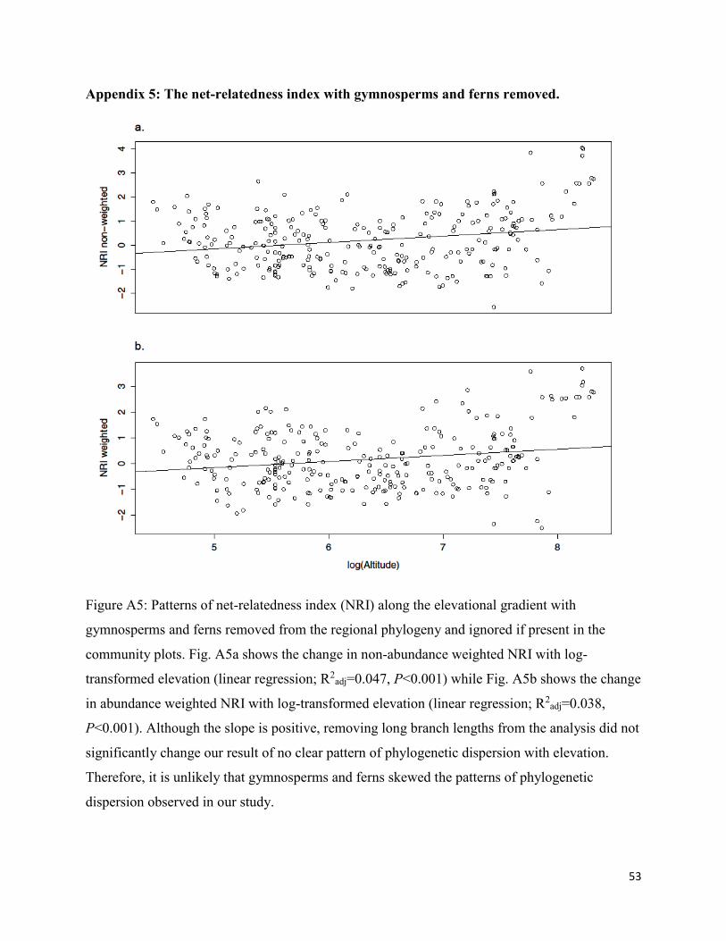
53
Appendix 5: The net-relatedness index with gymnosperms and ferns removed.
Figure A5: Patterns of net-relatedness index (NRI) along the elevational gradient with
gymnosperms and ferns removed from the regional phylogeny and ignored if present in the
community plots. Fig. A5a shows the change in non-abundance weighted NRI with log-
transformed elevation (linear regression; R2adj=0.047, P<0.001) while Fig. A5b shows the change
in abundance weighted NRI with log-transformed elevation (linear regression; R2adj=0.038,
P<0.001). Although the slope is positive, removing long branch lengths from the analysis did not
significantly change our result of no clear pattern of phylogenetic dispersion with elevation.
Therefore, it is unlikely that gymnosperms and ferns skewed the patterns of phylogenetic
dispersion observed in our study.

54
Appendix 6: Mantel tests for phylogenetic beta diversity against elevation and distance
with gymnosperms and ferns removed.
Table A6: Mantel tests were calculated for pairwise phylogenetic beta diversity (PBD; calculated
with phylosor) with gymnosperms and ferns removed against elevation, distance or both. Results
show strong, negative relationships between phylogenetic beta diversity (shared branch lengths)
and elevation, even when correcting for differences in distance, which is consistent with our
results when gymnosperms and ferns were included in the analysis.
Model mantel-r P
PBD~elevation -0.481 <0.001
PBD~distance -0.320 <0.001
PBD~elevation + distance -0.400 <0.001