Community Detection Algorithms: acomparative evaluation on artificial and

real-world networks

D.Phil student report

Department of Engineering Science

Department of Zoology

PSORAKIS IOANNIS

supervisors: Prof Stephen Roberts, Prof Ben SheldonUniversity of Oxford

October 21, 2010

1

Abstract

In this report we provide a brief ‘research diary’ of our work on commu-nity detection. We present an overview of widely adopted algorthms alongwith a comparative analysis against real-world and computer-generated net-works. Most imporantly, among these methods we present a novel proba-bilistic community detection algorithm that provides state of the art resultswith minimal computational overhead.

1 Introduction

The network paradigm provides a formal way of representing data whose associa-tions are of the outmost importance in order to understand the phenomenon understudy. Many systems in nature consist of interconnected entities [1][2]; the be-haviour of each of those entities at an individual level determines (more or lessobviously) the function of the whole system at large scale.

While networks have already been studied in a rigorous mathematical frame-work in previous centuries (from the foundations of Graph Theory in 18th centuryto the combinatorial analysis problems of the 20th century) [1][2][3], modern ad-vances in data storage and manipulation technologies have allowed a massive resur-gence in the study of networks. The plethora of different problems, ranging fromsocial interactions to neuron connectivities lead to an interdisciplinary approach tosuch problems, using tools from Statistical Mechanics and Computer Science toBehavioural Sciences and Sociology [2].

According to Mark Newman, real world networks can be classified into fourcategories [1]; (a)social networks that represent the pattern of interactions betweenindividuals (from human acquaintances to instances of animal behavioural traits),(b) information networks that reflect a knowledge dependency model (for examplethe journal citation network), (c) technological networks that represent the distribu-tion of resources (from the electricity grid to airline routes) and finally (d) biologi-cal networks that capture the structure of systems such as the metabolic pathwaysor protein interactions.

Social networks are a major area of research in the recent years [4]. Human so-cial networks are now an important aspect of people’s everyday interactions and theever-increasing connectivity amongst individuals has lead to a major interest in theform and function of these networks. Additionally, advances in sensor technologyhave facilitated the collection of zoological field data, where animal interactionsare now being observed and evaluated at a larger scale. A major aspect of socialnetwork research is the study of community structure i.e the form and functionof network parts or modules with ‘hot-spots’ of hightened connectivity. Indeed,

2

a significant research effort is invested on the development of methodologies forcommunity detection that consist of:

• evaluating if the given network has a modular, non-random structure.

• identifying the different partitions (groups of individuals) that the networkconsists of.

• evaluating the function and roles of these modules.

In the present work, our intention is to provide a preliminary analysis of socialnetworks and more specifically present an evaluation of different modern commu-nity detection algorithms against real and artificial datasets. Among these models,we also present the performance of a novel probabilistic community detection al-gorithm that provides extremely competitive performance without suffering someimportant weaknesses of the standard approaches.

This report is organized as follows: initially we provide a short description ofGraph Theory notions we will use throughout the report, along with the necessarynotation. Then we discuss the notion of community structure and how to quantifyit in a mathematical sense. Then we provide a brief overview of the communitydetection methodologies we have implemented and used for our experiments alongwith the results for artificial and real world datasets. Based on the outcomes of ourexperiments, we conclude by discussing ideas and challenges for future work.

2 Theoretical Background

In this section we provide an overview of the network theory notions we utilize forour study along with some critical discussion of the basic approaches to commu-nity detection and social network analysis. We start from a purely mathematicallevel describing main notions and notation and proceed by expanding our view tothe interdisciplinary problem of defining assessing the community structure of anetwork. Main ideas such as the modularity are introduced.

2.1 Graph Theory notions and notation

A graph is the abstract representation of a set V of N entities along with theircorresponding M connections D; each individual or node or vertex {ni}Ni=1 ∈ Vis linked to a subset of V via a collection of M edges {li}Mi=1 ∈ D. An examplegraph is shown in Fig 1.

Each graph G = {V,D} can be conveniently represented in the form of anN × N adjacency matrix A where if Aij 6= 0 then i points to j. In the simplest

3

Figure 1: A sample graph with eight vertices and ten edges [1]

of cases, we are only interested in just the presence or absence of a connectionbetween two entities therefore we have an unweighted graph with Aij ∈ {0, 1}.We follow the convention that Aii = 0. In the more general case of a weightednetwork, Aij takes values that reflect the strength with which i is connected to j.If A is symmetric, then we have an undirected graph and vice-versa. For thepurposes of the present work, we are not interested in other graph types such asbipartite graphs, hypergraphs, etc.

For real-world networks, for each pair of nodes the presence of an edge mayrepresent dependence, similarity, direct reachability, commodity flow, causality orany other concept depending on the problem context and modelling assumptions.On the opposite case, where the presence of an edge between any pair of nodes isa random variable P (Aij = 1) = p, then we have an Erdis Renyi random graph.ER random graphs have been studied in detail in the previous years (see [1] foran overview) and are being widely used in order to evaluate the significance ofinferred structures from real-world networks [6][13].

2.2 Network properties

The study of networks typically consists of looking at different scales of the graphin order to make inferences about the form and function of its modules. Thus, wedefine sets of properties of individual vertices of the graph along with propertiesthat characterize the network as a whole [1].

Local properties [5] are defined by the topology of the network in the localneighborhood of a single node. Some of them are the degree of a vertex-i, that isthe number of adjacent vertices, the clustering coefficient that measures the prob-ability that two adjacent vertices of i will also be connected, the node centralitythat measures how many shortest paths in the network pass through that individualvertex, etc. Naturally, in real world networks nodes can have other properties, forexample in an animal social network a node can have features such as age, gender,

4

species etc but these are not been taken into account at least during the first stagesof the analysis.

Global properties [5] are defined from large-scale statistical properties of thenetwork under study. One of the most important properties is the degree distribu-tion; that is the probability that a node-i will have a degree ki. It has been widelyacknowledged that the degree distribution accounts for many of the networks func-tions, such as the way it is structured into communities. For the majority of realworld networks, the degree distribution follows the power-law [2] [5] i.e the per-centage of vertices with degree ki drops exponentially as we increase ki. Otherglobal properties can be the weight distribution for weighted networks, the globalclustering coefficient which is the average of node clustering coefficients, averageshortest path which is the average geodesic distance between any pair of nodesor the degree corelation which is the probability that nodes with degree k will beconnected to nodes with degree k′. The latter characterizes networks as assortative(nodes with same degree tend to be connected) or disassortative (inversely).

Mesoscopic properties. These characteristics lie on a scale between the globaland the local perspective of the network. They describe the community or modularstructure of the network and will be discussed in the following section.

2.3 Community structure in networks

Although the idea that a network can be partitioned into groups that have somequalitative characteristic is very intuitive, it has been widely acknowledged that itcan be quite difficult to formalize it in a mathematical way [3] [2]. That is because,the idea of community (or module or group) itself is not very well defined in acontext-independent way. Nevertheless, according to a common definition in theliterature, community is a subset gc ∈ V of nodes that are more densely connectedto each other than with the rest of the network. Thus, given a single community gcin the network, and based on [13] that is:

2min

n(n− 1)>

2M

N(N − 1)>

mout

n(N − n)(1)

where min is the number of edges connecting nodes belonging to gc, n is thesize (or cardinality) of gc, mout is the number of links connecting a node in gswith another one at the external network. The denominators represent the totalnumber of possible connections between nodes of the same community, the wholenetwork, the nodes outside the community. Equation (1) defines that the proportionof intra-community links is larger than that of the whole network. Additionally, weexpect that the fraction of inter-community links to be lower than the other two.

5

Therefore, community structure in the network consists of ‘hot-spots’ of increasedconnectivity, as seen in Fig. 2.

Figure 2: A sample community structure given a small network [3].

In real-world networks, communities represent modules that have special char-acteristics or play a distinct role in the network [2] [3]; for example in human socialnetworks communities represent cliques of friends, in citation networks representgroups of similar field of research and in transportation networks hubs of high ge-ographical proximity. At this point it is important to state that given a network andbased on its topology and weights we are inferring structural communities, whichmight not always reflect functional ones [2]. I

It is very natural for real world networks to possess a nested or hierarchicalcommunity struture [2][6], i.e each individual community can be further parti-tioned into other subcommunities. Therefore, the whole community structure ofthe network can be represented in the form of a dendogram, see Fig. 3, where thetop node represents the whole graph and each layer below a possible partition. Thecommunity dendogram reflects the community organization of a network underdifferent resolution perspectives.

On the other hand, in random graphs links tend to form between nodes withoutany regard of mesoscopic cohesiveness. Based on that difference betweeen realand random networks, Mark Newman and Michelle Girvan proposed in [6] thenotion of modularity, which evaluates the quality of community division. Supposewe have a real world network Greal that has some form of community structure;we have C node subsets and that follow (1). Then, we have another network Gnull

named null graph, with the same number of nodes, same subsets {gc}Cs=1, eachnode has the same degree as the corresponding one in Greal, but its edges point torandom ones in Gnull without any regard for community membership. In order todefine how modular Greal is, we compare the fraction of intra-community links in

6

Figure 3: A sample dendogram representing the different layers of communitystructure in a network. The root represent the whole graph that breaks down intocommunities as we go down the tree. The bottom layer represents individual nodes[6]. The horizonal read line represents a given level of community organization.

Greal against the expected value of that fraction in the null graph. Thus we definemodularity Q as:

Q =1

2M

N∑i=1

N∑j=1

(Aij −kikj2M

)δ(Ci, Cj) (2)

where M is the total number of edges, N the number of nodes, Aij thecorresponding element from the adjacency matrix, ki the degree of vertex-i andδ(Ci, Cj) is 1 if i and j belong to the same community and 0 otherwise.

An alternative way to write modularity [19] is by using the assortative mixingmatrix e ∈ <C×C . We map the group membership of each node to a C×N matrixP where Pci = 1 if node-i belongs to community-c and 0 otherwise. Then wedefine e as:

e = ||A||−1 PAPT (3)

where ||A|| is the sum of all elements of the adjacency matrix. If we also definea vector a ∈ <C for which each element is the sum of each row of e, ai =

∑Cj=1 eij

then the modularity is given by:

Q =C∑i=1

(eii − a2i ) = Tr(e)− ||e2|| (4)

Where Tr(e) represent the sum of diagonal elements (trace) of e and PT de-notes the transpose of P. We present some points regarding that measure:

7

• Modularity Q takes values in {−1 + 1/C, 1− 1/C} where C is the numberof communities [19].

• Negative values show that our partition tends to separate members of thesame community, rather than group them together [6].

• Positive values show that our partition has some community structure andits quality is based on the magnitude of Q. The upper bound 1 − 1/C istheoretical; in practice it tends to be lower [19]

• Different values of Q allow us to compare different community partitionsfor the same network. Optimum modularity is not the same for differentnetworks and tends to achieve high values for larger graphs [3].

• Direct modularity optimization is an NP-hard problem [3][19]; it is compu-tationally unfeasible to identify and evaluate all possible community parti-tions given a graph of more than 10 nodes [19]. Instead, in many modernapproaches we apply approximation techniques.

• Modularity has a resolution limit [3][2]; it favours partitions with small num-ber of communities. Thus, important subcommunities can be ignored if weapply direct approximation of Q.

• Even random networks can yield high values of modularity given an ap-propriate partitioning [3]. This observation is widely used to compare thestatistical significance of community detection results [13].

2.4 Network cartography and individual roles

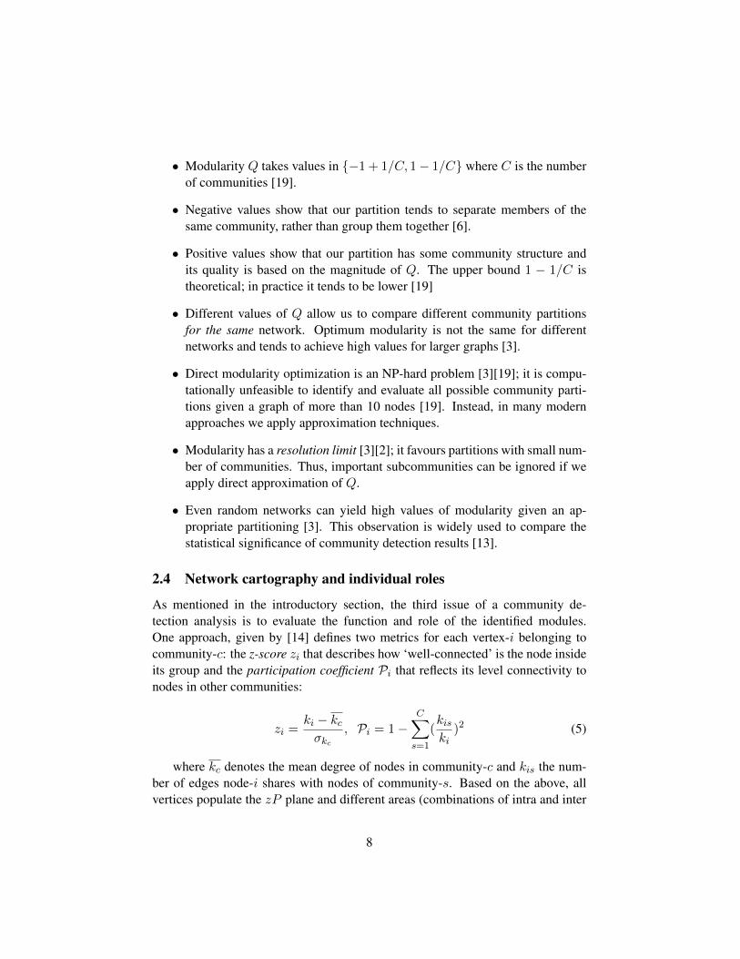
As mentioned in the introductory section, the third issue of a community de-tection analysis is to evaluate the function and role of the identified modules.One approach, given by [14] defines two metrics for each vertex-i belonging tocommunity-c: the z-score zi that describes how ‘well-connected’ is the node insideits group and the participation coefficient Pi that reflects its level connectivity tonodes in other communities:

zi =ki − kcσkc

, Pi = 1−C∑s=1

(kiski

)2 (5)

where kc denotes the mean degree of nodes in community-c and kis the num-ber of edges node-i shares with nodes of community-s. Based on the above, allvertices populate the zP plane and different areas (combinations of intra and inter

8

community participation) reflect different vertex roles; nodes can be classified asperipheral, hubs, brokers between communities, etc. Additionally, based on theconnectivity profile [15] of each role, i.e the tendency of nodes of role 1 to con-nect with ones of role 2, the whole network can be assigned to either the stringy-periphery class (consisting of long chains of peripheral nodes) or the multi-starclass where the majority of nodes tend to connect to a small number of high de-gree ones, creating ‘star-like’ structures. It is important to note that these node andnetwork characterizations, although intuitive, are based on ad-hoc value ranges ofz, P therefore more formal definitions are needed.

3 Community Detection Methods

3.1 Problem description

Community detection methods are algorithms that given a graph G = {V,D}with an adjacency (or weight) matrix A, they output a collection of node groups{gc}Cc=1 that represent a possible partition. The number of communities C andtheir size is not known a-priori (in contrast to the popular Graph Partitioningproblem of combinatorial optimization [2]). For now, we restrict our attentionto non-overlapping communities, thus a node is assigned only to a single group;gi ∩ gj = ∅ ∀i 6= j ∈ {1, ..., C}.

The problem of community detection has many similarities with that of dataclustering from the Unsupervised Learning literature [13]. Labeled examples of themultivariate data are not available (in contrast to the Supervised Learning frame-work), so we have to implement algorithms to find out of how the input observa-tions (mapped on aD-dimensional space whereD is the number of their attributes)is organized into an unknown number of clusters. In the network paradigm, ourdata are in a relational form [13] (vertices connected by edges) so we make infer-ences of their organization based on their topology. At this point it is important tounderline that given a partition of a network into communities, we can not be surethat this solution is unique [2].

Modern community detection methods can be classified into two categories;the first consists of algorithms that partition a graph into communities based ontopological features (such as betweeness centrality [21] etc) and then use modu-larity to evaluate the result. The second consists of algorithms that try to directlyoptimize modularity using some approximation scheme. Another categorization[3] is based on how these algorithms construct the community hierarchy dendo-gram discussed in the previous section; agglomerate methods start by consideringeach individual node to be a community (the leaves at the bottom layer of thedendogram) and proceed constructively by merging partitions based on some simi-

9

larity metric. On the other hand, divisive methods start by the whole graph (parentnode of the dendogram) and break it down into different communities until theyreach a point where each node where we have N communities with a single nodeat each. It is important to note that purely agglomerate or divise methods do notallow overlapping communities.

In the next section we will provide a brief overview of different communitydetection methodologies we studied and implemented. The performance of someof these methods is presented in the Experiments section.

3.2 Agglomerate

Given a collection of nodes V along with their edges D, we define some kindof similarity metric initially between nodes and then between groups, in order tosuccessively merge them together and form the community hierarchy dendogram.Initially we consider that each individual node is a separate group. During the firstiteration we group together each pair i, j of nodes with the highest similarity xij .We proceed by merging pairs of similar groups until we reach the top level of thedendogram where the whole network is a single group. This technique is also calledhierarchical clustering [3] [11]. Unsuprisingly, the performance of these methodsheavily relies on the similarity metric xij itself and some of them are presented inthe paragraphs below.

Distance-based structural equivalence [3] is based on the concept that similarnodes have same neightbours even if they are not adjacent themselves, thus xij =√∑

k 6=i,j(Aik −Ajk)2

Pearson correlation [3] is based on the similar concept of structural equiva-lence, but instead of a distance metric it measures the correlation between rows(or columns) of the adjacency matrix A. So xij =

∑k(Aik−µi)(Ajk−µj)

Nσiσjwhere

µi = 1N

∑j Aij and σi =

∑j(Aij − µi)2.

Donetti-Munoz method [11] that utilizes a matrix L called the Laplacian, de-fined by inverting the sign of each element of A and then setting Aii = ki ∀i ∈{1, ..., N}. The idea is to use the values of D eigenvector components of L andproject each individual to a D-dimensional space. Then, by defining a distance-based similarity measure such as angular or Eucledean distance, we apply hierar-chical clustering to produce a dendogram of possible community partitions. Themain drawback of this method is that the number D of eigenvectors we use is not

10

known a priori and the performance of this method relies on choosing a propervalue of it.

Capocci method [12] utilizes the normal matrix N of A which is defined bydividing each Aij by the sum of the elements of A. Then, similarly using theeigenvectors of N it projects (similarly to Donetti-Munoz) the nodes to a highdimensional space and applies hierarchical clustering for community division. Al-though easy to implement and relatively fast, it yields poor results in most real andartificial networks.

3.3 Divisive

Divisive methods start by considering the whole network as a single communityand proceed deconstructively by breaking it down into smaller ones. Some verypopular and efficient community detection methodologies fall into this categoryand they are presented below.

Newman-Girvan method was first introduced along with the notion of modu-larity in the seminal paper [6]. It utilizes the measure of edge betweeness, usuallydefined by the number of shortest paths between any pair of nodes that run throughthat given edge. Other (and less efficient) formulations are discussed in [6]. Theintuition behind this measure is that communities are linked together by a smallnumber of edges that have significantly higher traffic than the others. The algo-rithm consists of ranking each edge in the network based on that edge centralitymeasure and by removing the most popular one. After the removal all edge be-tweenesses are re-calculated and another edge is removed. The algorithm iteratesas shown above until some part of the network is isolated thus we have communityseparation. We apply the same procedure for each subgraph thus building the com-munity hierarchy dendogram, from which we select the layer with represents thepartition with the highest value of modularity. The algorithm, although very popu-lar, is relatively slow [3] and performs poorly against densely connected graphs.

Spectral partitioning is another divisive method from Mark Newman [8] thatbuilds the community hierarchy dendogram by performing bisections of each com-munity. It utilizes the modularity matrix B defined by Bij = Aij − kikj

2M , whichhas the property that the elements of each of its rows and columns sum to zero. Sogiven the full graph, each bisection is performed by computing the leading eigen-vector of B and by dividing the vertices into two groups according to the signs ofthe elements of this vector. For each subgroup g we perform the same division

11

scheme but with an updated modularity matrix B(g)ij = Bij − δij

∑k∈g Bik. The

method is relatively fast and has the excellent property of identifying undivisiblegroups; a community can not have further divisions with positive modularity if theall the eigenvalues of the modularity matrix are non-positive. It also provides goodresults in most real and artificial problems (see Experiments section).

Extremal optimization [9] is a method for direct approximation of the modu-larity function Q. Given a network and a community partition, it breaks down itsmodularity Q into the individual contributions from each node. So given a node-ibelonging to community-r, its contribution to the overall modularity is calculatedfrom:

λi =kr(i)

ki− ar(i) (6)

where kr(i) is the number of neighbours of i that belong to the same commu-nity as i (intra-community degree) and ar(i) is the r-element of the a vector usedin (4). The quantity λi is normalized to the interval [-1,1] to allow comparisonsbetween individual nodes and the overall modularity can be easily recovered byQ = 1

2M

∑Ni=1 kiλi.

The algorithm starts by creating a random bisection of the original graph. Thenit calculates the lamdas for each node and moves the least contributing nodes to an-other group. Due to the random initialization scheme and to avoid local maxima weusually select randomly one of the n-least contributing nodes to change its mem-bership. After a number of moves, if the modularity does not improve we proceedrecursively by applying the algorithm to each partition. From the resulting den-dogram we select the partition with the highest modularity. Although the methodis heavily initialization dependent [9] it provides state-of-the-art results in mostproblems (see Experiments section).

3.4 Other

In this section we examine methodologies which do not build a community hier-archy dendogram but examine different partitions (solutions) to maximize a utilityfunction.

Simulated annealing [14] [3] is a popular method for global optimization in-spired by the annealing technique in metallurgy. In the community detection frame-work, we seek to optimize Q. Thus, during each step we perform explorations intodifferent partitions of the network and for a k-step of the algorithm we accept asolution with probability p:

12

p =

{1 if Q is increased

e−∆QT otherwise

where ∆Q = Q(k) − Q(k+1) and T a computational temperature. The intro-duction of T , which decreases during each step of the algorithm by T (k+1) = cT (k)

(where usually c = 0.995), makes the selection of low Q solutions more probablefor the initial iterations, but less likely to be accepted during the consequent steps.The reason we allow the selection of partitions with Q(k) > Q(k+1) is to avoidgetting trapped into local maxima; we start the algorithm with a random initializa-tion of partitions and a low value of T gives a higher freedom to explore possiblesolutions. As the algorithm converges to an area of ‘good’ solutions, the modelbecomes very strict and does not allow selections that decrease Q.

The solution exploration scheme consists of N2 local and N global ‘moves’,where N is the total number of nodes. The local moves consist of assigning anindividual node to a different partition, while global moves consist of mergingor splitting whole partitions. Thus, although the algorithm is very popular forgeneral optimization problems, for the community detection framework it is verycomputationally demanding [3].

The Potts method [13] is a community detection algorithm inspired by Statis-tical Mechanics. The model assumes that a network is a system of spins that canhave q different states. Thus, each node-i can take have a spin value σi ∈ {1, ..., q}(that basically accounts for its community membership, C = q) and the interactionenergy between spins is given by −Jij (where J = A) if the spins are in the samestate and zero if they are not. Finding the appropriate partition for the networkequals to finding the ground state (minimum) of the Hamiltonian:

H = −Jij∑i,j∈N

δσi,σj + γ

q∑s=1

ns(ns − 1)

2(7)

where ns is the number of spins (nodes) in state (community) s, Jij the interac-tion strength (given by the adjacency or weight matrix A), γ a positive parameterand the Kronecker δσi,σj is 1 if i, j have the same spin (belong to the same com-munity) or 0 otherwise. The above equation reflects the two competing forces inour system; the first term of the summand favours a homogeneous distribution ofspins (minimum for all i, j in the same community) while the second term favoursa uniform distribution of spins across nodes. To find the ground state (minimum)of the above system we employ a Monte Carlo single spin flip heat-bath algorithm

13

along with simulated annealing. The method is fast and provides very competitiveresults for most real-world and artificial datasets.

The computational complexity of a variety of different community detectionalgorithms is presented in [16].

4 Experiments

Our preliminary study involved a comparative analysis of different community de-tection algorithms across real world (see Table 1) and computer generated networkdatasets (see Table 2). From the outcome of this small scale research we expectto derive some general conclusions on the performance of different clustering al-gorithms using a variety of metrics. Additionally we present the performance ofNMF, a novel probabilistic community detection algorithm based on non-negativematrix factorization that produces state-of-the-art results in most problems andgives a promising research direction.

Table 1: Real-world networksName N M weighted?

Zachary’s karate [22] 34 77 noSouthern women [23] 18 139 yes

Jazz musicians [24] 198 2742 noDolphins [25] 62 159 no

Great Tits subset 49 738 yes

4.1 Set-up

As mentioned previously, our experimentation involved a comparative analysis ofdifferent methods across real and artificial datasets. For the real datasets we usedsome very popular networks which are widely adopted as performance benchmarksin the vast majority of the community detection literature. The detailed list ispresented on Table 1.

For those real-world networks and like any other data clustering problem, weusually do not have an observed solution i.e a collection of communities that rep-resent the real partition of the graph. For that reason, we have also generated acollection of artificial networks with observed community structure, in order toevaluate the performance of our algorithms not only in terms of the modularity butalso in terms of how similar the produced groups of our algorithms are to the realones.

14

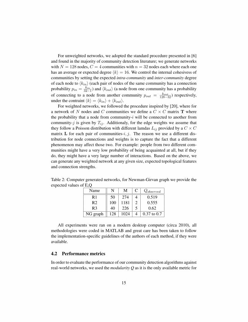
For unweighted networks, we adopted the standard procedure presented in [6]and found in the majority of community detection literature; we generate networkswithN = 128 nodes, C = 4 communities with n = 32 nodes each where each onehas an average or expected degree 〈k〉 = 16. We control the internal cohesivess ofcommunities by setting the expected intra-community and inter-community degreeof each node to 〈kin〉 (each pair of nodes of the same community has a connectionprobability pin = kin

32−1 ) and 〈kout〉 (a node from one community has a probabilityof connecting to a node from another community pout = kout

128−32 ) respectively,under the contraint 〈k〉 = 〈kin〉+ 〈kout〉.

For weighted networks, we followed the procedure inspired by [20], where fora network of N nodes and C communities we define a C × C matrix T wherethe probability that a node from community-i will be connected to another fromcommunity-j is given by Tij . Additionaly, for the edge weights we assume thatthey follow a Poisson distribution with different lamdas Lij provided by a C × Cmatrix L for each pair of communities-i, j. The reason we use a different dis-tribution for node connections and weights is to capture the fact that a differentphenomenon may affect those two. For example: people from two different com-munities might have a very low probability of being acquainted at all, but if theydo, they might have a very large number of interactions. Based on the above, wecan generate any weighted network at any given size, expected topological featuresand connection strengths.

Table 2: Computer generated networks, for Newman-Girvan graph we provide theexpected values of E,Q

Name N M C Qobserved

R1 50 274 4 0.519R2 100 1181 2 0.555R3 40 226 5 0.62

NG graph 128 1024 4 0.37 to 0.7

All experiments were ran on a modern desktop computer (circa 2010), allmethodologies were coded in MATLAB and great care has been taken to followthe implementation-specific guidelines of the authors of each method, if they wereavailable.

4.2 Performance metrics

In order to evaluate the performance of our community detection algorithms againstreal-world networks, we used the modularity Q as it is the only available metric for

15

unobserved datasets. We expect that an efficient algorithm will achieve competitiveresults against other methods in the literature.

For observed datasets, apart from Q we make use of the information that thecommunity partitions are already known. Thus, we need to measure the similaritybetween the observed partitions {g(o)c}

Coc=1 and the ones produced by our algo-

rithm {g(f)c}Cf

c=1. We notice that we might get a different number of communitiesfrom the ones observed; some might be split or merged into others. For that reason,we follow an approach from information theory presented in [16] by estimating thenormalized mutual information. We define aC×C confusion matrix N where rowscorrespond to the observed commmunities and columns correspond to the ‘found’communnities. Each element Nij is the number of nodes in the real community-ithat appear in the found community-j. Thus the similarity between the two parti-tions {g(o)c}

Coc=1 and {g(f)c}

Cf

c=1 is:

I(g(o),g(f)) =−2∑Co

i=1

∑Cf

j=1Nij logNijNNi∗∑Co

i=1Ni∗ log Ni∗N +

∑Cf

j=1N∗j logN∗jN

(8)

where Co and Cf are the number of communities found in the observed andfound partition respectively, Ni∗ the sum of elements of the i-th row of N, N∗jthe sum of elements of the j-th column of N and N the sum of elements of theconfusion matrix N. The quantity I takes values from 0 to 1 and measures theamount of information correctly extracted by the algorithm [16]. Other measures,such as the Rand similarity metric are presented in [17].

Finally, another important performance metric is the statistical significance ofthe extracted community structure. Given a partitioning {g(f)c}

Cf

c=1, each commu-nity g(f)c has say n nodes, lin intra-community and lout inter-community links. Byfollowing [13], we calculate the expected number of possible equivalent commu-nities E(n, lin, lout) in a random network of the same size (N nodes, M edges)where the connection probability is P (Aij = 1) = 2M

N(N−1) for i 6= j:

E(n, lin, lout) =

(N

n

)(n(n−1)2

lin

)(n(N − n)

lout

)plin (9)

×(1− p)n(n−1)/2−loutplout(1− p)n(N−n)−lout (10)

where if E(n, lin, lout) > 1 then it is likely to find one such a community in arandom graph of the same size, marking the border of statistical significance [13].

We conclude this section by raising an important issue: it is accepted in thecommunity detection literature that algorithms that seek to directly optimize mod-ularity perform better than the ones that simply use it as a performance metric.

16

From our point of view, we consider that defining a performance metric and basedon that, comparing an algorithm that uses it for evaluation purposes and anotherthat tries to directly optimize it, creates biased results towards the latter.

4.3 Sensitivity analysis

As mentioned in the previous section, our comparative analysis involved the per-formance evaluation of different community detection algorithms, across a varietyof datasets. Although good results at a variety of benchmark datasets provide agood indication for the competitiveness of a method, we need further confirma-tion that the results are not dataset-specific. Additionally, we are interested in theperformance of the algorithm in cases we have missing observations or fuzzy com-munity structure. For that reason, we have designed a variety of tests for weightedand unweighted networks to evaluate their resilience in cases where the communitystructure of the same network is not apparent; communities are loosely connectedor observations are knocked-out.

For unweighted networks, we used the Newman-Girvan random graph [6] de-scribed in the ‘Set-up’ section. As mentioned previously, we can control intra-community density by manipulating the values of 〈kout〉 and 〈kin〉, which basicallyare the probabilities that nodes from different and the same community are con-nected. Therefore, starting with a densely connected graph (〈kout〉 = 1,〈kin〉 =15) and by increasing 〈kout〉 (thus decreasing 〈kin〉) we make the communitiesmore loosely connected. We run our algorithms for each value of 〈kout〉 to iden-tify how the performance of each one drops as the network becomes fuzzier. Oursensitivity analysis scheme is shown in Algorithm 1.

[ht] Sensitivity analysis for Newman-Girvan random graphs [1] Set 〈kout〉 ←1, thus 〈kin〉 = 15 because 〈k〉 = 〈kin〉 + 〈kout〉. 〈kout〉 ≤ 8 generate 100Newman-Girvan random graphs (N = 128, C = 4, n = 32) with the given〈kout〉, 〈kin〉. run community detection for those graphs using each of the avail-able methods. Get Q(kout)

mean and I(kout)mean . Set 〈kout〉 ← 〈kout〉 + 1, thus making thenetwork ‘fuzzier’ Plot Qmean, Imean across different values of 〈kout〉

For weighted networks generated by the procedure we described at the ‘Set-up’section we follow a different approach. For simplicity we assume that the weightsAij take integer values and under a social network context, 1 unit of weight reflectsone unit of ‘co-existence’ or ‘co-occurence’ of two individuals given a time-frame;for example Aij can be the number of emails exchanged between two people perday, or the number of occurences of two animals in the same location per hour. Weassume that each unit of co-occurence is captured by a sensor that can be faulty,i.e it can successfully capture an observation with probability psensor. Therefore,we generate samples of the weights matrix A of the network for different values

17

of psensor and run our community detection methods in order to evaluate theirperformance. Our methodology is shown in Algorithm 2 and emulates the real-world problem of capturing bird positions at Wytham Woods, Oxford.

[ht] Sampling weighted networks using the faulty sensor scheme [1] psensor ={0.9, 0.7, 0.4}Generate 25 weight matrices W whereWij follows a binomial dis-tribution with n = Aij and p = psensor run community detection for those graphsusing each of the available methods. Get Q(kout)

mean and I(kout)mean . Plot Qmean, Imeanacross different values of psensor

4.4 Results

In this section we present the results of our experiments for each community detec-tion method and dataset. Our focus is to compare the performance of the alreadyexisting methods against the novel probabilistic NMF algorithm and evaluate itspotential for further research.

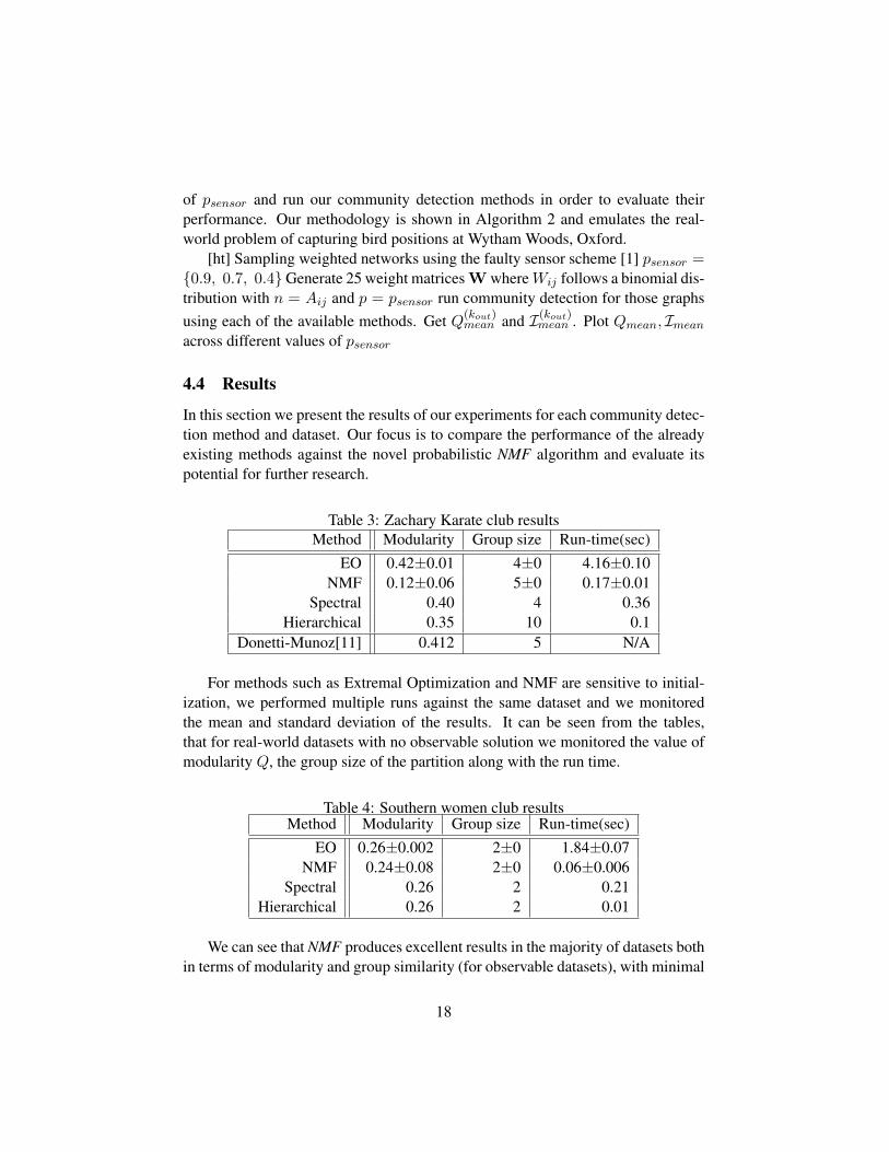
Table 3: Zachary Karate club resultsMethod Modularity Group size Run-time(sec)

EO 0.42±0.01 4±0 4.16±0.10NMF 0.12±0.06 5±0 0.17±0.01

Spectral 0.40 4 0.36Hierarchical 0.35 10 0.1

Donetti-Munoz[11] 0.412 5 N/A

For methods such as Extremal Optimization and NMF are sensitive to initial-ization, we performed multiple runs against the same dataset and we monitoredthe mean and standard deviation of the results. It can be seen from the tables,that for real-world datasets with no observable solution we monitored the value ofmodularity Q, the group size of the partition along with the run time.

Table 4: Southern women club resultsMethod Modularity Group size Run-time(sec)

EO 0.26±0.002 2±0 1.84±0.07NMF 0.24±0.08 2±0 0.06±0.006

Spectral 0.26 2 0.21Hierarchical 0.26 2 0.01

We can see that NMF produces excellent results in the majority of datasets bothin terms of modularity and group similarity (for observable datasets), with minimal

18

computational effort.

Table 5: Jazz musicians resultsMethod Modularity Group size Run-time(sec)

EO 0.42±0.007 4±0 74.157±1.84NMF 0.42±0.008 7±0 2.09±0.15

Spectral 0.39 3 1.01Hierarchical 0.34 13 0.56

Table 6: Dophin social network resultsMethod Modularity Group size Run-time(sec)

EO 0.51±0.006 4±0 11.24±0.428NMF 0.466±0.033 7±0 0.334±0.030

Spectral 0.491 5 0.44Hierarchical 0.455 12 0.13

Table 7: Wytham Woods Great Tit subset resultsMethod Modularity Group size Run-time(sec)

EO 0.35± ε 2±0 6.73±0.18NMF 0.35± ε 3±0 0.25±0.036

Spectral 0.35 2 0.3Hierarchical 0.3 5 0.09

Additionally, for the artificial datasets in Tables 9 and 10, NMF correctly ex-tracts the exact original community structure, with speed that is many levels ofmagnitude below the second best performing method, Extremal Optimization.

For unweighted networks, we performed sensitivity analysis for the Newman-Girvan random graph, using an approach described in the previous section. The re-sults, presented in Fig. 4 and 5 show the performance of each method across differ-ent levels of community cohesion. We can see that for increasing inter-communitydegree 〈kout〉, modularity and group identification fall as the community struc-ture of the graph becomes fuzzier. Although Spectral Partitioning and Hierarchicalclustering perform poorly, Extremal Optimization and NMF have a more stablebehaviour extracting modular structure that is similar to the observed one.

We also performed sensitivity analysis on weighted networks, following thesensor emulation scheme described in the previous section. For the three fully

19

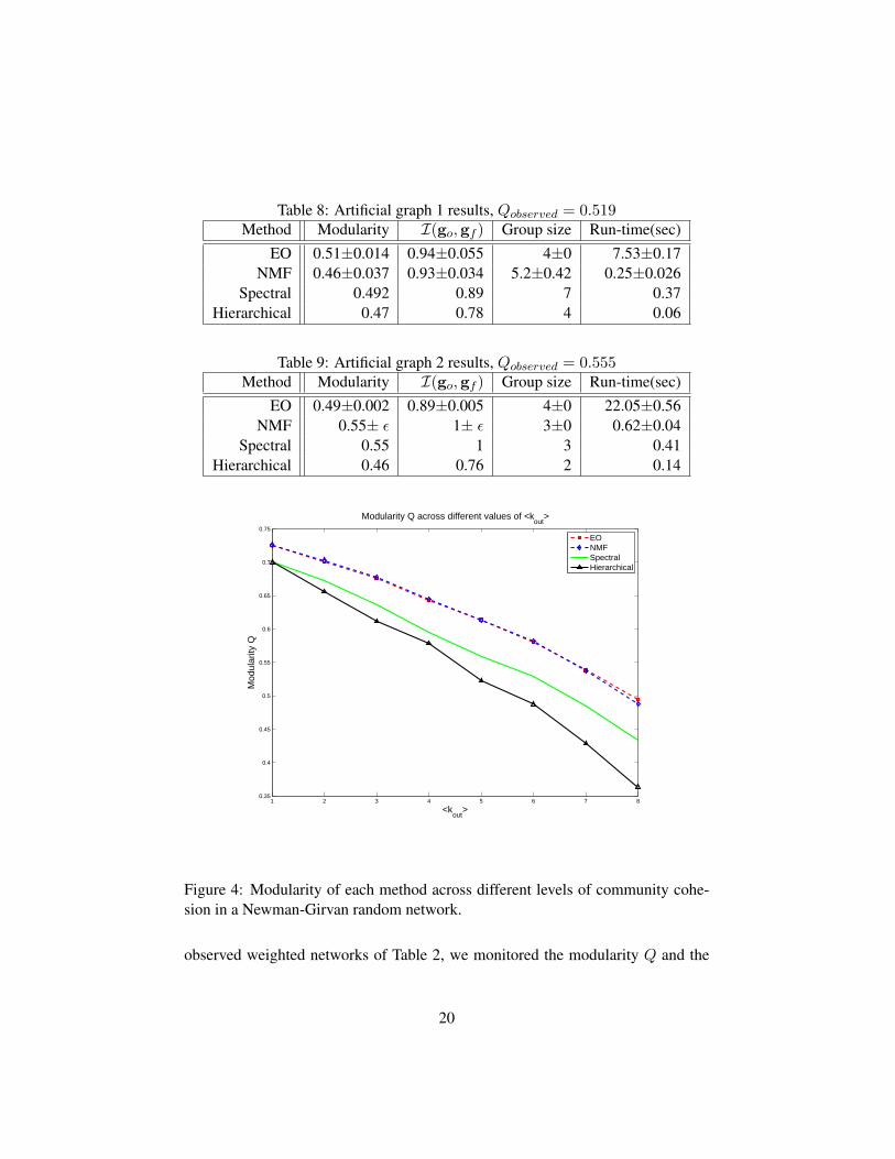
Table 8: Artificial graph 1 results, Qobserved = 0.519Method Modularity I(go,gf ) Group size Run-time(sec)

EO 0.51±0.014 0.94±0.055 4±0 7.53±0.17NMF 0.46±0.037 0.93±0.034 5.2±0.42 0.25±0.026

Spectral 0.492 0.89 7 0.37Hierarchical 0.47 0.78 4 0.06

Table 9: Artificial graph 2 results, Qobserved = 0.555Method Modularity I(go,gf ) Group size Run-time(sec)

EO 0.49±0.002 0.89±0.005 4±0 22.05±0.56NMF 0.55± ε 1± ε 3±0 0.62±0.04

Spectral 0.55 1 3 0.41Hierarchical 0.46 0.76 2 0.14

1 2 3 4 5 6 7 80.35

0.4

0.45

0.5

0.55

0.6

0.65

0.7

0.75

<kout

>

Mod

ular

ity Q

Modularity Q across different values of <kout

>

EONMFSpectralHierarchical

Figure 4: Modularity of each method across different levels of community cohe-sion in a Newman-Girvan random network.

observed weighted networks of Table 2, we monitored the modularity Q and the

20

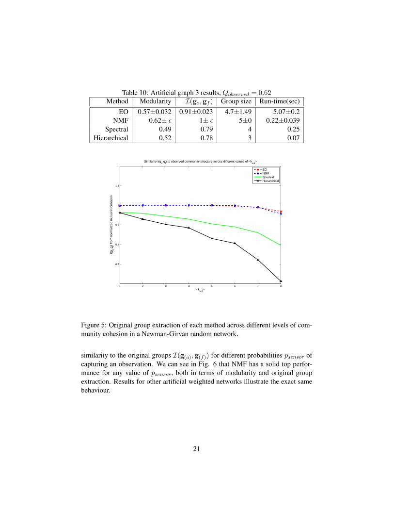
Table 10: Artificial graph 3 results, Qobserved = 0.62Method Modularity I(go,gf ) Group size Run-time(sec)

EO 0.57±0.032 0.91±0.023 4.7±1.49 5.07±0.2NMF 0.62± ε 1± ε 5±0 0.22±0.039

Spectral 0.49 0.79 4 0.25Hierarchical 0.52 0.78 3 0.07

1 2 3 4 5 6 7 8

0.7

0.8

0.9

1

1.1

Similarity I(go,g

f) to observed community structure across different values of <k

out>

I(g o,g

f) fr

om n

orm

aliz

ed m

utua

l inf

orm

atio

n

<kout

>

EONMFSpectralHierarchical

Figure 5: Original group extraction of each method across different levels of com-munity cohesion in a Newman-Girvan random network.

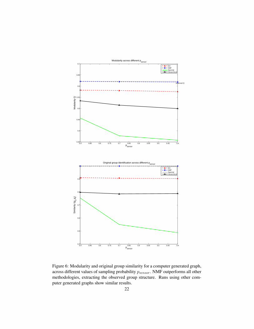
similarity to the original groups I(g(o),g(f)) for different probabilities psensor ofcapturing an observation. We can see in Fig. 6 that NMF has a solid top perfor-mance for any value of psensor, both in terms of modularity and original groupextraction. Results for other artificial weighted networks illustrate the exact samebehaviour.

21

0.40.450.50.550.60.650.70.750.80.850.90.35

0.4

0.45

0.5

0.55

0.6

0.65

0.7

Modularity across different psensor

psensor

Mod

ular

ity Q

observed Q

EONMFSpectralHierarchical

0.40.450.50.550.60.650.70.750.80.850.90.4

0.5

0.6

0.7

0.8

0.9

1

Original group identification across different psensor

psensor

Sim

ilarit

y I(

g o,gf)

EONMFSpectralHierarchical

Figure 6: Modularity and original group similarity for a computer generated graph,across different values of sampling probability psensor. NMF outperforms all othermethodologies, extracting the observed group structure. Runs using other com-puter generated graphs show similar results.

22

5 Conclusion and closing thoughts

In this work we provided a short ‘research diary’ of the community detection no-tions and methods we studied since the beginning of the project. While it is ac-knowledged that ‘most accurate methods tend to be more computationally expen-sive’ [16], we demonstrated how the novel NMF algorithm can provide state of theart results in community detection problems with minimal computational effort,showing a promising direction for our research from this point on.

NMF does not only provide competitive results against other popular commu-nity detection methods in terms of modularity and original group identificationwith minimal computational effort; it also provides probabilistic outputs for com-munity membership of each node. The existing methodologies described in pre-vious sections assign each node to a single group based on some educated harddecision. Now matter how correct such an assignment is, it completely omits com-munity overlap, which is an imporant aspect of real world networks. Most standardmethodologies handle multi-group membership by performing multiple runs withdifferent initialization parameters and based on a concordance matrix, they evalu-ate the stability of node assignments, i.e how frequently each node appears in thesame community.

NMF explicitly handles multi-community membership on a single run by pro-viding for each individual node-i a group membership distribution; given a parti-tion {gc}Cc=1, for each group-c we have a probability P (i ∈ gc) that the node-iwill belong to the group c. Another way of expressing it is that each element of thecommunity matrix P of Eq. (4) now expresses a probability for group member-ship rather than a hard binary decision. This is illustrated in Fig. 7 on a computergenerated dataset with overlapping community structure.

Thus instead of following a frequentist approach, using the group membershipdistribution we capture our degree of belief for the assignment of each node. Theadvantages of such probabilistic outputs are:

• we describe multi-community membership of each node in a formal way.

• we identify overlapping communities based on the probability mass of theirnodes.

• model our prediction error in problems with assymmetric misclassificationcosts.

• we can implement community-wise descriptive graph visualization tools.

• we can now formally measure the ‘fuzziness’ of a network, based on theentropy of the group membership distribution of each node. For example,

23

12

34

5

0

2

4

6

8

10

12

14

16

18

20

0

0.2

0.4

0.6

0.8

1

Communities

Membership distributions for 19 nodes and 5 extracted communities

Individual nodes

Mem

bers

hip

prob

abili

ty

Figure 7: Membership probabilities (z-axis) for a network of 19 nodes (y-axis) and5 identified communities (x-axis) in a computer generated graph. Given a node, thebars across the x-axis represent the community membership distribution. We cansee that there are nodes with different degree of participation across communities.

given 4 communities, if the membership distribution is near ‘random guess’i.e 25% probability that node-i will belong to each group, then this loss ofconfidence yields a high entropy value.

• the network cartography and individual ‘role assignment’ techniques (basedon intra and inter community participation coefficients of [14]) we describedin previous section can be improved under a probabilistic framework.

• we can make informed predictions on issues such as group stability overtime; for example between fuzzy communities we can expect a larger ex-change of nodes and phenomena such as fission-fussion can be described ina formal way.

• based on how probability membership distributions change over time, we

24

can make informed predictions on events such as an individual from groupA and another from group B will belong to the same group after a period oftime.

Based on the above, we conclude by stating that our research has the potentialof a) improving already existing and well-acknowledged methods, b) introducingnovel methodologies in the study of networks with the potential of wide adoptionand c) providing important context-specific insights on applications such as ourGreat Tit social network study at Wytham Woods.

25

References

[1] M.E.J Newman - The structure and function of complex networks, SIAM Re-view 45, 167-256 (2003)

[2] Mason A. Porter, Jukka Pekka Onnela and Peter J. Mucha - Communities inNetworks, Notices of the American Mathematical Society, Vol. 56, No. 9, 2009

[3] Santo Fortunato and Claudio Castellano - Community Structure in Graphs,chapter of Springer’s Encyclopedia of Complexity and System Science (2008)

[4] Andrew Sih, Sean F. Hanser, Katherine A McHugh - Social Network The-ory: new insights and issues for behavioral ecologisits, Behav Ecol Sociobiol(2009) 63:975-988

[5] Alain Barrat, Marc Barthelemy and Alessandro Vespignani Modeling the evo-lution of weighted networks, Physical Review E 70, 066149 (2004)

[6] M.E.J Newman and M. Girvan - Finding and evaluating community structurein networks, Phys. Rev. E 69, 026113 (2004)

[7] M.E.J Newman - Analysis of weighted networks, Phys. Rev. E70,056131(2004)

[8] M.E.J Newman - Modularity and community structure in networks, PNAS June6, 2006 vol. 103 no. 23 8577-8582

[9] Jordi Durch and Alex Arenas - Community detection in complex networks us-ing extremal optimization. PHYSICAL REVIEW E72, 027104 (2005)

[10] Ying Fan, Menghui Li, Pen Zhang, Jinshan Wu, Zengru Di - Accuracy andprecision of methods for community identification in weighted networks, Phys-ica A 377 (2007) 363-372

[11] Loca Donetti and Miguel A Munoz - Detecting network communities: a newsystematic and efficient algorithm, Journal of Statistical Mechanics: Theoryand Experiment (2004)

[12] Cappocci A, Servedio VDP, Caldarelli G, Colaiori F - Detecting communitiesin large networks, Physica A. Vol 352, No 2-4, pp 669-676

[13] Jorg Reichardt and Stefan Bornholdt - Detecting Fuzzy Community Structuresin Complex Networks with a Potts Model, Physical Review Letters Volume 93,Number 21 (2004)

26

[14] Guimer R, Amaral LA - Cartography of complex networks: modules anduniversal roles, J Stat Mech. (2005)

[15] Roger Guimer , Marta Sales-Pardo and Lus A. N. Amaral - Classes of com-plex networks defined by role-to-role connectivity profiles, Nature Physics 3,63 - 69 (2007)

[16] Leon Danon, Albert Daz-Guilera, Jordi Duch and Alex Arenas - Comparingcommunity structure identification, Journal of Statistical Mechanics: Theoryand Experiment, Volume 2005, September 2005

[17] Amanda L. Traud, Eric D. Kelsic, Peter J. Mucha, Mason A. Porter - Com-munity Structure in Online Collegiate Social Networks, Physics and Society(2008)

[18] Aaron Clauset Cristopher Moore and M. E. J. Newman - Hierarchical struc-ture and the prediction of missing links in networks, Nature 453, 98-101 (1May 2008)

[19] Erik Holmstrom, Nicolas Bock, Johan Brannlund - Modularity density of net-work community divisions, Physica D 238 (2009) 1161-1167

[20] Mark Ebden - Towards plan detection using message passing, Pattern Analy-sis and Machine Learning Group report, 18 November 2009

[21] L.C. Freeman - A set of measures of centrality based upon betweeness, So-ciometry, 40 (1977), pp. 35-41

[22] W. W. Zachary - An information flow model for conflict and fission in smallgroups, Journal of Anthropological Research 33, 452-473 (1977)

[23] Breiger R. - The duality of persons and groups Social Forces, 53, 181-190(1974)

[24] P.Gleiser and L. Danon , Adv. Complex Syst.6, 565 (2003)

[25] D. Lusseau, K. Schneider, O. J. Boisseau, P. Haase, E. Slooten, and S. M.Dawson - Behavioral Ecology and Sociobiology 54, 396-405 (2003)

27