EM 437

COMMUNICATION SYSTEMS II

LABORATORY MANUAL

2006-2007 FALL

2

TABLE OF CONTENTS

page

LABORATORY RULES ...................................................................................................................3

CHAPTER 1: PULSE CODE MODULATION ..............................................................................4

1. 1. Introduction ................................................................................................................................4

1. 2. The Apparatus ............................................................................................................................4

1. 3. The Modulation Process ............................................................................................................4

1. 4. Quantising Noise.........................................................................................................................6

1. 5. References ...................................................................................................................................8

CHAPTER 2: SAMPLING AND TIME DIVISION MULTIPLEX .............................................9

2. 1. Introduction ................................................................................................................................9

2. 2. The Apparatus ............................................................................................................................9

2. 3. The Sampling Process-Theory ..................................................................................................9

2. 4. Time Division Multiplexing .....................................................................................................14

2. 5. Observation of Signals .............................................................................................................14

2. 6. References .................................................................................................................................15

Appendix 1. Convolution .................................................................................................................16

EXPERIMENT 1 : PCM – CODING .............................................................................................17

EXPERIMENT 2 : PCM – QUANTISING LEVELS...................................................................20

EXPERIMENT 3 : PCM – QUANTISING NOISE ......................................................................22

EXPERIMENT 4: SAMPLING AND TIME DIVISION MULTIPLEX....................................26

3

Gazi University Department of Electrical and Electronics Engineering

EM437 Communication Systems II Lab.

LABORATORY RULES

• Everyone should attend experiments on the determined days and hours. • If one does not attend more than one experiment he/she will take the grade DY. • There will be four experiments. • Reports should include:

Name and number of writer Name, purpose, theory and the procedure of experiment Comments of writer

• There will be a quiz for every experiment. • Grading will be as follows:

Experiments : 25% Quiz : 25% Performance : 10% Final Examination : 40%

4

CHAPTER 1: PULSE CODE MODULATION

1. 1. Introduction

Pulse Code Modulation(PCM) is by far the most important digital modulation method. It is used extensively in data and communication channels and is widely used for transmission of telephony between exchanges. In fact the words ‘analogue-to-digital conversion’ (A/D) often imply PCM although other A/D methods such as delta modulation are possible. In PCM the analogue signal is first sampled and the amplitude of each sample is used to encode a stream of pulses. The coding used is often binary because binary electronic devices are cheap. 1. 2. The Apparatus

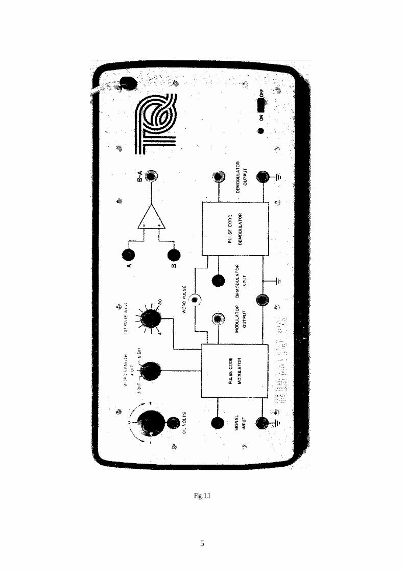
Fig.1.1 shows the apparatus, which comprises a pulse code modulator and demodulator. The input to the modulator can have a signal of any waveform or amplitude applied to it, and a separate d.c. level control is supplied on the equipment. A choice of 3,4 or 8 bit encoding is available at the modulator. The signal can be reconstituted by the pulse code demodulator. A difference amplifier is also supplied to allow the signal into the p.c.m modulator to be compared with the signal out of the p.c.m demodulator in order to establish the loss of information(i.e. added noise) as a function of the encoding, frequency and amplitude of the input signal. The following additional apparatus is required:

(a) Audio Signal Generator (b) Oscilloscope

1. 3. The Modulation Process

The signal to be transmitted is first sampled. As demonstrated in the experiment E15g(Sampling and Time Division Multiplex), the sampling rate should be at least twice the highest frequency in the waveform, otherwise aliasing distortion will occur. Each sample is then encoded into an m-bit binary word. The choice of the number of bits per word(m) is rather important and as usual there is a conflict between opposing considerations. On the one hand m bits means that there can only be 2m possible codes to described the sample amplitude. On the other hand large values of a m mean that a higher bit rate is needed to transmit the required number of samples per second. Thus the system design requires that the minimum value of m be chosen which is consistent with adequate the signal with an m bit code.

If m is chosen to be 3 then there 8 possible amplitude levels, thus,

Code Level 111 7 110 6 101 5 100 4 011 3 010 2 001 1 000 0

5

Fig. 1.1

6

A 3-bit code means therefore that signal only be described by 8 voltages.

This may be demonstrated on the apparatus using the d.c. supply provided. This should be connected to the signal input and the code at the modulator output can be observed on the oscilloscope. It is necessary to identify the beginning of a code word and this is achieved by simultaneously displaying the word pulse. The decoded d.c voltage levels can be observed at the demodulator output after connecting the demodulator to the modulator. In this way the voltage levels for each of the 8 possibilities can be established.

The experiment should be repeated for a 4-bit code with its 16 possibilities, and an 8 bit code with its 256 possibilities.

1. 4. Quantising Noise

When a 3-bit word is being used there are only 8 possible amplitudes that can be transmitted and there is therefore an error between the actual level of the signal and the transmitted signal. The process of making the amplitudes of the samples correspond to discrete levels is termed quantising and the amplitude errors introduced constitute quantising noise. Fig.1.2 shows an analogue signal and its quantised version. The error signal, also shown, is the quantised signal subtracted from the analogue signal.

If the voltage difference between the quantising levels is s then the error signal is a sawtooth-like waveform of peak-to-peak amplitude s. the mean square value of such a waveform is s2/12 and so this quantifies the noise in PCM systems. The fact that this noise waveform contains very high frequencies does not affect the amount of noise falling into the signal board because of the sampling process.

Now we have to decide what the value of s is. Suppose that level 0 in a 3-bit system is –Vc volts and level 7 is +Vc volts then the value of s is 2 Vc/7, or in general

s= 2 Vc / (2m-1) ……………. (1.1)

Fig. 1.2

S

Signal

S

Error signal

Quantised signal

7

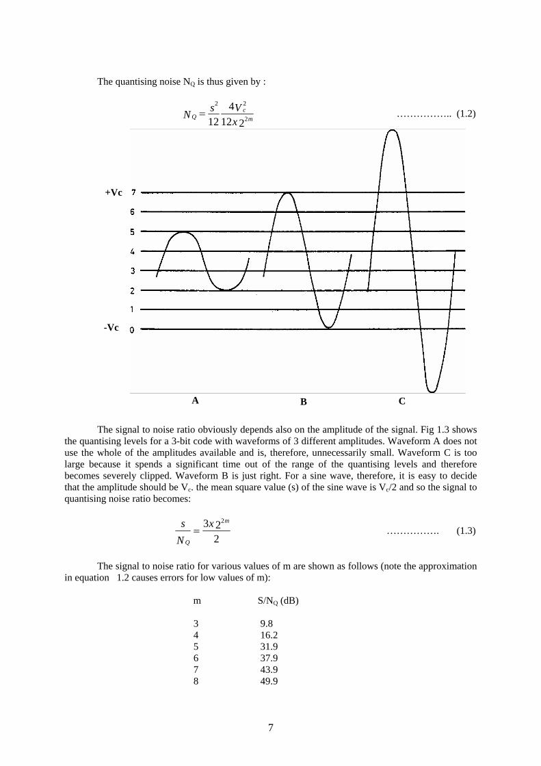
The quantising noise NQ is thus given by :

212

412 2

22

mc

Q xVsN = …………….. (1.2)

The signal to noise ratio obviously depends also on the amplitude of the signal. Fig 1.3 shows

the quantising levels for a 3-bit code with waveforms of 3 different amplitudes. Waveform A does not use the whole of the amplitudes available and is, therefore, unnecessarily small. Waveform C is too large because it spends a significant time out of the range of the quantising levels and therefore becomes severely clipped. Waveform B is just right. For a sine wave, therefore, it is easy to decide that the amplitude should be Vc. the mean square value (s) of the sine wave is Vc/2 and so the signal to quantising noise ratio becomes:

223 2m

Q

xNs

= ……………. (1.3)

The signal to noise ratio for various values of m are shown as follows (note the approximation

in equation 1.2 causes errors for low values of m): m S/NQ (dB)

3 9.8 4 16.2 5 31.9 6 37.9 7 43.9 8 49.9

A

+Vc

-Vc

B C

8

For signals with noise-like characteristics the problem is more difficult because it is not so easy to decide what the optimum amplitude should be. For speech signals there is the additional problem that some people talk loudly and others talk more quietly. Often the quantising grids are unevenly spaced giving a process called companding and this more nearly matches the quantising grid to the statistics of the signal.

The quantising of a sinusoidal signal can be observed by applying a signal of 100 Hz to the signal input and adjusting the oscilloscope for stable triggering. The modulator output can be seen to be cyclically reading through the code alphabet. By connecting the modulator output to the demodulator input and observing the demodulator output, the quantising effect of the pulse code modulation process can be clearly seen.

The amplitude of the signal should now be increased so that it exceeds the extreme levels as determined by the d.c. test. Clipping of the sinusoidal signal can now be observed, high amplitudes leading to longer times during which the sinusoid is clipped.

Applying a sinusoidal signal to both the signal input to terminal B of the difference amplifier, and connecting the demodulator output to terminal A, allows the quantising noise to be examined. The observed shapes should be explained as the amplitude, bits per word, bit rate and input signal frequency are varied. If an r.m.s. meter is available it can be used to measure the quantising noise power and the signal input power. This measurement can be made for various input amplitudes and a graph plotted of signal to noise ratio versus input amplitude. As explained above this should peak when the signal amplitude is near Vc and the signal to noise ratio is then given by equation 1.3.

1. 5. References

1. P.B. Johns T.R. Rowbotham, “Communications Systems Analysis”, Butterworth 1972. 2. J.A. Betts, “Signal Processing, Modulation and Noise”, English Universities 1970.

9

CHAPTER 2: SAMPLING AND TIME DIVISION MULTIPLEX

2. 1. Introduction

In all telecommunications networks there is a need to interconnect switching centers and

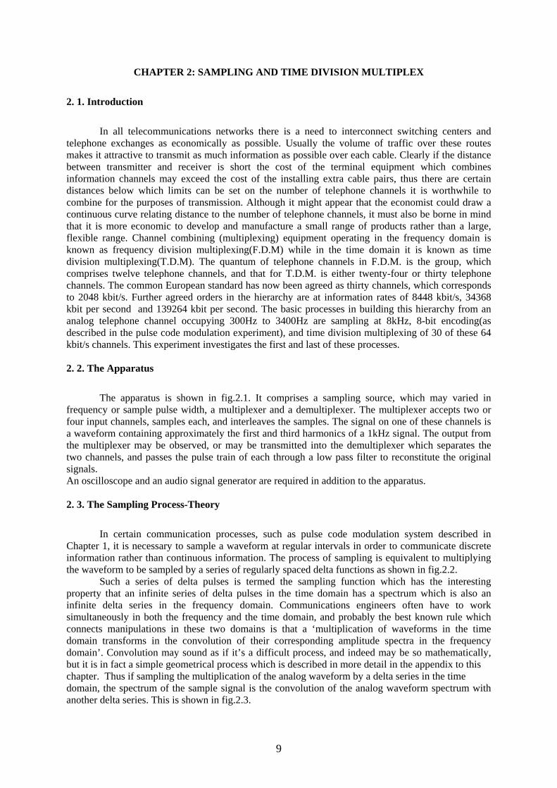
telephone exchanges as economically as possible. Usually the volume of traffic over these routes makes it attractive to transmit as much information as possible over each cable. Clearly if the distance between transmitter and receiver is short the cost of the terminal equipment which combines information channels may exceed the cost of the installing extra cable pairs, thus there are certain distances below which limits can be set on the number of telephone channels it is worthwhile to combine for the purposes of transmission. Although it might appear that the economist could draw a continuous curve relating distance to the number of telephone channels, it must also be borne in mind that it is more economic to develop and manufacture a small range of products rather than a large, flexible range. Channel combining (multiplexing) equipment operating in the frequency domain is known as frequency division multiplexing(F.D.M) while in the time domain it is known as time division multiplexing(T.D.M). The quantum of telephone channels in F.D.M. is the group, which comprises twelve telephone channels, and that for T.D.M. is either twenty-four or thirty telephone channels. The common European standard has now been agreed as thirty channels, which corresponds to 2048 kbit/s. Further agreed orders in the hierarchy are at information rates of 8448 kbit/s, 34368 kbit per second and 139264 kbit per second. The basic processes in building this hierarchy from an analog telephone channel occupying 300Hz to 3400Hz are sampling at 8kHz, 8-bit encoding(as described in the pulse code modulation experiment), and time division multiplexing of 30 of these 64 kbit/s channels. This experiment investigates the first and last of these processes. 2. 2. The Apparatus

The apparatus is shown in fig.2.1. It comprises a sampling source, which may varied in

frequency or sample pulse width, a multiplexer and a demultiplexer. The multiplexer accepts two or four input channels, samples each, and interleaves the samples. The signal on one of these channels is a waveform containing approximately the first and third harmonics of a 1kHz signal. The output from the multiplexer may be observed, or may be transmitted into the demultiplexer which separates the two channels, and passes the pulse train of each through a low pass filter to reconstitute the original signals. An oscilloscope and an audio signal generator are required in addition to the apparatus. 2. 3. The Sampling Process-Theory

In certain communication processes, such as pulse code modulation system described in

Chapter 1, it is necessary to sample a waveform at regular intervals in order to communicate discrete information rather than continuous information. The process of sampling is equivalent to multiplying the waveform to be sampled by a series of regularly spaced delta functions as shown in fig.2.2.

Such a series of delta pulses is termed the sampling function which has the interesting property that an infinite series of delta pulses in the time domain has a spectrum which is also an infinite delta series in the frequency domain. Communications engineers often have to work simultaneously in both the frequency and the time domain, and probably the best known rule which connects manipulations in these two domains is that a ‘multiplication of waveforms in the time domain transforms in the convolution of their corresponding amplitude spectra in the frequency domain’. Convolution may sound as if it’s a difficult process, and indeed may be so mathematically, but it is in fact a simple geometrical process which is described in more detail in the appendix to this chapter. Thus if sampling the multiplication of the analog waveform by a delta series in the time domain, the spectrum of the sample signal is the convolution of the analog waveform spectrum with another delta series. This is shown in fig.2.3.

10

Fig.2.1

11

Fig. 2.2

t

( c ) = ( a ) x ( b )

t

(a)Waveform

t

(b) Sampling function

12

Fig. 2.3

If T is the interval between pulses in the time domain, i.e. in fig.2.2, then the corresponding interval between the frequencies which contain signal energy is 1/T. Consider an analog waveform which has a spectrum which extends from zero Hz to an upper limit of f m Hz. It can now be seen that provided 1/T is greater than f2 m then a complete replica of the spectrum of the sampled signal lies below the frequency 1/2T and the introduction of a low pass filter would restore the original signal unchanged. If, however, the frequency 1/T is less than f2 m then overlap of the spectra of the sampled signal will occur resulting in distortion. This mechanism of distortion is sometimes referred to as ‘aliasing’ and is shown in fig.2.4.

The preceding argument holds true even if the analog signal spectrum begins at a frequency above zero Hz, and indeed in the limit it could be a sinusoid with energy only at frequency f m . In general, therefore, if a waveform has frequencies in its spectrum extending from a lower frequency limit to an upper frequency limit f m Hz it is possible to convey all the information in that waveform by f2 m or more equally spaced samples per second of the amplitude of the waveform. This rate is often referred to as the Nyquist sampling rate.

fm

1/T

fm -fm

f

f

f

13

Fig.2.4

In practice, an analog signal is sampled with pulses which have a nonzero width. The way in which the pulse width affects the spectrum will be used to demonstrate the effect in practice. Thinking geometrically again, a series of a broad samples is a delta series convolved with a single broad pulse. Using x for the multiplication process and * for the convolution process, fig.2.5(a) shows the procedure in constructing the practical sampled waveform. Using the rule referred to before where x and * change places when moving between time and frequency domains, fig. 2.5(b) shows how the practical spectrum is constructed. The extra ingredient used in moving from fig. 2.5(a) to fig.2.5(b) is the relationship between a square pulse and its amplitude density spectrum. This is shown in fig.2.6 which also shows that the narrower the pulse the broader the amplitude density spectrum between its central zero crossing points.

In the limit of a zero width(delta) pulse this amplitude density spectrum is flat, which, when

multiplied by any other spectrum, does not alter its shape, as is excepted.

f

f

fm

1/T

fm-fmf

(a)

Fig.2.5

x t tt

* =t

f f f fx* (b) =

14

2. 4. Time Division Multiplexing

Time division multiplexing is the process whereby two or more digital streams are combined to facilitate transmission over a common highway. Essentially the process is very simple. If 30 channels, each of 64 kbit/s are to be combined, the width of each pulse is constrained to somewhat less than 1/30th of the tributary sampling interval which is 1/64 kbit/s. Each of the tributaries is then delayed by a multiple of 1/30th of this interval so that when the digit streams are combined the aggregate digit rate has been substantially increased. It might be supposed that this aggregate digit rate is exactly 30x64 kbit per second, but extra digits must be added to provide ancillary functions, for example at the receiver channel identification is necessary and signaling information associated with each channel must be transmitted. 2. 5. Observation of Signals

For all the following experiments the 2/4 channel switch should be set to 2 channels. The time division multiplexer in this apparatus is a synchronous multiplexer which combines the digit streams. The basic principles of this operation can be established by observation of the various signals involved. Using the oscilloscope observe the waveform of the 1 kHz plus 3 kHz channel 1 generator at the sample and hold input. For ease of observation the sampling pulse source has been partially synchronized to be channel 1 input and this should be used for triggering, with the sampling pulse source adjusted to a frequency of about 20 kHz and a pulse width of sμ10 . Fine adjustment of the sampling rate will probably be necessary to lock the pulse stream to the oscilloscope triggering. To remove any spurious second channel input pulses, that input should be earthed. Without adjusting the time base of the oscilloscope observation of the time division multiplexer output can be easily seen to have an envelope identical to that of the original waveform. If necessary, by expansion of the oscilloscope time base, the repetition period about sμ50 and the pulse width of sμ10 (at the base of the pulses) can be clearly observed.

τ

τ/1

Fig. 2.6

15

Using a signal generator a sinusoid with an amplitude of about 4V and a frequency of 1kHz can be applied to channel 2 input. Again observing the output, it is clear that two separate pulse streams exist, one having an envelope consisting of the waveform of channel 1, while the other carries channel 2. The channel 2 input frequency may need to adjust slightly to ensure a steady trace. Connecting the multiplexer output to the demultiplexer input and observing each of the channel outputs allows the demultiplexer’s fundamental function to be demonstrated. The time delay of the system can also be measured and the same operations may be performed on channel 2. The frequency of channel 2 may now be varied and the effective cut-off for a particular sampling frequency can be measured. In order to establish the effect of sampling frequency and sample width the following procedure could be adopted. With the pulse width at sμ10 observe the channel 1 output and slowly reduce the sampling frequency from 20 kHz to its minimum. Using the information established in the section on the theory of the sampling process, explain in detail the meaning of your observations. Repeat the process with a sinusoid applied to channel 2 while observing channel 2 output. As only one frequency component is present in this case it is useful to measure the amplitude of the output signal at each frequency. It should be pointed out that as the width of the pulses in the apparatus is increased, the pulse area also increases. This is because it is convenient in the electronics to use constant height pulses. In the theory of section 2.3 it is assumed that the area of the pulses is constant and the height adjusts accordingly. In the theory, it is shown in fig. 2.5 that as width of the pulses increases the height of the low frequency components in the spectrum stay constant while the higher frequency spectral components reduce in amplitude. In the experiment, the increase in area of the pulses causes the low frequency components to increase in amplitude while the high frequency components do not increase as much. In both cases, of course, the effect of increasing the pulse width is to improve the ratio of signal to higher order spectra power ratio. In the experiment the output filters are deliberately made with a cut-off that is not very sharp. This enables you to clearly see the component in the higher order spectrum interfering with the original input signal. Note that a warning light comes on when the pulse width,τ , exceeds a quarter of the sampling period. * What is the ratio between pulse width and sample period at which cross talk begins to become apparent? * In addition, the commencement of channel overlap(or crosstalk) is indicated by a sudden decrease in the intensity of the L.E.D. as the pulse width is increased. 2. 6. References

1. P. Bylanski and D.G.W. Ingram, “Digital transmission systems”, Peter Peregrinus Ltd., 1979.

16

Appendix 1. Convolution

Convolution often comes into statistical analysis when two random variables, such as two noise waveforms, are to be added together and the statistics of the combination is required. Thinking in terms of noise is often difficult and a much more colorful example serves to illustrate the principles just as well and indeed may be more memorable. The whole school takes part in the annual race, which consists of two legs each of a half mile. Boys run the first leg and girls run the second leg. No body can run a quarter mile faster than 150 seconds and no boy is slower than 160 seconds. Of the very large number of boys involved in the first leg there are as many able to run at a chosen speed as there are able to run at any other chosen speed. The girls are more closely matched in speed, ranging from the fastest 160 seconds to the slowest at 165 seconds. The same equal likelihood at all speeds criterion also applied to the girls. The partnerships making up each team is done by picking numbers out of a hat, i.e. the combinations of speeds are random. To find the distribution of the finishing times of the teams, the distribution of boy’s times, fig 2.7(a) is convolved with the distribution of the girl’s times, fig 2.7(b). The convolution process involves laterally inverting one of the distributions, (see fig. 2.7(b)), and sliding it past the other distribution. The result of the convolution is a third distribution, whose value at any particular time T is given by first separating the zero axes of the distributions to be convolved by T, as shown in fig.2.7(c) and multiplying the distance over which the distributions overlap by the product of the distribution densities. Thus the resultant density of the convolution of G and B at a time of 323 seconds is 2 x 1/10 x 1/5. When the distributions do not overlap the resultant is zero, and for interval over which they completely overlap the resultant is constant at 5 x 1/10 x1/5 as shown in fig. 2.7(d). Fig. 2.7

325

(a)

(b)

( c )

(d) 1/25

150 160

B

1/10

160 165

1/5

G

323

1/5

G

B

1/10

2

150 160

310

1/10

315 320

17

Gazi University Department of Electrical and Electronics Engineering

EM437 Communication Systems II Lab.

EXPERIMENT 1 : PCM – CODING

Purpose:

To demonstrate the binary coding of d.c. input levels for 3, 4 and 8 bit words.

Experimental Work : Binary coding of d.c. input levels.

1. Connect the black signal input terminal of the modulator to the blue D.C. Volts terminal,

and set the D.C. Volts to –4 using the oscilloscope.

2. Switch the word length control to 3 Bit, and set the Bit Rate control to approximately mid

range.

3. Connect the oscilloscope Channel 1 input to the red Modulator Output terminal, using

screened leads, with the screen connected to a green terminal (fig 1).

Fig. 1

4. Switch on the unit and the oscilloscope and allow them to warm up for about 5 minutes.

Then adjust the oscilloscope controls to give the pulses on the display.

5. Vary the D.C. Volts control from –6 to 6, and note that the pulse coding (sequence) on the

display changes. You will find that it is difficult to make sense of the code, the next step

will help.

6. Connect the oscilloscope Channel 2 input to the yellow word Pulse terminal using a

screened lead, with the screen connected to a green terminal (fig 2).

Ch2 Ch1

18

Fig. 2

7. Set the oscilloscope Channel 2 control to 5 V/ div, switch the oscilloscope to trigger from

Ch 2, and adjust the time base to obtain two or three word pulses on the display (fig 3).

Fig. 3

8. With the display as shown in fig 3, you have now set a Pulse Code Modulation “word”, as

shown by the Channel 1 trace. With the Word Length control set to 3 Bit, adjust the D.C.

Volts control to alter the bit pattern within the word, giving the sequence of binary codes,

or word levels, shown in fig 4.

Fig. 4

Ch2

Word

Word Pulses

Binary Code Decimal Equivalent

000 0

100 1

010 2

110 3 001 4

101 5

011 6

111 7

Ch1

19

9. Switch to a 4 bit word. Vary the D.C. Volts control and observe that a new binary

sequence is produced. What are the new codes? Repeat for an 8-bit word.

Conclusion: The PCM pulse stream contains words of pulses arranged in binary order. The number of

different words depends on the word length.

Equipment List: Dual beam oscilloscope,

d.c. coupled,

TecQuipment E15f.

20

Gazi University Department of Electrical and Electronics Engineering

EM437 Communication Systems II Lab.

EXPERIMENT 2 : PCM – QUANTISING LEVELS

Purpose:

To demonstrate the quantising levels in 3, 4 and 8 bit pulse code modulation

Experimental Work :

Quantising levels in pulse code modulation.

1. Connect the black signal input terminal of the modulator to the blue D.C. Volts

terminal.

2. Set the D.C. volts to 0 volts. Connect channel 1 of the oscilloscope to the input thus

monitoring the D.C. input signal. Set channel 1 or 2 volts/cm.

3. Switch the word Length control to 3 Bit and set the Bit Rate control to about mid

range.

4. Connect the red output terminal of the Modulator Output to the black terminal of the

Demodulator Input.

5. Connect Channel 2 of the oscilloscope to the red terminal at the Demodulator Output.

Set Channel 2 to 2 volts/cm. The circuit should now look like fig 1.

Fig. 1

6. Gradually increase the d.c. level eat the input and note that the output from the

demodulator jumps in steps to follow.

Ch1 Ch2

21

7. Measure the step size (s) between the output levels, count the number of levels and

note the maximum and minimum values of the voltage ( Vc± ).

8. Repeat steps 14 and 15 for a word length (m) of 4 and 8 bits.

Conclusion: The output from the pulse code modulator can only be at certain d.c. levels. These are the

quantising levels.

For a word of m bits there are 2m quantising levels.

The step size s is given by 2 )12/(V mc − . The step size is least for the 8-bit word and greatest

for the 3-bit word.

Equipment List: Dual beam oscilloscope,

d.c. coupled,

TecQuipment E15f.

22

Gazi University Department of Electrical and Electronics Engineering

EM437 Communication Systems II Lab.

EXPERIMENT 3 : PCM – QUANTISING NOISE

Purpose:

To observe the quantising noise in pulse code modulation for a sinusoidal input signal.

Experimental Work: 1. Connect the sine wave generator to the black and green Signal Input terminals. Connect

the oscilloscope channel 2 also to these terminals and set the oscilloscope channel 2 also

to these terminals and set the oscilloscope channel 2 to 5 volts/cm.

2. Set the Word Length control to 3-Bit and the Bit Rate to about 40 kHz.

3. Connect the Modulator Output red terminal to the Demodulator Input black terminal.

4. Connect the oscilloscope channel 1 to the Demodulator Output terminals and set channel

1 also to 5 volts/cm. The circuit should now look like fig 1.

Fig 1

5. Set the oscilloscope time base to 2 ms/div and the sine wave generator to 100 Hz and 10

volts peak-to-peak. Obtain a steady display and superimpose the traces using the position

controls. Trigger from channel 2.

Ch1 Ch2

23

6. The output wave from in a stepped form. Check that the step size (s) corresponds to the

measurement in Laboratory Sheet 1.

7. Change the word length to a 4-bit word and note the change in step size. Repeat for an 8-

bit word.

8. Decrease the amplitude of the input signal and note that this does not affect the step size.

9. Increase the amplitude of the input signal to 20 volts peak-to-peak (or beyond if possible)

and note that the output limits at Vc± causing clipping of the sine wave.

10. Gradually decrease the Bit Rate to its minimum value of about 4 kHz. Note that the

quantised wave form moves to the right of the input waveform. This is because the

demodulator must receive a complete word before it can decode it. The level displayed

therefore corresponds to the sample taken at the beginning of the previous word. In order

to check this it is necessary to adjust the input frequency very slightly in order to

synchronize the sampling rate with the input frequency.

11. Switch from 3-Bit words to 4-bit words and note that the delay is longer for the 4-bit word

(for the same bit rate). Repeat for an 8-bit word.

12. At first sight it might seem that the step (s) is very much greater at these low bit rates, but

this is not the case, of course. By de-synchronizing the input frequency slightly, note that

the quantised waveform moves through the correct step size but it is the sampling rate that

gives such big steps. If you have the delta modulation experiment (E15e) you should note

that, whereas delta modulation can have samples of any value following each other.

13. With the Bit Rate at 4 kHz and the Word Length at 4 Bit, gradually increase the input

frequency. With a 4-bit word and 4 kHz bit rate the sampling rate is 1 kHz. As

demonstrated in the experiment on sampling and time division multiplex (E15g), the

maximum frequency for correct recovery can only be 500 Hz. Search for synchronization

around 500 Hz and show that the quantised waveform is a square wave. Now increase the

input frequency to around 1 kHz and show that d.c. levels can be obtained for inputs

around 1 kHz. This demonstrates the process of aliasing which is described in detail in

experiment E15g.

14. Set the input frequency to about 50 Hz and set the Bit Rate to its mid range position.

Adjust the oscilloscope to give a convenient trace.

15. Keeping the oscilloscope and the audio generator connected to the Signal Input, connect a

wire from the black Signal Input terminal to the B input of the difference amplifier.

Connect the Demodulator Output red terminal to the A input and the oscilloscope channel

1 to the red output terminal B-A of the difference amplifier as shown in fig2.

24

Fig 2

16. The oscilloscope trace should now be displaying the quantising noise alone as shown in

fig 3.

Fig.3

17. Vary the amplitude of the signal and show that this does not Affect the amplitude of the

quantising noise. Switch the word length and show that this does affect the amplitude of

the quantising noise.

Ch1 Ch2

Quantising Noise

25

Conclusions :

A sinusoidal signal (or any other varying signal) at the input of a pulse code modulator

produces a stepped or quantised waveform at the output.

The sampling rate in pulse code modulation must be at least twice the highest

frequency, otherwise information is lost.

The quantising noise is saw tooth in nature and its amplitude depends on the bits per

word. The quantising noise amplitude is not affected by the signal amplitude or frequency.

Equipment : Dual beam oscilloscope,

d.c. coupled,

TecQuipment E15f,

Audio frequency sine wave generator with 0 – 10 V rms output.

26

Gazi University Department of Electrical and Electronics Engineering

EM437 Communication Systems II Lab.

EXPERIMENT 4: SAMPLING AND TIME DIVISION MULTIPLEX

Purpose: To investigate the effect of sampling and time division multiplexing upon analog waveforms. Experimental Work: Note: For this experiment only channels 1 and 2 are used.

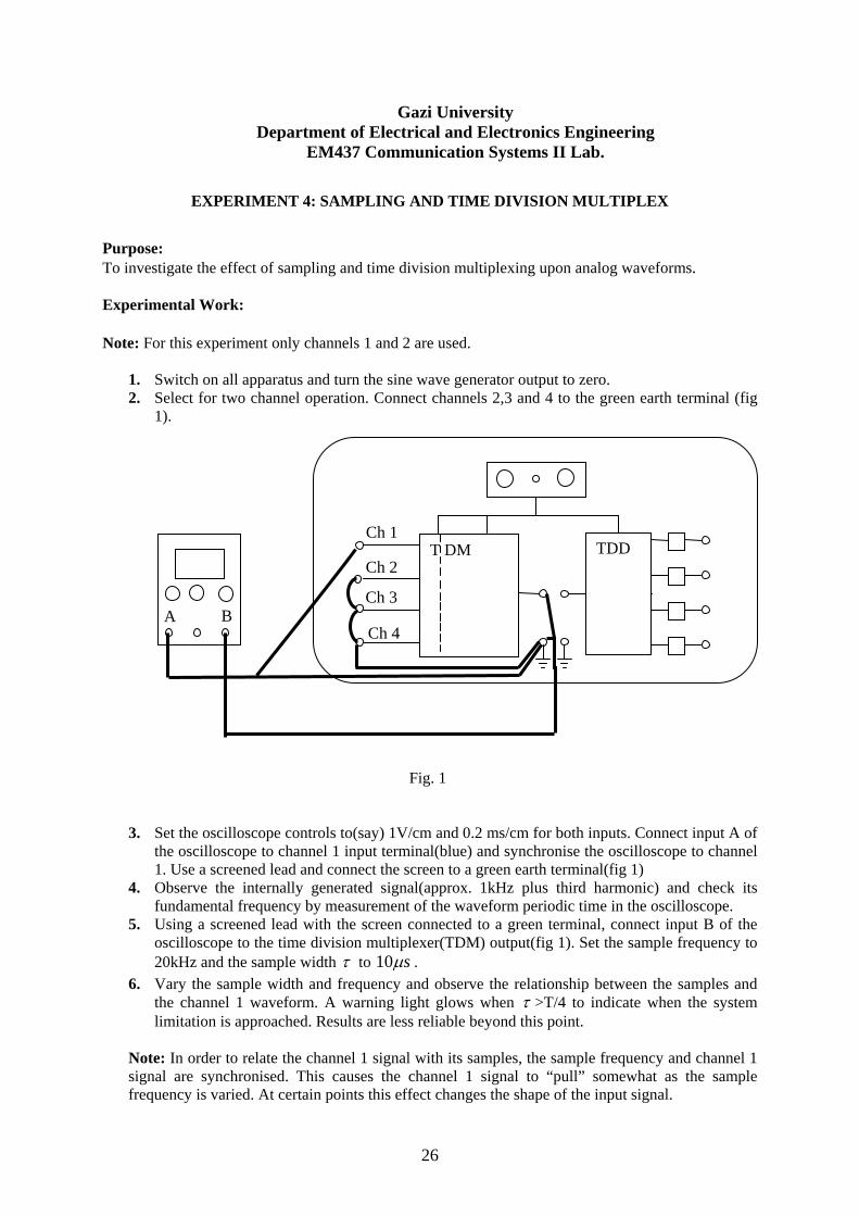
1. Switch on all apparatus and turn the sine wave generator output to zero. 2. Select for two channel operation. Connect channels 2,3 and 4 to the green earth terminal (fig

1).

Fig. 1

3. Set the oscilloscope controls to(say) 1V/cm and 0.2 ms/cm for both inputs. Connect input A of the oscilloscope to channel 1 input terminal(blue) and synchronise the oscilloscope to channel 1. Use a screened lead and connect the screen to a green earth terminal(fig 1)

4. Observe the internally generated signal(approx. 1kHz plus third harmonic) and check its fundamental frequency by measurement of the waveform periodic time in the oscilloscope.

5. Using a screened lead with the screen connected to a green terminal, connect input B of the oscilloscope to the time division multiplexer(TDM) output(fig 1). Set the sample frequency to 20kHz and the sample width τ to sμ10 .

6. Vary the sample width and frequency and observe the relationship between the samples and the channel 1 waveform. A warning light glows when τ >T/4 to indicate when the system limitation is approached. Results are less reliable beyond this point.

Note: In order to relate the channel 1 signal with its samples, the sample frequency and channel 1 signal are synchronised. This causes the channel 1 signal to “pull” somewhat as the sample frequency is varied. At certain points this effect changes the shape of the input signal.

T DM TDD

A B

Ch 1

Ch 2

Ch 3

Ch 4

27

7. Connect the TDM output to the time division demultiplexer(TDD) input. With input A of the

oscilloscope still connected to channel 1 input, connect input B of the oscilloscope to the TDD channel 1 output.

8. With a sample frequency of 20 kHz andτ = sμ10 , observe the channel 1 output waveform and compare it with the input waveform. Note any difference between the two waveforms.

9. Withτ kept at sμ10 , gradually reduce the sample frequency. Remembering the effect of synchronisation between channel 1 signal and the samples, note the input and output waveforms. Note also that the distortion at the output worsens as the sample frequency is reduced.

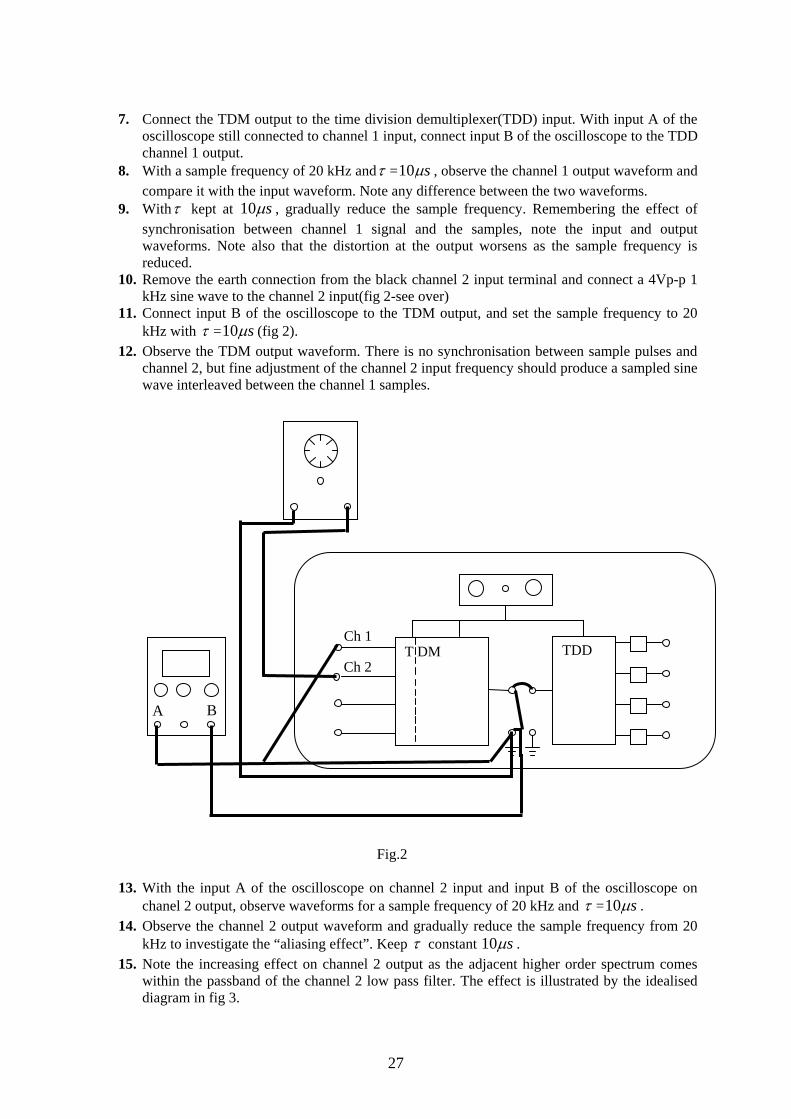
10. Remove the earth connection from the black channel 2 input terminal and connect a 4Vp-p 1 kHz sine wave to the channel 2 input(fig 2-see over)

11. Connect input B of the oscilloscope to the TDM output, and set the sample frequency to 20 kHz with τ = sμ10 (fig 2).

12. Observe the TDM output waveform. There is no synchronisation between sample pulses and channel 2, but fine adjustment of the channel 2 input frequency should produce a sampled sine wave interleaved between the channel 1 samples.

Fig.2

13. With the input A of the oscilloscope on channel 2 input and input B of the oscilloscope on chanel 2 output, observe waveforms for a sample frequency of 20 kHz and τ = sμ10 .

14. Observe the channel 2 output waveform and gradually reduce the sample frequency from 20 kHz to investigate the “aliasing effect”. Keep τ constant sμ10 .

15. Note the increasing effect on channel 2 output as the adjacent higher order spectrum comes within the passband of the channel 2 low pass filter. The effect is illustrated by the idealised diagram in fig 3.

T DM TDD

A B

Ch 1

Ch 2

28

16. The interference is a higher frequency sinusoidal wave and its amplitude is compared to the signal amplitude by the ratio a/s shown in fig 3. To make a measurement of a/s it is best to trigger the oscilloscope on channel A. It is not easy to measure the frequency of the interference but for an input frequency of f m and sampling frequency f s it is ( f s - f m ).

Fig. 3

17. With a sampling rate of 10 kHz and τ = sμ10 measure the ratio a/s. 18. Now gradually increase the width until τ is just less than T/4(indicated by the light and a

jump in the waveform). Measure a/s again noting that the value of a remains constant. Conclusion: Analogue signals can be sampled and then recovered provided the sampling frequency is at least twice the bandwidth of the signal and provided the output filter rejects the adjacent higher order spectrum. Sampled signals can be combined into one channel by time division multiplex and separated by demultiplexing. The width of the sampling pulses affects the spectrum of the sampled waveform. Wider pulses reduce the higher frequencies and hence reduce the aliasing noise. Equipment List: Dual beam oscilloscope, d.c. coupled, TecQuipment E15g. Audio frequency sine wave generator.